1st Meeting of the Scientific Committee of Western and Central Pacific Fisheries Commi

WCPFC–SC1 Noumea, New Caledonia 

8–19 August 2005 

Stock assessment of bigeye tunaO

John Hampton1, Pierre Kleiber2, AdIchin

1Oceanic Fisheries Programme, Secretariat of

2Pacific Islands Fishery Science Center, Natio3National Research Institute of

Augu

the ssion 

in the western and central Pacific cean

am Langley1, Yukio Takeuchi3 and Momoko okawa3

the Pacific Community, Noumea, New Caledonia

nal Marine Fisheries Service, Honolulu, Hawaii

Far Seas Fisheries, Shimizu, Japan

st 2005

SCTB17 Working Paper

SA–2

WCPFC–SC1 SA WP–2

i

Table of Contents Executive summary .............................................................................................................................. 1 1 Introduction ................................................................................................................................... 2 2 Background ................................................................................................................................... 2

2.1 Biology .................................................................................................................................. 2 2.2 Fisheries................................................................................................................................. 3

3 Data compilation ........................................................................................................................... 3 3.1 Spatial stratification............................................................................................................... 3 3.2 Temporal stratification .......................................................................................................... 4 3.3 Definition of fisheries............................................................................................................ 4 3.4 Catch and effort data ............................................................................................................. 4 3.5 Length-frequency data........................................................................................................... 4 3.6 Weight-frequency data .......................................................................................................... 5 3.7 Tagging data .......................................................................................................................... 5

4 Model description − structural assumptions, parameterisation, and priors ................................... 6 4.1 Population dynamics ............................................................................................................. 6

4.1.1 Recruitment...................................................................................................................... 6 4.1.2 Initial population .............................................................................................................. 7 4.1.3 Growth ............................................................................................................................. 7 4.1.4 Movement ........................................................................................................................ 7 4.1.5 Natural mortality .............................................................................................................. 7

4.2 Fishery dynamics................................................................................................................... 8 4.2.1 Selectivity......................................................................................................................... 8 4.2.2 Catchability ...................................................................................................................... 8 4.2.3 Effort deviations............................................................................................................... 8

4.3 Dynamics of tagged fish ........................................................................................................ 9 4.3.1 Tag mixing ....................................................................................................................... 9 4.3.2 Tag reporting.................................................................................................................... 9

4.4 Observation models for the data............................................................................................ 9 4.5 Parameter estimation ........................................................................................................... 10 4.6 Stock assessment interpretation methods ............................................................................ 10

4.6.1 Fishery impact................................................................................................................ 10 4.6.2 Yield analysis ................................................................................................................. 11

5 Sensitivity analyses ..................................................................................................................... 11 6 Results ......................................................................................................................................... 12

6.1 Fit statistics and convergence .............................................................................................. 12 6.2 Fit diagnostics (GLM-MFIX).............................................................................................. 12 6.3 Model parameter estimates.................................................................................................. 13

6.3.1 Growth ........................................................................................................................... 13

ii

6.3.2 Natural mortality ............................................................................................................ 13 6.3.3 Movement ...................................................................................................................... 13 6.3.4 Selectivity....................................................................................................................... 14 6.3.5 Catchability .................................................................................................................... 14 6.3.6 Tag-reporting rates ......................................................................................................... 14

6.4 Stock assessment results...................................................................................................... 14 6.4.1 Recruitment.................................................................................................................... 14 6.4.2 Biomass.......................................................................................................................... 15 6.4.3 Fishing mortality ............................................................................................................ 15 6.4.4 Fishery impact................................................................................................................ 15 6.4.5 Yield analysis ................................................................................................................. 15

7 Discussion and conclusions ......................................................................................................... 17 8 Acknowledgements ..................................................................................................................... 19 9 References ................................................................................................................................... 19 Appendix A: doitall.bet .....................................................................................................................A1 Appendix B: bet.ini ...........................................................................................................................B1

1

Executive summary This paper presents the 2005 assessment of bigeye tuna in the western and central Pacific

Ocean. The assessment uses the stock assessment model and computer software known as MULTIFAN-CL. The bigeye tuna model is age (40 age-classes) and spatially structured (6 regions) and the catch, effort, size composition and tagging data used in the model are classified by 20 fisheries and quarterly time periods from 1952 through 2004.

Six independent analyses are conducted to test the impact of using different methods of standardising fishing effort in the main longline fisheries, using estimated or assumed values of natural mortality-at-age, and assuming certain arbitrary increases in fishing power for the main longline and purse seine fleets. The analyses conducted are:

SHBS-MEST Statistical habitat-based standardised effort for main longline fisheries, M (assumed constant across age-class) estimated.

SHBS-MFIX Statistical habitat-based standardised effort for main longline fisheries, M-at-age assumed at fixed levels.

GLM-MEST General linear model standardised effort for main longline fisheries, M (assumed constant across age-class) estimated.

GLM-MFIX General linear model standardised effort for main longline fisheries, M-at-age assumed at fixed levels.

FPOW-MEST General linear model standardised effort for main longline fisheries, M (assumed constant across age-class) estimated. Fishing power expansions incorporated into longline (1% per year) and purse seine (4 % per year) effort. No other temporal trends in catchability for these fisheries.

FPOW-MFIX General linear model standardised effort for main longline fisheries, M-at-age assumed at fixed levels. Fishing power expansions incorporated into longline (1% per year) and purse seine (4 % per year) effort. No other temporal trends in catchability for these fisheries.

The order (from best to worst) of the models in terms of their fit to the composite data and prior assumptions was: FPOW-MEST, GLM-MEST, FPOW-MFIX, GLM-MFIX, SHBS-MEST and SHBS-MFIX.

The catch, size and tagging data used in the assessment were the same as those used last year, with the exception that additional recent fishery data (2003 and 2004 for longline, 2003 for Philippines and Indonesia, 2004 for purse seine) was included. It should be noted that 2004 data are not complete for some fisheries. The estimation of standardised effort for the main longline fisheries using the GLM and SHBS approaches involved a new method of scaling indices of abundance among regions (see Langley et al. 2005 for details). Overall, the new procedure resulted in higher relative abundance in the tropical regions (3 and 4) and lower relative abundance in the northern (1 and 2) and southern (5 and 6) regions compared to the method used in previous years.

The SHBS- and GLM-based analyses produced results that were broadly comparable to those of recent assessments. Recruitment showed an increasing trend from the 1970s on, while biomass declined through the 1960s and 1970s after which it was relatively stable or declining slightly. The fisheries are estimated to have reduced overall biomass to 30-50% of unfished levels by 2004, with impacts more severe in the equatorial region of the WCPO, particularly in the west. Yield analyses suggest that recent average fishing mortality-at-age is near to or above the fishing mortality at Maximum Sustainable Yield (MSY). On the other hand, the current level of total biomass is estimated to be above equilibrium biomass expected at MSY, with the exception of those analyses assuming fishing power increases in the main longline and purse seine fisheries. In the latter analyses, total biomass is marginally above the MSY level and the current adult biomass is below the MSY level.

2

Current biomass is generally above equilibrium levels because of above-average recruitment since about 1990.

On the basis of all of the results presented in the assessment, we conclude that maintenance of current levels of fishing mortality carries a high risk of overfishing. Should recruitment fall to average levels, current fishing mortality would result in stock reductions to near and possibly below MSY-based reference points.

1 Introduction This paper presents the current stock assessment of bigeye tuna (Thunnus obesus) in the

western and central Pacific Ocean (WCPO, west of 150°W). A comparison of results with those from a similarly-structured Pacific-wide analysis is given in a separate paper (Hampton and Maunder 2005). The overall objectives of the assessment are to estimate population parameters, such as time series of recruitment, biomass and fishing mortality, that indicate the status of the stock and impacts of fishing. We summarise stock status in terms of well-known reference points, such as the ratios of recent stock biomass to the biomass at maximum sustainable yield ( MSYcurrent BB ~ ) and recent fishing mortality to the fishing mortality at MSY ( MSYcurrent FF ~ ). Likelihood profiles of these ratios are used to describe their uncertainty.

The underlying methodology used for the assessment is that commonly known as MULTIFAN-CL (Fournier et al. 1998; Hampton and Fournier 2001; Kleiber et al. 2003; http://www.multifan-cl.org), which is software that implements a size-based, age- and spatially-structured population model. Parameters of the model are estimated by maximizing an objective function consisting of likelihood (data) and prior information components.

2 Background

2.1 Biology Bigeye tuna are distributed throughout the tropical and sub-tropical waters of the Pacific

Ocean. There is little information on the extent of mixing across this wide area. Analysis of mtDNA and DNA microsatellites in nearly 800 bigeye tuna failed to reveal significant evidence of widespread population subdivision in the Pacific Ocean (Grewe and Hampton 1998). While these results are not conclusive regarding the rate of mixing of bigeye tuna throughout the Pacific, they are broadly consistent with the results of SPC’s tagging experiments on bigeye tuna. Bigeye tuna tagged in locations throughout the western tropical Pacific have displayed movements of up to 4,000 nautical miles (Figure 1) over periods of one to several years, indicating the potential for gene flow over a wide area; however, the large majority of tag returns were recaptured much closer to their release points. Also, recent tagging experiments in the eastern Pacific Ocean (EPO) using archival tags have so far not demonstrated long-distance migratory behaviour (Schaefer and Fuller 2002) over relatively short time scales (up to 3 years). In view of these results, stock assessments of bigeye tuna are routinely undertaken for the WCPO and EPO separately1.

Bigeye tuna are relatively fast growing, and have a maximum fork length (FL) of about 200 cm. The growth of juveniles departs from von Bertalanffy type growth with the growth rate slowing between about 40 and 70 cm FL (Lehodey et al. 1999). The natural mortality rate is likely to be variable with size, with the lower rates of around 0.5 yr-1 for bigeye >40 cm FL (Hampton 2000). Tag recapture data indicate that significant numbers of bigeye reach at least eight years of age. The longest

1 Efforts continue to develop a bigeye tuna model for the Pacific Ocean as a whole, incorporating spatial structure into the analysis to allow for the possibility of restricted movement between some areas. The results of the most recent Pacific-wide model are compared with the WCPO results and the results of the most recent IATTC assessment for the EPO in Hampton and Maunder (2005).

3

period at liberty for a recaptured bigeye tuna tagged in the western Pacific at about 1−2 years of age is currently 12 years (Hampton and Williams 2004).

2.2 Fisheries Bigeye tuna are an important component of tuna fisheries throughout the Pacific Ocean and

are taken by both surface gears, mostly as juveniles, and longline gear, as valuable adult fish. They are a principal target species of both the large, distant-water longliners from Japan and Korea and the smaller, fresh sashimi longliners based in several Pacific Island countries. Prices paid for both frozen and fresh product on the Japanese sashimi market are the highest of all the tropical tunas. Bigeye tuna are the cornerstone of the tropical longline fishery in the WCPO; the catch in the SPC area had a landed value in 2001 of approximately US$1 billion.

Since 1980, the longline catch of bigeye tuna in the WCPO has varied between about 40,000 and 60,000 t (Figure 2), with the record high catch being taken in 2002. Since about 1994, there has been a rapid increase in purse-seine catches of juvenile bigeye tuna, first in the eastern Pacific Ocean (EPO) and since 1996, to a lesser extent, in the WCPO. In the WCPO, purse-seine catches of bigeye tuna are estimated to have been less than 20,000 t per year up to 1996, mostly from sets on natural floating objects (Hampton et al. 1998). In 1997, the catch increased to 35,000 t, primarily as a result of increased use of fish aggregation devices (FADs). High purse seine catches were also recorded in 1999 (38,000 t) and 2000 (33,000 t).

The spatial distribution of WCPO bigeye tuna catch during 1990−2004 is shown in Figure 3. The majority of the catch is taken in equatorial areas, by both purse seine and longline, but with significant longline catch in some sub-tropical areas (east of Japan, north of Hawaii and the east coast of Australia). High catches are also presumed to be taken in the domestic artisanal fisheries of Philippines and Indonesia. These catches, along with small catches by pole-and-line vessels operating in various parts of the WCPO, have approached 20,000 t in recent years. The statistical basis for the catch estimates in Philippines and Indonesia is weak; however, we have included the best available estimates in this analysis in the interests of providing the best possible coverage of bigeye tuna catches in the WCPO.

3 Data compilation The data used in the bigeye tuna assessment consist of catch, effort, length-frequency and

weight-frequency data for the fisheries defined in the analysis, and tag release-recapture data. The details of these data and their stratification are described below.

3.1 Spatial stratification The geographic area considered in the assessment is the WCPO, defined by the coordinates

40°N−35°S, 120°E−150°W. Within this overall area, a six-region spatial stratification was adopted for the assessment (Figure 3). The rationale for this stratification was to separate the tropical area, where both surface and longline fisheries occur year-round, from the higher latitudes, where the longline fisheries occur more seasonally. The stratification is different to that used in the 2004 assessment, in response to discussions held at SCTB 17 and subsequently. The area north of 20°N has been split into two regions, while the boundary separating eastern and western regions has been shifted from 160°E to 170°E. Time series of total catches by major gear categories are shown in Figure 4. Most of the catch occurs in the tropical regions (3 and 4), with most juvenile catches (by purse seine and Philippines/Indonesian fisheries) occurring in region 3 and large longline catches occurring in both regions 3 and 4.

4

3.2 Temporal stratification The primary time period covered by the assessment is 1952−2004, thus including all

significant post-war tuna fishing in the WCPO. Within this period, data were compiled into quarters (Jan−Mar, Apr−Jun, Jul−Sep, Oct−Dec).

3.3 Definition of fisheries MULTIFAN-CL requires the definition of “fisheries” that consist of relatively homogeneous

fishing units. Ideally, the fisheries so defined will have selectivity and catchability characteristics that do not vary greatly over time (although in the case of catchability, some allowance can be made for time-series variation). Twenty fisheries have been defined for this analysis on the basis of region, gear type and, in the case of purse seine, set type (Table 1).

3.4 Catch and effort data Catch and effort data were compiled according to the fisheries defined above. Catches by the

longline fisheries were expressed in numbers of fish, and catches for all other fisheries expressed in weight. This is consistent with the form in which the catch data are recorded for these fisheries. Purse seine catches of bigeye are not reliably recorded on logsheets for most fleets, and must be estimated from sampling data. The method used to derive such estimates for the purse seine fishery is based on the two-variable (set type and year) analysis of variance described in Lawson (2005).

Effort data for the Philippines and Indonesian fisheries were unavailable and the relative catch was used as a proxy for effort. Alternatively, we could have defined effort for these fisheries to be missing, in which case the relative effort over time would have been determined only by the effort deviations, which have a lognormal probability distribution with constant mean and variance. We felt that it was better to have a “null hypothesis” of effort proportional to catch, rather than constant over time. In practice, this assumption has not been found to influence the results overly, as the variance of the catchability deviations for these fisheries is set at a high level to give the model flexibility to fit the total catch. This approach also facilitated effort-based projections (Hampton et al. 2005).

Effort data units for purse seine fisheries are defined as days fishing and/or searching, allocated to set types based on the proportion of total sets attributed to a specified set type (log, FAD or school sets) in logbook data. For the longline fisheries, we used two estimates of effective (or standardised) effort derived in a separate study (Langley et al. 2005). Separate analyses were undertaken for both longline effort series. The effort series used were those estimated using a general linear model (GLM) and an unconstrained statistical habitat-based standardisation (SHBS). Time-series of catch and catch-per-unit-effort (CPUE) for all fisheries, and CPUE constructed using the two sets of longline effort data are shown in Figure 5, Figure 6 and Figure 7, respectively.

Within the model, effort for each fishery was normalised to an average of 1.0 to assist numerical stability. Some longline fisheries were grouped to share common catchability parameters in the various analyses. For such grouped fisheries, the normalisation occurred over the group rather than for the individual fisheries so as to preserve the relative levels of effort between the fisheries. In the standardisation of longline effort, the scaling of standardised CPUE among regions included a correction to allow for the effective area exploited by the fishery in each region. Therefore longline standardised CPUE can be interpreted as an index of exploitable abundance in each region (rather than density).

3.5 Length-frequency data Available length-frequency data for each of the defined fisheries were compiled into 95 2-cm

size classes (10−12 cm to 188−200 cm). Each length-frequency observation consisted of the actual number of bigeye tuna measured. A graphical representation of the availability of length (and weight) samples is provided in Figure 8. The data were collected from a variety of sampling programmes, which can be summarized as follows:

5

Philippines: Size composition data for the Philippines domestic fisheries derived from a sampling programme conducted in the Philippines in 1993−94 were augmented with data from the 1980s and for 1995. In addition, data collected during 1997−2002 from the Philippines hand-line (PH HL 3) and surface fisheries (PHID MISC 3) under the National Stock Assessment Project (NSAP) were included in the current assessment.

Indonesia: Limited size data were obtained for the Indonesian domestic fisheries from the former IPTP database. Note that the miscellaneous Indonesian fishery has been combined with the Philippines small-fish fishery in this assessment, and therefore the size composition of the catch is assumed to be represented by the combined data.

Purse seine: Length-frequency samples from purse seiners have been collected from a variety of port sampling and observer programmes since the mid-1980s. Most of the early data is sourced from the U.S. National Marine Fisheries Service (NMFS) port sampling programme for U.S. purse seiners in Pago Pago, American Samoa and an observer programme conducted for the same fleet. Since the early 1990s, port sampling and observer programmes on other purse seine fleets have provided additional data. Only data that could be classified by set type were included in the final data set. For each purse seine fishery, size samples were aggregated without weighting within temporal strata.

Longline: The majority of the historical data were collected by port sampling programmes for Japanese longliners unloading in Japan and from sampling aboard Japanese research and training vessels. It is assumed that these data are representative of the sizes of longline-caught bigeye in the various model regions. Japanese data for 1952−1964 have recently become available, and are included in the assessment. In recent years, data have also been collected by OFP and national port sampling and observer programmes in the WCPO.

3.6 Weight-frequency data Individual weight data for the Japanese longline fisheries are included in this assessment in

their original form. For many other longline fleets, “packing list” data are available from export documentation, and these data are progressively being processed and incorporated into the assessment database. For this assessment, the available weight data (apart from those provided by Japan) originated from vessels unloading in various ports around the region from where tuna are exported, including Guam, Palau, FSM, Marshall Islands, Fiji, Papua New Guinea and eastern Australian ports. Data were compiled by 1 kg weight intervals over a range of 1−150 kg. As the weights were generally gilled-and-gutted weights, the frequency intervals were adjusted by a gilled-and-gutted to whole weight conversion factor for bigeye tuna (1.1018). The time-series distribution of available weight samples is shown in Figure 8.

3.7 Tagging data A modest amount of tagging data was available for incorporation into the MULTIFAN-CL

analysis. The data used consisted of bigeye tuna tag releases and returns from the OFP’s Regional Tuna Tagging Project conducted during 1989−1992, and more recent releases and returns from tagging conducted in the Coral Sea by CSIRO. We considered including a large number of tags released in the Hawaii handline fishery in recent years; however inclusion of these data caused large changes in movement estimates between regions 2 and 4 and other parameters because these tags were released close to the region boundary. We therefore opted not to include these data in the current assessment until these effects could be more fully evaluated.

Tags were released using standard tuna tagging equipment and techniques by trained scientists and technicians. The tag release effort was spread throughout the tropical western Pacific, between approximately 120°E and 170°W (Kaltongga 1998; Hampton and Williams 2004).

For incorporation into the MULTIFAN-CL analyses, tag releases were stratified by release region (all bigeye tuna releases occurred in regions 3, 4 and 5), time period of release (quarter) and the same length classes used to stratify the length-frequency data. A total of 14,045 releases were

6

classified into 23 tag release groups in this way. 962 tag returns were received that could be assigned to the fisheries included in the model. Tag returns that could not be so assigned were included in the non-reported category and appropriate adjustments made to the tag-reporting rate priors and bounds. The returns from each size class of each tag release group were then classified by recapture fishery and recapture time period (quarter). Because tag returns by purse seiners were often not accompanied by information concerning the set type, tag-return data were aggregated across set types for the purse seine fisheries in each region. The population dynamics model was in turn configured to predict equivalent estimated tag recaptures by these grouped fisheries.

4 Model description − structural assumptions, parameterisation, and priors

The model can be considered to consist of several components, (i) the dynamics of the fish population; (ii) the fishery dynamics; (iii) the dynamics of tagged fish; (iv) observation models for the data; (v) parameter estimation procedure; and (vi) stock assessment interpretations. Detailed technical descriptions of components (i) − (iv) are given in Hampton and Fournier (2001) and are not repeated here. Rather, brief descriptions of the various processes are given, including information on structural assumptions, estimated parameters, priors and other types of penalties used to constrain the parameterisation. For convenience, these descriptions are summarized in Table 2. In addition, we describe the procedures followed for estimating the parameters of the model and the way in which stock assessment conclusions are drawn using a series of reference points.

4.1 Population dynamics The model partitions the population into 6 spatial regions and 40 quarterly age-classes. The

first age-class has a mean fork length of around 25 cm and is approximately three months of age according to analysis of daily structures on otoliths (Lehodey et al. 1999). The last age-class comprises a “plus group” in which mortality and other characteristics are assumed to be constant. For the purpose of computing the spawning biomass, we assume that the proportions mature in each age- class are as follows:

Age-class 1-10 11 12 13 14 15 16 17 18 19 20 21−40

Proportion mature 0.0 0.05 0.10 0.20 0.40 0.60 0.70 0.80 0.85 0.90 0.95 1.00

The population is “monitored” in the model at quarterly time steps, extending through a time window of 1952−2004. The main population dynamics processes are as follows:

4.1.1 Recruitment

Recruitment is the appearance of age-class 1 fish in the population. We have assumed that recruitment occurs instantaneously at the beginning of each quarter. This is a discrete approximation to continuous recruitment, but provides sufficient flexibility to allow a range of variability to be incorporated into the estimates as appropriate.

The distribution of recruitment among the six model regions was estimated within the model and allowed to vary over time in a relatively unconstrained fashion. The time-series variation in spatially-aggregated recruitment was somewhat constrained by a lognormal prior. The variance of the prior was set such that recruitments of about three times and one third of the average recruitment would occur about once every 25 years on average.

Spatially-aggregated recruitment was assumed to have a weak relationship with the parental biomass via a Beverton and Holt stock-recruitment relationship (SRR). The SRR was incorporated mainly so that a yield analysis could be undertaken for stock assessment purposes. We therefore opted to apply a relatively weak penalty for deviation from the SRR so that it would have only a slight effect on the recruitment and other model estimates (see Hampton and Fournier 2001, Appendix D).

7

Typically, fisheries data are not very informative about SRR parameters and it is generally necessary to constrain the parameterisation in order to have stable model behaviour. We incorporated a beta-distributed prior on the “steepness” (S) of the SRR, with S defined as the ratio of the equilibrium recruitment produced by 20% of the equilibrium unexploited spawning biomass to that produced by the equilibrium unexploited spawning biomass (Francis 1992; Maunder and Watters 2003). The prior was specified by mode = 0.85 and SD = 0.16 (a = 3.1, b = 1.6, lower bound = 0.2, upper bound = 1.0). This is a somewhat weaker prior than has been used in the past, but we feel that it better reflects our knowledge of tuna stock-recruitment relationships. The prior probability distribution for steepness is shown in Figure 9.

4.1.2 Initial population

The population age structure in the initial time period in each region was assumed to be in equilibrium and determined as a function of the average total mortality during the first 20 quarters. This assumption avoids having to treat the initial age structure, which is generally poorly determined, as independent parameters in the model. Note that the assumption used does not assume virgin conditions at the start of the assessment data. Rather, we assume that exploitation in the years leading up to 1952 was similar to exploitation over the period 1952−1956. This probably overestimates total mortality in the initial population, but the bias should be minimal. The initial age structure was applied to the initial recruitment estimates to obtain the initial populations in each region.

4.1.3 Growth

The standard assumptions made concerning age and growth are (i) the lengths-at-age are normally distributed for each age-class; (ii) the mean lengths-at-age follow a von Bertalanffy growth curve; (iii) the standard deviations of length for each age-class are a log-linear function of the mean lengths-at-age; and (iv) the distribution of weight-at-age is a deterministic function of the length-at-age and a specified weight-length relationship (see Table 2). As noted above, the population is partitioned into 40 quarterly age-classes.

Previous analyses assuming a standard von Bertalanffy growth pattern indicated that there was substantial departure from the model, particularly for sizes up to about 80 cm. Similar observations have been made on bigeye tuna growth patterns determined from daily otolith increments and tagging data (Lehodey et al. 1999). We therefore modelled growth by allowing the mean lengths of the first eight quarterly age-classes to be independent parameters, with the remaining mean lengths following a von Bertalanffy growth curve. These deviations attract a small penalty to avoid over-fitting the size data.

4.1.4 Movement

Movement was assumed to occur instantaneously at the beginning of each quarter through movement coefficients connecting regions sharing a common boundary. Note however that fish can move between non-contiguous regions in a single time step due to the “implicit transition” computational algorithm employed (see Hampton and Fournier 2001 for details). There are seven inter-regional boundaries in the model with movement possible across each in both directions. Four seasonal movements were allowed, each with their own movement coefficients. Thus there is a need for 2×7×4 = 56 movement parameters. We did not incorporate age-dependent movement into this assessment, to avoid the addition of more parameters. Trials indicated that this additional structure did not impact the overall results in a substantive way. The seasonal pattern of movement persists from year to year with no allowance for longer-term variation in movement.

4.1.5 Natural mortality

Natural mortality (M) was either held fixed at pre-determined age-specific levels (MFIX) or was estimated as a single parameter with no age-related variability (MEST). We did not estimate M-at-age in these assessments because trial fits estimating M-at-age produced biologically unreasonable results. For the fixed M runs, M-at-age was determined outside of the MULTIFAN-CL model using bigeye sex-ratio data and the assumed maturity-at-age schedule. An identical procedure is used to determine fixed M-at-age for assessments in the EPO (Maunder 2005). Essentially, this method

8

reflects the hypothesis that the higher proportion of males in sex-ratio samples with increasing length is due to the higher natural mortality of females after they reach maturity. The externally-estimated M-at-age used for the MFIX runs is shown in Figure 10.

4.2 Fishery dynamics The interaction of the fisheries with the population occurs through fishing mortality. Fishing

mortality is assumed to be a composite of several separable processes − selectivity, which describes the age-specific pattern of fishing mortality; catchability, which scales fishing effort to fishing mortality; and effort deviations, which are a random effect in the fishing effort − fishing mortality relationship.

4.2.1 Selectivity

In many stock assessment models, selectivity is modelled as a functional relationship with age, e.g. using a logistic curve to model monotonically increasing selectivity and various dome-shaped curves to model fisheries that select neither the youngest nor oldest fish. In previous assessments, we have modelled selectivity with separate age-specific coefficients (with a range of 0−1), but constraining the parameterisation with smoothing penalties. This has the disadvantage of requiring a large number of parameters to describe selectivity. In this assessment we have used a new method based on a cubic spline interpolation to estimate age-specific selectivity. This is a form of smoothing, but the number of parameters for each fishery is the number of cubic spline “nodes” that are deemed to be sufficient to characterise selectivity over the age range. We chose five nodes, which seems to be sufficient to allow for reasonably complex selectivity patterns.

Selectivity is assumed to be fishery-specific and time-invariant. For the longline fisheries (which catch mainly adult bigeye) selectivity was assumed to increase with age and to remain at the maximum once attained. Selectivity coefficients for the “main” longline fisheries LL ALL 1 and LL ALL 2 (northern fisheries) were constrained to be equal, as were LL ALL 3-6 (equatorial and southern fisheries). The coefficients for the last four age-classes, for which the mean lengths are very similar, were constrained to be equal for all fisheries.

4.2.2 Catchability

Catchability was allowed to vary slowly over time (akin to a random walk) for all purse seine fisheries, the Philippines and Indonesian fisheries, the Australian, Taiwanese/Chinese, Hawaii, PNG and other Pacific-Island longline fisheries, using a structural time-series approach. Random walk steps were taken every two years, and the deviations were constrained by prior distributions of mean zero and variance specified for the different fisheries according to our prior belief regarding the extent to which catchability may have changed. For the Philippines and Indonesian fisheries, no effort estimates were available. We made the prior assumption that effort for these fisheries was proportional to catch, but set the variance of the priors to be high (approximating a CV of about 0.7), thus allowing catchability changes to compensate for failure of this assumption. For the other fisheries with time-series variability in catchability, the catchability deviation priors were assigned a variance approximating a CV of 0.10.

The “main” longline fisheries were grouped for the purpose of initial catchability, and time-series variation was assumed not to occur in this group. This assumption is equivalent to assuming that the CPUE for these fisheries indexes the exploitable abundance both among areas and over time.

Catchability for all fisheries apart from the Philippines and Indonesian fisheries (in which the data were based on annual estimates) was allowed to vary seasonally.

4.2.3 Effort deviations

Effort deviations, constrained by prior distributions of zero mean, were used to model the random variation in the effort – fishing mortality relationship. For the Philippines and Indonesian fisheries, for which reliable effort data were unavailable, we set the prior variance at a high level (approximating a CV of 0.7), to allow the effort deviations to account for short-term fluctuations in

9

the catch caused by variation in real effort. For the purse seine fisheries and the Australian, Hawaii and Taiwanese-Chinese longline fisheries, the variance was set at a moderate level (approximating a CV of 0.2). For the main longline fisheries (LL ALL 1-6), the variance was set at a lower level (approximating a CV of 0.1) because the effort had been standardised in prior analyses and these longline fisheries provide wide spatial coverage of the respective areas in which they occur.

4.3 Dynamics of tagged fish 4.3.1 Tag mixing

In general, the population dynamics of the tagged and untagged populations are governed by the same model structures and parameters. An obvious exception to this is recruitment, which for the tagged population is simply the release of tagged fish. Implicitly, we assume that the probability of recapturing a given tagged fish is the same as the probability of catching any given untagged fish in the same region. For this assumption to be valid, either the distribution of fishing effort must be random with respect to tagged and untagged fish and/or the tagged fish must be randomly mixed with the untagged fish. The former condition is unlikely to be met because fishing effort is almost never randomly distributed in space. The second condition is also unlikely to be met soon after release because of insufficient time for mixing to take place. Depending on the disposition of fishing effort in relation to tag release sites, the probability of capture of tagged fish soon after release may be different to that for the untagged fish. It is therefore desirable to designate one or more time periods after release as “pre-mixed” and compute fishing mortality for the tagged fish based on the actual recaptures, corrected for tag reporting (see below), rather than use fishing mortalities based on the general population parameters. This in effect desensitises the likelihood function to tag recaptures in the pre-mixed periods while correctly discounting the tagged population for the recaptures that occurred.

We assumed that tagged bigeye mix fairly quickly with the untagged population at the region level and that this mixing process is complete by the end of the second quarter after release.

4.3.2 Tag reporting

In principal, tag-reporting rates can be estimated internally within the model. In practice, experience has shown that independent information on tag reporting rates for at least some fisheries tends to be required for reasonably precise estimates to be obtained. We provided reporting rate priors for all fisheries that reflect our prior opinion regarding the reporting rate and the confidence we have in that opinion. Relatively informative priors were provided for reporting rates for the Philippines and Indonesian domestic fisheries and the purse seine fisheries, as independent estimates of reporting rates for these fisheries were available from tag seeding experiments and other information (Hampton 1997). For the longline fisheries, we have no auxiliary information with which to estimate reporting rates, so relatively uninformative priors were used for those fisheries. All reporting rates were assumed to be stable over time. The proportions of tag returns rejected from the analysis because of insufficient data were incorporated into the reporting rate priors.

4.4 Observation models for the data There are four data components that contribute to the log-likelihood function − the total catch

data, the length-frequency data, the weight-frequency data and the tagging data. The observed total catch data are assumed to be unbiased and relatively precise, with the SD of residuals on the log scale being 0.07.

The probability distributions for the length-frequency proportions are assumed to be approximated by robust normal distributions, with the variance determined by the effective sample size and the observed length-frequency proportion. Effective sample size is assumed to be 0.1 times the actual sample size, with a maximum effective sample size of 100. Reduction of the effective sample size recognises that (i) length-frequency samples are not truly random (because of clumping in the population with respect to size) and would have higher variance as a result; and (ii) the model

10

does not include all possible process error, resulting in further under-estimation of variances. A similar likelihood function was used for the weight-frequency data.

A log-likelihood component for the tag data was computed using a negative binomial distribution in which fishery-specific variance parameters were estimated from the data. The negative binomial is preferred over the more commonly used Poisson distribution because tagging data often exhibit more variability than can be attributed by the Poisson. We have employed a parameterisation of the variance parameters such that as they approach infinity, the negative binomial approaches the Poisson. Therefore, if the tag return data show high variability (for example, due to contagion or non-independence of tags), then the negative binomial is able to recognise this. This should then provide a more realistic weighting of the tag return data in the overall log-likelihood and allow the variability to impact the confidence intervals of estimated parameters. A complete derivation and description of the negative binomial likelihood function for tagging data is provided in Hampton and Fournier (2001) (Appendix C).

4.5 Parameter estimation The parameters of the model were estimated by maximizing the log-likelihoods of the data

plus the log of the probability density functions of the priors and smoothing penalties specified in the model. The maximization was performed by an efficient optimization using exact derivatives with respect to the model parameters. Estimation was conducted in a series of phases, the first of which used arbitrary starting values for most parameters. A bash script documenting the phased procedure is provided in Appendix A. Some parameters were assigned specified starting values consistent with available biological information. The values of these parameters are provided in the ini file (Appendix B). Details of the structure of these and other files used by MULTIFAN-CL are provided in the User’s Guide (Kleiber et al. 2003).

The Hessian matrix computed at the mode of the posterior distribution was used to obtain estimates of the covariance matrix, which was used in combination with the Delta method to compute approximate confidence intervals for parameters of interest. In addition, the likelihood profile method was used to generate probability distributions for the critical reference points MSYcurrent FF ~

and

MSYcurrent BB ~ . Likelihood profiles were generated by undertaking model runs with either

MSYcurrent FF ~ or MSYcurrent BB ~ set at various levels (by applying a penalty to the likelihood function for deviations from the target ratio) over the range of possible values. The likelihood function values resulting from these runs were then used to construct a probability distribution for each ratio.

4.6 Stock assessment interpretation methods Several ancillary analyses are conducted in order to interpret the results of the model for stock

assessment purposes. The methods involved are summarized below and the details can be found in Kleiber et al. (2003). Note that, in each case, these ancillary analyses are completely integrated into the model, and therefore confidence intervals for quantities of interest are available using the Hessian-Delta approach (or likelihood profile approach in the case of yield analysis results).

4.6.1 Fishery impact

Many assessments estimate the ratio of recent to initial biomass as an index of fishery depletion. The problem with this approach is that recruitment may vary considerably throughout the time series, and if either the initial or recent biomass estimates (or both) are “non-representative” because of recruitment variability, then the ratio may not measure fishery depletion, but simply reflect recruitment variability.

We approach this problem by computing biomass time series (at the region level) using the estimated model parameters, but assuming that fishing mortality was zero. Because both the real biomass Bt and the unexploited biomass B0t incorporate recruitment variability, their ratio at each time

11

step of the analysis t

t

BB

0 can be interpreted as an index of fishery depletion. The computation of

unexploited biomass includes an adjustment in recruitment to acknowledge the possibility of reduction of recruitment in exploited populations through stock-recruitment effects.

4.6.2 Yield analysis

The yield analysis consists of computing equilibrium catch (or yield) and biomass, conditional on a specified basal level of age-specific fishing mortality (Fa) for the entire model domain, a series of fishing mortality multipliers, fmult, the natural mortality-at-age (Ma), the mean weight-at-age (wa) and the SRR parameters α and β. All of these parameters, apart from fmult, which is arbitrarily specified over a range of 0−50 in increments of 0.1, are available from the parameter estimates of the model. The maximum yield with respect to fmult can easily be determined and is equivalent to the MSY. Similarly the total and adult biomass at MSY can also be determined. The ratios of the current (or recent average) levels of fishing mortality and biomass to their respective levels at MSY are of interest as limit reference points. These ratios are also determined and their confidence intervals estimated using a likelihood profile technique, as noted above.

For the standard yield analysis, the Fa are determined as the average over some recent period of time. In this assessment, we use the average over the period 2001−2003. The last year in which catch and effort data are available for all fisheries is 2004. We do not include 2004 and subsequent years in the average as fishing mortality tends to have high uncertainty for the terminal data years of the analysis and the catch and effort data for this terminal year are incomplete for some fisheries.

The assessments indicate that recruitment over the last two decades was higher than for the preceding period. Consequently, yield estimates based on the long-term equilibrium recruitment estimated from a Beverton and Holt SRR may substantially under-estimate the yields currently available from the stock under current recruitment conditions. For this reason, a separate yield analysis was conducted based on the average level of recruitment from 1994−2003.

5 Sensitivity analyses Standardised effort for the “main” longline fisheries (LL ALL 1−6) was estimated using two

alternative standardisation methods: one based on a GLM and the other on a statistical habitat-based standardisation (Langley et al. 2005). We also conducted a series of runs in which the effort data for longline and purse seine fisheries were expanded by 1% and 4%, respectively, per year from the base year to mimic expansion of fishing power.

Sensitivity to natural mortality estimates was investigated by conducting separate runs in which M-at-age was fixed and runs in which a generic M assumed constant across age-class was estimated. The fixed M-at-age used in these runs is shown in Figure 10..

In summary, the analyses carried out are:

SHBS-MEST Statistical habitat-based standardised effort for “main” longline fisheries, M (assumed constant across age-class) estimated.

SHBS-MFIX Statistical habitat-based standardised effort for “main” longline fisheries, M-at-age assumed at fixed levels.

GLM-MEST General linear model standardised effort for “main” longline fisheries, M (assumed constant across age-class) estimated.

GLM-MFIX General linear model standardised effort for “main” longline fisheries, M-at-age assumed at fixed levels.

FPOW-MEST General linear model standardised effort for “main” longline fisheries, M (assumed constant across age-class) estimated. Fishing power expansions

12

incorporated into longline (1% per year) and purse seine (4 % per year) effort. No other temporal trends in catchability for these fisheries.

FPOW-MFIX General linear model standardised effort for “main” longline fisheries, M-at-age assumed at fixed levels. Fishing power expansions incorporated into longline (1% per year) and purse seine (4 % per year) effort. No other temporal trends in catchability for these fisheries.

6 Results Results for the five analyses are presented below. In the interests of brevity, some categories

of results are presented for the GLM-MFIX analysis only, which is designated the base-case analysis. However, the main stock assessment-related results are summarised for all analyses.

6.1 Fit statistics and convergence A summary of the fit statistics for the six analyses is given in Table 3 from which the

following observations can be made:

o The GLM-based analyses provide much better fits to the data and prior assumptions than the SHBS-based analyses. The main source of improvement was in the fits to the total catches and a lower penalty component for the effort deviations. This indicates that the GLM-based longline effort was more consistent with the observed catches than the SHBS effort.

o The FPOW analyses, which incorporated fishing power assumptions to adjust GLM-based longline effort and purse seine effort, provided even better overall fits to the data and prior assumptions.

o The MEST fits were superior to the MFIX fits for each analysis category.

o The order (from best to worst) of the models in terms of their fit to the composite data and prior assumptions was: FPOW-MEST, GLM-MEST, FPOW-MFIX, GLM-MFIX, SHBS-MEST and SHBS-MFIX.

In order to verify (to the extent possible) that our final fit to the data was not a local solution, we conducted two fits based on the GLM-MFIX analysis in which the ratio of recent fishing mortality-at-age to the fishing mortality-at-age at MSY was constrained at values of 0.5 and 2. These constrained fits were subsequently unconstrained and allowed to converge to new solutions. In both cases, the fits converged close to the original best fit and provided essentially identical results.

6.2 Fit diagnostics (GLM-MFIX) We can assess the fit of the model to the four predicted data classes − the total catch data, the

length frequency data, the weight frequency data and the tagging data. In addition, the estimated effort deviations provide an indication of the consistency of the model with the effort data. The following observations are made concerning the various fit diagnostics:

o The log total catch residuals by fishery are shown in Figure 11. The magnitude of the residuals is in keeping with the model assumption (CV=0.05) and they generally show even distributions about zero. One noteworthy exception is for LL ALL 3, which shows a group of negative residuals in the 1990s.

o The time-aggregated fits to the length data reveal no serious lack of fit for most of the fisheries (Figure 12). Some over-estimation of larger sizes is however evident in several longline fisheries. However, the aggregate fits to the weight data for these fisheries generally do not show the same lack of fit. This may be indicative of variability in the length-weight relationship, the factor converting gilled-and-gutted to whole weight, or variable selectivity among fisheries LL ALL 3−6, which are grouped for selectivity in the model. For the weight frequency data (Figure 13), there is some minor lack of fit for some fisheries, most notably the

13

LL ALL 1 fishery. This may result from the use of a deterministic length-weight relationship or grouping of LL ALL 1 and LL ALL 2 selectivity. Trends in residuals for specific length and weight classes are shown in Figure 14 and Figure 15, respectively. There are some time-series trends apparent for several fisheries, e.g. negative trends in length residuals for LL ALL 1, 2 and 4 and LL TW-CH 3, and negative trends in weight residuals in LL ALL 1, 2 and 4. These patterns in residuals may indicate changes in size selectivity that are unaccounted for by the model.

o The fits of the model to the tagging data compiled by calendar time and by time at liberty are shown in Figure 16 and Figure 17, respectively. Overall, the model predicts tag attrition reasonably well. However, there is some lack of fit for individual fisheries, in particular the under-estimation of tag returns from the Australian longline fishery (see panel LL AU 5 of Figure 18). These returns were all from releases in the north-western Coral Sea and were recaptured over a long period of time in a relatively small area around the release site (some tags were recaptured from further a field, but these were relatively few). Therefore, the observed tag returns suggest a pattern of small-scale residency (or homing) that the relatively coarse spatial scale of the model is unable to capture completely. The model fit to the other fisheries is generally good for fisheries that returned large numbers of tags.

o The overall consistency of the model with the observed effort data can be examined in plots of effort deviations against time for each fishery (Figure 19). If the model is coherent with the effort data, we would expect an even scatter of effort deviations about zero. On the other hand, if there was an obvious trend in the effort deviations with time, this may indicate that a trend in catchability had occurred and that this had not been sufficiently captured by the model. Of particular interest are the effort deviations for the LL ALL 1−6 longline fisheries, which were constrained to have the same average catchability and to have no year-to-year variation in the base-case model. There are no patterns in the distributions of effort deviations for these fisheries to suggest failure of these assumptions.

6.3 Model parameter estimates 6.3.1 Growth

The estimated growth curve is shown in Figure 20. The non-von Bertalanffy growth of juvenile bigeye tuna is evident, with near-linear growth in the 50−100 cm size range. This growth pattern is similar to that observed in both otolith and tagging length-increment data (Lehodey et al. 1999). Comparisons of the estimated growth curve with length increments from tagging data and daily otolith readings show some inconsistencies. Most of the tagging length- and age-at-recapture observations occur below the estimated growth curve. On the other hand, the otolith length-age observations occur slightly above the estimated curve. These inconsistencies could be related to spatial or other growth variability not included in the model. Further analysis is required to resolve this issue.

6.3.2 Natural mortality

Estimated natural mortality, assumed constant over age-class, for the MEST fits and the assumed MFIX pattern are shown in Figure 21. The estimated constant M’s are all very consistent among the three MEST analyses and represent somewhat higher M for most age-classes compared to the MFIX assumption.

6.3.3 Movement

Two representations of movement estimates are shown in Figure 22 and Figure 23. The estimated movement coefficients for adjacent model regions are shown in Figure 22. Coefficients for some region boundaries are close to zero, while overall, movement rates are low. Another representation of the estimated movement pattern is shown in Figure 23. This figure shows the regional distributions of cohorts over time, decremented for natural mortality. Movement is fairly restricted, with cohorts showing strong persistence in their regions of origin over long periods. Note

14

that the lack of substantial movement for some regions could be due to limited data on movement. In the model, a small penalty is placed on movement coefficients different to zero. This is done for reasons of stability, but it would tend to promote low movement rates in the absence of data that are informative about movement. An alternative model formulation would be to have high movement rates, rather than zero movement, as the “null hypothesis”. This is a topic for further research.

6.3.4 Selectivity

Estimated selectivity coefficients are shown in Figure 24. For the longline fisheries, selectivity was constrained to be monotonically increasing with age-class. Some might be surprised at the high selectivities of older age-classes for some predominantly small-fish fisheries (e.g., PHID MISC 3). Note however that the coefficients act upon the population-at-age in the region in which the fisheries occur. If the population numbers beyond age-class 10 in a region are relatively small, high selectivity coefficients may be required to explain the size data, even if relatively few large fish are represented in the samples. The Philippines fisheries do in fact catch small numbers of larger bigeye (Figure 12), but the model tends to over-estimate these catches. While it is unlikely to affect the assessment results, this issue should be further investigated.

6.3.5 Catchability

Time-series changes in catchability are evident for several fisheries (Figure 25). There is evidence of increasing catchability in the purse seine fisheries. Catchability in the LL ALL 1-6 longline fisheries was assumed to be constant over time, with the exception of seasonal variation (not shown in Figure 25).

6.3.6 Tag-reporting rates

Estimated tag-reporting rates by fishery are shown in Figure 26. Reporting rates vary widely among fisheries. Note that some reporting rates could reflect the fine-scale distribution of fishing effort and tag releases, as well as the propensity of the fisheries to return recaptured tags. For example, the high estimated reporting rate for LL AU 5 in part reflects the close proximity of tag releases to the operational area of this fishery. By contrast, the very low reporting rate for LL ALL 5 in parts reflects the fact that this fishery is distributed mainly to the east of the tag release locations in region 5.

6.4 Stock assessment results 6.4.1 Recruitment

The GLM-MFIX recruitment estimates (aggregated by year for ease of display) for each region and the WCPO are shown in Figure 27. The regional estimates display large interannual variability and variation on longer time scales, as well as differences among regions. For the aggregated estimates, there is decreasing trend to about 1970 and an increasing trend thereafter. This pattern is similar to that estimated in last year’s assessment. There are sharp initial declines in recruitment in several regions (1, 2, 4), which are the model’s response to the rapid declines in CPUE in these regions. The post-1970 increase in WCPO recruitment is due primarily to an increasing trend in the estimates for region 3. This trend, and its correspondence with increasing juvenile catch in the same region, has been noted in previous WCPO bigeye assessments.

Approximate 95% confidence intervals are provided for the aggregate WCPO recruitment estimates. Confidence intervals are wider in the early part of the time series because of the absence of fisheries targeting small fish and lower size frequency sample sizes (Figure 8). There is also the usual expansion in confidence intervals towards the end of the time-series where cohorts have experienced only a short period of exploitation.

A comparison of WCPO recruitment estimates for the different analyses is provided in Figure 28. All of the series have a similar time-series pattern, although there is considerable variation in absolute terms.

15

6.4.2 Biomass

Estimated biomass time-series for each region and for the WCPO are shown in Figure 29 for the base-case analysis. Biomass declines during the 1950s and 1960s in all regions, although there is an initial increase in regions 5 and 6. In region 3, biomass recovers during the 1970s and 1980s before entering a sharp decline beginning in the mid-1990s. Overall, biomass declines during the 1950s and early 1960s, and is stable or declines slightly thereafter.

The comparison of biomass trends for the different analyses is shown in Figure 30. Similar patterns are shown in all analyses with some variation in absolute terms.

A useful diagnostic is to compare model estimates of exploitable abundance for those longline fisheries with assumed constant catchability with the CPUE data from those fisheries. The time series comparison of these quantities (Figure 31) shows generally good correspondence between the model estimates and the data. Also, the model estimates of exploitable abundance show very similar scaling among regions as the CPUE data (Figure 32). This indicates that model estimates are consistent with the CPUE data in terms of both time-series and spatial variability.

6.4.3 Fishing mortality

Average fishing mortality rates for juvenile and adult age-classes increase strongly throughout the time series in a similar fashion for all analyses (Figure 33). Fishing mortality on adult bigeye is higher than that for juvenile bigeye, consistent with the predominantly longline exploitation. The apparent drop in fishing mortality in the last year (2004) is due to incomplete catch and effort data for some fisheries.

Changes in fishing mortality-at-age and population age structure are shown for decadal time intervals in Figure 34. Significant juvenile fishing mortality begins in the 1980s with the development of purse seining in the WCPO. There is also a significant increase in fishing mortality for the middle age-classes in the last decade. Changes in age-structure are also apparent, in particular the decline in abundance of age-classes 20 and older.

6.4.4 Fishery impact

We measure fishery impact at each time step as the ratio of the estimated biomass to the biomass that would have occurred in the historical absence of fishing. This is a useful variable to monitor, as it can be computed both at the region level and for the WCPO as a whole. The two trajectories are plotted in Figure 35. Impacts are significant in all regions, but are particularly strong in the tropical regions 3 and 4, where most of the catch is taken. The patterns for these two regions therefore dominate the overall picture for the WCPO.

The biomass ratios are plotted in Figure 36. These figures indicate strong fishery depletion of bigeye tuna in regions 3 and 4, and moderate levels of depletion in regions 1, 5 and 6. Depletion in region 2 is slight by comparison. For the WCPO as a whole, the ratio approaches 0.3 in recent years. Recent biomass ratios range from 0.3 for the GLM and FPOW MFIX analyses to about 0.5 for the SHBS-MEST analysis (Figure 37).

It is possible to ascribe the fishery impact, tt BB 01 − , to specific fishery components in order to see which types of fishing activity have the largest impact on population biomass. Figures are presented for both adult (Figure 38) and total (Figure 39) biomass. In contrast with yellowfin tuna, the longline fishery has a significant impact on the bigeye tuna population in all model regions; it is the most significant component of overall fishery impact in all regions with the exception of region 3 and is responsible for about half of the WCPO impact on total biomass and two-thirds of the impact on adult biomass in recent years. In region 3, the purse seine fisheries and the Indonesian and Philippines domestic fisheries also have high impact on both total and adult biomass. In region 4, purse seine impacts are significant.

6.4.5 Yield analysis

Symbols used in the following discussion are defined in Table 4. The yield analyses conducted in this assessment incorporate the SRR (Figure 40) into the equilibrium biomass and yield

16

computations. The estimated steepness coefficient is 0.95, indicating that there is little evidence of recruitment decline as a function of adult biomass.

Equilibrium yield and total biomass as functions of multiples of the 2001−2003 average fishing mortality-at-age are shown in Figure 41 for the various analyses. The value of fmult associated with MSY varies from 0.69 to 1.11 (i.e. MSYcurrent FF ~ of 0.90−1.45). The FPOW analyses produce the most pessimistic results. The equilibrium total and adult biomass at MSY are estimated to be approximately 36-44% and 19−20% of the equilibrium unexploited total and adult biomass, respectively.

The MSY estimates for these analyses range from about 60,000 t to 70,000 t per year. These estimates of equilibrium yield are substantially less than recent catches, which have been of the order of 100,000−125,000 t annually. This apparent anomaly results because the equilibrium computations use equilibrium recruitment determined from the SRR fitted to all of the recruitment time series. This equilibrium recruitment is close to the average recruitment over the time series and is much lower than the estimated recruitment post-1990. When yield is computed using the average recruitment from the past 10 years (1994−2003) rather than the equilibrium recruitment, we obtain a clearer picture of MSY under current recruitment conditions (Figure 42).

A number of quantities of potential management interest associated with the yield analyses are provided in Table 5. In the top half of the table, absolute quantities are provided, while the bottom half of the table contains ratios of various biomass and fishing mortality measures that might be useful for stock monitoring purposes. It is useful to distinguish three different types of ratio: (i) ratios comparing a measure for a particular time period with the corresponding equilibrium measure (unshaded rows); (ii) ratios comparing two equilibrium measures (rows shaded grey); and (iii) ratios comparing two measures pertaining to the same time period (row shaded black). Several commonly used reference points, such as MSYcurrent BB ~ and MSYcurrent FF ~ fall into the first category. These ratios are usually subject to greater variability than the second category of ratios because recruitment variability is present in the numerator but not in the denominator. The range of values observed in this and other assessments suggests that the category (ii) ratios are considerably more robust than those in category (i).

However, it is likely that MSYcurrent BB ~ and MSYcurrent FF ~ will continue to be used as indicators of stock status and overfishing, respectively. This being the case, we need to pay particular attention to quantifying uncertainty in these ratios. In last year’s assessment, we compared likelihood profile-based estimates of the posterior probability distribution of MSYcurrent FF ~

with the normal approximation based on the Hessian-Delta method, and found that the normal approximation could under-estimate the probability of higher values of the ratio. We have continued the likelihood profile approach in this assessment, applying it to both MSYcurrent FF ~

(Figure 43) and MSYcurrent BB ~ (Figure

44) for the GLM-MFIX analysis. The probability that MSYcurrent FF ~ is >1 is high, indicating that

overfishing is likely to be occurring. For MSYcurrent BB ~ , most of the distribution is in the domain >1, indicating that there is a high probability that the current biomass is not in an overfished state. Projections have shown that a continuation of 2003 effort levels into the future would eventually result in MSYcurrent BB ~ <1 under equilibrium SRR recruitment conditions but would remain >1 under 1994−2003 average recruitment conditions (Hampton et al. 2005).

It is perhaps not surprising that there is greater between-model uncertainty in MSYcurrent BB ~ and MSYcurrent FF ~

than the statistical uncertainty in these quantities within any given model. The GLM-MEST model is the most optimistic, with estimated MSYcurrent FF ~ <1 and MSYcurrent BB ~ >1. At the other end of the scale, the FPOW models are the most pessimistic, with MSYcurrent FF ~ >1,

MSYcurrent BB ~ approaching 1 and MSYcurrent BSSB ~ <1.

17

7 Discussion and conclusions This assessment of bigeye tuna for the WCPO applied a similar modelling approach to that

used in years, although there were a number of further refinements, notably:

o An additional one or two years of data (for 2003 and/or 2004, depending on the fishery) was added for all fisheries;

o Two principal effort series were considered this year; the general linear model standardised (GLM) and the statistical habitat-based standardised (SHBS) effort time-series (Langley et al. 2005). The standardisation methods included an improved procedure for scaling CPUE among regions, and should therefore result in more realistic scaling of model estimates of abundance among regions;

o The spatial structure of the model was enhanced from 5 to 6 regions by dividing the former single northern region into 2. The longitudinal boundary separating western and eastern regions was also shifted from 160°E to 170°E. These changes were felt to better discriminate longline fishery operational modes and oceanographic regimes; and

o The effects of plausible assumptions regarding longline and purse seine fishing power increases were investigated.

The assessment integrated catch, effort, length-frequency, weight-frequency and tagging data into a coherent analysis that is broadly consistent with other information on the biology and fisheries. The model diagnostics did not indicate any serious failure of model assumptions, although inevitably, departures from the model’s assumptions were identified in several areas:

o Some minor systematic lack of fit in longline length and weight samples was detected in some fisheries for which both data types are available. This suggests that regional and/or time-series variation in the conversion of length-at-age to weight-at-age or in the conversion of gilled-and-gutted to whole weights may be required to adequately model both types of data. However, the benefits of adding such model structure would have to be assessed against the increased model complexity and whether such a change would make a practical difference to the model results.

o Residuals in the observed and predicted size-frequency proportions over time suggest an under-estimation of the proportion of larger bigeye early in the time-series, and an over-estimation later in the time series for some longline fisheries. This suggests the possibility of time-series changes in selectivity, which are not currently accommodated by the model, or an inability of the model to completely capture changes in the size structure of the population. These are issues that should be investigated by further research.

o Residuals in the tag return data for the Australian longline fishery suggested that bigeye tuna may have patterns of residency in this area that cannot be captured by the spatial resolution of this model.

Approximate confidence intervals for many model parameters and other quantities of interest have been provided in the assessment. Estimated confidence intervals are impacted by priors, smoothing penalties and other constraints on the parameterisation. Also, confidence intervals are conditional on the assumed model structure being correct. For these reasons, the confidence intervals presented in the assessment should be treated as minimum levels of uncertainty.

Several alternative analyses have been presented in order to assess the impact on stock assessment results of (i) using different methods of longline effort standardisation (SHBS vs GLM); (ii) plausible assumptions regarding fishing power increases in longline and purse seine fisheries; and (iii) using estimated (MEST) versus assumed (MFIX) natural mortality-at-age. The GLM-MEST analysis produced the most optimistic stock assessment outcomes, while the FPOW analyses were the most pessimistic.

It is difficult to directly compare the results of the individual models with previous assessments (e.g., Hampton et al. 2004) due to the substantial changes in the structural assumptions of the model for this year’s assessment. The down-weighting of the proportion of the total longline

18

exploitable biomass in the sub-tropical regions is likely to have produced somewhat more pessimistic results compared to the 2004 assessment as it focuses the assessment on the more heavily exploited tropical regions. For regions 3 and 4, recent exploitation rates and levels of fishery impact were similar to those estimated in the 2004 assessment. However, the sub-tropical regions have somewhat higher fishery impacts in the current assessment because of the lower abundance attributed to these regions. As a result, overall levels of depletion are somewhat higher in the current assessment (0.33 in the current assessment compared to 0.43 in the 2004 GLM-MFIX assessment). Other key performance indicators for the stock are also more pessimistic than last year − current stock size is lower ( MSYcurrent BB ~ of 2.17–2.28 for the 2004 GLM-based assessments compared to 1.25–1.41 for the current assessment) and fishing mortality is higher ( MSYcurrent FF ~ 0.89–0.94 for the 2004 GLM-based assessments compared to 0.90–1.23 for the current assessment). While some of these differences are due to changes in the assessment method, in particular that relating to the scaling of relative abundance among regions, the differences are also due in part to advancing the time window used to define “current” from 1999−2001 in the 2004 assessment to 2001−2003 in the current assessment and the increase in fishing mortality estimated to have occurred between these two periods.

The results of the analyses may be summarised as follows:

1. Recruitment in all analyses is estimated to have increased since about 1980. This result was very similar to that for the 2004 assessment. While the pattern was similar for all analyses, the absolute levels of recruitment showed considerable variability among the analyses.

2. Biomass for the WCPO is estimated to have declined to about half of its initial level by about 1970 and has been fairly stable or subject to slight decline since then.

3. Fishing mortality for adult and juvenile bigeye tuna is estimated to have increased continuously since the beginning of industrial tuna fishing. Fishing mortality for adults is estimated to be higher than that for juveniles in all analyses.

4. The ratios 0, =Ftt BB provide a time-series index of population depletion by the fisheries. Overall, depletion is estimated to have been rapid, particularly since the mid-1980s. Even though the estimated biomass has remained fairly stable since 1970, it appears to have been sustained only by above average recruitment. If recruitment were to return to the average level estimated in this assessment, biomass decline would be rapid, as suggested by the projections (Hampton et al. 2005). The current level of biomass is equivalent to 0, =Fcurrentcurrent BB = 0.31−0.51. Depletion is more extreme for some individual model regions, notably region 3 (recent 0, =Ftt BB ratios around 0.20 in the base-case model) and region 4 (0.3). Other regions are less depleted, with recent 0, =Ftt BB ratios of around 0.5 or greater.

5. The attribution of depletion to various fisheries or groups of fisheries indicates that the longline fishery has the greatest impact throughout the model domain. The purse seine and Indonesian fisheries also have substantial impact in region 3 and to a lesser extent in region 4.

6. The main reference points that are useful in indicating the current status of the stock are

MSYcurrent FF ~ and MSYcurrent BB ~ . The fishing mortality-based reference points indicate that recent fishing mortality is near to or above the MSY level. The ratio of current biomass to MSYB~ was substantially >1 for all analyses except those assuming fishing power increases in the longline and purse seine fisheries. For these analyses, MSYcurrent BB ~ was close to 1 and

MSYcurrent BSSB ~ was <1.

In summary, the assessment suggests a high probability that current fishing mortality on bigeye tuna is above MSY levels, but that current total biomass remains above the MSY level. Adult biomass could be above or below the MSY level depending on the analysis chosen.

19

8 Acknowledgements We are grateful to all fisheries agencies that have contributed data to the SPC for this assessment.

We also acknowledge the assistance of Peter Williams for assistance in data compilation.

9 References Fournier, D.A., Hampton, J., and Sibert, J.R. 1998. MULTIFAN-CL: a length-based, age-structured

model for fisheries stock assessment, with application to South Pacific albacore, Thunnus alalunga. Can. J. Fish. Aquat. Sci. 55: 2105−2116.

Francis, R.I.C.C. 1992. Use of risk analysis to assess fishery management strategies: a case study using orange roughy (Hoplostethus atlanticus) on the Chatham Rise, New Zealand. Can. J. Fish. Aquat. Sci. 49: 922−930.

Grewe, P.M., and Hampton, J. 1998. An assessment of bigeye (Thunnus obesus) population structure in the Pacific Ocean based on mitochondrial DNA and DNA microsatellite analysis. SOEST 98-05, JIMAR Contribution 98-330.

Hampton, J. 1997. Estimates of tag-reporting and tag-shedding rates in a large-scale tuna tagging experiment in the western tropical Pacific Ocean. Fish. Bull. U.S. 95:68−79.

Hampton, J. 2000. Natural mortality rates in tropical tunas: size really does matter. Can. J. Fish. Aquat. Sci. 57: 1002−1010.

Hampton, J., K. Bigelow, and M. Labelle. 1998. A summary of current information on the biology, fisheries and stock assessment of bigeye tuna (Thunnus obesus) in the Pacific Ocean, with recommendations for data requirements and future research. Technical Report No. 36, (Oceanic Fisheries Programme Secretariat of the Pacific Community, Noumea, New Caledonia) 46 pp.

Hampton, J., and Fournier, D.A. 2001. A spatially-disaggregated, length-based, age-structured population model of yellowfin tuna (Thunnus albacares) in the western and central Pacific Ocean. Mar. Freshw. Res. 52:937−963.

Hampton, J., Kleiber, P, Langley, A., and Hiramatsu, K. 2004. Stock assessment of bigeye tuna in the western and central Pacific Ocean. Working Paper SA-2, SCTB 17, Majuro, Marshall Islands, 9−18 August, 2004.

Hampton, J., Langley, A., Harley, S., Kleiber, P., Takeuchi, Y., and Ichinokawa, M. 2005. Estimates of sustainable catch and effort levels for target species and the impacts on stocks of potential management measures. WCPFC-SC1 SA WP-10, Noumea, New Caledonia, 8−19 August 2005.

Hampton, J., and Williams, P. 2004. A description of tag-recapture data for bigeye tuna in the western and central Pacific Ocean. SCRS 2004/058. Col. Vol. Sci. Pap. ICCAT, 57(2).

Kaltongga, B. 1998. Regional Tuna Tagging Project: data summary. Technical Report No. 35, (Oceanic Fisheries Programme, Secretariat of the Pacific Community, Noumea, New Caledonia.) 70 pp.

Kleiber, P., Hampton, J., and Fournier, D.A. 2003. MULTIFAN-CL Users’ Guide. http://www.multifan-cl.org/userguide.pdf.

Langley, A., Bigelow, K., Miyabe, N., and Maunder, M. 2005. Longline CPUE indices for yellowfin and bigeye in the Pacific Ocean using GLM and statistical habitat standardisation methods. WCPFC-SC1 SA WP-8, Noumea, New Caledonia, 8−19 August 2005.

Lawson, T. 2005. Update on the proportion of bigeye in “yellowfin plus bigeye” caught by purse seiners in the western and central Pacific Ocean. WCPFC-SC1 ST WP-3, Noumea, New Caledonia, 8−19 August 2005.

Lehodey, P., Hampton, J., and B. Leroy. 1999. Preliminary results on age and growth of bigeye tuna (Thunnus obesus) from the western and central Pacific Ocean as indicated by daily growth

20

increments and tagging data. Working Paper BET-2, SCTB 12, Papeete, French Polynesia, 16 −23 June 1999.

Maunder, M. N. 2005. The influence of new biological parameters on the bigeye tuna assessment. Document SAR-6-07b SUP, Inter-American Tropical Tuna Commission, Working Group on Stock Assessment, 6th Meeting, 2−6 May 2005, La Jolla, California.

Maunder, M. N., and Watters, G. M. 2003. A-SCALA: An age-structured statistical catch-at-length analysis for assessing tuna stocks in the eastern Pacific Ocean. IATTC Bul. 22: 433−582.

Schaefer, K.M., and Fuller, D.W. 2002. Movements, behavior, and habitat selection of bigeye tuna (Thunnus obesus) in the eastern equatorial Pacific, ascertained through archival tags. Fish. Bull. 100: 765−788.

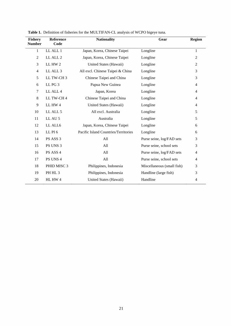
21

Table 1. Definition of fisheries for the MULTIFAN-CL analysis of WCPO bigeye tuna.

Fishery Number

Reference Code

Nationality Gear Region

1 LL ALL 1 Japan, Korea, Chinese Taipei Longline 1

2 LL ALL 2 Japan, Korea, Chinese Taipei Longline 2

3 LL HW 2 United States (Hawaii) Longline 2

4 LL ALL 3 All excl. Chinese Taipei & China Longline 3

5 LL TW-CH 3 Chinese Taipei and China Longline 3

6 LL PG 3 Papua New Guinea Longline 4

7 LL ALL 4 Japan, Korea Longline 4

8 LL TW-CH 4 Chinese Taipei and China Longline 4

9 LL HW 4 United States (Hawaii) Longline 4

10 LL ALL 5 All excl. Australia Longline 5

11 LL AU 5 Australia Longline 5

12 LL ALL6 Japan, Korea, Chinese Taipei Longline 6

13 LL PI 6 Pacific Island Countries/Territories Longline 6

14 PS ASS 3 All Purse seine, log/FAD sets 3

15 PS UNS 3 All Purse seine, school sets 3

16 PS ASS 4 All Purse seine, log/FAD sets 4

17 PS UNS 4 All Purse seine, school sets 4

18 PHID MISC 3 Philippines, Indonesia Miscellaneous (small fish) 3

19 PH HL 3 Philippines, Indonesia Handline (large fish) 3

20 HL HW 4 United States (Hawaii) Handline 4

22

Table 2. Main structural assumptions of the bigeye tuna base-case (GLM-MFIX) analysis, and details of estimated parameters, priors and bounds. Note that the number of estimated parameters shown is substantially greater than the effective number of parameters in a statistical sense because of the effects of priors, bounds and smoothing penalties.

Prior Bounds Category Assumptions Estimated parameters (ln = log transformed parameter)

No.µ σ Low High

Observation model for total catch data

Observation errors small, equivalent to a residual SD on the log scale of 0.07.

None na na na na na

Observation model for length-frequency data

Normal probability distribution of frequencies with variance determined by effective sample size and observed frequency. Effective sample size assumed to be 0.1 times actual sample size for all fisheries with a maximum effective sample size of 100.

None na na na na na

Observation model for weight-frequency data

Normal probability distribution of frequencies, variance determined by effective sample size and observed frequency. Effective sample size assumed to be equal to 0.1 times the actual sample size for all fisheries with a maximum effective sample size of 100.

None na na na na na

Observation model for tagging data

Tag numbers in a stratum have negative binomial probability distribution, with estimated variance parameters for fishery groups.

Variance parameters 4 - - 0 100

LL 1−LL6, CH/TW LL, PNG LL, PI LL

10 0.5 0.7 0.001 0.9

AU LL, HW LL, HW HL 4 0.8 0.7 0.001 0.9 PS 2 0.42 0.1 0.001 0.9

Tag reporting Purse seine reporting rates constrained to be equal within regions. PH /ID fishery reporting rates constrained to be equal. All reporting rates constant over time.

PH, ID fisheries 1 0.6 0.1 0.001 0.9 Tag mixing Tags assumed to be randomly mixed at the model region level two

quarters following the quarter of release. None na na na na na

Average spatially aggregated recruitment (ln)

1 - - -20 20

Spatially aggregated recruitment deviations (ln)

212 SRR 0.7 -20 20

Average spatial distribution of recruitment

5 - - 0 1

Recruitment Occurs as discrete events at the start of each quarter. Spatially-aggregated recruitment is weakly related to spawning biomass in the prior quarter via a Beverton-Holt SRR (beta prior for steepness with mode at 0.85 and SD of 0.16, lower bound 0.2) .The spatial distribution of recruitment in each quarter is allowed to vary with a small penalty on deviations from the average spatial distribution.

Time series deviations from average spatial distribution (ln)

1,054 0 1 -3 3

23

Initial population A function of the initial recruitment and equilibrium age structure in each region, which is in turn assumed to arise from the total mortality estimated for 1950−54 and movement rates.

Initial recruitment scaling (ln) 1 - - -8 8

Mean length age class 1 1 - - 20 40 Mean length age class 40 1 - - 140 200 von Bertalanffy K 1 - - 0 0.3 Independent mean lengths 7 0 0.7 Length-at-age SD 1 - - 3 10

Age and growth 40 quarterly age-classes, with the last representing a plus group. Juvenile age-classes 1-8 have independent mean lengths constrained by a small penalty for deviation from the von Bertalanffy growth curve; adult age-class mean lengths constrained by VB curve. SD of length-at-age are log-linearly related to the mean length-at-age. Mean weights ( jW ) computed internally by estimating the distribution of weight-at-age from the distribution of length-at-age and applying the weight-length relationship baLW = (a=0.0000210132, b=3.0 independently estimated from available length-weight data).

Dependency on mean length (ln) 1 - - -1.00 1.00

Selectivity Constant over time. Various smoothing penalties applied. Coefficients for the last 4 age-classes are constrained to be equal. Longline selectivities are non-decreasing with increasing age. Longline fisheries L2-L5 share selectivity parameters.

Selectivity coefficients (5 cubic spline nodes per fishery)

100 - - 0 1

Average catchability coefficients (ln)

15 - - -15 1

Seasonality amplitude (ln) 18 0 2.2 - - Seasonality phase 18 - - - - Catchability deviations PH/ID (ln) 34 0 0.1 -0.8 0.8

Catchability Constant over years and among regions for longline fisheries (effort data are scaled to reflect different region sizes). Seasonal variation for all fisheries apart from Philippines and Indonesian fisheries. Non-longline fisheries and the Australian and Taiwanese/Chinese longline fisheries have structural time-series variation, with random steps (catchability deviations) taken every 2 years.

Catchability deviations other (ln) 122 0 0.7 -0.8 0.8

Effort deviations LL 1, 2, 4, 7, 10, 12 (ln)

1,262 0 0.16 -6 6

Effort deviations PH, ID (ln) 280 0 0.22 -6 6

Fishing effort Variability of effort deviations constrained by a prior distributions. SD inversely proportional to the square root of normalised effort.

Effort deviations other (ln) 1,022 0 0.7 -6 6

Average natural mortality (ln) 0 - - - - Natural mortality Age-dependent but constant over time and among regions. Age-specific deviations (ln) 0 0 0.22 -5 5 Movement coefficients 56 0 0.32 0 3 Movement Age-dependent and varies by quarter but constant among years. No age-

dependent variation. Age-dependent component (ln) 0 0 0.32 -4 4

24

Table 3. Details of objective function components for the six analyses using alternative longline effort series (SHBS, GLM) and with either estimated (MEST) or fixed (MFIX) natural mortality-at-age.

Objective function component

SHBS-MEST

SHBS-MFIX

GLM-MEST

GLM-MFIX

FPOW-MEST

FPOW-MFIX

Total catch log-likelihood 481.78 486.09 421.09 429.2 415.57 416.53 Length frequency log-likelihood

-306,494.03 -306,527.50 -306,531.57 -306,502.73 -306,518.48 -306,491.01

Weight frequency log-likelihood

-492,292.57 -492,281.55 -492,238.44 -492,246.39 -492,258.35 -492,265.47

Tag log-likelihood 1,739.28 1,710.59 1,743.64 1,708.06 1,744.88 1,706.26 Penalties 6,820.44 6,896.80 4,548.56 4,598.85 4,518.59 4,585.10 Total function value -789,745.10 -789,715.57 -792,056.72 -792,013.01 -792,097.79 -792,048.59

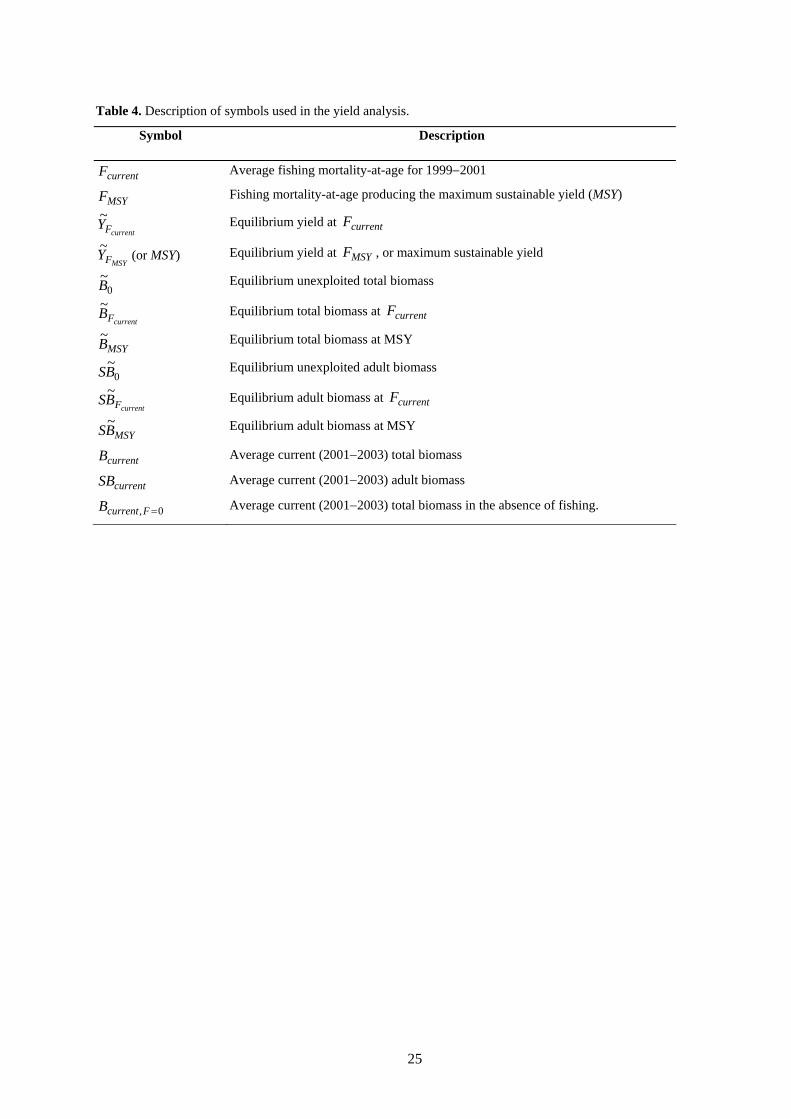
25

Table 4. Description of symbols used in the yield analysis.

Symbol Description

currentF Average fishing mortality-at-age for 1999−2001

MSYF Fishing mortality-at-age producing the maximum sustainable yield (MSY)

currentFY~ Equilibrium yield at currentF

MSYFY~ (or MSY) Equilibrium yield at MSYF , or maximum sustainable yield

0~B Equilibrium unexploited total biomass

currentFB~ Equilibrium total biomass at currentF

MSYB~ Equilibrium total biomass at MSY

0~BS Equilibrium unexploited adult biomass

currentFBS~ Equilibrium adult biomass at currentF

MSYBS~ Equilibrium adult biomass at MSY

currentB Average current (2001−2003) total biomass

currentSB Average current (2001−2003) adult biomass

0, =FcurrentB Average current (2001−2003) total biomass in the absence of fishing.

26

Table 5. Estimates of management quantities for the four analyses using alternative longline effort series. The highlighted rows are ratios of comparable quantities at the same point in time (black shading) and ratios of comparable equilibrium quantities (gray shading).

Management quantity

Units SHBS-MEST

SHBS-MFIX

GLM-MEST

GLM-MFIX

FPOW-MEST

FPOW-MFIX

currentFY~ t per quarter 17,500 17,520 19,060 16,240 15,800 16,800

MSYFY~ (or MSY) t per quarter 17,520 17,520 19,130 16,510 17,490 17,370

0~B t 798,800 738,300 670,300 658,400 776,300 707,600

currentFB~ t 324,600 269,200 277,900 197,400 226,800 195,200

MSYB~ t 355,400 269,200 259,500 239,500 332,700 269,300

0~BS t 406,300 440,500 348,300 392,600 395,900 421,500

currentFBS~ t 100,100 93,500 73,810 56,290 57,970 53,640

MSYBS~ t 115,100 93,500 64,730 78,780 103,700 92,710

currentB t 487,639 399,529 364,732 300,334 353,531 284,497

currentSB t 144,825 136,504 95,885 86,932 91,768 82,143

0, =FcurrentB t 951,542 1,019,768 840,672 920,945 818,593 906,588

0~BBcurrent 0.61 0.54 0.54 0.46 0.46 0.40

currentFcurrent BB ~ 1.50 1.48 1.31 1.52 1.56 1.46

MSYcurrent BB ~ 1.37 1.48 1.41 1.25 1.06 1.06

0, =Fcurrentcurrent BB 0.51 0.39 0.43 0.33 0.43 0.31

0~BSSBcurrent 0.36 0.31 0.28 0.22 0.23 0.19

currentFcurrent BSSB ~ 1.45 1.46 1.30 1.54 1.58 1.53

MSYcurrent BSSB ~ 1.26 1.46 1.48 1.10 0.88 0.89

0~~ BB

currentF 0.41 0.36 0.41 0.30 0.29 0.28

0~~ BSBS

currentF 0.25 0.21 0.21 0.14 0.15 0.13

0~~ BBMSY 0.44 0.36 0.39 0.36 0.43 0.38

0~~ BSBS MSY 0.28 0.21 0.19 0.20 0.26 0.22

MSYcurrent FF ~ 1.06 0.97 0.90 1.23 1.45 1.35

MSYF BBcurrent

~~ 0.91 1.00 1.07 0.82 0.68 0.72

MSYF BSBScurrent

~~ 0.87 1.00 1.14 0.71 0.56 0.58

MSYYcurrentF

~ 1.00 1.00 1.00 0.98 0.90 0.97

27

160°E120°E 140°E 180° 160°W 140°W

0°

10°S

20°S

10°N

Figure 1. Long-distance (>500 nmi) movements of tagged bigeye tuna.

1950 1960 1970 1980 1990 2000

020

4060

8010

012

0

Tota

l cat

ch (1

000s

mt)

LonglinePurse-seineOther

Figure 2. Total annual catch (1000s mt) of bigeye tuna from the WCPO by fishing method from 1952 to 2004. Data from 2004 are incomplete.

28

New spatial stratification 10

N30

N

120E 150E

30S

10S

180 150W 120W

R1

R3 R4

R5 R6

R2

Old spatial stratification

10N

30N

120E 150E

30S

10S

180 150W 120W

R1

R2 R3

R4 R5

Figure 3. Distribution of cumulative bigeye tuna catch from 1990−2004 by 5 degree squares of latitude and longitude and fishing gear; longline (blue), purse-seine (grey), and other (dark orange). The mamximum circle size represents a catch of 50,000 t. The grey lines indicate the spatial stratification used in 2005 assessment (upper panel) and the 2004 assessment (lower panel).

29

1950 1960 1970 1980 1990 2000

010

2030

4050

60

Region 1

LonglinePurse-seineOther

1950 1960 1970 1980 1990 2000

010

2030

4050

60

Region 2

1950 1960 1970 1980 1990 2000

010

2030

4050

60

Region 3

1950 1960 1970 1980 1990 2000

010

2030

4050

60

Region 4

1950 1960 1970 1980 1990 2000

010

2030

4050

60

Region 5

1950 1960 1970 1980 1990 2000

010

2030

4050

60

Region 6

Tota

l cat

ch (1

000s

mt)

Figure 4. Total annual catch (1000s mt) of bigeye tuna by fishing method and MFCL region from 1952 to 2004. Data from 2004 are incomplete.

30

Figure 5. Annual catches, by fishery. Circles are observed and the lines are model predictions. Units are catch number in thousands for the longline fisheries and thousand metric tonnes for all other fisheries.

31

Figure 6. Catch-per-unit-effort (CPUE) by fishery. Units are catch number per GLM-standardised effort (fisheries LL ALL 1−LL ALL 6), catch number per 100 nominal hooks (LL HW, CH/TW LL, LL PI, LL PG) and catch (t) per day fished/searched (all PS fisheries). Note that CPUE for PH RN, PH HL and ID are arbitrary and not based on data (see discussion on catchability and effort deviation constraints for these fisheries).

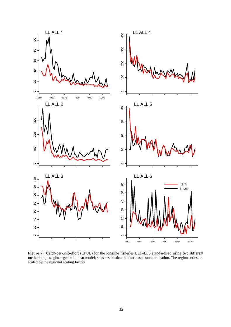
32

Figure 7. Catch-per-unit-effort (CPUE) for the longline fisheries LL1−LL6 standardised using two different methodologies. glm = general linear model; shbs = statistical habitat-based standardisation. The region series are scaled by the regional scaling factors.

33

Figure 8. Number of fish size measurements by year for each fishery. The upper black bars represent length measurements and the lower grey bars represent weight measurements. The sample size corresponding to the maximum bar length for each fishery is given on the right-hand side. The extent of the horizontal lines indicates the period over which each fishery occurred.

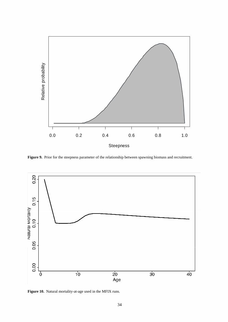
34

0.0 0.2 0.4 0.6 0.8 1.0

Steepness

Rel

ativ

e pr

obab

ility

Figure 9. Prior for the steepness parameter of the relationship between spawning biomass and recruitment.

Figure 10. Natural mortality-at-age used in the MFIX runs.

35

Figure 11. Residuals of ln (total catch) for each fishery (GLM-MFIX model). The dark line represents a lowess smoothed fit to the residuals.

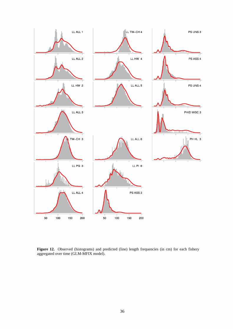
36

Figure 12. Observed (histograms) and predicted (line) length frequencies (in cm) for each fishery aggregated over time (GLM-MFIX model).

37

Figure 13. Observed (histograms) and predicted (line) weight frequencies (in kg) for each fishery aggregated over time (GLM-MFIX model).

38

Figure 14. Residuals (observed – predicted) of the aggregated proportion of fish in the larger length classes from sampled and predicted catches by fishery and sample period (GLM-MFIX model). The aggregated length range is 125–170 cm for all the longline fisheries and 70–120 cm for all other fisheries. The line represents a lowess smoothed fit to the data.

39

Figure 15. Residuals (observed – predicted) of the aggregated proportion of fish in the larger weight classes (35–70 kg) from sampled and predicted catches by fishery and sample period (GLM-MFIX model). The line represents a lowess smoothed fit to the data.

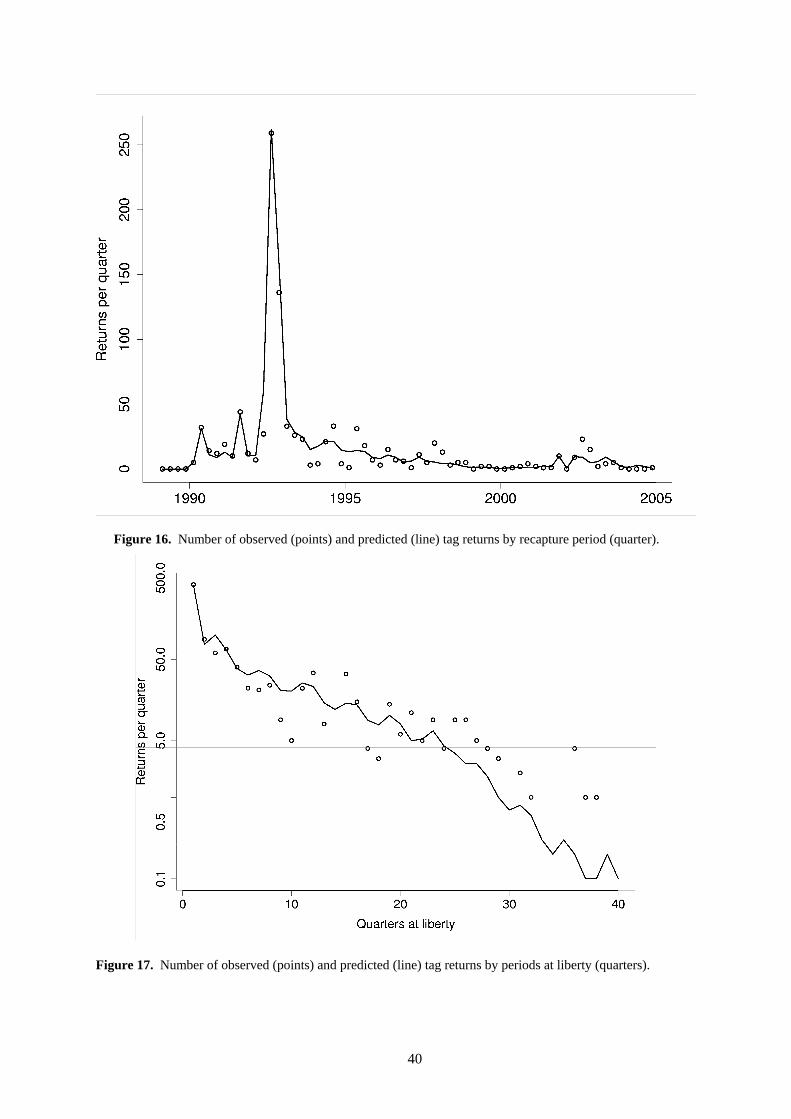
40

Figure 16. Number of observed (points) and predicted (line) tag returns by recapture period (quarter).

Figure 17. Number of observed (points) and predicted (line) tag returns by periods at liberty (quarters).

41

Figure 18. Number of observed (points) and predicted (line) tag returns by recapture period (quarter) for the various fisheries (or groups of fisheries) defined in the model. Only non-zero observations are plotted.

42

Figure 19. Effort deviations by time period for each fishery (GLM-MFIX model). For fisheries with longer time series, the dark line represents a lowess smoothed fit to the effort deviations.

43

Figure 20. Estimated mean lengths-at-age (heavy line) and the variability of length-at-age (shaded area represents ± 2 SD) (GLM-MFIX model). Age is in quarters and length is in cm (top figure). For comparison, length at age estimates are presented from tag release and recapture data (middle figure) and empirical age determination from otolith readings (bottom figure). The tagging data is presented as a linear growth vector (depicted as an arrow) from length at release to length at recovery. Only fish at liberty for at least 150 days are included. Age at release is assumed from the estimated growth function.

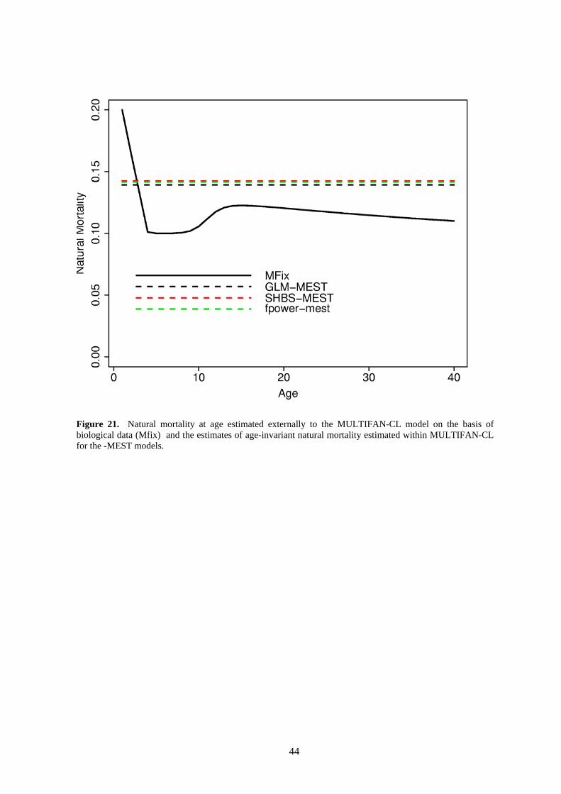
44

Figure 21. Natural mortality at age estimated externally to the MULTIFAN-CL model on the basis of biological data (Mfix) and the estimates of age-invariant natural mortality estimated within MULTIFAN-CL for the -MEST models.

45

R1 R2

R3 R4

R5 R6

Quarter 1R1 R2

R3 R4

R5 R6

Quarter 2

R1 R2

R3 R4

R5 R6

Quarter 3R1 R2

R3 R4

R5 R6

Quarter 4

Figure 22. Estimated quarterly movement coefficients at age (1, 10, 20, 30 quarters) from the GLM-MFIX model. The movement coefficient is proportional to the length of the arrow and increased weight of the arrow represents increasing age. The maximum movement (quarter 1, region 6 to region 4) represents movement of 12% of the fish at the start of the quarter.

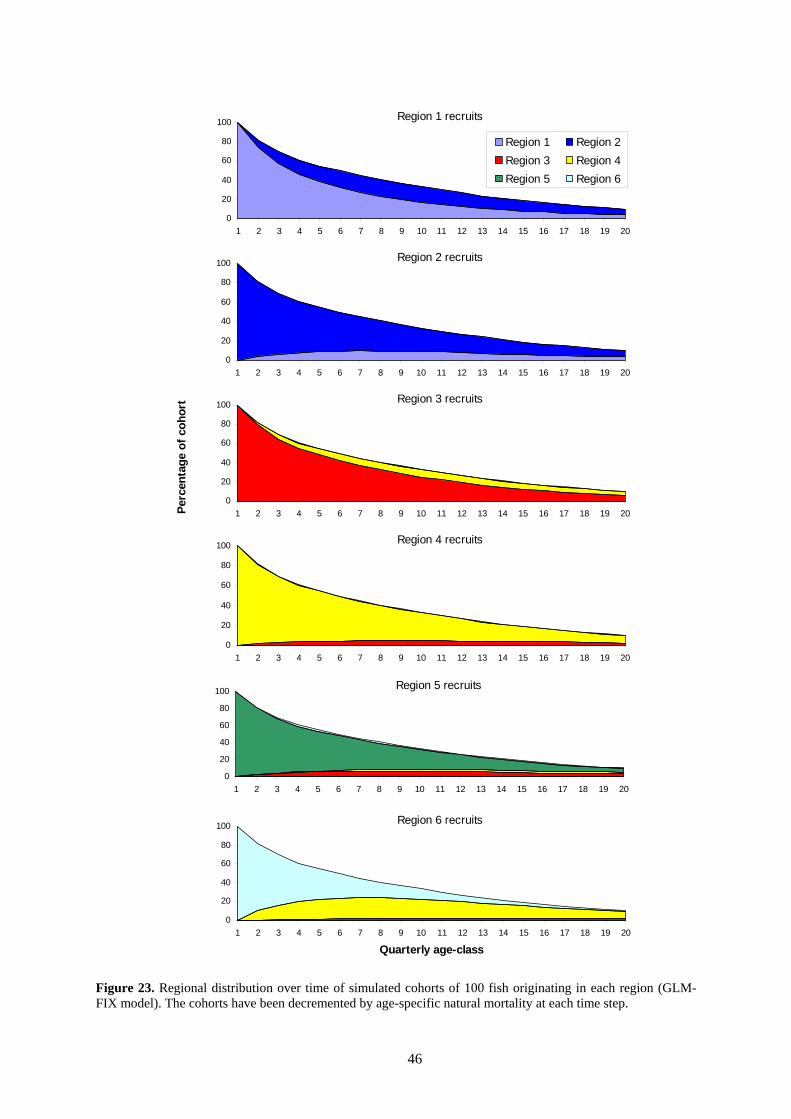
46

0

20

40

60

80

100

1 2 3 4 5 6 7 8 9 10 11 12 13 14 15 16 17 18 19 20

Region 1 Region 2Region 3 Region 4Region 5 Region 6

Region 1 recruits

0

20

40

60

80

100

1 2 3 4 5 6 7 8 9 10 11 12 13 14 15 16 17 18 19 20

Region 2 recruits

0

20

40

60

80

100

1 2 3 4 5 6 7 8 9 10 11 12 13 14 15 16 17 18 19 20

Region 3 recruits

0

20

40

60

80

100

1 2 3 4 5 6 7 8 9 10 11 12 13 14 15 16 17 18 19 20

Region 4 recruits

Perc

enta

ge o

f coh

ort

0

20

40

60

80

100

1 2 3 4 5 6 7 8 9 10 11 12 13 14 15 16 17 18 19 20

Region 5 recruits

0

20

40

60

80

100

1 2 3 4 5 6 7 8 9 10 11 12 13 14 15 16 17 18 19 20

Quarterly age-class

Region 6 recruits

Figure 23. Regional distribution over time of simulated cohorts of 100 fish originating in each region (GLM-FIX model). The cohorts have been decremented by age-specific natural mortality at each time step.

47

Figure 24. Selectivity coefficients, by fishery (GLM-MFIX model).

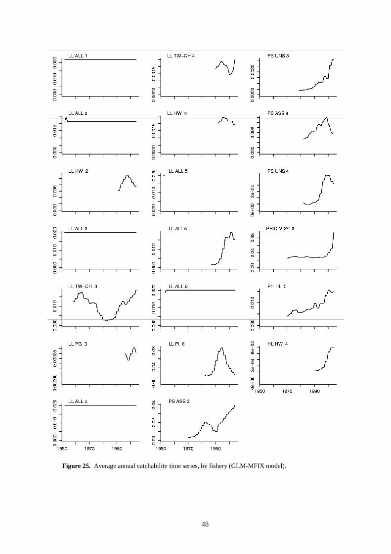
48

Figure 25. Average annual catchability time series, by fishery (GLM-MFIX model).

49

Figure 26. Estimated tag-reporting rates by fishery (black circles) (GLM-MFIX model). The white diamonds indicate the modes of the priors for each reporting rate and the grey bars (truncated at zero and 0.9, which were the bounds of the parameter estimates) indicate a range of ±1 prior SD.

50

Figure 27. Estimated annual recruitment (millions) by region and for the WCPO (GLM-MFIX model). The shaded area for the WCPO indicates the approximate 95% confidence intervals.

51

Figure 28. Estimated annual recruitment (millions of fish) for the WCPO obtained from the six different model options.

52

Figure 29. Estimated annual average total biomass (thousand t) by region and for the WCPO (GLM-MFIX model). The shaded areas indicate the approximate 95% confidence intervals.

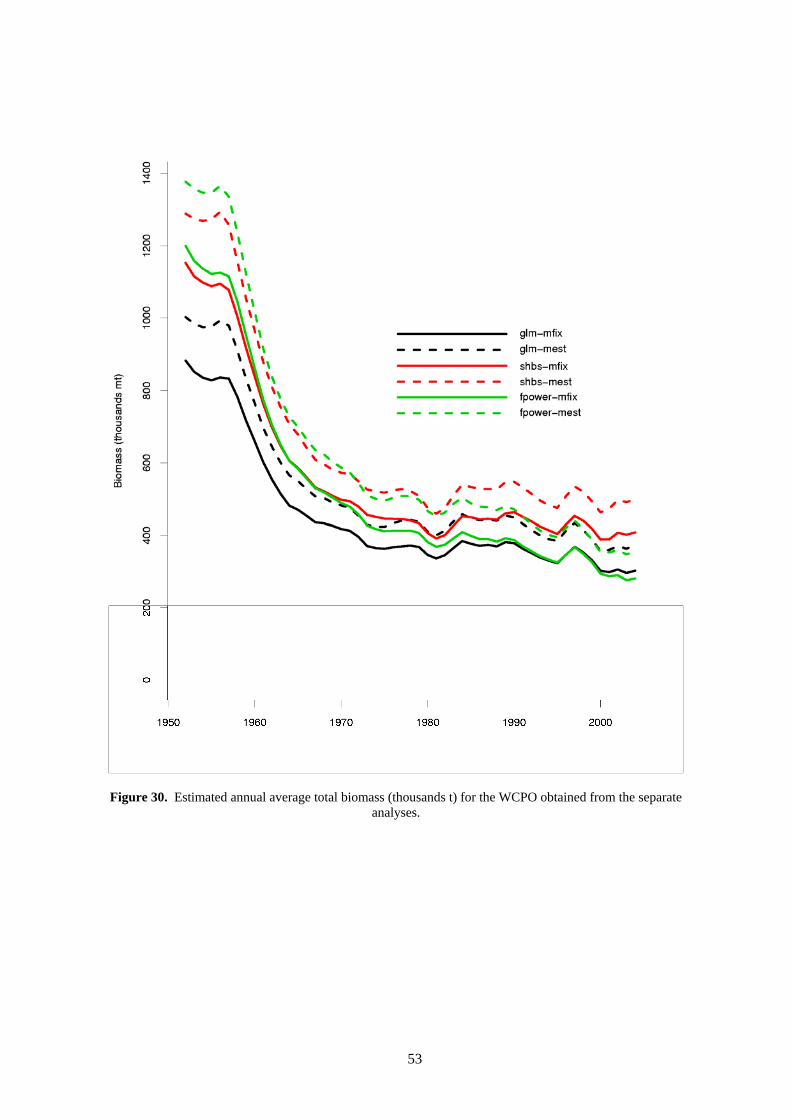
53

Figure 30. Estimated annual average total biomass (thousands t) for the WCPO obtained from the separate analyses.

54

Figure 31. A comparison of longline exploitable biomass by quarter and region (red line) and the quarterly standardised CPUE indices for the fisheries. For comparison, both series are scaled to the average of the series.

55

0.0

0.5

1.0

1.5

2.0

2.5

3.0

1 2 3 4 5 6

Region

Rel

ativ

e C

PUE/

expl

oita

ble

abun

danc

e CPUEExploitable abundance

Figure 32. CPUE and exploitable abundance for LL ALL 1−6 averaged over all time periods. Values for each region are scaled relative to their averages across all regions.

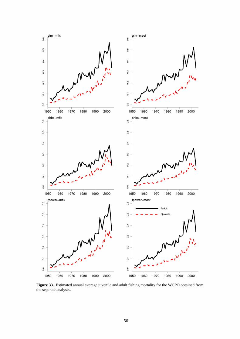
56

Figure 33. Estimated annual average juvenile and adult fishing mortality for the WCPO obtained from the separate analyses.

57

Figure 34. Estimated proportion at age (quarters) for the WCPO bigeye population (left) and fishing mortality at age (right) by year at decade intervals.

58

Figure 35. Comparison of the estimated biomass trajectories (lower heavy lines) with biomass trajectories that would have occurred in the absence of fishing (upper dashed lines) for each region and for the WCPO (GLM-MFIX model).

59

Figure 36. Ratios of exploited to unexploited total biomass (Bt/B0,t) for each region and the WCPO (GLM-MFIX model).

60

Figure 37. Ratios of exploited to unexploited total biomass (Bt/B0,t) for the WCPO obtained from the separate analyses.

61

1950 1960 1970 1980 1990 2000

020

4060

Region 1

1950 1960 1970 1980 1990 2000

010

2030

4050 Region 2

1950 1960 1970 1980 1990 2000

020

4060

80 Region 3

1950 1960 1970 1980 1990 20000

2040

6080 Region 4

1950 1960 1970 1980 1990 2000

020

4060

80

Region 5

1950 1960 1970 1980 1990 2000

010

3050

Region 6

1950 1960 1970 1980 1990 2000

020

4060

80 WCPO

Impa

ct %

PH/IDPS assocPS unassocLL

Figure 38. Estimates of reduction in spawning biomass due to fishing (fishery impact = 1-SBt/SB0,t) by region and for the WCPO attributed to various fishery groups (GLM-MFIX model). LL = all longline fisheries; PH/ID = Philippines and Indonesian domestic fisheries; PS assoc = purse seine log and FAD sets; PS unassoc = purse seine school sets.

62

1950 1960 1970 1980 1990 2000

010

2030

4050 Region 1

1950 1960 1970 1980 1990 2000

010

2030

Region 2

1950 1960 1970 1980 1990 2000

020

4060

80

Region 3

1950 1960 1970 1980 1990 20000

2040

60 Region 4

1950 1960 1970 1980 1990 2000

010

2030

4050 Region 5

1950 1960 1970 1980 1990 2000

010

2030

Region 6

1950 1960 1970 1980 1990 2000

010

3050

70

WCPO

Impa

ct %

PH/IDPS assocPS unassocLL

Figure 39. Estimates of reduction in total biomass due to fishing (fishery impact = 1-Bt/B0,t) by region and for the WCPO attributed to various fishery groups (GLM-MFIX model). LL = all longline fisheries; PH/ID = Philippines and Indonesian domestic fisheries; PS assoc = purse seine log and FAD sets; PS unassoc = purse seine school sets.

63

Figure 40. Estimated relationship between equilibrium recruitment and equilibrium spawning biomass (GLM-MFIX model). The grey area indicates the 95% confidence region. Estimated recruitment-spawning biomass points are plotted as open circles.

64

Figure 41. Yield (top), equilibrium biomass (middle) and equilibrium spawning biomass (bottom) as a function of fishing mortality multiplier (F-mult) obtained from the separate analyses. The estimate of SRR steepness associated with each analysis is provided in parentheses in the legend.

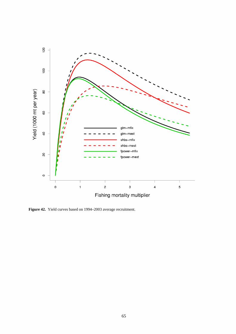
65

Figure 42. Yield curves based on 1994–2003 average recruitment.

66

Figure to come

Figure 43. Probability distribution of MSYcurrent FF ~ based on the likelihood profile method for the GLM-

MFIX model.

67

Figure 44. Probability distribution of MSYcurrent BB ~ based on the likelihood profile method for the GLM-

MFIX model.

68

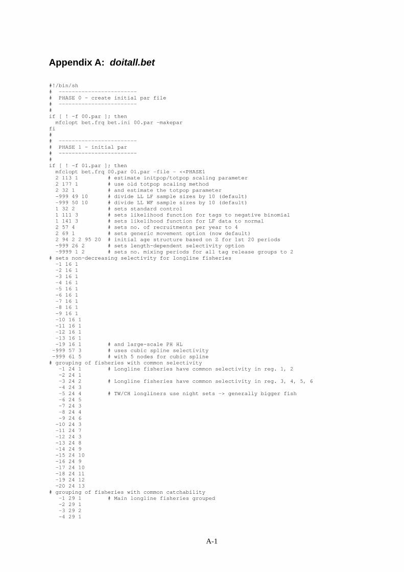
A-1

Appendix A: doitall.bet #!/bin/sh # ------------------------ # PHASE 0 - create initial par file # ------------------------ # if [ ! -f 00.par ]; then mfclopt bet.frq bet.ini 00.par -makepar fi # # ------------------------ # PHASE 1 - initial par # ------------------------ # if [ ! -f 01.par ]; then mfclopt bet.frq 00.par 01.par -file - <<PHASE1 2 113 1 # estimate initpop/totpop scaling parameter 2 177 1 # use old totpop scaling method 2 32 1 # and estimate the totpop parameter -999 49 10 # divide LL LF sample sizes by 10 (default) -999 50 10 # divide LL WF sample sizes by 10 (default) 1 32 2 # sets standard control 1 111 3 # sets likelihood function for tags to negative binomial 1 141 3 # sets likelihood function for LF data to normal 2 57 4 # sets no. of recruitments per year to 4 2 69 1 # sets generic movement option (now default) 2 94 2 2 95 20 # initial age structure based on Z for 1st 20 periods -999 26 2 # sets length-dependent selectivity option -9999 1 2 # sets no. mixing periods for all tag release groups to 2 # sets non-decreasing selectivity for longline fisheries -1 16 1 -2 16 1 -3 16 1 -4 16 1 -5 16 1 -6 16 1 -7 16 1 -8 16 1 -9 16 1 -10 16 1 -11 16 1 -12 16 1 -13 16 1 -19 16 1 # and large-scale PH HL -999 57 3 # uses cubic spline selectivity -999 61 5 # with 5 nodes for cubic spline # grouping of fisheries with common selectivity -1 24 1 # Longline fisheries have common selectivity in reg. 1, 2 -2 24 1 -3 24 2 # Longline fisheries have common selectivity in reg. 3, 4, 5, 6 -4 24 3 -5 24 4 # TW/CH longliners use night sets -> generally bigger fish -6 24 5 -7 24 3 -8 24 4 -9 24 6 -10 24 3 -11 24 7 -12 24 3 -13 24 8 -14 24 9 -15 24 10 -16 24 9 -17 24 10 -18 24 11 -19 24 12 -20 24 13 # grouping of fisheries with common catchability -1 29 1 # Main longline fisheries grouped -2 29 1 -3 29 2 -4 29 1

A-2

-5 29 3 -6 29 4 -7 29 1 -8 29 5 -9 29 6 -10 29 1 -11 29 7 -12 29 1 -13 29 8 -14 29 9 -15 29 10 -16 29 11 -17 29 12 -18 29 13 -19 29 14 -20 29 15 -1 60 1 -2 60 1 -3 60 2 -4 60 1 -5 60 3 -6 60 4 -7 60 1 -8 60 5 -9 60 6 -10 60 1 -11 60 7 -12 60 1 -13 60 8 -14 60 9 -15 60 10 -16 60 11 -17 60 12 -18 60 13 -19 60 14 -20 60 15 # grouping of fisheries for tag return data -1 32 1 -2 32 2 -3 32 3 -4 32 4 -5 32 5 -6 32 6 -7 32 7 -8 32 8 -9 32 9 -10 32 10 -11 32 11 -12 32 12 -13 32 13 -14 32 14 # PS assoc. and unassoc. returns are grouped -15 32 14 -16 32 15 -17 32 15 -18 32 16 # PH/ID returns returns are grouped -19 32 16 -20 32 17 # grouping of fisheries with common tag-reporting rates - as for tag grouping -1 34 1 -2 34 2 -3 34 3 -4 34 4 -5 34 5 -6 34 6 -7 34 7 -8 34 8 -9 34 9 -10 34 10 -11 34 11 -12 34 12 -13 34 13 -14 34 14 # PS assoc. and unassoc. returns are grouped -15 34 14 -16 34 15 -17 34 15 -18 34 16 # PH/ID returns returns are grouped

A-3

-19 34 16 -20 34 17 # sets penalties on tag-reporting rate priors -1 35 1 # The penalties are set to be small for LL fisheries -2 35 1 -3 35 50 # HI LL fishery thought to be high rep. rate -4 35 1 -5 35 1 -6 35 1 -7 35 1 -8 35 1 -9 35 50 -10 35 1 -11 35 50 # AU LL region 4 thought to be high rep. rate -12 35 1 -13 35 1 -14 35 50 # WTP PS based on tag seeding -15 35 50 -16 35 50 -17 35 50 -18 35 50 # PH/ID based on high recovery rate -19 35 50 -20 35 50 # HI HL thought to be high rep. rate # sets prior means for tag-reporting rates -1 36 50 # Mean of 0.5 and penalty of 1 -> uninformative prior -2 36 50 -3 36 80 # HI LL -4 36 50 -5 36 50 -6 36 50 -7 36 50 -8 36 50 -9 36 80 -10 36 50 -11 36 80 # AU LL region 4 -12 36 50 -13 36 50 -14 36 45 # WTP PS based on tag seeding and discounted for unable returns -15 36 45 -16 36 45 -17 36 45 -18 36 60 # PH/ID -19 36 60 # PH HL -20 36 80 # HI HL # sets penalties for effort deviations (negative penalties force effort devs # to be zero when catch is unknown) -999 13 -10 # higher for longline fisheries where effort is standardized -1 13 -50 -2 13 -50 -4 13 -50 -7 13 -50 -10 13 -50 -12 13 -50 -18 13 1 # sets penalties for catchability deviations -18 15 1 # low penalty for PH.ID MISC. -999 33 1 # estimate tag-reporting rates 1 33 90 # maximum tag reporting rate for all fisheries is 0.9 PHASE1 fi # --------- # PHASE 2 # --------- if [ ! -f 02.par ]; then mfclopt bet.frq 01.par 02.par -file - <<PHASE2 1 149 400 # set penalty on recruitment devs to 400/10 -999 3 37 # all selectivities equal for age class 37 and older -999 4 4 # possibly not needed -999 21 4 # possibly not needed 1 189 1 # write graph.frq (obs. and pred. LF data) 1 190 1 # write plot.rep 1 1 200 # set max. number of function evaluations per phase to 100 1 50 -2 # set convergence criterion to 1E+01 -999 14 10 # Penalties to stop F blowing out PHASE2 fi

A-4

# --------- # PHASE 3 # --------- if [ ! -f 03.par ]; then mfclopt bet.frq 02.par 03.par -file - <<PHASE3 2 70 1 # activate parameters and turn on 2 71 1 # estimation of temporal changes in recruitment distribution PHASE3 fi # --------- # PHASE 4 # --------- if [ ! -f 04.par ]; then mfclopt bet.frq 03.par 04.par -file - <<PHASE4 2 68 1 # estimate movement coefficients PHASE4 fi # --------- # PHASE 5 # --------- if [ ! -f 05.par ]; then mfclopt bet.frq 04.par 05.par -file - <<PHASE5 1 16 1 # estimate length dependent SD PHASE5 fi # --------- # PHASE 6 # --------- if [ ! -f 06.par ]; then mfclopt bet.frq 05.par 06.par -file - <<PHASE6 1 173 8 # estimate independent mean lengths for 1st 8 age classes 1 182 10 PHASE6 fi # --------- # PHASE 7 # --------- if [ ! -f 07.par ]; then mfclopt bet.frq 06.par 07.par -file - <<PHASE7 -999 27 1 # estimate seasonal catchability for all fisheries -18 27 0 # except those where -19 27 0 # only annual catches PHASE7 fi # --------- # PHASE 8 # --------- if [ ! -f 08.par ]; then mfclopt bet.frq 07.par 08.par -file - <<PHASE8 -3 10 1 # estimate -5 10 1 # catchability -6 10 1 # time-series -8 10 1 # for all -9 10 1 # non-longline -11 10 1 # fisheries -13 10 1 -14 10 1 -15 10 1 -16 10 1 -17 10 1 -18 10 1 -19 10 1 -20 10 1 -999 23 23 # and do a random-walk step every 23+1 months PHASE8 fi # --------- # PHASE 9 # --------- if [ ! -f 09.par ]; then mfclopt bet.frq 08.par 09.par -file - <<PHASE9 1 14 1 # estimate von Bertalanffy K 1 12 1 # and mean length of age 1 PHASE9 fi # ---------

A-5

# PHASE 10 # --------- if [ ! -f 10.par ]; then mfclopt bet.frq 09.par 10.par -file - <<PHASE10 # grouping of fisheries for estimation of negative binomial parameter a -1 44 1 -2 44 1 -3 44 1 -4 44 1 -5 44 1 -6 44 1 -7 44 1 -8 44 1 -9 44 1 -10 44 1 -11 44 1 -12 44 1 -13 44 1 -14 44 2 -15 44 2 -16 44 2 -17 44 2 -18 44 3 -19 44 3 -20 44 4 -999 43 1 # estimate a for all fisheries PHASE10 fi # --------- # PHASE 11 # --------- if [ ! -f 11.par ]; then mfclopt bet.frq 10.par 11.par -file - <<PHASE11 -100000 1 1 # estimate -100000 2 1 # time-invariant -100000 3 1 # distribution -100000 4 1 # of -100000 5 1 # recruitment -100000 6 1 PHASE11 fi # --------- # PHASE 12 # --------- if [ ! -f 12.par ]; then mfclopt bet.frq 11.par 12.par -file - <<PHASE12 2 145 5 1 149 0 2 146 1 2 147 1 2 148 16 2 155 4 2 153 31 2 154 16 1 1 3000 1 50 -3 PHASE12 fi

B-1

Appendix B: bet.ini # number of age classes 40 # maturity at age 0.0 0.0 0.0 0.0 0.0 0.0 0.0 0.0 0.0 0.0 0.05 0.1 0.2 0.4 0.6 0.7 0.8 0.85 0.9 0.95 1.0 1.0 1.0 1.0 1.0 1.0 1.0 1.0 1.0 1.0 1.0 1.0 1.0 1.0 1.0 1.0 1.0 1.0 1.0 1.0 # natural mortality 0.112828307 # movement map 1 2 3 4 # diffusion coffs 0.01 0.01 0.01 0.01 0.01 0.01 0.01 0.01 0.01 0.01 0.01 0.01 0.01 0.01 0.01 0.01 0.01 0.01 0.01 0.01 0.01 0.01 0.01 0.01 0.01 0.01 0.01 0.01 0.01 0.01 0.01 0.01 0.01 0.01 0.01 0.01 0.01 0.01 0.01 0.01 0.01 0.01 0.01 0.01 0.01 0.01 0.01 0.01 0.01 0.01 0.01 0.01 0.01 0.01 0.01 0.01 # age_pars (row 2 is for M-at-age specification) 0 0 0 0 0 0 0 0 0 0 0 0 0 0 0 0 0 0 0 0 0 0 0 0 0 0 0 0 0 0 0 0 0 0 0 0 0 0 0 0 0.57270008 0.388151602 0.169824717 -0.109880777 -0.120429055 -0.120184071 -0.119736681 -0.118950236 -0.117624734 -0.115488279 -0.112200121 -0.107371589 -0.100609865 -0.091587038 -0.080133729 -0.06684202 -0.051242744 -0.034614946 -0.018129082 -0.00301803 0.009741098 0.019643201 0.026664669 0.031113414 0.033443002 0.034116377 0.033536898 0.032027915 0.029837148 0.027150142 0.024104578 0.020802649 0.017320587 0.013715783 0.010031876 0.006302492 0.00255379 -0.001193612 -0.004923295 -0.008622116 0 0 0 0 0 0 0 0 0 0 0 0 0 0 0 0 0 0 0 0 0 0 0 0 0 0 0 0 0 0 0 0 0 0 0 0 0 0 0 0 0 0 0 0 0 0 0 0 0 0 0 0 0 0 0 0 0 0 0 0 0 0 0 0 0 0 0 0 0 0 0 0 0 0 0 0 0 0 0 0 0 0 0 0 0 0 0 0 0 0 0 0 0 0 0 0 0 0 0 0 0 0 0 0 0 0 0 0 0 0 0 0 0 0 0 0 0 0 0 0 0 0 0 0 0 0 0 0 0 0 0 0 0 0 0 0 0 0 0 0 0 0 0 0 0 0 0 0 0 0 0 0 0 0 0 0 0 0 0 0 0 0 0 0 0 0 0 0 0 0 0 0 0 0 0 0 0 0 0 0 0 0 0 0 0 0 0 0 0 0 0 0 0 0 0 0 0 0 0 0 0 0 0 0 0 0 0 0 0 0 0 0 0 0 0 0 0 0 0 0 0 0 0 0 0 0 0 0 0 0 0 0 0 0 0 0 0 0 0 0 0 0 0 0 0 0 0 0 0 0 0 0 0 0 0 0 0 0 0 0 0 0 0 0 0 0 0 0 0 0 0 0 0 0 0 0 0 0 0 0 0 0 0 0 0 0 0 0 0 0 0 0 0 0 0 0 0 0 0 0 0 0 0 0 0 0 0 0 0 0 0 0 0 0 0 0 0 0 0 0 # recruitment distribution 0.05 0.06 0.40 0.35 0.05 0.09 # The von Bertalanffy parameters 28.000000000000 20.000000000000 40.000000000000 180.000000000000 140.000000000000 200.000000000000 0.075000000000 0 0.300000000000 # Length-weight coefficients 2.10132e-05 3 # Variance parameters 6.000000000000 3.000000000000 12.000000000000 0.400000000000 -1.500000000000 1.500000000000 # The number of mean constraints 0