REPORT OF THE 2011 ICCAT YELLOWFIN TUNA STOCK ASSESSMENT ... · REPORT OF THE 2011 ICCAT YELLOWFIN...

YFT ASSESSMENT – SAN SEBASTIAN 2011

1

REPORT OF THE 2011 ICCAT YELLOWFIN TUNA STOCK ASSESSMENT SESSION

(San Sebastián, Spain - September 5 to 12, 2011) 1. Opening, adoption of agenda and meeting arrangements The Meeting was held at the INASMET-Tecnalia Center in San Sebastián from September 5 to 12, 2011. Dr. Josu Santiago (SCRS Chair), opened the meeting and welcomed participants (“the Working Group”). Dr. Craig Brown (USA), meeting Chairperson, welcomed meeting participants and thanked AZTI for hosting the meeting and providing all the logistical arrangements. Dr. Brown proceeded to review the Agenda which was adopted without changes (Appendix 1). The List of Participants is included in Appendix 2. The List of Documents presented at the meeting is attached as Appendix 3. The following participants served as Rapporteurs: Items 1, 9 and 10 P. Pallarés Item 2 H. Murua and D. Gaertner Items 3.1, 3.2 and 3.3 J. Ariz, A. Delgado de Molina, and A. Amorin Item 3.4 M. Ortiz and C. Palma Item 4 G. Díaz and P. De Bruyn Item 5.1, 6.1 and 7.1 D. Die, K. Satoh, H. Ijima, E. Chassot Item 5.2, 6.2 and 7.2 S. Cass-Calay Item 6.3 G. Scott and C. Brown Item 8 G. Scott and J. Santiago Coordinator of model inputs, figures and tables J. Walter 2. Review of Biological historical and new data Yellowfin tuna is a tropical and subtropical species distributed mainly in the epipelagic oceanic waters of the three oceans. The sizes exploited range from 30 cm to over 170 cm; maturity occurs at about 100 cm. Smaller fish (juveniles) form mixed schools with skipjack and juvenile bigeye, and are mainly limited to surface waters; while larger fish form schools in surface and sub-surface waters. Reproductive output among females has been shown to be highly variable. The main spawning ground is the equatorial zone of the Gulf of Guinea, with spawning primarily occurring from January to April. Juveniles are generally found in coastal waters off Africa. In addition, spawning occurs in the Gulf of Mexico, in the southeastern Caribbean Sea, and off Cape Verde, although the relative importance of these spawning grounds is unknown. Although such separate spawning areas might imply separate stocks or substantial heterogeneity in the distribution of yellowfin tuna, a single stock for the entire Atlantic is assumed as a working hypothesis, taking into account that data indicates yellowfin is distributed continuously throughout the entire tropical Atlantic Ocean and tag are recovered on a regular base from west to east. Males are predominant in the catches of larger sized fish. Natural mortality is assumed to be higher for juveniles than for adults as showed from tagging studies in other oceans. The natural mortality rates have been showed to be size-dependant in bigeye, skipjack and yellowfin tuna in the western tropical Pacific Ocean using tagging data (Hampton, 2000). In summary, this work demonstrated that M was an order of magnitude higher in the smallest size-class in comparison to fish of midsized. Moreover, it showed that mortality changed from high to low around 40 cm FL, approximately the size at which the three species recruit to the PS fishery in the western Pacific. The results of this work underline the importance of accounting for size- or age-specific natural mortality rates. In that sense, variable mortality for yellowfin was discussed by the group and it was agreed to continue using variable M in the assessment. Growth rates have been described as relatively slow initially, increasing at the time the fish leave the nursery grounds. Nevertheless, questions remain concerning the most appropriate growth model for Atlantic yellowfin tuna. A recent study (Shuford et al., 2007) developed a new growth curve using daily growth increment counts from otoliths. The results of this study, along with other recent hard part analyses, did not support the concept of the two-stanza growth model (initial slow growth) which is currently used for ICCAT yellowfin tuna stock assessments. This discrepancy should be addressed at inter-sessional meetings.


2

Only one document (SCRS/2011/141) on the biology of yellowfin was presented during the 2011 Working Group. This preliminary study, using pop-up tags, investigates the habitat use of yellowfin in the Gulf of Mexico. Yellowfin residence time at different depths depending on the difference between the temperature at depths and the surface were studied. Results show that yellowfin tuna spent 25.1% of time in the surface mixed layer in darkness, but only 4.3% during daylight hours. The ranges and means for the observed proportions of time spent at temperatures relative to the surface temperature were reflected in the observed percentage of time spent at depth, with greater exploration of deeper, colder waters during daylight periods. The majority of time was spent at depths shallower than 80 m. Although yellowfin tuna vertical distributions are influenced by temperature (other environmental factors also play a role), this study shows that yellowfin are able to tolerate cooler temperatures for brief periods during the day, which should be taken into account in the standardization of catch rates of different fleets for the assessment. The tabulated Delta-T percentiles reported in the document provide direct input variables required for habitat standardization models. The Group was also informed that NMFS laboratory in Miami is currently conducting electronic tagging experiments in the Gulf of Mexico. Large yellowfin (around 130 cm FL) were tagged with pop-up tags from longliners. Preliminary results showed different types of movements, including migration outside the Gulf of Mexico. The Group welcomes this type of studies and encourages the authors to continue and to present more conclusive results at future ICCAT tropical species working groups due to their importance for the understanding of stock structure, migration patterns, and other ecological characteristics of yellowfin in the Gulf of Mexico. The table below summarizes the biological parameters adopted by the SCRS and used in the 2011 Atlantic yellowfin assessments.

Parameter Yellowfin Natural mortality Assumed to be 0.8 for ages 0 and 1, and 0.6 for ages 2+

Assumed “birth date” of age 0 fish February 14 (approximate mid-point of the peak spawning season).

Plus group Age 5+

Growth rates

Length at age was calculated from the Gascuel et al. (1992) equation: FL (cm) = 37.8 + 8.93 * t + (137.0 – 8.93 * t) * [1 – exp(-0.808 * t)]7.49

Weights -at-age

Average weights-at-age were based on the Gascuel et al. (1992) growth equation and the Caveriviere (1976) length-weight relationship: W(kg) = 2.1527 x 10-5

* L(cm)2.976

Maturity schedule Assumed to be knife-edge at the beginning of age 3.

Partial recruitment Based on output from age-structured VPA (see section addressing yield-

per-recruit).

3. Review of fishery statistics: Effort and catch data, including size frequencies and fisheries trends The Secretariat presented, at the beginning of the meeting, updated (as of 2011-09-02) versions of Task I catch statistics and Task II size information of yellowfin tuna available in the ICCAT database. Some specific Task II catch and effort statistics (e.g., Dakar based BB fisheries, European PS fisheries by fishing mode FAD/FSC, etc.) were also prepared to be used in various studies. The information was revised by the Working Group, corrected whenever required, and used in the assessment 3.1 Description of fisheries Yellowfin tuna are caught in the entire tropical Atlantic, between 45ºN and 40ºS, by surface gears (purse seine, baitboat and handline) and by longline (Figures 1 and 2.). Table 1 presents the yellowfin landings by flag and gear.


3

− Baitboat

In the East Atlantic, the baitboat fisheries exploit concentrations of juvenile yellowfin in schools mixed with bigeye and skipjack. There are several baitboat fisheries that operate along the African coast. The most important, in terms of catch, is the Ghanaian baitboat fishery based at Tema. This fleet began to use FADs (fish aggregating device/floating object, which can be natural or artificial) in the early 1990s to enhance the capture of the species together with other tunas. Over 70-80% of these catches in recent years are on FADs; the mean weight of the captured fishes has remained relatively stable at around 2 kg (mode around 48cm). There is another baitboat fishery based in Dakar that began operation in 1956 in the coastal areas off Senegal and Mauritania. Other baitboat fisheries operate in the various archipelagos in the Atlantic (Azores, Madeira, Canary Islands and Cape Verde), which target different species of tuna, including yellowfin according to the season. The average weight of yellowfin tuna taken by these fleets is highly variable (between 7 and 30 kg); lengths range from 38 cm to 80 cm with the mode around 48 cm. Since the early 1990s, the fleets in Dakar and the Canary Islands have operated using a different method, i.e. using the boat as a FAD, to aggregate various species of tuna, including yellowfin tuna. In the West Atlantic, Venezuelan and Brazilian baitboats target yellowfin together with skipjack and other small tuna. The sizes of yellowfin are between 45cm and 175 cm for the Venezuelan fleet and from 45 to 115 cm, with the mode at 65 cm for the Brazilian fleet. − Purse seine The East Atlantic purse seine fisheries began in 1963 and developed rapidly in the mid-1970s. They initially operated in coastal areas and gradually extended to the high seas. Purse seiners catch large yellowfin in the Equatorial region in the first quarter of the year, coinciding with the spawning season and area. They also catch small yellowfin in association with skipjack and bigeye. Since the early 1990s, several purse seine fleets (France, Spain and associated fleets) have operated mainly on or associated with fishing aggregating devices (FADs), between 45 and 55% of the total purse seine catch being taken by this method, while previously, the proportion of the catch taken on natural floating objects was around 15% of the total purse seine catch. The Ghanaian purse seine fleet predominantly fishes off FADs (80%-85%) with fishing collaboration between the purse seine fleet and the baitboats. Frequently, FADs with accumulations of fish are first located by baitboats, who call in a purse seiner to make the set if the accumulation is large. In this situation, the catch is shared between the purse seiner and the baitboat. Although the fleets are fishing on floating objects throughout the year, the main catches occur in the first and fourth quarter of the year, with skipjack as the dominant species together with lesser quantities of yellowfin and bigeye. The species composition of the schools associated with floating objects is very different from that of free schools. Yellowfin catches from floating object represented between 14% and 21% of the total catch in the years between 1991 and 2010 (16% in 2010) for the French, Spanish and associated fleets. The East Atlantic purse seine fishery shows a bimodal distribution in the size classes for yellowfin, with modes near 50cm and 150 cm but with very few intermediate sizes and a high proportion of big fish (more than 160cm). The average weight of yellowfin tuna caught by the European and associated purse seine fleets was 9.4 kg in 2010 (3.1 kg with FADs and 30.4kg unassociated fishes). The sizes of yellowfin caught by the Ghanaian purse seiners has ranged around 48-52 cm for the recent decade. The catch series available for these stock assessments include catches of "faux poisson" (fish sold in the local markets of the landing ports, which are not reported in the manner of the rest of the catches). The "faux poisson" catches made by the European purse seine fleets from 1981 until now have been calculated by species and reported to ICCAT. In response to new developments in the purse seine fishery and to concerns over increased fishing mortality rate on bigeye tuna, a voluntary closed season/area for fishing with artificial FADs for a period of three months in a wide area of the equatorial Atlantic was implemented in 1997. In 1998 the Commission formally adopted the area closures [Rec. 98-01] and then extended the closure to all surface fleets in 1999 [Rec. 99-01]. Starting in 2005, those restrictions were discontinued, and instead a new management strategy (Piccolo) was established which prohibited all surface fishing in a much smaller area and only for the month of November [Rec. 04-01].


4

In the West Atlantic, Venezuela and Brazil have operated purse seine fisheries since 1970 off the coast of Venezuela and in the south of Brazil. Landings were sporadic in the 1970s but increased through the 80s and 90s and have generally been higher than western baitboat landings except in the most recent time period where they are approximately equal. Yellowfin size range caught by western Atlantic purse seiners (35 to 75 cm) is smaller compared to the eastern purse seiners, with the majority of fish being of intermediate size (mode 40 cm). − Longline The longline fishery began at the end of the 1950s and soon became important, with significant catches being taken by the early 1960s. Since then the catches have gradually decreased. Longline fisheries capturing yellowfin tuna are found throughout the Atlantic (Figure 2). The degree of targeting toward yellowfin varies across the longline fleets. In the Gulf of Mexico, both U.S. and Mexican longline vessels target yellowfin (the average weight of yellowfin was between 32 and 39 kg during the period from 1994 to 2006). Venezuelan vessels also target yellowfin, at least seasonally. In contrast, Japanese and Chinese Taipei vessels began in the mid-1970s and in the early-1980s to shift targeting away from yellowfin and albacore, respectively, toward bigeye tuna through the use of deep longline. Uruguayan longliners also capture yellowfin in the south western Atlantic, with FL sizes between 52 and 180 cm (mode at 110 cm or 26 kg; Domingo, et al, 2009). Since 2000, a small-size fleet off Cabo Frio City, Rio de Janeiro-RJ State, Brazil (22o to 24oS and 40o to 44oW) has started fishing. This fleet is growing in number and in 2010 it had about 350 boats, representing 15% of the RJ total yield. This fleet targets dolphinfish using different equipment and catches yellowfin mainly with handline (55%) and mid-water longline (8%) (SCRS/2011/143). 3.2 Catches The historical Task I catches have not undergone major updates since the 2010 SCRS. Only the most recent three years have changed slightly (< 1% in total) with various revisions made by several CPCs in accordance with the SCRS revision rules. Some provisional estimates of IUU since 2006, however, could add from 5,000 to 20,000 t per year to the overall catches in the recent past (SCRS/2011/016). 3.2.1 Yellowfin Table 1 and Figures 3 to 6 show the development of yellowfin catches in the total (by area and by gear), East and West Atlantic. Total Atlantic yellowfin catches in 2010 amounted to 108,343 t, in the East Atlantic was 86,133 t and in the West was 22,210 t. Yellowfin catches increased from 1950s to an average of 150,000 t in the 1980s, they reached the highest figure in 1990 with catches of 193,536 t. Since then the catches had gradually declined, with recent years being at a similar level to those at the beginning of the 1970s. In the recent years, several European purse seiners have returned to the Atlantic Ocean with a resulting increase in catches. − Baitboat Total catch by this gear for the whole Atlantic was 9,568 t in 2010, lower compared to the catch in 1993 of nearly 25,000 t. In the East Atlantic some fleets, with significant catches at the beginning of the fishery (22,135 t in 1968, e.g., Angola, Cape Verde or Japan), have decreased landings (8,132 t in 2010) In the West Atlantic (Figure 6) baitboat catches started in 1974, increased regularly from 1,300 t in 1974 to 7,000 t in 1994, and later decreased to about 1.450 t in 2010. − Purse seine Yellowfin catches by this fleet reached 74.172 t (68%) for the entire Atlantic in 2010. In the East Atlantic, catches increased rapidly in the early years of the fishery (Figure 5), from 10,000 t in the 1960s to 100,000 t in 1980, stabilizing at this level until 1983 followed by a sharp decrease in 1984 (74,173 t). This occurred as a result of the drastic decrease in effort which took place following the fall in yield of large sized yellowfin, mainly due to the French, Spanish and associated purse seine fleets abandoning the fishery. Catches later increased, with a record catch in 1990 of over 129,000 t, followed by a decreasing trend in subsequent years, reaching 58,319 t in 2006. In the follow years the catch increased again, reaching 69.953 t in 2010 due to re-


5

entry of purse-seine effort into the Atlantic. For the "faux poisson", the estimates corresponding to yellowfin show that the highest figure was 2,750 t in 1993, with 533 t in 2010. The Working Group on Ghanaian statistics, which met in 2011, provided new information on the Ghanaian fisheries trends. Based in the data provided by the Ghanaian scientists and with additional information from other sources, the Working Group was able to reconstruct detailed catch, effort and size data as well as detailed information on fleets and geographical distribution of catches. As an example, Figures 7 to 9 show the catch distribution of Ghanaian catches in the historical period (1969-1980), before the development of the FAD fishery, and in the recent period (2008-2010). These figures show the extension of the fishery from a coastal area to an area similar to that of the European and associated fisheries on FADs (Figure 10). Incomplete monitoring of the Ghanaian fleet catches since 2006 may have resulted in a potentially large underreporting of YFT catch. In the West Atlantic (Figure 6) catches increased since the beginning of the fishery in the early 1960s to 1983 when they reached 25,000 t. Catches in the following years show considerable variation as a part of this fleet moved to the Pacific Ocean. Caches in 2010 were 4,219 t. Most of the catch in the West Atlantic is taken by the Venezuelan purse seine fishery (in some years being 100% of the total catch). − Longline

After a maximum of over 50,000 t reached in 1959-1961, longline catches decreased to a level of around 30,000 t in the early 1970s. Longline catch levels in the 2000s have been about 23,000 t. Longline catches in 2010 reached 19,302 t. The main fisheries are those of Chinese Taipei, Japan, United States, Mexico and Brazil. The appearance of important catches, beginning in 1985, by NEI fleets in unknown areas is of concern as it is uncertain to what extent these catches actually occurred in the Atlantic. A multi-gear fleet in the western Atlantic fishing from Cabo Frio City, Rio de Janeiro, Brazil caught about 11 t of yellowfin in 2003. Catches increased to 183 t and 137 t in 2006 and 2007, respectively, and decreased to 8 t in 2010 (SCRS/2011/143). 3.3 Fishing effort

In general, in multi-species fisheries such as the surface tropical tunas fisheries, it is difficult to discriminate fishing effort by species. Beginning in the 1990s, important changes have taken place in the East Atlantic main surface fisheries which have further complicated the estimation of effective effort, including the greatly increased in the number of FADs used by purse seiners and baitboats, as well as the use of baitboats as floating objects. As indicators of the nominal effort in the East Atlantic, the carrying capacity of the purse seine and baitboat fleets has traditionally been used. Figure 11 shows the development of carrying capacity of the surface fleets in the East Atlantic for the period 1972-2010, including new information from Ghanaian fleets. The baitboat carrying capacity has remained stable since the late 1970s at around 10,000 t. The carrying capacity of the purse seine fleet, on the other hand, has undergone significant changes during the whole period under consideration, with a constant increase from the start of the fishery until 1983, when carrying capacity exceeded 70,000 t. After that, carrying capacity decreased considerably to 37,000 t in 1990, due in part to the fleet abandoning this fishery. There was a slight increase in the following two years (1991 and 1992) followed by a progressive decline, with capacity at around 29,700 t in the year 2006 and then an increase to 39,600 t between 2006 and 2010 due to movement of effort into the Atlantic mainly from the Indian Ocean (SCRS/2011/137, SCRS/2011/130, SCRS/2011/136). Document SCRS/2011/137 shows the development of both nominal fishing effort measures for EC and associated purse seiners: the number of 1-degree rectangles explored and the number with effort greater than 1 fishing day, and total purse seiners fishing days (1991-2010). It can be observed that, the searching area remained at the same level from 1991 until 2007, after which both searching area and the number of fishing days increased. For the West Atlantic, there have been substantial recent changes in the amount and distribution of fishing effort in the Brazilian longline fishery. Until 1995, sharks were the primary target species (58% of the total catches). However, since 1993, the proportion of sharks declined, being replaced by swordfish as the dominant species in this fishery (swordfish now represent 48% of the total catches). Effort in the Venezuelan surface fisheries has been high since 1992 (more than 8000 t vessel carrying capacity). Effort in the U.S. longline fishery, which is active in the north western Atlantic and in the Gulf of Mexico, has declined somewhat in the last few years.


6

Japanese longline effort for yellowfin tuna has also declined in recent years. This fleet mainly targets other species (bigeye and bluefin).In contrast, Venezuelan and Mexican longline effort for yellowfin tuna has increased in recent years. Effort in the multi-gear fleet fishing out of Rio de Janiero, Brazil is around 350 vessels (SCRS/2011/143). 3.4 CAS and CAA estimations The Secretariat presented at the beginning of the meeting, an update of the yellowfin catch-at-size (CAS) matrix estimations for the period 1970-2010. The standard proceedings and substitution rules were applied. As a standard procedure, the CAS output is standardised in 1 cm lower limit size frequencies, keeping always the maximum time-area granularity of the size information used. As recommended in the 2008 assessment, the period between 1975 and 1982 was revised and updated, in addition to the years 2007 to 2010. The remaining CAS series (periods 1970-1974 and 1983-2006) were revised and corrected to make the CAS weight equivalent with Task I (by year/fleet/gear/stock combinations). The yellowfin substitution tables (not here included given their sizes) used to build the yellowfin CAS, are available upon an explicit request to the Secretariat. A CAS revision of Japan was presented during the meeting (SCRS/2011/128) for the period 1995-2010. Upon a detailed explanation for such revision, the Working Group agreed to replace this series in the overall CAS matrix. The Working Group also agreed not to revise the Japanese historical CAS data. This pending issue will be updated by the Secretariat for the next assessment. A final version of the CAS was made at the meeting (which incorporates the new Japanese CAS and the new Task I figures adopted in Table 1) and finally adopted by the Working Group. Table 2 and Figure 12 presents the overall CAS matrix in number of yellowfin tuna caught by year and 2 cm length classes. Figure 13 shows the estimated CAS frequency distribution of yellowfin by year and by the main gear groups, purse seine (PS), longline (LL), baitboat (BB) and others (OT). Both BB and PS size frequency shows a catch primarily of fish between 35 and 70 cm, while LL mainly catch larger fish. The Secretariat informed that after the “Tropical Tuna Species Group Inter-sessional Meeting on the Ghanaian Statistics Analysis (Phase II)” (SCRS/2011/016), some revised data were received. These revisions were pending corrections and harmonization of the catch-at-size data which precluded their use in the current assessment. The Group noted that the final incorporation of these data also needs the review and approval of the other tropical species working groups. For this meeting, only an estimate of the Task I updated from the Ghanaian statistics was considered. The catch-at-age (CAA) matrix was estimated with a slicing program (SCRS/2011/142) for the final version of the CAS. SCRS/2011/142 describes an alternative slicing technique for estimating the CAA matrix from the CAS matrix. Briefly the method proposed to include observed variance of size at age into the ageing protocol. The observed variance of size was estimated from daily increment reading from yellowfin otoliths (Shuford, et al 1992). Although the size sample is low, these represent fish collected from the Gulf of Guinea and North Carolina fisheries. The Group recommended that further analysis of the ageing protocol be performed, possibly including more hard parts for age samples from other Atlantic fisheries. The CAA matrix selected by the group was estimated using the slicing protocol as defined in past assessments, with the upper size bounds defined for each age-quarter group (Table 3) based on the predicted growth of yellowfin assuming the two-stanza growth formulation presented by Gascuel et al (1992). During the meeting, the definitions of fisheries fleets that should be associated with a particular index of abundance were also revised (See section 4.1). Table 4 and Figure 14 summarize the trends of age distribution by year for the total catch of yellowfin for 1970-2010. Since 1970, there has been an increase in the proportion of ages 0 and 1 in the catch. This primarily due to the increase proportion of catch from the FAD associated fleets. Figure 15 also provides the catch in weight distribution by age class. 3.5 Other information (tagging) The Secretariat provided a summary of the current tagging data available for yellowfin tuna with maps of its distribution.


7

4. Review of catch per unit effort series and other fishery indicators

The Group noted that a large number of CPUE series were developed for the previous assessment and that in order for there to be continuity between the assessments, all of these indices should at least be revisited. In many instances, revised/updated CPUE series were available. In the case where no new indices were presented, the indices from the prior (2008) assessment (Anon. 2009) were used. When updated indices were provided, these updated indices were generally used. 4.1 Surface fisheries (purse seine and baitboat indices) Document SCRS/2011/130 presented data about catches, fishing effort, catch per unit of effort and sampling coverage of the Spanish tropical tuna fleet (purse seiners and baitboats) that fish in the Atlantic Ocean. This paper included a CPUE series calculated for the Spanish PS fleet, while Document SCRS/2011/136 described the fishing activities of the French purse seiners targeting tropical tunas in the Atlantic Ocean between 1991 and 2010. Two major fishing modes were considered for the fishery: log-associated and free swimming schools. Information was provided on fishing effort (fishing days, searching days, and fishing sets), catch, catch rates, and mean weights for the major tropical tuna species with a particular focus on the year 2010. Document SCRS/2011/137 presented statistics for the EU and associated tuna fisheries in the Atlantic Ocean between 1991 and 2010. For the previous assessment, CPUE indices for the EU PS fleets had been divided into three separate indices. For the sake of continuity, this was again done, with a Tropical Free School Index being developed from the Task II catch and effort data after separating the effort by fishing mode (FAD and free schools). The Tropical Free School Index assumed a 1% increase in catchability over the duration of the time series which begins in 1991 up to 2009. Data are not available to separate by fishing mode prior to this time although log sets represented a rather small portion of the data prior to this time. A FAD series was produced by combining the French, Spanish and associated fleets FAD data resulting in a nominal CPUE series for this sector of the fishery. Lastly, a nominal EU PS series (1970-1990) was created assuming a 3% increase in catchability per year beginning in 1980 through to 1990. The 3% increase was assumed in the past and thus this was again assumed. This series was revisited using methodology developed in the 2008 assessment session in Florianopolis, taking into account changes in q (coming from a production model using all indices except the PS index and a VPA analysis: The purse seine fleet is known to have increased its efficiency through time. Following the criteria that has been applied for the previous assessment, an assumed 3% annual increase in fishing efficiency was assumed from 1980. There was concern regarding the 3% increase as it was suggested that this may be an under-estimation of q for the years in the middle of the series as indicated by Gascuel, et al (1993). To evaluate this, an analysis was conducted which confirmed that a higher rate increase (7%) prior to the year 2000 would have been consistent with both the CPUE trends from the purse seine fleet and with the estimated biomass trends from production models (Appendix 7). Therefore, it was agreed to use the 7% increase PS CPUE series from 1970 to 1990. Lastly, a nominal EU PS series (1970-2010) was created assuming a 3% increase in catchability per year beginning in 1980 through to 2010. The EU Dakar baitboat fishery CPUE was updated during the meeting from the previous assessment. The full details of the standardization are included in Appendix 5. 4.2 Recreational fisheries Document SCRS/2011/139 presented and updated time series of the U.S. rod and reel recreational fishery. The Group discussed that the model was unbalanced because more than 80% of all observations were from one region (mid-Atlantic, state of North Carolina) and one season. Therefore, the estimated index might not reflect yellowfin tuna abundance over the entire area covered by the data. However, the estimated index showed a trend that is consistent with anecdotal information from the entire geographical range covered by the index. The author indicated that an index developed using data only from North Carolina was almost identical to the index developed using all the data. The Group suggested developing separate indexes for each area, but it was indicated that some areas have low sample sizes, therefore, precluding the estimation of such indexes. The Group also suggested examining the residuals estimated for areas other than North Carolina. The author also indicated that the estimate (from a small sample size) average weight of the yellowfin tuna caught by this fishery was approximately 12 kg, but the fishery catches fish ranging from juveniles to fully mature individuals. The Group finally suggested that yellowfin tuna indexes of abundance should also be developed using data from other U.S. data collection surveys to compare the general trends.


8

4.3 Longline indices Document SCRS/2011/128 presented a CPUE series for the Japanese longline fleet for the period 1965-2010. The Group observed that the estimated nominal CPUE for year 2007 was very high compared to other values in the same period. The authors indicated that the high value seemed to correspond to high catches recorded for that year off of West Africa. The estimated standardized series did not show a high value for year 2007. Document SCRS/2011/129 detailed the standardization of catch per unit effort for yellowfin tuna caught by the Chinese Taipei longline fleet as estimated by a general linear mixed model with log-normal error structure on the yearly and quarterly basis. The lowest abundance in the index was calculated to be during the 1970s, and fluctuation occurred after 1990. The current estimated abundance level in 2008 and 2009 was likely equivalent to the levels in 1980s after reaching its recent highest level in 2005. The Group discussed that the data used to estimate the CPUE correspond to four distinct periods with different levels of aggregation and/or levels of information about gear configuration. The author estimated 4 different models (one for each of the four periods mentioned) using the same factors in all four models. It was pointed out that although the CPUE was presented in the paper as one continuous series, it should actually be treated as four temporally distinct series (1968-1980, 1981-1992, 1993-2002 and 2003-2009) due to the way the CPUE was calculated. The author has confirmed this interpretation. The full details of this temporal separation are provided in the document. A CPUE series for the Brazilian longline fleet was presented in document SCRS/2011/144. The Group noted several concerns with the document. First, the models were developed using data sets differing in the number of observations so that AIC should not be used to guide model selection. There was also concern that a Poisson distribution may not be the best model for continuous data possessing a high proportion of zeroes. The Group also noted that the year effect should be calculated as a balanced mean across all factors, equivalent to the least square means estimator, whereas SCRS/2011/144 calculated the mean of the predicted values for only the sample observations which are not balanced. In response to these concerns, the group agreed to revise the analyses (Appendix 6). The Group observed that significant changes in fishing effort targeting yellowfin occurred during the course of the fishery (Hazin, et al, 2011). In the original construction of the model there was very little divergence between the nominal and standardized values, despite these changes in targeting strategy, which suggested that the standardization did not adequately account for the changes in targeting. The CPUE series was re-estimated using a delta log normal model with the index calculated as the least square mean. The resulting model predictions diverged from the nominal values, in a manner more consistent with the changing targeting of the fleet from yellowfin to swordfish and the re-calculated index appeared to have a more plausible trend. The revised delta lognormal model was recommended by the Group, yet concerns remained related to whether the modeling adequately accounted for the substantial changes in targeting. For future treatments of CPUE data from the very complex Brazilian longline fleets, it was recommended that gear characteristics of fleets/vessels be recorded or, if they are recorded, be used in standardization, when possible. Furthermore, the Group reiterated the need for simulation studies to test different methods to account for changes in targeting. The Group concluded with an observation that CPUE indices for species in other strategies (e.g., BET, BUM) have been very noisy and without a clear trend. However, the indexes estimated for species in strategy 1 (e.g., YFT, WHM) show a very similar trend and the Group wondered if these similarities were a reflection of common population trends or an artifact of the data used and the standardization procedure The U.S. longline index for the Atlantic Ocean was presented in document SCRS/2011/138. The Group discussed some of the factors included in the model. There was some concern of the use of time (AM and PM) to define time of sets since some captains have been known to record times in logbooks using the time zone of the port of departure instead of that of the fishing area. The author also indicated that some observations had unrealistically high records of the number of hooks between floats (e.g., in the order of 900). The Group indicated that, in the future, those observations should not be used to develop the indexes. The Group also suggested that, given the management changes observed in the U.S. northeast distant fishing area (NED), an index be developed without using data from that area. Given that the observed differences were minimal and that model diagnostics were available only for the original CPUE, it was decided to incorporate only this original index into the assessment process. However, there was a suggestion that future analyses should attempt to address the effect of management actions in order to avoid potential bias. When these effects cannot be estimated with the current data, one approach may be to eliminate data before and after a substantial management action was implemented, such as removing the NED data. The Group noted that CPUE in weight were estimated using the CPUE in numbers and an average weight for each year estimated from Observer data. The Group discussed


9

that the use of other weight data with higher resolution, such as commercial landings data at the trip level, should also be explored. Document SCRS/2011/140 provided abundance indices for yellowfin tuna in the Gulf of Mexico for the period 1992-2011. These were estimated using data obtained through pelagic longline observer programs conducted by Mexico and the United States by applying the model developed during prior analyses to the currently available data (through 2010 for the U.S. fishery and through 2006 for Mexico). Standardized catch rates were estimated through generalized linear models by applying a Poisson error distribution assumption. There was a question as to whether there was imbalance in the model as the two fleets (Mexican and U.S.) are effectively separated by area and have little overlap. The way the model selection has been conducted, however, should reduce this problem as collinear factors tend to be removed during the selection procedure. It was also pointed out that although the catch data is dominated by the Mexican fleet, the standardization procedure should account for this and thus this series can be considered a true reflection of the activities of both fleets. A comparison of the Gulf of Mexico series (USA and Mexico) and the U.S. longline series for the Atlantic Ocean was made. Although the series were largely similar, it was noted that there are some years for which the two series diverge. These years correlate to years when the Mexican catch rate is higher than the US catch. The observer program data covers a broader area and has more factors that can be considered for standardization than the Gulf of Mexico series, but has a shorter temporal coverage. There was a suggestion to exclude the NED) from standardization of the U.S. logbook CPUE series. Differences between the series including NED and excluding it are however very small. Removal of NED will require re-establishing weightings by area as an additional large area will now be excluded (although catch of yellowfin in that area is low). As the regulations in the NED would result in decreased catch rates of yellowfin, it was agreed that removing the NED (throughout the time-series) may be the most appropriate way of standardizing this CPUE series due to the changes in catchability. In the end it was decided to keep the NED in order to prevent having to rerun diagnostics. It must be recommended however that the NED should be removed in the future, or that the issue should be investigated further. 4.4 Indices used for assessment The various indices proposed for incorporation in the different stock assessment models are provided in Table 5. These indices were chosen by the Group based on continuity from the last assessment as well as changes and needs discussed during the meeting. Where these series have been updated during the present stock assessment session or whether they have merely been carried over from the past assessment is indicated. The stock assessment model which utilized each index is also noted. Fleet definitions used to construct fleet-specific partial catches at age for the VPA and to assign landings in ASPIC are shown in Table 6. 4.5 Other indicators: Non equilibrium Beverton-Holt estimator of total mortality It is widely admitted that mean length in a fish population is inversely related to the total mortality rate. With this idea in mind, Beverton and Holt (1956) developed a functional relationship between the mean length in the catch and the total mortality rate (Z). Such approach was generalized by Gedamke and Hoenig (2006) to allow mortality rate to change in nonequilibrium situations. For the sake of simplicity, it was assumed that yellowfin growth curve followed the conventional von Bertalanffy equation with parameters, K=0.728 Linf=151.7. Based on visual inspection of yearly catch at size, the size at full recruitment (Lc) was fixed at 48 cm. To access whether there have been multiple changes in the mortality rates of yellowfin, different competing models (i.e., with different breaking dates and resulting number of parameters) were ranked according to the Akaike information criterion. The selected model fits well with the mean length of the Atlantic yellowfin, even if the situation is less satisfactory in the recent years (Figure 16, left panel). The fitted values decrease gradually from 89.7 cm in the 1970s to 81.3 cm during the period 1983-1996, then at 71.9 cm since 1999. For these three homogeneous periods of time, Z was estimated at 1.08, 1.52 and 2.43, respectively (Figure 16, right panel). The clear downward trend in the late 1990s suggests an increase in mortality rate, followed however by a possible recovery in the recent period. Potential changes in selectivity by fishing gear over these three homogenous time periods should be explored before drawing definitive conclusions on the absolute change in total mortality over years. Methods and results are provided in greater detail in Appendix 9.


10

5. Methods and other data relevant to the assessment 5.1 Production models

5.1.1 Data inputs for surplus production models

The development of the combined indices used in the ASPIC model is described in Appendix 4. Table 7 and Figure 17 show the combined indices available for use by the production models. Table 8 and Figure 18 show the indices created by excluding one available index each, in order to evaluate the influence of each of those indices.

5.1.2 ASPIC

In 2008 ASPIC (Prager, 1992) was used to fit production models and four ASPIC cases where used to develop the advice in 2008 (cases 2, 4, 6 and 8 from Table 20, Anon. 2009). They all correspond to Logistic fits of the model with combined indices (cases 2 and 4) or with a set of 9 indices (cases 6 and 8). Cases 2, 6 and 8 had B1/K fixed to one and not estimated. Case 4 was the only one where B1/K was estimated. Case 6 used nine indices weighted equally, and case 8 used nine indices (Table 18,0Anon. 2009) weighted by the amount of area occupied by the fishery representing the index. During the current assessment the version 5.34 of ASPIC was used. ASPIC has a limit of 10 individual indices, and in this assessment there were more than ten available. Therefore the decision was made to develop two types of runs, those with combined indices (Appendix 4) and those with 10 individual indices. Combined index runs had the advantage of allowing the group to use all available indices in the development of the combined index, and thus for all indices to influence the fit. A number of different runs were conducted during the assessment (Table 9). − Continuity case To see the effect of recent catches, as well as updating the same indices where possible and applying the index information with the same manner as in the last assessment, four ASPIC runs were developed (runs 05, 06, 07 and 08, Table 9). These four runs are therefore equivalent to runs 02, 04, 06 and 08 in the 2008 assessment (Table 20, Anon. 2009). − Sensitivity runs a) Using a single fleet index Some initial model runs (Runs 1-4) were configured to use a single fleet index (Japanese longline), primarily for the purpose of ascertaining that the models and data were being set up correctly. These runs are detailed in Appendix 8. b) Catchability increase for purse seine fleet Beginning in 1991, detailed information on set type is available that permits tracking the catches separately by set type (free school vs. log). The Group decided that separate indices by set type would better reflect abundance trends and would be particularly useful for age-structured analyses. Prior to 1991, indices would be applied representing purse seine catch rates, assuming a particular trend in fishing power (either 3% or 7% annual increases, as described in Appendix 7). In order to estimate the effects of such change in the purse seine index ASPIC was run with a combined index calculated with a purse seine index that includes either a 3% annual increase (cases 9 and 10) or a 7% annual increase (cases 11 and 12). c) Alternative estimates of Ghana catches The Tropical Working Group on Ghanaian Statistics estimated alternative total catch for Ghana (SCRS/2011/016), especially during the recent period. To estimate the effects of such new estimated catch in the assessment, an ASPIC run with an update of Ghanaian statistics was carried out. This run (no. 14) uses the same model structure as run 11 (i.e., combined indices developed with the 7% PS index, the logistic model and B1/K fixed to one) but differs in that it uses updated Ghanaian catches.


11

d) Excluding specific indices To see the effect of excluding specific fleets when processing the combined index, three runs were made using alternative combined indices each excluding one index. The excluded indices included Chinese Taipei longline index (run 15), Brazilian longline index (run 16) and the EU-purse seine with 7% increasing q (run 17). − Base case After examining the continuity cases and sensitivity runs, the Working Group decided to use runs 9, 10, 11 and 12 as the basis for providing the advice. They all include combined indices but differ on whether B1/K is estimated or fixed at 1 and on the rate of catchability increase assumed to have affected the purse seine. − Retrospective analysis Retrospective analyses were conducted by sequentially removing a single year of data and re-estimating model outputs. The purpose of this exercise was to determine how the addition of new data changes the perception of the stock. 5.1.3 PROCEAN model

The PROCEAN (PRoduction Catch / Effort ANalysis) model is a multi-fleet non-equilibrium biomass dynamic model developed in a Bayesian framework to conduct stock assessments based on catch and effort time series data (Maury 2000, 2001). The model was used here to run sensitivity analyses on input data and modelling choices made during the Working Group for the runs of ASPIC (section 5.1.2). In a first step, runs were performed on the two combined abundance indices covering the period 1965-2010, i.e., unweighted and weighted by area (run 9 of ASPIC), to assess the sensitivity of the results to the shape parameter (m) of the model. For the combined index weighted by area, the shape parameter m was first estimated and then fixed at 1.5 for comparison with ASPIC runs that considered a logistic model, i.e. making the implicit assumption that m is equal to 2. The initial value of biomass (1965) was set to 90% of the carrying capacity and a complementary run for the combined index weighted by area was conducted considering a value of 80%. In a second step, sensitivity runs were conducted by considering different selections of the abundance indices included for computing the combined abundance index (runs 15-17 of ASPIC).

In a third step, nine time series of CPUE indices (in weight) were selected during the working group based on objective criteria regarding their spatial representativeness of yellowfin fishing grounds (Table 10). The Uruguayan LL, Venezuelan PS, European-Senegalese Dakar BB, Brazilian BB, U.S. RR, and U.S. LL indices included in the estimate of the combined abundance index were removed because these fisheries do not represent a significant part of the total fishing area of the stock. The Chinese Taipei CPUE index was separated into four distinct indices covering the periods 1968-1980, 1981-1992, 1993-2002, and 2003-2009, respectively (SCRS/2011/129). Three different indices (yellowfin catch per searching day) were considered for the European purse seine fishery: an index for the whole European PS fishery during 1970-1990 assuming a yearly increase in catchability of 7% (Appendix 7), an index for the fishery on free swimming schools during 1991-2010 assuming a yearly increase in catchability of 1%, and an index for the fishery on log-associated schools during 1991-2010. Sensitivity runs to CPUE inputs were performed by progressively excluding the TAI-LL and BRA-LL indices from the model. 5.2 VPA The parameter specifications used in the 2011 VPA base models were generally similar to those used in the 2008 base-case VPA model (Anon. 2009). Some exceptions are noted below and in the summary of the model control settings and parameters that appears in Tables 11 and 12. All of the VPA runs performed during the 2011 assessment used the following specifications: 1. VPA models require the estimation or input (i.e. fixed) for the terminal year fishing mortality rates (F).

As in the previous assessment, the 2011 base cases allowed terminal F values to be estimated for Ages 0-4. For the VPA models, the oldest age class represents a plus group (ages 5 and older) and the corresponding terminal fishing mortality rate is specified as the product of Fage 4 and an estimated ‘F-ratio’ parameter that represents the ratio of F age 5 to F age 4.


12

2. The indices of abundance were fitted assuming a lognormal error structure and equal weighting (i.e., the coefficient of variation was represented by a single estimated parameter for all years and indices).

3. The catchability coefficients for each index were assumed constant over the duration of that index and estimated by the corresponding concentrated likelihood formula.

4. The natural mortality rate was assumed to be age-dependent (Ages 0 and 1 = 0.8 yr-1; Ages 2+ = 0.6 yr-1) as in previous assessments.

5. The maturity vector was assumed to be knife-edged, with 100% maturity at Age-3 (i.e. Age 0-2 = 0, Ages 3+ = 1.0).

6. The fecundity proxy was assumed to be the product of maturity-at-age and weight-at-age at the peak of the spawning season (Feb. 14). The proxy was calculated using the accepted two-stanza growth curve and length-weight conversion parameters. The weight-at-age of the plus group was estimated using ages 5 to 10 and adjusted to account for natural mortality on ages 6-10. The resulting vector was as follows (Ages 0-2 = 0.000, Age 3 =34.68 kg, Age 4 = 62.10 kg, Age 5+ = 86.51 kg).

− Description of model runs Two VPA base models were used to produce management advice during the 2008 assessment of yellowfin tuna. These were referred to as “Run 5” and “Run 10”. The first, Run 5, used the partial catches at age from each fleet to estimate a single selectivity vector for each index (Butterworth and Geromont, 1999 - Eq.4). The second, Run 10 , was identical except that the longline indices were assumed to have fixed “flat-topped” selectivity patterns rather than the steeply “dome-shaped” patterns estimated from the partial catches. To accommodate this assumption, the selectivity patterns were fixed at the values estimated during “Run 5” until the fully selected age was reached. Then, full selection (1.0) was retained for older ages. These model assumptions were also explored during the 2011 assessment meeting. To simplify the discussion below, “Run 5” will hereafter be referred to as “USE PCAA” which is an abbreviation of “use partial catches at age”. Likewise, “Run 10” will be referred to as “FLAT-TOPPED”. 1. DELTA CAA: The “DELTA CAA” runs were performed to examine, in isolation, the effect of the

updated catch at size information on the estimates of SSB/SSBMSY and F/FMSY in 2006 (the terminal year of the previous assessment).The years 1970-2006 were included in this model treatment. This comparison also retained the model settings, specifications, and indices of abundance from the previous assessment.

a) As in the 2008 assessment, the “DELTA CAA” runs allowed the initial F-Ratio (1970) to be

estimated, while subsequent years were permitted to vary according to a random walk with a standard deviation equal to 0.2 and a prior expectation equal to the previous annual estimate.

b) As in the 2008 assessment, constraints were applied to restrict deviations in recent recruitment and recent vulnerability.

c) As in the 2008 assessment, two VPA model runs were made that contrasted the assumed selectivity of the longline fleets, the “USE PCAA” and “FLAT-TOPPED” run as described above.

2. CONTINUITY: The “CONTINUITY” runs were performed (1970-2010) to examine the combined

effects of including information through 2010, the updated catch at size and updated indices of abundance on estimates of SSB/SSBMSY and F/FMSY in 2006. The “continuity” runs retained the model settings, specifications and terminal year (2006) of the previous assessment and the “DELTA CAA” runs. The “USE PCAA” and “FLAT-TOPPED” runs were constructed as described above.

3. BASE: Four “BASE” runs were examined by the working group. These runs contained all of the new and

updated data inputs made available to the working group during the 2011 stock assessment session. All four base runs used the available data from 1970-2010. The base runs differed from the “DELTA CAA” and “CONTINUITY” runs as follows:

a) BASE RUN 1 “USE PCAA”: i) All new and updated indices recommended by the 2011 assessment working group were used.

ii) A revised catch-at-age was developed by the Secretariat following adjustments recommended by the Working Group (see Section 3.4).


13

iii) Partial catch-at age -corresponding to the indices- was constructed using fleet definitions agreed upon by the Working group (Table 6).

iv) The penalty applied to restrict deviations in recruitment was removed from the 2011 base runs. The penalty to restrict deviations in recent vulnerability was retained.

v) “A single selectivity vector for each index was calculated using the partial catches at age (scaled to 1.0) and the Butterworth and Geromont technique.

vi) The initial F-Ratio (1970) was fixed at 0.7, and then allowed to vary annually according to a random walk with a standard deviation equal to 0.2 and a prior expectation equal to the previous annual estimate.

b) BASE RUN 2 “FLAT-TOPPED”: Same as BASE RUN 1 except that annual selectivity vectors for each

index were calculated using the partial catches at age (scaled to 1.0). After the first fully selected age, full selection (1.0) was carried through the older ages.

c) BASE RUN 3 “USE PCAA”: This run is intended to explore the effect of a different assumed trend in

the F-Ratio. For this run, the F-Ratio was fixed at 0.7 from 1970-1999, then allowed to vary annually according to a random walk with a standard deviation equal to 0.2 and a prior expectation equal to the previous annual estimate.

d) BASE RUN 4 “FLAT-TOPPED”: Same as BASE RUN 2 except that the F-Ratio was fixed at 0.7 from

1970-1999, then allowed to vary annually according to a random walk with a standard deviation equal to 0.2 and a prior expectation equal to the previous annual estimate.

The indices used during the various model runs are summarized in Table 13. The specifications for the indices and index selectivity are described in Tables 14 to 16. 6. Stock status results 6.1 Production models 6.1.1 ASPIC − Updates of recent catch and relative abundance indices Point estimates for population parameters are very similar between runs that only differ on whether the B1/K is estimated or not (Table 17). Greater differences in benchmarks are related to the assumption regarding the function of the production model. − Continuity case Including updated combined index and the same set of nine indices used in the 2008 assessment have strong effects on the benchmarks (Tables 18 and 19) as well as on the historical changes in biomass and fishing mortality ratios (Figure 19). − Sensitivity runs a) Using a single fleet index The results of Runs 1-4, using a single fleet index (Japanese longline), are detailed in Appendix 8. b) Catchability increase for purse seine fleet Including an index for the purse seine calculated with a seven percent increase in catchability has a small effect on the benchmarks (Table 20) and on the historical changes in biomass and fishing mortality ratios (Figures 20 and 21).


14

c) Alternative estimates of Ghana catches Estimates of benchmarks differ by 5% or less for MSY, B2010/BMSY and equilibrium yield. The greatest changes are estimated for FMSY and large changes for K, BMSY, F2010/FMSY and yield at MSY (Table 21). The pattern of biomass and fishing mortality ratios differ only for the most recent period (Figure 22), but suggest that the higher catches estimated for Ghana would lead to a more pessimistic assessment of the current state of the biomass and fishing mortality. Estimates of the most recent ratios of biomass and fishing mortality are highly uncertain for both runs but generally suggest a more pessimistic view for run 14 (Figure 23). d) Excluding specific indices Excluding each specific fleet has effects on the benchmarks (Table 22) and on the historical changes in biomass and fishing mortality ratios (Figures 24 and 25). − Base case

Results from all four runs are quite similar indicating that neither the ratio of B1/K nor the rate of increase in q for purse seine has much influence on the fit of the production model. MSY values are similar for all runs, about 140,000 t with bootstrap estimates of the 10% and 90% ranging from about 100,000 t to 150,000 t. The median 2010 biomass relative to the BMSY is estimated at about 0.7 with bootstrap estimates of the 10% and 90% ranging from about 0.55 to 1,0, suggesting an overfished stock. The median 2010 fishing mortality relative to the FMSY is estimated at about 1.1 with bootstrap estimates of the 10% and 90% ranging from about 0.8 to 1.6. This suggests there is considerable uncertainty on whether there is overfishing or not. − Retrospective analysis

The analysis of retrospective patterns indicates that F/FMSY and B/BMSY estimates are relatively stable for the terminal year when successive years of data are removed from the model (Figures 26 and 27). The primary result of increasing years of data is that the estimate of the intrinsic rate of population increase (r) and the carrying capacity (K) varied indicating that the successive addition of new years of data changes the perception of the productivity of the stock (Figure 28). Though the combined index is going up in the recent years, it is not increasing at the rate that would have been expected by the estimated values of intrinsic rate of increase from the 2008 assessment results (~ 0.68) given the observed catch levels since 2006. Hence, as we added years of data to the model, we appear to get a progressive decrease in the estimated intrinsic rate of increase (Figure 28). 6.1.2 PROCEAN model Overall, model runs for the combined abundance indices yielded results similar to ASPIC for the biomass and fishing mortality trajectories. Ratios of current fishing mortality and biomass relative to MSY were within the range of values estimated with ASPIC, i.e., 1.13-1.18 and 0.65-0.74, respectively (Table 23). Model results were robust to changes in initial biomass assumption. Changes in the shape parameter of function of the production model did not modify the past trends of the stock and current status of overfishing but did affected the value of MSY estimated that were in the range of 139-145,000 t and generally larger than those derived from ASPIC runs. The exclusion of the TAI-LL and BRZ-LL indices when computing the combined index of abundance had little influence on model results. The exclusion of the EUR-PS index did result in a decrease in the MSY and a stock diagnostic in 2010 a little bit more pessimistic (F ratio of 1.24). The model failed to convergence to a solution when including the 9 CPUE series in the model due to conflicting information between abundance indices. Convergence was reached only when removing the 3 TAI-LL indices after 1981. However, strong patterns were observed in the fishery-specific residuals of the fit to the remaining six CPUE indices (Figure 29). The general annual trends in fishing mortality and biomass were similar to those obtained when fitting the model with the combined abundance index. Changes in fishing mortality were, however, different in the recent years and characterized by a significant decrease in F that became lower than FMSY in 2010, indicating a non-overfishing condition of the stock in 2010 (Figure 30). 6.2 VPA This section summarizes the results from VPA analyses explained in Section 5.2. The executables, inputs, outputs and report files were archived following the assessment meeting and can be obtained through the ICCAT Secretariat.


15

− Comparison of 2008 and 2011 VPA continuity models Two sets of model runs were made to examine the impact of updated data, without altering the settings and specifications of the 2008 assessment. The 2011 DELTA-CAA runs were constructed to examine the implications of the revised catch-at-size provided by the Secretariat and the CONTINUITY runs were constructed to examine the implications of the new catch-at-size information and updated indices of abundance. The annual trends in stock status were compared to the 2008 model results. The results of the “DELTA CAA” models were nearly identical to the 2008 base assessment models (Figure 31) which suggest that revisions to the catch-at-size had very little effect on our perception of stock status from 1970-2006. The 2006 stock status estimates of the CONTINUITY” models were somewhat more optimistic than the 2008 base assessment models (Figure 32). This indicates that updating the indices and extending the model through 2010 had a significant effect of the perception of stock status when all other model specifications were unchanged. − VPA base models Four VPA models were initially chosen by the working group to provide management advice. Annual trends in yield, total biomass, apical fishing mortality, recruits (Age 0), and spawning stock biomass (SSB) are shown in Figures 33–36. Management reference points and benchmarks for the VPA base runs are summarized in Table 24. − Diagnostics Fits to the CPUE series for the VPA continuity and base models are summarized in Figures 37-40. The fits to the base models show a substantial lack of fit to many indices, this is particularly true of Runs 2 and 4 for which annual index selectivity was fixed each year using information from the fleet-specific catch-at-age. Early model runs included an index from the Canary Islands bait boats. The VPA model was not able to fit this index without a severe deviation, therefore this index was removed and the models were re-run. The base model fit statistics are summarized in Table 25. − Retrospectives A retrospective analysis was completed by sequentially removing inputs of catch and abundance indices from the 2011 base case models. The retrospective analyses showed unstable patterns in fishing mortality at age (Figure 41), numbers at age (Figure 42) and spawning stock biomass (Figure 43) for base run 2. Therefore, the Working Group recommended that this model not be used to develop management advice. The retrospective patterns were acceptably stable for the other base runs. − Sensitivity runs

Sensitivity of the VPA model to individual indices was evaluated by performing a sequential removal of a single index series from the model (Figures 44 and 45). These plots reinforce the decision to remove model 2 from management advice as the effects of removing single index lead to vastly different model outcomes. For models 3 and 4 the divergence created by sequential removal occurs exclusively in later than 2000 and then only in estimated fishing mortality and recruitment levels. The greatest divergence in estimated recruits results from removal of the EU_FAD fishery index as this is the only index of recruitment in the model. In the absence of an index of recruitment, the VPA predicts much lower recent recruitment levels and, consequently higher fishing mortality rates. Regarding the effect of other indices on patterns of fishing mortality, SSB and recruits, there was no single index, except the EU-FAD that showed a particular influence on the model results. − Stock status

The results of the three base VPA models are consistent. According to 2011 VPA median results, yellowfin tuna are currently overfished (SSB2010/SSBMSY ranged from 0.46 to 0.58) and undergoing overfishing (FCurrent/FMSY = 1.25 to 1.43). Since 2006, the terminal year of the previous stock assessment, the spawning stock biomass has deteriorated somewhat (SSB2006/SSBmsy ranged from 0.53 to 0.68). Uncertainty in the stock status was estimated by bootstrapping the index residuals. Five hundred bootstraps were run for each VPA base model. These are summarized in Figure 46.


16

To account for the effect of changes in selectivity on MSY based reference points, trajectories of annualized stock status were calculated according to the annual selectivity pattern. This method uses the VPA results and allows computation of annual MSY, FMSY and SSBMSY estimates that are not available from the VPA-2BOX report. The trajectories of stock status and MSY are summarized in Figures 47 and 48. The results of this assessment do not capture the full degree of uncertainty in the assessments and projections. An important factor contributing to uncertainty is the accuracy of the growth curve and the age-slicing procedure. Age-slicing procedures are sensitive to small changes in slicing limits. Improved methods to estimate catch-at-age (e.g. stochastic approaches and/or directly observed age composition) have the potential to improve the reliability of age-structured models. Another important source of uncertainty is recruitment, both in terms of recent levels (which estimated with low precision in the assessment), and potential future levels. These models assume recruitment would continue at the level observed during 1970-2010. It is possible that changes in fishing pressure or environment could invalidate this assumption. 6.3 Synthesis of assessment results Results from the various stock assessment models indicate that stock status differs from that estimated during the 2008 assessment. In 2008, the stock status determination was based on a combination of production model results obtained with ASPIC and age-structured (VPA) models. The 2011 stock assessment stock status determination was conducted applying these same types of models, configured in a similar fashion as in 2008 (although some model specifications were changed, as described previously), but with updated information. The bootstrapped results for current status estimates by base case model run are shown in Figure 49. Results from the age-structured models point to a more pessimistic stock status (in terms of spawning stock biomass) than did the production model results (fishable biomass), as shown in Figure 50, with VPA results generally indicating a lower relative biomass (a more overfished status) and a higher relative fishing mortality rate (higher level of overfishing). The final estimate of current stock status relative benchmarks (F/FMSY and B/BMSY) and uncertainty around the estimates was derived from the combined joint distribution (Figure 51) from these base cases (ASPIC runs 9, 10, 11, and 12, as well as VPA runs 1, 3, and 4). The various sensitivity runs, which were conducted applying alternative specifications or abundance index combinations, were considered by comparing the resulting point estimates to the base case joint distribution. This was also done for the alternative models that were run (PROCEAN). The estimates of current stock status (in terms of relative F and relative biomass) developed from the combined base runs of ASPIC and VPA are summarized in Table 26. − Impacts of the recent increased purse seine effort on the Atlantic yellowfin tuna stock Purse seine fishing effort has increased in the Atlantic (Figure 52) since 2006, as a number of vessels have left the Indian Ocean and have instead been fishing in the Atlantic. These vessels tend to be newer, with a larger carrying capacity, than the typical vessels fishing in the Atlantic. Overall carrying capacity of the European and associated fleet in 2010 has increased to about the same level as in the 1990s and FAD based fishing has accelerated more rapidly than free school fishing (although both have substantially increased), with the number of sets on FADs reaching levels not seen since the mid-1990s. The impacts on yellowfin tuna of this increased purse seine effort was evaluated in several ways. It was noted that this impact is likely different from that on bigeye since only a minor proportion of the yellowfin catch (in tonnage) occurs in FAD fishing. The overall catches of yellowfin estimated for 2008-2010 were about 10% or higher than the recent low of 2007. The relative contribution of purse seine gear to the total catch has increased by about 20% since 2006 (Figure 53). The current total catch remains below the historical peak, when the overall fishery selectivity was different. Estimates of fishable biomass trends from production modeling indicate a slow, continued rebuilding tendency (Figure 54), but estimates of spawning stock biomass trend from the age-structured assessment indicates recent decline and corresponding increasing F on mature fish (Figure 55). In either case, continued increasing catches are expected to slow or reverse rebuilding of fishable biomass and accelerate decline in spawning stock biomass. 7. Projections Bootstrap results from ASPIC and VPA were projected into the future for different levels of catch (from 50,000 to 150,000 t in 10,000 t steps). It was assumed that the catch in 2011 would be the same as the catch in 2010, and the biomass during 2011 constitutes the first projection. Projections for 15 years (until 2026) were carried out. Future selectivity was assumed constant and in the case of VPA it was assumed to be equal to the geometric mean of the selectivity pattern estimated for 2007-2010.


17

7.1 ASPIC model projections These were done for each of the 500 bootstraps of runs 09, 10, 11 and 12. For all runs examined median values of projected biomass ratios suggest that in order for the stock biomass to rebuild catches need to be lower than 130,000 t (Figure 56). Catches of 120,000 t only allow a slow rebuilding to BMSY by 2023 or 2024. Catches of 100,000 t rebuild the biomass faster, and projected median BMSY is reached by 2017. Similarly median fishing mortality ratios only consistently reduce towards FMSY for catch levels below 130,000 t (Figure 57). The projected reduction of fishing mortality to FMSY is achieved faster than the increase of biomass towards BMSY. Catches of 120,000 t are projected to reduce fishing mortality below median FMSY by 2018, and catches of 100,000 t by 2012. 7.2 VPA model projections − Specifications The projections for yellowfin tuna were based on the 500 bootstrap replicates of the fishing mortality-at-age and numbers-at-age matrices produced by the VPA-2BOX software. The Group agreed that projections and benchmarks should be computed using a re-sampling of observed recruitments during 1970-2009. This resulted in a constant recruitment at the mean value of the time series. This is in agreement with the approach used during the 2008 assessment. Projections that used various levels of constant catch employed a restriction that the fully-selected F was constrained not to exceed 5 yr-1. − Results VPA projections of total biomass, yield, fishing mortality, SSB and recruitment are shown in Figures 58-61. Projection results of the three base VPA case scenarios indicated that catch of 120,000 t or less would allow with 50% probability, the spawning stock biomass to increase. However, only catches at 110,000 t or below would allow with 50% or greater probability SSB to be at the SBB level corresponding to MSY before 2020. Also, catches of 120,000 t or less would reduce fishing mortality from current levels (F2010). Similarly, only catches at 110,000 t or below would allow with at least 50% probability, F to be below the fishing mortality at MSY (FMSY) before 2020. 8. Recommendations The Group recommended that historical and present samples of size frequency (in contrast to raised and substituted size-frequency) be recovered and provided to the Secretariat in support of conducting stock evaluations that make use of the sampling fraction in calculations. The Group recommended the evaluation of market information sources or other alternative ways to improve the accuracy of catch estimates coming from logbooks. Due to the incidence of the technological improvements of the different fleets in the CPUE standardization the Group recommended consideration of vessel and gear characteristics when conducting this type of analysis. Recalling the previous SCRS recommendation, the Group reaffirmed that catch and catch at size necessary for fine-scale scientific analysis be reported by CPCs in at most 5x5 degree resolution. The Group recommended that procedures for collection of size samples should be reviewed to assure that there is no size bias in sampling, as the Group suspects that such size-bias may be occurring in certain fisheries. The Group recommended that analysis of CPUE should incorporate methods to include the full time-series of catch-effort statistics for fisheries to avoid fore-shortening of time series. The Group recommended that the sensitivity of assessment to alternative forms of ageing catch at size should be evaluated in advance of the next assessment. The Group recommended that implications of growth in the plus group used in the VPA should be evaluated in advance of the next assessment.


18

The Group recommended re-evaluation of the length -weight and associated relationships which were developed on historical information. It is possible that such relationships have changed as the stock condition has changed over time. In order to accommodate review of these, and other, recommendations, the Group considers advance data preparation work and a preparatory meeting a necessary step to take in advance of the next assessment 9. Other matters No additional matters were discussed. 10. Adoption of the report and closure The Group agreed to adopt the report through correspondence. Dr. Brown thanked the participants, the AZTI staff and the Secretariat for their hard work and adjourned the meeting. Literature cited

Anon. 2009, Report of the 2008 ICCAT Yellowfin and Skipjack Stock Assessments Meeting (Florianópolis, Brazil, July 21 to 29, 2008). Collect Vol. Sci. Pap. ICCAT, 64(3): 669-927.

Anon. 2012, Report of the 2011 Tropical Tuna Species Group Inter-sessional Meeting on the Ghanaian Statistics Analysis (Phase II) (Madrid, Spain, May 30 to June 3, 2011).(SCRS/2011/016).

Beverton, R.J.H. and Holt, S.J. 1956, A review of methods for estimating mortality rates in exploited fish populations with special reference to sources of bias in catch sampling. Rapp. Pr.Verb. Reuns. Cons. Perm. Int. Explor. Mer 140: 67-83.

Butterworth, D. S., and Geromont, H. F. 1999, Some aspects of Adapt VPA as applied to North Atlantic bluefin tuna. Collect. Vol. Sci. Pap. ICCAT, 49(2): 233-241.

Caveriviere, A. 1976, Longueur pr´edorsal, longueur a la fourche et poids des albacores (Thunnus albacares) de l’Atlantique. Cah. ORSTOM, ser. Océanogr., 14(3): 201-208.

Domingo, A. Rios, M. Pons, M. 2009, Spatial and temporal distribution, size and sex composition of the yellowfin tuna (Thunnus albacores) in the southwestern Atlantic Ocean. Collect. Vol. Sci. Pap. ICCAT, 64(3): 999-1010.

Gascuel, D., Fonteneau, A. and Capisano, C. 1992, Modélisation d'une croissance en deux stances chez l'albacore (Thunnus albacares) de l'Atlantique Est. Aquat. Living Resour. 5 (1992) 155-172.

Gascuel, D., Fonteneau, F., Foucher, E. 1993, Analyse de l'évolution des puissances de pêche par l'analyse des cohortes : application aux senneurs exploitant l'albacore (Thunnus albacares) dans l'Atlantique Est. Aquat. Living Resour., 6, 15-30.

Gedamke, T. and Hoenig, J. M. 2006, Estimating mortality from mean length data in non-equilibrium situations, with application to the assessment of goosefish. Trans. Am. Fish. Soc. 135:476-487.

Hampton, J. 2000, Natural mortality rates in tropical tunas: size really does matter. Canadian Journal of fisheries and Aquatic Sciences [Can. J. Fish. Aquat. Sci./J. Can Sci. Halieut. Aquat.], Vol. 57, No. 5, pp. 1002-1010.

Hazin, H.G., Hazin, F., Travassos, P., Fredou, T. 2011, Standardized CPUE series of blue marlin caught by Brazilian tuna longline fisheries in the southwestern Atlantic Ocean (1980-2008). Collect. Vol. Sci. Pap. ICCAT, 66(4): 1725-1734.

Maury, O. 2000, Multi-fleet non-equilibrium production models including stock surface to estimate catchability trends and fishery dynamics in a Bayesian context. Application to the skipjack tuna´s fishery (Katsuwonus pelamis) in the Atlantic Ocean. Collect. Vol. Sci. Pap. ICCAT, 52(5): 1739-1752.

Maury, O. 2001, PROCEAN: A production catch/effort analysis framework to estimate catchability trends and fishery dynamics in a Bayesian context. IOTC Proceedings 4, 228-231.


19

Prager, M.H. 1992, ASPIC: A Surplus-Production Model Incorporating Covariates. Collect. Vol. Sci. Pap., ICCAT, 28: 218-229.

Shuford, R.L., Dean, J.M., Stequert, B, Morize, E. 2007, Age and growth of yellowfin tuna in the Atlantic Ocean. Collect. Vol. Sci. Pap. ICCAT, 60(1): 330-341.

Shuford R.L., Dean, J.M., Stéquert, B. and Morize, E. 2007, Age and growth of yellowfin tuna in the Atlantic Ocean. Collect. Vol. Sci. Pap. ICCAT, 60(1): 330-341.

20

Table 1. Task I nominal catch best estimate by the tropical YFT Working Group calculated for the stock assessment 2011.

S to c k Ge a rGrp2 19 5 0 19 5 1 19 5 2 19 5 3 19 5 4 19 5 5 19 5 6 19 5 7 19 5 8 19 5 9 19 6 0 19 6 1 19 6 2 19 6 3 19 6 4 19 6 5 19 6 6 19 6 7 19 6 8 19 6 9 19 7 0 19 7 1 19 7 2 19 7 3 19 7 4 19 7 5 19 7 6 19 7 7 19 7 8 19 7 9 19 8 0 19 8 1 19 8 2 19 8 3 19 8 4 19 8 5 19 8 6 19 8 7 19 8 8 19 8 9 19 9 0 19 9 1 19 9 2 19 9 3 19 9 4 19 9 5 19 9 6 19 9 7 19 9 8 19 9 9 2 0 0 0 2 0 0 1 2 0 0 2 2 0 0 3 2 0 0 4 2 0 0 5 2 0 0 6 2 0 0 7 2 0 0 8 2 0 0 9 2 0 10

A TE P S 1300 7225 8279 15658 18722 29745 44314 33387 32218 46948 44554 53093 83013 85260 90552 98098 92291 97026 115312 112161 103986 50970 86648 85464 87074 74049 103025 128729 99402 101987 94880 92050 88770 89882 79339 84771 75260 74670 95612 89572 77481 59011 58776 57024 50392 69407 76550 69953

B B 200 5723 9187 10304 5775 11247 9839 10557 17785 21116 18486 15050 16761 22135 15673 9660 10576 13141 14746 19696 9658 12794 10943 8980 13715 7737 9789 13211 11507 14694 16120 15301 16750 16020 12168 19648 17772 15095 18471 15652 13496 13804 12907 17330 19256 13267 19071 13432 11513 15354 12012 10434 8896 11721 10949 8132

LL 10347 13987 32761 40606 40940 17492 23263 19027 27663 12931 17741 22711 21358 16572 15099 18506 20629 19535 15575 12837 15662 11290 6777 12508 7986 10456 6143 8146 9520 5779 6624 8956 7566 10253 9082 6518 8537 14638 13723 14236 10495 13872 13561 11369 7570 5790 9075 11442 7317 7219 13437 8566 6321 6229

Ot he rs 1200 1200 2600 3600 3400 4100 111 323 45 112 125 202 274 60 34 13 12 1 5 115 121 110 109 103 84 129 384 878 1375 574 5347 3224 3904 2407 1516 2296 2932 2646 2586 2175 3748 2450 2122 2030 1989 2065 2136 1674 1580 2424 2074 1826 2540 2928 3062 3615 2726 1731 2843 1819

A TE To ta l 1200 1200 2600 3600 3400 4300 5834 19857 24336 38648 51978 50981 28323 42408 47402 54441 43651 53225 74591 81350 59734 58014 78705 80038 92427 108330 111020 117541 119246 114158 117845 138434 139052 125540 76217 113803 108839 113379 101671 125345 160805 130004 126050 124009 124369 117977 119987 104877 117647 109656 101730 124327 110619 100608 88735 81166 78292 75452 91424 96663 86133

A TW P S 199 126 218 114 17 3410 2250 339 1577 634 1073 3662 1035 4870 2822 12112 25749 23203 20994 9822 6665 6034 11647 6800 14414 11359 16081 19612 6338 10784 11710 9157 6523 7870 13108 7966 4607 3217 2634 4442 2341 2067 1365 4219

B B 26 1278 408 1012 605 392 1917 2970 3603 3698 5478 2421 5468 5822 4834 4718 5359 6276 6383 7094 5297 4560 4275 5511 5349 5649 5315 6009 3764 4868 3867 2695 2304 886 1331 1436

LL 612 3539 15962 19121 16515 7822 29200 21891 21300 13181 14985 6682 9518 13121 14422 16135 12214 12517 12747 14084 12774 11374 9572 9277 6735 11323 9926 7620 8855 10193 18490 14291 19046 17128 18851 13667 16594 11439 11790 11185 11882 11554 11671 13493 15760 14872 11921 10166 16019 14449 14254 13563 13197 13028 13073

Ot he rs 158 187 7 151 302 283 100 100 100 100 100 100 100 299 299 299 302 350 397 532 1025 552 2442 901 1642 1282 3345 2077 6150 7101 5557 3692 3293 2362 3457 3483 4842 9719 12454 5830 4801 4581 5345 5241 7027 3763 6445 7134 5118 6880 5959 1973 3285 3482

A TW To ta l 158 187 7 763 3841 16245 19121 16515 7822 29200 22190 21526 13281 15085 7000 9732 13221 14721 16451 15923 15095 14714 16466 13940 13472 14798 13359 12898 17704 26290 40318 37833 42815 37834 31982 34594 36902 32731 36897 37712 38745 48215 35274 33056 32341 30919 30710 34519 40323 29660 24982 31238 26068 28272 24167 18123 19008 22210

Gra nd To ta l 12 0 0 13 5 8 2 7 8 7 3 6 0 0 3 4 0 7 4 3 0 0 6 5 9 7 2 3 6 9 8 4 0 5 8 1 5 7 7 6 9 6 8 4 9 3 5 8 8 0 3 5 7 5 2 3 6 4 5 9 8 6 8 9 2 8 6 7 7 2 1 5 8 7 3 6 6 0 2 2 5 8 4 3 2 3 9 4 5 7 1 7 4 4 5 5 7 4 4 6 5 9 4 6 2 8 9 5 13 3 10 7 14 1 12 4 7 9 6 12 4 9 6 0 13 10 13 13 4 0 4 4 12 7 5 17 13 0 7 4 3 15 6 13 8 16 5 3 4 2 16 5 8 5 7 114 0 5 0 15 6 6 19 14 6 6 7 3 14 5 3 6 1 13 6 2 6 5 16 2 2 4 7 19 3 5 3 6 16 6 9 0 1 16 3 7 6 2 16 2 7 5 3 17 2 5 8 4 15 3 2 5 1 15 3 0 4 3 13 7 2 18 14 8 5 6 6 14 0 3 6 6 13 6 2 4 9 16 4 6 5 0 14 0 2 7 9 12 5 5 9 0 119 9 7 2 10 7 2 3 4 10 6 5 6 4 9 9 6 19 10 9 5 4 8 115 6 7 1 10 8 3 4 3

S to c k F la g 19 5 0 19 5 1 19 5 2 19 5 3 19 5 4 19 5 5 19 5 6 19 5 7 19 5 8 19 5 9 19 6 0 19 6 1 19 6 2 19 6 3 19 6 4 19 6 5 19 6 6 19 6 7 19 6 8 19 6 9 19 7 0 19 7 1 19 7 2 19 7 3 19 7 4 19 7 5 19 7 6 19 7 7 19 7 8 19 7 9 19 8 0 19 8 1 19 8 2 19 8 3 19 8 4 19 8 5 19 8 6 19 8 7 19 8 8 19 8 9 19 9 0 19 9 1 19 9 2 19 9 3 19 9 4 19 9 5 19 9 6 19 9 7 19 9 8 19 9 9 2 0 0 0 2 0 0 1 2 0 0 2 2 0 0 3 2 0 0 4 2 0 0 5 2 0 0 6 2 0 0 7 2 0 0 8 2 0 0 9 2 0 10

ATE A ng o la 1200 1200 2600 3600 3400 4100 3734 2610 2049 1387 2472 2241 2065 2209 3635 1941 1331 885 1087 390 361 498 611 603 839 55 1005 2085 2296 904 558 959 1467 788 237 350 59 51 246 67 292 510 441 211 137 216 78 70 115 170 35 34 34 34 34 111 405 98 98 98

B e lize 1 3 5 273

B e nin 48 95 100 113 49 65 60 19 3 2 7 1 1 1 1 1 1 1 3 1 1 1 1

C a m bo dia 7

C a na da 45 646 680 655 936 191 44 61

C a pe Ve rde 346 296 455 445 410 360 115 104 470 581 864 5281 3500 4341 2820 1901 3326 2675 2468 2870 2136 1932 1426 1536 1727 1781 1448 1721 1418 1663 1851 1684 1802 1868 3236 7154 8112 4057 8413 3273 4492

C a ym a n Is la nds 602 1460 100

C hina P .R . 139 156 200 124 84 71 1535 1652 586 262 1033 1030 1112 1056 1000 365 214 169

C hine s e Ta ipe i 66 95 94 44 904 2147 7458 7910 4407 3842 3955 1695 1130 1469 678 208 203 190 71 432 203 452 87 146 254 193 207 96 2244 2163 1554 1301 3851 2681 3985 2993 3643 3389 4014 2787 3363 4946 4145 2327 860 1707 807 1180 532

C o ng o 140 50 11 20 15 15 21 22 17 18 17 14 13 12

C ô t e D 'Iv o ire 2 673 213 99 302 565 175 482 216 626 90 470

C uba 535 367 2412 1224 940 1120 1760 3240 4900 3426 2000 2400 3000 2339 3168 5128 2945 2251 1916 1467 1585 1332 1295 1694 703 798 658 653 541 238 212 257 269

EU.Es pa ña 1502 3009 3256 3179 1502 3124 3347 5696 7087 7829 9294 14055 16077 24713 33423 35525 33636 40083 38759 51428 54164 51946 40049 66874 61878 66093 50167 61649 68603 53464 49902 40403 40612 38278 34879 24550 31337 19947 24681 31105 31469 24884 21414 11795 11606 13584 24409 32793 25560

EU.Es to nia 234

EU.F ra nc e 200 2100 6900 8300 4500 8900 7800 6100 13050 18970 19200 21950 23350 31350 28473 24123 26069 31244 31687 38206 46669 51624 49948 55192 47776 54372 55085 45717 40470 7946 12304 17756 17491 21323 30807 45684 34840 33964 36064 35468 29567 33819 29966 30739 31246 29789 32211 32753 32429 23949 22672 18940 11330 16115 17261 20280

EU.Ire la nd 3

EU.La tv ia 255 54 16 55 151 223 97 25 36 72 334 334 334 334 334

EU.Lit hua nia 332

EU.P o la nd 20

EU.P o rtug a l 1 3 125 185 77 208 981 1333 1527 36 295 278 188 182 179 328 195 128 126 231 288 176 267 177 194 4 6 4 5 16 274 865 300 990 554

EU.Unite d King do m 0

F a ro e Is la nds 1

Ga bo n 47 1 12 88 218 225 225 295 225 162 270 245 44 44 44 44

Ga m bia 2 16 15

Ge o rg ia 25 22 10

Gha na 2 112 274 763 945 621 546 1426 1974 5510 9797 7689 9039 12550 11821 10830 8555 7035 11988 9254 9331 13283 9984 9268 11720 15437 17657 25268 17662 33546 23674 18457 15054 17493 11931 15463 14250 18355 12512

Gua te m a la 2906 5265 3461 3736 2603 3124

Guine a Ec ua to ria l 1 892 892

Guiné e C o na kry 730

Ho ndura s 2 4 3 4 3

J a pa n 10347 13987 32761 40606 40940 18590 23974 21062 28962 15888 16664 19369 12072 4421 5492 8315 9051 8513 3021 5238 2647 1722 1241 2217 2863 4815 3062 4344 5765 3634 4521 5808 5882 5887 4467 2961 2627 4194 4770 4246 2733 4092 2101 2286 1550 1534 1999 5066 3088 4206 8496 5266 3563 3037

Ko re a R e p . 293 365 1600 4200 8020 6900 7800 9008 11832 10304 7636 11060 8625 6449 5349 4288 4010 1629 1917 1668 965 1221 1248 1480 324 259 174 169 436 453 297 101 23 94 142 3 8 209 984 95 4 303 983 375 324

Libya 208 73 73

M a ro c 290 1048 1574 2167 3440 2986 3243 4817 4540 2331 614 2270 2266 1529 79 108 95 183 95 102 110 110 44

M ixe d f la g s (F R +ES ) 319 341 484 110 72 138 933 932 825 1056 2220 2455 2750 1898 1172 1166 981 1124 1369 1892 1427 599 992 1052 933 1063 655 626 459 533

N a m ibia 35 14 72 69 3 147 59 165 89 139 85 135 59 28 11 1 9

N EI (ETR O) 3121 5388 1104 2077 3140 5436 12601 4856 10921 9875 8544 8970 9567 6706 7225 5418 5448 10169 8209 5396 4294 1781 219

N EI (F la g re la te d) 103 54 76 150 285 206 280 1115 2310 1315 1157 2524 2975 3588 3368 5464 5679 3072 2090 133 466

N e the rla nds A nt ille s 3183 6082 6110 3962 5441 4793 4035 6185 4161 1939 1368 7351 6293 5302

N o rwa y 344 813 418 493 1787 1790

P a na m a 510 3709 3172 2016 2892 1736 1477 739 1661 341 1933 1568 1653 3100 1944 1858 1239 901 1498 7976 8338 10973 12066 13442 7713 4293 2111 1315 1103 574 1022 1887 6170 8557 9363 6175 5813 5048

P hilipp ine s 126 173 86 0 50 9 68 13 30 88 53 10 21

R us s ia n F e de ra t io n 3200 1862 2160 1503 2936 2696 4275 4931 4359 737 4 42 211 33

S . To m é e P rí nc ipe 25 15 45 39 28 31 97 193 194 177 180 180 178 298 299 164 187 170 181 125 135 120 109 124 114 122 122 122 122 134 145 137 160 165 169

S e ne g a l 2 90 132 40 19 6 20 41 208 251 834 252 295 447 279 681 1301 1262 819 588 1279 1212

S e yc he lle s 6 11

S o uth A fric a 71 285 54 65 57 18 6 167 281 4595 540 178 49 456 759 382 55 68 137 671 624 52 69 266 486 183 157 116 240 320 191 342 152 298 402 1156 1187 1063 351 303 235

S t . Vinc e nt a nd Gre na dine s 5 14 101 209 83 74 28

U.S .A . 918 5827 18791 9029 3764 12021 3017 5621 13960 1706 6400 8131 2884 1614 1472 636

U.S .S .R . 100 535 770 2680 2674 1942 529 1420 1104 1186 2505 1856 1652 1794 687 806 448 541 1004 1282 2168 3768 1851 1275 3207 4246 3615

UK.S ta H e le na 100 100 100 100 75 52 108 34 37 69 55 59 97 59 80 72 82 93 98 100 92 100 166 171 150 181 151 109 181 116 136 72 9 344 177 97 104 65

Ukra ine 215

Va nua tu 24 145 483 450 331 421

Ve ne z ue la 634

A TE To ta l 1200 1200 2600 3600 3400 4300 5834 19857 24336 38648 51978 50981 28323 42408 47402 54441 43651 53225 74591 81350 59734 58014 78705 80038 92427 108330 111020 117541 119246 114158 117845 138434 139052 125540 76217 113803 108839 113379 101671 125345 160805 130004 126050 124009 124369 117977 119987 104877 117647 109656 101730 124327 110619 100608 88735 81166 78292 75452 91424 96663 86133

A TW A rg e nt ina 2 25 23 78 129 100 23 139 100 150 400 129 112 108 57 43 4 8 7 44 23 18 66 33 23 34 1 0 327 327

B a rba do s 48 79 94 58 67 81 40 30 36 51 90 57 39 57 236 62 89 108 179 161 156 255 160 149 150 155 155 142 115 178 211 292 197 154 156 79 129

B e lize 143 1164 1160 988 1785

B ra s il 1740 5920 4700 4400 1400 2400 1624 696 464 812 812 464 812 347 233 153 232 260 715 1302 852 1353 1008 2084 1979 2844 2149 2947 1837 2266 2512 2533 1758 1838 4228 5131 4169 4021 2767 2705 2514 4127 6145 6239 6172 3503 6985 7223 3790 5468 2749 3313 3617

C a na da 161 318 2 40 30 7 7 29 25 71 52 174 155 100 57 22 105 125 70 73 304 240 293 276 168 53 166

C hina P .R . 628 655 22 470 435 17 275 74 29 124 284 248 258

C hine s e Ta ipe i 212 304 302 139 339 876 1426 4292 3583 1096 1362 1305 1500 1200 1284 164 181 848 616 435 407 87 559 780 1156 709 1641 762 5221 2009 2974 2895 2809 2017 2668 1473 1685 1022 1647 2018 1296 1540 1679 1269 400 240 315 211 292

C o lo m bia 3 29 180 211 258 206 136 237 92 95 2404 3418 7172 238 46 46 46 46 46 46 46 46 46 46

C uba 1700 900 219 443 580 652 615 480 340 360 374 600 1200 900 661 232 689 1997 1503 793 2538 1906 2081 1062 98 91 53 18 11 1 14 54 40 40 15 15 65 65 65 65 65

D o m inic a 18 12 23 30 31 9 80 78 120 169 119 81 119 65 103 124 102 110

D o m inic a n R e public 89 220 226 226 226 226 226 226 226

EU.Es pa ña 489 762 266 2029 1052 1957 3976 1000 1 3 2 1462 1314 989 7 4 36 34 46 30 171 1 84 81 69 27

EU.F ra nc e 2600 1677 339 440 86

EU.N e the rla nds 0 1

EU.P o rtug a l 151 60 88 179 260 99

Gre na da 100 100 100 100 100 100 100 100 100 100 100 100 100 100 364 166 148 487 64 59 169 146 170 506 186 215 235 530 620 595 858 385 410 523 302 484 430 403 759 593 749 460 492 502 633 756 630 673

J a m a ic a 21 21

J a pa n 612 2851 13172 11310 10216 1669 24547 14620 16558 10369 11757 2687 4158 3600 4313 9052 4155 2510 3985 2756 3069 1408 1647 1707 1117 2983 3288 1218 1030 2169 2103 1647 2395 3178 1734 1698 1591 469 589 457 1004 806 1081 1304 1775 1141 571 755 1194 1159 437 541 986 1431 1668

Ko re a R e p . 4 67 670 1782 3486 3001 3278 4547 5400 7718 4574 6522 4259 4414 1933 3325 2249 1920 989 1655 853 236 120 1055 484 1 45 11 84 156 580 279 270 10 52 56

M e xic o 16 42 128 612 1059 562 658 33 283 345 112 433 742 855 1093 1126 771 826 788 1283 1390 1084 1133 1313 1208 1050 943 896 961 1220 924

N EI (ETR O) 36

N EI (F la g re la te d) 651 352 450 806 1012 2118 2500 2985 2008 2521 1514 1880 1227 2374 2732 2875 1730 2197 793 42 112

N e the rla nds A nt ille s 151 151 151 151 151 151 151 151 173 173 173 173 173 173 173 150 150 160 170 170 170 150 160 170 155 140 130 130 130 130 130

P a na m a 28 1978 1114 1191 1283 582 1440 102 807 262 675 62 246 5278 3289 2192 1595 2651 2249 2297 5 2804 227 153 288 2134

P hilipp ine s 36 106 78 12 79 145 299 230 234 151 167 142 67

S e yc he lle s 32

S t . Vinc e nt a nd Gre na dine s 1 40 48 22 65 16 43 37 35 48 38 1989 1365 1160 568 4251 2680 2989 2547 2274 854

S ta . Luc ia 48 48 48 51 51 54 69 67 67 28 27 25 26 23 56 79 125 76 97 70 58 49 58 92 130 144 110 110 276 123 134 145 94 139 147 172 103 82 106 97 223

Trin ida d a nd To ba g o 232 31 1 11 304 543 4 4 120 79 183 223 213 163 112 122 125 186 224 295 459 615 520 629 788

U.S .A . 158 187 7 151 302 283 111 17 207 126 218 114 17 321 573 375 546 808 1616 298 553 1688 1095 2553 2180 9735 9938 9661 11064 8462 5666 6914 6938 6283 8298 8131 7745 7674 5621 7734 7051 6703 5710 7695 6516 5568 7091 5529 2473 2788 2648

UK.B e rm uda 10 11 10 12 26 35 21 22 10 11 42 44 25 23 22 15 17 42 58 44 44 67 55 53 59 31 37 48 47 82 61 31 30 15 41 37

UK.B rit is h Virg in Is la nds 1 0

UK.Turks a nd C a ic o s 0 0 1 0

Urug ua y 67 214 357 368 354 270 109 177 64 18 62 74 20 59 53 171 53 88 45 45 90 91 95 204 644 218 35 66 76 122

Va nua tu 681 689 661 555 873 816 748

Ve ne z ue la 688 1050 1780 1597 1728 3001 2781 1787 1657 1978 1637 1661 2268 1748 2149 2398 1921 1308 662 626 827 1306 2811 5397 4500 14426 26576 21879 20535 11755 11137 10949 15567 10556 16503 13773 16663 24789 9714 13772 14671 13995 11187 10558 18651 11421 7411 5774 5097 6514 3911 3272 3198 4783

A TW To ta l 158 187 7 763 3841 16245 19121 16515 7822 29200 22190 21526 13281 15085 7000 9732 13221 14721 16451 15923 15095 14714 16466 13940 13472 14798 13359 12898 17704 26290 40318 37833 42815 37834 31982 34594 36902 32731 36897 37712 38745 48215 35274 33056 32341 30919 30710 34519 40323 29660 24982 31238 26068 28272 24167 18123 19008 22210

Gra nd To ta l 12 0 0 13 5 8 2 7 8 7 3 6 0 0 3 4 0 7 4 3 0 0 6 5 9 7 2 3 6 9 8 4 0 5 8 1 5 7 7 6 9 6 8 4 9 3 5 8 8 0 3 5 7 5 2 3 6 4 5 9 8 6 8 9 2 8 6 7 7 2 1 5 8 7 3 6 6 0 2 2 5 8 4 3 2 3 9 4 5 7 1 7 4 4 5 5 7 4 4 6 5 9 4 6 2 8 9 5 13 3 10 7 14 1 12 4 7 9 6 12 4 9 6 0 13 10 13 13 4 0 4 4 12 7 5 17 13 0 7 4 3 15 6 13 8 16 5 3 4 2 16 5 8 5 7 114 0 5 0 15 6 6 19 14 6 6 7 3 14 5 3 6 1 13 6 2 6 5 16 2 2 4 7 19 3 5 3 6 16 6 9 0 1 16 3 7 6 2 16 2 7 5 3 17 2 5 8 4 15 3 2 5 1 15 3 0 4 3 13 7 2 18 14 8 5 6 6 14 0 3 6 6 13 6 2 4 9 16 4 6 5 0 14 0 2 7 9 12 5 5 9 0 119 9 7 2 10 7 2 3 4 10 6 5 6 4 9 9 6 19 10 9 5 4 8 115 6 7 1 10 8 3 4 3

21

Table 2. CAS (number of fish by size) matrix for yellowfin tuna 1970-2010 for all gears.

F L c m 19 7 0 19 7 1 19 7 2 19 7 3 19 7 4 19 7 5 19 7 6 19 7 7 19 7 8 19 7 9 19 8 0 19 8 1 19 8 2 19 8 3 19 8 4 19 8 5 19 8 6 19 8 7 19 8 8 19 8 9 19 9 0 19 9 1 19 9 2 19 9 3 19 9 4 19 9 5 19 9 6 19 9 7 19 9 8 19 9 9 2 0 0 0 2 0 0 1 2 0 0 2 2 0 0 3 2 0 0 4 2 0 0 5 2 0 0 6 2 0 0 7 2 0 0 8 2 0 0 9 2 0 103 0 8760 507 18552 0 0 2963 0 0 3015 2739 3507 24022 21770 27150 5953 7689 10768 54857 49072 43777 68515 125368 132198 146032 99758 70737 62076 76283 137746 82714 117412 94748 48608 107882 113615 75135 83164 80982 104669 76278 506933 2 4432 166 7602 1634 5990 6437 238 1488 5020 3198 4276 57859 38237 59216 15951 19944 16042 119577 114348 100481 141065 263063 287949 308715 208173 142922 142363 173393 184940 211357 265238 246876 97186 206121 211116 160851 165225 144662 198612 126767 1139723 4 8507 1364 13780 5454 29522 13209 11497 12444 10941 14860 12086 148191 81389 147717 59730 62441 60374 250027 241146 254853 264636 474589 580414 594663 381803 260129 260339 385056 333659 402978 512492 418813 175274 414034 438853 315893 301363 314785 333511 228481 2346793 6 9807 4150 10152 6319 62407 32286 70520 61133 23999 94095 66651 524775 180098 331398 172407 308702 122987 461316 418305 464675 503633 709138 880114 907472 523861 357747 345915 440545 485132 640731 697866 723823 299742 686453 725600 490467 397032 534417 450574 351193 4207413 8 11941 13424 24610 13807 124524 74774 143425 116791 63290 178701 154337 880650 249331 474669 373687 594076 258470 707349 517596 659735 617419 685718 986263 949085 489446 362084 384535 470482 445142 626837 772065 1229435 375357 798534 670121 525917 348658 611156 489848 459129 5425344 0 29350 30991 42152 36241 163037 158502 197335 127197 183189 236974 250482 921737 397088 748035 510560 679313 478751 983642 620155 968803 1024439 905909 1060365 1057905 442091 444817 439644 475276 482972 725217 963775 1238666 564864 930370 865446 712325 441328 871355 754813 699853 8209064 2 44661 58948 65612 56366 171824 209869 224502 123836 170811 229761 313690 859518 576458 952798 614581 674302 676210 1160227 881874 1304611 1145301 908106 1019946 1670362 690579 740426 735624 630017 674000 882752 1285935 1980979 857602 1088109 983494 928459 546096 1231009 1217648 794867 10470784 4 48666 74301 72614 57187 157500 223650 265805 114396 171933 197354 255096 934149 588086 763554 561469 834907 738084 1137810 1014250 1179284 1821747 1401379 941671 2512264 938128 1217770 1164555 749627 980188 1718169 1686450 1953218 1638164 1283265 1376875 1134989 751835 1455597 2167204 1312327 13972364 6 172923 188815 153204 125757 241470 271333 346102 187235 266785 395309 645231 1362054 1347669 1154800 720936 963074 1090229 1235989 1423470 1580395 1817648 1387131 1050872 1343131 1356711 1509442 1661482 1063110 1254476 2283602 1926545 1701801 2354089 1714558 1841091 1552010 1320273 1540464 2347245 1078329 11914944 8 233741 209259 200246 164175 324171 307508 331893 193203 286483 424914 723604 1066438 1398336 1026661 740886 814171 1082380 994573 1290493 1268563 1370149 1044743 1140127 1326120 1683237 1672982 1729465 1443668 1300501 2537478 1752798 1888446 2739995 1736114 1857257 1624609 1116151 1407105 1833185 987482 9646655 0 247461 179034 187893 131025 287570 282742 213570 171572 231497 242743 476356 539634 851515 445074 581798 515682 595482 492070 591885 469595 911246 688826 678827 640676 1044150 984806 1038818 1088339 1225705 2206066 1330225 1355722 2212359 1316555 1305529 1441449 670701 917226 840827 693045 6055465 2 286443 195456 182510 127089 275257 206610 196282 210839 235395 244902 480012 472504 803119 398031 565149 443086 415995 462402 514974 356128 563177 508936 499197 529276 875279 656652 829657 1228489 1240062 1404684 1112201 1462245 1472385 1039254 781605 974345 541621 619693 416961 428182 4094035 4 310085 224042 204020 131616 243796 169851 233512 255611 299080 291178 492756 418718 738820 318084 629954 388548 317253 360544 361640 238407 365048 397943 318812 438719 338046 371914 432592 550846 1003434 881399 572671 1106942 791723 738973 672278 724237 283422 376360 385331 453583 4923735 6 316164 281539 284287 179191 259017 138172 349180 335075 415133 393290 562650 467553 789651 354889 646907 317250 372561 392093 341391 284747 326812 393513 228419 405231 369573 326184 297490 368068 670672 514025 434457 1002130 455463 439873 386899 572627 352289 234643 209356 331078 4626525 8 243029 267402 276363 193908 254210 97150 396106 339529 421482 326569 450260 427922 641284 337049 500164 279781 330684 384228 301844 229148 272460 334199 201895 304484 318726 193957 278064 336172 446529 297652 249902 694464 253796 266885 183388 255591 236989 181501 177390 262814 3191626 0 188554 209483 226870 172022 213009 75236 405193 405517 333965 285724 322625 361132 430373 326090 531200 262009 361241 326417 261614 106700 248773 293708 177889 269422 251744 191568 215329 209243 272187 198783 313227 519687 173117 213428 161635 219856 205198 124669 119052 270075 1987686 2 121875 137050 156746 133486 167505 57525 293183 281011 192010 186980 161785 213343 246187 258139 414606 236351 317915 197998 208657 66473 162237 205317 154365 200292 166214 199913 151980 164601 244097 159453 252102 374308 122615 112078 76496 134428 167377 85742 91947 240765 1889636 4 85587 100326 127004 114064 147985 48210 184331 231150 155844 130368 122754 154903 197762 182316 365082 164139 206737 142512 205871 73473 194952 173896 153424 208271 253311 275326 206124 198025 320604 233421 228504 309288 160456 186414 107764 221511 163384 97703 84419 164790 956856 6 66674 70975 94492 80746 97896 35978 128154 136323 135726 87815 74183 97498 142657 144779 433581 156632 148080 119564 164472 53108 196208 151267 157613 170243 189944 188155 139756 143880 204421 135598 112389 134865 73203 93891 51372 164108 80813 73751 57802 256201 1771806 8 46177 51974 73750 59813 60979 24733 110438 85915 78976 62228 53904 66365 110241 135191 278078 155856 101625 111660 139842 53729 148787 104221 147538 184020 216637 146264 125574 134616 173888 116587 109010 163748 102292 113053 87514 160219 96347 46966 67739 180754 986537 0 49923 63524 70241 65739 67732 27874 110574 81192 87294 60416 43089 63913 113530 94372 304726 192912 118022 126672 129878 47134 202757 118446 160787 141836 142423 125658 108888 109981 160360 103882 47721 118353 77305 80533 63736 74520 51406 54275 49084 193780 1190137 2 47783 73606 69754 62238 72861 29134 87862 71351 83639 63444 41925 65618 109966 83232 188844 141449 88719 120823 106642 53824 171959 98732 151012 156727 161955 145957 117442 147084 155549 134987 53754 112997 96014 79330 80340 93232 67184 39402 50932 106705 580427 4 43967 72346 62678 52026 66513 30194 132801 70138 62982 50892 33920 58487 112585 77292 231263 126224 82344 100886 83777 41442 113978 100651 112738 104718 81564 99228 90898 119175 154451 133019 49082 68859 89241 71170 42002 71062 47840 56445 42584 123231 770157 6 36740 65107 52664 44258 47623 26130 96869 54838 55823 41837 35389 59173 95857 57787 157939 116521 69909 86754 73277 33240 110597 94310 106497 117478 180517 118330 109860 124592 116449 131212 76573 132599 145212 124231 77084 72880 58697 44644 43557 55698 222927 8 36102 56627 42711 36133 37160 27585 96570 58497 53566 43564 38105 56348 82397 69576 139094 71162 62968 92583 68984 52397 60627 158834 52789 119145 135416 122467 106448 121491 178809 110246 60794 81023 76311 97103 55098 66792 55371 44911 36157 63319 588388 0 25706 47533 39489 35089 34727 24686 61220 40076 37258 46938 28616 49510 69990 76982 127741 83997 65846 87628 56777 61766 56474 91216 44538 49647 88641 73412 77650 84408 70549 154871 58053 83831 50920 48611 30179 58410 50297 25953 22763 58588 579738 2 23643 42700 36712 33612 34490 28390 49689 38721 32729 50906 24435 48255 73568 90305 142853 73528 58120 80483 49892 40357 43801 62328 26305 44011 83007 62392 53966 57378 56912 76400 59530 113231 89490 96953 63213 66998 77320 26950 27033 44162 269888 4 25893 44139 39592 38169 36501 32048 47007 44227 37443 50483 24437 55933 82314 121184 93053 73104 67396 84913 51684 36822 46926 54744 41512 36944 61942 49757 53413 63480 68655 93061 47011 58419 45837 52097 41771 39352 54121 29438 20287 29600 334048 6 27508 53589 50859 52868 57027 30137 65503 52285 42292 42284 29544 56816 87516 68028 128688 84374 67916 93638 57420 40293 31556 78165 35745 50803 93075 72617 63303 69879 137258 77577 65041 54903 63942 60894 64019 48253 65810 22276 21363 45983 295088 8 36336 55453 61076 62702 65020 34924 54339 54856 43508 42251 39998 57972 83795 82990 89824 84239 58098 69825 54552 41311 43346 59106 38078 34786 67982 49334 43666 68878 63059 132213 54550 61030 62064 61921 57832 40204 57787 21644 19426 29400 279579 0 42735 66890 75249 79295 81578 38964 51253 61130 49729 35492 42054 63746 81536 64164 95090 91867 69403 78796 64067 41390 37096 57986 45106 45217 111688 58295 58223 65959 72187 91734 78641 83060 71316 52501 82294 52848 68735 26146 23427 51283 364219 2 36420 58582 69803 68860 74139 46936 51500 64311 54876 35721 35281 58648 73872 65123 69126 101055 76498 73590 59663 40035 37938 58733 43045 40234 84503 51149 36297 42509 53884 83589 46656 55758 48932 39905 54859 37126 54803 24839 20290 40496 381149 4 29230 47871 62150 52219 49309 50499 43753 62944 63959 39385 40568 61928 72417 67172 65934 95200 69973 87940 60335 40290 39341 59182 59102 44733 122436 85692 61487 65359 86209 73248 66106 46941 47277 42591 63366 47066 63895 23767 27329 24542 250679 6 30736 51869 68705 53872 51107 55103 48437 66643 65632 44994 42461 60377 74357 72022 89035 116498 100874 81861 65378 37444 41993 50135 49907 45158 145584 66731 43152 43407 49528 88245 48347 40244 45447 32354 50226 33617 48902 19438 24615 20669 281639 8 29672 54389 73711 46113 44275 65814 41008 72878 79896 39211 50010 65497 68665 77453 68662 110920 70710 75536 50822 40462 46532 58878 54097 42242 174301 69323 47166 42180 31411 57577 68454 65232 68072 37910 63785 40873 57308 20976 27981 25796 28054

10 0 27620 56447 83963 52558 49500 67175 41818 77241 78320 46568 62832 73411 76410 72825 74429 106028 58384 62102 56331 43973 54643 44488 61277 37238 136429 71594 52843 51982 49028 59190 54507 61345 38126 44137 44996 37516 61403 29746 28676 33504 4393710 2 25656 62379 81323 51824 46771 64221 38104 75696 87607 39303 65642 73716 62020 65888 64171 102578 54829 68710 57490 53971 51756 51792 74453 50431 135283 69610 58919 59354 77230 58049 97070 64915 64471 56452 88606 61337 79077 27878 41229 29283 4091510 4 29622 70181 91689 54649 50850 64591 38171 71682 87319 54653 70583 84773 70968 98757 52483 93603 52579 82339 55965 57319 63109 54856 67352 54156 119145 73073 55512 52432 48833 97790 56525 44241 40793 36623 45730 27432 51962 30493 44128 28806 4278310 6 25837 64614 84881 54531 57018 62087 43534 81816 75165 63798 67794 71487 56590 90532 59093 92423 38295 73732 49140 57034 50748 46960 65516 52355 127366 68057 62700 65320 36186 49685 114378 66568 51804 49145 59492 42968 60682 43851 47098 29197 3860610 8 29663 65424 87748 61192 71606 62784 42916 86857 76400 60524 83164 86881 58870 75092 75578 99871 44774 70529 58434 55605 42237 70276 69039 63033 95429 68538 57471 47406 38903 53263 60120 55065 40160 49767 51269 35817 55675 35273 53775 29234 41644110 28454 61833 72195 64459 78586 64996 37396 65813 68366 81186 88558 99467 56271 75685 81603 88144 45093 70842 54842 48286 42769 72290 72074 66041 109764 97759 87256 72612 61873 48588 136908 67957 54487 72993 63969 46706 75893 48568 53191 32453 38556112 28501 55770 63763 61897 68935 58832 32152 57314 58784 58008 67156 79110 49227 68602 83652 108714 44664 69716 54524 49346 42145 71841 73495 58042 81379 66370 56371 36205 34113 60275 48118 50062 43350 57222 48744 22004 57700 52421 39855 31299 45113114 31093 48393 56939 63078 70446 53477 25856 52913 50208 49414 66948 73905 46103 100247 51366 72789 47263 61070 53246 44562 35433 54262 53302 67633 86405 82456 77821 53708 44896 32853 110789 52299 42918 57255 57629 31354 43144 55765 44937 33973 35245116 22197 37653 47189 55358 65113 49612 23491 54430 48261 39834 58666 52864 44448 76348 70305 75076 59034 55549 70733 50404 35079 60636 51095 50296 58890 62753 50377 36399 32468 35340 41811 65730 42704 35207 40599 21044 25714 43034 31883 27139 42037118 27699 33125 50481 59055 76153 59504 32703 55903 57091 45099 68730 66119 57756 74944 65225 71602 56979 65996 75034 52569 46664 75700 74823 86892 96941 110432 85187 71605 53748 33171 101057 80272 55335 45343 49112 28922 35451 49946 29297 33597 4920512 0 31978 36395 54618 56418 70774 54254 34206 55508 66998 45239 80949 74105 74887 127682 68221 64452 76048 62887 80873 67243 53308 56123 80139 44236 79346 102889 98264 70828 61052 64400 47641 70722 50392 44135 46071 20652 46454 34978 25228 27574 3988412 2 32765 41157 59382 55630 68327 57724 40653 56604 75165 44734 56448 56360 64789 146699 57668 57294 86023 59221 90394 76481 50168 71627 66396 63968 50226 68350 63853 38738 36569 34718 43074 61743 46292 41943 45686 20889 26224 33182 22383 22391 4317112 4 38419 39282 60910 57114 69587 57311 42446 61912 81235 51242 71764 74199 75830 155673 69776 68604 99616 69417 97595 77997 71158 77039 83256 95670 74742 90144 89179 65220 55272 48860 82334 77085 51745 49285 49215 31796 48993 34496 26174 22635 3293312 6 32228 30727 48826 46424 52588 42756 38778 56795 76706 44699 47639 48015 62227 88274 59747 66370 85278 59097 88592 75090 67793 76381 81675 69048 67706 70495 77676 55193 48245 41748 55390 63306 45624 44368 47655 26043 39360 27313 22220 23486 3484912 8 35316 28580 51034 48278 59606 49426 53004 59719 85065 53945 62621 58169 73643 99281 53924 65953 93559 56399 98974 100772 87727 89672 93284 99025 73825 78952 86589 61896 57828 48705 73746 85010 53741 43417 47775 28913 37668 33145 22677 29478 3186613 0 43813 26037 53831 47600 50268 52111 49944 58763 84596 59594 60003 62109 92933 85814 69975 83856 102219 66270 102263 100999 104448 78126 93955 70139 63339 73640 92865 62901 61819 64549 62318 86852 56041 41885 46558 30729 35594 29290 26446 33658 3712413 2 47604 26441 49692 51169 58010 55767 67408 68377 103531 81332 61818 68631 96908 101198 60925 88876 107663 77366 116247 107264 123531 82479 101699 84644 73460 79767 87316 65135 59445 51014 79818 93630 62949 49242 55833 39996 45099 38991 35960 37209 3596813 4 47272 25314 59082 56586 55672 54263 65074 62467 108096 89291 72283 86586 112728 100731 62945 90358 111554 81052 107910 105653 133904 95025 97807 98534 82218 91646 105525 76862 72008 67876 61869 96809 73956 55418 53942 43637 42999 35383 38627 45684 3729113 6 52207 27263 56514 52724 57167 60771 73376 73843 116543 103879 74691 84445 121340 108878 56318 112022 111561 98262 109819 113809 160457 129914 106495 100201 87886 96514 108126 80379 75458 72112 72270 103411 79689 66347 61895 51204 48366 38933 51717 56183 3955113 8 45138 29215 54725 53912 56229 65490 81688 86506 116546 111211 78404 91410 117720 100398 58127 113317 112986 106746 106570 131629 164834 111190 108641 116975 96771 103511 121541 90515 82325 71342 72692 98782 90114 72192 62519 55542 45512 46623 57238 60373 4680414 0 59237 33425 47199 53145 54313 67000 77527 82357 104710 111977 101508 96841 115317 107399 47014 115857 107203 104619 93101 127155 169793 108836 113429 112975 100245 102096 114514 92823 86385 73829 75606 95925 92975 72651 61142 61627 54334 51512 66716 71171 4336614 2 45743 29212 41850 50731 53629 70137 79468 88643 100999 112238 90841 95738 111537 123580 44590 113926 102903 106743 89731 129022 161023 115743 108166 112845 96829 97313 112921 91453 89477 72693 64421 87825 89786 66909 59503 62242 50489 53611 62657 71152 4810014 4 38525 29803 40598 49579 54239 69236 69109 79085 78915 96425 76546 92757 98828 94907 35460 106202 95701 98440 78945 116078 129330 105881 98810 109641 101011 95705 103840 90750 93130 74213 61525 86613 87827 63060 57782 61375 51825 54047 64136 68889 4598014 6 40377 29318 36205 44533 46688 72627 74609 77658 73790 88601 82917 91931 92519 84799 32767 97525 91408 90865 81160 120442 136485 104218 97199 110268 97641 88405 93506 84363 88124 72699 58704 79501 82671 63145 56724 57753 51474 49633 64603 73843 5256214 8 40218 37065 39619 49328 53845 83483 83327 88038 78786 88212 88465 106590 97846 90660 32725 96488 88720 89675 68425 124522 147026 108912 104566 114593 109178 89964 94546 91333 92339 70603 61242 76437 85037 68158 58194 61887 55592 52664 71517 79244 6041015 0 48184 39471 42093 57762 64863 95768 87045 93420 76384 93626 101503 115841 104525 90240 32107 102963 93319 95935 66490 131475 162320 117609 114892 120367 116048 95833 90971 90907 96344 69145 60656 73504 84646 71153 59422 64376 63017 57500 76934 90144 6526815 2 37254 34187 33205 47239 56031 89301 82870 81458 65338 80864 82066 109499 94173 80291 29048 82660 83664 77759 57295 117697 138960 111221 111097 112217 105894 83535 85834 81567 95228 64943 56269 68941 75018 67006 54239 62002 61400 64464 75789 86096 6880515 4 34612 35188 34830 46172 50361 89165 70832 69124 50945 65821 65125 88265 74298 64933 22209 63435 62699 57690 42553 95845 111118 88741 91963 88603 84835 67088 67934 66444 81276 56021 47713 54137 61417 57680 47513 49473 51515 53191 63611 74179 6246015 6 29267 30740 30058 37129 37408 72639 61539 58173 42576 49429 53630 69629 63935 56348 17493 48472 47661 46778 31862 74856 88696 73267 71787 65395 62489 49294 49097 55398 61484 42498 38878 44744 46742 48713 38997 41379 46758 47065 56166 61248 5466315 8 26186 25984 26819 33868 36821 67633 54954 47098 33428 40180 41517 56635 50591 41913 13969 32817 34423 31017 23421 56273 69335 54994 55835 45055 49452 35114 35421 35176 48162 33970 31984 32341 34265 36543 32542 33108 37224 36448 43963 54455 5105316 0 24016 21846 23267 26661 30836 54793 41723 33957 23641 26316 34535 39526 41071 33023 9587 21662 22652 27296 14703 36059 46987 38341 37308 27122 30042 24149 23670 26231 34347 24290 24067 22970 23805 25504 25404 24010 30132 29849 34368 37852 3887516 2 23213 16999 20076 23013 23806 44939 37551 28653 19457 24313 22649 32829 29841 24216 7301 17596 16759 15473 10989 28402 37751 26496 25107 17238 19897 16300 16305 16290 23813 17693 19340 14917 15946 20640 21042 17249 25790 26177 24404 28279 3334416 4 15467 14336 15849 20290 19295 36828 32849 25508 16191 19802 20643 23926 24309 17625 4857 10944 11583 10563 6874 19133 26752 19655 18504 12949 15794 12789 12448 11475 18742 13366 15008 11943 11698 15729 17497 14160 18911 17552 19025 21734 2626716 6 14374 12826 13456 16076 18030 33584 30442 24162 14305 16324 17695 21021 19707 16161 4148 9546 10010 12541 4844 16837 24351 15769 15726 11844 10798 9711 10142 9010 14951 11466 12897 10949 9551 14771 17249 13456 18311 15886 18250 19691 2335816 8 12184 11477 13798 15172 16155 26866 24853 18948 10465 12132 11585 14322 13591 11892 3582 6087 6496 6427 3346 12098 17089 13402 13201 8855 10309 7626 6681 11813 12607 8782 9495 7607 6848 12333 13037 9663 12677 14597 15201 15582 2158717 0 9450 7947 9348 12037 12307 19974 19309 13608 6913 9474 18088 9537 10573 10797 2154 3615 4291 3732 1919 7735 11966 9089 8070 6500 6199 5317 4987 3991 8616 5967 6863 16885 4616 9639 11036 6765 9322 11179 11406 11345 1501017 2 4984 4721 5194 8329 8466 14696 12868 9165 5157 7560 6163 6069 6789 6484 1668 2024 2869 2166 1049 5192 7434 6756 5046 3692 3658 2804 2740 2392 5118 3518 4739 3488 2904 7573 9487 4949 8177 9509 6690 7324 1006817 4 4409 3475 3257 5120 6136 8303 8424 5195 4123 4688 3770 3834 3717 4161 888 813 1411 4777 503 2508 3911 3620 2502 2613 2171 2196 1484 1567 3180 2003 2899 2177 1829 5502 6692 2852 4549 5401 5149 5086 640317 6 1515 1252 1312 2680 3735 5103 4278 2688 3690 3072 1463 1189 1027 2615 329 385 515 274 135 1143 1601 1587 1594 1011 1462 1011 316 509 1428 912 1594 1147 1000 3503 4205 1266 2710 3515 2958 2997 340217 8 960 756 1165 1797 1734 4327 3916 1580 2501 1720 1150 839 997 1342 195 239 271 362 741 851 938 952 771 599 485 1844 218 283 1371 539 1443 4413 499 4188 8968 1376 2069 3109 2492 2212 190118 0 2826 1167 6596 2122 2461 5100 8316 4708 10401 5245 1612 2135 1092 2548 73 62 69 26 35 347 555 2999 567 1136 557 424 341 141 594 1161 2545 25419 286 2121 4854 6063 2069 5388 3611 3371 2702

22

Table 3. Two model growth stanza formulation of Gascuel et al (1992).

Upper size bin slicing limits Quarter

Age 1 2 3 40 42 45 48 531 60 69 78 892 100 110 120 1283 136 143 148 1534 157 161 163 166

Table 4. Two model growth stanza formulation of Gascuel et al (1992).

Year Age_ 0 Age_ 1 Age_ 2 Age_ 3 Age_ 4 Age_5+1970 361776 2229282 593364 621980 315542 813721971 344554 1977663 1315680 460985 273141 688341972 370213 2051307 1497373 772718 272525 882961973 242931 1575149 1241212 774961 347241 988391974 886762 2494098 1259808 863172 377903 1103501975 892977 1542160 1161517 733661 615604 2278961976 1574652 2880496 1021576 765312 572312 1938261977 735140 2856105 1381594 792849 620597 1514541978 995154 2827661 1388907 1120807 523267 1041211979 1507403 2557960 978996 1209609 540212 1049121980 1865461 3792223 1070132 1105421 544221 887791981 5812444 4246191 1509157 928273 794654 1351811982 2959857 7181640 1446979 1196724 718324 1368631983 4332732 4610440 1631049 1233889 697719 1269781984 2894182 6654936 1754477 811188 207877 295861985 4261953 4067190 2045252 922916 731009 679331986 3704102 4308330 1247018 1292519 581649 680751987 6279916 4271363 1446399 1027094 644899 675711988 5072132 4970769 1099831 1301054 472094 432601989 5872560 4110454 893590 1165237 935875 1208511990 6833164 5882732 954633 1322798 1053288 1778891991 6322190 5456945 1142253 1067159 840468 1281681992 6174316 4967199 1197647 1245505 782175 1242241993 8740693 5765337 1202960 1209268 753292 825891994 5009395 6336340 2127323 1061787 758724 1004161995 5362509 5432656 1581459 969994 653248 793381996 5500625 5552249 1252940 1160937 673444 763551997 4994965 5878058 1151428 832959 697806 788891998 5250980 7305716 1357519 828950 707442 1290351999 5714767 10764172 1732531 803176 510091 904692000 8683543 6169850 1230563 1063225 462001 967232001 7732917 10813671 1596162 1249154 538304 1141642002 7213105 8198565 963157 885666 614047 751852003 6680900 7108788 1031178 783196 503963 1048132004 7170668 5818468 1175770 830968 394965 1297352005 5795023 6796195 898043 574569 441148 888172006 4581371 3884286 1180028 607500 413828 1030432007 7247074 3749663 768822 585943 396546 1144462008 10135640 2330743 711240 526007 506027 1276932009 5533339 4229168 833232 545769 589537 1312502010 6088993 4053330 740386 523963 467021 158608

23

Table 5. Indices considered in the assessment.

Flag/Gear JAP_LL (n)

JAP_LL (w)

EU PS FS 1%

TROP_PS (w)

MEX_USA_LL (n)

MEX_USA_LL (w)

USA_RR (n)

USA_RR (w)

BR_LL (n)

BR_LL (w)

URU_LL (n)

URU_LL (w) TAI_LL (n)

TAI_LL (w) CAN_BB (w)

VEN_PS (w)

BR_BB (w)

ES_FAD_PS (w)

USA_LL (n)

USA_LL (w)

USA_LL Atl and Gulf (w)

EUDKR_BB(w)

VEN_LL_ no update (n)

VEN_LL_ no update (w)

EU_PS_3% BR_LL(W) continuity

BR_LL(N) continuity

EU_PS_7% (w)

Period 1965-2010 1965-2010 1991 -2009 1980-2006 1992-2010 1992-2010 1986-2010 1986-2010 1980-2010 1980-2010 1981-2007 1981-2007 1968-2009 1968-2009 1980-2007 1983-2005 1981-2006 1991-2010 1987-2010 1987-2010 1987 - 2010 1969-2010 1991-2001 1991-2005 1970-2010 1986-2006 1986-2006 1970-1990

Start year 1965 1965 1991 1980 1992 1992 1986 1986 1980 1980 1981 1981 1968 1968 1980 1983 1981 1991 1987 1987 1987 1969 1991 1991 1970 1986 1986 1970

End year 2010 2010 2009 2006 2010 2010 2010 2010 2010 2010 2007 2007 2009 2009 2007 2005 2006 2010 2010 2010 2010 2010 2001 2001 2010 2006 2006 1990Used in ASPIC model

N Y N N N Y - combined N Y - combined N Y - combined N Y - combined N Y - combined Y-combined Y-combined Y-combined N N Y-combined Y Y-combined N Y- combined Y - combined Y-combined N N

Used in VPA model

Y N Y N Y N Y N Y N Y N Y N Y Y Y Y (ages 0-1) Y N N Y Y N Y N Y Y

Updated in 2011

Y Y Y Y Y Y Y Y Y Y N N Y Y N N N Y Y Y Y Y N N Y N N Y

1965 2.58 102.91 1966 1.8 71.571967 3.54 140.871968 2.9 115.4 4.09 134.511969 2.54 101.34 2.6 99.16 0.951970 1.92 76.38 1.48 62.17 0.92 5.06 2.941971 1.55 63.24 1.25 44.79 0.91 4.32 2.351972 2.19 84.33 1.2 33.37 0.92 4.79 2.431973 1.53 56.67 1.11 31.27 0.85 4.83 2.291974 2 80.62 0.8 18.88 1.31 4.41 1.951975 1.42 58.17 0.78 17.89 0.59 4.74 1.971976 1.57 60.45 0.63 17.7 0.66 4.69 1.821977 1.29 47.04 0.61 15.52 0.98 4.61 1.671978 1.85 68.95 0.53 12.05 0.4 4.2 1.421979 2.54 83.22 0.63 15.55 0.9 4.17 1.321980 1.39 50.27 0.25 1.27 42.5 0.55 11.55 0.01 NA 3.46 1.021981 1.8 65.42 0.65 0.54 11.85 6.55 144.96 0.83 25.61 0.02 1.39 1.45 3.71 1.061982 1.53 56.87 0.39 0.45 12 8.9 196.75 0.95 28.17 0.09 0.21 1.38 3.17 0.871983 1.54 54.65 0.49 1 27.41 3.33 84.81 0.7 21.35 0.17 13.59 0.58 1.41 2.75 0.721984 1.62 59.17 0.17 0.59 11.71 1.48 42.08 0.89 26.83 0.62 6.03 0.28 2 2.17 0.551985 1.03 38.7 0.6 0.35 8.67 3.55 75.43 0.8 22.9 0.27 10.17 0.21 1.54 3.73 0.911986 1.37 48.58 0.57 2.21 37.36 0.59 16.93 4.12 116.43 0.9 24.28 0.17 5.98 0.21 2.31 4.03 5.03 1.36 0.951987 1.41 50.66 0.62 1.22 20.57 1.03 29.11 3.98 112.29 0.75 19.32 0.39 4.57 0.29 1.35 1.56 1.44 2.6 3.53 6.36 1.72 0.81988 1.47 50.7 0.57 0.7 9.76 0.74 13.78 7.61 142.61 0.79 20.32 0.4 6.3 0.33 1.59 1.85 1.42 2.51 3.34 5.28 2.17 0.731989 1.14 40.8 1 0.75 16.9 1.07 21.84 2.08 56.76 1.71 53.58 0.24 13.66 0.3 1.29 1.48 1.41 0.63 4.16 5.34 2.01 0.871990 1.5 52.92 0.96 0.43 6.99 1.15 33.18 1.9 51.86 1.3 47.81 0.61 7 0.62 1.3 1.42 1.27 2.32 4.53 9.04 2.41 1.211991 1.13 40.91 7461.9 0.69 0.7 11.39 0.83 23.45 6.85 186.62 1.16 32.08 0.53 7.15 0.19 1.1 1.13 1.2 1.19 0.86 1.04 37.99 4.27 4.96 1.361992 1.21 46.69 9352.89 0.61 1.64 62.8 0.47 7.7 1.23 23.06 6.55 293.02 0.9 28.46 0.31 4.81 0.29 0.81 1.34 1.41 1.34 2.31 1.14 55.7 3.88 2.07 0.841993 0.63 22.25 7506.25 0.5 1.25 48.01 1.25 20.33 2.4 107.41 1.25 55.95 1.21 35.22 0.14 5.51 0.35 1.23 0.96 0.79 0.79 1.97 1.68 80.18 3.73 2.4 0.411994 1.06 37.07 7990.04 0.63 1.79 65.16 2.55 51.8 0.86 24.7 4.85 214.31 1.47 46.77 0.08 6.72 0.21 0.97 1.12 0.75 0.74 1.27 0.63 38.11 3.66 2.67 0.711995 0.72 26.86 7455.48 0.6 1.14 42.68 1.98 64.87 1.59 37.65 3.71 88.01 1.81 53.54 0.04 3.03 0.1 1.19 1.29 1.16 1.06 0.72 0.69 26.08 3.68 1.81 0.591996 0.76 28.73 8032.39 0.56 0.76 28.91 0.45 15.34 2.26 52.7 7.16 166.94 1.94 62.9 0.54 6.78 0.29 1.2 0.87 1.08 0.95 0.9 0.9 33.28 3.5 4.65 1.531997 0.63 22.17 9385.55 0.69 1.1 41.23 0.42 6.93 1.7 38.74 2.4 54.75 1.49 50.65 0.06 4.57 0.42 0.73 0.95 0.96 0.92 0.63 0.5 20.35 3.23 3.68 1.241998 0.72 25.85 8060.58 0.53 1.01 34.74 0.88 12.1 1.1 25.03 2.71 62.02 1.33 42.68 0.76 3.7 0.32 0.56 0.68 0.62 0.64 0.26 0.87 34.8 3.42 4.69 1.581999 0.76 26.8 7494.81 0.44 1.51 51.8 1.56 20.09 1.8 48.12 3.26 125.6 1.03 34.57 0.07 5.43 0.11 1.14 0.81 0.88 1.08 0.66 0.85 31.78 2.83 4.39 1.262000 0.87 29.63 5706.66 0.4 1.04 38.95 1.43 22.66 1.36 41.78 4.27 165.54 1.15 34.2 0 6.62 0.86 0.84 0.96 0.29 0.63 9.85 3.36 4.58 1.152001 0.58 19.9 7368.75 0.51 0.83 36.06 1.41 22.18 1.06 28.66 2.64 NA 0.75 22.99 0 13.24 0.68 0.74 0.77 0.82 0.95 0.45 2.07 32.39 3.65 3.68 1.042002 0.57 19.96 9930.81 0.7 0.86 35.31 1.01 19.3 0.69 24.05 1.8 100.35 0.98 33.57 0.02 8.18 0.29 0.82 0.68 0.56 0.73 0.77 3.99 2.91 0.642003 0.69 23.96 5788.73 0.79 1.05 46.19 1.07 16.69 0.92 40.06 2.56 152.4 1.37 46.66 0.05 4 0.24 1.37 0.62 0.47 0.67 0.81 3.73 6.17 1.092004 0.87 30.91 8673.79 0.53 0.79 32.85 0.86 14.97 0.62 31.18 2.55 109.59 1.43 51.65 0.04 2.39 0.09 0.98 1.06 0.97 1.08 0.7 3.07 7.54 1.162005 0.62 23.01 6225.15 0.5 0.73 31.28 0.84 11.96 0.52 4.92 5.94 231.08 1.74 71 0.01 1.23 0.1 1.04 1.05 0.94 0.99 0.47 3.31 0.92 0.752006 0.89 31.05 7724.12 0.6 0.69 27.38 1.05 16.4 0.66 10.45 2.33 90.83 1 42.01 0.02 0.38 0.9 1.07 1.04 1.15 0.53 4.04 2.31 1.112007 1.01 36.15 6967.36 0.76 32.02 0.87 16.41 0.7 24.77 0.81 0.76 32.23 0.07 0.99 1.22 1.33 1.21 0.54 3.172008 0.82 32.17 9231.59 0.69 29.03 0.44 8.12 0.83 9.03 0.63 28.84 0.61 0.58 0.64 0.68 0.41 3.862009 0.9 32.29 6899.21 0.8 33.71 0.21 3.9 0.57 29.59 0.7 30.84 1.25 0.6 0.51 0.6 0.45 3.222010 0.67 24.61 0.57 21.77 0.24 4.96 0.54 37.37 1.36 0.8 0.72 0.73 0.97 2.76

24

Table 6. Fleet definitions used to construct fleet-specific partial catches at age (PCAA).

IndexEU Purse Seine 3%

pre-1990EU Purse Seine

Free SchoolEU Purse Seine

FAD EU DakarUruguay

Long line

Chinese Taipei

Long line

Canary Islands

BaitboatBrazil Bait

boatBrazil

Long lineJapan

Long line

U.S.-Mexico GOM

LonglineU.S. Rod and Reel

U.S . Pelagic

Long line (ATL)

Venezuela Longline

Venezuela Purse Seine

StockID ALL ALL ALL ALL ALL ALL ALL ALL ALL ALL ALL ALL ALL ALL ALL

FlagName N/A N/A N/A N/A UruguayChinese Taipei N/A Brasil Brasil Japan

U.S.A., Mexico U.S.A. U.S.A. Venezuela Venezuela

ANT-AN-ETRO ANT-AN-ETRO ANT-AN-ETRO

CPV-ETRO CPV-ETRO CPV-ETRO

EU.ESP EU.ESP EU.ESP

EU.ESP-ES-ETRO EU.ESP-ES-ETRO EU.ESP-ES-ETRO

EU.FRA EU.FRA EU.FRA

EU.FRA-FR-ETRO EU.FRA-FR-ETRO EU.FRA-FR-ETRO

GTM.ETRO GTM.ETRO GTM.ETRO

MIX.FR+ES MIX.FR+ES MIX.FR+ES

NEI.001 NEI.001 NEI.001

NEI.001-BLZ NEI.001-BLZ NEI.001-BLZ

NEI.001-GHA NEI.001-GHA NEI.001-GHA EU.ESP-ES-ETRO

NEI.001-GIN NEI.001-GIN NEI.001-GIN EU.FRA-FR-ETRO

NEI.001-GTM NEI.001-GTM NEI.001-GTM SEN

NEI.001-ITA NEI.001-ITA NEI.001-ITA SEN-SEN-DAKAR

NEI.001-LBR NEI.001-LBR NEI.001-LBR MIX.FR+ES

NEI.001-MAR NEI.001-MAR NEI.001-MAR

NEI.001-MLT NEI.001-MLT NEI.001-MLT

NEI.001-MUS NEI.001-MUS NEI.001-MUS

NEI.001-MYS NEI.001-MYS NEI.001-MYS

NEI.001-NOR NEI.001-NOR NEI.001-NOR

NEI.001-SLV NEI.001-SLV NEI.001-SLV

NEI.001-SYC NEI.001-SYC NEI.001-SYC

NEI.001-VCT NEI.001-VCT NEI.001-VCT

NEI.001-VEN NEI.001-VEN NEI.001-VEN

NEI.001-VUT NEI.001-VUT NEI.001-VUT

PAN-PAN-ETRO PAN-PAN-ETRO PAN-PAN-ETROGear Grp

Code PS PS PS BB LL LL BB BB LL LL LL RR LL LL PS

Samp Area Code N/A N/A N/A N/A N/A N/A N/A N/A N/A N/A LLYF13 N/A

ALL EXCEPT LLYF13 N/A N/A

School Type ALL 2 1 N/A N/A N/A N/A N/A N/A N/A N/A N/A N/A N/A N/A

N/A N/A N/A N/A N/A N/A

Fleet Code

N/A N/A ESP-ES-CANA N/A N/A

25

Table 7. Indices of abundance in weight used to estimate the different combined indices. The indices were scaled to the mean values of the period 1993-2001 (see text for details).

Year JAP LL MEX_USA LL USA RR BRA LL URU LL CH_TAI LL CAN BB VEN PS BRA BB USA LL EUDKR BB VEN LL EU PS 3% BRA LL EU PS 1% EU PS FAD EU PS 7%1965 3.871966 2.691967 5.31968 4.34 3.161969 3.81 2.33 1.21970 2.87 1.46 1.16 1.47 2.941971 2.38 1.05 1.15 1.25 2.351972 3.17 0.78 1.16 1.39 2.441973 2.13 0.73 1.07 1.4 2.291974 3.03 0.44 1.65 1.28 1.951975 2.19 0.42 0.74 1.37 1.971976 2.27 0.42 0.83 1.36 1.821977 1.77 0.36 1.23 1.34 1.671978 2.59 0.28 0.5 1.22 1.421979 3.13 0.36 1.13 1.21 1.321980 1.89 0 0.27 0.05 0 1 0.95 1.021981 2.46 1.4 0.6 0.1 4.47 1.83 1.07 0.26 1.061982 2.14 1.9 0.66 0.5 0.68 1.74 0.92 0.27 0.871983 2.06 0.82 0.5 0.88 2.2 1.85 1.77 0.8 0.61 0.731984 2.23 0.41 0.63 3.27 0.98 0.9 2.52 0.63 0.26 0.551985 1.46 0.73 0.54 1.42 1.65 0.67 1.94 1.08 0.19 0.911986 1.83 1.42 1.39 1.12 0.57 0.91 0.97 0.67 2.91 1.17 0.38 0.951987 1.91 0.78 1.76 1.08 0.45 2.04 0.74 0.95 1.77 3.27 1.02 0.65 0.801988 1.91 0.37 1.46 1.38 0.48 2.13 1.02 1.05 2.11 3.16 0.97 0.31 0.731989 1.53 0.64 1.48 0.55 1.26 1.26 2.21 0.96 1.68 0.79 1.21 0.49 0.871990 1.99 0.27 2.5 0.5 1.12 3.2 1.13 1.99 1.62 2.92 1.31 0.74 1.211991 1.54 0.43 1.37 1.8 0.75 2.83 1.16 0.6 1.37 1.08 1.11 1.24 0.52 0.97 1.141992 1.76 1.46 0.29 0.57 2.83 0.67 1.64 0.78 0.95 1.6 2.91 1.63 1.13 0.51 1.22 0.841993 0.84 1.12 0.77 0.66 0.54 0.83 0.75 0.89 1.12 0.9 2.48 2.35 1.08 2.39 0.98 1.271994 1.39 1.51 1.97 0.74 2.07 1.1 0.45 1.09 0.67 0.85 1.6 1.12 1.06 0.55 1.04 1.001995 1.01 0.99 2.47 0.5 0.85 1.26 0.19 0.49 0.33 1.32 0.91 0.77 1.06 0.84 0.97 1.231996 1.08 0.67 0.58 1.29 1.61 1.48 2.85 1.1 0.93 1.23 1.13 0.98 1.01 1.17 1.05 1.241997 0.83 0.96 0.26 1.02 0.53 1.19 0.34 0.74 1.35 1.09 0.79 0.6 0.94 0.86 1.22 0.751998 0.97 0.81 0.46 1.3 0.6 1 4.03 0.6 1.04 0.71 0.33 1.02 0.99 0.56 1.05 0.571999 1.01 1.2 0.77 1.22 1.21 0.81 0.38 0.88 0.36 1 0.83 0.93 0.82 1.07 0.98 1.182000 1.11 0.9 0.86 1.27 1.6 0.8 0.01 1.07 0 0.96 0.37 0.29 0.97 0.93 0.742001 0.75 0.84 0.84 1.02 0.54 0 2.14 2.19 0.94 0.57 0.95 1.06 0.64 0.96 0.772002 0.75 0.82 0.74 0.8 0.97 0.79 0.13 1.32 0.93 0.64 0.97 1.16 0.54 1.30 0.852003 0.9 1.07 0.64 1.71 1.47 1.09 0.24 0.65 0.76 0.53 1.02 1.08 0.89 0.76 1.412004 1.16 0.76 0.57 2.08 1.06 1.21 0.2 0.39 0.29 1.1 0.88 0.89 0.69 1.13 1.012005 0.87 0.73 0.46 0.25 2.23 1.67 0.03 0.2 0.33 1.07 0.59 0.96 0.11 0.81 1.072006 1.17 0.64 0.62 0.64 0.88 0.99 0.08 1.21 1.19 0.67 1.17 0.23 1.01 0.932007 1.36 0.74 0.62 0.76 0.35 1.52 0.68 0.92 0.55 0.91 1.022008 1.21 0.67 0.31 0.68 0.73 0.52 1.12 0.20 1.20 0.632009 1.21 0.78 0.15 0.72 0.59 0.57 0.93 0.66 0.90 1.292010 0.93 0.51 0.19 0.82 1.22 0.8 0.83 1.40

26

Table 8. Estimated weighted combined indexes of abundance. Refer to text for explanation of each index.

Year Index 1 Index 2 Index 3 Index 4

1965 2.443 2.43 2.537 2.581 1966 1.645 1.69 1.765 1.795 1967 3.235 3.327 3.473 3.533 1968 3.089 3.803 4.019 4.14 1969 2.659 3.21 3.408 3.529 1970 1.913 2.178 2.341 2.521 1971 1.429 1.665 1.785 1.913 1972 1.503 1.754 1.894 2.051 1973 1.217 1.4 1.521 1.654 1974 1.172 1.364 1.484 1.601 1975 1.043 1.173 1.27 1.35 1976 0.971 1.144 1.244 1.319 1977 0.685 0.987 1.079 1.138 1978 0.827 0.97 1.065 1.112 1979 1.017 1.278 1.398 1.437 1980 0.628 0.855 0.928 0.945 1981 1.065 1.212 1.305 1.284 1982 1 1.121 1.202 1.178 1983 1.011 1.069 1.157 1.118 1984 0.986 1.102 1.175 1.146 1985 0.834 0.946 1.004 0.98 1986 0.899 1.114 1.183 1.148 1987 0.926 1.075 1.132 1.1 1988 1.16 1.108 1.169 1.128 1989 1.114 1.11 1.166 1.131 1990 1.399 1.296 1.363 1.348 1991 0.996 1.049 1.002 1.005 1992 0.982 1.046 1.025 1.029 1993 0.757 0.919 0.845 0.852 1994 0.887 0.916 0.908 0.916 1995 0.799 0.911 0.862 0.868 1996 0.932 0.976 0.96 0.968 1997 0.738 0.77 0.806 0.812 1998 0.767 0.736 0.713 0.718 1999 0.769 0.838 0.796 0.802 2000 0.802 0.76 0.745 0.751 2001 0.655 0.607 0.59 0.595 2002 0.741 0.674 0.671 0.676 2003 1.01 0.765 0.76 0.766 2004 1.104 0.781 0.798 0.804 2005 0.754 0.53 0.543 0.546 2006 0.866 0.632 0.631 0.636 2007 1.105 0.727 0.726 0.733 2008 0.91 0.579 0.563 0.569 2009 0.852 0.645 0.677 0.683 2010 0.571 0.676 0.757 0.765

27

Table 9. Description of ASPIC cases.

Run number

B1/K Production function Abundance index

01 fix LOGISTIC

Only Japanese longline

02 fix GENERALISED

03 estimate LOGISTIC

04 estimate GENERALISED

05 fix LOGISTIC Combined (weighted) - continuity

06 estimate LOGISTIC

07 fix LOGISTIC Separate nine indices (equal weight, see Table 10)

08 fix LOGISTIC Separate nine indices (weighted by area, see Table 10)

09 fix LOGISTIC New combined PS 3% inc. q

10 est LOGISTIC

11 fix LOGISTIC New combined PS 7% inc. q

12 est LOGISTIC

14 fix LOGISTIC New combined 7% inc.q and new Ghana catch (index up to 2006)

14b fix LOGISTIC New combined 7% inc.q and new Ghana catch (index up to 2010)

15 fix LOGISTIC Excluding TWN-LL index when processing new combined index

16 fix LOGISTIC Excluding BR-LL index when processing new combined new combined index

17 fix LOGISTIC Excluding EC-PS 7% inc. q index when processing new combined new combined index

28

Table 10. Area-weight for ASPIC run 08 in the 2011 assessment. The weight are calculated by coverage of each fleet of 5x5 counts summed by quarter within year (from 1965 to 2010), which is provided during the meeting.

2011 Assessment weight by area for continuity run 08

2008 Assessment

YFT-JAP-LL(w) 0.3447 0.3770 YFT-USA-RR(n); converted to weight base 0.0282 0.0160 YFT-BRZ-LL(n); converted to weight base 0.0920 0.0560

YFT-USA-LL(w) 0.0609 0.0740 YFT-URU-LL(n); converted to weight base 0.0037 0.0040

YFT-VEN-PS(w) 0.0112 0.0090 YFT-BRZ-BB(w) 0.0243 0.0110

YFT-EUDKR-BB(w)1 0.0228 0.0230 EU PS2 0.1201 0.0500

Others: remaining catch 0.2920 0.3800 1 The EUDKR-BB corresponds to the fleets (from 1950 to 1990; EU.ESP-ES-ETRO, EU.FRA, EU.FRA-FR-ETRO, SEN, SEN-SEN-DAKAR. From 1991 to 2011; EU.ESP-ES-ETRO, EU.FRA-FR-ETRO, SEN, SEN-SEN-DAKAR, MIX.FR+ES, NEI that operated in the eastern tropical (NEI.001, NEI.001-ANT, NEI.001-CPV and NEI.001-VCT)) . 2 The EU-PS corresponds to the fleets (ANT-AN-ETRO, CPV-ETRO, EU.EPS, EU.ESP-ES-ETRO, EU.FRA, EU.FRA-FR-ETRO, GTM.ETRO, MIX.FR+ES, all NEI.001 (NEI.001-ANT, NEI.001-BLZ, NEI.001-CPV, NEI.001-GHA, NEI.001-GIN, NEI.001-GTM, NEI.001-ITA, NEI.001-LBR, NEI.001-MAR, NEI.001-MLT, NEI.001-MUS, NEI.001-MYS, NEI.001-NOR, NEI.001-SEN, NEI.001-SLV, NEI.001-SYC, NEI.001-VCT, NEI.001-VEN, NEI.001-VUT, PAN-PAN-ETRO)).

Table 11. Control file specifications used for VPA model runs.

SEARCH ALGORITHM CONTROLS (USED FOR ALL RUNS)

-911 RANDOM NUMBER SEED

50 MAXIMUM NUMBER OF AMOEBA SIMPLEX SEARCH RESTARTS

3 NUMBER OF CONSECUTIVE RESTARTS THAT MUST VARY BY LESS THAN 1% TO STOP SEARCH

0.4 PDEV (standard deviation controlling vertices for Initial simplex of each restart)

INDEX WEIGHTING CONTROLS (USED FOR ALL RUNS)

1 SCALE (DIVIDE INDEX VALUES BY THEIR MEAN)- ANY VALUE > 0 = YES

1.0 INDEX WEIGHTING:(0)INPUT CV's, (+)DEFAULT CV, (-)DEFAULT STD. DEV., (999)MLE

0 (0) MULTIPLICATIVE VARIANCE SCALING FACTOR or (1) ADDITIVE VARIANCE SCALING

FACTOR

CONSTRAINT ON VULNERABILITY (PARTIAL RECRUITMENT) - LINKS THE VULNERABILITIES IN

THE LAST N YEARS. (Number of years affected, Standard Deviation, First Age, Last Age)

3 0.4 0 5 (USED FOR ALL RUNS) – PENALTY APPLIED

CONSTRAINTS ON RECRUITMENT - LINKS THE RECRUITMENTS IN THE LAST N YEARS (N Years,

4 0.4 (USED FOR DELTA-CAA and CONTINUITY RUNS) – PENALTY APPLIED

0 0.4 (USED FOR ALL 2011 BASE RUNS) – PENALTY APPLIED

PARAMETER ESTIMATION OPTIONS

1 USE F'S AS TERMINAL YEAR PARAMETERS (ALL RUNS)

-1 ESTIMATE Q BY CONCENTRATED MLE's (ALL RUNS)

29

Table 12. Parameter file specifications used for VPA model runs.

# TERMINAL F PARAMETERS: (lower bound, best estimate, upper bound, indicator, reference age) #(USED FOR ALL RUNS) #______________________________________X_______________________________________ $ 1 0 0.2 2 1 0.1 first age (AGE 0 in this case) $ 1 0 0.8 2 1 0.1 $ 1 0 0.3 2 1 0.1 $ 1 0 0.3 2 1 0.1 $ 1 0 0.5 2 1 0.1 next to last age #______________________________________X_______________________________________ # F-RATIO PARAMETERS F{oldest}/F{oldest-1} (lower bound, best estimate, upper bound, indicator, std. dev. of prior) # one parameter (set of specifications) for each year #(USED FOR DELTA-CAA and CONTINUITY RUNS) #_____________________________________X_______________________________________ $ 1 0.1 0.2 5 1 0.2 1970 estimated $ 40 0.1 0.2 5 3 0.2 1971-2010 random walk #_____________________________________X_______________________________________ #(USED FOR BASE RUNS 1 and 2) #______________________________________X_______________________________________ $ 1 0.1 0.7 5 0 0.2 1970 fixed at 0.7 $ 40 0.1 0.2 5 3 0.2 1971-2010 random walk #_____________________________________X_______________________________________ #(USED FOR BASE RUNS 3 and 4) #______________________________________X_______________________________________ $ 30 0.1 0.7 5 0 0.2 fixed at 1.0 in 1970-1999 $ 7 0.1 0.7 5 3 0.2 random walk 2000-2006 $ 4 0.1 1.0 5 -0.1 0.2 fix at 2006 estimate # NATURAL MORTALITY PARAMETERS: (lower bound, best estimate, upper bound, indicator, std. dev. of prior) # one parameter (set of specifications) for each age #(USED FOR ALL RUNS) #______________________________________X_______________________________________ $ 1 0 0.8 1 0 0.1 $ 1 0 0.8 1 0 0.1 $ 1 0 0.6 1 0 0.1 $ 1 0 0.6 1 0 0.1 $ 1 0 0.6 1 0 0.1 $ 1 0 0.6 1 0 0.1 #______________________________________X_______________________________________ # MIXING PARAMETERS: (lower bound, best estimate, upper bound, indicator, std. dev. of prior) # one parameter (set of specifications) for each age :not used here! #(NO MIXING WAS USED FOR ANY 2011 YFT VPA RUN) #______________________________________X_______________________________________ $ 6 0 0 0 0 0 #______________________________________X_______________________________________ # STOCK-RECRUITMENT PARAMETERS: (lower bound, best estimate, upper bound, indicator, std. dev. of prior) # five parameters so 5 sets of specifications : not used here! #(THESE SETTINGS ARE USED TO CONTRAINT ON THE ESTIMATED S-R RELATIONSHIP. THIS WAS NOT DONE FOR ANY 2011 YFT VPA RUN) #______________________________________X_______________________________________ 0 0 0 0 0 maximum recruitment 0 0 0 0 0 spawning biomass scaling parameter 0 0 0 0 0 extra parameter (not used yet) 0 0 0 0 0 autocorrelation parameter 0 0 0 0 0 variance for penalty function #______________________________________X_______________________________________ # VARIANCE SCALING PARAMETER (lower bound, best estimate, upper bound, indicator, std. dev.) #(USED FOR ALL RUNS. THESE SETTINGS ESTIMATE A SINGLE VARIANCE SCALAR FOR ALL INDICES. THE SAME SCALAR IS USED FOR THE INTERANNUAL VARIANCE OF EACH INDEX. (EQUAL WEIGHTING ACROSS YEARS AND INDICES). #______________________________________X_______________________________________ $ 1 0 0.5 1.0 1 0.1 $ 18 0 1.0 1.0 -0.1 0.1

30

Table 13. Indices of abundance used for VPA model runs.

Index DELTA-CAA CONTINUITY BASE RUNS 1-4

Brazilian Baitboat (w) Used 2008 Index Used 2008 Index ** Not Updated **

Used 2008 Index ** Not Updated **

Brazilian Longline (n) Used 2008 Index Used 2008 Index Used 2011 Index

Japanese Longline (n) Used 2008 Index Used 2011 Index Used 2011 Index

USA-Mexico GOM Longline (n) Used 2008 Index Used 2011 Index Used 2011 Index

USA Rod and reel (n) Used 2008 Index Used 2011 Index Used 2011 Index

USA Pelagic longline (ATL) (n) Used 2008 Index Used 2011 Index Used 2011 Index

Venezuela Longline (n) Used 2008 Index Used 2008 Index ** Not Updated **


Venezuela Purse seine (w) Used 2008 Index Used 2008 Index ** Not Updated **


EU FAD Purse seine (w) Used 2008 Index Used 2011 Index Used 2011 Index

EU PS 3% Annual increase in Q (w)

Used 2008 Index

1970-1979

Used 2011 Index

1970-1979

Used 2011 Index

EU TROP Purse seine (w) Used 2008 Index Used 2008 Index

EU Dakar (w) Used 2008 Index Used 2011 Index Used 2011 Index

Uruguay Longline (n) Used 2008 Index

Chinese Taipei Longline (n) Used 2008 Index Used 2011 Index

Single time period

Used 2011 Index

Broken into 4 time periods

Canary Islands Baitboat (w) Used 2008 Index Used 2008 Index Not Used

31

Table 14. Index specifications for VPA DELTA-CAA models.

Index Number| PDF (0=do not use, 1=lognormal, 2=normal)| | UNITS (1 = numbers, 2 = biomass)| | | SELECTIVITY (1 = fixed, 2 = fractional catches, 3 = Powers and Restrepo partial catches,4=Butterworth and Geromont eq 4)| | | | TIMING (‐1 = AVERAGE DURING YEAR, POSITIVE INTEGER = NUMBER OF MONTHS ELAPSED)| | | | | FIRST AGE| | | | | | LAST AGE| | | | | | | TITLE

DELTA CAA "Run 5 ‐ USE PCAA"1 1 2 4 6 0 4 BRA_BB'2 1 1 4 6 0 5 BRA_LL'3 1 1 4 6 0 5 JPN_LL'4 1 1 4 6 0 5 USMEX_LL'5 1 1 4 6 0 5 US_RR'6 1 1 4 6 0 5 US_PLL_ATL'7 1 1 4 6 0 5 VEN_LL'8 1 2 4 6 0 4 VEN_PS'9 1 2 4 6 0 1 EUR‐FAD‐PS' applies to YFT < 10kg 10 1 2 4 6 0 5 EUR‐PS‐3%'11 1 2 4 6 0 4 EU‐DAKAR'12 1 1 4 6 0 5 URU‐LL'13 0 1 4 6 0 5 BRA‐URU‐LL'14 1 1 4 6 0 5 CHIN‐TAI‐LL'15 1 1 1 6 3 5 TROP‐PS' applies to > 30 kg (SSB)16 1 2 4 6 0 4 CAN‐IS‐BB'

DELTA CAA "Run 10 ‐ FLAT‐TOPPED"1 1 2 4 6 0 4 BRA_BB'2 1 1 1 6 0 5 BRA_LL'3 1 1 1 6 0 5 JPN_LL'4 1 1 1 6 0 5 USMEX_LL'5 1 1 4 6 0 5 US_RR'6 1 1 1 6 0 5 US_PLL_ATL'7 1 1 1 6 0 5 VEN_LL'8 1 2 4 6 0 4 VEN_PS'9 1 2 4 6 0 1 EUR‐FAD‐PS' applies to YFT < 10kg 10 1 2 4 6 0 5 EUR‐PS‐3%'11 1 2 4 6 0 4 EU‐DAKAR'12 1 1 1 6 0 5 URU‐LL'13 0 1 1 6 0 5 BRA‐URU‐LL'14 1 1 1 6 0 5 CHIN‐TAI‐LL'15 1 1 1 6 3 5 TROP‐PS' applies to > 30 kg (SSB)16 1 2 4 6 0 4 CAN‐IS‐BB'

32

Table 15. Index specifications for VPA CONTINUITY models.

Index Number| PDF (0=do not use, 1=lognormal, 2=normal)| | UNITS (1 = numbers, 2 = biomass)| | | SELECTIVITY (1 = fixed, 2 = fractional catches, 3 = Powers and Restrepo partial catches,4=Butterworth and Geromont eq 4)| | | | TIMING (‐1 = AVERAGE DURING YEAR, POSITIVE INTEGER = NUMBER OF MONTHS ELAPSED)| | | | | FIRST AGE| | | | | | LAST AGE| | | | | | | TITLE

CONTINUITY "Run 5 ‐ USE PCAA"1 1 2 4 6 0 4 BRA_BB' 2 1 1 4 6 0 5 BRA_LL' 3 1 1 4 6 0 5 JPN_LL' 4 1 1 4 6 0 5 USMEX_LL 5 1 1 4 6 0 5 US_RR' 6 1 1 4 6 0 5 US_PLL_AT 7 1 1 4 6 0 5 VEN_LL' 8 1 2 4 6 0 4 VEN_PS' 9 1 2 4 6 0 1 EUR‐FAD‐Papplies to YFT < 10kg 10 1 2 4 6 0 5 EUR‐PS‐3% 11 1 2 4 6 0 4 EU‐DAKAR 12 1 1 4 6 0 5 URU‐LL' 13 0 1 4 6 0 5 BRA‐URU‐ 14 1 1 4 6 0 5 CHIN‐TAI‐ 15 1 1 1 6 3 5 TROP‐PS' applies to > 30 kg (SSB) 16 1 2 4 6 0 4 CAN‐IS‐BB'

CONTINUITY "Run 10 ‐ FLAT‐TOPPED"1 1 2 4 6 0 4 BRA_BB' 2 1 1 1 6 0 5 BRA_LL' 3 1 1 1 6 0 5 JPN_LL' 4 1 1 1 6 0 5 USMEX_LL 5 1 1 4 6 0 5 US_RR' 6 1 1 1 6 0 5 US_PLL_AT 7 1 1 1 6 0 5 VEN_LL' 8 1 2 4 6 0 4 VEN_PS' 9 1 2 4 6 0 1 EUR‐FAD‐Papplies to YFT < 10kg 10 1 2 4 6 0 5 EUR‐PS‐3% 11 1 2 4 6 0 4 EU‐DAKAR 12 1 1 1 6 0 5 URU‐LL' 13 0 1 1 6 0 5 BRA‐URU‐ 14 1 1 1 6 0 5 CHIN‐TAI‐ 15 1 1 1 6 3 5 TROP‐PS' applies to > 30 kg (SSB) 16 1 2 4 6 0 4 CAN‐IS‐BB'

33

Table 16. Index specifications for VPA BASE models.

Index Number| PDF (0=do not use, 1=lognormal, 2=normal)| | UNITS (1 = numbers, 2 = biomass)| | | SELECTIVITY (1 = fixed, 2 = fractional catches, 3 = Powers and Restrepo partial catches,4=Butterworth and Geromont eq 4)

| | | | TIMING (‐1 = AVERAGE DURING YEAR, POSITIVE INTEGER = NUMBER OF MONTHS ELAPSED)

| | | | | FIRST AGE| | | | | | LAST AGE| | | | | | | TITLE

BASE 1 and BASE 3 1 1 2 4 6 0 4 BRA_BB'2 1 1 4 6 0 5 BRA_LL'3 1 1 4 6 0 5 JPN_LL'4 1 1 4 6 0 5 USMEX_LL'5 1 1 4 6 0 5 US_RR'6 1 1 4 6 0 5 US_PLL_ATL'7 1 1 4 6 0 5 VEN_LL'8 1 2 4 6 0 4 VEN_PS'9 1 2 4 6 0 1 EUR‐FAD‐PS' applies to YFT < 10kg 10 1 2 4 6 0 5 EUR‐PS‐3%'11 1 2 4 6 0 4 EU‐DAKAR'12 1 1 4 6 0 5 URU‐LL'

13 0 1 4 6 0 5 BRA‐URU‐LL'14 1 1 4 6 0 5 CHIN‐TAI‐LL'15 1 1 4 6 0 5 CHIN‐TAI‐LL'16 1 1 4 6 0 5 CHIN‐TAI‐LL'17 1 1 4 6 0 5 CHIN‐TAI‐LL'18 1 2 4 6 3 5 EU‐FS‐1%' applies to > 30 kg (SSB)19 0 2 4 6 0 4 CAN‐IS‐BB'

BASE 2 and BASE 41 1 2 4 6 0 4 BRA_BB'2 1 1 1 6 0 5 BRA_LL'3 1 1 1 6 0 5 JPN_LL'4 1 1 1 6 0 5 USMEX_LL'5 1 1 4 6 0 5 US_RR'6 1 1 1 6 0 5 US_PLL_ATL'7 1 1 1 6 0 5 VEN_LL'8 1 2 4 6 0 4 VEN_PS'9 1 2 4 6 0 1 EUR‐FAD‐PS' applies to YFT < 10kg 10 1 2 4 6 0 5 EUR‐PS‐3%'11 1 2 4 6 0 4 EU‐DAKAR'12 1 1 1 6 0 5 URU‐LL'

13 0 1 1 6 0 5 BRA‐URU‐LL'14 1 1 1 6 0 5 CHIN‐TAI‐LL'15 1 1 1 6 0 5 CHIN‐TAI‐LL'16 1 1 1 6 0 5 CHIN‐TAI‐LL'17 1 1 1 6 0 5 CHIN‐TAI‐LL'18 1 2 1 6 3 5 EU‐FS‐1%' applies to > 30 kg (SSB)19 0 2 4 6 0 4 CAN‐IS‐BB'

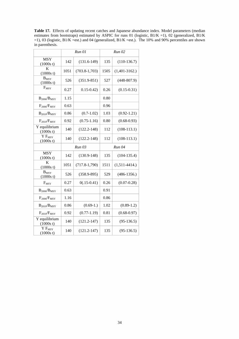
34

Table 17. Effects of updating recent catches and Japanese abundance index. Model parameters (median estimates from bootstraps) estimated by ASPIC for runs 01 (logistic, B1/K =1), 02 (generalized, B1/K =1), 03 (logistic, B1/K =est.) and 04 (generalized, B1/K =est.). The 10% and 90% percentiles are shown in parenthesis.

Run 01 Run 02

MSY (1000s t) 142 (131.6-149) 135 (110-136.7)

K (1000s t) 1051 (703.8-1,703) 1505 (1,401-3162.)

BMSY (1000s t) 526 (351.9-851) 527 (448-807.9)

FMSY 0.27 0.15-0.42) 0.26 (0.15-0.31)

B2006/BMSY 1.15 0.80

F2006/FMSY 0.63 0.96

B2010/BMSY 0.86 (0.7-1.02) 1.03 (0.92-1.21)

F2010/FMSY 0.92 (0.75-1.16) 0.80 (0.68-0.93) Y equilibrium

(1000s t) 140 (122.2-148) 112 (108-113.1)

Y FMSY (1000s t) 140 (122.2-148) 112 (108-113.1)

Run 03 Run 04

MSY (1000s t) 142 (130.9-148) 135 (104-135.4)

K (1000s t) 1051 (717.8-1,790) 1511 (1,511-4414.)

BMSY (1000s t) 526 (358.9-895) 529 (486-1356.)

FMSY 0.27 0(.15-0.41) 0.26 (0.07-0.28)

B2006/BMSY 0.63 0.91

F2006/FMSY 1.16 0.86

B2010/BMSY 0.86 (0.69-1.) 1.02 (0.89-1.2)


(1000s t) 140 (121.2-147) 135 (95-136.5)

Y FMSY (1000s t) 140 (121.2-147) 135 (95-136.5)

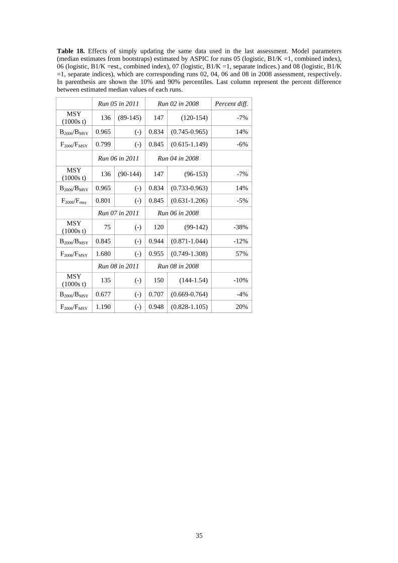
35

Table 18. Effects of simply updating the same data used in the last assessment. Model parameters (median estimates from bootstraps) estimated by ASPIC for runs 05 (logistic, B1/K =1, combined index), 06 (logistic, B1/K =est., combined index), 07 (logistic, B1/K =1, separate indices.) and 08 (logistic, B1/K =1, separate indices), which are corresponding runs 02, 04, 06 and 08 in 2008 assessment, respectively. In parenthesis are shown the 10% and 90% percentiles. Last column represent the percent difference between estimated median values of each runs.

Run 05 in 2011 Run 02 in 2008 Percent diff.

MSY (1000s t) 136 (89-145) 147 (120-154) -7%

B2006/BMSY 0.965 (-) 0.834 (0.745-0.965) 14%

F2006/FMSY 0.799 (-) 0.845 (0.615-1.149) -6%

Run 06 in 2011 Run 04 in 2008

MSY (1000s t) 136 (90-144) 147 (96-153) -7%

B2006/BMSY 0.965 (-) 0.834 (0.733-0.963) 14%

F2006/Fmsy 0.801 (-) 0.845 (0.631-1.206) -5%

Run 07 in 2011 Run 06 in 2008 MSY

(1000s t) 75 (-) 120 (99-142) -38%

B2006/BMSY 0.845 (-) 0.944 (0.871-1.044) -12%

F2006/FMSY 1.680 (-) 0.955 (0.749-1.308) 57%

Run 08 in 2011 Run 08 in 2008 MSY

(1000s t) 135 (-) 150 (144-1.54) -10%

B2006/BMSY 0.677 (-) 0.707 (0.669-0.764) -4%

F2006/FMSY 1.190 (-) 0.948 (0.828-1.105) 20%

36

Table 19. Effects of simply updating the same data used in the last assessment. Model parameters (median estimates from bootstraps) estimated by ASPIC for runs 05 (logistic, B1/K =1, combined index), 06 (logistic, B1/K =est., combined index), 07 (logistic, B1/K =1, separate indices.) and 08 (logistic, B1/K =1, separate indices). The 10% and 90% percentiles are shown in parentheses.

Run 05 in 2011 Run 06 in 2011

MSY (1000s t) 136 (89-145) 136 (89-144)

K (1000s t) 1,930 (1,140-6,070) 1,970 (1,240-6,120)

BMSY (1000s t) 967 (571-3,040) 983 (620-3,060)

FMSY 0.141 (0.030-0.246) 0.138 (0.029-0.226)

B2010/BMSY 1.108 (0.862-1.298) 1.104 (0.865-1.339)


(1000s t) 134 (130-142) 134 (125-141)

Y FMSY (1000s t) 111 (109-113) 111 (108-113)

Run 07 in 2011 Run 08 in 2011

MSY (1000s t) 75 (65-88)* 135 (125-142)*

K (1000s t) 584 (573-6,020)* 1,500 (542-1,070)*

BMSY (1000s t) 2,920 (2,870-3,010)* 749 (1,080-2,150)*

FMSY 0.026 0.180

B2010/BMSY 0.785 (0.685-0.906)* 0.795 (0.709-0.905)*

F2010/FMSY 1.821 (1.348-2.448)* 1.027 (0.880-1.210)* Y equilibrium

(1000s t) 71.4 129

Y FMSY (1000s t) 59.2 109

*These values were not derived from .bot file due to lack of output of these values. Therefore, these values were calculated from another output files (.det file) using simple percentile.

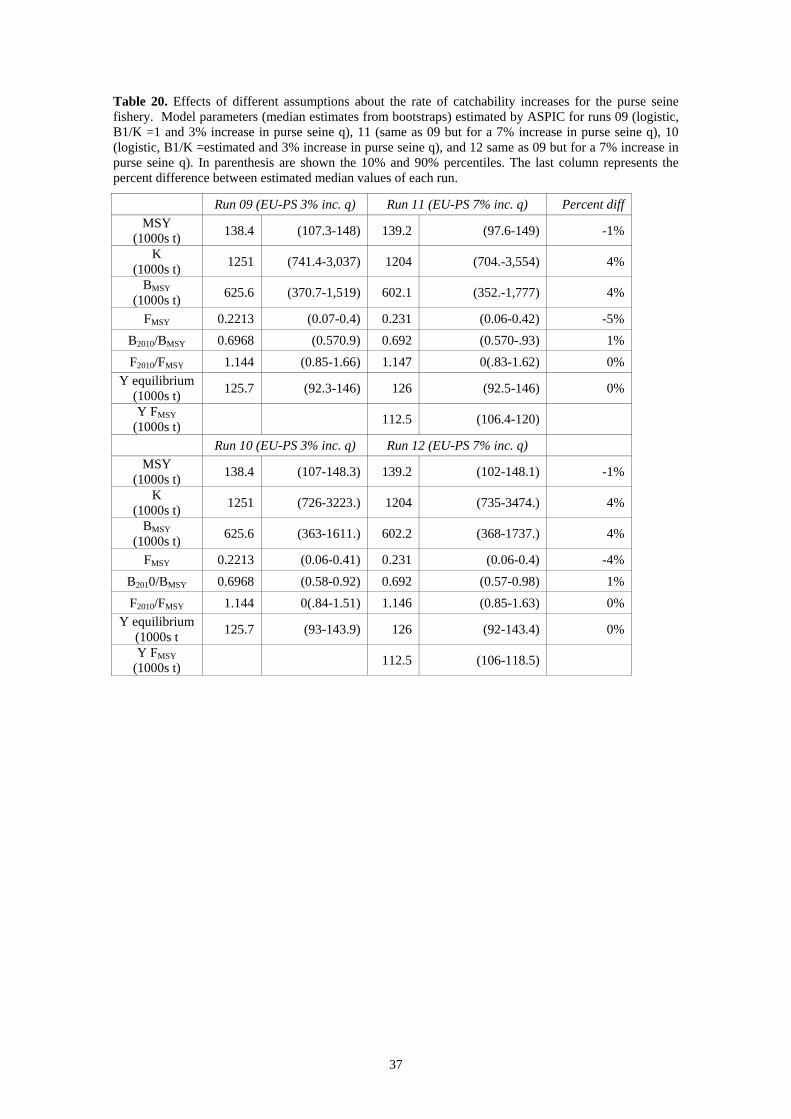
37

Table 20. Effects of different assumptions about the rate of catchability increases for the purse seine fishery. Model parameters (median estimates from bootstraps) estimated by ASPIC for runs 09 (logistic, B1/K =1 and 3% increase in purse seine q), 11 (same as 09 but for a 7% increase in purse seine q), 10 (logistic, B1/K =estimated and 3% increase in purse seine q), and 12 same as 09 but for a 7% increase in purse seine q). In parenthesis are shown the 10% and 90% percentiles. The last column represents the percent difference between estimated median values of each run.

Run 09 (EU-PS 3% inc. q) Run 11 (EU-PS 7% inc. q) Percent diff

MSY (1000s t) 138.4 (107.3-148) 139.2 (97.6-149) -1%

K (1000s t) 1251 (741.4-3,037) 1204 (704.-3,554) 4%

BMSY (1000s t) 625.6 (370.7-1,519) 602.1 (352.-1,777) 4%

FMSY 0.2213 (0.07-0.4) 0.231 (0.06-0.42) -5% B2010/BMSY 0.6968 (0.570.9) 0.692 (0.570-.93) 1% F2010/FMSY 1.144 (0.85-1.66) 1.147 0(.83-1.62) 0%

Y equilibrium (1000s t) 125.7 (92.3-146) 126 (92.5-146) 0%

Y FMSY (1000s t) 112.5 (106.4-120)

Run 10 (EU-PS 3% inc. q) Run 12 (EU-PS 7% inc. q) MSY

(1000s t) 138.4 (107-148.3) 139.2 (102-148.1) -1%

K (1000s t) 1251 (726-3223.) 1204 (735-3474.) 4%

BMSY (1000s t) 625.6 (363-1611.) 602.2 (368-1737.) 4%

FMSY 0.2213 (0.06-0.41) 0.231 (0.06-0.4) -4% B2010/BMSY 0.6968 (0.58-0.92) 0.692 (0.57-0.98) 1% F2010/FMSY 1.144 0(.84-1.51) 1.146 (0.85-1.63) 0%

Y equilibrium (1000s t 125.7 (93-143.9) 126 (92-143.4) 0%

Y FMSY (1000s t) 112.5 (106-118.5)

38

Table 21. Effects of revision of Ghana catch. Model parameters (median estimates from bootstraps) estimated by ASPIC for runs 11 (Task I catch) and 14 (including estimated revisions for Ghana). In parenthesis are shown the 10% and 90% percentiles. The last column represents the percent difference between estimated median values of run 14 and run 11.

Run 11 Run 14 Percent diff.

MSY (1000s t) 139 (97.6-149) 144 (113-151.6) -3%

K (1000s t) 1204 (704.-3,554) 975 (584-2806.) 19%

BMSY (1000s t) 602 (352.-1,777) 487 (292-1403.) 19%

FMSY 0.23 (0.06-0.42) 0.30 (0.08-0.52) -28%

B2010/BMSY 0.69 (0.57-0.93) 0.66 (0.54-0.87) 5%

F2010/FMSY 1.15 (0.83-1.62) 1.34 (0.96-1.7) -17%

Y equilibrium (1000s t) 126 (92.5-146) 127 (104-148.) -1%

Y FMSY (1000s t) 113 (106.4-120) 127 (122-135.1) -13%

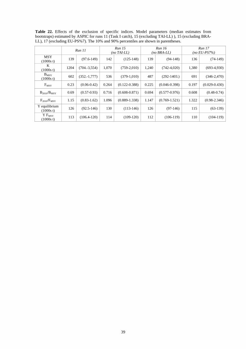
39

Table 22. Effects of the exclusion of specific indices. Model parameters (median estimates from bootstraps) estimated by ASPIC for runs 11 (Task I catch), 15 (excluding TAI-LL) ), 15 (excluding BRA-LL), 17 (excluding EU-PS%7). The 10% and 90% percentiles are shown in parentheses.

Run 11 Run 15

(no TAI-LL) Run 16

(no BRA-LL) Run 17

(no EU-PS7%) MSY

(1000s t) 139 (97.6-149) 142 (125-148) 139 (94-148) 136 (74-149)

K (1000s t) 1204 (704.-3,554) 1,070 (759-2,010) 1,240 (742-4,020) 1,380 (693-4,930)

BMSY (1000s t) 602 (352.-1,777) 536 (379-1,010) 487 (292-1403.) 691 (346-2,470)

FMSY 0.23 (0.06-0.42) 0.264 (0.122-0.388) 0.225 (0.046-0.398) 0.197 (0.029-0.430)

B2010/BMSY 0.69 (0.57-0.93) 0.716 (0.608-0.871) 0.694 (0.577-0.976) 0.608 (0.48-0.74)

F2010/FMSY 1.15 (0.83-1.62) 1.096 (0.889-1.338) 1.147 (0.769-1.521) 1.322 (0.98-2.346) Y equilibrium

(1000s t) 126 (92.5-146) 130 (113-146) 126 (97-146) 115 (63-139)

Y FMSY (1000s t) 113 (106.4-120) 114 (109-120) 112 (106-119) 110 (104-119)

40

Table 23. Maximum posterior estimates for PROCEAN parameters and fishery-derived indicators. CAI = Combined abundance index. * indicates that the parameters were fixed.

m r B0/K K MSY F/FMSY B/BMSY

Base case runs

CAI unweighted 2.3 0.81 0.9* 602224 145416 1.18 0.65

CAI weighted by area 1.85 0.76 0.9* 844301 143494 1.16 0.68

Initial biomass 1.93 0.84 0.8* 737754 146441 1.16 0.68

Shape parameter 1.5* 1.05 0.9* 896992 139065 1.13 0.74

Data inputs in the CAI

Index without TAI 1.85* 0.64 0.9* 1020000 145052 1.08 0.68

Index without BRZ 1.85* 0.57 0.9* 1150000 145848 1.14 0.68

Index without EUR-PS 1.85* 0.5 0.9* 1230000 137451 1.24 0.62

Multiple indices

6 CPUE indices 1.85* 0.51 0.9* 1310000 148245 0.89 0.78

5 CPUE indices (excl. TAI-LL 1968-2010)

1.85* 0.52 0.9* 1320000 148000 0.89 0.78

4 CPUE indices (excl. TAI-LL and BRA-LL)

1.26 0.67 0.9* 2350000 134237 0.9 0.86

41

Table 24. VPA estimates of management benchmarks and reference points.

BASE RUN 1 BASE RUN 2MEASURE LOWER 80% CI MEDIAN UPPER 80% CI Deterministic MEASURE LOWER 80% CI MEDIAN UPPER 80% CI Deterministic

F at MSY 0.827 1.115 1.425 1.448 F at MSY 0.771 0.823 0.880 0.874MSY 129,904 135,518 141,568 140,880 MSY 130,326 136,842 143,451 141,066 Y/R at MSY 2.228 2.324 2.409 2.412 Y/R at MSY 2.012 2.101 2.174 2.172S/R at MSY 2.310 2.456 2.577 2.551 S/R at MSY 1.975 2.045 2.104 2.056SPR AT MSY 0.222 0.237 0.248 0.246 SPR AT MSY 0.190 0.197 0.203 0.198SSB AT MSY 135,529 143,591 150,429 148,986 SSB AT MSY 128,673 133,555 138,176 133,586 F at max. Y/R 0.827 1.115 1.425 1.448 F at max. Y/R 0.771 0.823 0.880 0.874Y/R maximum 2.228 2.324 2.409 2.412 Y/R maximum 2.012 2.101 2.174 2.172S/R at Fmax 2.310 2.456 2.577 2.551 S/R at Fmax 1.975 2.045 2.104 2.056SPR at Fmax 0.222 0.237 0.248 0.246 SPR at Fmax 0.190 0.197 0.203 0.198SSB at Fmax 135,529 143,591 150,429 148,986 SSB at Fmax 128,673 133,555 138,176 133,586 F 0.1 0.504 0.626 0.738 0.745 F 0.1 0.511 0.541 0.572 0.568Y/R at F0.1 2.085 2.150 2.200 2.202 Y/R at F0.1 1.916 1.994 2.059 2.059S/R at F0.1 3.859 4.168 4.436 4.428 S/R at F0.1 3.278 3.384 3.487 3.416SPR at F0.1 0.372 0.401 0.427 0.426 SPR at F0.1 0.316 0.326 0.336 0.329SSB at F0.1 226,518 243,532 258,609 258,589 SSB at F0.1 213,472 221,025 228,657 221,927

BASE RUN 3 BASE RUN 4MEASURE LOWER 80% CI MEDIAN UPPER 80% CI Deterministic MEASURE LOWER 80% CI MEDIAN UPPER 80% CI Deterministic

F at MSY 0.774 0.897 1.083 1.181 F at MSY 0.755 0.801 0.934 0.819MSY 125,263 129,884 134,989 135,917 MSY 121,278 126,628 131,870 130,809 Y/R at MSY 2.191 2.260 2.333 2.359 Y/R at MSY 2.113 2.197 2.280 2.266S/R at MSY 2.255 2.347 2.441 2.448 S/R at MSY 2.141 2.259 2.378 2.283SPR AT MSY 0.217 0.226 0.235 0.236 SPR AT MSY 0.206 0.218 0.229 0.220SSB AT MSY 129,733 135,036 140,234 141,047 SSB AT MSY 123,875 129,918 136,714 131,815 F at max. Y/R 0.774 0.897 1.083 1.181 F at max. Y/R 0.755 0.801 0.934 0.819Y/R maximum 2.191 2.260 2.333 2.359 Y/R maximum 2.113 2.197 2.280 2.266S/R at Fmax 2.255 2.347 2.441 2.448 S/R at Fmax 2.141 2.259 2.378 2.283SPR at Fmax 0.217 0.226 0.235 0.236 SPR at Fmax 0.206 0.218 0.229 0.220SSB at Fmax 129,733 135,036 140,234 141,047 SSB at Fmax 123,875 129,918 136,714 131,815 F 0.1 0.476 0.530 0.613 0.650 F 0.1 0.473 0.499 0.549 0.493Y/R at F0.1 2.058 2.111 2.164 2.177 Y/R at F0.1 1.997 2.066 2.127 2.122S/R at F0.1 3.751 3.941 4.122 4.191 S/R at F0.1 3.548 3.752 3.986 3.833SPR at F0.1 0.361 0.380 0.397 0.404 SPR at F0.1 0.342 0.361 0.384 0.369SSB at F0.1 215,614 226,339 237,522 241,450 SSB at F0.1 204,911 215,775 229,975 221,249

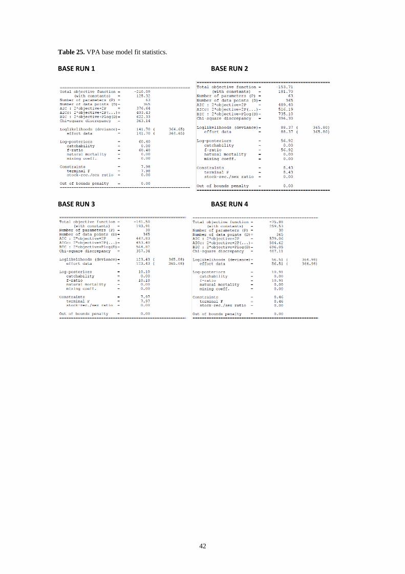
42

Table 25. VPA base model fit statistics.

BASE RUN 1 BASE RUN 2

BASE RUN 3 BASE RUN 4

43

Table 26. Management benchmarks and references developed from the ASPIC/VPA joint distribution.

Relative Biomass (SSB2010/SSBMSY for VPA, B2011/BMSY for ASPIC)

Method Median 10th percentile 90th percentile Production model

(ASPIC) 0.6946 0.5701 0.9243

Age-Structured model (VPA) 0.5248 0.4253 0.6722

Combined distribution (ASPIC and VPA) 0.6123 0.4551 0.8451

Relative Fishing Mortality (Fcurrent/FMSY for VPA, F2010/FMSY for ASPIC)

Method Median 10th percentile 90th percentile

Production model (ASPIC) 1.0861 0.7466 1.6255

Age-Structured model (VPA) 1.3222 1.1462 1.5056

Combined distribution (ASPIC and VPA) 1.2540 0.8545 1.5329

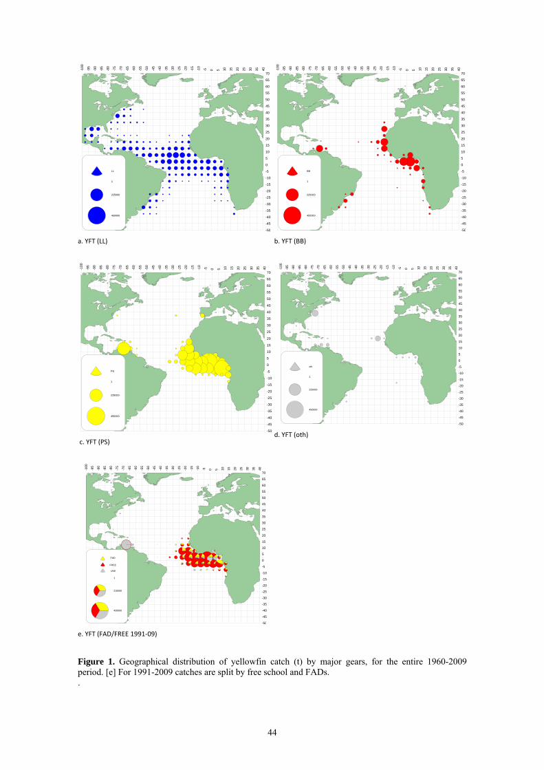
44

a. YFT (LL)

b. YFT (BB)

c. YFT (PS)

d. YFT (oth)

e. YFT (FAD/FREE 1991‐09)

Figure 1. Geographical distribution of yellowfin catch (t) by major gears, for the entire 1960-2009 period. [e] For 1991-2009 catches are split by free school and FADs. .

-100

-95

-90

-85

-80

-75

-70

-65

-60

-55

-50

-45

-40

-35

-30

-25

-20

-15

-10

-5 0 5 10 15 20 25 30 35 40

-50

-45

-40

-35

-30

-25

-20

-15

-10

-5

0

5

10

15

20

25

30

35

40

45

50

55

60

65

70

LL

1

225000

450000

-100

-95

-90

-85

-80

-75

-70

-65

-60

-55

-50

-45

-40

-35

-30

-25

-20

-15

-10

-5 0 5 10 15 20 25 30 35 40

-50

-45

-40

-35

-30

-25

-20

-15

-10

-5

0

5

10

15

20

25

30

35

40

45

50

55

60

65

70

BB

1

225000

450000

-10

0

-95

-90

-85

-80

-75

-70

-65

-60

-55

-50

-45

-40

-35

-30

-25

-20

-15

-10

-5 0 5 10 15 20 25 30 35 40

-50

-45

-40

-35

-30

-25

-20

-15

-10

-5

0

5

10

15

20

25

30

35

40

45

50

55

60

65

70

PS

1

225000

450000

-100

-95

-90

-85

-80

-75

-70

-65

-60

-55

-50

-45

-40

-35

-30

-25

-20

-15

-10

-5 0 5 10 15 20 25 30 35 40

-50

-45

-40

-35

-30

-25

-20

-15

-10

-5

0

5

10

15

20

25

30

35

40

45

50

55

60

65

70

oth

1

225000

450000

-100

-95

-90

-85

-80

-75

-70

-65

-60

-55

-50

-45

-40

-35

-30

-25

-20

-15

-10

-5 0 5 10 15 20 25 30 35 40

-50

-45

-40

-35

-30

-25

-20

-15

-10

-5

0

5

10

15

20

25

30

35

40

45

50

55

60

65

70

FAD

FREE

UNK

1

210000

420000

45

a. YFT(1960‐69) b. YFT(1970‐79)

c. YFT(1980‐89) d. YFT(1990‐99)

e. YFT (2000‐09)

Figure 2. Geographical distribution of yellowfin catch by major gear and decade.

46

Figure 3. Atlantic yellowfin tuna catch by area.

Figure 4. Atlantic yellowfin tuna catch by gear.

0

50

100

150

200

250

1950

1953

1956

1959

1962

1965

1968

1971

1974

1977

1980

1983

1986

1989

1992

1995

1998

2001

2004

2007

2010

Thousand tons

ATW

ATE

0

50

100

150

200

250

1950

1953

1956

1959

1962

1965

1968

1971

1974

1977

1980

1983

1986

1989

1992

1995

1998

2001

2004

2007

2010

Thousand tons Others

LL

BB

PS

47

Figure 5. Catch by gear east.

Figure 6. Catch by gear west.

0

20000

40000

60000

80000

100000

120000

140000

160000

180000

1950

1953

1956

1959

1962

1965

1968

1971

1974

1977

1980

1983

1986

1989

1992

1995

1998

2001

2004

2007

2010

ATE others

ATE LL

ATE PS

ATE BB

0

10000

20000

30000

40000

50000

60000

1950

1953

1956

1959

1962

1965

1968

1971

1974

1977

1980

1983

1986

1989

1992

1995

1998

2001

2004

2007

2010

ATW others

ATW LL

ATW PS

ATW BB

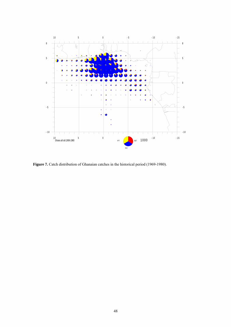
48

Figure 7. Catch distribution of Ghanaian catches in the historical period (1969-1980).

- 10

- 5

0

5

8

- 1 5- 1 0- 5051 0

- 1 5- 1 0- 5051 0

- 1 0

- 5

0

5

8

Ghana all old 1969-1980 1000YFT BET

SKJ

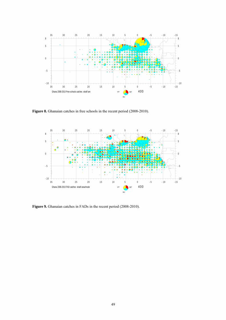
49

Figure 8. Ghanaian catches in free schools in the recent period (2008-2010).

Figure 9. Ghanaian catches in FADs in the recent period (2008-2010).

- 1 0

- 5

0

5

8- 1 5- 1 0- 5051 01 52 02 53 03 5

- 1 5- 1 0- 5051 01 52 02 53 03 5- 1 0

- 5

0

5

8

Ghana 2008-2010 Free schools catches stratif are 4 0 0YFT BET

SKJ

- 1 0

- 5

0

5

8- 1 5- 1 0- 5051 01 52 02 53 03 5

- 1 5- 1 0- 5051 01 52 02 53 03 5- 1 0

- 5

0

5

8

Ghana 2008-2010 FAD catches stratif area/mode 4 0 0YFT BET

SKJ

50

Figure 10. European and associated fishery catch on FADs in 2009.

Figure 11. Carrying capacity of the surface fleets in the East Atlantic for the period 1972-2010.

- 15

- 10

0

10- 15- 10010203040

- 15- 10010203040- 15

- 10

0

10

EU PS FAD catches 2009 1000YFT BET

SKJ

0

10

20

30

40

50

60

70

80

0

10

20

30

40

50

60

70

80

1970 1974 1978 1982 1986 1990 1994 1998 2002 2006 2010

Nb

bo

ats

Car

ryin

g c

apac

ity

(10

00 t

)

Years

East Atlantic

TOTAL BB TOTAL PS Nb EU+NEI PS

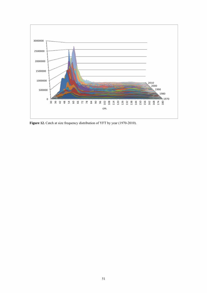
51

Figure 12. Catch at size frequency distribution of YFT by year (1970-2010).

1970

1980

19902000

2010

0

500000

1000000

1500000

2000000

2500000

3000000

30 36 42 48 54 60 66 72 78 84 90 96 102

108

114

120

126

132

138

144

150

156

162

168

174

180

cm.

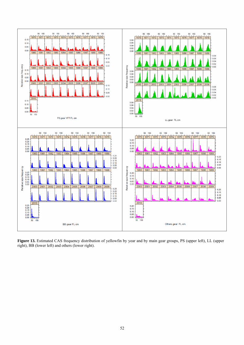
52

Figure 13. Estimated CAS frequency distribution of yellowfin by year and by main gear groups, PS (upper left), LL (upper right), BB (lower left) and others (lower right).

53

Figure 14. Catch at age of yellowfin tuna 1970-2010 estimated as input for the age structure model(s).

0

1

2

3

4

5

Age

1965 1970 1975 1980 1985 1990 1995 2000 2005 2010 2015

Year

Circle Size

CAA yellowfin tuna slicing Gascuel growth model (age 5+)

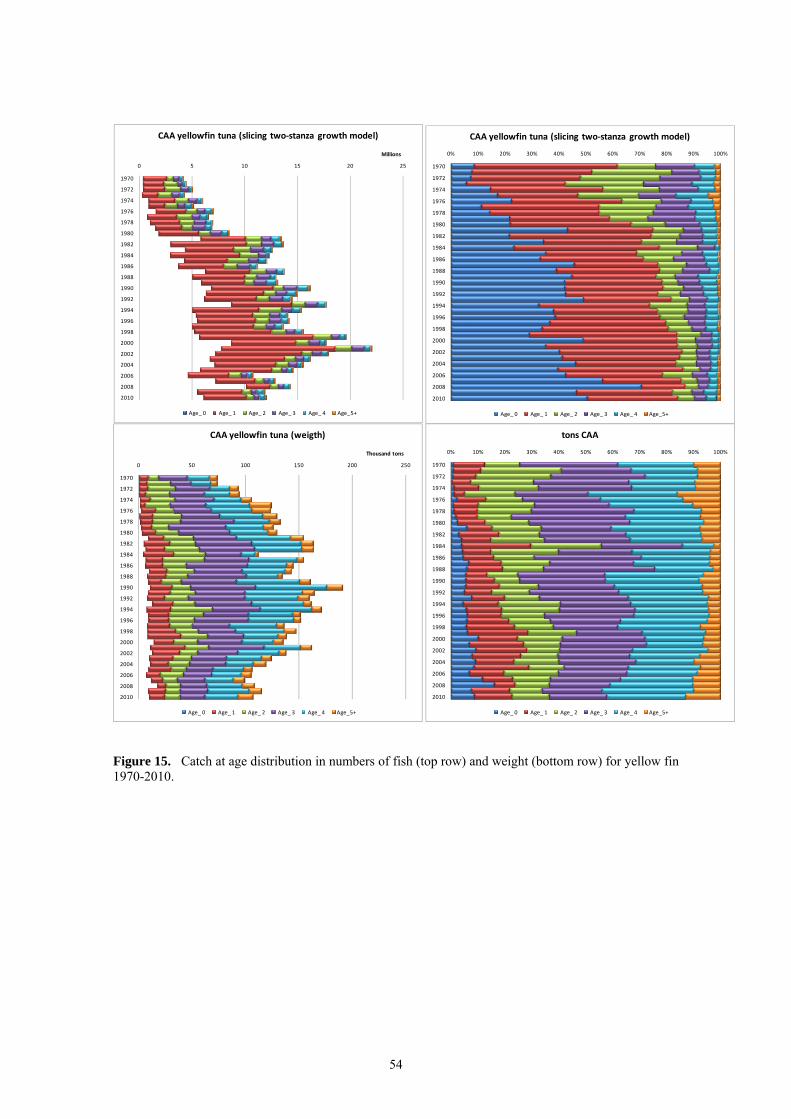
54

Figure 15. Catch at age distribution in numbers of fish (top row) and weight (bottom row) for yellow fin 1970-2010.

0 5 10 15 20 25

1970

1972

1974

1976

1978

1980

1982

1984

1986

1988

1990

1992

1994

1996

1998

2000

2002

2004

2006

2008

2010

Millions

CAA yellowfin tuna (slicing two‐stanza growth model)

Age_ 0 Age_ 1 Age_ 2 Age_ 3 Age_ 4 Age_5+

0% 10% 20% 30% 40% 50% 60% 70% 80% 90% 100%

1970

1972

1974

1976

1978

1980

1982

1984

1986

1988

1990

1992

1994

1996

1998

2000

2002

2004

2006

2008

2010

CAA yellowfin tuna (slicing two‐stanza growth model)


0 50 100 150 200 250

1970

1972

1974

1976

1978

1980

1982

1984

1986

1988

1990

1992

1994

1996

1998

2000

2002

2004

2006

2008

2010

Thousand tons

CAA yellowfin tuna (weigth)


0% 10% 20% 30% 40% 50% 60% 70% 80% 90% 100%

1970

1972

1974

1976

1978

1980

1982

1984

1986

1988

1990

1992

1994

1996

1998

2000

2002

2004

2006

2008

2010

tons CAA


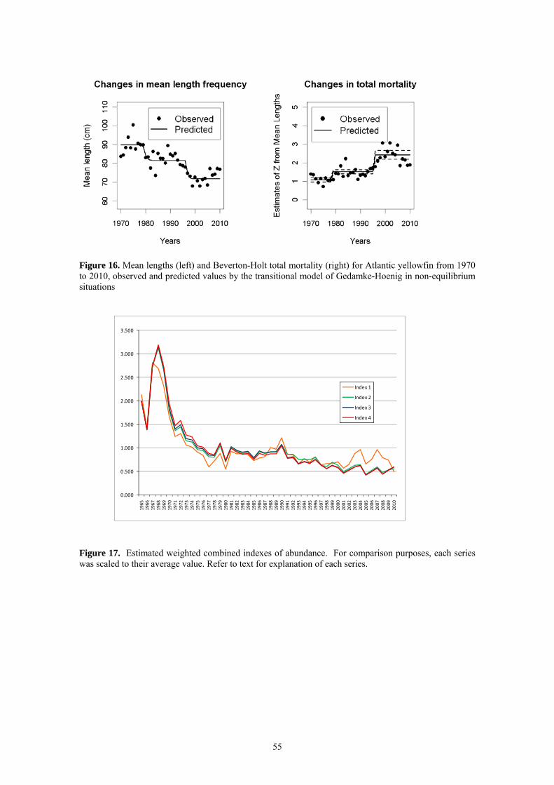
55

Figure 16. Mean lengths (left) and Beverton-Holt total mortality (right) for Atlantic yellowfin from 1970 to 2010, observed and predicted values by the transitional model of Gedamke-Hoenig in non-equilibrium situations

Figure 17. Estimated weighted combined indexes of abundance. For comparison purposes, each series was scaled to their average value. Refer to text for explanation of each series.

0.000

0.500

1.000

1.500

2.000

2.500

3.000

3.500

1965

1966

1967

1968

1969

1970

1971

1972

1973

1974

1975

1976

1977

1978

1979

1980

1981

1982

1983

1984

1985

1986

1987

1988

1989

1990

1991

1992

1993

1994

1995

1996

1997

1998

1999

2000

2001

2002

2003

2004

2005

2006

2007

2008

2009

2010

Index 1

Index 2

Index 3

Index 4

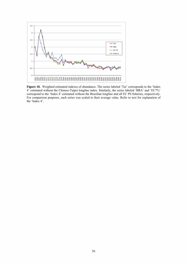
56

Figure 18. Weighted estimated indexes of abundance. The series labeled ‘Tai’ corresponds to the ‘Index 4’ estimated without the Chinese-Taipei longline index. Similarly, the series labeled ‘BRA’ and ‘EC7%’ correspond to the ‘Index 4’ estimated without the Brazilian longline and all EC PS fisheries, respectively. For comparison purposes, each series was scaled to their average value. Refer to text for explanation of the ‘Index 4’.

0

0.5

1

1.5

2

2.5

3

3.5

1965

1966

1967

1968

1969

1970

1971

1972

1973

1974

1975

1976

1977

1978

1979

1980

1981

1982

1983

1984

1985

1986

1987

1988

1989

1990

1991

1992

1993

1994

1995

1996

1997

1998

1999

2000

2001

2002

2003

2004

2005

2006

2007

2008

2009

2010

TAI

BRA

EC 7%

Index 4

57

Figure 19. Effects of simply updating the same data used in the last assessment. Biomass ratios and fishing mortality ratios by year from ASPIC for runs 9 (3 % increase in catchability for purse seine) and 11 (7% increase in catchability for purse seine).

0

1

2

0 1 2

F/Fm

sy

B/Bmsy

Effect of simply update catch and CPUE index (combined)

B1/K fix, logstic model

run02_2008 run05_2011

2006

0

1

2

0 1 2

F/Fm

syB/Bmsy

Effect of simply update catch and CPUE index (combined)

B1/K estimate, logstic model

run04_2008 run06_2011

2006

0

1

2

0 1 2

F/Fm

sy

B/Bmsy

Effect of simply update catch and CPUE index (separate, no area weight)


run06_2008 run06_2011

2006

0

1

2

0 1 2

F/Fm

sy

B/Bmsy

Effect of simply update catch and CPUE index (separate, area weight)


run08_2008 run08_2011

2006

58

Figure 20. Effects of assumption on percent increase catchability in purse seine fleet . Biomass ratios and fishing mortality ratios by year from ASPIC for runs 9 (3 % increase in catchability for purse seine) and 11 (7% increase in catchability for purse seine). Left panel (whole time series 1950 to 2010), right panel (recent years 2006 to 2010).

Figure 21. Results of bootstrap examination for Run 09 to Run 12.

0

1

2

0 1 2

F/Fm

sy

B/Bmsy

comparison 3 % and 7% (run09 and run11)

F/Fmsy_run09_2011 F/Fmsy_run10_2011

2010

0

1

2

0 1 2

F/Fm

sy

B/Bmsy

comparison 3 % and 7% (run09 and run11)recent years (2006 to 2010)

F/Fmsy_run09_2011 F/Fmsy_run10_2011

2010

2006

0

1

2

3

0 1 2

F/Fm

sy

B/Bmsy

Run10, B1/K estimate, logistic, new combined PS 3% inc. q

0

1

2

3

0 1 2

F/Fm

sy

B/Bmsy

Run09, B1/K fix, logistic, new combined PS 3% inc. q

0

1

2

3

0 1 2

F/Fm

sy

B/Bmsy

Run11, B1/K fix, logistic, new combined PS 7% inc. q

0

1

2

3

0 1 2

F/Fm

sy

B/Bmsy

Run12, B1/K festimate, logistic, new combined PS 7% inc. q

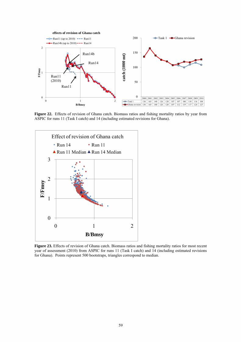
59

Figure 22. Effects of revision of Ghana catch. Biomass ratios and fishing mortality ratios by year from ASPIC for runs 11 (Task I catch) and 14 (including estimated revisions for Ghana).

Figure 23. Effects of revision of Ghana catch. Biomass ratios and fishing mortality ratios for most recent year of assessment (2010) from ASPIC for runs 11 (Task I catch) and 14 (including estimated revisions for Ghana). Points represent 500 bootstraps, triangles correspond to median.

0

1

2

0 1 2

F/Fm

sy

B/Bmsy

effects of revision of Ghana catch

Run11 (up to 2010) Run11

Run14b (up to 2010) Run14

Run11

Run14

Run14b

Run11 (2010)

2000 2001 2002 2003 2004 2005 2006 2007 2008 2009 2010

Task 1 136 165 140 126 120 107 107 100 110 116 108

Ghana revision 136 165 140 126 120 107 112 119 117 124 127

0

50

100

150

200

catc

h (1

000

mt)

Task 1 Ghana revision

0

1

2

3

0 1 2

F/Fm

sy

B/Bmsy

Effect of revision of Ghana catch

Run 14 Run 11

Run 11 Median Run 14 Median

60

Figure 24. Effects of excluding of specific fleets when processing a combined index. Biomass ratios and fishing mortality ratios by year from ASPIC for excluding Chinese Taipei-LL (run 15), Brazilian-LL (run 16) and EU-PS 7% inc. q (run 17).

0

1

2

0 1 2

F/Fm

sy

B/Bmsy

Comparison Run11 and excluding TWN-LL, BR-LL and EU-PS inc. q 7%

all_run11 TWN (Run15)

BRLL (Run16) EU-PS inc. q 7%

EU‐PS 7% at 2010

run11, TWN‐LL and BR‐LL at 2010

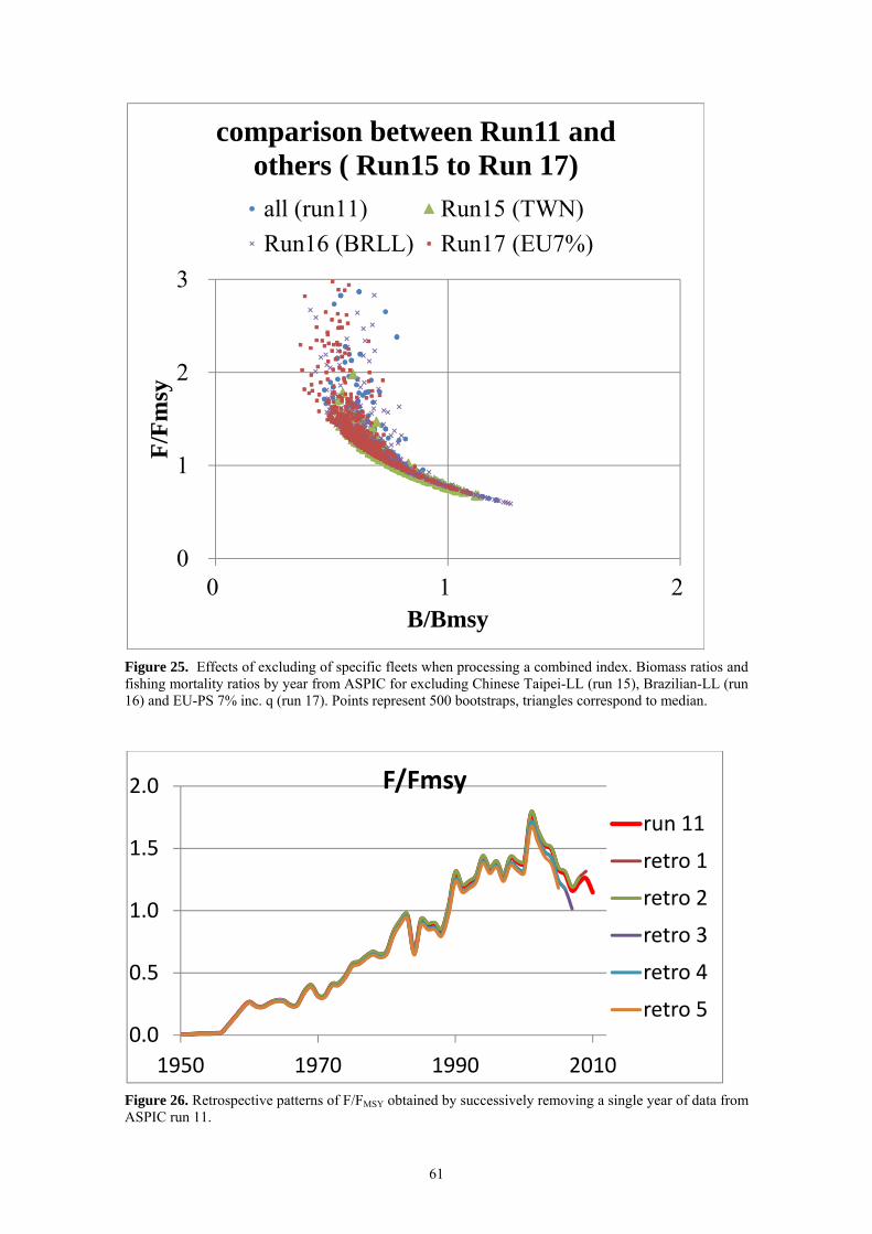
61

Figure 25. Effects of excluding of specific fleets when processing a combined index. Biomass ratios and fishing mortality ratios by year from ASPIC for excluding Chinese Taipei-LL (run 15), Brazilian-LL (run 16) and EU-PS 7% inc. q (run 17). Points represent 500 bootstraps, triangles correspond to median.

Figure 26. Retrospective patterns of F/FMSY obtained by successively removing a single year of data from ASPIC run 11.

0

1

2

3

0 1 2

F/Fm

sy

B/Bmsy

comparison between Run11 and others ( Run15 to Run 17)all (run11) Run15 (TWN)

Run16 (BRLL) Run17 (EU7%)

0.0

0.5

1.0

1.5

2.0

1950 1970 1990 2010

F/Fmsy

run 11

retro 1

retro 2

retro 3

retro 4

retro 5

62

Figure 27. Retrospective patterns of B/BMSY obtained by successively removing a single year of data from ASPIC run 11.

Figure 28. Retrospective view of r and K obtained by progressively eliminating successive years for ASPIC run 11 (combined CPUE with 7% increase in q on EU-PS)

0.40.60.81.01.21.41.61.82.0

1950 1970 1990 2010

B/Bmsy

run 11

retro 1

retro 2

retro 3

retro 4

retro 5

0.00

0.10

0.20

0.30

0.40

0.50

0.60

0.70

600

700

800

900

1,000

1,100

1,200

1,300

1,400

retro5 retro4 retro3 retro2 retro1 Run11

MT

Thousands

ASPIC, run 11 (comb CPUE), retrospective view of r and K

K

r

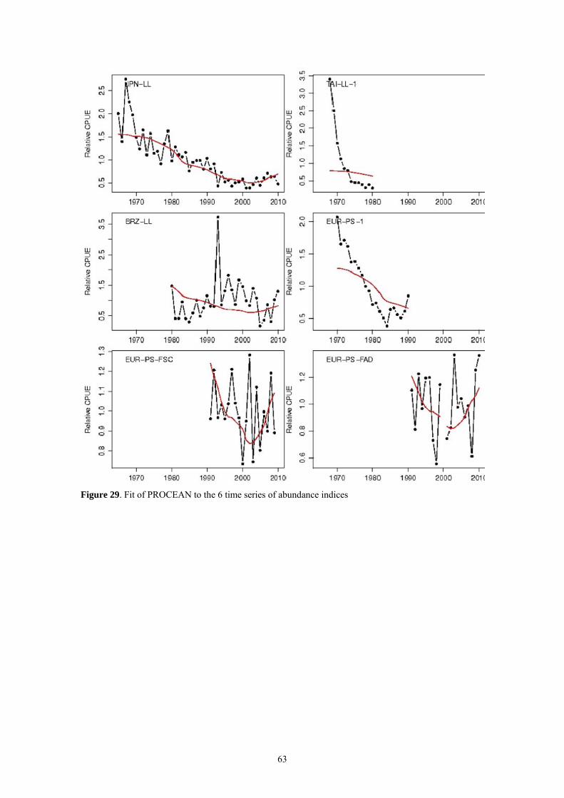
63

Figure 29. Fit of PROCEAN to the 6 time series of abundance indices

64

Figure 30. Phase diagram (“Kobe plot”) representing the evolution of the annual fishing mortality relative to the fishing mortality at MSY (F/FMSY) as a function of the annual biomass relative to the biomass at MSY (B/BMSY). PROCEAN fits to the combined abundance index weighted by area (upper figure) and the abundance indices for the JPN-LL, TAI-LL (1968-1980), BRZ-LL, EUR-PS (1979-1990), EUR-PS-FSC(1991-2010) and EUR-PS-FAD (1991-2010) (lower figure).

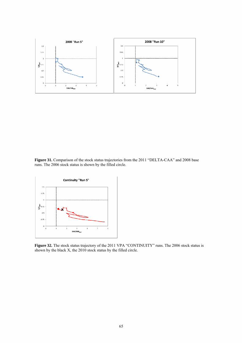
65

Figure 31. Comparison of the stock status trajectories from the 2011 “DELTA-CAA” and 2008 base runs. The 2006 stock status is shown by the filled circle.

Figure 32. The stock status trajectory of the 2011 VPA “CONTINUITY” runs. The 2006 stock status is shown by the black X, the 2010 stock status by the filled circle.

66

Figure 33. Results of VPA Base Run 1: annual trends in recruits (Age 0), total biomass, apical fishing mortality with regard to FMSY, spawning stock biomass with regard to SSBMSY and yield (t).

0

100000

200000

300000

400000

500000

600000

700000

1970 1980 1990 2000 2010

Total Biomass (m

t)

YEAR

Total Biomass (mt)

Lower 80% CI

Median

Upper 80% CI

0

10000000

20000000

30000000

40000000

50000000

60000000

70000000

80000000

90000000

1970 1980 1990 2000 2010

Recruits

YEAR

Recruits

Lower 80% CI

Median

Upper 80% CI

0

0.5

1

1.5

2

2.5

3

1970 1980 1990 2000 2010

Fishing Mortality

YEAR

Fishing Mortality

Lower 80% CI

Median

Upper 80% CI

Fmsy

0

50000

100000

150000

200000

250000

300000

350000

1970 1980 1990 2000 2010

Spaw

ning Stock Biomass (m

t)YEAR

Spawning Stock Biomass (mt)

Lower 80% CI

Median

Upper 80% CI

SSBmsy

0

50000

100000

150000

200000

250000

1970 1980 1990 2000 2010

Yield (mt)

YEAR

Yield (mt)

Lower 80% CI

Median

Upper 80% CI

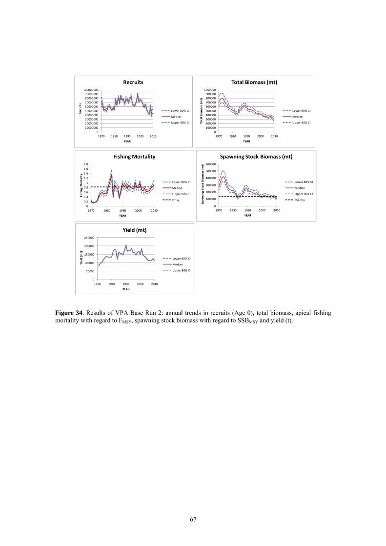
67


0100000200000300000400000500000600000700000800000900000

1000000

1970 1980 1990 2000 2010

Total Biomass (m

t)

YEAR

Total Biomass (mt)

Lower 80% CI

Median

Upper 80% CI

0100000002000000030000000400000005000000060000000700000008000000090000000

100000000

1970 1980 1990 2000 2010

Recruits

YEAR

Recruits

Lower 80% CI

Median

Upper 80% CI

0

0.2

0.4

0.6

0.8

1

1.2

1.4

1.6

1.8

1970 1980 1990 2000 2010

Fishing Mortality

YEAR

Fishing Mortality

Lower 80% CI

Median

Upper 80% CI

Fmsy

0

100000

200000

300000

400000

500000

600000

1970 1980 1990 2000 2010

Spaw


t)

YEAR


Lower 80% CI

Median

Upper 80% CI

SSBmsy

0

50000

100000

150000

200000

250000

1970 1980 1990 2000 2010

Yield (mt)

YEAR

Yield (mt)

Lower 80% CI

Median

Upper 80% CI

68


050000

100000150000200000250000300000350000400000450000500000

1970 1980 1990 2000 2010

Total Biomass (m

t)

YEAR

Total Biomass (mt)

Lower 80% CI

Median

Upper 80% CI

0

10000000

20000000

30000000

40000000

50000000

60000000

70000000

80000000

90000000

1970 1980 1990 2000 2010

Recruits

YEAR

Recruits

Lower 80% CI

Median

Upper 80% CI

0

0.5

1

1.5

2

2.5

1970 1980 1990 2000 2010

Fishing Mortality

YEAR

Fishing Mortality

Lower 80% CI

Median

Upper 80% CI

Fmsy

0

20000

40000

60000

80000

100000

120000

140000

160000

1970 1980 1990 2000 2010

Spaw


t)

YEAR


Lower 80% CI

Median

Upper 80% CI

SSBmsy

0

50000

100000

150000

200000

250000

1970 1980 1990 2000 2010

Yield (mt)

YEAR

Yield (mt)

Lower 80% CI

Median

Upper 80% CI

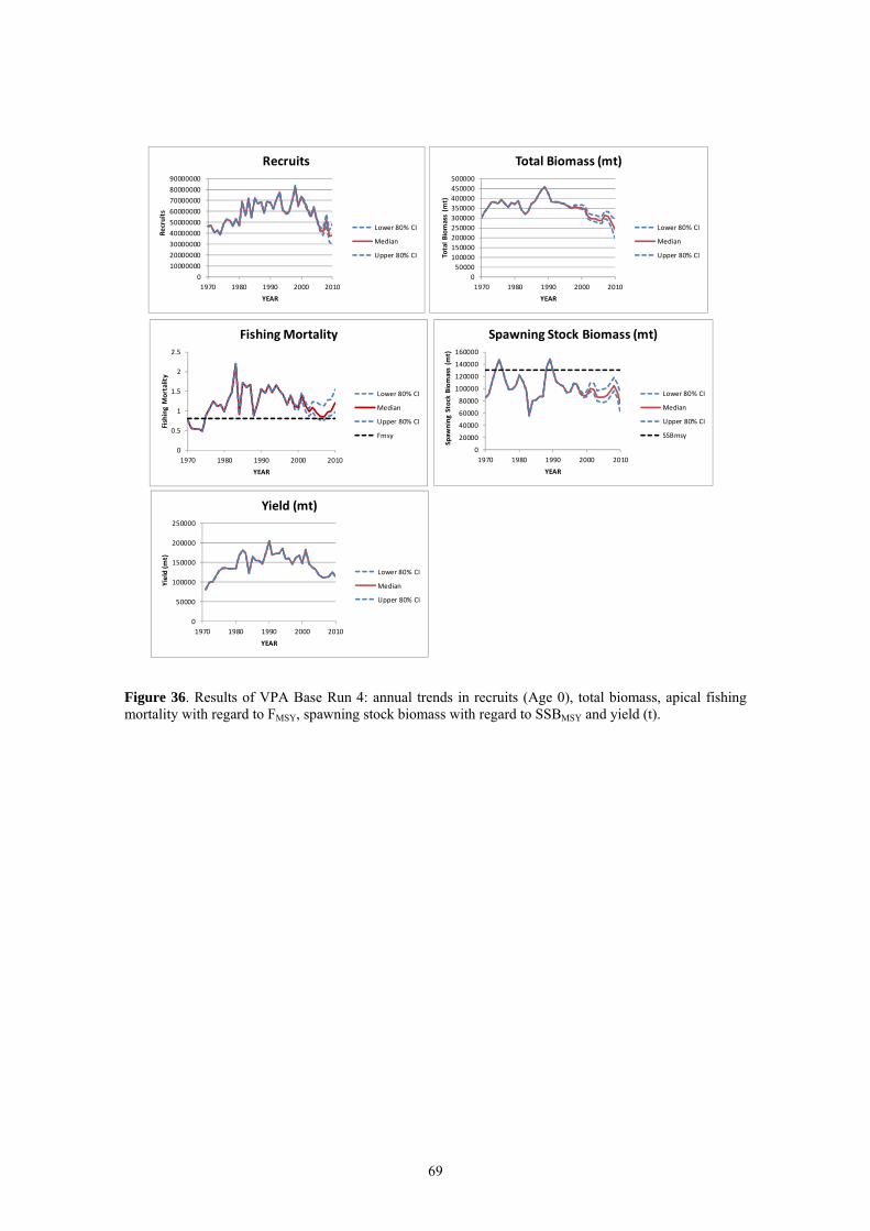
69


050000

100000150000200000250000300000350000400000450000500000

1970 1980 1990 2000 2010

Total Biomass (m

t)

YEAR

Total Biomass (mt)

Lower 80% CI

Median

Upper 80% CI

0

10000000

20000000

30000000

40000000

50000000

60000000

70000000

80000000

90000000

1970 1980 1990 2000 2010

Recruits

YEAR

Recruits

Lower 80% CI

Median

Upper 80% CI

0

0.5

1

1.5

2

2.5

1970 1980 1990 2000 2010

Fishing Mortality

YEAR

Fishing Mortality

Lower 80% CI

Median

Upper 80% CI

Fmsy

0

20000

40000

60000

80000

100000

120000

140000

160000

1970 1980 1990 2000 2010

Spaw


t)

YEAR


Lower 80% CI

Median

Upper 80% CI

SSBmsy

0

50000

100000

150000

200000

250000

1970 1980 1990 2000 2010

Yield (mt)

YEAR

Yield (mt)

Lower 80% CI

Median

Upper 80% CI

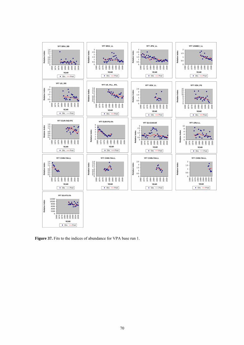
70

Figure 37. Fits to the indices of abundance for VPA base run 1.

00.20.40.60.8

11.21.41.6

19

69

19

74

19

79

19

84

19

89

19

94

19

99

20

04

20

09

Re

lati

ve

In

de

x

YEAR

YFT BRA_BB

Obs Pred

00.5

11.5

22.5

3

19

69

19

74

19

79

19

84

19

89

19

94

19

99

20

04

20

09

Re

lati

ve

In

de

x

YEAR

YFT BRA_LL

Obs Pred

00.5

11.5

22.5

3

19

69

19

74

19

79

19

84

19

89

19

94

19

99

20

04

20

09

Re

lati

ve

In

de

x

YEAR

YFT JPN_LL

Obs Pred

0

0.5

1

1.5

2

19

69

19

74

19

79

19

84

19

89

19

94

19

99

20

04

20

09

Re

lati

ve

In

de

x

YEAR

YFT USMEX_LL

Obs Pred

00.5

11.5

22.5

3

19

69

19

74

19

79

19

84

19

89

19

94

19

99

20

04

20

09

Re

lati

ve

In

de

x

YEAR

YFT US_RR

Obs Pred

00.20.40.60.8

11.21.41.61.8

19

69

19

74

19

79

19

84

19

89

19

94

19

99

20

04

20

09

Re

lati

ve

In

de

x

YEAR

YFT US_PLL_ATL

Obs Pred

0

0.5

1

1.5

2

2.5

19

69

19

74

19

79

19

84

19

89

19

94

19

99

20

04

20

09

Re

lati

ve

In

de

x

YEAR

YFT VEN_LL

Obs Pred

02468

10121416

19

69

19

74

19

79

19

84

19

89

19

94

19

99

20

04

20

09

Re

lati

ve

In

de

x

YEAR

YFT VEN_PS

Obs Pred

00.20.40.60.8

11.21.41.6

19

69

19

74

19

79

19

84

19

89

19

94

19

99

20

04

20

09

Re

lati

ve

In

de

x

YEAR

YFT EUR-FAD-PS

Obs Pred

0123456

19

69

19

74

19

79

19

84

19

89

19

94

19

99

20

04

20

09Re

lati

ve

In

de

x

YEAR

YFT EUR-PS-3%

Obs Pred

00.5

11.5

22.5

3

19

69

19

74

19

79

19

84

19

89

19

94

19

99

20

04

20

09

Re

lati

ve

In

de

x

YEAR

YFT EU-DAKAR

Obs Pred

0

2

4

6

8

10

19

69

19

74

19

79

19

84

19

89

19

94

19

99

20

04

20

09Re

lati

ve

In

de

x

YEAR

YFT URU-LL

Obs Pred

00.20.40.60.8

11.21.41.6

19

69

19

74

19

79

19

84

19

89

19

94

19

99

20

04

20

09

Re

lati

ve

In

de

x

YEAR

YFT CHIN-TAI-LL

Obs Pred

00.20.40.60.8

11.21.41.61.8

19

69

19

74

19

79

19

84

19

89

19

94

19

99

20

04

20

09

Re

lati

ve

In

de

x

YEAR

YFT CHIN-TAI-LL

Obs Pred

0

0.5

1

1.5

2

2.5

19

69

19

74

19

79

19

84

19

89

19

94

19

99

20

04

20

09

Re

lati

ve

In

de

x

YEAR

YFT CHIN-TAI-LL

Obs Pred

0

0.5

1

1.5

2

19

69

19

74

19

79

19

84

19

89

19

94

19

99

20

04

20

09

Re

lati

ve

In

de

x

YEAR

YFT CHIN-TAI-LL

Obs Pred

02000400060008000

1000012000

19

69

19

74

19

79

19

84

19

89

19

94

19

99

20

04

20

09

Re

lati

ve

In

de

x

YEAR

YFT EU-FS-1%

Obs Pred

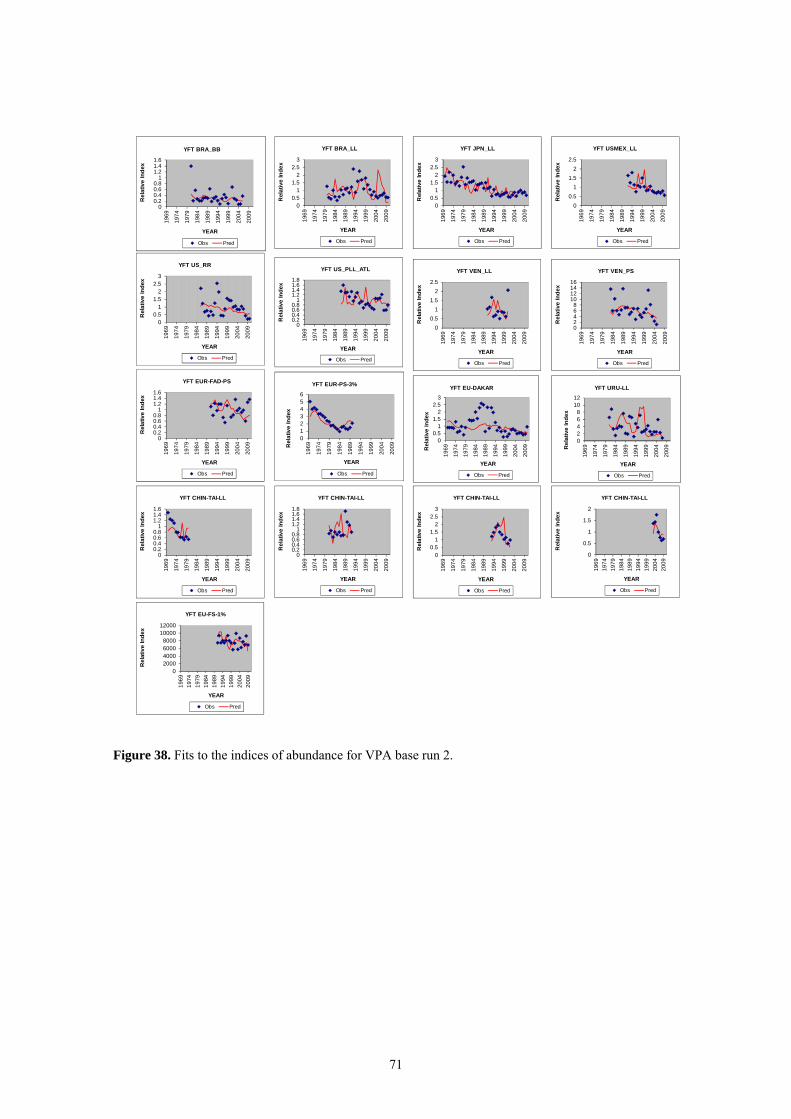
71


00.20.40.60.8

11.21.41.6

196

9

197

4

197

9

198

4

198

9

199

4

199

9

200

4

200

9

Re

lati

ve

Ind

ex

YEAR

YFT BRA_BB

Obs Pred

00.5

11.5

22.5

3

196

9

197

4

197

9

198

4

198

9

199

4

199

9

200

4

200

9

Rel

ati

ve I

nd

ex

YEAR

YFT BRA_LL

Obs Pred

00.5

11.5

22.5

3

196

9

197

4

197

9

198

4

198

9

199

4

199

9

200

4

200

9

Rel

ati

ve I

nd

ex

YEAR

YFT JPN_LL

Obs Pred

0

0.5

1

1.5

2

2.5

196

9

197

4

197

9

198

4

198

9

199

4

199

9

200

4

200

9

Re

lativ

e In

dex

YEAR

YFT USMEX_LL

Obs Pred

00.5

11.5

22.5

3

196

9

197

4

197

9

198

4

198

9

199

4

199

9

200

4

200

9

Re

lati

ve

Ind

ex

YEAR

YFT US_RR

Obs Pred

00.20.40.60.8

11.21.41.61.8

19

69

19

74

19

79

19

84

19

89

19

94

19

99

20

04

20

09

Rel

ati

ve I

nd

ex

YEAR

YFT US_PLL_ATL

Obs Pred

0

0.5

1

1.5

2

2.5

19

69

19

74

19

79

19

84

19

89

19

94

19

99

20

04

20

09

Rel

ati

ve I

nd

ex

YEAR

YFT VEN_LL

Obs Pred

02468

10121416

19

69

19

74

19

79

19

84

19

89

19

94

19

99

20

04

20

09

Rel

ati

ve I

nd

ex

YEAR

YFT VEN_PS

Obs Pred

00.20.40.60.8

11.21.41.6

196

9

197

4

197

9

198

4

198

9

199

4

199

9

200

4

200

9

Re

lativ

e In

dex

YEAR

YFT EUR-FAD-PS

Obs Pred

0123456

196

9

197

4

197

9

198

4

198

9

199

4

199

9

200

4

200

9Re

lativ

e In

dex

YEAR

YFT EUR-PS-3%

Obs Pred

00.5

11.5

22.5

3

19

69

19

74

19

79

19

84

19

89

19

94

19

99

20

04

20

09Re

lati

ve

Ind

ex

YEAR

YFT EU-DAKAR

Obs Pred

02468

1012

196

9

197

4

197

9

198

4

198

9

199

4

199

9

200

4

200

9Re

lati

ve I

nd

ex

YEAR

YFT URU-LL

Obs Pred

00.20.40.60.8

11.21.41.6

196

9

197

4

197

9

198

4

198

9

199

4

199

9

200

4

200

9

Re

lativ

e In

dex

YEAR

YFT CHIN-TAI-LL

Obs Pred

00.20.40.60.8

11.21.41.61.8

196

9

197

4

197

9

198

4

198

9

199

4

199

9

200

4

200

9

Re

lativ

e In

dex

YEAR

YFT CHIN-TAI-LL

Obs Pred

00.5

11.5

22.5

3

196

9

197

4

197

9

198

4

198

9

199

4

199

9

200

4

200

9

Re

lativ

e In

dex

YEAR

YFT CHIN-TAI-LL

Obs Pred

0

0.5

1

1.5

2

196

9

197

4

197

9

198

4

198

9

199

4

199

9

200

4

200

9

Rel

ati

ve I

nd

ex

YEAR

YFT CHIN-TAI-LL

Obs Pred

02000400060008000

1000012000

19

69

19

74

19

79

19

84

19

89

19

94

19

99

20

04

20

09

Re

lati

ve

Ind

ex

YEAR

YFT EU-FS-1%

Obs Pred

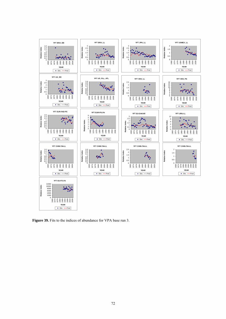
72


00.20.40.60.8

11.21.41.6

19

69

19

74

19

79

19

84

19

89

19

94

19

99

20

04

20

09

Re

lati

ve

In

de

x

YEAR

YFT BRA_BB

Obs Pred

00.5

11.5

22.5

3

19

69

19

74

19

79

19

84

19

89

19

94

19

99

20

04

20

09

Re

lati

ve

In

de

x

YEAR

YFT BRA_LL

Obs Pred

00.5

11.5

22.5

3

19

69

19

74

19

79

19

84

19

89

19

94

19

99

20

04

20

09

Re

lati

ve

In

de

x

YEAR

YFT JPN_LL

Obs Pred

0

0.5

1

1.5

2

19

69

19

74

19

79

19

84

19

89

19

94

19

99

20

04

20

09

Re

lati

ve

In

de

x

YEAR

YFT USMEX_LL

Obs Pred

00.5

11.5

22.5

3

19

69

19

74

19

79

19

84

19

89

19

94

19

99

20

04

20

09

Re

lati

ve

In

de

x

YEAR

YFT US_RR

Obs Pred

00.20.40.60.8

11.21.41.61.8

19

69

19

74

19

79

19

84

19

89

19

94

19

99

20

04

20

09

Re

lati

ve

In

de

x

YEAR

YFT US_PLL_ATL

Obs Pred

0

0.5

1

1.5

2

2.5

19

69

19

74

19

79

19

84

19

89

19

94

19

99

20

04

20

09

Re

lati

ve

In

de

x

YEAR

YFT VEN_LL

Obs Pred

02468

10121416

19

69

19

74

19

79

19

84

19

89

19

94

19

99

20

04

20

09

Re

lati

ve

In

de

x

YEAR

YFT VEN_PS

Obs Pred

00.20.40.60.8

11.21.41.6

19

69

19

74

19

79

19

84

19

89

19

94

19

99

20

04

20

09

Re

lati

ve

In

de

x

YEAR

YFT EUR-FAD-PS

Obs Pred

0123456

19

69

19

74

19

79

19

84

19

89

19

94

19

99

20

04

20

09Re

lati

ve

In

de

x

YEAR

YFT EUR-PS-3%

Obs Pred

00.5

11.5

22.5

3

19

69

19

74

19

79

19

84

19

89

19

94

19

99

20

04

20

09

Re

lati

ve

In

de

x

YEAR

YFT EU-DAKAR

Obs Pred

0

2

4

6

8

10

19

69

19

74

19

79

19

84

19

89

19

94

19

99

20

04

20

09Re

lati

ve

In

de

x

YEAR

YFT URU-LL

Obs Pred

00.20.40.60.8

11.21.41.6

19

69

19

74

19

79

19

84

19

89

19

94

19

99

20

04

20

09

Re

lati

ve

In

de

x

YEAR

YFT CHIN-TAI-LL

Obs Pred

00.20.40.60.8

11.21.41.61.8

19

69

19

74

19

79

19

84

19

89

19

94

19

99

20

04

20

09

Re

lati

ve

In

de

x

YEAR

YFT CHIN-TAI-LL

Obs Pred

0

0.5

1

1.5

2

2.5

19

69

19

74

19

79

19

84

19

89

19

94

19

99

20

04

20

09

Re

lati

ve

In

de

x

YEAR

YFT CHIN-TAI-LL

Obs Pred

0

0.5

1

1.5

2

19

69

19

74

19

79

19

84

19

89

19

94

19

99

20

04

20

09

Re

lati

ve

In

de

x

YEAR

YFT CHIN-TAI-LL

Obs Pred

02000400060008000

1000012000

19

69

19

74

19

79

19

84

19

89

19

94

19

99

20

04

20

09

Re

lati

ve

In

de

x

YEAR

YFT EU-FS-1%

Obs Pred

73


00.20.40.60.8

11.21.41.6

19

69

19

74

19

79

19

84

19

89

19

94

19

99

20

04

20

09

Re

lati

ve

In

de

x

YEAR

YFT BRA_BB

Obs Pred

00.5

11.5

22.5

3

19

69

19

74

19

79

19

84

19

89

19

94

19

99

20

04

20

09

Re

lati

ve

In

de

x

YEAR

YFT BRA_LL

Obs Pred

00.5

11.5

22.5

3

19

69

19

74

19

79

19

84

19

89

19

94

19

99

20

04

20

09

Re

lati

ve

In

de

x

YEAR

YFT JPN_LL

Obs Pred

0

0.5

1

1.5

2

2.5

19

69

19

74

19

79

19

84

19

89

19

94

19

99

20

04

20

09

Re

lati

ve

In

de

x

YEAR

YFT USMEX_LL

Obs Pred

00.5

11.5

22.5

3

19

69

19

74

19

79

19

84

19

89

19

94

19

99

20

04

20

09

Re

lati

ve

In

de

x

YEAR

YFT US_RR

Obs Pred

00.20.40.60.8

11.21.41.61.8

19

69

19

74

19

79

19

84

19

89

19

94

19

99

20

04

20

09

Re

lati

ve

In

de

x

YEAR

YFT US_PLL_ATL

Obs Pred

0

0.5

1

1.5

2

2.5

19

69

19

74

19

79

19

84

19

89

19

94

19

99

20

04

20

09

Re

lati

ve

In

de

x

YEAR

YFT VEN_LL

Obs Pred

02468

10121416

19

69

19

74

19

79

19

84

19

89

19

94

19

99

20

04

20

09

Re

lati

ve

In

de

x

YEAR

YFT VEN_PS

Obs Pred

00.20.40.60.8

11.21.41.6

19

69

19

74

19

79

19

84

19

89

19

94

19

99

20

04

20

09

Re

lati

ve

In

de

x

YEAR

YFT EUR-FAD-PS

Obs Pred

0123456

19

69

19

74

19

79

19

84

19

89

19

94

19

99

20

04

20

09Re

lati

ve

In

de

x

YEAR

YFT EUR-PS-3%

Obs Pred

00.5

11.5

22.5

3

19

69

19

74

19

79

19

84

19

89

19

94

19

99

20

04

20

09

Re

lati

ve

In

de

x

YEAR

YFT EU-DAKAR

Obs Pred

02468

101214

19

69

19

74

19

79

19

84

19

89

19

94

19

99

20

04

20

09Re

lati

ve

In

de

x

YEAR

YFT URU-LL

Obs Pred

00.20.40.60.8

11.21.41.6

19

69

19

74

19

79

19

84

19

89

19

94

19

99

20

04

20

09

Re

lati

ve

In

de

x

YEAR

YFT CHIN-TAI-LL

Obs Pred

00.20.40.60.8

11.21.41.61.8

19

69

19

74

19

79

19

84

19

89

19

94

19

99

20

04

20

09

Re

lati

ve

In

de

x

YEAR

YFT CHIN-TAI-LL

Obs Pred

00.5

11.5

22.5

3

19

69

19

74

19

79

19

84

19

89

19

94

19

99

20

04

20

09

Re

lati

ve

In

de

x

YEAR

YFT CHIN-TAI-LL

Obs Pred

0

0.5

1

1.5

2

19

69

19

74

19

79

19

84

19

89

19

94

19

99

20

04

20

09

Re

lati

ve

In

de

x

YEAR

YFT CHIN-TAI-LL

Obs Pred

02000400060008000

1000012000

19

69

19

74

19

79

19

84

19

89

19

94

19

99

20

04

20

09

Re

lati

ve

In

de

x

YEAR

YFT EU-FS-1%

Obs Pred

74

Retrospective Analysis : Fishing Mortality at Age

Base Run1 Base Run 2 Base Run 3 Base Run 4

Figure 41. Retrospective patterns in fishing mortality at age for the VPA base runs.

75

Retrospective Analysis : Numbers at Age

Base Run1 Base Run 2 Base Run 3 Base Run 4

Figure 42. Retrospective patterns in numbers at age for the VPA base runs.

76

Retrospective Analysis : Spawning Stock Biomass

Figure 43. Retrospective patterns in spawning stock biomass for the VPA base runs.

Figure 44. Jacknife analysis of average fishing mortality, recruits and SSB for the four VPA models obtained by sequential removal of a single index.

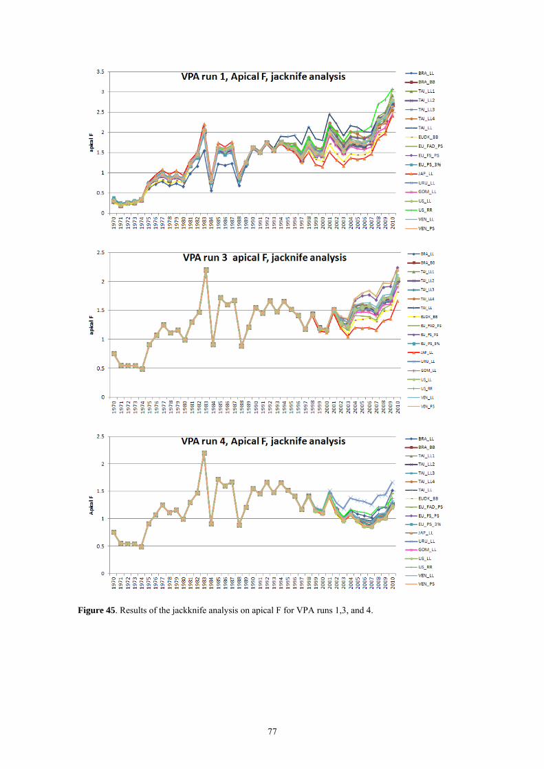
77

Figure 45. Results of the jackknife analysis on apical F for VPA runs 1,3, and 4.

78

Figure 46. Phase plots indicating the median stock status of the VPA base runs (red circle) and the 500 bootstraps analyses.

Figure 47. “Annualized” trajectories of stock status 1972-2010 (i.e., adjusted for the annual selectivity pattern). The 2010 stock status is indicated with a red circle.

79

Figure 48. “Annualized” trajectories of MSY (i.e. adjusted for the annual selectivity pattern) compared to the MSY from VPA-2BOX using the 2006-2010 selectivity pattern.

Figure 49. Phase plots of current stock status by bootstrapped assessment run; the medians for each run are indicated by a grey dot. Quadrants are defined for the stock and fishing mortality relative to BMSY and FMSY; i.e. red B<BMSY and F>FMSY, green red B≥BMSY and F≤FMSY yellow otherwise.

80

Figure 50. Phase plots of current stock status bootstrap results across runs for each method; Production model results (ASPIC) are on the left, and the results of the age-structured model (VPA) are shown on the right. The medians for each method are indicated by a grey dot. Quadrants are defined for the stock amd fishing mortality relative to BMSY and FMSY; i.e. red B<BMSY and F>FMSY, green red B≥BMSY and F≤FMSY yellow otherwise.

Figure 51. Biomass ratios and fishing mortality ratios describing current stock status from the combined joint distribution of ASPIC and VPA base case runs. Points represent a total of 4000 bootstraps. The median of the joint distribution is indicated by a grey dot. Quadrants are defined for the stock and fishing mortality relative to BMSY and FMSY; i.e. red B<BMSY and F>FMSY, green red B≥BMSY and F≤FMSY yellow otherwise.

81

a) – Number of vessels by category (TRB) b) – Number of 1ºx1º CWP explored by effort level

c) – Carrying Capacity and fishing days (fishing day=12 hours) d) – Number of sets and percentage of nul sets by fishing mode (FAD (BO) and free school (BL))

Figure 52. Fishing effort of the European and associated purse seine fleet : a) Number of vessels by TRB category, b) Number of 1ºx1º CWP explored , c) Carrying capacity in tones and fishing days , d) Number of sets and percentage of nul sets by fishing mode.

0

25

50

75

1991 1993 1995 1997 1999 2001 2003 2005 2007 2009

Nu

mb

er o

f ve

ssel

s

50-400 401-600 601-800801-1200 1201-2000 total

0

200

400

600

800

1000

1991 1993 1995 1997 1999 2001 2003 2005 2007 2009

Nu

mb

er o

f 1º

x1º

CW

P

Visités Avec au moins une caléeAvec des capture Avec un effort > 12hAvec un effort > 60h

0

5

10

15

20

25

0

10

20

30

40

50

1991 1993 1995 1997 1999 2001 2003 2005 2007 2009N

um

ber

of

day

s (x

1000

)

Car

ryin

g C

apac

ity

(x10

00)

Capacité de transport Jours de pêcheJours de recherche

0%

20%

40%

60%

80%

0.0

2.0

4.0

6.0

8.0

1991 1993 1995 1997 1999 2001 2003 2005 2007 2009Nu

mb

er o

f se

ts (

x100

0)Objets Libre % Nuls BO % Nuls BL

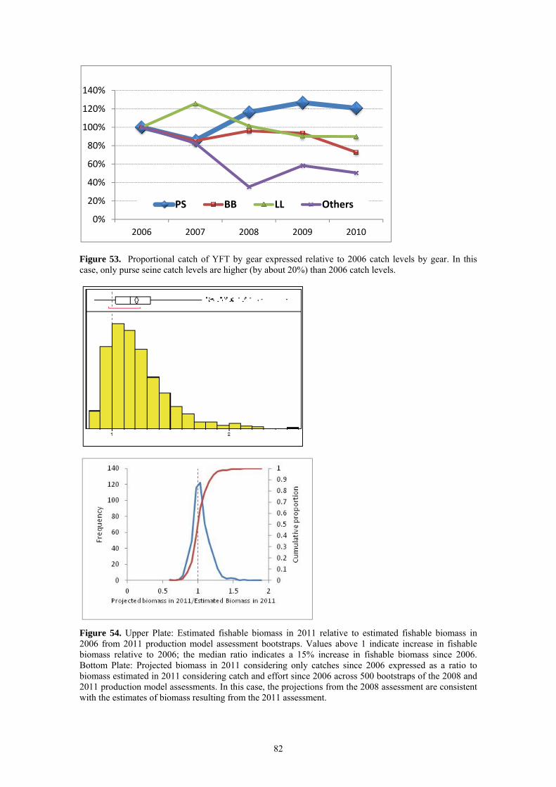
82

Figure 53. Proportional catch of YFT by gear expressed relative to 2006 catch levels by gear. In this case, only purse seine catch levels are higher (by about 20%) than 2006 catch levels.

Figure 54. Upper Plate: Estimated fishable biomass in 2011 relative to estimated fishable biomass in 2006 from 2011 production model assessment bootstraps. Values above 1 indicate increase in fishable biomass relative to 2006; the median ratio indicates a 15% increase in fishable biomass since 2006. Bottom Plate: Projected biomass in 2011 considering only catches since 2006 expressed as a ratio to biomass estimated in 2011 considering catch and effort since 2006 across 500 bootstraps of the 2008 and 2011 production model assessments. In this case, the projections from the 2008 assessment are consistent with the estimates of biomass resulting from the 2011 assessment.

0%

20%

40%

60%

80%

100%

120%

140%

2006 2007 2008 2009 2010

PS BB LL Others

83

Figure 55. Estimated spawning stock biomass from the age-structured analysis indicating recent declines. Histograms on the right represent the bootstrap outcomes from the analysis

Figure 56. ASPIC projections of median biomass ratios for runs 09, 10, 11 and 12. Projections are conducted from 2011 until 2025. Catch levels vary from 50,000 until 150,000 t in 10,000 steps.

20000

40000

60000

80000

100000

120000

140000

Dat

a

2006 2007 2008 2009 2010 2011

Label

2006 2007 2008 2009 2010 2011

0

1

2

2011

2012

2013

2014

2015

2016

2017

2018

2019

2020

2021

2022

2023

2024

2025

B/B

msy

Run11

50000MT

60000MT

70000MT

80000MT

90000MT

100000MT

110000MT

120000MT

130000MT

140000MT

150000MT

0

1

2 20

11

2012

2013

2014

2015

2016

2017

2018

2019

2020

2021

2022

2023

2024

2025

B/B

msy

Run09

50000MT

60000MT

70000MT

80000MT

90000MT

100000MT

110000MT

120000MT

130000MT

14000MT

150000MT

0

1

2

2011

2012

2013

2014

2015

2016

2017

2018

2019

2020

2021

2022

2023

2024

2025

B/B

msy

Run10

50000MT

60000MT

70000MT

80000MT

90000MT

100000MT

110000MT

120000MT

130000MT

140000MT

150000MT

0

1

2

2011

2012

2013

2014

2015

2016

2017

2018

2019

2020

2021

2022

2023

2024

2025

B/B

msy

Run12

50000MT

60000MT

70000MT

80000MT

90000MT

100000MT

110000MT

120000MT

130000MT

140000MT

150000MT

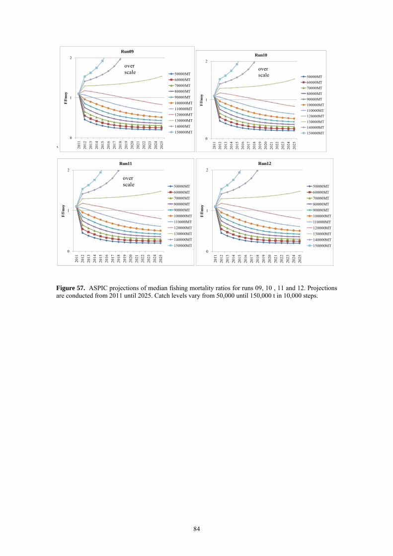
84

`

Figure 57. ASPIC projections of median fishing mortality ratios for runs 09, 10 , 11 and 12. Projections are conducted from 2011 until 2025. Catch levels vary from 50,000 until 150,000 t in 10,000 steps.

0

1

2

2011

2012

2013

2014

2015

2016

2017

2018

2019

2020

2021

2022

2023

2024

2025

F/Fm

sy

Run09

50000MT

60000MT

70000MT

80000MT

90000MT

100000MT

110000MT

120000MT

130000MT

14000MT

150000MT

over scale

0

1

2

2011

2012

2013

2014

2015

2016

2017

2018

2019

2020

2021

2022

2023

2024

2025

F/Fm

sy

Run10

50000MT

60000MT

70000MT

80000MT

90000MT

100000MT

110000MT

120000MT

130000MT

140000MT

150000MT

over scale

0

1

2

2011

2012

2013

2014

2015

2016

2017

2018

2019

2020

2021

2022

2023

2024

2025

F/Fm

sy

Run11

50000MT

60000MT

70000MT

80000MT

90000MT

100000MT

110000MT

120000MT

130000MT

140000MT

150000MT

over scale

0

1

2

2011

2012

2013

2014

2015

2016

2017

2018

2019

2020

2021

2022

2023

2024

2025

F/Fm

sy

Run12

50000MT

60000MT

70000MT

80000MT

90000MT

100000MT

110000MT

120000MT

130000MT

140000MT

150000MT

85

Figure 58. Projection results for the VPA RUN 1 base case.

0

100000

200000

300000

400000

500000

600000

700000

800000

900000

1000000

2005 2010 2015 2020

Total Biomass (m

t)

YEAR

Total Biomass (mt)

50,000 mt

70,000 mt

90,000 mt

110,000 mt

120,000 mt

130,000 mt

150,000 mt

0

10000000

20000000

30000000

40000000

50000000

60000000

70000000

2005 2010 2015 2020

Recruits

YEAR

Recruits

50,000 mt

70,000 mt

90,000 mt

110,000 mt

120,000 mt

130,000 mt

150,000 mt

0

20000000

40000000

60000000

80000000

100000000

120000000

140000000

160000000

2005 2010 2015 2020

Yield (mt)

YEAR

Yield (mt)

150,000 mt

110,000 mt

120,000 mt

130,000 mt

90,000 mt

70,000 mt

50,000 mt

0

1

2

3

4

5

6

2005 2010 2015 2020

Apical F

YEAR

Apical F

150,000mt130,000mt120,000mt110,000mt90,000 mt

70,000 mt

0

100000

200000

300000

400000

500000

600000

2005 2010 2015 2020

Spaw


t)

YEAR


50,000 mt

70,000 mt

90,000 mt

110,000 mt

120,000 mt

130,000 mt

150,000 mt

SSBmsy

86


0

200000

400000

600000

800000

1000000

1200000

2005 2010 2015 2020

Total Biomass (m

t)

YEAR

Total Biomass (mt)

50,000 mt

70,000 mt

90,000 mt

110,000 mt

120,000 mt

130,000 mt

150,000 mt

0

10000000

20000000

30000000

40000000

50000000

60000000

70000000

2005 2010 2015 2020

Recruits

YEAR

Recruits

50,000 mt

70,000 mt

90,000 mt

110,000 mt

120,000 mt

130,000 mt

150,000 mt

0

20000000

40000000

60000000

80000000

100000000

120000000

140000000

160000000

2005 2010 2015 2020

Yield (mt)

YEAR

Yield (mt)

150,000 mt

110,000 mt

120,000 mt

130,000 mt

90,000 mt

70,000 mt

50,000 mt

0

1

2

3

4

5

6

2005 2010 2015 2020

Apical F

YEAR

Apical F

150,000mt130,000mt120,000mt110,000mt90,000 mt

70,000 mt

0

100000

200000

300000

400000

500000

600000

2005 2010 2015 2020

Spaw


t)

YEAR


50,000 mt

70,000 mt

90,000 mt

110,000 mt

120,000 mt

130,000 mt

150,000 mt

SSBmsy

87


0

100000

200000

300000

400000

500000

600000

700000

800000

900000

1000000

2005 2010 2015 2020

Total Biomass (m

t)

YEAR

Total Biomass (mt)

50,000 mt

70,000 mt

90,000 mt

110,000 mt

120,000 mt

130,000 mt

150,000 mt

0

10000000

20000000

30000000

40000000

50000000

60000000

70000000

2005 2010 2015 2020

Recruits

YEAR

Recruits

50,000 mt

70,000 mt

90,000 mt

110,000 mt

120,000 mt

130,000 mt

150,000 mt

0

20000000

40000000

60000000

80000000

100000000

120000000

140000000

160000000

2005 2010 2015 2020

Yield (mt)

YEAR

Yield (mt)

150,000 mt

110,000 mt

120,000 mt

130,000 mt

90,000 mt

70,000 mt

50,000 mt

0

1

2

3

4

5

6

2005 2010 2015 2020

Apical F

YEAR

Apical F

150,000mt130,000mt120,000mt110,000mt90,000 mt

70,000 mt

0

100000

200000

300000

400000

500000

600000

2005 2010 2015 2020

Spaw


t)

YEAR


50,000 mt

70,000 mt

90,000 mt

110,000 mt

120,000 mt

130,000 mt

150,000 mt

SSBmsy

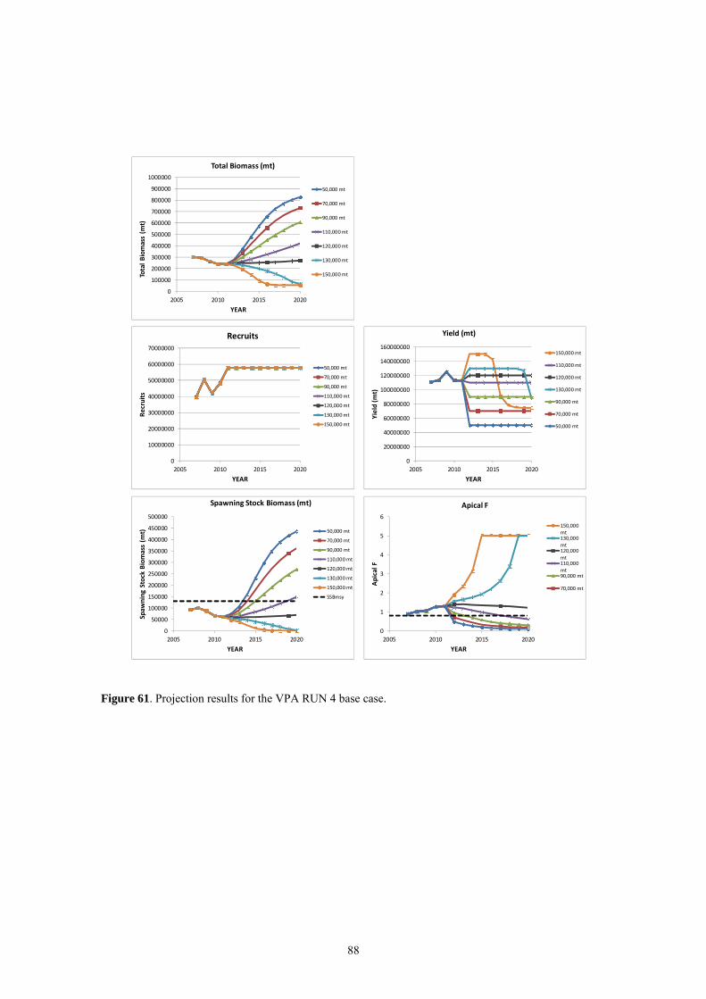
88


0

100000

200000

300000

400000

500000

600000

700000

800000

900000

1000000

2005 2010 2015 2020

Total Biomass (m

t)

YEAR

Total Biomass (mt)

50,000 mt

70,000 mt

90,000 mt

110,000 mt

120,000 mt

130,000 mt

150,000 mt

0

10000000

20000000

30000000

40000000

50000000

60000000

70000000

2005 2010 2015 2020

Recruits

YEAR

Recruits

50,000 mt

70,000 mt

90,000 mt

110,000 mt

120,000 mt

130,000 mt

150,000 mt

0

20000000

40000000

60000000

80000000

100000000

120000000

140000000

160000000

2005 2010 2015 2020

Yield (mt)

YEAR

Yield (mt)

150,000 mt

110,000 mt

120,000 mt

130,000 mt

90,000 mt

70,000 mt

50,000 mt

0

1

2

3

4

5

6

2005 2010 2015 2020

Apical F

YEAR

Apical F

150,000mt130,000mt120,000mt110,000mt90,000 mt

70,000 mt

0

50000

100000

150000

200000

250000

300000

350000

400000

450000

500000

2005 2010 2015 2020

Spaw


t)

YEAR


50,000 mt

70,000 mt

90,000 mt

110,000 mt

120,000 mt

130,000 mt

150,000 mt

SSBmsy

89

Appendix 1

AGENDA

1. Opening, adoption of the Agenda and meeting arrangements

2. Review of Biological historical and new data.

3. Review of basic information

2.1 Task I (catches) 2.2 Task II (catch-effort and size samples) 2.3 Other information (tagging)

5. Review of catch per unit effort series and other fishery indicators

6. Conversion of catch-at-size to catch-at-age

7. Stock assessment

7.1 Methods and other data relevant to the assessment 7.2 Stock status 7.3 Projections

8. Evaluation of management scenarios

9. Recommendations

9.1 Research and statistics 9.2 Management

10. Other matters

11. Adoption of the report and closure

Appendix 2

LIST OF PARTICIPANTS SCRS CHAIRMAN Santiago Burrutxaga, Josu Head of Tuna Research Area, AZTI-Tecnalia, Txatxarramendi z/g, 48395 Sukarrieta (Bizkaia), Spain Tel: +34 94 6574000 (Ext. 497); 664303631, Fax: +34 94 6572555, E-Mail: [email protected] CONTRACTING PARTIES BRAZIL Agrelli Andrade, Humber Universidade Federal de Santa Catarina - UFSC Depto. Informática e Estatística,INE/CTC Caixa Postal 476, Florianópolis Santa Catarina Tel: + 55 48 3721 9942, Fax: + 55 48 3721 9566, E-Mail: [email protected]; [email protected] EUROPEAN UNION Ariz Tellería, Javier Ministerio de Ciencia e Innovación Instituto Español de Oceanografía, C.O. de Canarias, Apartado 1373, 38080 Santa Cruz de Tenerife, Islas Canarias, Spain Tel: +34 922 549 400, Fax: +34 922 549 554, E-Mail: [email protected] De Bruyn, Paul AZTI - Tecnalia,Herrera Kaia Portualdea z/g, 20110 Pasaia Gipuzkoa, Spain Tel: +34 94 657 40 00, Fax: +34 946 572 555, E-Mail: [email protected] Chassot, Emmanuel IRD, Centre de Recherche Halieutique Méditerranéenne et Tropicale, Ave. Jean Monnet, B.P. 171, 34203 Sète Cedex, France Tel: +33 499 573 224, Fax: +33 4 99 573 295, E-Mail: [email protected]

90

Delgado de Molina Acevedo, Alicia Ministerio de Ciencia e Innovación Instituto Español de Oceanografía, C.O. de Canarias, Apartado 1373, 38080 Santa Cruz de Tenerife Islas Canarias, Spain Tel: +34 922 549 400, Fax: +34 922 549 554, E-Mail: [email protected] Gaertner, Daniel I.R.D. UR No. 109 Centre de Recherche Halieutique Méditerranéenne et Tropicale, Avenue Jean Monnet - B.P. 171, 34203 Sète Cedex, France Tel: +33 4 99 57 32 31, Fax: +33 4 99 57 32 95, E-Mail: [email protected] Murua, Hilario AZTI - Tecnalia /Itsas Ikerketa Saila,Herrera Kaia Portualde z/g, 20110 Pasaia Gipuzkoa, Spain Tel: +34 94 657 40 00, Fax: +34 943 004801, E-Mail: [email protected] Pereira, Joao Gil Universidade dos Açores, Departamento de Oceanografia e Pescas, 9900 Horta, Portugal Tel: +351 292 207 806, Fax: +351 292 207811, E-Mail: [email protected] JAPAN Ijima, Hirotaka Associate Researcher, Tuna Fisheries Resources Group; Tuna an Skipjack Resources Division, National Research Institute of Far Seas Fisheries, 5-7-1, Chome Orido, Shizuoka-Shi Shimizu-Ku 424-8633 Tel: +81 543 36 6044, Fax: +81 543 35 9642, E-Mail: Satoh, Keisuke Tropical Tuna Section, Tuna and Skipjack Resources Division, National Research Institute of Far Seas Fisheries, Fisheries Research Agency of Japan, 7-1, 5 Chome Orido, Shizuoka-Shi Shimizu-Ku Tel: +81 543 36 6044, Fax: +81 543 35 9642, E-Mail: [email protected] SENEGAL Ngom Sow, Fambaye Chargé de Recherches, Centre de Recherches Océanographiques de Dakar Thiaroye, CRODT/ISRA, LNERV, Route du Front de Terre, B.P. 2241, Dakar Tel: +221 33 832 8265, Fax: +221 33 832 8262, E-Mail: [email protected] UNITED STATES Brown, Craig A. NOAA Fisheries Southeast Fisheries Center, Sustainable Fisheries Div., 75 Virginia Beach Drive, Miami, Florida 33149 Tel: +1 305 361 4590, Fax: +1 305 361 4562, E-Mail: [email protected] Cass-Calay, Shannon NOAA Fisheries, Southeast Fisheries Center, Sustainable Fisheries Div., 75 Virginia Beach Drive, Miami, Florida 33149 Tel: +1 305 361 4231, Fax: +1 305 361 4562, E-Mail: [email protected] Díaz, Guillermo Office of Science and Technology (ST4), National Marine Fisheries Service, 1315 East-West Highway, Silver Spring, Maryland 20910 Tel: +1 301 713 2363, Fax: +1 301 713 1875, E-Mail: [email protected] Die, David Cooperative Unit for Fisheries Education and Research University of Miami, 4600 Rickenbacker Causeway, Miami, Florida 33149 Tel: +1 305 421 4607, Fax: +1 305 421 4221, E-Mail: [email protected] Scott, Gerald P. SCRS Chairman, NOAA Fisheries, Southeast Fisheries Science Center Sustainable Fisheries Division, 75 Virginia Beach Drive, Miami, Florida 33149 Tel: +1 305 361 4261, Fax: +1 305 361 4219, E-Mail: [email protected] Walter, John NOAA Fisheries, Southeast Fisheries Center, Sustainable Fisheries Division, 75 Virginia Beach Drive, Miami, Florida 33149 Tel: +305 365 4114, Fax: +1 305 361 4562, E-Mail: [email protected]

91

OBSERVERS FROM COOPERATING NON-CONTRACTING PARTIES, ENTITIES, FISHING ENTITIES SURINAME REP. Lieveld, Rene Deputy Director of Fisheries of Surinam

**********

ICCAT SECRETARIAT C/ Corazón de María, 8 - 6 Planta, 28002 Madrid, Spain

Tel: + 34 91 416 5600, Fax: +34 91 415 2612, E-Mail: [email protected]

Kell, Laurie Ortiz, Mauricio Palma, Carlos Pallarés, Pilar

Appendix 3

LIST OF DOCUMENTS SCRS/2010/090 Analysis of the catch rate of juvenile bigeye depending on the depth of the purse seine net

used by the tropical fleet. Delgado de Molina, A., Ariz, J., Santana, J.C. and Sotillo, B.

SCRS/2011/087 Review of the available Ghana statistics on tropical fisheries. Palma C., Pallares P., Ortiz, M. and Kell, L.

SCRS/2011/127 Attempt to modify creating procedure of catch-at-size of yellowfin caught by Japanese longline tuna fishery in the Atlantic Ocean. Ijima, H., Satoh, K., Okamoto, H.

SCRS/2011/128 Japanese longline CPUE for yellowfin tuna (Thunnus albacares) in the Atlantic Ocean using GLM up to 2010. Satoh, K., Okamoto, H., Ijima, H.

SCRS/2011/129 Standardized abundance index of yellowfin tuna by the Taiwanese longline fleet in the Atlantic Ocean for 1968-2009. Hus, C.C.

SCRS/2011/130 Estadísticas españolas de la pesquería atunera tropical en el océano Atlántico hasta 2010. Delgado de Molina, A., Ariz, J., Santana, J.C. y Sabaté, I.

SCRS/2011/131 Datos estadísticos de la pesquería de túnidos de las Islas Canarias durante el periodo 1975 a 2010. Delgado de Molia, A., Delgado de Molina, R., Santana, J.C. y Ariz. J.

SCRS/2011/136 Statistics of the French purse seine fleet targeting tropical tunas in the Atlantic Ocean (1991-2010). Floch, L., Chassot, E., Damiano, A., Kouassi, Y., Pianet, R. and Chavance, P.

SCRS/2011/137 Statistiques de la pêcherie thonière Europeenne et assimilée dans l’océan Atlantique durant la période 1991-2010. Pianet, R., Delgado, A., Floch, L., Ariz, A., Damiano, A., Sabate, I., Kouassi, Y. et N’Gom Sow, F.

SCRS/2011/138 Standardized catch rates for yellowfin tuna (Thunnus albacares) from the U.S. pelagic longline fishery based upon vessel logbook data (1990-2010). Walter, J.F.

SCRS/2011/139 Standardized catch rates for yellowfin tuna (Thunnus albacares) from the U.S. recreational fishery in the western North Atlantic Ocean, 1986-2010. Cass-Calay, S.L., Walter, J.F. and Brown, C.A.

SCRS/2011/140 Standardized catch rates for yellowfin tuna (Thunnus albacares) in the Gulf of Mexico longline fishery for 1992-2010 based upon observer programs from Mexico and the United States. Brown, C. and Ramírez-López K.

SCRS/2011/141 Preliminary analysis of time spent at temperature relative to the surface temperature for yellowfin tuna monitored with pop-up satellite archival tags in the Gulf of Mexico. Hoolihan, J.P., Wells, R.J.D., Luo, J., Rooker, J.R. and Prince E.D.

92

SCRS/2011/142 Review ageing protocols for Atlantic yellowfin tuna (Thunnus albacares). Ortiz, M. and Palma, C.

SCRS/2011/143 Fishery analysis of yellowfin caught by Cabo Frio, Rio de Janeiro-Brazil small-size fleet (2003-2010). Pimenta, E.G., Rezende, M., Hazin, H.G., Hazin, F.H.V. and Amorim, A.F.

SCRS/2011/144 Standardization of a CPUE series of yelowfin tuna, Thunnus albacares, caught by Brazilian longliners in the southwestern Atlantic Ocean by generalized linear mixed models. Hazin, H., Hazin, F.H.V., Amorim, C.A., Travassos, P., Freduo, T.

SCRS/2011/145 Preliminary results on the catch composition in small-scale tuna fisheries associated to an offshore buoy in the western equatorial Atlantic. Silva, G.B., Azevedo, D.V.D., Chaves, D. C.B., Fonteles-Filho, A.A., Hazin, H.

SCRS/2011/146 An evaluation of a harvest control rule based on limits and targets: An example based on yellowfin tuna. Kell, L., Magnusson, De Bruyn, P. and Mosqueira, I.

SCRS/2011/147 An evaluation of the performance of the Kobe Strategy Matrix; An example based upon a biomass dynamic assessment mode. Kell, L., Magnusson, A., De Bruyn, P. and Mosqueira, I.

SCRS/2011/148 A Kobe Strategy Matrix Based upon Probabilistic Reference Points; An Example Using a Biomass Dynamic Assessment Model. Kell, L., Magnusson, A., De Bruyn, P. and Mosqueira, I.

Appendix 4

Estimation of Combined Indexes Combined indexes were estimated using a GLM approach with the following model formulation:

Log(index) = Year + Source + ε Where ‘Source’ identifies the index (fleet) included in the model and ε is the error term. Original indexes estimated as number of fish per unit of effort were transformed into biomass by multiplying the index value times the fleet specific annual average weight of the fish estimated from catch-at-size data expanded to the Task I data (file SOP_casYFT7010_v2.xsls provided by the Secretariat). Annual weighting factors (Table Appendix 4.1) were estimated for each fleet by counting the number of 5ox5o squares where each fishery operated and estimating the proportion to the total number of squares fished for each year. This approach allowed capturing the spatial expansion/contraction experienced by different fleets over time. The index weights were re-scaled so that they would add up to 1.0 each year. Four different combined indexes were estimated. Values of the indexes used as input for the estimation of the different combined indexes are presented in Table Appendix 4.2. When possible, the input indexes were scaled to their respective mean value for the period 1993-2001. The first estimated combined index (Index 1) was prepared to run in the ASPIC continuity case. The 13 indexes used to estimate this combined index were the following:

Fleet Period

Japan longline 1965-2010

Gulf of Mexico longline 1993-2010

U.S. rod and reel recreational 1986-2010

Brazil longline 1986-2006

Uruguay longline 1981-2006

Chinese Taipei longline 1968-2009

93

Canarias Islands baitboat 1980-2006

Venezuela purse seine 1983-2005

Brazil baitboat 1981-2006

U.S. longline (Atl. only) 1987-2010

EU Dakar baitboat 1969-2010

Venezuela longline 1991-2001

EU purse seine 3% 1970-2010

A second combined index (Index 2) was estimated by replacing the Brazil Longline index with an updated version that covered the period 1980-2010 and by splitting the Chinese Taipei into 4 different time periods (and, therefore, defining 4 new different fisheries): 1968-1980, 1981-1992, 1993-2002, and 2003-2009. However, by splitting the Chinese Taipei series into four different series, it was not possible to scale all of them to their mean value of the period 1993-2001. To scale those Chinese Taipei series that did not overlap with 1993-2001, an average value for all scaled series in each one of those time periods was estimated. The average value of the un-scaled Chinese Taipei index for that time period was then divided by the estimated average for the other fleets. Finally, each individual value of the Chinese Taipei index was divided by the ratio obtained in the previous step. The third index (Index 3) was constructed with the same indexes used in the second case except for the EU purse seine index with a 3% increase in catchability (EU PS 3%). The original EU PS 3% covered the entire period 1970-2010. For this index only the period 1970-1990 was used, and for the period 1991-2010 two new indexes were introduced: an EU PS (free school) with a 1% increase in catchability and an EU-Spain PS FAD. Both new indexes were equally weighted using the same weighting factors previously applied to the EU PS 3% index. The final combined index (Index 4) used the same indexes as in the third case, except that the EU PS 3% was replaced by an EU PS 7% index. All weighted combined indexes are shown in Figure Appendix 4.1 and their values are presented in Table Appendix 4.3. To better assess the influence of some indexes on the combined index (fourth case), 3 combined indexes were estimated by removing the Chinese Taipei (all four series), the Brazil Longline, and the EU PS 7% together with the EU PS 1% and the EU-Spain PS FAD indexes one at the time. The results indicated that of all those indexes, the Chinese Taipei index had the biggest influence of the estimated combine index (Figure Appendix 4.2).

94

Table Appendix 4.1. Weighting factors used in the calculation of the different combined indexes.

LL BB PS

Year JAP BRA Chi-Tai GOM USA Atl URU VEN BRA DKR CAN US RR

EU PS 3% VEN

1965 1 1966 1 1967 1 1968 0.6580 0.3420 1969 0.4723 0.4383 0.0894 1970 0.4946 0.4219 0.0835 1971 0.5393 0.3081 0.0770 0.0756 1972 0.4808 0.3276 0.0843 0.1073 1973 0.4444 0.3171 0.1003 0.1382 1974 0.3778 0.4099 0.0815 0.1309 1975 0.5011 0.3244 0.0492 0.1253 1976 0.3869 0.4453 0.0389 0.1290 1977 0.3366 0.4703 0.0421 0.1510 1978 0.3451 0.4457 0.0299 0.1793 1979 0.4265 0.3529 0.0500 0.1706 1980 0.4038 0.3654 0.0470 0.0171 0.1325 0.0342 1981 0.4241 0.3298 0.0070 0.0297 0.0070 0.0140 0.1606 0.0279 1982 0.4360 0.3316 0.0067 0.0354 0.0067 0.0135 0.1431 0.0269 1983 0.3779 0.2939 0.0076 0.0305 0.0382 0.0153 0.1947 0.0420 1984 0.4032 0.2842 0.0071 0.0586 0.0355 0.0142 0.1208 0.0764 1985 0.4438 0.2695 0.0058 0.0461 0.0173 0.0115 0.0965 0.1095 1986 0.3705 0.0372 0.3497 0.0060 0.0268 0.0253 0.0119 0.0595 0.0967 0.0164 1987 0.3305 0.0470 0.2564 0.1396 0.0057 0.0356 0.0171 0.0114 0.0570 0.0855 0.0142 1988 0.3959 0.0509 0.1063 0.1907 0.0058 0.0320 0.0291 0.0116 0.0582 0.1063 0.0131 1989 0.4401 0.0404 0.0952 0.1905 0.0058 0.0390 0.0231 0.0115 0.0577 0.0851 0.0115 1990 0.4149 0.0432 0.1432 0.1676 0.0054 0.0311 0.0270 0.0108 0.0541 0.0878 0.0149 1991 0.3638 0.0509 0.2380 0.1008 0.0042 0.0062 0.0239 0.0125 0.0083 0.0416 0.1414 0.0083 1992 0.3072 0.0937 0.1667 0.1155 0.0044 0.0065 0.0370 0.0163 0.0087 0.0436 0.1863 0.0142 1993 0.2522 0.1429 0.1970 0.0236 0.1044 0.0039 0.0069 0.0266 0.0099 0.0079 0.0394 0.1724 0.0128 1994 0.2733 0.1320 0.2422 0.0226 0.0924 0.0038 0.0075 0.0160 0.0113 0.0075 0.0377 0.1433 0.0104 1995 0.2700 0.1240 0.2181 0.0211 0.1003 0.0035 0.0070 0.0176 0.0132 0.0070 0.0352 0.1733 0.0097 1996 0.2693 0.0873 0.2702 0.0223 0.0947 0.0037 0.0074 0.0149 0.0139 0.0074 0.0371 0.1606 0.0111 1997 0.2814 0.0932 0.2690 0.0228 0.1093 0.0038 0.0076 0.0095 0.0124 0.0076 0.0380 0.1369 0.0086 1998 0.2647 0.1373 0.2683 0.0214 0.1007 0.0036 0.0062 0.0143 0.0080 0.0071 0.0357 0.1275 0.0053 1999 0.2301 0.2190 0.2827 0.0204 0.0628 0.0034 0.0195 0.0042 0.0102 0.0068 0.0340 0.0985 0.0085 2000 0.2619 0.1456 0.3166 0.0185 0.0562 0.0031 0.0254 0.0108 0.0108 0.0062 0.0308 0.1063 0.0077 2001 0.2652 0.1518 0.2700 0.0192 0.0615 0.0032 0.0264 0.0112 0.0096 0.0064 0.0319 0.1350 0.0088

95

2002 0.2093 0.2257 0.3034 0.0196 0.0564 0.0033 0.0147 0.0114 0.0065 0.0327 0.1112 0.0057 2003 0.2621 0.1379 0.2825 0.0233 0.0485 0.0039 0.0350 0.0146 0.0078 0.0388 0.1369 0.0087 2004 0.2389 0.1639 0.3114 0.0198 0.0445 0.0033 0.0371 0.0115 0.0066 0.0329 0.1219 0.0082 2005 0.1988 0.1715 0.2471 0.0163 0.0980 0.0027 0.1307 0.0095 0.0054 0.0272 0.0803 0.0123 2006 0.2510 0.2181 0.2693 0.0232 0.0569 0.0039 0.0290 0.0106 0.0077 0.0386 0.0917 2007 0.2354 0.1188 0.2915 0.0269 0.0650 0.0045 0.0370 0.0157 0.0090 0.0448 0.1513 2008 0.2639 0.1298 0.2425 0.0258 0.0590 0.0086 0.0279 0.0236 0.0086 0.0429 0.1674 2009 0.2639 0.1298 0.2425 0.0258 0.0590 0.0086 0.0279 0.0236 0.0086 0.0429 0.1674 2010 0.2639 0.1298 0.2425 0.0258 0.0590 0.0086 0.0279 0.0236 0.0086 0.0429 0.1674

96

Table Appendix 4.2. Indices of abundance in weight used to estimate the different combined. The indexes were scaled to the mean values of the period 1993-2001 (see text for details).

Year JAP GOM USA BRA URU TAI CAN VEN BRA USA EUDKR VEN EU BRA EU EU EU

LL LL RR LL LL LL BB PS BB LL BB LL PS 3% LL PS 1% PS FAD PS 7%

1965 3.87 1966 2.69 1967 5.30 1968 4.34 3.16 1969 3.81 2.33 1.20 1970 2.87 1.46 1.16 1.47 2.943 1971 2.38 1.05 1.15 1.25 2.347 1972 3.17 0.78 1.16 1.39 2.435 1973 2.13 0.73 1.07 1.40 2.294 1974 3.03 0.44 1.65 1.28 1.954 1975 2.19 0.42 0.74 1.37 1.967 1976 2.27 0.42 0.83 1.36 1.818 1977 1.77 0.36 1.23 1.34 1.669 1978 2.59 0.28 0.50 1.22 1.420

1979 3.13 0.36 1.13 1.21 1.319 1980 1.89 0.00 0.27 0.05 0.00 1.00 0.945 1.022 1981 2.46 1.40 0.60 0.10 4.47 1.83 1.07 0.263 1.055 1982 2.14 1.90 0.66 0.50 0.68 1.74 0.92 0.267 0.867 1983 2.06 0.82 0.50 0.88 2.20 1.85 1.77 0.80 0.609 0.725 1984 2.23 0.41 0.63 3.27 0.98 0.90 2.52 0.63 0.260 0.551 1985 1.46 0.73 0.54 1.42 1.65 0.67 1.94 1.08 0.193 0.912 1986 1.83 1.42 1.39 1.12 0.57 0.91 0.97 0.67 2.91 1.17 0.377 0.947 1987 1.91 0.78 1.76 1.08 0.45 2.04 0.74 0.95 1.77 3.27 1.02 0.647 0.798 1988 1.91 0.37 1.46 1.38 0.48 2.13 1.02 1.05 2.11 3.16 0.97 0.306 0.728 1989 1.53 0.64 1.48 0.55 1.26 1.26 2.21 0.96 1.68 0.79 1.21 0.486 0.873 1990 1.99 0.27 2.50 0.50 1.12 3.20 1.13 1.99 1.62 2.92 1.31 0.738 1.211 1991 1.54 0.43 1.37 1.80 0.75 2.83 1.16 0.60 1.37 1.08 1.11 1.24 0.521 0.973 1.138 1992 1.76 1.46 0.29 0.57 2.83 0.67 1.64 0.78 0.95 1.60 2.91 1.63 1.13 0.513 1.220 0.837 1993 0.84 1.12 0.77 0.66 0.54 0.83 0.75 0.89 1.12 0.90 2.48 2.35 1.08 2.388 0.979 1.265 1994 1.39 1.51 1.97 0.74 2.07 1.10 0.45 1.09 0.67 0.85 1.60 1.12 1.06 0.549 1.042 0.995 1995 1.01 0.99 2.47 0.50 0.85 1.26 0.19 0.49 0.33 1.32 0.91 0.77 1.06 0.837 0.972 1.231 1996 1.08 0.67 0.58 1.29 1.61 1.48 2.85 1.10 0.93 1.23 1.13 0.98 1.01 1.172 1.048 1.235 1997 0.83 0.96 0.26 1.02 0.53 1.19 0.34 0.74 1.35 1.09 0.79 0.60 0.94 0.861 1.224 0.754 1998 0.97 0.81 0.46 1.30 0.60 1.00 4.03 0.60 1.04 0.71 0.33 1.02 0.99 0.557 1.051 0.573 1999 1.01 1.20 0.77 1.22 1.21 0.81 0.38 0.88 0.36 1.00 0.83 0.93 0.82 1.070 0.978 1.179 2000 1.11 0.90 0.86 1.27 1.60 0.80 0.01 1.07 0.00 0.96 0.37 0.29 0.97 0.929 0.744

97

2001 0.75 0.84 0.84 1.02 0.54 0.00 2.14 2.19 0.94 0.57 0.95 1.06 0.637 0.961 0.767 2002 0.75 0.82 0.74 0.80 0.97 0.79 0.13 1.32 0.93 0.64 0.97 1.16 0.535 1.295 0.848 2003 0.90 1.07 0.64 1.71 1.47 1.09 0.24 0.65 0.76 0.53 1.02 1.08 0.891 0.755 1.408 2004 1.16 0.76 0.57 2.08 1.06 1.21 0.20 0.39 0.29 1.10 0.88 0.89 0.693 1.131 1.006 2005 0.87 0.73 0.46 0.25 2.23 1.67 0.03 0.20 0.33 1.07 0.59 0.96 0.109 0.812 1.074 2006 1.17 0.64 0.62 0.64 0.88 0.99 0.08 1.21 1.19 0.67 1.17 0.232 1.007 0.933 2007 1.36 0.74 0.62 0.76 0.35 1.52 0.68 0.92 0.551 0.909 1.018 2008 1.21 0.67 0.31 0.68 0.73 0.52 1.12 0.201 1.204 0.628 2009 1.21 0.78 0.15 0.72 0.59 0.57 0.93 0.658 0.900 1.293 2010 0.93 0.51 0.19 0.82 1.22 0.80 0.831 1.404

98

Table Appendix 4.3. Estimated weighted combined indexes of abundance. Refer to text for explanation of each index.

Year Index 1 Index 2 Index 3 Index 4 1965 2.443 2.430 2.537 2.581 1966 1.645 1.690 1.765 1.795 1967 3.235 3.327 3.473 3.533 1968 3.089 3.803 4.019 4.140 1969 2.659 3.210 3.408 3.529 1970 1.913 2.178 2.341 2.521 1971 1.429 1.665 1.785 1.913 1972 1.503 1.754 1.894 2.051 1973 1.217 1.400 1.521 1.654 1974 1.172 1.364 1.484 1.601 1975 1.043 1.173 1.270 1.350 1976 0.971 1.144 1.244 1.319 1977 0.685 0.987 1.079 1.138 1978 0.827 0.970 1.065 1.112 1979 1.017 1.278 1.398 1.437 1980 0.628 0.855 0.928 0.945 1981 1.065 1.212 1.305 1.284 1982 1.000 1.121 1.202 1.178 1983 1.011 1.069 1.157 1.118 1984 0.986 1.102 1.175 1.146 1985 0.834 0.946 1.004 0.980 1986 0.899 1.114 1.183 1.148 1987 0.926 1.075 1.132 1.100 1988 1.160 1.108 1.169 1.128 1989 1.114 1.110 1.166 1.131 1990 1.399 1.296 1.363 1.348 1991 0.996 1.049 1.002 1.005 1992 0.982 1.046 1.025 1.029 1993 0.757 0.919 0.845 0.852 1994 0.887 0.916 0.908 0.916 1995 0.799 0.911 0.862 0.868 1996 0.932 0.976 0.960 0.968 1997 0.738 0.770 0.806 0.812 1998 0.767 0.736 0.713 0.718 1999 0.769 0.838 0.796 0.802 2000 0.802 0.760 0.745 0.751 2001 0.655 0.607 0.590 0.595 2002 0.741 0.674 0.671 0.676 2003 1.010 0.765 0.760 0.766 2004 1.104 0.781 0.798 0.804 2005 0.754 0.530 0.543 0.546 2006 0.866 0.632 0.631 0.636 2007 1.105 0.727 0.726 0.733 2008 0.910 0.579 0.563 0.569 2009 0.852 0.645 0.677 0.683 2010 0.571 0.676 0.757 0.765

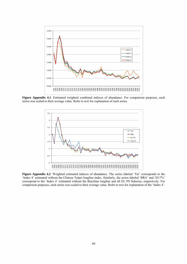
99

Figure Appendix 4.1. Estimated weighted combined indexes of abundance. For comparison purposes, each series was scaled to their average value. Refer to text for explanation of each series. Figure Appendix 4.2. Weighted estimated indexes of abundance. The series labeled ‘Tai’ corresponds to the ‘Index 4’ estimated without the Chinese Taipei longline index. Similarly, the series labeled ‘BRA’ and ‘EU7%’ correspond to the ‘Index 4’ estimated without the Brazilian longline and all EU PS fisheries, respectively. For comparison purposes, each series was scaled to their average value. Refer to text for explanation of the ‘Index 4’.

0

0.5

1

1.5

2

2.5

3

3.5

1965

1966

1967

1968

1969

1970

1971

1972

1973

1974

1975

1976

1977

1978

1979

1980

1981

1982

1983

1984

1985

1986

1987

1988

1989

1990

1991

1992

1993

1994

1995

1996

1997

1998

1999

2000

2001

2002

2003

2004

2005

2006

2007

2008

2009

2010

TAI

BRA

EC 7%

Index 4

0.000

0.500

1.000

1.500

2.000

2.500

3.000

3.500

1965

1966

1967

1968

1969

1970

1971

1972

1973

1974

1975

1976

1977

1978

1979

1980

1981

1982

1983

1984

1985

1986

1987

1988

1989

1990

1991

1992

1993

1994

1995

1996

1997

1998

1999

2000

2001

2002

2003

2004

2005

2006

2007

2008

2009

2010

Index 1

Index 2

Index 3

Index 4

100

Appendix 5

STANDARDIZATION OF THE CATCH RATES OF THE EUROPEAN

AND ASSOCIATED BAITBOAT FISHERY BASED IN DAKAR Response variable: Log (CPUE+0.1) Explanatory variables: Year=c(1969,1970,1971,1972,1973,1974,1975,1976,1977,1978,1979,1981,1982,1983,1984,1985,1986,1987, 1988,1989,1990,1991,1992,1993,1994,1995,1996,1997,1998,1999,2000,2001,2002,2003,2004,2005,2006, 2007,2008,2009,2010), Quarter=1:4, Fleet=c("MIXFIS","ESPETRO","FRAETRO","NEISEN")) ) Model Mtot<-glm(log(UYFT+0.1) ~ Year + Quarter + Fleet + Year:Quarter, family = gaussian) Model selection with library(MASS) Mtot.step<-stepAIC(Mtot) Mtot.step$anova (original model selected) Predicted values performed with an R Lsmeans procedure

Figure Appendix 5.1. Standardized CPUE for baitboats operating from Dakar.

0

1

2

3

4

5

6

7

8

9

10

1969

1971

1973

1975

1977

1979

1981

1983

1985

1987

1989

1991

1993

1995

1997

1999

2001

2003

2005

2007

2009

Stan

dardized CPUE ( t/ F. days )

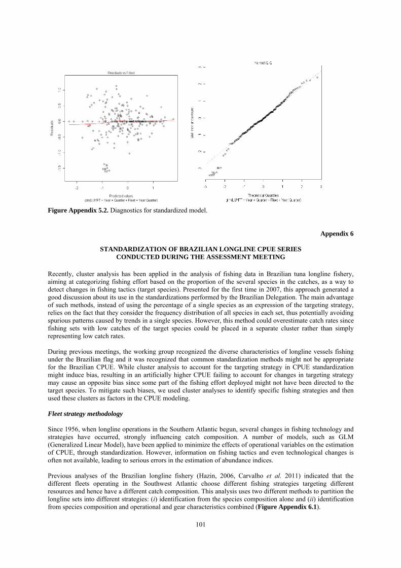
101

Figure Appendix 5.2. Diagnostics for standardized model.

Appendix 6

STANDARDIZATION OF BRAZILIAN LONGLINE CPUE SERIES CONDUCTED DURING THE ASSESSMENT MEETING

Recently, cluster analysis has been applied in the analysis of fishing data in Brazilian tuna longline fishery, aiming at categorizing fishing effort based on the proportion of the several species in the catches, as a way to detect changes in fishing tactics (target species). Presented for the first time in 2007, this approach generated a good discussion about its use in the standardizations performed by the Brazilian Delegation. The main advantage of such methods, instead of using the percentage of a single species as an expression of the targeting strategy, relies on the fact that they consider the frequency distribution of all species in each set, thus potentially avoiding spurious patterns caused by trends in a single species. However, this method could overestimate catch rates since fishing sets with low catches of the target species could be placed in a separate cluster rather than simply representing low catch rates. During previous meetings, the working group recognized the diverse characteristics of longline vessels fishing under the Brazilian flag and it was recognized that common standardization methods might not be appropriate for the Brazilian CPUE. While cluster analysis to account for the targeting strategy in CPUE standardization might induce bias, resulting in an artificially higher CPUE failing to account for changes in targeting strategy may cause an opposite bias since some part of the fishing effort deployed might not have been directed to the target species. To mitigate such biases, we used cluster analyses to identify specific fishing strategies and then used these clusters as factors in the CPUE modeling. Fleet strategy methodology Since 1956, when longline operations in the Southern Atlantic begun, several changes in fishing technology and strategies have occurred, strongly influencing catch composition. A number of models, such as GLM (Generalized Linear Model), have been applied to minimize the effects of operational variables on the estimation of CPUE, through standardization. However, information on fishing tactics and even technological changes is often not available, leading to serious errors in the estimation of abundance indices. Previous analyses of the Brazilian longline fishery (Hazin, 2006, Carvalho et al. 2011) indicated that the different fleets operating in the Southwest Atlantic choose different fishing strategies targeting different resources and hence have a different catch composition. This analysis uses two different methods to partition the longline sets into different strategies: (i) identification from the species composition alone and (ii) identification from species composition and operational and gear characteristics combined (Figure Appendix 6.1).

102

Two methods were used to determine fishing strategy. The first one, Fleet Strategy I, followed the clustering procedures described in Hazin et al. 2011. In the second method (Fleet Strategy 2) a matrix was constructed similar to the first method but now considering the seasonal (month) and operational factors (time fishing: night and day, boat length: <25m and >25m, hooks/basket: 3-6; 7-10; >10) using Multidimensional Scaling (MDS).

Figure Appendix 6.1 Method used to partition the longline sets into different strategies. Results and discussion

During the 2008 yellowfin tuna stock assessment meeting, the Brazilian CPUE series presented were estimated using the target species as a factor in the GLM. CPUE predictions were obtained for every year, fixing the level of remaining factors at the level with the highest number of observations. After years of discussion regarding the topic, now a consensus has been reached. The use of the current fleet-strategy factor in the Brazilian standardizations should be replaced A new standardized CPUE series was built using GLMM. Three data sets were used for standardized CPUE: all data; fleets with 5 years of operations and fleets with 7 years of operations. The initial analyses obtained predicted values for each observation and then took the mean of these for each year. After some discussion, the Group suggested that the estimates should be calculated by creating a balanced prediction matrix similar to the SAS lsmeans so that the estimates are not unduly influenced by the unbalanced data. Both standardized series showed a decline after the year 2000 (Figure Appendix 6.2) but the new estimated CPUE presented a significant difference from the previous one, most notable in the divergences from the nominal in the early years. In the future it is recommended to use a balanced prediction matrix to calculate the year effect in a balanced manner.

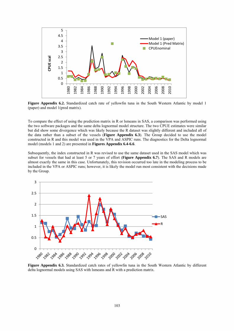
103

Figure Appendix 6.2. Standardized catch rate of yellowfin tuna in the South Western Atlantic by model 1 (paper) and model 1(pred matrix).

To compare the effect of using the prediction matrix in R or lsmeans in SAS, a comparison was performed using the two software packages and the same delta lognormal model structure. The two CPUE estimates were similar but did show some divergence which was likely because the R dataset was slightly different and included all of the data rather than a subset of the vessels (Figure Appendix 6.3). The Group decided to use the model constructed in R and this model was used in the VPA and ASPIC runs. The diagnostics for the Delta lognormal model (models 1 and 2) are presented in Figures Appendix 6.4-6.6. Subsequently, the index constructed in R was revised to use the same dataset used in the SAS model which was subset for vessels that had at least 5 or 7 years of effort (Figure Appendix 6.7). The SAS and R models are almost exactly the same in this case. Unfortunately, this revision occurred too late in the modeling process to be included in the VPA or ASPIC runs; however, it is likely the model run most consistent with the decisions made by the Group.

Figure Appendix 6.3. Standardized catch rates of yellowfin tuna in the South Western Atlantic by different delta lognormal models using SAS with lsmeans and R with a prediction matrix.

00.51

1.52

2.53

3.54

4.55

1980

1982

1984

1986

1988

1990

1992

1994

1996

1998

2000

2002

2004

2006

2008

2010

CPUE scal

Model 1 (paper)Model 1 (Pred Matrix)CPUEnominal

0

0.5

1

1.5

2

2.5

3

SAS

R

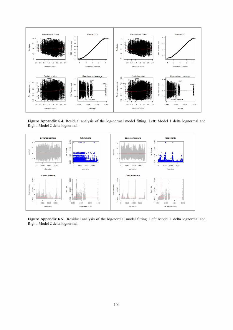
104

Figure Appendix 6.4. Residual analysis of the log-normal model fitting. Left: Model 1 delta lognormal and Right: Model 2 delta lognormal.

Figure Appendix 6.5. Residual analysis of the log-normal model fitting. Left: Model 1 delta lognormal and Right: Model 2 delta lognormal.

105

Figure Appendix 6.6. Plot standardized deviance residuals and explanatory variable of the linear predictor. Left: Model 1 delta lognormal and Right: Model 2 delta lognormal.

Figure Appendix 6.7. Standardized catch rate of yellowfin tuna in the South Western Atlantic revised to include only vessels with either a 5 or 7 year history.

Appendix 7

CHANGES IN FISHING POWER OF THE TROPICAL PURSE SEINE FLEET

Background Many studies have reported that changes in technology and fishing strategy of the tropical tuna purse seine fleets have led to significant changes in capacity and fishing power of individual vessels (Gaertner and Sachi 2000, Suzuki et al 2003, Joseph 2005 ). Few studies, however, have estimated the magnitude of these changes for the entire fleet and calculated the increased catchability of tuna resulting from such fishing power increases. Gascuel et al (1993) estimated increases of 17% per year and 9% per year for the period of 1980-1990 for the French fleet and the Spanish fleet, respectively by using a VPA. Reid et al (2005) estimated with the data

0

0.5

1

1.5

2

2.5

3

3.5

4

1980

1982

1984

1986

1988

1990

1992

1994

1996

1998

2000

2002

2004

2006

2008

2010

Delta‐log‐R (refit) Delta‐log‐SAS (Refit)

CPUEn uper

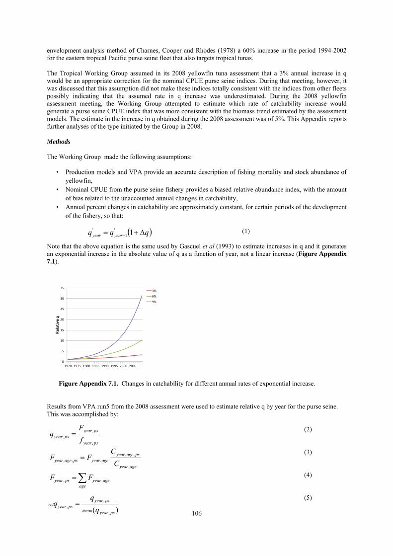
106

0

5

10

15

20

25

30

35

1970 1975 1980 1985 1990 1995 2000 2005

Relative q

3%

6%

9%

envelopment analysis method of Charnes, Cooper and Rhodes (1978) a 60% increase in the period 1994-2002 for the eastern tropical Pacific purse seine fleet that also targets tropical tunas. The Tropical Working Group assumed in its 2008 yellowfin tuna assessment that a 3% annual increase in q would be an appropriate correction for the nominal CPUE purse seine indices. During that meeting, however, it was discussed that this assumption did not make these indices totally consistent with the indices from other fleets possibly indicating that the assumed rate in q increase was underestimated. During the 2008 yellowfin assessment meeting, the Working Group attempted to estimate which rate of catchability increase would generate a purse seine CPUE index that was more consistent with the biomass trend estimated by the assessment models. The estimate in the increase in q obtained during the 2008 assessment was of 5%. This Appendix reports further analyses of the type initiated by the Group in 2008. Methods The Working Group made the following assumptions: • Production models and VPA provide an accurate description of fishing mortality and stock abundance of

yellowfin, • Nominal CPUE from the purse seine fishery provides a biased relative abundance index, with the amount

of bias related to the unaccounted annual changes in catchability, • Annual percent changes in catchability are approximately constant, for certain periods of the development

of the fishery, so that:

(1) Note that the above equation is the same used by Gascuel et al (1993) to estimate increases in q and it generates an exponential increase in the absolute value of q as a function of year, not a linear increase (Figure Appendix 7.1).

Figure Appendix 7.1. Changes in catchability for different annual rates of exponential increase.

Results from VPA run5 from the 2008 assessment were used to estimate relative q by year for the purse seine. This was accomplished by: (2) (3) (4) (5)

psyear

psyearpsyear f

Fq

,

,,

ageageyearpsyear

ageyear

psageyearageyearpsageyear

FF

C

CFF

,,

,

,,,,,

)( ,

,,

psyearmean

psyearpsyearrel

q

qq

qqq yearyear 1'1

'

107

Where nominal fishing effort (fishing days) in the purse seine for a given year relative catchability of the purse seine scaled to its mean for a given year fishing mortality produced by the purse seine in a given year for all age groups catch of the purse seine for a given year for all age groups fishing mortality by the purse seine in a given year for a given age catch of the purse seine in a given year for a given year Similarly relative catchability of the purse seine was calculated from production model estimates of biomass obtained in (2008) by using a logistic production model with MSY = 150,000, BMSY = 237,131 and B1949 = K = 644,588. These parameters represent approximately case 08 from the 2008 yellwofin assessment. (6) (7) (8) Where,

is the estimated biomass by the production model for a given year which corresponds to the biomass at the end of the calendar year, and

is the average biomass during the year. The relative catchability for the purse seine from a given year was then calculated from equation (1), as it was the case for the VPA results. Note that in the production model case, estimates of F and B were partially conditioned by the assumption made in 2008 that the annual increase in q for the purse seine was of 3%. Estimates of q obtained from the VPA were partially conditioned by the same assumption but only for the period 1970-because for the later period the free school and FAD indices were used and those indices were not corrected by an annual increase in q. Although it would be best to have used estimates of q not conditioned by the old assumption of the 3% annual rate of increase in q such estimates were not available. It is hoped that given that in both the production model and the VPA implementations conducted in 2008 purse seine indices did not fit the models well that those indices were not very influential in the model fit and the final estimates of biomass and fishing mortality. Once the two sets of relative q were estimated, one from the VPA and one from the production model, the data were broken up into three periods where it was assumed that there would be a constant annual increase in q. The first period corresponded to the period prior to substantial development of the FAD fishery 1970-1989; the second the period of fast development of the FAD fishery 1990-1999 and the third the most recent period 2000-2006. A single was estimated for each period by minimizing the joined sum of squares:

′ ′

Where ′ was calculated from equation (1) for each period. It was assumed that the q calculated for the end of each period was the q for the beginning of the next period. As a result only two additional nuisance

periodq

psyearrelq ,

psyearC ,

psyearF ,

psageyearF ,,

psageyearC ,,

2

_ 1

_

,,

yearyear

year

yearyear

year

psyearyearpsyear

BB

CF

C

CFF

B

B year

yearB

yearB_

psyearf ,

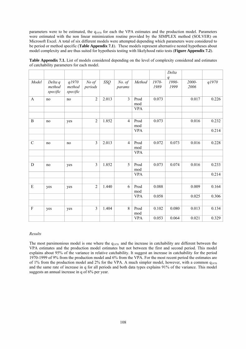
108

parameters were to be estimated, the q1970 for each the VPA estimates and the production model. Parameters were estimated with the non linear minimization routine provided by the SIMPLEX method (SOLVER) on Microsoft Excel. A total of six different models were attempted depending which parameters were considered to be period or method specific (Table Appendix 7.1). These models represent alternative nested hypotheses about model complexity and are thus suited for hypothesis testing with likelyhood ratio tests (Figure Appendix 7.2). Table Appendix 7.1. List of models considered depending on the level of complexity considered and estimates of catchability parameters for each model.

Delta q

Model Delta q method specific

q1970 method specific

No of periods

SSQ No. of params

Method 1970-1989

1990-1999

2000-2006

q1970

A no no 2 2.013 3 Prod mod

0.073 0.017 0.226

VPA

B no yes 2 1.852 4 Prod mod

0.073 0.016 0.232

VPA 0.214

C no no 3 2.013 4 Prod mod

0.072 0.073 0.016 0.228

VPA

D no yes 3 1.852 5 Prod mod

0.073 0.074 0.016 0.233

VPA 0.214

E yes yes 2 1.440 6 Prod mod

0.088 0.009 0.164

VPA 0.058 0.025 0.306

F yes yes 3 1.404 8 Prod mod

0.102 0.080 0.013 0.134

VPA 0.053 0.064 0.021 0.329

Results The most parsimonious model is one where the q1970 and the increase in catchability are different between the VPA estimates and the production model estimates but not between the first and second period. This model explains about 95% of the variance in relative catchability. It suggest an increase in catchability for the period 1970-1999 of 9% from the production model and 6% from the VPA. For the most recent period the estimates are of 1% from the production model and 2% for the VPA. A much simpler model, however, with a common q1970

and the same rate of increase in q for all periods and both data types explains 91% of the variance. This model suggests an annual increase in q of 6% per year.

109

A

B

D

C

E

3

Number of parameters

4

5

6

F 8

Figure Appendix 7.2. Schematic representation of the complexity and nested relationship between different models considered. Table Appendix 7.2. Likelihood ratio test for competing models in Table Appendix 7.1.

Likehood ratio tests

Increase in variance explained

(%) df x2 p

A vs B 1 4.36 0.037 0.55

A vs C 1 0.00 0.946 0.00

B vs D 1 0.00 0.976 0.00

C vs D 1 4.35 0.037 0.55

B vs E 2 13.07 0.001 1.40

E vs F 2 1.31 0.520 0.12 C vs F 4 18.73 0.001 2.07 A vs F 5 18.74 0.002 2.07 A vs E 3 17.43 0.001 1.95 B vs E 2 13.07 0.001 1.40

110

Figure Appendix 7.3. Estimates of annual relative catchability of purse seine from VPA (diamonds) and production models (squares). Fit corresponds to model B with a rate of annual increase of 7% for the period 1970-1999 and 1.5% from 2000 to 2006. Discussion Our estimates of annual increase in fishing power are similar to the 6% annual rates obtained by Reid et al (2005) for the purse seine fleet of the tropical eastern Pacific and much lower than the rates obtained by Gascuel et al in 1993. Both of these studies were conducted over a smaller range of years, and we do not discount that at certain periods the rate of increase may be greater than the average rate calculated herein. In addition, the study of Gascuel et al (1993) acknowledge that part of the gains in efficiency estimated in their study relate to the area fished, which tipically are not considered by other studies and are certainly not part of the non-spatially structured models used in the assessment of Atlantic yellowfin tuna. Finally, the study of Gascuel et al (1993) was conducted at a time where the data for 1980-1990 were recently obtained and it has been shown repeatedly in yellowfin assessment that the most recent estimates of biomass and fishing mortality from VPA suffer from retrospective trends, thus such estimates are less reliable than those obtained at a later time when more data have accumulated Given that the purpose of this analysis was to determine period specific estimates of change in catchability, the Working Group decided to use the results from model B which explains 94% of the variance (Figure Appendix 7.3). This model suggests that the annual rate of increase in q was 7% from 1970 to 1999 and has been at about 1.5% from 2000-2006. References Charnes, A., Cooper, W.W. and Rhodes, E. 1978, Measuring the efficiency of decision making units. European

Journal of Operational Research, 2: 429-444.

Gaertner, D. and Sacchi, J. 2000, Changes over time in net dimensions in French tropical purse seiners operating in the Atlantic Ocean. Collect. Vol. Sci. Pap. ICCAT, 51(2): 571-580.

Gascuel, D., Fonteneau, A. and Foucher, E. 1993, Analyse de l'évolution des puissances de pêche par l'analyse des cohortes: application aux senneurs exploitant l'albacore (Thunnus albacares) dans l'Atlantique Est. Aquatic Living Resources, 6(1): pp.15-30.

0

0.5

1

1.5

2

2.5

3

1970 1975 1980 1985 1990 1995 2000 2005

relative

catchability (q)

q estimates

q VPA

q production model

q pred VPA

q pred Prod Mod

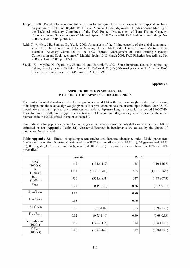
111

Joseph, J. 2005, Past developments and future options for managing tuna fishing capacity, with special emphasis on purse-seine fleets. In: Bayliff, W.H., Leiva Moreno, J.I. de, Majkowski, J. (eds.) Second Meeting of the Technical Advisory Committee of the FAO Project “Management of Tuna Fishing Capacity: Conservation and Socio-economics”. Madrid, Spain, 15-18 March 2004. FAO Fisheries Proceedings. No. 2. Rome, FAO. 2005. p 281-323.

Reid, C., Kirkley, J.E., Squires, D., Ye, J. 2005, An analysis of the fishing capacity of the global tuna purse-seine fleet. In: Bayliff, W.H.;,Leiva Moreno, J.I. de, Majkowski, J. (eds.) Second Meeting of the Technical Advisory Committee of the FAO Project “Management of Tuna Fishing Capacity: Conservation and Socio-economics”. Madrid, Spain, 15-18 March 2004. FAO Fisheries Proceedings. No. 2. Rome, FAO. 2005. pp 117- 157.

Suzuki, Z., Miyabe, N., Ogura, M., Shono, H. and Uozumi, Y. 2003, Some important factors in controlling fishing capacity in tuna fisheries Pascoe, S., Gréboval, D. (eds.) Measuring capacity in fisheries. FAO Fisheries Technical Paper. No. 445. Rome, FAO. p 91-98.

Appendix 8

ASPIC PRODUCTION MODELS RUN WITH ONLY THE JAPANESE LONGLINE INDEX

The most influential abundance index for the production model fit is the Japanese longline index, both because of its length, and the relative high weight given to it in production models that use multiple indices. Four ASPIC models were run with updated catch estimates and updated Japanese longline index for the period 1965-2010. These four models differ in the type of production model function used (logistic or generalized) and in the initial biomass ratio in 1950/K (fixed to one or estimated)). Point estimates for population parameters are very similar between runs that only differ on whether the B1/K is estimated or not (Appendix Table 8.1). Greater differences in benchmarks are caused by the choice of production function used. Table Appendix 8.1. Effects of updating recent catches and Japanese abundance index. Model parameters (median estimates from bootstraps) estimated by ASPIC for runs 01 (logistic, B1/K =1), 02 (generalized, B1/K =1), 03 (logistic, B1/K =est.) and 04 (generalized, B1/K =est.). In parenthesis are shown the 10% and 90% percentiles.)

Run 01 Run 02

MSY (1000s t)

142 (131.6-149) 135 (110-136.7)

K (1000s t)

1051 (703.8-1,703) 1505 (1,401-3162.)

BMSY (1000s t)

526 (351.9-851) 527 (448-807.9)

FMSY

0.27 0.15-0.42) 0.26 (0.15-0.31)

B2006/BMSY

1.15 0.80

F2006/FMSY

0.63 0.96

B2010/BMSY

0.86 (0.7-1.02) 1.03 (0.92-1.21)

F2010/FMSY

0.92 (0.75-1.16) 0.80 (0.68-0.93)

Y equilibrium (1000s t)

140 (122.2-148) 112 (108-113.1)

Y FMSY (1000s t)

140 (122.2-148) 112 (108-113.1)

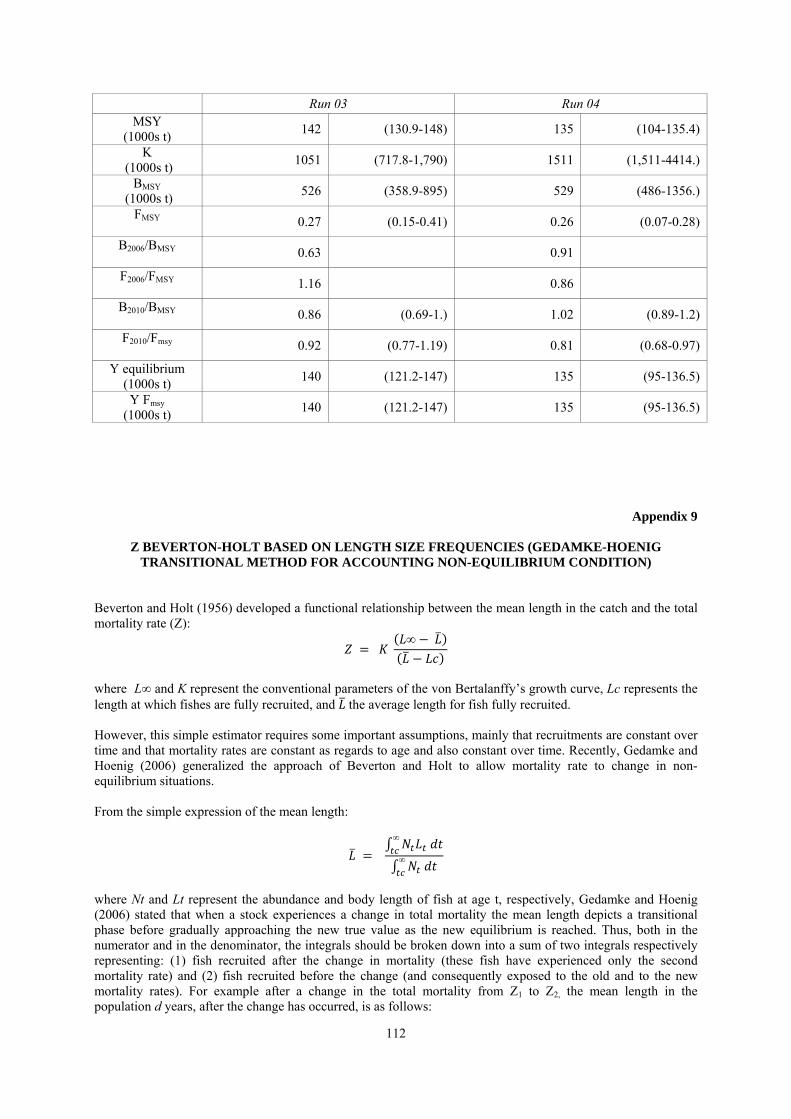
112

Run 03 Run 04 MSY

(1000s t) 142 (130.9-148) 135 (104-135.4)

K (1000s t)

1051 (717.8-1,790) 1511 (1,511-4414.)

BMSY (1000s t)

526 (358.9-895) 529 (486-1356.)

FMSY

0.27 (0.15-0.41) 0.26 (0.07-0.28)

B2006/BMSY

0.63 0.91

F2006/FMSY

1.16 0.86

B2010/BMSY

0.86 (0.69-1.) 1.02 (0.89-1.2)

F2010/Fmsy

0.92 (0.77-1.19) 0.81 (0.68-0.97)

Y equilibrium (1000s t)

140 (121.2-147) 135 (95-136.5)

Y Fmsy (1000s t)

140 (121.2-147) 135 (95-136.5)

Appendix 9

Z BEVERTON-HOLT BASED ON LENGTH SIZE FREQUENCIES (GEDAMKE-HOENIG

TRANSITIONAL METHOD FOR ACCOUNTING NON-EQUILIBRIUM CONDITION) Beverton and Holt (1956) developed a functional relationship between the mean length in the catch and the total mortality rate (Z):

∞

where L∞ and K represent the conventional parameters of the von Bertalanffy’s growth curve, Lc represents the length at which fishes are fully recruited, and the average length for fish fully recruited.

However, this simple estimator requires some important assumptions, mainly that recruitments are constant over time and that mortality rates are constant as regards to age and also constant over time. Recently, Gedamke and Hoenig (2006) generalized the approach of Beverton and Holt to allow mortality rate to change in non-equilibrium situations. From the simple expression of the mean length:

∞

∞

where Nt and Lt represent the abundance and body length of fish at age t, respectively, Gedamke and Hoenig (2006) stated that when a stock experiences a change in total mortality the mean length depicts a transitional phase before gradually approaching the new true value as the new equilibrium is reached. Thus, both in the numerator and in the denominator, the integrals should be broken down into a sum of two integrals respectively representing: (1) fish recruited after the change in mortality (these fish have experienced only the second mortality rate) and (2) fish recruited before the change (and consequently exposed to the old and to the new mortality rates). For example after a change in the total mortality from Z1 to Z2, the mean length in the population d years, after the change has occurred, is as follows:

113

∞

∞

(for a general expression for the mean length after multiple changes in the mortality rate, see Appendix 2 in Gedamke and Hoenig, 2006). Therefore, given a series of annual observations of mean length over time it is possible to estimate the original total mortality rate, the year in which it changed and the new mortality rate (possibly even the next breaking date and resulting change in mortality rate, etc.). To assess whether there have been multiple changes in the mortality rates of yellowfin, different competing models (i.e., with different breaking dates and resulting number of parameters) were ranked according to the Akaike information criterion. The top-ranking model (i.e., smallest AIC) from this set was reported as the most parsimonious model, which is the model that best explains the variation in the data while using the fewest parameters. Results N. breaks N. par. AIC Breaking dates

2 6 523.36 1979, 1996 3 8 533.11 1979-1980, 1996, 2005 1 4 536.01 1994 4 10 621.64 1979, 1984, 1995-1996, 2005 Model selection for determining mortality rates from mean length data in non-equilibrium situations for Atlantic yellowfin (1970-2010), with (N. breaks) number of change points in total mortality, (N. par.) number of parameters, (AIC) Akaike Information Criterion and breaking dates Parameter Estimate SE t

Z1 1.081 0.063 17.14 Z2 1.519 0.057 26.67 Z3 2.429 0.123 19.76 Y1 1978.623 0.655 14.69 Y2 1996.052 0.590 45.85 SD 310.044 34.267 9.05 Summary statistics for the best model estimating mortality from mean length data in non-equilibrium situations for Atlantic yellowfin (1970-2010) when three different levels of mortality and two years of change are estimated simultaneously. Reference Gedamke, T. and Hoenig, J. M. 2006, Estimating mortality from mean length data in non-equilibrium situations,

with application to the assessment of goosefish. Trans. Am fish. Soc. 135: 476-487.

REPORT OF THE 2011 ICCAT YELLOWFIN TUNA STOCK ASSESSMENT ... · REPORT OF THE 2011 ICCAT YELLOWFIN...

Documents

Transcript of REPORT OF THE 2011 ICCAT YELLOWFIN TUNA STOCK ASSESSMENT ... · REPORT OF THE 2011 ICCAT YELLOWFIN...