Stochastic gradient variational Bayes for gamma ...
14
Stochastic gradient variational Bayes for gamma approximating distributions David A. Knowles Stanford University [email protected] September 8, 2015 Abstract While stochastic variational inference is relatively well known for scal- ing inference in Bayesian probabilistic models, related methods also offer ways to circumnavigate the approximation of analytically intractable ex- pectations. The key challenge in either setting is controlling the variance of gradient estimates: recent work has shown that for continuous latent variables, particularly multivariate Gaussians, this can be achieved by us- ing the gradient of the log posterior. In this paper we apply the same idea to gamma distributed latent variables given gamma variational distribu- tions, enabling straightforward “black box” variational inference in models where sparsity and non-negativity are appropriate. We demonstrate the method on a recently proposed gamma process model for network data, as well as a novel sparse factor analysis. We outperform generic sampling algorithms and the approach of using Gaussian variational distributions on transformed variables. 1 Introduction Bayesian probabilistic models offer a clean, interpretable methodology for ap- plied statistical analysis. However, inference remains a challenge both in terms of ease of implementation and scalability. Ease of implementation is important so that practitioners can construct models tailored specifically to their applica- tion, rather than being forced to choose from a small set of pre-existing models. While various software packages, such as Infer.NET (Minka et al., 2010), Win- BUGS (Lunn et al., 2000), Church (Goodman et al., 2012) and more recently, STAN (Stan Development Team, 2014), have been designed explicitly to address this problem, they do not currently scale to large real world datasets. Stochastic variational inference (SVI) methods (Hoffman et al., 2010, 2013), follow the traditional variational Bayes approach of converting an intractable integration into a optimization problem. However, where VB would usually proceed by the well known coordinate ascent updates on the variational lower 1 arXiv:1509.01631v1 [stat.ML] 4 Sep 2015
Transcript of Stochastic gradient variational Bayes for gamma ...
Stochastic gradient variational Bayes for gamma
approximating distributions
David A. KnowlesStanford [email protected]
September 8, 2015
Abstract
While stochastic variational inference is relatively well known for scal-ing inference in Bayesian probabilistic models, related methods also offerways to circumnavigate the approximation of analytically intractable ex-pectations. The key challenge in either setting is controlling the varianceof gradient estimates: recent work has shown that for continuous latentvariables, particularly multivariate Gaussians, this can be achieved by us-ing the gradient of the log posterior. In this paper we apply the same ideato gamma distributed latent variables given gamma variational distribu-tions, enabling straightforward “black box” variational inference in modelswhere sparsity and non-negativity are appropriate. We demonstrate themethod on a recently proposed gamma process model for network data,as well as a novel sparse factor analysis. We outperform generic samplingalgorithms and the approach of using Gaussian variational distributionson transformed variables.
1 Introduction
Bayesian probabilistic models offer a clean, interpretable methodology for ap-plied statistical analysis. However, inference remains a challenge both in termsof ease of implementation and scalability. Ease of implementation is importantso that practitioners can construct models tailored specifically to their applica-tion, rather than being forced to choose from a small set of pre-existing models.While various software packages, such as Infer.NET (Minka et al., 2010), Win-BUGS (Lunn et al., 2000), Church (Goodman et al., 2012) and more recently,STAN (Stan Development Team, 2014), have been designed explicitly to addressthis problem, they do not currently scale to large real world datasets.
Stochastic variational inference (SVI) methods (Hoffman et al., 2010, 2013),follow the traditional variational Bayes approach of converting an intractableintegration into a optimization problem. However, where VB would usuallyproceed by the well known coordinate ascent updates on the variational lower
1
arX
iv:1
509.
0163
1v1
[st
at.M
L]
4 S
ep 2
015

bound (Jordan et al., 1999), SVI utilizes the key idea of stochastic gradientdescent: that it is enough to follow noisy, but unbiased, estimates of the gradient(Robbins & Monro, 1951). If these noisy gradients can be computed much morecheaply than full gradients, e.g. by subsampling the data, then more rapidconvergence is typically possible and the volume of data which can be handledis greatly increased.
The observation that noisy, unbiased gradients can be used in variationalinference suggests another idea: instead of analytically calculating the requiredexpectations and gradient of the lower bound can we just use Monte Carlo?The challenge in applying this idea is to keep the variance of the Monte Carlogradient estimates low without requiring a computationally infeasible number ofsamples. Various “tricks” have been proposed to achieve this, including controlvariates (Paisley et al., 2012), stochastic linear regression (Salimans & Knowles,2013) and using the factor graph structure of the model (Ranganath et al.,2013). We focus on a recently proposed solution for continuous latent variablesproposed independently by Salimans & Knowles (2013) and Kingma & Welling(2013) which utilizes just the gradient of the log posterior, which we refer to asstochastic gradient variational Bayes (SGVB). While both papers demonstratedthe effectiveness of this approach for multivariate Gaussian variables, whetherit is equally useful for latent variables with very different distributions remainsan open question. In this paper we investigate using gamma approximatingdistributions. Compared to the Gaussian case, gamma r.v.s represent a naturalstep in the direction of more structured models: despite being continuous theycan encode sparsity using suitably small shape parameters, while also enforcingnon-negativity, which is appropriate in many settings. In addition gamma r.v.salso underly many of the most commonly used Bayesian nonparametric priorssuch as the Dirichlet process.
The variational autoencoder Kingma & Welling (2013) uses a variationalinference methodology where the approximate posterior is a function, knownas the recognition model, of the observed data. This allows extremely scalabletraining using stochastic gradient descent analogously to a standard autoen-coder. While having certain advantages, this approach can be sensitive to thechoice of recognition model, has only been demonstrated for Gaussian latentvariables, does not straightforwardly handle missingness in the observations andonly performs MLE over the model parameters.
Related methodology has very recently been incorporated into Stan (Ku-cukelbir et al., 2015). Their approach is to always use a fully factorized Gaus-sian variational posterior but to reparameterize such that the space of the r.v.sis always the reals. For r.v.s constrained to be positive for example, this cor-responds to using a log-normal variational posterior. Our experiments heresuggest that explicitly using gamma variational posteriors, at least when thepriors are gamma, is preferable.
In Section 2 we review stochastic gradient variational Bayes (SGVB), showhow to leverage the gradient wrt to the log joint and present the necessaryderivations for gamma r.v.s. We present two models in Section 3 which we useas test cases. The first is the infinite edge partition model (Zhou, 2015) for
2
network data, the second a novel gamma process factor analysis model (GPFA)for arbitrary continuous data. In Section 4 we present promising results for bothmodels on synthetic and real world data and conclude in Section 5 with somepotential future directions.
2 Methods
In this section we review variational inference, show how the required gradientscan be approximated using Monte Carlo and then turn to the particular case ofgamma r.v.s.
2.1 Variational inference
Let the normalized distribution of interest be p(x) = f(x)/Z. Typically p isthe posterior, f is the joint and Z is the marginal likelihood (evidence). We useJensen’s inequality to lower bound
logZ = log
∫x
f(x)dx = log
∫x
q(x)f(x)
q(x)dx ≥
∫x
q(x) logf(x)
q(x)dx =: F [q]. (1)
where q represents the variational posterior. We can ask what error we aremaking between the true Z and the Evidence Lower BOund (ELBO) F [q]:
logZ −F [q] =
∫x
q(x) logq(x)
p(x)dx =: KL(q||p) = −H[q(x)]−
∫q(x) log p(x)dx,
(2)
where KL(q||p) is the KL divergence and H[q(x)] = −∫q(x) log q(x)dx is the
entropy. In general we can evaluate F [q] but not the KL itself, since this wouldrequire knowing Z. By maximising the lower bound F [q] we will minimize theKL divergence. The KL divergence is strictly positive for q 6= p and equal to0 only for q = p. As a result finding the general q which minimizes the KLdivergence is no easier than the original inference task, which we assume isintractable. The usual strategy therefore is to place simplifying constraints onq, the most popular, due to its simplicity, being the mean field approximation.We will take the approach of choosing q to have a specific parametric form,indexed by θ. Typically qθ will be in the exponential family: in this paper inparticular, qθ will be a product of gamma distributions.
2.2 SGVB for continuous latent variables
To fit qθ we will maximize F [qθ] wrt to θ, which requires estimating the gradient
∇θF [qθ] = ∇θEqθ [log f(x)− log qθ(x)] (3)
This form is not easily amenable to Monte Carlo estimation because of thedependence of qθ on θ. One approach is to use the identity ∇θEqθ [L(x)] =
3

Eqθ [L(x)∇θ log qθ(x)] where L(x) = log f(x) − log qθ(x), but this typically hashigh variance. Instead, assume we can find a random variable z ∼ π(z) suchthat x = ψ(z, θ) has the same distribution as x ∼ qθ, then
∇θEqθ [L(x)] = Eπ(z)[∇θψ(z, θ)∇xL(f(z, θ))]. (4)
Since π(z) has no dependence on θ the RHS expression is straightforward toapproximate by Monte Carlo,
∇θEqθ [L(x)] ≈ 1
S
S∑s=1
∇θψ(z(s), θ)∇xL(x(s)), where z(s) ∼ π,x(s) = ψ(z(s), θ).
In fact, this estimator generally has low enough variance that we can simply useS = 1.
For Gaussian random variables x an obvious choice is π(z) = N(0, I) and
ψ(z, {m,V}) = m+V12 z where {m,V} are the mean and (co)variance respec-
tively. For gamma random variables no such simple transformation exists, sowe resort to the generic CDF transform instead. For any random variable xwith CDF Fθ(x) we can sample x as
z ∼ U [0, 1], x = F−1θ (z) =: ψ(z, θ) (5)
where U [0, 1] is the uniform distribution on [0, 1]. We can differentiate ψ(z, θ)with respect to θ as
∇θψ(z, θ) = −∇θFθ(x)
fθ(x)(6)
where fθ(x) is the pdf of x.
2.3 Gamma variational distributions
For a gamma latent variable with shape a and rate b
Fa,b(x) =
∫ x
0
ba
Γ(a)ta−1e−btdt. (7)
It is straightforward to differentiate this expression wrt b and use Equation 6to obtain ∇bψ(z, a, b). However the result is easier to obtain by noting thatx = F−1
a,b (z) = F−1a,1 (z)/b and so
∇bψ(z, a, b) = ∇bF−1a,b (z) = ∇bF−1
a,1 (z)/b = −F−1a,1 (z)/b2 = −x/b (8)
Unfortunately the gradient wrt to the shape a has no analytical form in termsof commonly available special functions. Depending on the order of magnitudeof a different approaches can be used to accurately and efficiently approximate∇aψ(z, a, b). For moderate values of a we use a finite difference approximation
∇aF−1a,b (z) ≈
F−1a+ε,b(z)− F
−1a,b (z)
ε, (9)
4
where ε is a small positive constant. We use of the high numerical precisionof the gaminv Matlab function (the Boost C++ library also implements such afunction), which calculates F−1 using an iterative solver.
For small values of a � 1 gaminv often fails to converge. This regime isimportant because it corresponds to the gamma distribution’s ability to modelsparsity. Fortunately, in this regime the asymptotic approximation Fa,1(x) ≈xa
aΓ(a) becomes increasingly accurate, so that
F−1a,b (z) ≈ (zaΓ(a))
1a /b (10)
For a < 1 and (1−0.94z) log(a) < −0.42 we use Equation 10 to efficiently obtainboth x and ∇aψ(z, a, b) without expensive calls to gaminv, whilst keeping theabsolute relative error below 10−4. Finally for large a � 1 (we use a > 1000)the gamma distribution is well approximated by a Gaussian with matched meanand variance, i.e. ψ(z′, a, b) ≈ (a +
√az′)/b and ∇aψ(z′, a, b) ≈ (1 + z′/
√a)/b
where z′ ∼ N(0, 1).
2.4 Optimization
The shape and rate parameters for the gamma distribution are of course re-quired to be positive. To cope with this we use the reparameterisation r(θ) =log(1 + exp (θ)) for both the shape and rate to avoid performing constrainedoptimisation. Pseudocode is shown in Algorithm 1 for the basic algorithm. Wealso experimented with incorporating momentum, and using AdaGrad (Duchiet al., 2011), RMSprop (Tieleman & Hinton, 2012) or AdaDelta (Zeiler, 2012)to set the learning rate. Momentum involves maintaining an additional velocityvector v which is updated as v ← λg + (1 − λ)v where g is the gradient andλ ∈ [0, 1] is the momentum parameter. v is then used in the place of g whenupdating the parameters. Our implementation of AdaGrad uses a step-size
γ(t) = 0.1/(
10−6 +√∑t
j=1 g2t
)where gt is the gradient at step t. RMSprop is
similar in spirit to AdaGrad: we maintain a running average m← 0.1g2 +0.9m,and use a step-size γ(t) = 0.01/
(1× 10⁻⁶ +
√m). AdaDelta is a heuristic which
tries to maintain progress in later stages of the optimization by keeping the samerunning average of squared gradients as RMSprop, mg ← ρg2 + (1−ρ)mg (withρ ∈ [0, 1]), as well as mθ ← ρ(∆θ)2 + (1 − ρ)mθ (where ∆θ is the update inparameter space), and using a step-size γ =
√(mθ + ε)/
√(mg + ε), where we
use ε = 10−4.
3 Models
In this section we briefly outline the models we will use to assess the algorithm.We choose models which only involve gamma latent variables, but emphasizethat models involving both Gaussian and gamma latent variables would also bestraightforward to implement.
5
Algorithm 1 Gamma stochastic gradient variational Bayes
Initialize t = 0, a,b.α = r−1(a),β = r−1(b)repeat
Sample zd ∼ U [0, 1]Set xd = F−1
ad,bd(zd) according to Section 2.3
Set g = ∇x[log f(x)− log qa,b(x)]Set gαd = gd∇aF−1
ad,bd(zd)/(1 + e−αd)
Set gβd = gd∇bF−1ad,bd
(zd)/(1 + e−βd)
Compute step size γ(t) (e.g. using AdaDelta on [gα, gβ ]))αd ← αd + γ(t)gα
βd ← βd + γ(t)gβ
a = r(α),b = r(β)t := t+ 1
until convergence
3.1 Infinite edge partition model
There has been considerable recent interest in probabilistic modelling of net-work data, typically represented as an undirected graph (Kemp & Tenenbaum,2006; Blundell & Teh, 2013),. In a social network nodes will represent individ-uals and edges friendships, or in a protein interaction network nodes representproteins and edges physical interaction. Let Y ∈ {0, 1}N×N represent the bi-nary adjacency matrix of the graph: yij = yji indicates whether there is a linkbetween nodes i and j. Many models have been proposed to uncover the latentstructure in such data, but we will focus on the recent infinite edge partitionmodel (EPM, Zhou, 2015), which specifies
P (yij = 1|W ) = 1− exp
(−∑k
rkwikwjk
)(11)
where W is a N × K matrix of positive reals and r is a K-vector of re-als. This link function can be interpreted as summing over latent variablessijk ∼ Poisson(rkwikwjk) and taking yij = I[0 <
∑Kk=1 sijk]. This link func-
tion has two advantages over logistic link functions: i) it is appropriate forsparse graphs since P (yij = 1|W ) is small when W ≈ 0, ii) the correspondinglikelihood can be evaluated with computational cost linear in the number ofobserved present and missing edges (as noted by Morup et al. (2011)), whichis typically orders of magnitude smaller than N2. To see this note that thelikelihood is∑
i>j
Mij [Yij log (1− e−pij ) + (1− Yij)(−pij)]
=∑i>j
MijYij [log (1− e−pij ) + pij ] +∑i>j
(1−Mij)pij −∑i>j
pij (12)
6
where Mij = 1 iff edge ij is not missing and 0 o.w., and pij =∑k wikwjk. The
first sum only involves non-missing existing edges, the second sum only missingedges, and the third sum can be calculated efficiently in O(NK) as∑
i>j
pij =∑i>j
∑k
wikwjk =1
2
∑k
[w2·k −
∑i
w2ik] (13)
where w·k =∑i wik.
To complete the prior specification we use
Wik|ai, ci ∼ G(ai, ci), ai ∼ G(0.01, 0.01), ci ∼ G(1, 1),
rk|γ0, c0 ∼ G(γ0/K, c0), γ0 ∼ G(1, 1), c0 ∼ G(1, 1) (14)
where the distribution on rk is a finite K approximation to the gamma process.
3.2 Gamma process factor analysis
Factor analysis models are appealing for finding latent structure in high dimen-sional data. Observed data samples yn ∈ RD, n = 1 . . . N are modeled as
yn|xn ∼ N(Wxn, σ2I) (15)
where typically xn ∼ N(0, I). Many approaches exist to fitting such models.From a Bayesian viewpoint, if W is given a Gaussian prior then Gibbs sam-pling x|W,− and W |x,− is straightforward and conjugate, although even inthis simple setting the strong posterior dependencies between x and W can beproblematic for convergence and mixing. We consider placing a Gamma prioron the elements of W , thereby enforcing positivity. Such “semi”-nonnegativematrix factorization (NMF) is closely connected to k-means clustering (Dinget al., 2010), encouraging interpretable solutions while still allowing arbitraryreal valued data, unlike classical NMF which requires positive data. Since ourSGVB algorithm does not require conjugacy, we can integrate out xn to give
yn ∼ N(0,WWT + σ2I) (16)
The log likelihood is then
L =N
2log |K| − 1
2
∑i
yTi K−1yi =
N
2log |K| − 1
2tr(Y Y TK−1) (17)
where K = WWT +σ2I and Y = [y1, ...,yN ]. Differentiating w.r.t. W we have
∂L
∂W= NK−1W + K−1Y Y TK−1W (18)
After precomputing Y Y T the per iterations operations are O(D3), with nodependence on N . Similarly to the EPM we use a hierarchical gamma processprior construction for W :
Wdk|rk, γ ∼ G(γrk, γ), γ ∼ G(1, 1),
rk|γ0, c0 ∼ G(γ0/K, c0), γ0 ∼ G(1, 1), c0 ∼ G(1, 1). (19)
7

4 Results
We present results on both synthetic and real world data for the two mod-els described in Section 3, with inference performed using our gamma SGVBalgorithm.
4.1 Infinite edge partition model
We initially investigated what choices of step size adaptation and momentumwere most compatible with the gamma SGVB algorithm (Figure 1), at leastin the context of the EPM. All methods performed comparably apart fromRMSprop which performed poorly in this setting. Adadelta with momentum,despite not achieving the fastest initial improvement, obtained the best ELBOafter 1000 iterations, likely because Adadelta continues to make progress af-ter Adagrad and standard SGD have stopped, and because momentum helpssmooth over the stochasticity of the gradient estimates.
iterations10 0 10 1 10 2 10 3
nega
tive
ELBO
×10 5
0
1
2
3
4
5
6SGDSGD+momentumRMSpropAdagradAdadeltaAdadelta+mom
×10 4
0
1
2
3
4
5
6
7
8
SGD
SGD+mom
entum
RMSprop
Adagra
d
Adade
lta
Adade
lta+m
om
nega
tive
ELBO
Figure 1: Performance of various learning rate adaption methods, includingusing momentum, for GammaSGVB. Left: Negative ELBO (lower is better)with # iterations. Right: Final ELBO after 1000 iterations.
Since Adadelta seemed the most promising of the “automatic” methods wesought to validate the claim that the optimisation performance is not particu-larly sensitive to the choice of ρ and the momentum λ. Figure 2 shows the ELBOachieved using Adadelta after 1000 iterations for varying ρ and λ. For 1− λ ina range from 0.3 to 0.03 and ρ across the full range tested (0.684 to 0.99) theperformance is very similar. Consider 1 − λ = 0.1 i.e. λ = 0.9: this is roughlyequivalent to using information from the last 1/0.1 = 10 samples to calculatethe gradient, which seems intuitively reasonable given these are independentsamples from q. In contrast 1 − λ = 1 means that only the current gradientis used (i.e. no momentum) which we see degrades performance, implying thegradient estimates are then somewhat too noisy.
In order to assess performance quantitatively we compare to the MCMCimplementation from Zhou (2015), , and the infinite relational model, at link
8
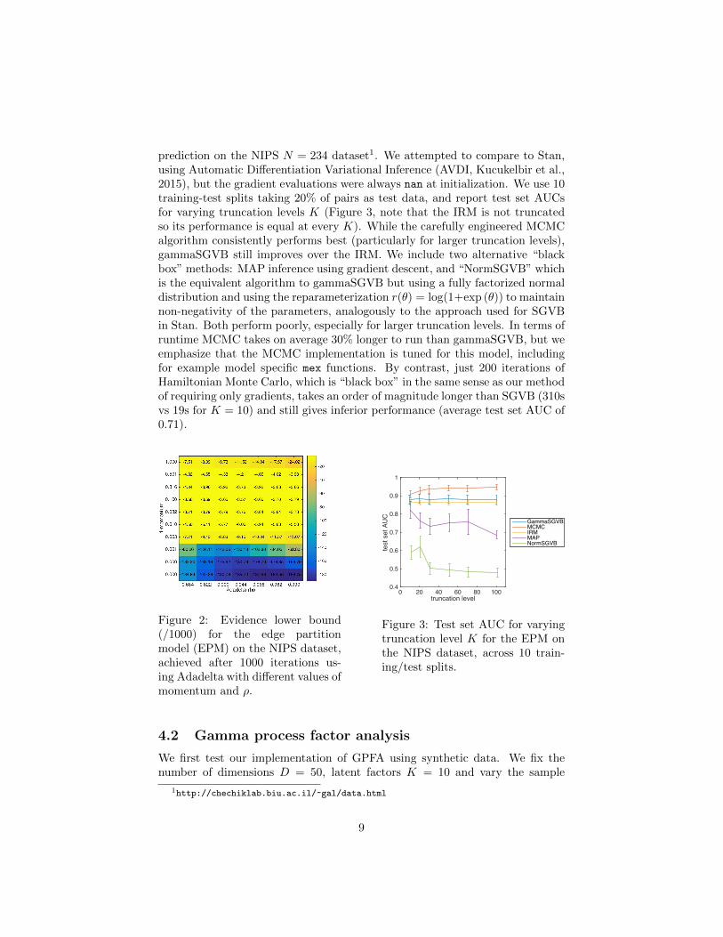
prediction on the NIPS N = 234 dataset1. We attempted to compare to Stan,using Automatic Differentiation Variational Inference (AVDI, Kucukelbir et al.,2015), but the gradient evaluations were always nan at initialization. We use 10training-test splits taking 20% of pairs as test data, and report test set AUCsfor varying truncation levels K (Figure 3, note that the IRM is not truncatedso its performance is equal at every K). While the carefully engineered MCMCalgorithm consistently performs best (particularly for larger truncation levels),gammaSGVB still improves over the IRM. We include two alternative “blackbox” methods: MAP inference using gradient descent, and “NormSGVB” whichis the equivalent algorithm to gammaSGVB but using a fully factorized normaldistribution and using the reparameterization r(θ) = log(1+exp (θ)) to maintainnon-negativity of the parameters, analogously to the approach used for SGVBin Stan. Both perform poorly, especially for larger truncation levels. In terms ofruntime MCMC takes on average 30% longer to run than gammaSGVB, but weemphasize that the MCMC implementation is tuned for this model, includingfor example model specific mex functions. By contrast, just 200 iterations ofHamiltonian Monte Carlo, which is “black box” in the same sense as our methodof requiring only gradients, takes an order of magnitude longer than SGVB (310svs 19s for K = 10) and still gives inferior performance (average test set AUC of0.71).
Figure 2: Evidence lower bound(/1000) for the edge partitionmodel (EPM) on the NIPS dataset,achieved after 1000 iterations us-ing Adadelta with different values ofmomentum and ρ.
truncation level0 20 40 60 80 100
test se
t A
UC
0.4
0.5
0.6
0.7
0.8
0.9
1
GammaSGVBMCMCIRMMAPNormSGVB
Figure 3: Test set AUC for varyingtruncation level K for the EPM onthe NIPS dataset, across 10 train-ing/test splits.
4.2 Gamma process factor analysis
We first test our implementation of GPFA using synthetic data. We fix thenumber of dimensions D = 50, latent factors K = 10 and vary the sample
1http://chechiklab.biu.ac.il/~gal/data.html
9
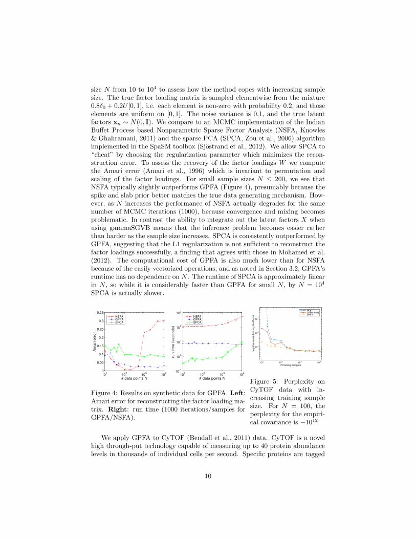
size N from 10 to 104 to assess how the method copes with increasing samplesize. The true factor loading matrix is sampled elementwise from the mixture0.8δ0 + 0.2U [0, 1], i.e. each element is non-zero with probability 0.2, and thoseelements are uniform on [0, 1]. The noise variance is 0.1, and the true latentfactors xn ∼ N(0, I). We compare to an MCMC implementation of the IndianBuffet Process based Nonparametric Sparse Factor Analysis (NSFA, Knowles& Ghahramani, 2011) and the sparse PCA (SPCA, Zou et al., 2006) algorithmimplemented in the SpaSM toolbox (Sjostrand et al., 2012). We allow SPCA to“cheat” by choosing the regularization parameter which minimizes the recon-struction error. To assess the recovery of the factor loadings W we computethe Amari error (Amari et al., 1996) which is invariant to permutation andscaling of the factor loadings. For small sample sizes N ≤ 200, we see thatNSFA typically slightly outperforms GPFA (Figure 4), presumably because thespike and slab prior better matches the true data generating mechanism. How-ever, as N increases the performance of NSFA actually degrades for the samenumber of MCMC iterations (1000), because convergence and mixing becomesproblematic. In contrast the ability to integrate out the latent factors X whenusing gammaSGVB means that the inference problem becomes easier ratherthan harder as the sample size increases. SPCA is consistently outperformed byGPFA, suggesting that the L1 regularization is not sufficient to reconstruct thefactor loadings successfully, a finding that agrees with those in Mohamed et al.(2012). The computational cost of GPFA is also much lower than for NSFAbecause of the easily vectorized operations, and as noted in Section 3.2, GPFA’sruntime has no dependence on N . The runtime of SPCA is approximately linearin N , so while it is considerably faster than GPFA for small N , by N = 104
SPCA is actually slower.
# data points N10
110
210
310
4
Am
ari
err
or
0
0.05
0.1
0.15
0.2
0.25
0.3
0.35NSFAGPFASPCA
# data points N10
110
210
310
4
run
tim
e (
se
co
nd
s)
10-1
100
101
102
103
NSFAGPFASPCA
Figure 4: Results on synthetic data for GPFA. Left:Amari error for reconstructing the factor loading ma-trix. Right: run time (1000 iterations/samples forGPFA/NSFA).
# training samples102 103 104 105
nega
tive
mea
n te
st lo
g lik
elih
ood
102
103
104
MLELedoit-WolfeGPFA
Figure 5: Perplexity onCyTOF data with in-creasing training samplesize. For N = 100, theperplexity for the empiri-cal covariance is −1012.
We apply GPFA to CyTOF (Bendall et al., 2011) data. CyTOF is a novelhigh through-put technology capable of measuring up to 40 protein abundancelevels in thousands of individual cells per second. Specific proteins are tagged
10

using heavy metals which are measured using time-of-flight mass spectrometry.The sample we analyze consists of human immune cells, so representing theheterogeneity between cells is relevant for understanding disease response. Ourdataset has N = 5.3 × 10⁵ cells and D = 40 protein expression levels. We runGPFA for 3000 iterations using Adadelta(ρ = 0.9, ε = 1× 10⁻⁴), K = 40 and aprior 1/σ2 ∼ G(.1, .1) on the noise variance. Runtime is around 10 seconds on aquad-core 2.5GHz i7 MacBook Pro. To assess performance we split the datasetinto a training and test set. Having fit the model on the training data, wecalculate the perplexity (average negative log likelihood over test data points)of the remaining (test) data under the learnt model by drawing S = 100 samplesW (s), σ2
(s) ∼ q, and obtaining the expected covariance matrix,
ˆCov(y) =1
S
S∑s=1
W (s)W (s) + σ2(s)I. (20)
We compare to two simple alternatives: using the maximum likelihood estimator(i.e. the empirical covariance), and Ledoit-Wolfe shrinkage (Ledoit & Wolf,2003). We see that for fewer than around N = 2000 training points GPFAoutperforms the empirical covariance or Ledoit-Wolfe. In real datasets it isoften the case that N is not significantly larger than D, or even N < D (usuallyreferred as the “large p, small n” regime), so GPFA’s strong performance forsmaller sample sizes is valuable. Finally in Figure 6 we show the empirical andestimated covariances, and the expected posterior factor loading matrix.
latent factors2 4 6 8 10
0
0.1
0.2
0.3
0.4
0.5
0.6
0.7
0.8
0.9
1
Figure 6: Estimated covariance structure on CyTOF data. GPFA modelsthe structure well, whilst regularizing the off diagonal components in partic-ular. Left: empirical covariance. Middle: covariance estimated under GPFA.Right: top 10 latent factor loadings. These are easier to interpret than theusual PCA loadings because of the enforced non-negativity.
11

5 Discussion
Variational inference has been considered a promising candidate for scalingBayesian inference to real world datasets for some time. However, only with theadvent of stochastic variational methods has this hope really started to becomea reality. Alongside minibatch based SVI allowing improved scalability, by usingMonte Carlo estimation SGVB can also allow a wider range of models to be eas-ily handled than standard VBEM. The only model specific derivation we requireis the gradient of the log joint, which is no more than is required for LBFGSor HMC. Indeed, automatic differentiation tools such as Theano (Bastien et al.,2012) could (and should!) be used to obtain these gradients. We have shownhere that these ideas apply to sparse continuous latent variables represented us-ing a gamma variational posterior, as well as to Gaussian variables. In additionwe have shown that the ability to easily handle non-conjugate likelihoods canhave advantages in terms of inference: in particular that collapsing models canimprove performance. While this is well known for Latent Dirichlet Allocation(Blei et al., 2003), leveraging this understanding has previously required carefulmodel specific derivations (see e.g. Teh et al. (2006)). An interesting potentialline of future research would be to combine the ideas presented here with thevariational autoencoder (Kingma & Welling, 2013) to allow scalable, nonlinear,sparse latent variable models, while additionally giving some ability to modelposterior dependencies.
References
Amari, Shun-ichi, Cichocki, Andrzej, Yang, Howard Hua, et al. A new learning al-gorithm for blind signal separation. Advances in Neural Information ProcessingSystems, pp. 757–763, 1996.
Bastien, Frederic, Lamblin, Pascal, Pascanu, Razvan, Bergstra, James, Goodfellow,Ian J., Bergeron, Arnaud, Bouchard, Nicolas, and Bengio, Yoshua. Theano: newfeatures and speed improvements. Deep Learning and Unsupervised Feature Learn-ing NIPS 2012 Workshop, 2012.
Bendall, Sean C, Simonds, Erin F, Qiu, Peng, El-ad, D Amir, Krutzik, Peter O, Finck,Rachel, Bruggner, Robert V, Melamed, Rachel, Trejo, Angelica, Ornatsky, Olga I,et al. Single-cell mass cytometry of differential immune and drug responses acrossa human hematopoietic continuum. Science, 2011.
Blei, David M, Ng, Andrew Y, and Jordan, Michael I. Latent dirichlet allocation.JMLR, 2003.
Blundell, C. and Teh, Y. W. Bayesian hierarchical community discovery. In Advancesin Neural Information Processing Systems, 2013.
Ding, Chris, Li, Tao, and Jordan, Michael I. Convex and semi-nonnegative matrixfactorizations. Pattern Analysis and Machine Intelligence, IEEE Transactions on,32(1):45–55, 2010.
12
Duchi, John, Hazan, Elad, and Singer, Yoram. Adaptive subgradient methods foronline learning and stochastic optimization. The Journal of Machine Learning Re-search, 12:2121–2159, 2011.
Goodman, Noah, Mansinghka, Vikash, Roy, Daniel, Bonawitz, Keith, and Tarlow,Daniel. Church: a language for generative models. arXiv preprint arXiv:1206.3255,2012.
Hoffman, Matthew, Bach, Francis R, and Blei, David M. Online learning for latentdirichlet allocation. In advances in neural information processing systems, pp. 856–864, 2010.
Hoffman, Matthew D, Blei, David M, Wang, Chong, and Paisley, John. Stochasticvariational inference. The Journal of Machine Learning Research, 14(1):1303–1347,2013.
Jordan, Michael I, Ghahramani, Zoubin, Jaakkola, Tommi S, and Saul, Lawrence K.An introduction to variational methods for graphical models. Machine learning, 37(2):183–233, 1999.
Kemp, Charles and Tenenbaum, Joshua B. Learning systems of concepts with aninfinite relational model. In 21st National Conference on Artificial Intelligence,2006.
Kingma, Diederik P and Welling, Max. Auto-encoding variational bayes.arXiv:1312.6114, 2013.
Knowles, David and Ghahramani, Zoubin. Nonparametric bayesian sparse factor mod-els with application to gene expression modeling. The Annals of Applied Statistics,5(2B):1534–1552, 2011.
Kucukelbir, Alp, Ranganath, Rajesh, Gelman, Andrew, and Blei, David M. Automaticvariational inference in stan. arXiv preprint arXiv:1506.03431, 2015.
Ledoit, Olivier and Wolf, Michael. Improved estimation of the covariance matrix ofstock returns with an application to portfolio selection. Journal of empirical finance,10(5):603–621, 2003.
Lunn, David J, Thomas, Andrew, Best, Nicky, and Spiegelhalter, David. Winbugs-abayesian modelling framework: concepts, structure, and extensibility. Statistics andcomputing, 10(4):325–337, 2000.
Minka, Tom, Winn, John, Guiver, John, and Knowles, David. Infer.NET 2.4, MicrosoftResearch Cambridge, 2010.
Mohamed, Shakir, Heller, Katherine, and Ghahramani, Zoubin. Bayesian and l1 ap-proaches to sparse unsupervised learning. ICML, 2012.
Morup, M, Schmidt, Mikkel N, and Hansen, Lars Kai. Infinite multiple membership re-lational modeling for complex networks. In Machine Learning for Signal Processing.IEEE, 2011.
Paisley, John, Blei, David, and Jordan, Michael. Variational Bayesian inference withstochastic search. In ICML 2012, 2012.
13

Ranganath, Rajesh, Gerrish, Sean, and Blei, David M. Black box variational inference.arXiv:1401.0118, 2013.
Robbins, Herbert and Monro, Sutton. A stochastic approximation method. The Annalsof Mathematical Statistics, 22(3):400–407, 1951.
Salimans, Tim and Knowles, David A. Fixed-form variational posterior approximationthrough stochastic linear regression. Bayesian Analysis, 8(4):837–882, 2013.
Sjostrand, Karl, Clemmensen, Line Harder, Larsen, Rasmus, and Ersbøll, Bjarne.Spasm: A matlab toolbox for sparse statistical modeling. Journal of StatisticalSoftware Accepted for publication, 2012.
Stan Development Team. Stan: A c++ library for probability and sampling, 2014.
Teh, Yee W, Newman, David, and Welling, Max. A collapsed variational bayesianinference algorithm for latent dirichlet allocation. In NIPS, 2006.
Tieleman, T and Hinton, G. Lecture 6.5 - rmsprop, 2012.
Zeiler, Matthew D. Adadelta: an adaptive learning rate method. arXiv preprintarXiv:1212.5701, 2012.
Zhou, Mingyuan. Infinite edge partition models for overlapping community detectionand link prediction. In AISTATS 2015. JMLR, 2015.
Zou, Hui, Hastie, Trevor, and Tibshirani, Robert. Sparse principal component analysis.JCGS, 2006.
14