STOCHASTIC BUDGETING AND INPUT BREAKEVEN ANALYSIS IN …
99
STOCHASTIC BUDGETING AND INPUT BREAKEVEN ANALYSIS IN NORTH DAKOTA POTATO PRODUCTION A Thesis Submitted to the Graduate Faculty of the North Dakota State University of Agriculture and Applied Science By Alan Bingham In Partial Fulfillment of the Requirements for the Degree of MASTER OF SCIENCE Major Department: Plant Sciences March 2017 Fargo, North Dakota
Transcript of STOCHASTIC BUDGETING AND INPUT BREAKEVEN ANALYSIS IN …
STOCHASTIC BUDGETING AND INPUT BREAKEVEN ANALYSIS IN NORTH DAKOTA
POTATO PRODUCTION
A Thesis
Submitted to the Graduate Faculty
of the
North Dakota State University
of Agriculture and Applied Science
By
Alan Bingham
In Partial Fulfillment of the Requirements
for the Degree of
MASTER OF SCIENCE
Major Department:
Plant Sciences
March 2017
Fargo, North Dakota

North Dakota State University
Graduate School
Title
STOCHASTIC BUDGETING AND INPUT BREAKEVEN ANALYSIS
IN NORTH DAKOTA POTATO PRODUCTION
By
Alan Bingham
The Supervisory Committee certifies that this disquisition complies with North Dakota
State University’s regulations and meets the accepted standards for the degree of
MASTER OF SCIENCE
SUPERVISORY COMMITTEE:
Andrew Robinson
Chair
Ryan Larsen
Asunta Thompson
Approved:
July 10, 2017 Richard Horsley
Date Department Chair

iii
ABSTRACT
Enterprise budgets were developed for non-irrigated red and irrigated russet potato
production, based on North Dakota model farms. Costs and revenues vary among producers, thus
budgets are intended to serve as a template for producers to use and manipulate to suit their
individual circumstances. These budgets and stochastic (Monte Carlo) simulation were utilized
in order to analyze and quantify financial risk in each respective enterprise. Simulated net returns
for non-irrigated production ranged from -$1,324 to $2,757 per acre, while irrigated returns were
between -$551 and $1,616 per acre. On farms where fumigation is a typical practice, it is one of
the largest expenses to the enterprise. A break-even analysis was conducted based on market
price and possible increases in yield and yield quality. The breakeven curve is downward
sloping, as market price increases. Ideal product selection, based on assumed benefits, may vary
depending on expected market price.

iv
ACKNOWLEDGEMENTS
I am grateful to the members of my supervisory committee, Dr. Andrew Robinson, Dr.
Ryan Larsen, and Dr. Asunta Thompson, for their flexibility in the oversight of this project and
the investment of their time in me. I express my thanks to the members of the Northern Plains
Potato Growers Association for the historical data they shared with me and the validation they
provided. Finally, I wish to offer acknowledgement and gratitude to TriEst Ag Group for
providing the funding for my research.

v
DEDICATION
To my beautiful bride Diane, for her continued support, encouragement, and confidence in me;
and to my three wonderful little girls who are some of my greatest cheerleaders without even
realizing it. And to my parents who instilled in me, from a young age, a desire to pursue higher
education.

vi
TABLE OF CONTENTS
ABSTRACT ................................................................................................................................... iii
ACKNOWLEDGEMENTS ........................................................................................................... iv
DEDICATION ................................................................................................................................ v
LIST OF TABLES ....................................................................................................................... viii
LIST OF FIGURES ....................................................................................................................... ix
LIST OF APPENDIX TABLES .................................................................................................... xi
INTRODUCTION .......................................................................................................................... 1
Objectives .................................................................................................................................... 3
Literature Cited ........................................................................................................................... 4
NON-IRRIGATED RED POTATO PRODUCTION AND RISK ................................................. 5
Abstract ....................................................................................................................................... 5
Introduction ................................................................................................................................. 5
Materials and Methods .............................................................................................................. 10
Model Farm ........................................................................................................................... 10
Deterministic Budget ............................................................................................................. 10
Stochastic Factors .................................................................................................................. 17
Results and Discussion .............................................................................................................. 22
Distribution of Simulated Net Returns .................................................................................. 23
A Wheat Comparison ............................................................................................................ 25
Magnitude of Input Effect on Net Returns ............................................................................ 26
Conclusion ................................................................................................................................. 28
Literature Cited ......................................................................................................................... 30
IRRIGATED RUSSET POTATO PRODUCTION AND RISK .................................................. 32
Abstract ..................................................................................................................................... 32

vii
Introduction ............................................................................................................................... 32
Materials and Methods .............................................................................................................. 36
Model Farm ........................................................................................................................... 36
Deterministic Budget ............................................................................................................. 37
Stochastic Factors .................................................................................................................. 45
Results and Discussion .............................................................................................................. 49
Distribution of Simulated Net Returns .................................................................................. 50
A Wheat Comparison ............................................................................................................ 53
Magnitude of Input Effect on Net Returns ............................................................................ 54
Conclusion ................................................................................................................................. 55
Literature Cited ......................................................................................................................... 56
FUMIGATION COST AND BREAK-EVEN ANALYSIS ......................................................... 59
Abstract ..................................................................................................................................... 59
Introduction ............................................................................................................................... 59
Management of PED ............................................................................................................. 61
Materials and Methods .............................................................................................................. 62
Fumigation Cost .................................................................................................................... 62
Break-even Discussion .......................................................................................................... 63
Conclusion ................................................................................................................................. 67
Literature Cited ......................................................................................................................... 68
APPENDIX ................................................................................................................................... 70

viii
LIST OF TABLES
Table Page
1. Price statistics measured in $/cwt for red potatoes sold in the fresh market from
2003 to 2016 based on once a month snapshot for each month of the marketing
year (September to May). ................................................................................................. 18
2. Yield statistics for non-irrigated potatoes grown in North Dakota from 1994 to 2009
(USDA, 2016). .................................................................................................................. 21

ix
LIST OF FIGURES
Figure Page
1. Historical size A prices for fresh red potatoes when grown in the Red River
Valley of North Dakota or Minnesota and the best fit (Weibull) distribution. ................. 20
2. Historical size B prices for fresh red potatoes when grown in the Red River
Valley of North Dakota or Minnesota and the best fit (Kumaraswamy)
distribution. ....................................................................................................................... 20
3. Historical yield of non-irrigated potatoes in North Dakota in cwt per acre, and the
best fit (Laplace) distribution (NASS, 2016). ................................................................... 22
4. Probability density of simulated net returns, in dollars per acre, of non-irrigated
red potatoes, in the Red River Valley of North Dakota, based on stochastic price
and yield. ........................................................................................................................... 24
5. Weibull and normal distributions fit to the output results for net returns of non-
irrigated red potatoes in the Red River Valley of North Dakota. ..................................... 25
6. Overlaid probability density of net returns for hard red spring wheat and non-
irrigated red potato. ........................................................................................................... 27
7. Tornado graph of the magnitude of the effect of each stochastic input (A, B, and
C price and yield) on net returns ($/ac) for non-irrigated red potato production in
the Red River Valley of North Dakota. ............................................................................ 28
8. Values sampled in the stochastic budget simulation for the price of processing
potatoes when grown in North Dakota, based on a triangular distribution. ..................... 47
9. Randomly sampled yield values used in the stochastic budget simulation for
irrigated russet potatoes in North Dakota, based on a triangular distribution. ................. 48
10. Probability density of simulated net returns, in dollars per acre, of irrigated russet
potatoes grown in North Dakota for the processing market. ............................................ 51
11. The best fit (beta general) and normal distributions, fit to the simulated net returns
($/ac) for irrigated russet potatoes grown in North Dakota. ............................................. 52
12. Overlaid probability density of net returns for hard red spring wheat and irrigated
russet potato. ..................................................................................................................... 54
13. Tornado graph of the magnitude of the effect of each stochastic input (price and
yield) on irrigated russet potato net returns ($/acre) in North Dakota. ............................. 55
x
14. Example curve of yield increase needed to break even on metam sodium
application. Based on a 350 cwt per acre total yield without fumigation, assumes
76% marketable yield rate without fumigation, and assumes a 7% increase in the
marketable yield rate due to fumigation. Fumigation cost of $360 per acre .................... 64
15. Potato price required to break even on fumigation depending on total yield
increase realized for 3 different marketable yield rates. Based on 350 cwt per acre
total yield without fumigation and assumes a 76% marketable yield rate without
fumigation. Fumigation cost of $360 per acre. ................................................................. 65
16. Yield increase needed to break even, subject to market price, for two different
fumigant products with differing increases in marketable yield rate. ............................... 66
17. Yield increase needed to break even on fumigation with non-irrigated red potatoes
and irrigated russet potatoes. Based on 350 cwt per acre yield for irrigated russets
without fumigation, 190 cwt per acre yield for irrigated reds without fumigation,
76% marketable yield for each variety without fumigation, and 7% increase in
marketable yield rate due to fumigation. Fumigation cost of $360 per acre. ................... 67

xi
LIST OF APPENDIX TABLES
Table Page
A1. NDSU model farm budget for non-irrigated red potato production. ................................ 70
A2. Fertility plan and cost of product for non-irrigated red potato production. ...................... 72
A3. Pesticide application rates and cost of product for non-irrigated red potato
production. ........................................................................................................................ 73
A4. Whole farm equipment overhead costs for non-irrigated red potato production. ............. 74
A5. Whole farm equipment operating costs for non-irrigated potatoes in dollars. .................. 75
A6. Equipment usage and labor for non-irrigated red potato production. ............................... 76
A7. NDSU model farm budget for irrigated russet potato production. ................................... 77
A8. Fertility plan and cost of product for irrigated russet potato production. ......................... 79
A9. Pesticide application rates and cost of product for irrigated russet potato
production. ........................................................................................................................ 80
A10. Whole farm equipment overhead costs for irrigated russet potatoes in dollars. .............. 81
A11. Whole farm equipment operating costs for irrigated russet potatoes in dollars. .............. 84
A12. Equipment usage and labor for irrigated russet potato production. ................................. 87
A13. Price required to break even on fumigation based on expected total yield
increases and marketable yield rate improvements. ......................................................... 88
1
INTRODUCTION
The United States potato industry produced over 44 billion pounds of potatoes in 2015,
on just over one million acres of farm land (2016 Potato Statistical Yearbook). In that same year,
Americans consumed 113.8 pounds of potatoes per capita. Approximately 30% of total
consumption were fresh potatoes, 42% were frozen potato products such as French fries and hash
browns, 18% were chips and shoestrings, and about 10% were dehydrated (2016 Potato
Statistical Yearbook). Annual per capita consumption has been declining in the United States
since the early 2000s, but increased in 2015 above 2014 and 2013 levels. Potatoes are a $3.8
billion industry in the United States (2016 Potato Statistical Yearbook).
North Dakota is the fourth largest potato producing state in the United States. In 2015,
2.7 billion pounds of potatoes were grown in the state, with a farm gate value of more than $258
million (2016 Potato Statistical Yearbook). Potatoes are an important part of agriculture and the
economy in North Dakota. As a generalization, there are two types of production systems in ND,
non-irrigated and irrigated. The majority of the potatoes grown for the fresh market in ND are
non-irrigated red-skinned potatoes. The Red River Valley of North Dakota and Minnesota is the
largest red potato growing region in the country (NPPGA, 2017). Some of the common red-
skinned cultivars grown are Red Norland, Dark Red Norland, Red LaSoda, and Viking. Most of
the potatoes grown outside of the Red River Valley are irrigated and grown for French fry
processing (NPPGA, 2017). Some of the common cultivars grown for processing are Russet
Burbank, Ranger Russet, Umatilla Russet, and Bannock Russet.
Potatoes are a high input crop, they are susceptible to a wide range of pests and diseases,
and require frequent pesticide applications. They require specialized field and handling
equipment. To maximize quality, potatoes should be stored in climate controlled storages. They

2
are perishable and have a high water content, making the raw product expensive to transport long
distances. Inputs and production practices vary considerably among potato producing regions of
the country due to climate, regional pest and disease presence, access to human, capital, and
natural resources; and the intended market use of the product. There are also significant
differences between irrigated and non-irrigated systems. The cost of production for a non-
irrigated red grower in North Dakota will look quite different from the irrigated russet grower in
the same region because the red grower has lower input costs and a shorter growing season from
planting to maturity. There will also be differences among operations due to efficiency and
economies of scale. In other words, a larger operation will often be able to utilize resources more
efficiently by being able to spread costs over a greater volume of output, or secure lower input
prices through bulk purchasing. Cost and revenue may also vary due to diversity in contracts,
marketing, and individual agreements with suppliers. Due to these and other factors, it is difficult
to estimate a budget that is widely applicable with relative accuracy. Budgets based on regional
inputs and a clear set of assumptions that individual potato growers can manipulate to suit their
needs and reflect their own constraints and circumstances are needed.
Deterministic enterprise budgets are often made to project an expectation of the financial
revenues and costs for the coming year; however, in reality it only represents one snapshot of
many possible outcomes for the farm. Some elements of a budget are fairly predictable and can
be planned for with some degree of certainty, while others may be quite variable, unpredictable,
and outside the realm of control of the potato grower. This fact makes potato production, and
most other agricultural enterprises, financially risky to engage in. Risk is a term often used to
describe elements of potato production, but it is not often spoken of in such a way as to
understand how much is actually at stake, or how one decision may be more or less risky than
3
another. Stochastic budgeting provides a method to quantify the level of risk by simulating many
possible outcomes, based on the statistical distributions of possible values for highly variable
budget items. Several researchers advocate the use of stochastic budgeting as a tool for the
analysis of risk. Lien (2003) demonstrated the usefulness of stochastic budgeting to evaluate
production decisions on a Norwegian dairy farm. Grove et al. (2007) employed stochastic
budgeting as a tool for the analysis of conversion from beef farming to game ranching in South
Africa.
One budget item of particular importance to potato production, due to the high cost
associated with it, is fumigation. Fumigation accounts for approximately 17% of total operating
costs in the ND model farm budget for irrigated russet potatoes. Many growers have adopted the
practice of fumigating their potato fields in order to protect their potato plants from a number of
yield limiting diseases and pests; however, some growers may be hesitant to adopt the practice
because of the high cost. Soil fumigation is thought to improve both total yield and quality, but
the question is whether the benefits gained are enough to offset the cost incurred.
Objectives
North Dakota State University does not currently have published enterprise budgets for
potatoes produced under non-irrigated or irrigated conditions. The first objective of this study
was to create enterprise budgets for both non-irrigated red potato production and irrigated russet
potato production based on a representative model farm. The second objective of this study was
to employ the enterprise budgets and stochastic simulation to quantify and analyze the risk of
non-irrigated red potato production and irrigated russet potato production. The third objective of
this study was to provide a framework that could be used by producers as a guideline to conduct
4
a breakeven analysis of fumigation in their own operation, based on expected changes in yield,
quality, and potato prices.
The remainder of this thesis is organized as follows. Chapter 1 (Non-Irrigated Red Potato
Production and Risk) discusses the development of the enterprise budget and risk evaluation
through stochastic simulation for non-irrigated red potato production. Chapter 2 (Irrigated Russet
Potato Production and Risk) discusses the irrigated russet potato budget and the stochastic
evaluation of risk in that enterprise. Chapter 3 (Fumigation Cost and Break-Even Analysis) is a
breakeven analysis of fumigation based on potato price and yield increases and improvements.
Literature Cited
Grove, B., P. R. Taljaard, and P. C. Cloete. 2007. A Stochastic Budgeting Analysis of Three
Alternative Scenarios to Convert from Beef-Cattle Farming to Game Ranching. Agrekon,
46(4):514-531.
Lein, G. 2003. Assisting whole-farm decision making through stochastic budgeting. Agricultural
Systems 76:399-413.
National Potato Council. 2016. 2016 Potato Statistical Yearbook. July 2016. Washington D.C.
NPPGA (Northern Plains Potato Growers Association). 2017. Quick Facts. Retrieved from
http://nppga.org/aboutus/quickfacts.php.
5
NON-IRRIGATED RED POTATO PRODUCTION AND RISK
Abstract
It is commonly accepted that potato production is a high risk enterprise. Quantifying this
risk can increase understanding so that producers may rank the relative risk of potato production
against the risk of other opportunities. Currently, there is not a published enterprise budget for
non-irrigated red potato production in North Dakota. An enterprise budget was first developed
based on a representative model farm in the Red River Valley. Distributions were derived for the
budget to represent ranges for possible price by tuber size and total yield. These distributions
were sampled randomly in a Monte Carlo simulation with 5,000 iterations, to derive a range of
possible net returns, in order to quantify the risk the enterprise is exposed to. The mean net return
was $205 per acre with a standard deviation of $638 per acre. Simulated net returns were widely
spread from a loss of $1324, to a gain of $2757 per acre. Non-irrigated potato production is a
risky enterprise.
Introduction
The Red River Valley of North Dakota and Minnesota is the largest red potato growing
region in the United States, with these two states producing nearly 40% of all red potatoes grown
in the US (National Potato Council, 2016). Approximately 64% of the potato acreage grown in
North Dakota is grown under non-irrigated conditions (USDA, 2016). Non-irrigated potato farms
in the state primarily produce red potatoes for the fresh market (NPPGA, 2017). Potatoes are a
high input crop requiring frequent chemical treatments, specialized equipment, expensive climate
controlled storages, and careful handling to preserve quality. An enterprise budget is an
important financial tool for producers to use in planning for these challenges.
6
Enterprise budgets provide a summary of all revenues and costs related to the enterprise
for a given financial period, usually one year for agricultural enterprises. They are not a
reflection of the entire farm. The cost of resources that are shared across multiple enterprises on
the farm, such as tractors or tillage implements, are allocated proportionally, according to their
use in each enterprise. In addition to a whole farm budget, an enterprise budget is important
because it allows a producer to analyze the performance of each operation independently of
others on the farm. Crop enterprise budgets have been published for irrigated potatoes in other
states (Patterson, 2013; Galinato and Tozer, 2016; Bogash et al. 2013), but little work has been
done on developing an enterprise budget for non-irrigated red potato production in North Dakota
or elsewhere.
Although a traditional enterprise budget is a valuable tool, its utility for risk management
is somewhat limited, in that it only represents a single, fixed scenario; however, it provides a
starting point for additional analysis. There are a number of unpredictable and uncontrollable
factors causing variability and risk within the budget. It is often said that potato production is a
“high risk, high reward” business, but what does that actually mean? It is true that there is a high
level of risk involved in commercial potato production due to high input costs, variable yields,
and volatile markets. The recent reduction in overall commodity prices has heightened the
awareness of maintaining sustainable profit margins and managing risk. However, in order to
accomplish this, it is important first to define what risk is in the context of an agricultural
enterprise.
There is much discussion on the subject of risk in economics and there is not a single
accepted definition of the term. The terms risk and uncertainty are often used interchangeably to
describe a situation where the outcome is unknown; however, Knight (1921), and subsequent

7
researchers, suggested a distinction between these two terms based upon information available
from similar past situations. Knight proposed that if a decision maker faced a choice with
multiple possible outcomes, which was similar to something that had occurred in the past, from
which a probability density could be generated, the decision maker faced a risky decision.
Additionally, uncertainty was represented when a decision maker faced a unique situation with
no precedent and multiple possible outcomes (Knight 1921). Knightian risk is measurable, while
uncertainty is immeasurable, and thus impossible to calculate. Risky decisions, events, or
outcomes can be graded as more risky or less risky than another, while uncertain events cannot.
Robinson and Barry (1987) pointed out that decision makers must often make probability
judgments with little or no empirical support or precedent. These would be situations that Knight
would consider uncertain; however, once the judgment has been made by the decision maker, the
decision making process is nearly the same, whether facing risk or uncertainty (Robinson and
Barry 1987). For this reason, many economists do not maintain the distinction between risk and
uncertainty, and often use the terms interchangeably. Robinson and Barry (1987) go on to
propose the importance of distinguishing between the two terms. “[They] define as risky, those
uncertain events whose outcomes alter the decision maker’s well-being” (Robinson and Barry
1987). This is different than the definition proposed by Knight (1921) and others where the two
terms are mutually exclusive. Instead, based on Robinson and Barry’s (1987) definition, risky
events are a subset of uncertain events, with uncertain events being those whose outcome is not
known with certainty.
Agricultural producers are subject to a high degree of risk due to many factors, such as
the biological nature of the production process, short run inelastic supply and demand, and
variances of weather (Myers et al. 2010). In order to be successful in agricultural markets, it is

8
important for producers to understand risk, and in what ways and to what degree their enterprise
or business is exposed. Even with identical information, sometimes individual producers make
decisions different from one another, under similar circumstances. This is due to differences in
risk preferences among producers and the probability they assign to future events (Kazmierczak
and Soto 2001). It is important for a producer to understand his or her individual risk
preferences. Risk preferences are based on the level of risk aversion felt by an individual, and
varies from person to person. Some of the factors that influence risk aversion are age, wealth,
income, and education (Riley and Chow, 1992). There must be some means of quantifying risk
in a manner that producers may rank potential “risky” decisions from least risky to most risky, so
that they might make an informed decision based on their individual risk preferences.
One method for analyzing risky decisions is through the use of Monte Carlo simulation,
also known as stochastic simulation. “Monte Carlo simulation encompasses any technique of
statistical sampling employed to approximate solutions to quantify problems” (Kwak and Ingall
2007). Stochastic (or Monte Carlo) budgeting is a means by which that variability can be
accounted for. Net returns can be calculated as a range of possibilities, and their probability of
occurrence, rather than simply as a deterministic value. In this type of simulation, a model
representing a real-life situation is developed with certain “risky” variables as inputs. Those
variables are each defined by specified distributions of possible values. Distributions can have a
number of shapes such as normal, beta, triangle, uniform, and others. Values are drawn at
random from the distribution and inputted into the model, simulating the entire system a large
number of times, or iterations. Each iteration represents a possible outcome for the model. The
range of outputs, across all iterations can then be compiled into a distribution, to indicate not
only what may happen, but also how likely it is to happen, based on the probabilities assigned to
9
the inputs. This provides a metric with which to rank potentially “risky” decisions, from least
risky to most risky, relative to one another. Kazmieczak and Soto (2001) utilized stochastic
budgeting to compare riskiness of returns to various sizes of channel catfish production
operations in the Mississippi Delta. Monte Carlo simulation can be a very powerful tool in trying
to understand the potential effects of uncertainty and risk, but it is only as good as the model it is
simulating and the information that is fed into it (Kwak and Ingall 2007). It is of the utmost
importance to use the best data and other information available when fitting distributions from
which to sample from.
Stochastic simulations begin with a fixed or deterministic model. Once the deterministic
model is developed, simulation can begin by identifying risky variables and replacing their fixed
values with stochastic distributions. Potato growers are exposed to risk from a myriad of sources.
Weather is capricious; potatoes are a susceptible host to a variety of insects and harmful
diseases; there are wide and unpredictable market fluctuations; consumer perceptions and
unfavorable public policy can drive market declines; input costs are high and may vary without
respect to potato price; and markets can shift due to changes in technology and consumer
preferences. Within the construct of an enterprise budget, many of the most impactful risks faced
by producers could be represented directly or indirectly in yield and price received.
The first objective of this study was to develop a deterministic enterprise budget for non-
irrigated red potatoes produced for the fresh market, based on local input costs and constraints
faced by a representative model farm of a size and scale typical to the Red River Valley. The
second objective was to utilize the deterministic enterprise budget to build a stochastic budget
with which to simulate and quantify the level of risk involved in non-irrigated red potato
production.
10
Materials and Methods
Model Farm
In order to estimate the cost of production for non-irrigated red potatoes, a model farm
was created. This was not intended to represent any one grower, but to be a representative 2,000
acre farm in the Red River Valley of North Dakota. The soil type was a clay loam with a normal
seasonal (May through August) rainfall of 12.1 inches (NDAWN, 2017). The crop rotation is
potato, followed by sugarbeet, dry bean, and wheat for one year each. The farm was designed to
grow 500 acres of each crop each year.
Model farm production practices are typical of non-irrigated potato farms in the Red
River Valley of North Dakota. In the fall prior to the potato crop, wheat stubble was tilled in
using a disc, and chisel plowed. Fertilizer was applied according to soil test results. Potatoes
were planted during the last two weeks of May, based on appropriate temperature and moisture
conditions. Potatoes were planted using two 6-row planters, in 36 inch rows, with a seeding rate
of 24 hundredweight (cwt) per acre. Seed was treated with a fungicide prior to planting.
Insecticide and starter fertilizer were applied in-furrow at planting. Potatoes were hilled once in
June prior to herbicide application. Harvest took place in late August and early September using
two 4-row harvesters. Potatoes were hauled from the field using eight tandem axel trucks and
hauled to a co-op owned storage and wash plant. They were washed and sorted by grade, to be
sold in the fresh market.
Deterministic Budget
The model farm enterprise budget is intended to serve as a template for producers and is
meant to be manipulated to suit individual conditions. The budget is organized in the following
three sections: gross returns, operating inputs, and ownership costs (Table A1). The organization
11
and format is similar to Patterson’s (2013) costs and returns estimate. All values or costs are
calculated on a per acre basis. Additionally, main sections provide the value of, or cost per,
marketable cwt.
Gross Returns
Gross returns for the potato enterprise are the sum of revenue received from the sale of all
marketable grades of potato. Tubers produced by the model farm were sized into one of three
categories and sold in the fresh market based on these categories. The size designations are: size
C tubers, being those smaller than 1.875 inches in diameter; size B ranging from 1.875 to 2.25
inches in diameter; and size A from 2.25 to 3.5 inches in diameter. The market also distinguishes
Chef size as being those tubers larger than 3.5 inches; however, for simplicity in this simulation,
all tubers over 2.25 inches in diameter were considered size A. Total yield and market price for
each size class were considered variably and are discussed in detail in a later section.
Operating Inputs
Operating inputs are sometimes referred to as variable costs. These are costs and
expenses that vary directly with the level of production engaged in for the year. Typically, these
are actual cash expenses that must be paid throughout the year. These costs include seed,
fertilizer, pesticides, hired custom operation, machinery maintenance and fuel, labor, rented
storage, and wash plant costs.
Seed
Seed planted was field generation three Red Norland. Two-ounce seed pieces were
planted every nine inches in 36 inch rows. Price for seed, seed freight, and seed cutting were
arrived at through general consensus of surveyed growers.
12
Fertilizer
Fertilizer rates will vary from year to year, dependent upon the soil test and the
producer’s yield goals. Table A2 shows an average fertility application plan and cost of products.
Like many of the input costs, the price paid for each of these products varies from grower to
grower, depending on agreements with suppliers.
Pesticides
Pesticide expenses are summarized in the budget in the following four categories:
herbicide, insecticide, fungicide, and desiccant. Table A3 shows all pesticide costs for the model
farm calculated in a separate sheet from the budget, where they are broken down into individual
products, their recommended rate, and the estimated cost of the product. These are not intended
to serve as recommendations. The value on this budget line represents only the cost of the
product. The cost of application is covered in another section.
Custom Application
Broadcast fertilization and pesticide application was custom applied. One fertilizer
treatment took place in the early spring, at an estimated rate of $6.50 per acre (Table A2). All
pesticide treatments were applied with a ground spray applicator at the same price rate as the
fertilizer spreading ($6.50/acre) (Table A2). Soil testing was also included as a service in this
section, and takes place for each potato field annually, at an estimated cost of $10 per acre (Table
A2).
Machinery
Equipment costs summarized in the budget were calculated in separate spreadsheets
represented in part in Tables A4, A5, and A6. Within these spreadsheets, costs were separated
into two categories: cash overhead (fixed) (Table A4) and operating (or variable) (Table A5)

13
expense. Cash overhead consisted of capital recovery costs, and a second category that combined
taxes, insurance, and housing related to equipment. Capital recovery is the joint cost of
depreciation and interest, and was calculated using a capital recovery factor, which is a function
of interest rate and the economic life of the machine (Edwards, 2015). The annual capital
recovery cost is found by multiplying the total depreciation (new price – salvage value) by the
capital recovery factor, then adding that to the product of salvage value and interest rate
(Edwards, 2015).
Capital recovery = (depreciation x capital recovery factor) + (salvage value x interest rate)
Edwards (2015) indicates that there is a tremendous variation in housing and insurance costs;
however, to simplify, he combined them together as one percent of the average value of the
machine.
Housing and insurance = 0.01 x (purchase price + salvage value) / 2
Operating costs are those costs that vary with the degree of usage of the machine, they
are also sometimes referred to as variable costs. Operating costs were subdivided as repairs, fuel,
and lubrication costs. Repair costs vary greatly due to many factors, such as management
policies, soil type and terrain, rocks, and operator skill. The best data for estimating repair costs
are records of producer’s past repair expenses (Edwards, 2015). Due to the lack of historical
repair costs for the model farm, repair expenses were estimated based on purchase price of the
machine and estimated total hours of use. Accumulated repair cost is an upward sloping curve,
indicating that repair costs are relatively lower early in the life of the machine and much higher
on a relative basis as the end of the economic life of the machine is approached (Edwards, 2015).
It is important to keep in mind that the annual repair cost calculated is an estimation of an
14
average annual cost over the life of the machine. Edwards (2015) provides a table of
accumulated repair costs as a percentage of list price, based on the type of machine and the
accumulated hours of use. The annual repair cost is found by dividing the product of the list price
and the percentage from the table, by the years of life (Edwards, 2015).
Annual repairs = (new list price x table value) / economic life
Fuel costs were calculated in two different ways depending on the type of machine. Fuel
costs were assigned to each individual implement rather than to specific tractors, thus there was
no fuel cost assigned to the tractors alone. For implements pulled by tractors, fuel was calculated
in gallons per hour, by multiplying 0.044 by the maximum PTO horsepower of the diesel engine
(Edwards, 2015). The product was multiplied by hours of use to obtain total annual consumption.
For pickups and trucks, fuel consumption was calculated based on estimated miles driven and
estimated average miles per gallon. Average fuel economy was estimated for the pickups as 12
miles per gallon, and 5 miles per gallon for the trucks. This value attempts to capture road miles,
field miles, and idle time.
Fuel costtractors = 0.044 x maximum PTO horsepower x annual hours of use x diesel price per
gallon
Fuel costtrucks = miles driven / average miles per gallon x fuel price per gallon
Surveys indicate that lubrication costs for most farms are, on average, about 15% of fuel
costs (Edwards. 2015). This factor was used as the basis for calculating lubrication cost for this
farm.
Lubrication = 0.15 x total fuel cost
15
Equipment cash overhead and operating expenses (discussed above) were mostly
calculated on a whole farm basis. A portion of each of these expenses was allocated specifically
to the potato enterprise, based on the proportion of use in potato relative to the rest of the farm.
For pickups and fuel and service trucks, it was estimated that approximately 40% of use was for
potato operations, 40% of use was for the sugar beet enterprise, and 10% each was assigned to
dry bean and wheat production.
Potato usage of pickups and fuel and service trucks = total usage / 2.5
Tractor total usage was calculated based on usage in the potato enterprise. Hours required
for each operation in potato were calculated based on size of implement, speed of travel, and
efficiency. Usage for the rest of the farm was estimated from this. Potato usage for tractor 1 was
multiplied by 2.25, tractor 2 usage was multiplied by 2.50 because it is the primary tractor used
in the other crops, and tractor 3 usage was multiplied by 2.00 because it is primarily only used in
potato and sugar beet. Truck usage was calculated based on loads per day that could be hauled
depending on the distance to the storage and the efficiency of both the harvest and unloading
operations. It was estimated that usage in sugar beet would be roughly equivalent to the usage in
potato, so potato usage was multiplied by 2.00 to obtain total farm usage (the tandem axel trucks
on the model farm are only used in potato and sugarbeet production).
Total truck hours = potato loads per day x hours per load x potato harvest days x 2
Labor
Labor requirements were broken down into three categories: equipment operator, truck
driver, and general laborer. Equipment operator hours were simply derived by multiplying the
hours of use for each piece of equipment by a 1.15. This factor accounts for the additional labor

16
hours that are required for things such as greasing and fueling equipment. Truck driver hours
were calculated in a similar manner based on hours of truck use. Finally, general laborer hour
requirements were assumed to be equal to 25% of the sum of all other labor. Hourly rates for
each of the three divisions are based on estimated normal wages for the region (A. P. Robinson,
personal communication, 2016).
Storage and Washing
Grower co-ops were consulted to obtain storage and wash plant expenses. The model
farm does not own a storage or wash facility. These expenses are paid to the co-op. A flat rate of
90 cents per cwt is assigned for storage, and is charged based on the total yield out of the field.
Wash plant charges are charged based on the marketable yield, with culls and shrink subtracted,
as per the industry standard practice.
Other
Crop insurance is purchased by the acre for $120 (A. P. Robinson, personal
communication, 2016). Potato fees and assessments are charged by state and national checkoffs.
The total of the state and national checkoffs is around 8.5 cents per cwt of marketable potatoes
sold from the wash plant (A. P. Robinson, personal communication, 2016). Operating interest is
charged in the budget at a rate of 5% on all operating costs.
Ownership Costs
Ownership costs for an enterprise are those expenses that are incurred whether or not the
crop is produced. These typically do not vary with output. Ownership costs related to machinery
and equipment have been discussed previously. Land rent was estimated as the average rate that
might be paid for a potato crop in the area. Even for a producer who may own all of his or her
farm ground, it is important to consider land rent as an expense in the budget, because it is the

17
opportunity cost that is incurred by growing the crop, rather than renting it out to another grower,
or selling it.
The final ownership cost in the enterprise budget is the management fee. The
management fee is the wage paid to the grower or the manager for the management of the
operation. This is an important expense to include, even if the owner is the one who is providing
the management, because it helps provide a clearer picture of the profitability of the enterprise,
and accounts for the opportunity cost of the grower’s time. The management fee for the model
farm is equivalent to 5% of the operating costs (Patterson, 2013). It should be acknowledged
that in practice, basing wages of management on actual expenses may not be the wisest strategy
because it takes away some of the incentive for efficiency. This method was simply used to
estimate a value that might be commensurate with the scale of the operation. There is much less
variability in input costs than in revenue, and therefore they provide a more stable basis for
estimation of the management fee.
Stochastic Factors
In reality, producers do not live in a deterministic, or fixed, world. Potato producers face
uncertainty and risk from many sources. Some sources of risk are more volatile than others.
Stochastic simulation was used to account for variability and risk. Stochastic values in the budget
are represented by statistical distributions that capture the range of probable values rather than
one fixed value. The stochastic factors in this analysis are yield and price by size grade of potato.
The strength and dependability of a simulation lies largely in the reliability of the data from
which distributions are defined. Efforts were made to obtain accurate historical data,
representative of the region in consideration.

18
Price Data
Prices used in this budget may or may not reflect actual prices received by commercial
potato growers, due to differences in contracts or terminal markets. Within the fresh red potato
market there is a wide range of prices received depending on the size classification of the potato,
and the time of year they are marketed. Recently, the smaller B and C potatoes typically sell for a
premium in the market, above the price of A size tubers.
Historical price data were obtained from the Northern Plains Potato Growers Association
(NPPGA) for size A and size B red fresh potatoes. It provides a once a month snapshot of the
fresh market prices for each month in the marketing year for the years of 2003 to 2016. The
marketing year ran from September to May. The mean price of size A tubers for these years
across all months was $16.31 per cwt, ranging from a minimum of $8.50, to a maximum of
$29.00 per cwt. The mean price of size B tubers during this same time frame was $23.99 per cwt,
with prices ranging from $11.50 to $39.75 per cwt (Table 1) (A. P. Robinson, personal
communication 2016).
Table 1. Price statistics measured in
$/cwt for red potatoes sold in the fresh
market from 2003 to 2016 based on once
a month snapshot for each month of the
marketing year (September to May).
Size A Size B
Minimum 8.50 11.50
Maximum 29.00 39.75
Mean 16.31 23.99
St. Dev. 4.12 7.04
19
Historical data were analyzed using the BestFit function in the @Risk software package
(Palisade Corporation, 2016). The BestFit function compiles data in a histogram and estimates a
probability density function, then optimizes the goodness-of-fit of the data among a set of
theoretical statistical distribution functions. Several goodness-of-fit statistics were utilized in
order to determine the distribution function that most accurately represents the historical data.
Based on this analysis, the best fitting statistical distribution to represent the price of size A
potatoes was the Weibull distribution. The Weibull distribution is defined by a shape parameter
(alpha), and a scale parameter (beta) (Palisade Corporation, 2016). The Weibull distribution fit to
the historical data for the price of size A red potatoes is shown in Figure 1. The Kumaraswamy
distribution was the best fit for the size B historical prices (Figure 2). The Kumaraswamy
distribution is defined by two shape parameters (alpha 1 and alpha 2), and a minimum and
maximum value (Palisade Corporation, 2016). It is very flexible, similar to the beta distribution.
Historical price data were not available for C size potatoes. The price of these is represented in
the budget by a specified premium added to the sampled B price. The premium is defined by an
estimated triangular distribution with a minimum value of $15, a most likely value of $20, and a
maximum value of $25 per cwt A positive correlation was discovered in the data between the
price of A and B size potatoes, using the Batch Fit function in @Risk. Batch Fit allows for
several ranges of data to be analyzed together for fit, and derives a correlation matrix if
correlation is discovered between the variables. This correlation is accounted for in the stochastic
model using the RiskCorrmat function. RiskCorrmat links distribution functions to a correlation
matrix so that variable sampling is not treated independently.

20
Yield Data
Reliable yield data for potato is difficult to obtain because there is substantial variability
in yields between different fields, producers, and regions of the state. The best yield data to use
would be historical yields for the particular farm being simulated. However, since this
information is not available for the model farm, yield data was obtained from the United States
Figure 1. Historical size A prices for fresh red potatoes when grown in the Red River Valley of
North Dakota or Minnesota and the best fit (Weibull) distribution.
Distribution Statistics
Historical Data Weibull
Minimum 8.50 5.72
Maximum 29.00 +Infinity
Mean 16.31 16.31
Mode 14.00 [est] 15.89
Median 16.38 16.16
Std. Deviation 4.12 4.07
Skewness 0.10 0.23
Price ($/cwt)
Distribution Statistics
Historical Data Kumaraswamy
Minimum 11.50 11.36
Maximum 39.75 40.49
Mean 23.99 23.96
Mode 13.50 [est] 21.21
Median 24.25 23.55
Std. Deviation 7.04 6.96
Skewness 0.13 0.20
Figure 2. Historical size B prices for fresh red potatoes when grown in the Red River
Valley of North Dakota or Minnesota and the best fit (Kumaraswamy) distribution.
Price ($/cwt)
21
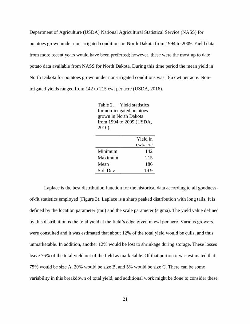
Department of Agriculture (USDA) National Agricultural Statistical Service (NASS) for
potatoes grown under non-irrigated conditions in North Dakota from 1994 to 2009. Yield data
from more recent years would have been preferred; however, these were the most up to date
potato data available from NASS for North Dakota. During this time period the mean yield in
North Dakota for potatoes grown under non-irrigated conditions was 186 cwt per acre. Non-
irrigated yields ranged from 142 to 215 cwt per acre (USDA, 2016).
Table 2. Yield statistics
for non-irrigated potatoes
grown in North Dakota
from 1994 to 2009 (USDA,
2016).
Yield in
cwt/acre
Minimum 142
Maximum 215
Mean 186
Std. Dev. 19.9
Laplace is the best distribution function for the historical data according to all goodness-
of-fit statistics employed (Figure 3). Laplace is a sharp peaked distribution with long tails. It is
defined by the location parameter (mu) and the scale parameter (sigma). The yield value defined
by this distribution is the total yield at the field’s edge given in cwt per acre. Various growers
were consulted and it was estimated that about 12% of the total yield would be culls, and thus
unmarketable. In addition, another 12% would be lost to shrinkage during storage. These losses
leave 76% of the total yield out of the field as marketable. Of that portion it was estimated that
75% would be size A, 20% would be size B, and 5% would be size C. There can be some
variability in this breakdown of total yield, and additional work might be done to consider these

22
percentages stochastically in the future. However, in this analysis, only total yield is stochastic
and the breakdown by size is treated deterministically.
Simulation
The stochastic simulation model is specified as
𝑁𝑅𝑖 = �̃�𝑖�̃�𝑖 − 𝑉𝐶 − 𝐹𝐶,
Where 𝑁𝑅𝑖 is the net return of simulation i, �̃�𝑖 and �̃�𝑖 are the simulated stochastic prices and
yields, VC is the variable cost, and FC is the fixed cost. The stochastic factors were defined by
their distribution functions; output for the simulation was specified as net returns above total cost
per acre. @Risk was used to simulate the model with 5,000 iterations, yielding 5,000 unique net
returns, based on the random sampling of the stochastic inputs.
Results and Discussion
Most farming operations prepare a pro forma budget when they are planning for the
upcoming year. These budgets are nearly always deterministic in nature, and as such, only
capture a single snapshot of a possible outcome, when in fact, there is a very wide range of
Distribution Statistics
Historical Data Laplace
Minimum 142.00 -Infinity
Maximum 215.00 +Infinity
Mean 185.94 185.50
Mode 185.00[est] 185.50
Median 185.50 185.50
Std. Deviation 16.86 15.47
Skewness (0.69) -
Figure 3. Historical yield of non-irrigated potatoes in North Dakota in cwt per acre, and the
best fit (Laplace) distribution (NASS, 2016).
Yield ($/cwt)
23
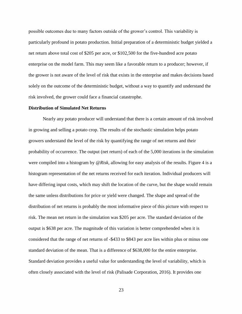
possible outcomes due to many factors outside of the grower’s control. This variability is
particularly profound in potato production. Initial preparation of a deterministic budget yielded a
net return above total cost of $205 per acre, or $102,500 for the five-hundred acre potato
enterprise on the model farm. This may seem like a favorable return to a producer; however, if
the grower is not aware of the level of risk that exists in the enterprise and makes decisions based
solely on the outcome of the deterministic budget, without a way to quantify and understand the
risk involved, the grower could face a financial catastrophe.
Distribution of Simulated Net Returns
Nearly any potato producer will understand that there is a certain amount of risk involved
in growing and selling a potato crop. The results of the stochastic simulation helps potato
growers understand the level of the risk by quantifying the range of net returns and their
probability of occurrence. The output (net return) of each of the 5,000 iterations in the simulation
were compiled into a histogram by @Risk, allowing for easy analysis of the results. Figure 4 is a
histogram representation of the net returns received for each iteration. Individual producers will
have differing input costs, which may shift the location of the curve, but the shape would remain
the same unless distributions for price or yield were changed. The shape and spread of the
distribution of net returns is probably the most informative piece of this picture with respect to
risk. The mean net return in the simulation was $205 per acre. The standard deviation of the
output is $638 per acre. The magnitude of this variation is better comprehended when it is
considered that the range of net returns of -$433 to $843 per acre lies within plus or minus one
standard deviation of the mean. That is a difference of $638,000 for the entire enterprise.
Standard deviation provides a useful value for understanding the level of variability, which is
often closely associated with the level of risk (Palisade Corporation, 2016). It provides one
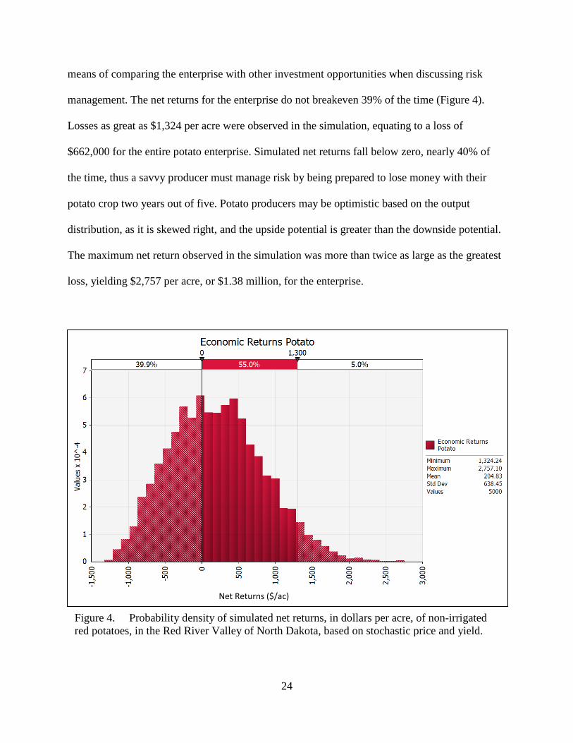
24
means of comparing the enterprise with other investment opportunities when discussing risk
management. The net returns for the enterprise do not breakeven 39% of the time (Figure 4).
Losses as great as $1,324 per acre were observed in the simulation, equating to a loss of
$662,000 for the entire potato enterprise. Simulated net returns fall below zero, nearly 40% of
the time, thus a savvy producer must manage risk by being prepared to lose money with their
potato crop two years out of five. Potato producers may be optimistic based on the output
distribution, as it is skewed right, and the upside potential is greater than the downside potential.
The maximum net return observed in the simulation was more than twice as large as the greatest
loss, yielding $2,757 per acre, or $1.38 million, for the enterprise.
Net Returns ($/ac)
Figure 4. Probability density of simulated net returns, in dollars per acre, of non-irrigated
red potatoes, in the Red River Valley of North Dakota, based on stochastic price and yield.

25
BestFit was used to fit a distribution to the output results for net returns. The Weibull
distribution provides the best fit. Typically, a farmer might expect his or her returns to be
somewhat normally distributed. From a risk management planning standpoint, the differences
between a normal and Weibull distribution would be fairly subtle (Figure 5). An assumption of
normally distributed returns might slightly overestimate potential losses, which may be
beneficial to the risk averse decision maker when planning for the future.
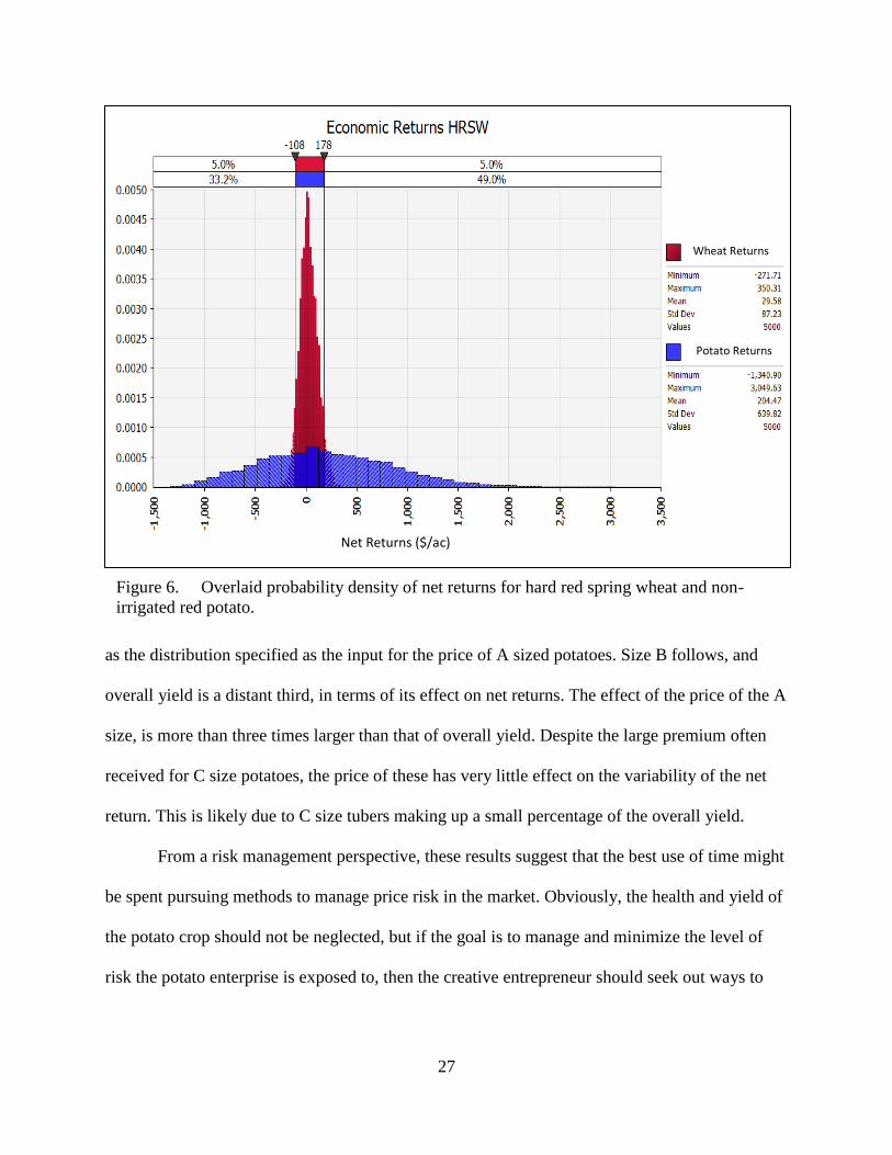
A Wheat Comparison
In order to put the range of simulated potato returns into perspective, a similar, simplified
analysis was conducted on hard red spring wheat. Wheat was chosen because it is another crop
grown by the model farm and is typical in the crop rotation, with potatoes, in North Dakota. An
Net Returns ($/ac)
Figure 5. Weibull and normal distributions fit to the output results for net returns of non-
irrigated red potatoes in the Red River Valley of North Dakota.
26
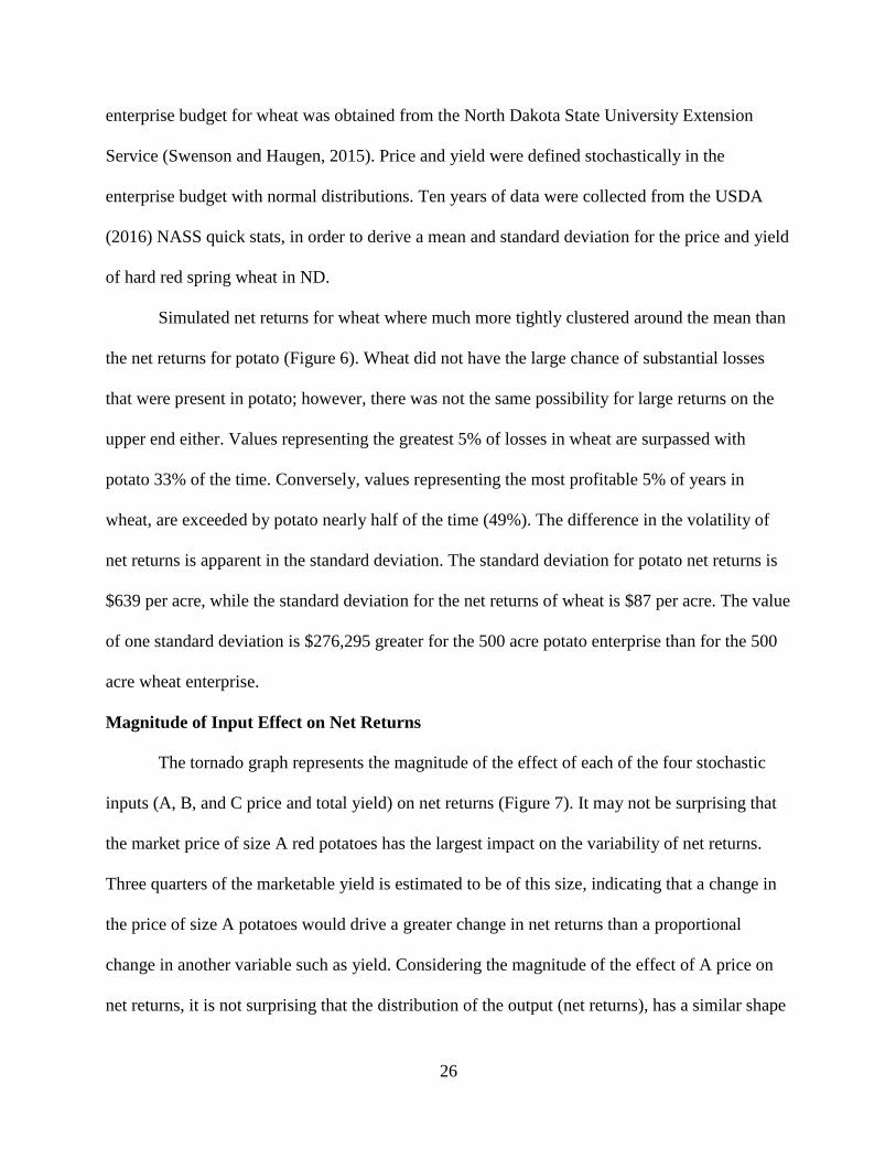
enterprise budget for wheat was obtained from the North Dakota State University Extension
Service (Swenson and Haugen, 2015). Price and yield were defined stochastically in the
enterprise budget with normal distributions. Ten years of data were collected from the USDA
(2016) NASS quick stats, in order to derive a mean and standard deviation for the price and yield
of hard red spring wheat in ND.
Simulated net returns for wheat where much more tightly clustered around the mean than
the net returns for potato (Figure 6). Wheat did not have the large chance of substantial losses
that were present in potato; however, there was not the same possibility for large returns on the
upper end either. Values representing the greatest 5% of losses in wheat are surpassed with
potato 33% of the time. Conversely, values representing the most profitable 5% of years in
wheat, are exceeded by potato nearly half of the time (49%). The difference in the volatility of
net returns is apparent in the standard deviation. The standard deviation for potato net returns is
$639 per acre, while the standard deviation for the net returns of wheat is $87 per acre. The value
of one standard deviation is $276,295 greater for the 500 acre potato enterprise than for the 500
acre wheat enterprise.
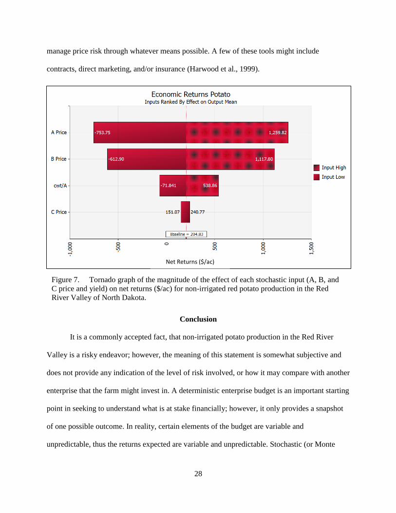
Magnitude of Input Effect on Net Returns
The tornado graph represents the magnitude of the effect of each of the four stochastic
inputs (A, B, and C price and total yield) on net returns (Figure 7). It may not be surprising that
the market price of size A red potatoes has the largest impact on the variability of net returns.
Three quarters of the marketable yield is estimated to be of this size, indicating that a change in
the price of size A potatoes would drive a greater change in net returns than a proportional
change in another variable such as yield. Considering the magnitude of the effect of A price on
net returns, it is not surprising that the distribution of the output (net returns), has a similar shape
27
as the distribution specified as the input for the price of A sized potatoes. Size B follows, and
overall yield is a distant third, in terms of its effect on net returns. The effect of the price of the A
size, is more than three times larger than that of overall yield. Despite the large premium often
received for C size potatoes, the price of these has very little effect on the variability of the net
return. This is likely due to C size tubers making up a small percentage of the overall yield.
From a risk management perspective, these results suggest that the best use of time might
be spent pursuing methods to manage price risk in the market. Obviously, the health and yield of
the potato crop should not be neglected, but if the goal is to manage and minimize the level of
risk the potato enterprise is exposed to, then the creative entrepreneur should seek out ways to
Wheat Returns
Potato Returns
Net Returns ($/ac)
Figure 6. Overlaid probability density of net returns for hard red spring wheat and non-
irrigated red potato.
28
manage price risk through whatever means possible. A few of these tools might include
contracts, direct marketing, and/or insurance (Harwood et al., 1999).
Conclusion
It is a commonly accepted fact, that non-irrigated potato production in the Red River
Valley is a risky endeavor; however, the meaning of this statement is somewhat subjective and
does not provide any indication of the level of risk involved, or how it may compare with another
enterprise that the farm might invest in. A deterministic enterprise budget is an important starting
point in seeking to understand what is at stake financially; however, it only provides a snapshot
of one possible outcome. In reality, certain elements of the budget are variable and
unpredictable, thus the returns expected are variable and unpredictable. Stochastic (or Monte
Net Returns ($/ac)
Figure 7. Tornado graph of the magnitude of the effect of each stochastic input (A, B, and
C price and yield) on net returns ($/ac) for non-irrigated red potato production in the Red
River Valley of North Dakota.

29
Carlo) budgeting uses simulation to account for the variability, or risk, within the budget. Risky
elements are considered as ranges of possible values rather than fixed amounts.
Price and yield are some of the most unpredictable or risky budget components, with the
greatest effect on net returns. Ranges of values for prices were obtained largely from monthly
historical prices for red potatoes in the Red River Valley. The fresh market is quite volatile and
the range of prices varied tremendously over the time frame considered. Total yield also varied
significantly, due, speculatively, to the unpredictability and unreliability of the weather and other
challenges with producing non-irrigated potatoes. The volatility in price and yield, makes
stochastic budgeting a valuable tool for potato producers to evaluate risk.
Simulation of the non-irrigated red potato enterprise on the model farm yielded a positive
mean net return, but also had a high standard deviation for net returns, making it difficult to
predict positive returns consistently from year to year. Variability in the prices of A and B sized
potatoes were the greatest factors in determining the variability of returns. A risk averse manager
would most efficiently allocate risk management efforts to managing exposure to price risk
through the utilization of contracts, direct marketing, insurance, and/or any other means
available. The health and yield of the crop should not be neglected, but it is responsible for much
less risk to net returns. The authors do not attempt to classify non-irrigated red potato production
as strictly low or high risk; however, these values provide a metric with which to measure the
enterprise against others where resources might be devoted, to form a relative ranking of risk.
Every decision maker has unique risk preferences based on their position and appetite for risk.
Individual preferences for each party invested in the success of the enterprise should be
understood and accounted for by the decision maker seeking to manage risk and maximize
returns.

30
Literature Cited
Bogash, S. M., W. J. Lamont Jr., R. M. Harsh, and L. F. Kime. 2013. Potato Production. Penn
State Extension. Code UA360.
Edwards, W. 2015. Estimating farm machinery costs. Ag Decision Maker, File A3-29. Iowa
State University Extension and Outreach.
Galinato, S. P., and P. R. Tozer. 2016. 2015 Costs estimates of producing fresh and processing
potatoes in Washington. Washington State University Extension (TB14).
Harwood, J., R. Heifner, K. Coble, J. Perry, and A. Somwaru. 1999. Managing risk in farming:
concepts, research, and analysis. Economic Research Service, U.S. Department of
Agriculture. Agricultural Economics Report No. 774.
Kazmierczak, R. F. and P. Soto. 2001. Stochastic economic variables and their effect on net
returns to channel catfish production. Aquac. Econ. Manag. 5:1-2, 15-36.
Knight F. H. 1921. Risk, Uncertainty, and Profit. Houghton Mifflin. Boston and New York.
Kwak, Y. H. and L. Ingall. 2007. Exploring Monte Carlo simulation applications for project
management. Risk Management 9(1):44-45.
Myers, R. J., R. J. Sexton, W. G. Tomek. 2010. A century of research on agricultural markets.
Am. J. Agric. Econ. 92(2):376-402.
National Potato Council. 2016. 2016 Potato Statistical Yearbook. July 2016. Washington D.C.
NDAWN (North Dakota Agricultural Weather Network). 2017. NWS Monthly Normal Weather
Data. Retrieved from https://ndawn.ndsu.nodak.edu/weather-data-nws-monthly-
normals.html.
NPPGA (Northern Plains Potato Growers Association). 2017. Quick Facts. Retrieved from
http://nppga.org/aboutus/quickfacts.php.
31
Palisade Corporation. 2016. @Risk 7.5.0. Palisade Corporation, Ithaca, NY.
Patterson, P. E. 2013. Eastern Idaho Southern Region: Bannock, Bingham, & Power Counties,
Russet Burbank Potatoes: Production and Storage Costs. University of Idaho 2013 Costs
and Returns Estimate EBB4-Po-13.
Riley, W. B. and K. V. Chow. 1992. Asset allocation and individual risk aversion. Financ. Anal.
J., 48(6):32-37.
Robinson, L.J. and P.J. Barry. 1986. The Competitive Firm’s Response to Risk. Macmillan
Publishers.
USDA (United States Department of Agriculture). 2016. National Agricultural Statistical Service
(NASS), Quick Stats. Retrieved from https://quickstats.nass.usda.gov/.
32
IRRIGATED RUSSET POTATO PRODUCTION AND RISK
Abstract
Potato production is a risky enterprise. This statement, while generally accepted as truth,
is rather vague and could mean many different things to different individuals. This study sought
to quantify this statement, such that a producer could rank potato enterprise risk against other
opportunities. North Dakota State University does not currently have a published enterprise
budget for irrigated russet potato production. An enterprise budget was created based on a
hypothetical model farm in southeastern North Dakota. Distributions were derived for the budget
to represent ranges of possible prices and yield. These distributions were sampled randomly in a
Monte Carlo simulation, with 5,000 iterations, to derive a range of possible net returns in order
to quantify the risk the enterprise is exposed to. The mean net return was $384 per acre, with a
standard deviation of $430 per acre.
Introduction
North Dakota ranks fourth in the U.S. in potato production volume. Potatoes generated
more than $258 million in production value in the state in 2015 (National Potato Council, 2016).
Potatoes are a high input crop requiring frequent chemical treatments, specialized equipment,
expensive climate controlled storages, and careful handling to preserve quality. An enterprise
budget is an important financial tool for a farm to assess the year and make plans for the future.
Enterprise budgets exist for irrigated potato production in other regions of the U.S., but North
Dakota does not have a current published budget specific to the region.
An enterprise budget is a financial statement reflective of all costs and revenues
associated with a particular enterprise for a given financial period, such as a year. Unlike a whole
farm budget, it is not representative of the profitability of the entire farm, but only of the specific
33
enterprise, considered in isolation. The costs of some resources, such as tractors or tillage
implements are shared among multiple enterprises across the farm. In these cases, costs are
allocated proportionately according to their level of use in each enterprise. An enterprise budget
enables a producer to analyze each operation independently of others on the farm in order to
ensure wise allocation of resources across the farm. Published potato enterprise budgets exist for
other states (Patterson, 2013; Galinato and Tozer, 2016; Bogash et al., 2013), but there is no
published enterprise budget for irrigated potato production in North Dakota.
Although a traditional enterprise budget is a valuable tool, its relevance in risk
management is somewhat limited, in that it only represents a single, fixed scenario; however, it
provides a starting point for additional analysis. There are many unpredictable factors, outside
the control of the producer, that lead to variability and risk within the budget. It has often been
said that potato production is a “high risk, high reward” business, but what does that actually
mean? Commercial potato production does present a high degree of risk, due to high input costs,
variable yields, volatile markets and susceptibility to many economically damaging pests. The
recent reduction in overall commodity prices has increased the awareness of managing risk and
maintaining sustainable profit margins. When seeking to manage risk, it is important first, to
define what risk is in the context of an agricultural enterprise.
Risk is a much discussed subject within the field of economics; however, there is not a
single accepted definition of the term. The word risk is often used synonymously with the word
uncertainty, to describe a situation where the outcome is unknown. Knight (1921), and
subsequent researchers, suggested a distinction between these two terms based upon information
available from similar past situations. Knight proposed that a risky decision is one in which the
decision maker faces a choice with multiple possible outcomes, and a similarity to past events, so
34
that a probability density may be generated for the occurrence of a given outcome. Additionally,
if facing a unique situation with multiple outcomes and no precedent, the decision maker faces
uncertainty (Knight 1921). Knightian risk is measurable, while uncertainty is immeasurable, and
thus impossible to calculate. Risky decisions, events, or outcomes can be graded as more risky or
less risky than another, while uncertain events cannot.
Robinson and Barry (1987) pointed out that decision makers must often make probability
judgments with little or no empirical support or precedent. These would be situations that Knight
would consider uncertain; however, once the judgment has been made by the decision maker, the
decision making process is nearly the same, whether facing risk or uncertainty (Robinson and
Barry 1987). For this reason, many economists do not maintain the distinction between risk and
uncertainty, and often use the terms interchangeably. Robinson and Barry (1987) go on to
propose the importance of distinguishing between the two terms. “[They] define as risky those
uncertain events whose outcomes alter the decision maker’s well-being” (Robinson and Barry
1987). This is different than the definition proposed by Knight (1921) and others where the two
terms are mutually exclusive. Instead, based on Robinson and Barry’s (1987) definition, risky
events are a subset of uncertain events, with an uncertain event being those whose outcome is not
known with certainty.
Agricultural producers are subject to a high degree of risk due to many factors such as the
biological nature of the production process, short run inelastic supply and demand, and variances
of weather (Myers et al. 2010). It is important for producers to understand the concept of risk,
and the degree to which their enterprise or business is exposed, in order to be successful in
agricultural markets. Even with all the same information, sometimes individual producers make
different decisions under similar circumstances. This is due to differences in risk preferences
35
among producers and the probability they assign to future events (Kazmierczak and Soto 2001).
It is important for a producer to understand his or her individual risk preferences. Risk
preferences are based on the level of risk aversion felt by an individual, and varies from person
to person. Some of the factors that influence risk aversion are age, wealth, income, and education
(Riley and Chow, 1992). Some method or means of quantifying risk is needed to enable
producers to rank potential “risky” decisions from least risky to most risky, in order to make
informed decisions, based on their individual risk preferences.
Monte Carlo simulation, also known as stochastic simulation, provides one means of
analyzing potential risky decisions. “Monte Carlo simulation encompasses any technique of
statistical sampling employed to approximate solutions to quantify problems” (Kwak and Ingall
2007). This type of simulation begins with the development of a model, representative of a real-
life scenario. One or more of the model inputs are “risky” variables, defined by a specified
statistical distribution, representative of the range of probable values for that input. There are a
number of distribution shapes that may be used, such as normal, beta, triangle, uniform, and
others. Once the model is developed and the distributions defined, computer software is used to
run the simulation, randomly sampling values from the distributions and running them as inputs
in the model. This process takes place a large number of times, or iterations. Each iteration
represents a possible outcome for the model. The range of outputs, across all iterations can then
be compiled into a distribution, to indicate not only what may happen, but also how likely it is to
happen, based on the probabilities assigned to the inputs. This provides a metric with which to
rank potentially “risky” decisions, from least risky to most risky, relative to one another.
Khabkazan et al. (2014) used stochastic budgeting to analyze financial benefits and risk levels of
alternative calving schedules in Canadian beef production. Monte Carlo simulation can be a very
36
powerful tool in trying to understand the potential effects of uncertainty and risk, but it is only as
good as the model it is simulating and the information that is fed into it (Kwak and Ingall 2007).
It is important to seek out the best data and other information when fitting the distributions from
which to sample.
Stochastic simulations begin with a fixed or deterministic model. Once the deterministic
model is developed, simulation can begin by identifying risky variables and replacing their fixed
values with stochastic distributions. Potato growers are exposed to risk from a myriad of sources.
Weather is capricious; potatoes are a susceptible host to a variety of insects and harmful
diseases; there are wide and unpredictable market fluctuations; consumer perceptions and
unfavorable public policy can drive market declines; input costs are high and may vary without
respect to potato price; and markets can shift due to changes in technology and consumer
preferences. Within the construct of an enterprise budget, many of the most impactful risks faced
by producers could be represented directly or indirectly in yield and price received.
The first objective of this study was to develop a deterministic enterprise budget for
irrigated russet potato produced for the processing market based on a representative model farm
of a size and scale typical to a North Dakota farm outside the Red River Valley. The second
objective was to utilize the deterministic enterprise budget to build a stochastic budget with
which to simulate and quantify the level of risk involved in irrigated potato production.
Materials and Methods
Model Farm
A model farm was created in order to estimate the cost of production for irrigated russet
potatoes produced for the processing market. Producers operate under unique conditions with
varying operating costs and marketing channels. The model farm budget is intended to serve as a

37
template and is meant to be manipulated by the grower to suit their individual conditions. The
8,000 acre model farm is meant to be typical of the size and scale that would be found in ND
outside the Red River Valley, but it is not intended to represent an individual grower. The soil
type is a sandy silt loam with a normal seasonal (May through August) rainfall of 12.3 inches
(NDAWN, 2017). The farm utilizes center pivot irrigation. The crop rotation is potato, followed
by corn, soybean, and wheat, for one year each. The model farm was designed to plant 2,000
acres of each crop annually.
Production practices of the model farm are typical of irrigated farms in ND. In the fall
prior to the potato crop, wheat stubble is tilled in using a disc and chisel plowed. In the late fall,
soil is deep-shank fumigated with metam sodium. Fertilizer is applied in the spring prior to
planting, based on soil test results. Potatoes are planted from late April to early May, based on
appropriate temperature and moisture conditions, at a seeding rate of 19 hundredweight (cwt) per
acre, in 36 inch rows, using four 6-row planters. Seed is treated with a fungicide prior to
planting. Insecticide and starter fertilizer is applied in-furrow, at planting. Potatoes are hilled and
fertilized once in late May or early June prior to herbicide application. Harvest takes place in
September, using six 4-row harvesters. Potatoes are hauled from the field using eighteen, tandem
axel trucks and transported to storage facilities. They are sold to a potato processor for use in the
frozen French fry market.
Deterministic Budget
The budget follows a common financial organization with the following three sections:
gross returns, operating inputs, and ownership costs (Table A7). Each of these sections are
discussed in detail below. The organization and format of the budget is similar to Patterson’s
38
(2013) costs and returns estimate. All values or costs were calculated on a per acre basis.
Additionally, main sections provide the value of, or cost, per marketable cwt
Gross Returns
Gross returns for the potato enterprise are the sum of revenue received from the sale of all
marketable tubers. Yield and price received are considered variably and will be discussed in
more detail in a later section.
Operating Inputs
Operating inputs are costs incurred with relation to the level of production engaged in.
These are often referred to as variable costs, because they vary with production, unlike fixed
costs, which are incurred regardless of production. These are typically actual cash expenses
incurred throughout the year. The model farm enterprise budget includes the following
categories of operating inputs: seed, fertilizer, fumigation, pesticides, hired custom operations,
machinery maintenance and fuel, labor, and storage costs.
Seed
Russet Burbank is the world’s foremost French fry processing cultivar (Bethke et al.,
2014). The model farm plants field generation three, Russet Burbank seed. Two-ounce seed
pieces are planted every 12 inches in 36 inch rows. Price for seed, seed freight, and seed cutting
were arrived at through general consensus of surveyed growers.
Fertilizer
Actual fertilizer application rates are determined based upon the soil test results, and the
producer’s yield goals, thus they often vary from year to year. An average fertility treatment plan
for irrigated russet potatoes, and cost of products applied, for the model farm is presented in
Table A7.
39
Fumigation
The soil is fumigated with metam sodium at a rate of 50 gallons per acre (Amvac
Chemical Corporation, 2015). The cost of the product is estimated at $6 per gallon (Table A7).
The treatment method is to apply the product with deep injection shanks at 6 and 10 inches in
order to place it in the root zone of the potato. Due to the specialized equipment and licensing
required, custom application is hired at a rate of $60 per acre (Table A7). The cost of the custom
application is maintained under the fumigation heading, rather than the custom heading, so that
fumigation practices can be evaluated independently of other inputs.
Pesticides
Pesticide expenses are summarized in the budget under the following four categories:
herbicide, insecticide, fungicide, and desiccant. A full breakdown of the model farm pesticide
program, complete with rates and prices is provided in the appendix (Table A11). The value on
the pesticide budget line is a summary of this information, and represents only the cost of the
product, it does not include the application cost.
Custom Application
Broadcast fertilization, pesticide application, and fumigation is custom applied in the
model farm potato enterprise. A pre-plant fertilizer treatment takes place in the early spring at an
estimated rate of $6.50 per acre (Table A7). Pre-emergent pesticide treatments are applied with a
ground spray applicator at the same price rate as the fertilizer spreading ($6.50/acre). All in-
season fungicide treatments are applied aerially, as is customary for most ND processing potato
production operations, at a custom rate of $8.00 per acre (Table A7). Soil testing is also included
as a service in this section, and takes place annually for each potato field, at an estimated cost of
$10 per acre (Table A7).
40
Machinery
The calculation of machinery costs related to the model farm potato enterprise is
represented in part in Tables A4, A5, and A6. Within these spreadsheets machinery costs were
separated into two general categories: cash overhead (fixed) (Table 10) and operating (or
variable) (Table 11) expenses. Cash overhead consisted of capital recovery costs, and a second
category that combined taxes, insurance, and housing, related to equipment. Capital recovery is
the joint cost of depreciation and interest, and can be calculated using a capital recovery factor,
which is a function of interest rate and the economic life of the machine (Edwards, 2015). The
annual capital recovery cost is found by multiplying the total depreciation (new price – salvage
value) by the capital recovery factor, then adding that to the product of salvage value and interest
rate (Edwards, 2015).
Capital recovery = (total depreciation x capital recovery factor) + (salvage value x interest
rate)
Edwards (2015) indicates that there is a tremendous variation in housing and insurance costs;
however, to simplify, he combined them together as one percent of the average value of the
machine.
Housing and insurance = 0.01 x (purchase price + salvage value) / 2
Operating costs are those costs that vary with the degree of usage of the machine; they
are also sometimes referred to as variable costs. Operating costs are split into the following three
sub-categories: repairs, fuel, and lubrication costs. There are many factors that cause repair costs
to vary, such as management policies, soil type and terrain, rocks, and operator skill. For this
reason Edwards (2015) indicates that the best data for estimating repair costs are records of a

41
producer’s own past repair expenses. This information was not available for the model farm, so
repair expenses were estimated based on purchase price of the machine and estimated total hours
of use. Accumulated repair cost is an upward sloping curve, indicating that repair costs are
relatively low early in the life of the machine and much higher, on a relative basis, near the end
of the economic life of the machine (Edwards, 2015). In light of this, it is important to keep in
mind that the annual repair cost calculated is an estimation of an average annual cost over the life
of the machine. Edwards (2015) provides a table of accumulated repair costs as a percentage of
list price based on the type of machine and the accumulated hours of use. The annual repair cost
is found by dividing the product of the list price and the percentage from the table by the years of
life (Edwards, 2015).
Annual repairs = (new list price x table value) / economic life
Two different methods of calculating fuel costs were used, dependent upon the type of
machine. Fuel costs were assigned to each implement, rather than to a specific tractor, thus no
fuel cost is assigned to the tractors alone. Fuel use for operations with implements drawn by a
tractor were calculated in gallons per hour, by multiplying 0.044 by the maximum PTO
horsepower of the diesel engine (Edwards, 2015). The product was multiplied by hours of use to
obtain total annual consumption. Fuel consumption for trucks and pickups was a function of
estimated annual miles driven, and average fuel economy. Fuel economy was estimated for the
pickups as 12 miles per gallon. Fuel economy was estimated at 5 miles per gallon for the trucks.
This value attempts to capture road miles, field miles, and idle time.
Fuel costtractors = 0.044 x maximum PTO horsepower x annual hours of use x diesel price per
gallon
Fuel costtrucks = miles driven / average miles per gallon x fuel price per gallon

42
Surveys indicate that lubrication costs for most farms are on average about 15% of fuel
costs (Edwards, 2015). This was used as the basis for calculating lubrication cost for this farm.
Lubrication = 0.15 x total fuel cost
Machinery cash overhead and operating expenses, discussed above, were mostly
calculated on a whole farm basis. The amount of these expenses allocated to the potato enterprise
was proportional to their level of use in the potato enterprise, relative the use in the other farm
enterprises. It was estimated that approximately 50% of the use of pickups, fuel trucks, and
service trucks occurred in the potato enterprise, while the other 50% was allocated evenly among
the remaining three crop enterprises on the farm (corn, soybean, and wheat).
Potato usage of pickups and fuel and service trucks = total usage / 2
Total tractor usage across the whole farm was estimated based on the hours of use in the
potato enterprise. Usage for each potato operation was calculated as a function of implement
size, speed of travel, and efficiency. Usage for the rest of the farm was estimated from this.
Potato usage for tractors 1 and 2 was multiplied by 5.00, because these are the tillage and grain
planting tractors and get used extensively across the entire farm. Tractor 3 potato usage was
multiplied by 1.25, because it is used nearly exclusively in potato, with only a few other odd
tasks around the farm. Potato usage of tractors 4 and 5 was multiplied by 2.50 to account for use
in the other row crops on the farm. Finally, tractors 6, 7, and 8 were used exclusively in potato
operations, so the total annual use is equal to annual hours of use in the potato enterprise.
Truck usage was calculated based on loads per day that could be hauled depending on the
distance to the storage and the efficiency of both the harvest and unloading operations. The
tandem axel trucks are used exclusively in the potato operation so the potato use of these trucks
is equal to the total farm use.
43
Total truck hours = potato loads per day x hours per load x potato harvest days
Irrigation
Potatoes require between 18 and 36 inches of seasonal water (Bohl and Johnson, 2010).
Precipitation will provide some of the water required; however, the timing and volume of rain
events is unpredictable. Twenty inches of irrigation was selected as the amount to plan for in the
budget, so that at least the minimum water requirement was guaranteed, without accounting for
precipitation. Actual irrigation usage varies greatly from year to year, due to precipitation
amounts, day and night temperature, and cultivar. Water permit and irrigation power costs were
combined, for a value of $5 per acre-inch of water delivered (A. P. Robinson, personal
communication, 2016). Irrigation repair costs are closely tied to the level of use, repair costs are
also calculated based on irrigation water usage. Repair costs were estimated to be $0.50 per acre-
inch (Patterson, 2013).
Labor
Labor costs were separated into the following four categories with differing pay rates:
equipment operator, truck driver, general laborer, and irrigation labor. Equipment operator hours
was equal to the sum of hours of use for each piece of equipment, plus an additional 15% to
account for time spent on activities such as greasing and fueling the machinery. Truck driver
hours were calculated in a similar manner based on hours of truck use. Irrigation labor for the
season was estimated to be equal to one hour per acre to operate and maintain the center pivots.
General laborer hour requirements were assumed to be equal to 25% of the sum of all other
labor. Hourly rates for each of the four divisions are based on estimated normal wages for the
region (A. P. Robinson, personal communication, 2016).
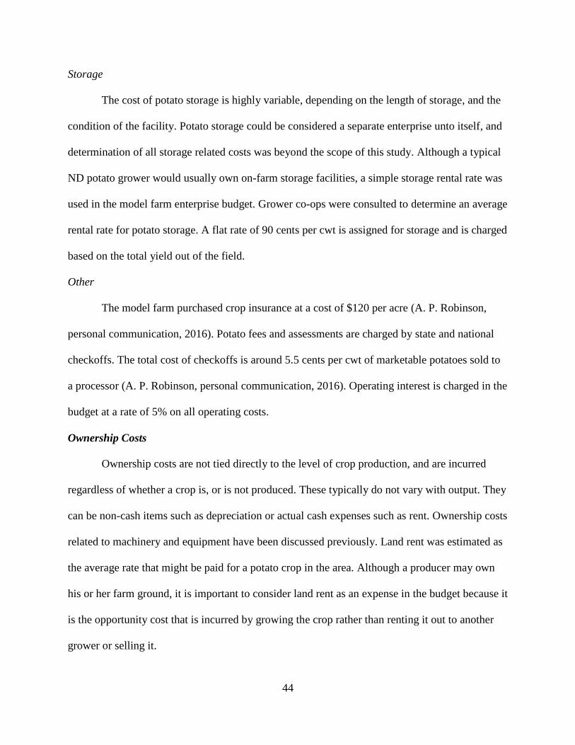
44
Storage
The cost of potato storage is highly variable, depending on the length of storage, and the
condition of the facility. Potato storage could be considered a separate enterprise unto itself, and
determination of all storage related costs was beyond the scope of this study. Although a typical
ND potato grower would usually own on-farm storage facilities, a simple storage rental rate was
used in the model farm enterprise budget. Grower co-ops were consulted to determine an average
rental rate for potato storage. A flat rate of 90 cents per cwt is assigned for storage and is charged
based on the total yield out of the field.
Other
The model farm purchased crop insurance at a cost of $120 per acre (A. P. Robinson,
personal communication, 2016). Potato fees and assessments are charged by state and national
checkoffs. The total cost of checkoffs is around 5.5 cents per cwt of marketable potatoes sold to
a processor (A. P. Robinson, personal communication, 2016). Operating interest is charged in the
budget at a rate of 5% on all operating costs.
Ownership Costs
Ownership costs are not tied directly to the level of crop production, and are incurred
regardless of whether a crop is, or is not produced. These typically do not vary with output. They
can be non-cash items such as depreciation or actual cash expenses such as rent. Ownership costs
related to machinery and equipment have been discussed previously. Land rent was estimated as
the average rate that might be paid for a potato crop in the area. Although a producer may own
his or her farm ground, it is important to consider land rent as an expense in the budget because it
is the opportunity cost that is incurred by growing the crop rather than renting it out to another
grower or selling it.

45
The management fee was also considered an ownership cost for the potato enterprise. The
management fee is the wage paid to the grower or manager for the management of the operation.
It is important to include a management wage, even when the owner is the one providing the
management, because it helps provide a more accurate assessment of the profitability of the
enterprise, and accounts for the opportunity cost of the grower’s time. In the model farm
enterprise budget, the management fee is set to be equivalent to 5% of the operating costs
(Patterson, 2013). It should be acknowledged that in practice, basing wages of management on
actual expenses may not be a wise strategy, because it takes away some of the incentive for
efficiency. This method was used simply to estimate a value that might be commensurate with
the scale of the operation. There is much less variability in input costs than in revenue and
therefore they provide a more stable basis for estimation of the management fee, for planning
purposes.
Stochastic Factors
The deterministic budget is an important tool for a potato grower to prepare, but the
reality is that they do not live in a world of fixed prices and conditions. Prices, weather, pest
pressure, and other factors shift often in unpredictable ways. Potato producers face uncertainty
and risk from many sources. Some sources of risk are more volatile than others. Stochastic
simulation was used to account for variability and risk. Stochastic values in the budget are
represented by statistical distributions that capture the range of probable values, rather than one
fixed value. The stochastic factors in this analysis are total yield and potato price. These were
selected not only for their volatility, but also for the weight of the effect that they can have on net
returns of the enterprise. Simulation strength and dependability is dependent upon the reliability
of the data from which distributions are defined. Defining these distributions in such a way that

46
they accurately model the variability of the input is a critical part of building the model and
setting up the simulation.
Price Data
Prices used in this budget may or may not reflect actual prices received by commercial
potato growers, due to differences in contracts or terminal markets. Processor contracts are often
complex, with discounts and premiums for tuber quality and condition. For simplicity in the
model, a single price is received for all tubers excluding culls and shrinkage of the crop in
storage.
Due to the extensive use of contracting, and differences in markets, reliable and recent
price data for processing potatoes can be difficult to obtain. Price distributions were derived
through a combination available historical data and expert opinion. Historical price data were
accessed from the United States Department of Agriculture (USDA) National Agricultural
Statistics Service (NASS). It is represented by the average price for processing potatoes in North
Dakota for the marketing year for the years of 1994 to 2009 (USDA, 2016). Based on observed
price distribution during this timeframe, the upward trend of nominal prices, expert opinion, and
grower consensus, the range of possible prices and the most likely price was estimated. The
RiskTriang function was used in the @Risk7 software package (Palisade Corporation, 2016) to
define the price within the stochastic budget with a minimum value of $7.50, a most likely value
of $8.50 and a maximum value of $9.50 per cwt Figure 8 illustrates the randomly sampled values
used in the simulation subject to the defined distribution.
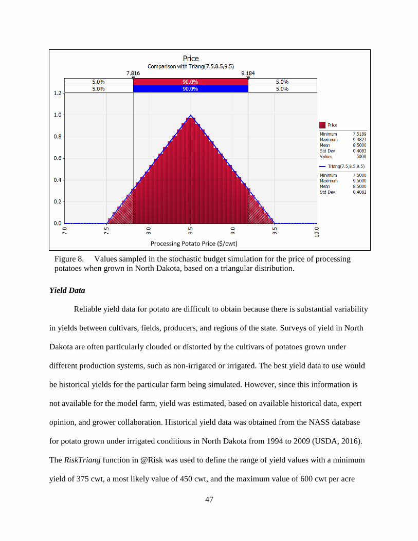
47
Yield Data
Reliable yield data for potato are difficult to obtain because there is substantial variability
in yields between cultivars, fields, producers, and regions of the state. Surveys of yield in North
Dakota are often particularly clouded or distorted by the cultivars of potatoes grown under
different production systems, such as non-irrigated or irrigated. The best yield data to use would
be historical yields for the particular farm being simulated. However, since this information is
not available for the model farm, yield was estimated, based on available historical data, expert
opinion, and grower collaboration. Historical yield data was obtained from the NASS database
for potato grown under irrigated conditions in North Dakota from 1994 to 2009 (USDA, 2016).
The RiskTriang function in @Risk was used to define the range of yield values with a minimum
yield of 375 cwt, a most likely value of 450 cwt, and the maximum value of 600 cwt per acre
Processing Potato Price ($/cwt)
Figure 8. Values sampled in the stochastic budget simulation for the price of processing
potatoes when grown in North Dakota, based on a triangular distribution.
48
(Figure 9). The randomly sampled yield values used in the simulation are depicted in Figure 8.
This is the total yield of the field, given in cwt per acre, before culls and storage shrink are
subtracted. It was estimated that, with fumigation, about 5% of the total yield would be culls, and
thus unmarketable. In addition, another 10% would be lost to shrinkage during storage. This
leaves approximately 85% of the total yield from the field that would be marketable. There is
some variability in this breakdown of total yield, and additional work should be done to consider
these percentages stochastically in the future. However, for the purpose of this analysis, only
total yield is treated stochastically.
Price-Yield Correlation
Historical price and yield data from the NASS database (USDA, 2016) were analyzed in
@Risk using the Batch Fit function to assess the possible relationship between the two variables
Irrigated Russet Potato Yield (cwt/ac)
Figure 9. Randomly sampled yield values used in the stochastic budget simulation for
irrigated russet potatoes in North Dakota, based on a triangular distribution.
49
and derive an appropriate correlation matrix. The two were found to be highly correlated with a
correlation coefficient of 0.788. The RiskCorrmat function was used in @Risk to correlate price
and yield sampling. RiskCorrmat allows for multivariate correlation by referencing distribution
functions to a correlation matrix (Palisade Corporation, 2016). This ensures that when price and
yield values are sampled for inputs in the simulation they are not treated independently.
Simulation
The stochastic simulation model is specified as
𝑁𝑅𝑖 = �̃�𝑖�̃�𝑖 − 𝑉𝐶 − 𝐹𝐶,
Where 𝑁𝑅𝑖 is the net return of simulation i, �̃�𝑖 and �̃�𝑖 are the simulated stochastic prices and
yields, VC is the variable cost, and FC is the fixed cost. The stochastic factors were defined by
their distribution functions, output for the simulation was specified as net returns above total cost
per acre. @Risk was used to simulate the model with 5,000 iterations, yielding 5,000 unique net
returns based on the random sampling of the stochastic inputs.
Results and Discussion
It is common for farming operations to prepare a pro forma budget when planning for the
upcoming year. These budgets are nearly always deterministic in nature; however, there are a
number of unknown and risky factors that make up some of the budget inputs. A deterministic
budget only captures a single snapshot of a possible outcome, when in fact, there is a very wide
range of possible outcomes due to many factors outside of the grower’s control. This variability
is particularly profound in potato production. Initial preparation of a deterministic budget yielded
a net return of $217 per acre, or $434,000 for the two thousand acre potato enterprise on the
model farm. If a producer is not aware of the level of risk that exists in the enterprise he or she
may develop a distorted view of their actual position. If decisions are made based largely on faith

50
in the picture presented by the deterministic budget, without a means of quantifying and planning
for the risk and level of deviation from the budget outcome, producers may face a financial
catastrophe, or overlook a great opportunity.
Distribution of Simulated Net Returns
Most producers likely understand that there is a certain amount of risk and variability
involved in growing and selling potatoes. The results obtained from the stochastic simulation
aids understanding of the level of the risk involved. The simulation helps us understand the best
and worse-case scenarios, and their probability of occurrence. The outputs (net returns) of each
of the 5,000 iterations in the simulation were compiled into a histogram by @Risk, allowing for
easy analysis of the results. Individual producers may have differing input costs, thus the shape
of the output curve of the simulation is perhaps more important than the actual values derived.
The shape and spread of the curve is determined by the stochastic inputs of price and yield. Input
costs were treated as deterministic in this simulation, thus a producer with lower or higher input
costs than the ones in this simulation may simply shift the curve to the left or the right by the
amount of the difference in cost. Figure 10 shows the distribution of the simulated outcomes in a
histogram. The mean net return in the simulation was $384 per acre. The standard deviation of
the output was $430 per acre. In other words, net returns per acre will lie between -$47 and $813
per acre, approximately two years out of three (plus or minus one standard deviation). The range
of possible returns that lie within one standard deviation of the mean varies by $1.72 million for
the potato enterprise on the model farm. Standard deviation provides a useful value for
understanding the level of variability, which is often closely associated with the level of risk
(Palisade Corporation, 2016). The higher the standard deviation, the greater the variability that
exists in the outcome. This can be a useful value to compare the enterprise with other investment

51
opportunities, when discussing risk management. In the simulation, 20.4% of the iterations
yielded a negative net return. The implication of this, is that in order for a potato producer to
ensure their longevity in the enterprise, they must position the business such that it may
withstand losing money approximately one year in five. Potato producers may feel optimistic
since the distribution is skewed to the right, indicating that the potential for the highest returns is
greater than the risk of the most substantial losses. Net returns observed in the simulation ranged
from a loss of $551 per acre, or $1.10 million for the enterprise, to gains of $1,616 per acre, or
$3.23 million for the entire enterprise.
Net Returns ($/ac)
Figure 10. Probability density of simulated net returns, in dollars per acre, of irrigated
russet potatoes grown in North Dakota for the processing market.

52
BestFit was used to fit a distribution to the output results for net returns; the beta general
distribution was found to be the best according to the five goodness-of-fit statistics (Palisade
Corporation, 2016). Often a farmer might expect his or her returns to be somewhat normally
distributed. It appears that an assumption of normally distributed returns would actually
overestimate potential losses, as seen in the left tail of the distribution (Figure 11). A producer
acting on the assumption of normality, rather than on the basis of beta general distributed returns,
is likely to take a slightly more risk averse position than intended. The normal distribution has
slightly longer tails, particularly the lower tail, so the magnitude of potential losses may be
slightly overestimated with normally distributed returns.
Net Returns ($/ac)
Figure 11. The best fit (beta general) and normal distributions, fit to the simulated net
returns ($/ac) for irrigated russet potatoes grown in North Dakota.

53
A Wheat Comparison
In order to put the range of simulated potato returns into perspective, a similar, simplified
analysis was conducted on hard red spring wheat. Wheat was chosen because it is another crop
grown by the model farm and is typical in the crop rotation, with potatoes, in North Dakota. An
enterprise budget for wheat was obtained from the North Dakota State University Extension
Service (Swenson and Haugen, 2015). Price and yield were defined stochastically in the
enterprise budget with normal distributions. Ten years of data was collected from the USDA
(2016) NASS quick stats, in order to derive a mean and standard deviation for the price and yield
of hard red spring wheat in ND.
Simulated net returns for wheat where much more tightly clustered around the mean than
the net returns for potato (Figure 12). Wheat did not have the large chance of substantial losses
that were present in potato; however, there was not the same possibility for large returns on the
upper end either. Values representing the greatest 5% of losses in wheat are surpassed by potato
35% of the time. Conversely, values representing the most profitable 5% of years in wheat, were
exceeded by potato nearly half of the time (45%). The difference in the volatility of net returns is
apparent in the standard deviation. The standard deviation for potato net returns is $384.4 per
acre, while the standard deviation for the net returns of wheat is $86.2 per acre. The value of one
standard deviation is $149,100 greater for the 500 acre potato enterprise than for the 500 acre
wheat enterprise.

54
Magnitude of Input Effect on Net Returns
The tornado graph represents the magnitude of the effect of each of the stochastic inputs
(price and yield) on net returns (Figure 13). The variability in price and yield, each have a nearly
equivalent potential to affect the net returns of the potato enterprise; however, yield has a slightly
larger ability to impact net returns than does yield, particularly on the upper end. This near-
equivalence, allows the grower to pursue whatever risk management tools may be available
knowing that management of either price or yield risk could efficiently decrease risk to the
enterprise. There may be a slight relative advantage to controlling yield risk, but the difference is
too small to say definitively. Price risk tools would be those things such as contracts or direct
marketing, while yield risks could be managed with fumigation, scouting, efficient irrigation, and
other crop health management strategies.
Net Returns ($/ac)
Wheat Returns
Potato Returns
Figure 12. Overlaid probability density of net returns for hard red spring wheat and
irrigated russet potato.

55
Conclusion
It is a generally accepted notion that potato production is a risky enterprise; however, this
is a somewhat subjective statement and does not provide any indication of the level of risk
involved or how it may compare with another enterprise. A deterministic enterprise budget is an
important starting point in seeking to understand what is at stake financially; however, it only
provides a snapshot of one possible outcome. In reality, certain elements of the budget are
variable and unpredictable, thus the returns expected are variable and unpredictable. Stochastic
(or Monte Carlo) budgeting uses simulation to account for the variability, or risk, within the
budget. Risky elements are considered as ranges of possible values rather than fixed amounts.
Price and yield are some of the most unpredictable, or risky, budget components with the
greatest effect on net returns. Ranges of values for both price and yield were derived by a
Net Returns ($/ac)
Figure 13. Tornado graph of the magnitude of the effect of each stochastic input (price and
yield) on irrigated russet potato net returns ($/acre) in North Dakota.
56
combination of historical data from North Dakota and expert opinion. The price for russet
processing potatoes ranged from $7.50 to $9.50 per cwt. Yield values ranged from 375 to 600
cwt per acre.
Simulation of the irrigated potato enterprise on the model farm yielded a positive mean
net return of $384 per acre, but also had a somewhat high standard deviation for net returns,
making it difficult to predict positive returns consistently from year to year. Variability in price
and yield have the potential to expose the enterprise to nearly equivalent levels of risk to net
returns. The authors do not attempt to classify irrigated processing potato production as strictly
low or high risk; however, these values provide a metric with which to measure the enterprise
against others where resources might be devoted, to form a relative ranking of risk. Every
decision maker has unique risk preferences based on their position and appetite for risk.
Individual preferences for each party invested in the success of the enterprise should be
understood and accounted for by the decision maker seeking to manage risk and maximize
returns.
Literature Cited
Amvac Chemical Corporation. 2015. Vapam® HL™ soil fumigant product label. EPA Reg. No.
5481-468 2017.
Bethke, P. C. et al. 2014. History and origin of Russet Burbank (Netted Gem) a sport of
Burbank. Am. J. Potato Res. 91:594-609.
Bogash, S. M., W. J. Lamont Jr., R. M. Harsh, and L. F. Kime. 2013. Potato Production. Penn
State Extension. Code UA360.

57
Bohl, W. H. and S. B. Johnson (Eds.). 2010. Commercial potato production in North America.
The Potato Association of America Handbook. Second Revision of American Potato
Journal Supplement Vol. 57.
Edwards, W. 2015. Estimating farm machinery costs. Ag Decision Maker, File A3-29. Iowa
State University Extension and Outreach.
Galinato, S. P., and P. R. Tozer. 2016. 2015 Costs estimates of producing fresh and processing
potatoes in Washington. Washington State University Extension (TB14).
Kazmierczak, R. F. and P. Soto. 2001. Stochastic economic variables and their effect on net
returns to channel catfish production. Aquac. Econ. Manag., 5:1-2, 15-36.
Khakbazan M., R. Carew, S. L. Scott, P. Chiang, H. C. Block, C. Robins, O. N. Durunna, and J.
Huang. 2014. Economic analysis and stochastic simulation of alternative beef calving and
feeding systems in western Canada. Can. Anim. Sci 94:299-311.
Knight F. H. 1921. Risk, Uncertainty, and Profit. Houghton Mifflin. Boston and New York.
Kwak, Y. H. and L. Ingall. 2007. Exploring Monte Carlo simulation applications for project
management. Risk Management 9(1):44-45.
Myers, R. J., R. J. Sexton, W. G. Tomek. 2010. A century of research on agricultural markets.
Am. J. Agric. Econ. 92(2): 376-402.
NDAWN (North Dakota Agricultural Weather Network). 2017. NWS Monthly Normal Weather
Data. Retrieved from https://ndawn.ndsu.nodak.edu/weather-data-nws-monthly-
normals.html.
Palisade Corporation. 2016. @Risk 7.5.0. Palisade Corporation, Ithaca, NY.
58
Patterson, P. E. 2013. Eastern Idaho Southern Region: Bannock, Bingham, & Power Counties,
Russet Burbank Potatoes: Production and Storage Costs. University of Idaho 2013 Costs
and Returns Estimate EBB4-Po-13.
Riley, W. B. and K. V. Chow. 1992. Asset allocation and individual risk aversion. Financ. Anal.
J. 48(6): 32-37.
Robinson, L.J. and P.J. Barry. 1986. The Competitive Firm’s Response to Risk. Macmillan
Publishers pp. 11-15.
Swenson, A. and R. Haugen. 2015. Projected 2016 Crop Budgets, North Valley North Dakota.
North Dakota State University Extension Service, EC1656.
USDA (United States Department of Agriculture). 2016. National Agricultural Statistical Service
(NASS), Quick Stats. Retrieved from https://quickstats.nass.usda.gov/.

59
FUMIGATION COST AND BREAK-EVEN ANALYSIS
Abstract
Soil fumigants are an important management tool in potato against certain yield limiting
diseases; however, they are often among the highest single input costs for the potato crop. It is
important for a producer to carefully evaluate the minimum benefit that must be realized in order
justify incurring the cost of treatment. Fumigation break-even is a function of three variables,
yield increase, increase in percent yield marketable, and market price. Yield increase required to
break even has an inverse relationship to market price. Differences in the marketable yield rate
due to fumigation, become less significant as yield increases due to fumigation become greater.
The significance of differences in the marketable yield rate among products, decreases as total
yield increases rise. Finally, the relative break even yield increase required will be lower for the
scenario with the higher pre-fumigation yield potential, regardless of market price.
Introduction
Research indicates that significant total yield improvements, as well as improvements in
the marketable yield percentage, may be gained with both metam sodium (Pasche et al., 2014)
and chloropicrin fumigation (Hutchinson, 2005). Fumigation, if undertaken, may be among some
of the largest single expenses to the potato enterprise. According to the NDSU model farm
budget for irrigated russet potatoes, storage costs are the largest single expense, at nearly 18% of
total operating costs, and fumigation is second, at approximately 16% of operating costs (see
Table A7). The next greatest costs are fertilizer and seed, at 15% and 11% of operating costs,
respectively (Table A7). A producer must carefully evaluate the benefits to yield and quality,
gained from fumigation, in order to decide if they outweigh the high cost of fumigation. The

60
objective of this chapter is to look at the combination of minimum criteria (break-even point),
which must be met in order for fumigation to be economically feasible.
One of the most significant yield limiting factors faced by producers, especially in fields
with a long history of potato production, is known as potato early dying (PED), also known as
Verticillium wilt or early maturity wilt (Powelson and Rowe, 1993). This problem is of particular
significance in the Red River Valley of North Dakota and Minnesota, and in Idaho where PED
has developed slowly over many years (Powelson and Rowe, 1993).
Potato early dying is a common fungal disease of potato caused by one of two soil borne
fungi, Verticillium albo-atrum or Verticillium dahliae (Wiggins 2002). Potato early dying thrives
in warm temperatures. The optimal growth temperature for potatoes ranges from 65 to 68 F (18
to 20 C) while the optimal range for V. dahlia is 70 to 80 F (21 to 27 C) (Powelson and Rowe,
1993). Potato early dying causes premature senescence of the potato plant, four to six weeks
earlier than normal (Kleinkopf et al. 2003). This can have a tremendous effect on a potato
producer because it takes place during the important tuber bulking period of growth. During the
bulking stage, Russet Burbank potatoes will increase yield by an average of 6.5 cwt/ac/day (729
kg/ha/day) (Kleinkopf et al. 2003). Premature senescence can lead to a significant reduction in
tuber size and total marketable yield. Reductions in yield of moderately affected fields can be 10
to 15%; severely diseased fields can have yields reduced by 30 to 50% (Rowe and Powelson,
2002).
Verticillium wilt is arguably the most economically damaging disease to the potato
industry in the United States when considering loss of yield and quality, and cost of control
(Gudmestad et al. 2007). The recognition of this growing problem has been complicated in
recent decades due to improved cultivars and cultural practices that have led to increased yields

61
(Powelson and Rowe, 1993). With these improvements the reduction in yield due to PED is less
apparent, as overall yields have continued to rise. The true cost could be thought of as the
potential for increased yield that has gone unrealized (Powelson and Rowe, 1993).
Management of PED
Cultivar selection is one of the standard recommendations for disease control and
management in any crop. This is probably one of the best and most sustainable means of disease
control; however, disease-resistant varieties often are not available in many crops, including
potatoes. In fact, very few potato cultivars grown in the United States are more than moderately
disease resistant (Secor and Gudmestad, 1999). Even when disease-resistant cultivars exist, they
may not be suitable for the intended end use, such as chipping or baking (Secor and Gudmestad,
1999). Tillage practices are also a component of management of PED. Moldboard plowing helps
redistribute the soil strata, burying the top few inches where the majority of the Verticillium
propagules are found. A crop rotation allowing three or more years between potato crops also
will help mitigate PED (Gudmestad et al., 2007). Fields cropped to potatoes with a rotation of
two years or less between potato crops have been found to have two to four times greater
Verticillium populations, than fields with longer rotations (Gudmestad et al., 2007).
The primary industry standard practice for controlling PED for the past several decades
has been the application of metam-sodium (Rowe and Powelson, 2002). Metam sodium is a soil
fumigant that is applied as a liquid and must volatize in order to permeate the soil profile
(Gudmestad et al., 2007). Chloropicrin is another chemical used as a pre-plant soil fumigant to
control soil-borne pests. It has been used agriculturally as a soil fumigant since 1920 (Pegg,
1984), but use in potatoes in the Upper Midwest is relatively new (A. P. Robinson, personal
communication, 2016). The strong fungal control properties of chloropicrin are anticipated to
62
improve tuber yield and quality by reducing Verticillium populations in the soil (Hutchinson,
2005). Chloropicrin was first used in strawberry production in California to control Verticillium
wilt (Duniway, 2002). Mixtures of chloropicrin and methyl bromide have become standard
applications for strawberries in California, and studies have shown yield increases of 44 to 85%
as a result of fumigation (Duniway, 2002). Chloropicrin has also been used in nursery plants,
peppers, tomatoes, and other crops. Historically, it has been shank applied or, more recently, as a
drip application to the bed (Martin, 2003). The initial cost associated with chloropicrin treatment
is higher, relative to that of metam sodium; one would need to realize a greater increase in yield
or quality to adopt its use.
No matter what product or application method is employed, fumigation can be one of the
single largest expenses in a potato enterprise budget. The decision to fumigate should be made
carefully, considering all the costs and risks associated. Fumigation can be an effective tool for
managing yield risk, but there is also the associated financial risk, that resources will be
expended on treatment without realizing the full anticipated benefit. There are studies that look
at fumigants and their effectiveness against their targets; however, there is little discussion of the
cost effectiveness of these measures. The objective of this study was to identify the various
combinations of yield and quality improvements that would need to be realized, in order for
fumigation to be economically advantageous, depending on the market price of potatoes.
Materials and Methods
Fumigation Cost
Based on input from industry representatives, the custom application cost to inject metam
sodium with deep shank tillage was estimated to be $60 per acre (Table A7). The rate of
application used in this analysis was 50 gallons per acre (Amvac Chemical Corporation, 2015).

63
At a cost of $6 per gallon, the product cost is $300 per acre (Table A7). The total cost of
fumigation for metam sodium is $360 per acre. The custom application rate for chloropicrin was
estimated to be $35 per acre. The rate of application used was 100 pounds per acre (A. P.
Robinson, personal communication, 2016). The cost is $4 per pound. The total fumigation cost
of chloropicrin was $435 per acre.
Break-Even Discussion
This chapter does not attempt to establish which product yields superior net returns but
rather to provide a simple means of analysis and comparison that producers may employ in
understanding their own results and expectations. It demonstrates what variety of price and yield
combinations would need to be expected in order to break-even with the additional cost of a
fumigation. The examples shown are “what if” scenarios and not necessarily intended to
represent actual results. This discussion focuses on two types of fumigation, but this concept
could be applied to many of the production input decisions that are made by a potato producer.
There are three ways for a potato enterprise to increase revenue to pay for additional
expenses incurred—a higher volume of tubers must be sold, marketable quality must improve, or
tubers must be sold for more money. The three primary variables in consideration for this
discussion are increase in total yield, increase in the marketable yield rate, and the price paid to
the grower. The increase in yield required to break-even is a downward sloping curve with
respect to increasing prices, as illustrated in Figure 14. This is an example of a metam sodium
application with an assumption of a 7% increase in marketable yield, based on a 350 cwt per acre
yield without fumigation. The fumigation break-even yield increase curve was generated with a
range of price values inserted in the following formula:
∆𝑌 =𝐶 − 𝑃𝑌∆𝑀
𝑃(∆𝑀 + 𝑀)

64
Where: ΔY = Change in yield required to break even on the application
C = Cost of fumigation
P = Potato price
Y = Total yield without fumigation
M = Percent marketable tubers without fumigation
ΔM = Increase in percent marketable tubers due to fumigation
Considering the same information in a different way, Table A13 provides the minimum
market conditions that would need to be met in order to break even on the fumigation based on
the range of potential yield increases and improvements in the marketable yield rate realized due
to fumigation. The table values were derived with the following formula:
𝑃 =𝐶
𝑌∆𝑀 + ∆𝑌(𝑀 + ∆𝑀)
Where: P = Potato price required to break even on fumigation
Greater increases in yield or marketable yield rate are necessary to offset the cost of fumigation
when potato prices are low. Figure 15 shows a wide separation in break-even prices, among three
marketable yield rate increases, when total yield increases are low; however, the separation
narrows rapidly as the yield increase gained from fumigation grows. The implication of this is
0
10
20
30
40
50
60
70
80
90
4 4.5 5 5.5 6 6.5 7 7.5 8 8.5 9 9.5 10 10.5 11 11.5 12
Yie
ld i
ncr
ease
(cw
t./a
cre)
Price ($/cwt.)
Figure 14. Example curve of yield increase needed to break even on metam sodium
application. Based on a 350 cwt per acre total yield without fumigation, assumes 76%
marketable yield rate without fumigation, and assumes a 7% increase in the marketable
yield rate due to fumigation. Fumigation cost of $360 per acre
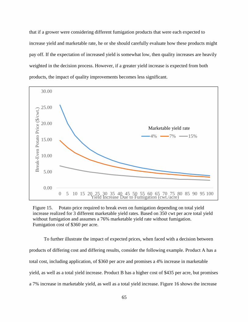
65
that if a grower were considering different fumigation products that were each expected to
increase yield and marketable rate, he or she should carefully evaluate how these products might
pay off. If the expectation of increased yield is somewhat low, then quality increases are heavily
weighted in the decision process. However, if a greater yield increase is expected from both
products, the impact of quality improvements becomes less significant.
To further illustrate the impact of expected prices, when faced with a decision between
products of differing cost and differing results, consider the following example. Product A has a
total cost, including application, of $360 per acre and promises a 4% increase in marketable
yield, as well as a total yield increase. Product B has a higher cost of $435 per acre, but promises
a 7% increase in marketable yield, as well as a total yield increase. Figure 16 shows the increase
0.00
5.00
10.00
15.00
20.00
25.00
30.00
0 5 10 15 20 25 30 35 40 45 50 55 60 65 70 75 80 85 90 95 100
Bre
ak-E
ven
Pota
to P
rice
($/c
wt.
)
Yield Increase Due to Fumigation (cwt./acre)
4% 7% 15%
Marketable yield rate
Figure 15. Potato price required to break even on fumigation depending on total yield
increase realized for 3 different marketable yield rates. Based on 350 cwt per acre total yield
without fumigation and assumes a 76% marketable yield rate without fumigation.
Fumigation cost of $360 per acre.

66
in total yield that would need to be attained for each of these two products to break even at a
range of prices. If prices are expected to be low, the risk-averse preferred decision would be to
employ the cheaper product, assuming both products increased total yield equally. However, as
prices increase, these curves intersect, and the more expensive product B becomes more
favorable, keeping all else constant.
The level of yield a potato operation is able to achieve without fumigation is also an
important factor to take into consideration when making the decision to fumigate. Consider two
potato operations, one is growing irrigated russet potatoes with an average total yield of 350 cwt
per acre, and the other is growing non-irrigated red potatoes with an average total yield of 190
cwt per acre. Assume that each enterprise has a 76% marketable rate without fumigation. The red
potato grower will need to see a greater increase in yield to pay for the fumigation at any price
level. This is because fumigation is a cost incurred by the acre. For the irrigated grower, the per-
10
20
30
40
50
60
5 5.5 6 6.5 7 7.5 8 8.5 9 9.5 10 10.5 11 11.5 12
Addit
ional
yie
ld n
eeded
to b
reak
even
(cw
t./a
cre)
Potato Price ($/cwt)
Product A--4% increase in
marketables
Product B--7% increase in
marketables
Figure 16. Yield increase needed to break even, subject to market price, for
two different fumigant products with differing increases in marketable yield rate.
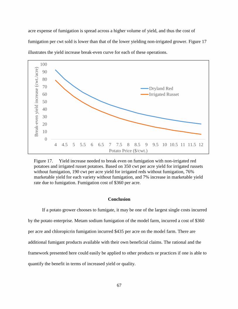
67
acre expense of fumigation is spread across a higher volume of yield, and thus the cost of
fumigation per cwt sold is lower than that of the lower yielding non-irrigated grower. Figure 17
illustrates the yield increase break-even curve for each of these operations.
Conclusion
If a potato grower chooses to fumigate, it may be one of the largest single costs incurred
by the potato enterprise. Metam sodium fumigation of the model farm, incurred a cost of $360
per acre and chloropicrin fumigation incurred $435 per acre on the model farm. There are
additional fumigant products available with their own beneficial claims. The rational and the
framework presented here could easily be applied to other products or practices if one is able to
quantify the benefit in terms of increased yield or quality.
0
10
20
30
40
50
60
70
80
90
100
4 4.5 5 5.5 6 6.5 7 7.5 8 8.5 9 9.5 10 10.5 11 11.5 12
Bre
ak-e
ven
yie
ld i
ncr
ease
(cw
t./a
cre)
Potato Price ($/cwt.)
Dryland Red
Irrigated Russet
Figure 17. Yield increase needed to break even on fumigation with non-irrigated red
potatoes and irrigated russet potatoes. Based on 350 cwt per acre yield for irrigated russets
without fumigation, 190 cwt per acre yield for irrigated reds without fumigation, 76%
marketable yield for each variety without fumigation, and 7% increase in marketable yield
rate due to fumigation. Fumigation cost of $360 per acre.
68
The authors have not attempted to establish a superior product, but rather sought to lay
out the conditions which would need to be met in order to break even on fumigation application.
The three variables considered in this analysis were market price, increase in total yield, and
increase in the marketable yield rate. As the market price of potatoes increases, the break-even
curve is downward sloping, meaning that at higher market prices it takes less of an increase in
yield or quality to pay for fumigation. While this may seem like an obvious observation, it is
important for the farm to take the time to consider exactly where they fall on the curve. From a
risk management perspective, a reasonable strategy would be to seek to minimize costs when
prices are low, even if some yield is sacrificed, and to strive to maximize yields when prices are
expected to be high, possibly to the point of incurring significant additional cost. There are times
when it may not be possible to determine the best product to apply even when the increase in
yield and quality are known. The break-even curves of two products of different costs, with
different increases in quality may intersect, depending on the market price that will be received.
A system with a higher before-fumigation yield will always have a lower break-even point than
one with a lower yield, because the cost of application is spread out among more units of sale.
In a real-world application there are several combinations of variables that interact with
one another in different ways to affect the outcome of a particular decision. One must continually
evaluate these considerations as they change, based on conditions and market expectations.
Literature Cited
Amvac Chemical Corporation. 2015. Vapam® HL™ soil fumigant product label. EPA Reg. No.
5481-468 2017.
Duniway, J.M. 2002. Status of chemical alternatives to methyl bromide for pre-plant fumigation
of soil. Phytopathol. 92:1337-1343.

69
Gudmestad, N.C., R.J. Taylor, and J.S. Pasche. 2007. Management of soilbourne diseases of
potato. Australas. Plant Pathol. 36(2):109-115.
Hutchinson, C.M. 2005. Evaluation of chloropicrin soil fumigation programs for potato (solanum
tuberosum) production. Proc. Fla. State Hort. Soc. 118:129-131.
Kleinkopf, G.E., T.L. Brandt, and N. Olsen. 2003. Physiology of tuber bulking. Presented at
Idaho Potato Conference. January 23, 2003.
Martin, F.N. 2003. Development of alternative strategies for management of soilborne pathogens
currently controlled with methyl bromide. Ann. Rev. Phytopathol. 41:325-350.
Pasche, J.S., R.J. Taylor, N. L. David, N.C. Gudmestad. 2014. Effect of soil temperature,
injection depth, and metam sodium rate on the management of Verticillium wilt of
potato. Am. J. Potato Res. 91: 277.
Pegg, G.F. 1984. The impact of Verticillium diseases in agriculture. Phytopathologia
Mediterranea 23(2/3):176-192.
Powelson, M.L., and R.C. Rowe. 1993. Biology and management of early dying of potatoes.
Annu. Rev. Phytopathol. 31:111-126.
Rowe, R.C., and M.L. Powelson. 2002. Potato early dying: management challenges in a
changing production environment. Plant Dis. 86:1184-1193.
Secor, G.A., and N.C. Gudmestad. 1999. Managing fungal diseases of potato. Can. J. Plant
Pathol. 21(3): 213-221.
Wiggens, E. 2002. Verticillium wilt of tomatoes and potatoes. University of Minnesota,
Extension, P261V. Retrieved from http://www.extension.umn.edu/garden/yard-
garden/vegetables/Verticillium-wilt-of-tomatoes-and-potatoes/.

70
APPENDIX
Table A1. NDSU model farm budget for non-irrigated red potato production.
Quantity
per Acre Unit
Price
per
Unit
Value or
cost/acre
Value or
cost/cwt
GROSS RETURNS --------------------$--------------------
Total Yield 186 cwt 2709.7
5 19.22
A (marketable) 75
% 106 cwt 16.31 1724.4
3
B 20
% 28 cwt 23.96 675.48
C 5% 7 cwt 43.96 309.85
Culls 12
%
Shrinkage 12
%
% Marketable 76
%
TOTAL GROSS RETURNS 2709.7
5 19.22
OPERATING INPUTS
Seed 324.00 2.30
G3 Red Norland Seed 24 cwt 12.00 288.00
Seed Freight 24 cwt 1.00 24.00
Seed Cutting 24 cwt 0.50 12.00
Fertilizer Refer to Table A2 172.01 1.22
Pesticides 170.54 1.21
Herbicide Refer to Table A3 49.22
Insecticide for an itemized breakdown 3.74
Fungicide of pesticide costs 85.93
Desiccant 31.65
Custom 81.50 0.58
Custom Fertilize 1 app 6.50 6.50
Consultants/Soil Testing 1 acre 10.00 10.00
Custom Spray 10 spray 6.50 65.00
Machinery 150.62 1.07
Fuel--Gas 3.1 gal 2.40 7.43
Fuel--Red Diesel 13.7 gal 2.00 27.42
Fuel--Road Diesel 6.2 gal 2.60 16.12
Lube Refer to Table A5 for 7.65
Machinery Repair itemized lube and repair 92.00
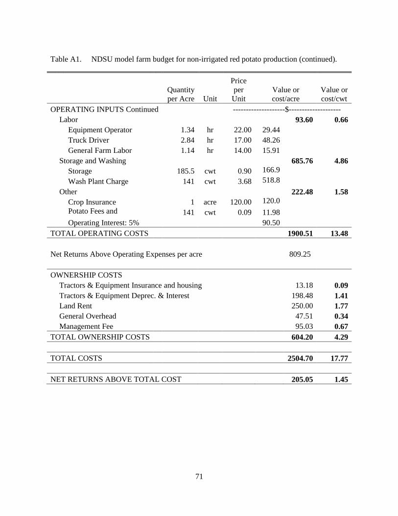
71
Table A1. NDSU model farm budget for non-irrigated red potato production (continued).
Quantity
per Acre Unit
Price
per
Unit
Value or
cost/acre
Value or
cost/cwt
OPERATING INPUTS Continued --------------------$--------------------
Labor 93.60 0.66
Equipment Operator 1.34 hr 22.00 29.44
Truck Driver 2.84 hr 17.00 48.26
General Farm Labor 1.14 hr 14.00 15.91
Storage and Washing 685.76 4.86
Storage 185.5 cwt 0.90 166.9
5
Wash Plant Charge 141 cwt 3.68 518.8
1
Other 222.48 1.58
Crop Insurance 1 acre 120.00 120.0
0
Potato Fees and
Assessments 141 cwt 0.09 11.98
Operating Interest: 5% 90.50
TOTAL OPERATING COSTS 1900.51 13.48
Net Returns Above Operating Expenses per acre 809.25
OWNERSHIP COSTS
Tractors & Equipment Insurance and housing 13.18 0.09
Tractors & Equipment Deprec. & Interest 198.48 1.41
Land Rent 250.00 1.77
General Overhead 47.51 0.34
Management Fee 95.03 0.67
TOTAL OWNERSHIP COSTS 604.20 4.29
TOTAL COSTS 2504.70 17.77
NET RETURNS ABOVE TOTAL COST 205.05 1.45
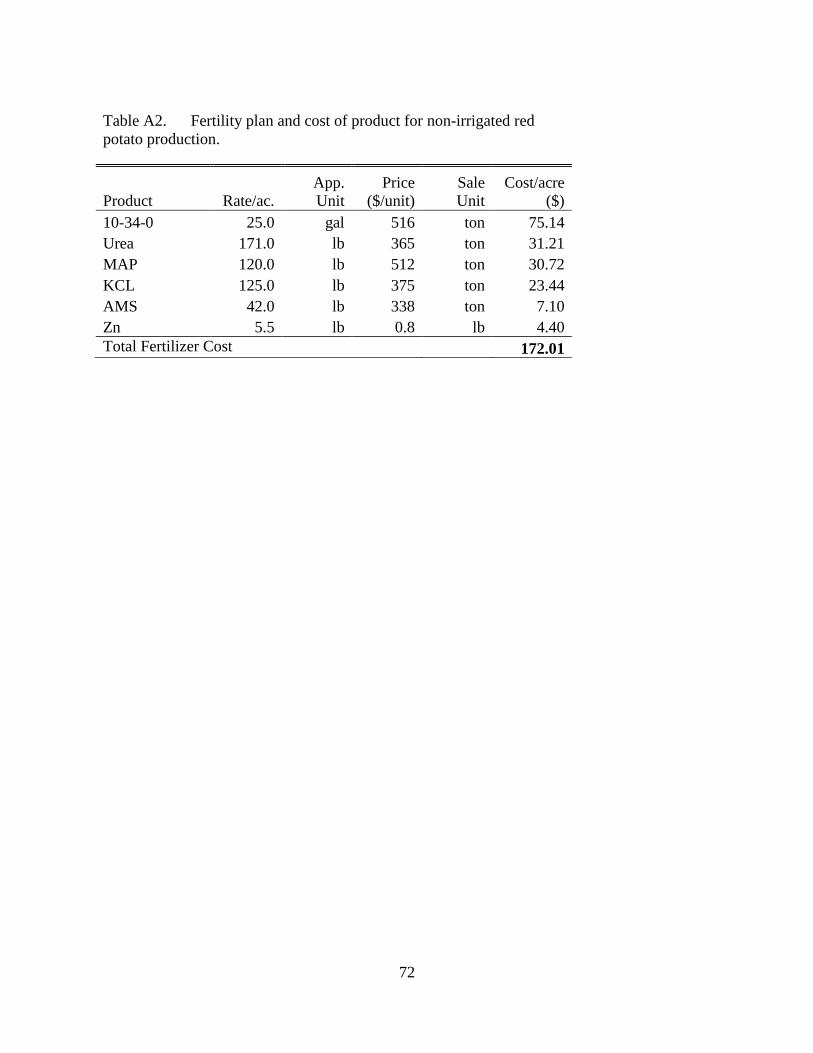
72
Table A2. Fertility plan and cost of product for non-irrigated red
potato production.
Product Rate/ac.
App.
Unit
Price
($/unit)
Sale
Unit
Cost/acre
($)
10-34-0 25.0 gal 516 ton 75.14
Urea 171.0 lb 365 ton 31.21
MAP 120.0 lb 512 ton 30.72
KCL 125.0 lb 375 ton 23.44
AMS 42.0 lb 338 ton 7.10
Zn 5.5 lb 0.8 lb 4.40
Total Fertilizer Cost
172.01

73
Table A3. Pesticide application rates and cost of product for non-irrigated
red potato production.
Product Rate/ac.
app.
Unit
Price
$/unit
sale
Unit
Cost/acre
($)
Herbicide
Pre-emergent
Dual Magnum 1.5 pt 120 gal 22.50
Prowl H2O 2.7 pt 50 gal 16.72
Metribuzin 0.5 lb 20 lb 10.00
Post-emergent
MH-30 1 gal 15 gal 15.00
2,4-D 2.3 oz 28 gal 0.50
2,4-D 2.3 oz 28 gal 0.50
Total herbicide cost 49.22
Insecticide
Admire Pro 8.7 oz 55 gal 3.74
Total insecticide cost 3.74
Fungicide
Seed
Emesto Silver 0.31 oz/cwt 325 gal 18.89
Quadris 8.7 oz 190 gal 12.91
Foliar
Echo 720 0.75 pt 30 gal 2.81
Koverall 2 lb 3 lb 6.00
Echo 720 1.5 pt 30 gal 5.63
Koverall 2 lb 3 lb 6.00
Luna Tranquility 11.2 oz 385 gal 33.69
Total fungicide cost
85.93
Desiccant
Reglone 1 pt 105 gal 13.13
R11 adjuvant 0.8 pt 27 gal 2.70
Reglone 1 pt 105 gal 13.13
R11 adjuvant 0.8 pt 27 gal 2.70
Total desiccant cost 31.65

74
Table A4. Whole farm equipment overhead costs for non-irrigated red potato production.
Capital Recovery Insurance & Housing Potato
Equipment New cost
Years
life
Salvage
value
Farm
total
Potato
portion
Farm
total
Potato
portion
overhead
per acre
Pickup 1 - 3/4 ton 45,000 5 14,000 7,861 3,144 295 118 6.52
Pickup 2 - 3/4 ton 45,000 5 14,000 7,861 3,144 295 118 6.52
Pickup 3 - 3/4 ton 45,000 5 14,000 7,861 3,144 295 118 6.52
Tractor 1 - 260hp MFWD 301,000 12 84,280 28,703 12,757 1,926 856 27.23
Tractor 2 - 350hp track 360,000 12 100,800 34,330 13,732 2,304 922 29.31
Tractor 3 - 225hp MFWD 225,000 12 63,000 21,456 10,728 1,440 720 22.90
Potato Planter 6-Row 75,000 25 - 5,325 5,325 375 375 11.40
Potato Hiller 6-Row 25,000 30 - 1,625 1,625 125 125 3.50
Potato Harvester 4-Row 160,000 20 15,000 12,350 12,350 875 875 26.45
Harvester #2 - 4-Row 160,000 20 15,000 12,350 12,350 875 875 26.45
Truck 1 - Tandem axle 105,000 20 7,000 8,190 4,095 560 280 8.75
Truck 2 - Tandem axle 105,000 20 7,000 8,190 4,095 560 280 8.75
Truck 3 - Tandem axle 105,000 20 7,000 8,190 4,095 560 280 8.75
Truck 4 - Tandem axle 105,000 20 7,000 8,190 4,095 560 280 8.75
Truck 5 - Tandem axle 105,000 20 7,000 8,190 4,095 560 280 8.75
Truck 6 - Tandem axle 105,000 20 7,000 8,190 4,095 560 280 8.75
Truck 7 - Tandem axle 105,000 20 7,000 8,190 4,095 560 280 8.75
Truck 8 - Tandem axle 105,000 20 7,000 8,190 4,095 560 280 8.75
Chisel plow - 37ft 49,000 20 7,840 3,685 921 284 71 1.98
Tandem Disk - 30ft fold 54,000 20 8,640 4,061 1,015 313 78 2.19
Dump truck 30,000 20 2,000 2,340 2,340 160 160 5.00
Fuel Truck 50,000 20 3,000 3,910 1,564 265 106 3.34
Service Truck 40,000 20 3,000 3,110 1,244 215 86 2.66
Totals 2,504,000 400,560 222,348 118,144 14,523 7,843 251.98
84% of New Cost* 2,103,360 336,470 186,772 99,241 12,199 6,588 211.66
*Used to reflect a mix of new and used equipment (Patterson, 2013)
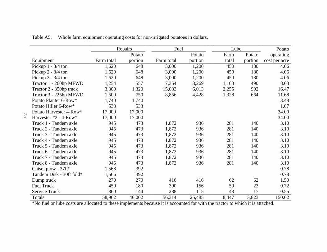
75
Table A5. Whole farm equipment operating costs for non-irrigated potatoes in dollars.
Repairs Fuel Lube Potato
operating
cost per acre Equipment Farm total
Potato
portion Farm total
Potato
portion
Farm
total
Potato
portion
Pickup 1 - 3/4 ton 1,620 648 3,000 1,200 450 180 4.06
Pickup 2 - 3/4 ton 1,620 648 3,000 1,200 450 180 4.06
Pickup 3 - 3/4 ton 1,620 648 3,000 1,200 450 180 4.06
Tractor 1 - 260hp MFWD 1,254 557 7,354 3,269 1,103 490 8.63
Tractor 2 - 350hp track 3,300 1,320 15,033 6,013 2,255 902 16.47
Tractor 3 - 225hp MFWD 1,500 750 8,856 4,428 1,328 664 11.68
Potato Planter 6-Row* 1,740 1,740 3.48
Potato Hiller 6-Row* 533 533 1.07
Potato Harvester 4-Row* 17,000 17,000 34.00
Harvester #2 - 4-Row* 17,000 17,000 34.00
Truck 1 - Tandem axle 945 473 1,872 936 281 140 3.10
Truck 2 - Tandem axle 945 473 1,872 936 281 140 3.10
Truck 3 - Tandem axle 945 473 1,872 936 281 140 3.10
Truck 4 - Tandem axle 945 473 1,872 936 281 140 3.10
Truck 5 - Tandem axle 945 473 1,872 936 281 140 3.10
Truck 6 - Tandem axle 945 473 1,872 936 281 140 3.10
Truck 7 - Tandem axle 945 473 1,872 936 281 140 3.10
Truck 8 - Tandem axle 945 473 1,872 936 281 140 3.10
Chisel plow - 37ft* 1,568 392 0.78
Tandem Disk - 30ft fold* 1,566 392 0.78
Dump truck 270 270 416 416 62 62 1.50
Fuel Truck 450 180 390 156 59 23 0.72
Service Truck 360 144 288 115 43 17 0.55
Totals 58,962 46,002 56,314 25,485 8,447 3,823 150.62
*No fuel or lube costs are allocated to these implements because it is accounted for with the tractor to which it is attached.
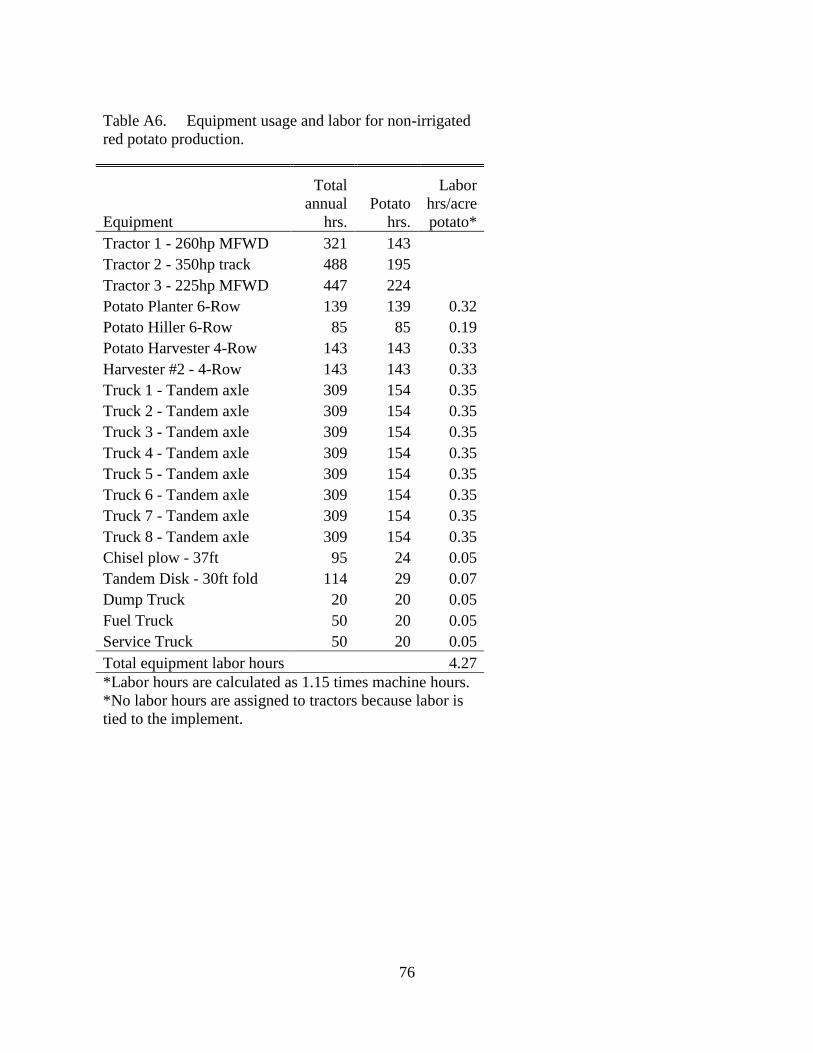
76
Table A6. Equipment usage and labor for non-irrigated
red potato production.
Equipment
Total
annual
hrs.
Potato
hrs.
Labor
hrs/acre
potato*
Tractor 1 - 260hp MFWD 321 143 Tractor 2 - 350hp track 488 195 Tractor 3 - 225hp MFWD 447 224 Potato Planter 6-Row 139 139 0.32
Potato Hiller 6-Row 85 85 0.19
Potato Harvester 4-Row 143 143 0.33
Harvester #2 - 4-Row 143 143 0.33
Truck 1 - Tandem axle 309 154 0.35
Truck 2 - Tandem axle 309 154 0.35
Truck 3 - Tandem axle 309 154 0.35
Truck 4 - Tandem axle 309 154 0.35
Truck 5 - Tandem axle 309 154 0.35
Truck 6 - Tandem axle 309 154 0.35
Truck 7 - Tandem axle 309 154 0.35
Truck 8 - Tandem axle 309 154 0.35
Chisel plow - 37ft 95 24 0.05
Tandem Disk - 30ft fold 114 29 0.07
Dump Truck 20 20 0.05
Fuel Truck 50 20 0.05
Service Truck 50 20 0.05
Total equipment labor hours 4.27
*Labor hours are calculated as 1.15 times machine hours.
*No labor hours are assigned to tractors because labor is
tied to the implement.
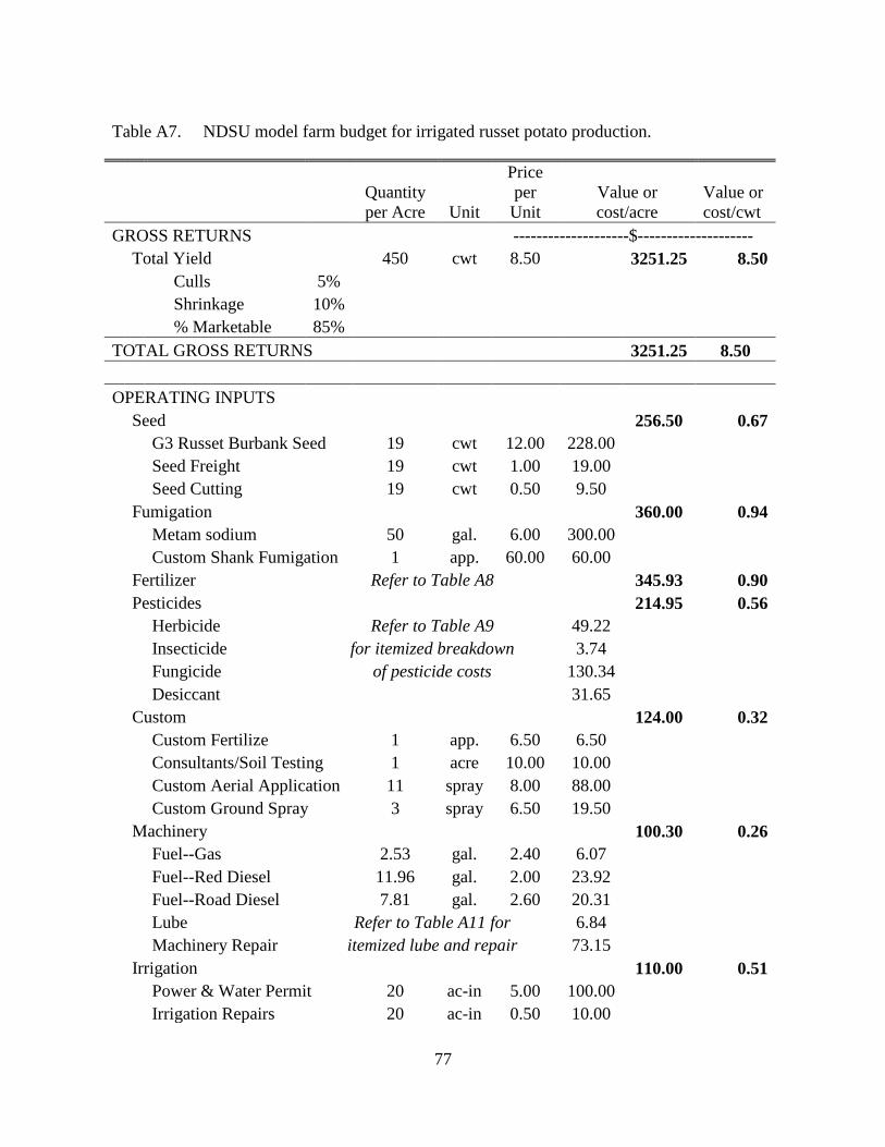
77
Table A7. NDSU model farm budget for irrigated russet potato production.
Quantity
per Acre Unit
Price
per
Unit
Value or
cost/acre
Value or
cost/cwt
GROSS RETURNS --------------------$--------------------
Total Yield 450 cwt 8.50 3251.25 8.50
Culls 5%
Shrinkage 10%
% Marketable 85%
TOTAL GROSS RETURNS 3251.25 8.50
OPERATING INPUTS
Seed 256.50 0.67
G3 Russet Burbank Seed 19 cwt 12.00 228.00
Seed Freight 19 cwt 1.00 19.00
Seed Cutting 19 cwt 0.50 9.50
Fumigation 360.00 0.94
Metam sodium 50 gal. 6.00 300.00
Custom Shank Fumigation 1 app. 60.00 60.00
Fertilizer Refer to Table A8 345.93 0.90
Pesticides 214.95 0.56
Herbicide Refer to Table A9 49.22
Insecticide for itemized breakdown 3.74
Fungicide of pesticide costs 130.34
Desiccant 31.65
Custom 124.00 0.32
Custom Fertilize 1 app. 6.50 6.50
Consultants/Soil Testing 1 acre 10.00 10.00
Custom Aerial Application 11 spray 8.00 88.00
Custom Ground Spray 3 spray 6.50 19.50
Machinery 100.30 0.26
Fuel--Gas 2.53 gal. 2.40 6.07
Fuel--Red Diesel 11.96 gal. 2.00 23.92
Fuel--Road Diesel 7.81 gal. 2.60 20.31
Lube Refer to Table A11 for 6.84
Machinery Repair itemized lube and repair 73.15
Irrigation 110.00 0.51
Power & Water Permit 20 ac-in 5.00 100.00
Irrigation Repairs 20 ac-in 0.50 10.00
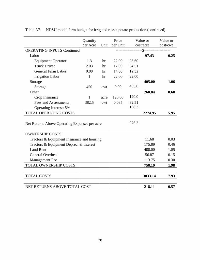
78
Table A7. NDSU model farm budget for irrigated russet potato production (continued).
Quantity
per Acre Unit
Price
per Unit
Value or
cost/acre
Value or
cost/cwt
OPERATING INPUTS Continued --------------------$--------------------
Labor 97.43 0.25
Equipment Operator 1.3 hr. 22.00 28.60
Truck Driver 2.03 hr. 17.00 34.51
General Farm Labor 0.88 hr. 14.00 12.32
Irrigation Labor 1 hr. 22.00 22.00
Storage 405.00 1.06
Storage 450 cwt 0.90 405.0
0
Other 260.84 0.68
Crop Insurance 1 acre 120.00 120.0
0
Fees and Assessments 382.5 cwt 0.085 32.51
Operating Interest: 5% 108.3
3
TOTAL OPERATING COSTS 2274.95 5.95
Net Returns Above Operating Expenses per acre 976.3
0
OWNERSHIP COSTS
Tractors & Equipment Insurance and housing 11.68 0.03
Tractors & Equipment Deprec. & Interest 175.89 0.46
Land Rent 400.00 1.05
General Overhead 56.87 0.15
Management Fee 113.75 0.30
TOTAL OWNERSHIP COSTS 758.19 1.98
TOTAL COSTS 3033.14 7.93
NET RETURNS ABOVE TOTAL COST 218.11 0.57
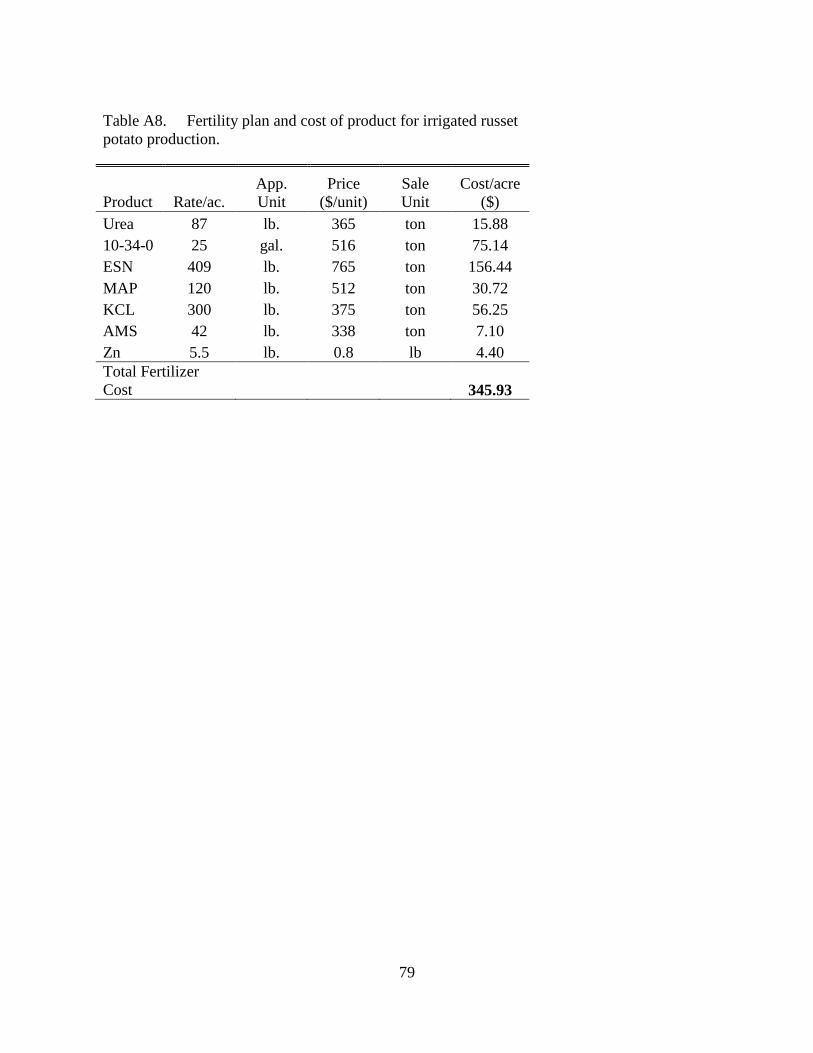
79
Table A8. Fertility plan and cost of product for irrigated russet
potato production.
Product Rate/ac.
App.
Unit
Price
($/unit)
Sale
Unit
Cost/acre
($)
Urea 87 lb. 365 ton 15.88
10-34-0 25 gal. 516 ton 75.14
ESN 409 lb. 765 ton 156.44
MAP 120 lb. 512 ton 30.72
KCL 300 lb. 375 ton 56.25
AMS 42 lb. 338 ton 7.10
Zn 5.5 lb. 0.8 lb 4.40
Total Fertilizer
Cost 345.93
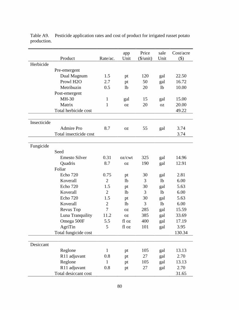
80
Table A9. Pesticide application rates and cost of product for irrigated russet potato
production.
Product Rate/ac.
app
Unit
Price
($/unit)
sale
Unit
Cost/acre
($)
Herbicide
Pre-emergent
Dual Magnum 1.5 pt 120 gal 22.50
Prowl H2O 2.7 pt 50 gal 16.72
Metribuzin 0.5 lb 20 lb 10.00
Post-emergent
MH-30 1 gal 15 gal 15.00
Matrix 1 oz 20 oz 20.00
Total herbicide cost 49.22
Insecticide
Admire Pro 8.7 oz 55 gal 3.74
Total insecticide cost 3.74
Fungicide
Seed
Emesto Silver 0.31 oz/cwt 325 gal 14.96
Quadris 8.7 oz 190 gal 12.91
Foliar
Echo 720 0.75 pt 30 gal 2.81
Koverall 2 lb 3 lb 6.00
Echo 720 1.5 pt 30 gal 5.63
Koverall 2 lb 3 lb 6.00
Echo 720 1.5 pt 30 gal 5.63
Koverall 2 lb 3 lb 6.00
Revus Top 7 oz 285 gal 15.59
Luna Tranquility 11.2 oz 385 gal 33.69
Omega 500F 5.5 fl oz 400 gal 17.19
AgriTin 5 fl oz 101 gal 3.95
Total fungicide cost 130.34
Desiccant
Reglone 1 pt 105 gal 13.13
R11 adjuvant 0.8 pt 27 gal 2.70
Reglone 1 pt 105 gal 13.13
R11 adjuvant 0.8 pt 27 gal 2.70
Total desiccant cost 31.65

81
Table A10. Whole farm equipment overhead costs for irrigated russet potatoes in dollars.
Cash Overhead Insurance & Housing Potato
overhead
per acre Equipment New cost
Years
life
Salvage
value Farm total
Potato
portion Farm total
Potato
portion
Pickup 1 - 3/4 ton 45,000 5 14,000 7,861 3,931 295 148 2.04
Pickup 2 - 3/4 ton 45,000 5 14,000 7,861 3,931 295 148 2.04
Pickup 3 - 3/4 ton 45,000 5 14,000 7,861 3,931 295 148 2.04
Pickup 4 - 3/4 ton 45,000 5 14,000 7,861 3,931 295 148 2.04
Pickup 5 - 3/4 ton 45,000 5 14,000 7,861 3,931 295 148 2.04
Pickup 6 - 3/4 ton 45,000 5 14,000 7,861 3,931 295 148 2.04
Pickup 7 - 3/4 ton 45,000 5 14,000 7,861 3,931 295 148 2.04
Pickup 8 - 3/4 ton 45,000 5 14,000 7,861 3,931 295 148 2.04
Tractor 1 - 350hp track 360,000 12 100,800 34,330 6,866 2,304 461 3.66
Tractor 2 - 350hp track 360,000 12 100,800 34,330 6,866 2,304 461 3.66
Tractor 3 - 260hp MFWD 301,000 12 84,280 28,703 22,963 1,926 1,541 12.25
Tractor 4 - 260hp MFWD 301,000 12 84,280 28,703 11,481 1,926 771 6.13
Tractor 5 - 260hp MFWD 301,000 12 84,280 28,703 11,481 1,926 771 6.13
Tractor 6 - 225hp MFWD 225,000 12 63,000 21,456 21,456 1,440 1,440 11.45
Tractor 7 - 225hp MFWD 225,000 12 63,000 21,456 21,456 1,440 1,440 11.45
Tractor 8 - 225hp MFWD 225,000 12 63,000 21,456 21,456 1,440 1,440 11.45
Potato Planter 6-Row 75,000 25 - 5,325 5,325 375 375 2.85
Planter 2 6-Row 75,000 25 - 5,325 5,325 375 375 2.85
Planter 3 6-Row 75,000 25 - 5,325 5,325 375 375 2.85
Planter 4 6-Row 75,000 25 - 5,325 5,325 375 375 2.85
Potato hiller 6-Row 25,000 30 - 1,625 1,625 125 125 0.88
Hiller 2 6-Row 25,000 30 - 1,625 1,625 125 125 0.88
Hiller 3 6-Row 25,000 30 - 1,625 1,625 125 125 0.88
Potato harvester 4-Row 160,000 20 15,000 12,350 12,350 875 875 6.61
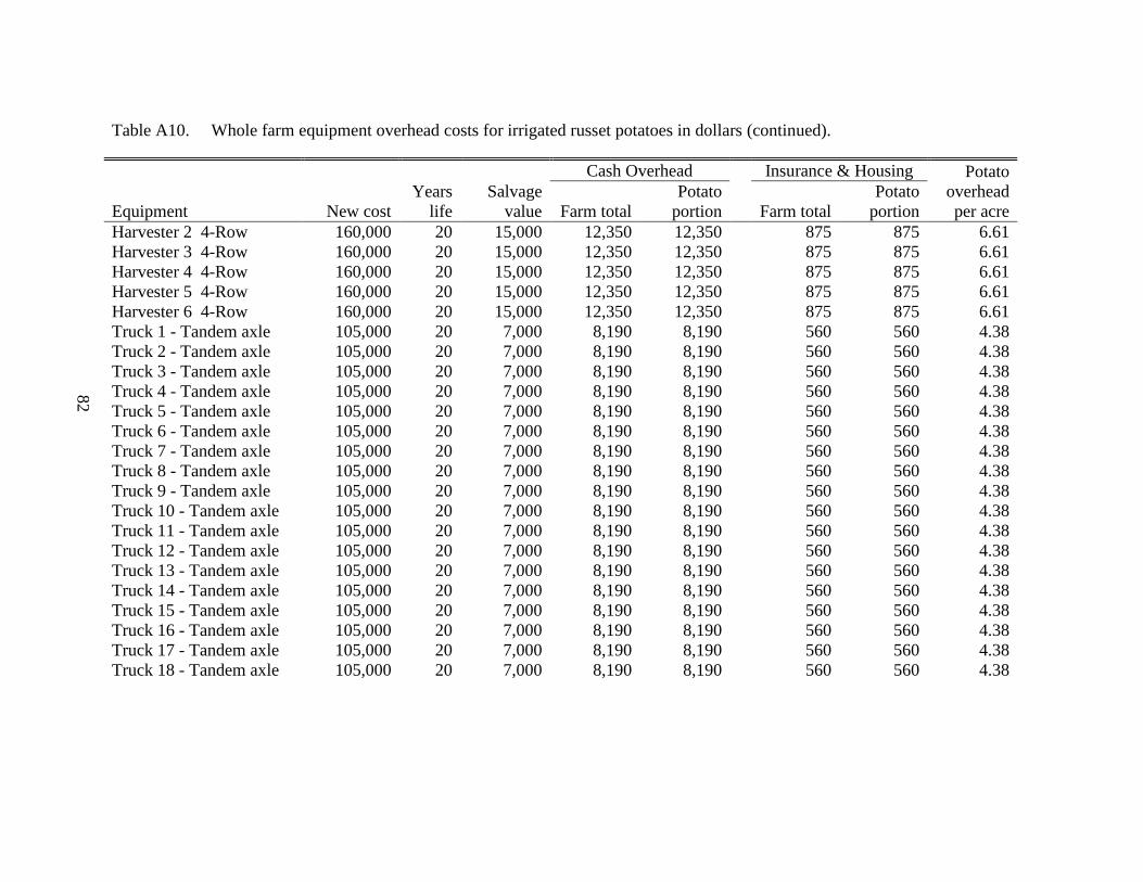
82
Table A10. Whole farm equipment overhead costs for irrigated russet potatoes in dollars (continued).
Cash Overhead Insurance & Housing Potato
overhead
per acre Equipment New cost
Years
life
Salvage
value Farm total
Potato
portion Farm total
Potato
portion
Harvester 2 4-Row 160,000 20 15,000 12,350 12,350 875 875 6.61
Harvester 3 4-Row 160,000 20 15,000 12,350 12,350 875 875 6.61
Harvester 4 4-Row 160,000 20 15,000 12,350 12,350 875 875 6.61
Harvester 5 4-Row 160,000 20 15,000 12,350 12,350 875 875 6.61
Harvester 6 4-Row 160,000 20 15,000 12,350 12,350 875 875 6.61
Truck 1 - Tandem axle 105,000 20 7,000 8,190 8,190 560 560 4.38
Truck 2 - Tandem axle 105,000 20 7,000 8,190 8,190 560 560 4.38
Truck 3 - Tandem axle 105,000 20 7,000 8,190 8,190 560 560 4.38
Truck 4 - Tandem axle 105,000 20 7,000 8,190 8,190 560 560 4.38
Truck 5 - Tandem axle 105,000 20 7,000 8,190 8,190 560 560 4.38
Truck 6 - Tandem axle 105,000 20 7,000 8,190 8,190 560 560 4.38
Truck 7 - Tandem axle 105,000 20 7,000 8,190 8,190 560 560 4.38
Truck 8 - Tandem axle 105,000 20 7,000 8,190 8,190 560 560 4.38
Truck 9 - Tandem axle 105,000 20 7,000 8,190 8,190 560 560 4.38
Truck 10 - Tandem axle 105,000 20 7,000 8,190 8,190 560 560 4.38
Truck 11 - Tandem axle 105,000 20 7,000 8,190 8,190 560 560 4.38
Truck 12 - Tandem axle 105,000 20 7,000 8,190 8,190 560 560 4.38
Truck 13 - Tandem axle 105,000 20 7,000 8,190 8,190 560 560 4.38
Truck 14 - Tandem axle 105,000 20 7,000 8,190 8,190 560 560 4.38
Truck 15 - Tandem axle 105,000 20 7,000 8,190 8,190 560 560 4.38
Truck 16 - Tandem axle 105,000 20 7,000 8,190 8,190 560 560 4.38
Truck 17 - Tandem axle 105,000 20 7,000 8,190 8,190 560 560 4.38
Truck 18 - Tandem axle 105,000 20 7,000 8,190 8,190 560 560 4.38
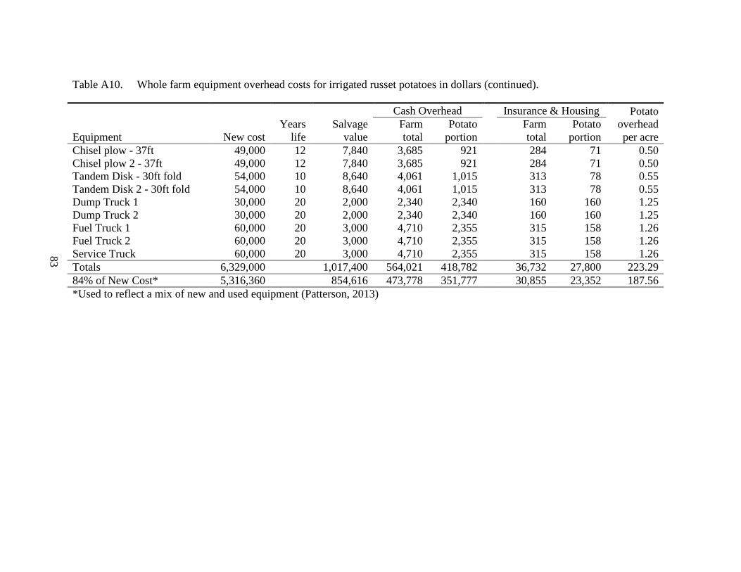
83
Table A10. Whole farm equipment overhead costs for irrigated russet potatoes in dollars (continued).
Cash Overhead Insurance & Housing Potato
overhead
per acre Equipment New cost
Years
life
Salvage
value
Farm
total
Potato
portion
Farm
total
Potato
portion
Chisel plow - 37ft 49,000 12 7,840 3,685 921 284 71 0.50
Chisel plow 2 - 37ft 49,000 12 7,840 3,685 921 284 71 0.50
Tandem Disk - 30ft fold 54,000 10 8,640 4,061 1,015 313 78 0.55
Tandem Disk 2 - 30ft fold 54,000 10 8,640 4,061 1,015 313 78 0.55
Dump Truck 1 30,000 20 2,000 2,340 2,340 160 160 1.25
Dump Truck 2 30,000 20 2,000 2,340 2,340 160 160 1.25
Fuel Truck 1 60,000 20 3,000 4,710 2,355 315 158 1.26
Fuel Truck 2 60,000 20 3,000 4,710 2,355 315 158 1.26
Service Truck 60,000 20 3,000 4,710 2,355 315 158 1.26
Totals 6,329,000 1,017,400 564,021 418,782 36,732 27,800 223.29
84% of New Cost* 5,316,360 854,616 473,778 351,777 30,855 23,352 187.56
*Used to reflect a mix of new and used equipment (Patterson, 2013)

84
Table A11. Whole farm equipment operating costs for irrigated russet potatoes in dollars.
Repairs Fuel Lube Potato
operating
cost per
acre Equipment Farm total
Potato
portion Farm total
Potato
portion
Farm
total
Potato
portion
Pickup 1 - 3/4 ton 1,620 810 3,000 1,500 450 225 1.27
Pickup 2 - 3/4 ton 1,620 810 3,000 1,500 450 225 1.27
Pickup 3 - 3/4 ton 1,620 810 3,000 1,500 450 225 1.27
Pickup 4 - 3/4 ton 1,620 810 3,000 1,500 450 225 1.27
Pickup 5 - 3/4 ton 1,620 810 3,000 1,500 450 225 1.27
Pickup 6 - 3/4 ton 1,620 810 3,000 1,500 450 225 1.27
Pickup 7 - 3/4 ton 1,620 810 3,000 1,500 450 225 1.27
Pickup 8 - 3/4 ton 1,620 810 3,000 1,500 450 225 1.27
Tractor 1 - 350hp track 3,300 660 16,133 3,227 2,420 484 2.19
Tractor 2 - 350hp track 3,300 660 16,133 3,227 2,420 484 2.19
Tractor 3 - 260hp MFWD 1,254 1,003 9,164 7,331 1,375 1,100 4.72
Tractor 4 - 260hp MFWD 1,254 502 10,400 4,160 1,560 624 2.64
Tractor 5 - 260hp MFWD 1,254 502 10,400 4,160 1,560 624 2.64
Tractor 6 - 225hp MFWD 1,500 1,500 8,582 8,582 1,287 1,287 5.68
Tractor 7 - 225hp MFWD 1,500 1,500 8,582 8,582 1,287 1,287 5.68
Tractor 8 - 225hp MFWD 1,500 1,500 8,582 8,582 1,287 1,287 5.68
Potato Planter 6-Row* 1,740 1,740 0.87
Planter 2 6-Row* 1,740 1,740 0.87
Planter 3 6-Row* 1,740 1,740 0.87
Planter 4 6-Row* 1,740 1,740 0.87
Potato hiller 6-Row* 533 533 0.27
Hiller 2 6-Row* 533 533 0.27
Hiller 3 6-Row* 533 533 0.27
Potato harvester 4-Row* 17,000 17,000 8.50

85
Table A11. Whole farm equipment operating costs for irrigated russet potatoes in dollars (continued).
Repairs Fuel Lube Potato
operating
cost per
acre Equipment Farm total
Potato
portion Farm total
Potato
portion
Farm
total
Potato
portion
Harvester 2 4-Row* 17,000 17,000 8.50
Harvester 3 4-Row* 17,000 17,000 8.50
Harvester 4 4-Row* 17,000 17,000 8.50
Harvester 5 4-Row* 17,000 17,000 8.50
Harvester 6 4-Row* 17,000 17,000 8.50
Truck 1 - Tandem axle 945 945 1,622 1,622 243 243 1.41
Truck 2 - Tandem axle 945 945 1,622 1,622 243 243 1.41
Truck 3 - Tandem axle 945 945 1,622 1,622 243 243 1.41
Truck 4 - Tandem axle 945 945 1,622 1,622 243 243 1.41
Truck 5 - Tandem axle 945 945 1,622 1,622 243 243 1.41
Truck 6 - Tandem axle 945 945 1,622 1,622 243 243 1.41
Truck 7 - Tandem axle 945 945 1,622 1,622 243 243 1.41
Truck 8 - Tandem axle 945 945 1,622 1,622 243 243 1.41
Truck 9 - Tandem axle 945 945 1,622 1,622 243 243 1.41
Truck 10 - Tandem axle 945 945 1,622 1,622 243 243 1.41
Truck 11 - Tandem axle 945 945 1,622 1,622 243 243 1.41
Truck 12 - Tandem axle 945 945 1,622 1,622 243 243 1.41
Truck 13 - Tandem axle 945 945 1,622 1,622 243 243 1.41
Truck 14 - Tandem axle 945 945 1,622 1,622 243 243 1.41
Truck 15 - Tandem axle 945 945 1,622 1,622 243 243 1.41
Truck 16 - Tandem axle 945 945 1,622 1,622 243 243 1.41
Truck 17 - Tandem axle 945 945 1,622 1,622 243 243 1.41
Truck 18 - Tandem axle 945 945 1,622 1,622 243 243 1.41
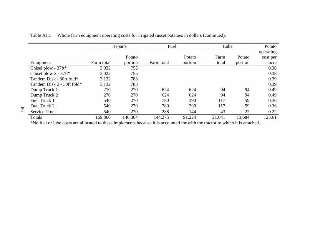
86
Table A11. Whole farm equipment operating costs for irrigated russet potatoes in dollars (continued).
Repairs Fuel Lube Potato
operating
cost per
acre Equipment Farm total
Potato
portion Farm total
Potato
portion
Farm
total
Potato
portion
Chisel plow - 37ft* 3,022 755 0.38
Chisel plow 2 - 37ft* 3,022 755 0.38
Tandem Disk - 30ft fold* 3,132 783 0.39
Tandem Disk 2 - 30ft fold* 3,132 783 0.39
Dump Truck 1 270 270 624 624 94 94 0.49
Dump Truck 2 270 270 624 624 94 94 0.49
Fuel Truck 1 540 270 780 390 117 59 0.36
Fuel Truck 2 540 270 780 390 117 59 0.36
Service Truck 540 270 288 144 43 22 0.22
Totals 169,860 146,304 144,275 91,224 21,641 13,684 125.61
*No fuel or lube costs are allocated to these implements because it is accounted for with the tractor to which it is attached.

87
Table A12. Equipment usage and labor for irrigated russet potato production.
Equipment
Total ann.
hrs.
Potato
hrs.
Labor
hrs/ac
potato Equipment (continued)
Total
ann.
hrs.
Potato
hrs.
Labor
hrs/ac
potato
Tractor 1 - 350hp track 524 105 Truck 4 - Tandem axle 196 196 0.11
Tractor 2 - 350hp track 524 105 Truck 5 - Tandem axle 196 196 0.11
Tractor 3 - 260hp
MFWD 401 320 Truck 6 - Tandem axle 196 196 0.11
Tractor 4 - 260hp
MFWD 455 182 Truck 7 - Tandem axle 196 196 0.11
Tractor 5 - 260hp
MFWD 455 182 Truck 8 - Tandem axle 196 196 0.11
Tractor 6 - 225hp
MFWD 433 433 Truck 9 - Tandem axle 196 196 0.11
Tractor 7 - 225hp
MFWD 433 433 Truck 10 - Tandem axle 196 196 0.11
Tractor 8 - 225hp
MFWD 433 433 Truck 11 - Tandem axle 196 196 0.11
Potato Planter 6-Row 139 139 0.08 Truck 12 - Tandem axle 196 196 0.11
Planter 2 6-Row 139 139 0.08 Truck 13 - Tandem axle 196 196 0.11
Planter 3 6-Row 139 139 0.08 Truck 14 - Tandem axle 196 196 0.11
Planter 4 6-Row 139 139 0.08 Truck 15 - Tandem axle 196 196 0.11
Potato hiller 6-Row 113 113 0.06 Truck 16 - Tandem axle 196 196 0.11
Hiller 2 6-Row 113 113 0.06 Truck 17 - Tandem axle 196 196 0.11
Hiller 3 6-Row 113 113 0.06 Truck 18 - Tandem axle 196 196 0.11
Potato harvester 4-Row 182 182 0.10 Chisel plow - 37ft 190 48 0.03
Harvester 2 4-Row 182 182 0.10 Chisel plow 2 - 37ft 190 48 0.03
Harvester 3 4-Row 182 182 0.10 Tandem Disk - 30ft fold 229 57 0.03
Harvester 4 4-Row 182 182 0.10 Tandem Disk 2 - 30ft
fold 229 57 0.03
Harvester 5 4-Row 182 182 0.10 Dump Truck 1 35 35 0.02
Harvester 6 4-Row 182 182 0.10 Dump Truck 2 35 35 0.02
Truck 1 - Tandem axle 196 196 0.11 Fuel Truck 1 100 50 0.03
Truck 2 - Tandem axle 196 196 0.11 Fuel Truck 2 100 50 0.03
Truck 3 - Tandem axle 196 196 0.11 Service Truck 150 75 0.04
Total equipment labor hours 3.43
*Labor hours are calculated as 1.15 times machine hours. Labor is allocated to implements not to tractors.
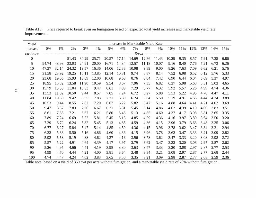
88
Table A13. Price required to break even on fumigation based on expected total yield increases and marketable yield rate
improvements.
Yield
increase
Increase in Marketable Yield Rate
0% 1% 2% 3% 4% 5% 6% 7% 8% 9% 10% 11% 12% 13% 14% 15%
cwt/acre -----------------------------------------------------------------------$/cwt------------------------------------------------------------------
0 51.43 34.29 25.71 20.57 17.14 14.69 12.86 11.43 10.29 9.35 8.57 7.91 7.35 6.86
5 94.74 48.98 33.03 24.91 20.00 16.71 14.34 12.57 11.18 10.07 9.16 8.40 7.76 7.21 6.73 6.26
10 47.37 32.14 24.32 19.57 16.36 14.06 12.33 10.98 9.89 9.00 8.26 7.63 7.09 6.62 6.21 5.76
15 31.58 23.92 19.25 16.11 13.85 12.14 10.81 9.74 8.87 8.14 7.52 6.98 6.52 6.12 5.76 5.33
20 23.68 19.05 15.93 13.69 12.00 10.68 9.63 8.76 8.04 7.42 6.90 6.44 6.04 5.69 5.37 4.97
25 18.95 15.82 13.58 11.90 10.59 9.54 8.67 7.96 7.35 6.82 6.37 5.98 5.63 5.31 5.03 4.65
30 15.79 13.53 11.84 10.53 9.47 8.61 7.89 7.29 6.77 6.32 5.92 5.57 5.26 4.99 4.74 4.36
35 13.53 11.82 10.50 9.44 8.57 7.85 7.24 6.72 6.27 5.88 5.53 5.22 4.95 4.70 4.47 4.11
40 11.84 10.50 9.42 8.55 7.83 7.21 6.69 6.24 5.84 5.50 5.19 4.91 4.66 4.44 4.24 3.89
45 10.53 9.44 8.55 7.82 7.20 6.67 6.22 5.82 5.47 5.16 4.88 4.64 4.41 4.21 4.02 3.69
50 9.47 8.57 7.83 7.20 6.67 6.21 5.81 5.45 5.14 4.86 4.62 4.39 4.19 4.00 3.83 3.51
55 8.61 7.85 7.21 6.67 6.21 5.80 5.45 5.13 4.85 4.60 4.37 4.17 3.98 3.81 3.65 3.35
60 7.89 7.24 6.69 6.22 5.81 5.45 5.13 4.85 4.59 4.36 4.16 3.97 3.80 3.64 3.50 3.20
65 7.29 6.72 6.24 5.82 5.45 5.13 4.85 4.59 4.36 4.15 3.96 3.79 3.63 3.48 3.35 3.06
70 6.77 6.27 5.84 5.47 5.14 4.85 4.59 4.36 4.15 3.96 3.78 3.62 3.47 3.34 3.21 2.94
75 6.32 5.88 5.50 5.16 4.86 4.60 4.36 4.15 3.96 3.78 3.62 3.47 3.33 3.21 3.09 2.82
80 5.92 5.53 5.19 4.88 4.62 4.37 4.16 3.96 3.78 3.62 3.47 3.33 3.20 3.08 2.98 2.72
85 5.57 5.22 4.91 4.64 4.39 4.17 3.97 3.79 3.62 3.47 3.33 3.20 3.08 2.97 2.87 2.62
90 5.26 4.95 4.66 4.41 4.19 3.98 3.80 3.63 3.47 3.33 3.20 3.08 2.97 2.87 2.77 2.53
95 4.99 4.70 4.44 4.21 4.00 3.81 3.64 3.48 3.34 3.21 3.08 2.97 2.87 2.77 2.68 2.44
100 4.74 4.47 4.24 4.02 3.83 3.65 3.50 3.35 3.21 3.09 2.98 2.87 2.77 2.68 2.59 2.36
Table note: based on a yield of 350 cwt per acre without fumigation, and a marketable yield rate of 76% without fumigation.