Steady-State and Transient Boundary Element Methods for ... · Steady-State and Transient Boundary...
58
NASA Technical Memorandum 110427 Steady-State and Transient Boundary Element Methods for Coupled Heat Conduction Dean A. Kontinos, Thermosciences Institute, Ames Research Center, Moffett Field, California Janua@ 1997 National Aeronautics and Space Administration Ames Research Center Moffett Field, California 94035-1000 https://ntrs.nasa.gov/search.jsp?R=19970011271 2018-08-27T03:47:49+00:00Z
Transcript of Steady-State and Transient Boundary Element Methods for ... · Steady-State and Transient Boundary...

NASA Technical Memorandum 110427
Steady-State and TransientBoundary Element Methods forCoupled Heat Conduction
Dean A. Kontinos, Thermosciences Institute, Ames Research Center, Moffett Field, California
Janua@ 1997
National Aeronautics andSpace Administration
Ames Research CenterMoffett Field, California 94035-1000
https://ntrs.nasa.gov/search.jsp?R=19970011271 2018-08-27T03:47:49+00:00Z


Contents
Page
Nomenclature ................................................................................................................................ v
Summary ....................................................................................................................................... 1
1 Introduction .......................................................................................................................... 1
2 Governing Equations ............................................................................................................ 3
3 Steady-State Boundary Element Algorithm ......................................................................... 5
3.1 The Boundary Integral Equation .............................................................................. 5
3.2 Fundamental Solution for Two-Dimensional, Steady-State Heat Conduction ........ 9
3.3 Element Shape Function .......................................................................................... 10
3.3.1 Orientation 1 Distance Function ............................................................... 10
3.3.2 Orientation 2 Distance Function ............................................................... 12
3.3.3 Orientation 3 Distance Function ............................................................... 12
3.4 Solution Variable Interpolation Function ................................................................ 13
3.5 Integral Transforms .................................................................................................. 14
3.5.1 Orientation 1 Integrals .............................................................................. 14
3.5.2 Orientation 2 Integrals .............................................................................. 15
3.5.3 Orientation 3 Integrals .............................................................................. 15
3.6 Numerical Results .................................................................................................... 16
3.6.1 Cylinder ..................................................................................................... 16
3.6.2 Pin Cushion ............................................................................................... 17
3.6.3 Nonconvex Polygon .................................................................................. 19
Transient Boundary Element Algorithm .............................................................................. 21
4.1 The Boundary Integral Equation .............................................................................. 21
4.2 Fundamental Solution for Two-Dimensional, Transient Heat Conduction ............. 24
4.3 Time-Step Procedure ................................................................................................ 25
4.4 Element Shape Functions and Integral Transforms ................................................. 27
4.4.1 Nonsingular Integrals ................................................................................ 28
4.4.2 Singular Integrals ...................................................................................... 34
4.5 Numerical Results .................................................................................................... 42
4.5.1 One-Dimensional Rod ............................................................................... 42
4.5.2 Two-Dimensional Plate ............................................................................. 43
4.5.3 One-Dimensional Rod with Fluctuating Boundary Condition ................. 45
5 Conclusion ........................................................................................................................... 48
References ..................................................................................................................................... 49
4
°.,
111


Steady-State and Transient Boundary Element Methods
for Coupled Heat Conduction
Dean A. Kontinos
Ames Research Center
Summary
Boundary element algorithms for the solution of steady-state and transient heat conduction are
presented. The algorithms are designed for efficient coupling with computational fluid dynamic
discretizations and feature piecewise linear elements with offset nodal points. The steady-state
algorithm employs the fundamental solution approach; the integration kernels are computed analyti-
cally based on linear shape functions, linear elements, and variably offset nodal points. The analytic
expressions for both singular and nonsingular integrands are presented. The transient algorithm
employs the transient fundamental solution; the temporal integration is performed analytically and
the nonsingular spatial integration is performed numerically using Gaussian quadrature. A series
solution to the integration is derived for the instance of a singular integrand. The boundary-only
character of the algorithm is maintained by integrating the influence coefficients from initial time.
Numerical results are compared to analytical solutions to verify the current boundary element
algorithms. The steady-state and transient algorithms are numerically shown to be second-order
accurate in space and time, respectively.
1 Introduction
Computational science is advancing dramatically in these first decades of the Information Age.
Performance gains in computer technology are propelling scientific computing to the forefront of the
engineering process. Increasing processor speed is promoting greater fidelity of the physical models,
and increases in memory are permitting finer resolution of the physical domain. Simulations, once
impossible to perform in a timely fashion, are routinely computed using desktop workstations.
Furthermore, computational mQdeling is extending into every theatre of engineering, for example,
fluid dynamics, acoustics, heat transfer, chemistry, astrophysics, and structural mechanics.
Although the maturing numerical methodology is applicable across the engineering spectrum,
much of the development is compartmentalized into the separate disciplines. For example, in the
aerospace industry, computational fluid dynamics (CFD) simulations performed in the aerodynamics
or propulsion group are passed, sometimes blindly, as a load condition to the structures group
wherein a structural dynamic simulation is computed. To bridge this gap, the latest effort in compu-
tational science is coupling analysis codes across disciplines. This effort is a natural path of develop-
ment, but, more importantly, it is being driven by engineering systems whose complexity dictates a
coupled analysis. For instance, in the silicon chip fabrication industry, accurate simulation of

chemicalvapordepositionandchemicaletchingrequiresmodelingof thefluid dynamicsin thereactorcoupledto asurfacechemistrymodel.In theaerospacefield, advancedhypersonicconceptsblendthepropulsionsystemwith thebodymoldline, therebyblurring thetraditionalindustrydemarcationsof aerodynamics,propulsion,andstructure.Also,metallic thermalprotectionpanelsarebeing implementedfor thenewreusablelaunchvehicle.Becauseof aerodynamicheating,thepanelsexpandfrom thestructureandalterthehypersonicflow field.Analysisof thethermalprotec-tion systemrequirescouplingof theaerothermodynamicsto thestructuralresponse.It is in this arenaof coupledCFDto structuralanalysisthatthediscussionis focused.
Two basicapproachesareusedto solvecoupledfluid/structuralsystems.Thefirst is a directcouplingwherethesolutionof thedifferent fieldsis solvedsimultaneouslyin onelargesystemofequations.Direct coupling is mostlyapplicablefor problemswheretime accuracyis critical, suchasin aeroelasticitywherethetimescaleof thefluid motionis onthesameorderasthestructuralmodalfrequency.Thesecondapproachis a loosecouplingstrategywhereeachsetof field equationsissolvedto produceboundaryconditionsfor theother.Theequationsaresolvedin turnuntil aniteratedconvergencecriterion is metatthefluid/solidinterface.It is notwithin thescopeof thispaper,nor in theexpertiseof theauthor,to presentacomprehensiveliteraryreview of coupledCFD-structuraldynamicmethods.Instead,reference1is recommended,whereinabrief bibliographyandacoupledsimulationis given.
Theloosecouplingstrategyis particularlyattractivewhencouplingsolidmechanicstohypersonicCFD.Thetime scalesof thehypersonicflow field areoftendisparatefrom thetimescalesof thestructure,therebyobviatingadirectlycoupledtime-accurateanalysis.Furthermore,high-speedflows arerepletewith complexphysicalphenomenasuchasshockwaves,shock-wave/boundary-layerinteractions,chemicalreactions,andinternalenergyexchange.Thenumericsforhypersonicalgorithmsaresophisticatedand,attimes,temperamental.Adding structuralequationsto thesystemmaydiminish therobustnessof thecraftedhypersonicCFDcode.Thus,the loosecoupling strategyeffectivelyshieldstheCFDcodefrom performancedegradationwhile increasingthefidelity of theglobalsimulation.
In theaerospaceindustry,finite elementandfinite differencemethodsareroutinelyusedfor thesolutionof solid heatconductionandelasticity.Well proven,thesemethodsarereadilyavailableforloosecouplingwith aCFDcode.A thirdoption,rarelyusedin theaerospacecommunity,is theboundaryelementmethod(BEM).Li andKassab(refs.2 and3) haveefficiently solvedjoint fluidandstructuralheatingby couplingCFDto theBEM solutionof theconductionin thebody.Theadvantageof theBEM overafinite differenceor finiteelementformulationis that only theboundaryis discretized,andthusthedimensionalityof theproblemis reduced.As aresult,it is naturallycoupledwith CFD. Theboundaryelementgrid is simplytheCFDgrid atthefluid/surfaceinterfaceplus additionalgrid pointsdefiningtheboundariesof thebody.Theinteriorof thedomainis notdiscretized.This reductionin dimensionalityisespeciallyadvantageouswhencouplingto CFDbecauseinterior valuesaresuperfluous;only surfacevaluesarerequiredfor coupling.Consequently,theBEM is potentiallymoreefficientthanfinite differenceor finite elementmethodswhichrequireaninterior discretizationto producesurfaceconditions.UsingtheBEM, thetemperaturecanbecomputedat anydesiredinteriorpoint throughcontourintegralsover theboundarysolution. Insummary,advantagesof theBEM area reductionof dimensionality,easeof discretization,andefficient couplingwith CFD.
2

Acronyms
BEM
CFT)
Symbols
A,B,C,Q
A1, A2
a,b
CpC
Cl, c2
Dj
e
et
F
Gjk, Hjk
H
Ijsl_ r
k,
le
n, fi, nj
Qj
qj
C_
F
7
Nomenclature
boundary element method
computational fluid dynamics
distance function coefficients
integration coefficients
nodal offset values
domain view factor at source point
heat capacity coefficient
coefficients
vector matrix containing domain integration coefficients
internal energy per unit volume
total energy per unit volume
arbitrary function
matrices containing influence coefficients
Heaviside function
steady-state component integrals
transient component integrals
tensor thermal conductivity
scalar thermal conductivity
length of linear element
outward unit normal
position vector to the point source
vector matrix containing nodal temperature gradients
temperature gradient boundary condition
heat flux in index notation
position vector to arbitrary point in the domain
distance from source point to point in domain
vector from source point to point in domain

S
T
T
"6
T"
xjTo
t
tf
to
U
uj, u k
V
W
W,W
W $S
W tr
x,y
xj
F
6
E
7?
,;l., O,
P
T
surface
temperature
temperature boundary condition
numerical approximation of the temperature
numerical approximation of the temperature defined by equations (3.1 la) or (4. lOa)
initial temperature
perturbation temperature
vector matrix containing nodal temperature
reference temperature
time
final time
initial time
dummy integration variable
velocity in index notation
volume
domain weight function
boundary weight functions
fundamental solution for steady-state conduction
fundamental solution for transient conduction
spatial coordinates
spatial coordinates in index notation
thermal diffusivity
domain boundary
integration limit
Dirac delta function
error residual
transformed temporal coordinate
polar transform variables
transformed spatial coordinate
solid density
time
vi

¢I_j k
Zi
O9
Subscripts
e
i,j,k,m
P
q
F
f_
Superscripts
ss
tr
viscous dissipation in index notation
solution variable interpolation function
local transformed temporal coordinate
domain
parameter, defined by equation (3.33)
denotes element
indices
denotes source point
denotes node point
denotes boundary
denotes domain
denotes steady-state
denotes transient
vii


This paper presents BEM algorithms for two-dimensional, steady-state and transient, heat
conduction. The algorithms are specifically designed for efficient coupling with CFD. The presen-tation includes a brief tutorial on the BEM for those unfamiliar with the technique. Then the details
of the current algorithms are presented. The mathematics are overly detailed because the paper is
intended as a technical reference manual to document the algorithms. The document is organized as
follows: The governing equation of heat conduction is given in Chapter 2, the steady-state algorithm
with numerical examples in Chapter 3, and the transient algorithm with numerical examples in
Chapter 4.
2 Governing Equations
Consider a material volume in space with no internal heat generation. Applying the conservation
of energy, the time rate of change of the volumetric internal energy is equal to the net flux of energy
through the bounding surface; in index notation, this relation is
3-_ Iet dV+ I(etuj+_jkUk+qj)njdS=O
Volume Surface
(2.1)
where et is the total energy per unit volume, uj is the velocity of the particles, dPjk is the viscous
dissipation, qj is the heat flux, nj is the outward unit normal, and t is time. In a solid, the materialvelocity is zero; therefore, the convection and viscous dissipation terms are zero. Furthermore,
since the kinetic energy is zero, the total energy comprises only the internal mode. Applying the
Divergence Theorem, equation (2.1) becomes
-_ e dV + _ dV=OVolume Volume
(2.2)
where e is the internal energy and xj are the independent spatial variables. Expressions for the
internal energy and the heat flux are now established. The internal energy of a solid is empirically
determined through the heat capacity, denoted as c, defined as the change in heat content of the solid
per change in degree of temperature. In general, c is determined experimentally over a range of
temperatures. The relation is
1 dec - (2.3)
p dT
The internal energy is found by integrating cdT from a given reference temperature, T0, to the
temperature of interest,
T
e = p I c dT (2.4)
ro
3

If c is independent of temperature, then the internal energy simplifies to
e=pcT (2.5)
In general, the heat flux comprises radiative and conductive terms. Neglecting radiation, the heat
flux is given by Fourier's law, which states that the conductive flux is proportional to the tempera-
ture gradient. In index notation, Fourier's law is
qk = -Kjk "_j (2.6)
where Kjk is the thermal conductivity. In general, the thermal conductivity is a tensor quantity thatis a function of position, direction, and temperature. For this analysis, however, the thermal conduc-
tivity is considered to be a scalar quantity denoted as ks. Thus, modifying equation (2.6) for scalar
conductivity and substituting equations (2.5) and (2.6), the energy conservation law (eq. (2.2)),
becomes
0T _9dV = 0 (2.7)
In equation (2.7), the time derivative is pulled inside the volume integral; this operation is valid as
long as the limits of integration are time independent, i.e., the domain is fixed. Letting the volume
shrink to zero, the differential form of the heat conduction equation is derived as
0Tm-g =v.(ksV:r) (2.8)
For a constant thermal conductivity equation (2.8) reduces to
o_ = aV2T (2.9)&
where c_ = ks/(Pc) is the thermal diffusivity. At the steady state, the time derivative of temperature
is zero and the heat conduction equation reduces to Laplace's equation, given as
V2T = 0 (2.10)
In summary, the transient heat conduction equation given by equation (2.8) is valid for a solid
material with a constant c. Further simplification of a constant scalar conductivity yields equa-
tion (2.9), which is the transient conduction equation expressed in terms of the thermal diffusivity.
Finally, in the steady state, equation (2.9) reduces to Laplace's equation, given by equation (2.10).
4

3 Steady-State Boundary Element Algorithm
This section develops the boundary element procedure for solving steady-state heat conduction.
For completeness, a derivation of the boundary integral equation is presented. The presentation is
self-contained, yet is only cursory in detail. Definitive presentations on the BEM are found in
references 4 through 6. Regardless of the potential insufficiencies, the derivation of the boundary
integral equation is presented through weighted residual analysis. Next, the weight function, which
appears in the boundary integral equation as the kernel of an integral transform, is chosen to be
Green's free space solution to the governing equation. The free space solution and its directional
derivative are specified in this section. Then, shape functions are presented for a linear distribution
of the dependent variables over linear boundary elements with offset nodes. Analytic expressions for
the integral transforms are given for both singular and nonsingular integrands. Finally, test cases are
presented.
3.1 The Boundary Integral Equation
The core of the boundary element method is the boundary integral equation. Equation (2.10) is
the starting point for the derivation of the boundary integral equation for steady-state heat conduc-
tion. The derivation is presented through the perspective of a weighted residual analysis based upon
presentations in references 4 and 6. Let f2 be the solid domain with boundary F upon which
equation (2.10) is valid. Furthermore, let the boundary be divided into two parts, F 1 and F 2, for
which the following boundary conditions apply:
T= Ton F 1 (3.1a)
_- = g on F2 (3.1b)
Further subdivision of the boundary does not enhance the validity of the derivation; it only adds to
the complexity of the algebra.
The goal of any numerical approximation is to minimize the error in the satisfaction of the
governing equation and the boundary conditions. Frequently, the numerical scheme is designed to
satisfy the boundary conditions exactly, and the error is minimized on the interior. For this deriva-
tion, however, the strict enforcement of the boundary condition is relaxed; the numerical scheme is
constructed to minimize the error over the domain and the boundary. Let i? represent the numerical
approximation to T, and let e be the error residual. Over the domain and boundary, the error is
given by
_ = V2T (3.2a)
eF_ = 7_ - V (3.2b)
5

- _ (3.2c)er2 = &
In weighted residual analysis, the error residuals are multiplied by weight functions and integrated
over the domain and boundary to measure the global error. The weight functions can be viewed as
error distribution functions whose choice determines the type of numerical approximation. For
example, the method of Galerkin is obtained by choosing the weight functions from the same classof functions used to describe 7_. An instructive presentation of the weighted residual approach and
its connection to finite difference, finite element, and least-squares techniques is given in refer-
ence 6. The weighted residual expression based on the error residuals of equations (3.2) is given as
j" ef2W d_ + [ eFl W" dl" + _ £:F2W dl-" = 0
rl rE
(3.3)
m
where W is the weight function over the domain and W and W are the weight functions over the
boundary. Substituting in the residual expressions of equations (3.2) yields
F1
(3.4)
The boundary integral equation is derived by manipulating the domain integral and judiciously
choosing the weight functions. From the weighted residual perspective, the steps of the derivation
appear prescient in their introduction; indeed, the source of the foreknowledge is the original
formulation from reciprocity considerations. Rizzo (ref. 7) presents an interesting and informative
historical view of the boundary integral technique wherein the derivation is far more deductive
than that presented herein. Nevertheless, the focus is on transforming the domain integral of equa-
tion (3.4) into a more convenient form. This transformation is accomplished by applying Green's
identity to the domain integral to reduce the order of the operator on the temperature field. The
relation is given by
j w vw.vfd.+ j"wv¢. erf2 f2 F
(3.5)
Substitution of equation (3.5) for the domain integral of equation (3.4) produces the weak form
of the residual statement, which is the basis of the finite element method. In the weak form, the
weight function is symmetric to the numerical solution and, depending on the choice of the weight
function, frequently gives rise to symmetric matrices. To produce the boundary integral equation,
Green's identity is applied a second time to transfer the Laplacian operator to the weight function.
Transposing the role of T and W, equation (3.5) is rearranged to yield
j vw. v: d. = j v w,t. +j ¢vw., _ F
(3.6)

Successive substitution of equations (3.6) and (3.5) into equation (3.4) yields
F2
(3.7)
By consecutive application of Green's identity, the Laplacian operator in the domain integral hasbeen transferred from the numerical solution to the weight function. This formulation is termed the
inverse problem, and upon its derivation, attention is turned to the weight functions.
Up to this point, the only limiting assumption is that the weight function, W, must be twice
differentiable in order to apply Green's theorem consecutively. There is complete freedom in
selecting the boundary weights; they are chosen such that
-- 0wW = --_-on F1 (3.8a)
W = -W on F 2 (3.8b)
Substituting equations (3.8) into equation (3.7) and noting the cancellations in the boundary integrals
results in
£-2 F 2 F1 F1 F2
(3.9)
By consolidating the notation, the boundary integrals can be simplified to yield
%- arC+f_ F F
(3.10)
where
If? over f2 and on F2f=LTon rl
gonF2
It is instructive to review the steps leading to equation (3.10). First, a weighted residual statement
is written with separate weight functions for the boundaries and the domain. Green's theorem is
applied to yield the inverse problem shown in equation (3.7). Then the boundary weight functions
(3.1 la)
(3.1 lb)

are selected in terms of the interior weight function to produce cancellation in the boundary
integrals. Finally, a judicious variable change simplifies the integral equation.
The remaining task is the selection of the weight function; a profitable choice is Green's free
space solution to the governing equation. Green's function is a fundamental solution to the govern-
ing equation subject to a unit impulse forcing function. The fundamental solution for steady-state
conduction, denoted by W ss, satisfies
V2wss = a(_l - _) (3.12)
where S is the Dirac delta function, ,?/is a position vector to any point in the domain, and _ is the
position vector to the point source. The precise mathematical definition of the Dirac function is
ambiguous, but its critical property is that, for a function F(x), the integral of the product of
F(x)_(x - x O) satisfies
_F(x) O(x-xo)df_=F(x O)(3.13)
In some presentations, the Dirac function is defined by equation (3.13), and in some instances,
equation (3.13) is a property of the definition; a more extensive discussion of the Dirac function is
given in reference 8. In any case, the operation of the Dirac function in lieu of V2W ss in the domain
integral isolates the value of the temperature at the source point. The domain integral is effectively
eliminated. The boundary integral equation becomes
F F
(3.14)
where Tp is the numerical approximation of the temperature at the source point p. The coefficient
Cp is a function of the included angle exposed to the interior at the source point. Details of the
derivation of Cp are given in reference 4.
The boundary integral equation is the core of the boundary element method. By choosing the
fundamental solution as the weight function, domain integration has been eliminated; observe from
equation (3.14) that only boundary integrals appear. The result of this development is a numerical
procedure where the nodal points are located only on the boundary. The boundary-only characterstands in contrast to finite difference or finite element techniques that require a complete domain
discretization; the benefit is a reduction in dimensionality. Furthermore, with the BEM any subset
of the interior solution can be calculated to any desired resolution based on the computed boundary
solution.
The general outline of the BEM is as follows: The boundary is discretized into elements that can
be of any shape, but typically are polynomials as in finite element procedures. The solution variables
are assigned an interpolation function based on nodal points distributed over the element. The inter-
polation function defines the distribution of the solution variable over the element. Originating at the

sourcepoint, thefundamentalsolutionandits directionalderivativearekernelsof anintegraltransformof theprescribedinterpolationfunctions.After dividing theboundaryinto elements,theboundaryintegralequationbecomes
3WSS __-2 f + WSS --0eF e eF e
(3.15)
where e denotes an individual element, so Te and o'_e/On denote the distribution of the dependent
variables over element e. Typically, the integrals are computed numerically using Gaussian
quadrature.
Equation (3.15) is written for each node to form a system of linear equations. The system is
expressed in matrix notation as
HjkTj + GjkQj = 0(3.16)
where Tj and Qj are vectors containing the nodal temperatures and temperature gradients,
respectively, and l-Ijk and Gjk are matrices containing the influence coefficients resulting fromthe integral transform. After segregating the known and unknown dependent variables based on the
boundary conditions, the linear system is solved to yield the complete solution on the boundary.
The algorithms presented in this paper employ Gaussian elimination with partial pivoting for direct
inversion of the system matrix. To compute the interior solution, equation (3.15) is applied with the
source point located at the interior point of interest. Since the solution on the boundary is completely
known, the boundary integrals are computed directly without a matrix inversion.
The remaining ingredients of the numerical recipe are the definition of the fundamental solution
and its derivative, the geometrical definition of the boundary element, and the prescription of the
approximating interpolation function to the unknown solution variables T and O7"/On. The combi-
nation of these ingredients differentiates particular boundary element algorithms. The algorithms
presented here are specifically designed for efficient coupling with a CFD flow solver. Serendipi-
tously, an analytic solution of the integral transforms is achieved with the chosen combination of
ingredients.
3.2 Fundamental Solution for Two-Dimensional, Steady-State Heat Conduction
The fundamental solution for the two-dimensional Laplace's equation is given by
wSs=_l in1 (3.17)2zr r
where r is the distance from the source point to a point in the domain; it is expressed as
r = I1 11= - (3.1 S)

Thedirectionalderivativeis givenas
tgW ss 1 ?eh
oan 2 _r r 2(3.19)
Both the fundamental solution and its derivative are singular at r = 0, so care must be taken when
integrating near or through the source point.
3.3 Element Shape Function
The next ingredient to the numerical recipe is the definition of the boundary element shape. The
element shape is distinct from and prescribed independently of the dependent variable distribution.
The element shape is a geometrical attribute that determines the distance function, the outward
normal, and the integration path of the contour integrals. On the other hand, the dependent variable
interpolation function defines the distribution of the dependent variables over the element. The two
functions are constrained differently; the element shape is determined by the physical domain,
whereas the interpolation function is governed by the variation of the solution over the boundary.
The two functions combine to determine the accuracy of the algorithm. The element shape function
is given in this section while the variable interpolation function is described in the next.
This boundary element algorithm is specifically designed for coupling with CFD codes that
employ finite difference or finite volume techniques. For both structured and unstructured grids,
these CFD techniques assume linear segments between grid points. Thus, linear boundary elements
are selected in order to ensure one-to-one correspondence of the boundary element grid to the CFD
grid. With linear elements, conservation is easily satisfied since interpolation is not required to mate
the two domains. Furthermore, employing linear boundary elements creates two simplifications.
First, the distance function, r, is prescribed analytically between any arbitrary point and line seg-
ment. Second, the outward unit normal to a linear element remains constant; consequently, _ • r/,
which arises from the directional derivative of the fundamental solution, is pulled out of the
integration. These simplifications allow analytic solution of the integral transforms.
The component expressions for r and ? • h for a linear element are now presented. In two-
dimensional space, the source point can be oriented with respect to a linear segment in one of three
possible ways. Each orientation results in a different analytic expression and is addressed separately.
In Orientation 1, the source point is not collinear with the line segment; thus, _ • h _: 0. For Orien-
tation 2, the source point and element are collinear but the source point does not lie on the segment
itself. Finally, in Orientation 3, the source point lies on the element; thus, the element contains an
integrable singularity. In both Orientations 2 and 3, _ • h = O.
3.3.1 Orientation 1 Distance Function- Figure 1 displays the notation and schematic of a source
point and linear boundary element in Orientation 1; ? is the position vector from the source point to
a point on the element; F12 is the position vector from the first point of the line segment to the end
point; and rpl is the position vector from the source point to the first point of the line segment. Theelement is mapped into a linear segment of unit length through the transformation
10

(x2, Y2)
J, Yl)
Fpl \ \
(xp, yp)
Figure 1. Source point and linear boundary element segment in Orientation 1.
X = x 1 +_(X 2 -X 1)
Y = Yl + _(Y2 - Yl)
where (x 1,Yl ) and (x 2, Y2 ) are the start and end coordinates, respectively, of the line segment
defining the element, and _ is the transform variable with range 0 < _ < 1. The square of the
distance function varies as a quadratic function of the transform variable according to
r 2 =ror =A+B_+C_ 2
(3.20a)
(3.20b)
(3.21)
where
A= rpl " Fpl
B = 2Fpl • r12
C = _12 " r12
(3.22a)
(3.22b)
(3.22c)
The coefficients A, B, and C are solely functions of the geometry; they attain different values for
each element and source point combination.
11

The magnitude of the dot product of the position vector and the element outward unit normal can
be expressed in terms of the distance function coefficients as
17• hi = _ (3.23)
where
Q = 4AC- B 2 (3.24)
By ordering the elements in a counterclockwise fashion by convention, the sign of the dot product is
determined by
sign(? • h) = sign(_pl x _12) (3.25)
Note that the dot product becomes zero when Q is zero.
3.3.2 Orientation 2 Distance Function- In Orientation 2, the source point is collinear with the
element. As will be shown later, the analytic expressions of the integration become undefined when
the source point and line segment are collinear, i.e., when Q = 0. This degeneracy is avoided by
redefining the distance function. Since the source point and element are collinear, the location of the
source point can be expressed in terms of the element transform variable _. Let _p be the position
of the source point. Recall that the element is defined over the range 0 < _ < 1 ; thus, if 0 < _p < 1,
then the source point lies on the line segment resulting in Orientation 3. In Orientation 2, the source
lies off the element, so _p > 1 or _p < 0. In either case, _p is determined as
-B
_p = -_ (3.26)
The distance function becomes
_/-__ _r_ for _p > 1
r = _/-_ + ¢_/-_ for _p < 0(3.27)
3.3.3 Orientation 3 Distance Function- In the third orientation, the source point lies on the
element and hence the integral transform is singular at a point along the path of integration. Never-
theless, the integral transform exists in the Cauchy principle value sense. In order to compute the
principle value, it is convenient to set the origin of the transform variable at the source point. Such
a transformation is dependent on the location of the source point with respect to the grid points;
consequently, it is dependent on the solution variable shape function. Therefore, the discussion of
the distance function for Orientation 3 is delayed until after the presentation of the solution variable
interpolation function in the next section.
12

3.4 Solution Variable Interpolation Function
The final ingredient of the numerical recipe is the dependent variable interPOlation function.
Barring an algorithm designed for a specific application, it is common to set the interpolationfunction to the same order as the element shape because, in general, the least accurate function will
constrain the global accuracy. Thus, the distribution of the solution variables is selected to be linear.
Two node points are required on each element to properly define a linear distribution. Normally in
finite difference and finite element methods the node points are coincident with the grid points or,
in other words, the node points are located at the ends of the linear element. For piecewise linear
segments, however, the element normal direction will most likely change discontinuously from one
element to the next. Consequently, when the nodal points are coincident with the grid points, the
node normal direction, which is used to define cgT/On, becomes nonunique at the node. There are
procedures to account for this effect, which amount to substituting an auxiliary equation when
relating the upstream and downstream temperature gradients of a particular grid-node point (for
example, see ref. 9). In the present work, the node points are variably offset from the ends of the line
segment. The placement of the node away from the grid point uniquely defines the element normalat the node. The drawback of the offsetting strategy is an increase in the number of nodes since, in
general, two unique nodes per element are required, whereas a node located at the grid point is
common to the two adjoining elements. This offsetting procedure is not required in all circum-
stances. For instance, if two adjoining elements are collinear, then the node point is placed at the
grid point without concern. Since minimizing the number of nodes to reduce the computational
effort is desirable, a shape function that accounts for variable positioning of the node is described.
Figure 2 shows an element and the position of the nodal points. The nodes are offset from the
beginning and end grid points by transformed distances a and b, respectively. If the value of a or b
is zero, then the grid and node point are coincident. Let _e represent either of the solution variables
or c)7"/_?n over element e. Also, let _e,1 and _e,2 be the values of the solution variable at the
beginning and end nodes of element e, respectively. The solution variable is given by the linear
function
1 [_e,l(l_b__)+_e,2(__a) ]_e = (1-b-a)(3.28)
Although not indicated by a subscript e, the values of a and b vary from element to element,
depending on the local geometry and boundary conditions.
• Grid Point
o Node Point
_e.1 _e,2 (xz,y2)(xl,yl)v v
I I I I
=0 _=a _ =l-b _=1
Figure 2. Linear boundary element definition.
13

3.5 Integral Transforms
Definitions of the weight function, the element shape, and the variable distribution function are
now complete. These elements are combined to derive analytic expressions for the integral trans-
forms. Two integrals are computed for each element and source point combination. The integrals
are mapped into the transform variable _ and are given as
0W ss t.l_ 9W ss
7"e----_dF = le JoTe _
re
(3.29a)
fwss_dF l [1wSS-_-d_= ej0
re
(3.29b)
where le is the length of the element. Recall that the distance function and dot product contained inthe fundamental solution and the solution variables have all been previously expressed in terms of
_. The integral expressions are analytically derived for each of the three possible orientations.
3.5.1 Orientation 1 Integrals- In this orientation, the fundamental solution, with the expression
for the distance function given by equation (3.21), is combined with the shape function of equa-
tion (3.28) to produce the integral transforms. The integrals of equations (3.29) are of similar form
'eS e { )_a+ = -,/-a Te,l[(1 _ b)l{+ _ ,+s]+ +e,2t+['SS-al{ s]:24n:(1 - b - a)
(3.30a)
le f_ W ss _°_e d_ =
4-d4n'(1 - b - a)
+ (3.30b)
The terms 1_s denote component integrals resulting from algebraic manipulation of the integrand.The superscript ss indicates steady-state integral components and is used to distinguish those
integrals from similar transient integrals presented in the next chapter. The component integrals
are derived analytically as
2I112c+ //"/]I{ s [ ld_- -tan (3.31a)
i_s = -_-=_d_ lnlA + B + C]- lnlAI- BI{s)
I_S=_lnr 2 d_=(l+2_)lnlA+B+C]-2_lnlAl+2@l{S-2
(3.31b)
(3.31c)
14

IO lnr 2 1 B+ - B -ssI_S = _ d_=zlnla+ C[-_1_ - CIg s(3.31d)
i_s_ fl_2d__ 1 B (InlA+B+CI_lnIA[)+- Jo r 2 _7 2C 2
B 2 - 2AC
2C 2I_ s (3.31 e)
1_s - fl_3d_ -l(l_ Bl_S-Al_S)-Jo r 2 -C_,2(3.31f)
3.5.2 Orientation 2 Integrals- In the second orientation, _ • h = 0 and therefore the integral of
equation (3.29a) is zero. The expression for equation (3.29b) is given by equation (3.30b) with the
integrals I_ s and I_ s derived from the distance function given by equation (3.27). The integrals are
given as
(3.32a)
+ ln_ (3.32b)o) 2
where
(3.33)
3,5.3 Orientation 3 Integrals- As in Orientation 2, Y * h = 0; therefore, the integral of equation
(3.29a) is zero. In the third orientation, the integrand of equation (3.29b) is singular at the source
point, but the integral exists in the Cauchy principle value sense. The derivation is accomplished by
recasting the distance and interpolation functions in terms of a coordinate system originating at the
source point. It is possible for the source point to be located at either of the two nodes on the
element, and the singular integration is similar for both possibilities. A slight change in notation
condenses the equations of the two possibilities into a single expression. Let subscript p denote the
value of the gradient at the source node and let subscript q denote the other node. In this notation,
a and b are the distances separating points p and q from the grid point, respectively. This notation
departs from the previous definition, which associated a and b with the ordering of the elementnodes. In this new definition, the ordering is arbitrary and the equations are applicable for either
node point as source. The integral is given as
[.ws, er__ Fo ,, " ]Fe °3n -_[_(A1-A2)+-_ A2
(3.34)
15

where
A 1 = lnl/el- 1 + (1-a)lnll- al+ alnla I (3.35a)
lA2 = 2(1 - b - a)(3.35b)
When a = 0, the previous expressions for the coefficients A 1 and A 2 are undefined because of the
natural log function; however, the limiting form is found to be
Al = lnllel- 1 (3.36a)
; i Iln eA2 2(1 b)(3.36b)
The numerical recipe is complete. Numerical solutions are generated by looping over all node
points and elements to determine the orientation. Then the appropriate analytic solutions are used to
compute the elements of the global system matrix. Subsequent inversion of the system matrix
produces the boundary solution.
3.6 Numerical Results
The previously developed steady-state algorithm is tested by comparing the numerical solution
to three separate analytic solutions. The first test case is a cylindrical geometry with imposed surface
temperatures. The second test case is a pin-cushion-like geometry formed by the intersection of four
circular arcs. The third test case is a seven-sided nonconvex polygon.
3.6.1 Cylinder- The first test problem is the computation of the temperature distribution in a
cylinder with an inner radius of 1 unit and an outer radius of 2 units, as given by Becker (ref. 5). The
temperatures on the inner and outer radii are 10 and 6, respectively. The exact solution is given by
T =-5.771 lnr+10 (3.37)
The boundary is discretized using 24 elements on the quarter plane: 8 on each of the inner and outer
radii and 4 on each of the remaining two sides. The temperature is prescribed on the inner and outer
radii and symmetry boundary conditions ( _9]'/o3n = 0) are imposed on the two sides. The steady-
state temperature contours of the boundary element solution are compared to the analytic solution
in figure 3. The contours demonstrate the radial symmetry of the numerical solution both on the
interior and along the symmetry boundary. Furthermore, it is seen that the BEM solution compares
very well to the exact solution. The jaggedness of the inner and outer radii curves on the boundary
element side of the plot is a result of the piecewise linear segments used to describe the circle.
16
T=
T=
Boundary
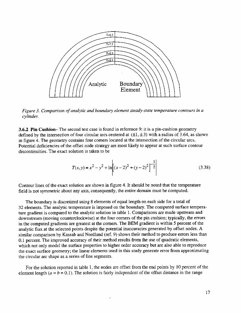
Figure 3. Comparison of analytic and boundary element steady-state temperature contours in a
cylinder.
3.6.2 Pin Cushion- The second test case is found in reference 9; it is a pin-cushion geometry
defined by the intersection of four circular arcs centered at (+1, + 3) with a radius of 3.64, as shown
in figure 4. The geometry contains four comers located at the intersection of the circular arcs.
Potential deficiencies of the offset node strategy are most likely to appear at such surface contour
discontinuities. The exact solution is taken to be
T(x,y) = x 2 - y2 + ln[(x - 2) 2
1
+ (y - 2) 2 ]-2 (3.38)
Contour lines of the exact solution are shown in figure 4. It should be noted that the temperature
field is not symmetric about any axis, consequently, the entire domain must be computed.
The boundary is discretized using 8 elements of equal length on each side for a total of
32 elements. The analytic temperature is imposed on the boundary. The computed surface tempera-
ture gradient is compared to the analytic solution in table 1. Comparisons are made upstream and
downstream (moving counterclockwise) at the four comers of the pin cushion; typically, the errors
in the computed gradients are greatest at the comers. The BEM gradient is within 5 percent of the
analytic flux at the selected points despite the potential inaccuracies generated by offset nodes. A
similar comparison by Kassab and Nordlund (ref. 9) shows their method to produce errors less than
0.1 percent. The improved accuracy of their method results from the use of quadratic elements,
which not only model the surface properties to higher order accuracy but are also able to reproduce
the exact surface geometry; the linear elements used in this study generate error from approximating
the circular arc shape as a series of line segments.
For the solution reported in table 1, the nodes are offset from the end points by 10 percent of the
element length (a = b = 0.1). The solution is fairly independent of the offset distance in the range
17

0.5
0.0
-0.5
I
-1.5
Figure 4. Pin-cushion geometry and analytic temperature contours.
Table 1. Comparison of analytic and BEM temperature gradient at the comers of the pin cushion
test problem
Point Analytic 0T/0n BEM o'-T/oan IErrorl Percent error
Comer 1 upstream
Comer 1 downstream
Comer 2 upstream
Comer 2 downstream
Comer 3 upstream
Comer 3 downstream
Comer 4 upstream
Comer 4 downstream
1.1959 1.1758 0.0201 -1.68
0.9494 0.9094 0.0400 --4.21
-1.2495 -1.2489 0.0006 -0.05
-1.1423 -1.1280 0.0143 -1.25
0.9735 0.9501 0.0234 -2.36
1.6489 1.5978 0.0511 -3.10
-0.6427 -0.6370 0.0057 -0.89
-0.8186 -0.8151 0.0035 -0.43
0.01 < a,b < 0.25. In general, experience has shown that a = b = 0.1 is the most reliable offset value;
all the results reported herein are computed using a 10-percent nodal offset. Also, the integral trans-
forms are computed using 16-point Gaussian quadrature to verify the exact integration equations
outlined previously. The gradient values generated using Gaussian quadrature prove to be within
18

4 significant digits of the exact integration results. Additionally, the interior temperature field is
computed based on the surface solution. Temperature contours compare within the plotting accuracy
of figure 4.
The spatial accuracy of the algorithm is measured by computing an error norm for successive
increases in the number of elements. The L2 error norm is shown in figure 5 as a function of the
number of boundary elements for both the boundary gradient and the interior temperature. The error
norms of figure 5 are normalized by the respective values of the error using 16 elements. The results
show the calculation of the boundary gradient to be first-order accurate while the computation of the
interior temperature is second-order accurate. This result is consistent with the accuracy of linear
elements employed in the finite element method.
0.1
0.01o(2)
0.001 ........ i ....
10 100
Number of Elements
Figure 5. Computed error of pin-cushion solution.
3.6.3 Nonconvex Polygon- The final case is a nonconvex polygon, also extracted from reference 9.
The geometry, which is shown in figure 6, is designed to test a range of comer angles. Also shown
in figure 6 are contours of the exact solution, given by
T(x,y) =sin(x)cosh(y) (3.39)
The boundary is discretized using 26 elements matching that of reference 9. The analytic tempera-
ture is imposed on the boundary. A comparison of the computed boundary temperature gradient is
given in figure 7. The abscissa of the plot is surface length starting at (x, y) = (1,1) and proceedingcounterclockwise around the domain. Also displayed are the grid point locations. The discontinuities
in the gradient values result from the discontinuous change in the surface normal between sides of
the polygon. As seen in figure 7, the computed temperature gradient is within 5 percent of the
19

2.5
2.0
1.5
1.0
0.5 1.0 1.5 2.0 2.5 3.0 3.5
Figure 6. Nonconvex polygon geometry and analytic temperature contours.
VToh
0
-2
-4
I I I
-- Analytic.... BEM
• Grid Points
.O
..°
'x0 1 2 3 4 5 6 7
Surface Length
Figure 7. Comparison of analytic and computed temperature gradient for nonconvex polygon.
20

analytic value on the boundary except at the comer points. The worst comparison is at the 90 ° comer
at (x, y) = (2,1). It is unclear why the maximum error occurs at this location. The solution is not
particularly ill-behaved at the comer, suggesting that the effect is geometry governed. It is believed
that this result is particular to the offset node strategy. In reference 9, the error at the comers corre-
lated to the turn angle with the 117 ° comer at (x,y) = (2,1.5) showing the greatest error; no such
correlation is found in the solution shown in figure 7. In any case, the efficacy of the solution
procedure is demonstrated. Finally, although not shown but worthy of mention, contours of the
interior temperature field compare to the analytic solution within the plotting accuracy shown in
figure 6.
4 Transient Boundary Element Algorithm
The development of the boundary element method for transient heat conduction follows the same
path as the steady-state presentation given in Chapter 3. In principle, the procedure is the same as the
steady-state, however, the mathematics are ubiquitous, and the general procedure is easily obscured
by the mathematical details. Referral to Chapter 3 may illuminate Chapter 4.
4.1 The Boundary Integral Equation
The derivation of the boundary integral equation commences with the transient heat conduction
equation expressed in terms of the thermal diffusivity given by equation (2.9) and repeated as
follows:
rgT o_V2 T = 0 in _ (4.1)&
with time-varying boundary conditions given by
T = T(t) on F1 (4.2a)
a_ = _(t) on 1"2 (4.2b)
The transient temperature field is split into an initial temperature field, Tl , and a perturbation
temperature, T'. The relationship expressed in terms of functional dependence is
T(xj,t) = T'(xj,t) + TI(Xj) (4.3)
Furthermore, it is assumed that the transient calculation is computed from a steady-state initial
condition, i.e.; V2T1 = 0. Accounting for these relationships, equation (4.1) becomes
aT" aV2T" = 0 in f2 (4.4)at
21
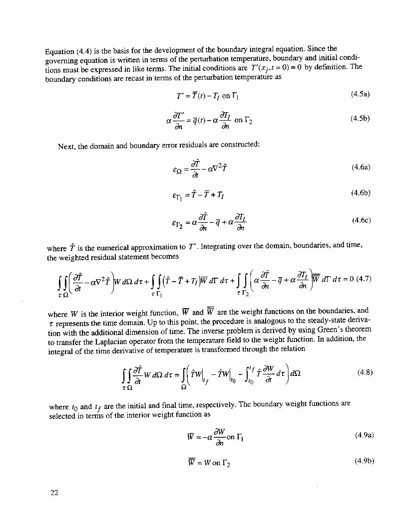
Equation (4.4) is the basis for the development of the boundary integral equation. Since the
governing equation is written in terms of the perturbation temperature, boundary and initial condi-
tions must be expressed in like terms. The initial conditions are T'(xj, t = 0) = 0 by definition. The
boundary conditions are recast in terms of the perturbation temperature as
T' = T(t)- TI on F1 (4.5a)
a_ _(t)- a--_ on F2(4.5b)
Next, the domain and boundary error residuals are constructed:
o_ aV2_. (4.6a)8_ = --_- -
eF1 = T - T + T1 (4.6b)
arler2 = a-g- + a-
(4.6c)
where 27 is the numerical approximation to T'. Integrating over the domain, boundaries, and time,
the weighted residual statement becomes
d'r = 0 (4.7)
where W is the interior weight function, W and _ are the weight functions on the boundaries, and
"t"represents the time domain. Up to this point, the procedure is analogous to the steady-state deriva-
tion with the additional dimension of time. The inverse problem is derived by using Green' s theorem
to transfer the Laplacian operator from the temperature field to the weight function. In addition, the
integral of the time derivative of temperature is transformed through the relation
II______ Wd_gdT 7"W[tf-7"weVto-Jt 0 ---_-dT d_-_
vf_
(4.8)
where to and tf are the initial and final time, respectively. The boundary weight functions areselected in terms of the interior weight function as
-- d-W (4.9a)W = -a--_-- on r 1
= W on F 2 (4.9b)
22

Furthermore,thenotationisconsolidatedthroughthevariablechangegivenby
_7_overf2 andonF27 -i
[T-Tt onrl(4.10a)
-_-a aT! on[ & r2
(4. lOb)
After the application of Green's theorem, the substitutions of equations (4.8 through 4.10), and some
algebra, the weighted residual statement becomes
rF vF
(4.11)
In order to remove the second domain integral, the weight function for the transient equation,
denoted as W tr, is selected to satisfy the following:
a_vtr t- otV2W tr = -5(r)f(t) (4.12)&
The right-hand side parameters of equation (4.12) are Dirac functions,'which represent a unit
impulse forcing function in space and time. In addition, Wrobel and Brebbia (ref. 10) have shown
that
(4.13)
Applying equations (4.12 and 4.13) to equation (4.11) yields the transient boundary integral
equation, given by
~ awtr
f_lzt/tr[ dff2+CpT"p-O_IIwtr-_-dI'dT+aIIT"----_dr'dT=O-j ,to
f_ vF vF
(4.14)
Other than the domain integral at t = t0, the transient boundary integral equation is identical in form
to the steady-state boundary integral equation (3.14). The differences are the weight function, the
additional dimension of time, and the presence of the domain integral, which appears to prevent
23

boundary-onlydiscretization.Nevertheless,thenumericalmethodologyis identicalto thesteady-statealgorithm.Moreover,it is shownin Section4.3 thatthecalculationof the domain integral canbe circumvented to recover the boundary-only character of the algorithm. Before that analysis, the
transient fundamental solution is introduced.
4.2 Fundamental Solution for Two-Dimensional, Transient Heat Conduction
The fundamental solution satisfying equation (4.12) is given by
-r2 1wt r = 1 exp H(tf - t)
4rCOt(tf - t) 4a(--_f'- t)(4.15)
where H(tf - t) is the Heaviside function. The fundamental solution is singular when r = 0 and
t = tf. The directional derivative is given by
I _/.2d-W tr _ -(7 • fi) exp 40_(-Tf- t)o3n 8_0c 2 (tf - 02
H(tf - t) (4.16)
Both the fundamental solution and its directional derivative are functions of r and ( tf - t ); i.e.,
W tr = wit(r, tf - t). This functional dependence is important in the development of the time-step
procedure presented in the next section.
When computing the transient integrals, it is convenient to transform the fundamental solution to
normalized coordinates. The spatial coordinate is mapped to the parameter _ previously introduced
in Chapter 3. Recall that the distance function, r, is expressed in terms of 4. Time is transformed
into the coordinate 7/, which originates at the source time level, t f, and is scaled by the time
interval ( tf - to). The transformation is backward in time and is given by
tf - tr/- (4.17)
tf - to
The transform variable r/ranges from 0 at t = tf to 1 at t = t0. The fundamental solution and itsderivative are written in terms of the transformed variables as
wtr (_,l"],t f -to) =47rot(t f - tO)r1
( -r2({)
exp[ 4o_(-_f _- _O)r/) H(rl(tf -to))(4.18)
ogwtr(_,O, tf-t o ) -(F._) ( -r2(_) .)
_ ) n(rl( tfOnrl = 8l_z2(tf--'_o)2rl2 exP_4offtf-to)rltO)) (4.19)
24

The fundamental solution and its derivative are functionally dependent on _, 77, and the time
interval (tf - tO) from the temporal coordinate transformation.
4.3 Time-Step Procedure
Consider the boundary integral equation expressed over the temporal domain from tO to tf,
given as
N
-f _vtr(r, tf-t) d_-2+CpT"p -6_fff _wtr(r, tf-t)-_dFd'c
f2 to F
+ o[ftf t ~ o3wtr(r, tf - t)"It0 JT _ dFd't" =0
F
(4.20)
The functional dependency of the fundamental solution is included in the previous expression to
accentuate the source point, which is always located at tf. After the boundary is discretized, the
integral equation can be written in terms of coefficient matrices of the temperature and gradient
vectors. The form of the equation is dependent on the order of the temporal accuracy. For discussion
purposes, the temporal accuracy is assumed to be O(1) in order to simplify the equations. In practice,
the algorithms presented in this paper employ a linear interpolation function, the details of which are
presented in Sections 4.4 and 4.5. As before in the steady-state analysis, the notation is switched to
matrix form for compactness. Equation (4.20) becomes
Dj(Tj(to),t f - to) + Hjk(t f - to)Tj(t f ) + Gjk(t f - to)Qj(t f) = 0 (4.21)
where Hjk and Gjk are the coefficient matrices, identical in function to those of equation (3.16),
and Dj is a vector containing the domain integral, which is a function of the temperature field at
tO and the time interval (tf - to). The parenthetical expressions after Tj and Qj indicate time level,
while those after D j, l-ljk, and Gjk denote functional dependency. As will be shown later, thetemporal portion of the integral transforms admit analytic solutions that are functions of the time
interval ( tf - tO). Thus, the coefficient matrices D j, I-Ijk, and Gjk are denoted as functionallydependent on the time interval. Although not explicitly indicated, the matrices are also functions
of the geometry.
Wrobel and Brebbia (ref. 10) present two methods for advancing the boundary integral equation
in time. In the first approach, the time integration is initiated from the previous time step; this pro-
cess requires domain integration and, consequently, a domain grid. In the second approach, domain
integration is avoided by initiating the integration for every time step from to . The two approaches
compel different storage and computation strategies. Both methods are now discussed.
Let the time domain be divided into intervals with the time at the end of each interval denoted by
tm . In the first approach, the solution from tm_ 1 tO t m is given by
25

Dj(Tj(tm_l ),tm - tm_l ) + Hjk(t m - tm_ 1)Tj(tm) + Gjk(t m - tm_ 1)Qj(tm) = 0 (4.22)
Equation (4.22) is essentially a rewrite of equation (4.21) with a change in the time interval from
(tf -to) to (t m -tm_l). To advance the solution in time, the coefficients in Hjk and Gjk arecomputed based on the local time step, (t m - tin_ 1). The domain integral is computed based on the
temperature field at the previous time step. For varying values of the time step, Hjk and Gjk need
not be retained. If the time step is constant, however, the coefficient matrices are a function of a
fixed geometry and a fixed time step; therefore, they can be computed once and stored. This
procedure is very efficient except for the requisite domain integration.
In the second method, domain integration is avoided by writing equation (4.21) from t O to tm .
At the initial time, Tj (t 0) = 0 by definition (recall that Tj contains the perturbation temperature andnot the absolute temperature, which can be nonzero), consequently, the domain integral is zero.
Equation (4.20) becomes
m m
ZHjk(tm - ti_l)Tj(ti) + ZGjk(tm - ti_l)Qj(ti) = oi=1 i=i
(4.23)
The summation appearing in equation (4.23) results from dividing the time integral into intervals
corresponding to the time-step distribution. The integrals are computed using the transient history
of the dependent variables. The coefficient matrices must be calculated for every combination of
( t m - ti) for every time step. For example, assume the solution has been computed up to time t1.
To advance the solution to time t2 , coefficient matrices must computed for time intervals of (t 2 - to)
and (t 2 - tl). The terms of the first summation of equation (4.23) are
2
Z I'Ij k (t2 - ti-1 )Tj (ti) = I-Ijk (t 2 - t0)Tj (t 1) + I'Ijk (t 2 - t 1)Tj (t 2 )i=1
(4.24)
At the next time step, the matrices must be computed for time intervals of (t 3 -to), (t 3 -tl), and
( t 3 - t2). The terms of the first summation are
3
Z I'ljk (t3 - ti-1 )Tj (t i ) = I'Ijk (t 3 - t o )Tj (t 1) + I'Ijk (t 3 - t 1)Tj (t 2 ) + I-Ijk (t 3 - t2 )Tj (t 3)i=1
(4.25)
Thus, for a calculation of mma x nonuniform time steps, mma x (mma x + 1)/2 coefficient matrices
must be computed to cover the possible combinations of ( tra - ti) for 0 < i < m and 1 < m < mma x.
In general, the value of ( tm - ti) need not repeat itself, therefore, I-Ij, ( tm - ti) and G jk (tin - ti ) are
never repeated. Storage is minimal because only one matrix at a time is needed, but the amount of
computation is high.
Matters are simplified somewhat for a constant time step because the number of matrix calcula-
tions is reduced to mma x • Furthermore, the matrices, which are a function of integer multiples of the
time step, are computed once and stored. For a constant time step, equation (4.23) becomes
26
m m
E Hjk((m - i+ l)At)Tj(ti) + E Gjk((m - i + 1)At)Qj(ti ) = 0i=1 i=1
(4.26)
Unfortunately, because the origin of the source point is always at tm , the matrix vector multiplica-
tions of Itjk((m - i + 1)At)Tj(ti) and Gjk((m - i + 1)At)Qj(ti) are never repeated. For example, at
the second time step, Hjk(2At) is multiplied by Tj(t 1), while at the next time step it is multiplied
by Tj (t 2). Consequently, there is no possibility for computational and memory savings by storingintermediate vector-matrix multiplication results.
Wrobel and Brebbia (ref. 11) recommend the first method, which requires domain discretization,
for most applications. Although the first method has the overhead of the domain integral, the effi-
ciency is independent of the number of time steps. In the second method, on the other hand, the
efficiency decreases as the number of time steps increases; the efficiency of the second method
quickly falls below that of the first as the number of time steps is increased. Yet, it is the author's
opinion that the primary benefit of using the BEM is the boundary-only discretization. If the domain
must be discretized, perhaps the finite element method is better suited since it is conceptually less
complicated and is amendable to increases in fidelity such as modeling nonlinearity. In light of this
philosophical perspective, the transient algorithm presented in this paper employs the second method
to exploit the advantage of boundary-only discretization. Of course, these brush strokes are broad,
and certainly there may be compelling reasons to use a BEM that requires domain discretization. It
has to be the engineer's discretion when to use a wrench and when to use a ratchet.
4.4 Element Shape Functions and Integral Transforms
This section presents the numerical details of the transient boundary element algorithm. The
transient algorithm retains the features developed for the steady state: a linear boundary element
shape for efficient coupling with CFD, variably offset nodes for unique definition of the node
normal, and a linear spatial distribution of the dependent variables. These components are
incorporated into the boundary-only time-step procedure introduced in the previous section. The
interpolation function is modified to linearly approximate the dependent variables over space and
time. The interpolation function is inserted into the boundary integral equation to derive the integral
expressions. The integral transforms over time and space do not admit a complete analytic solution
except in the instance of a singularity. The integral transforms of the singular and nonsingular types
are addressed separately.
The boundary integral equation for the boundary-only time-step procedure is given as
tm _ tm . o3wtrCpTp-all Wtr(r'tm-t) On
t o F t0F
(4.27)
where tm is the time at which the solution is to be computed. It is assumed that the solution has
been previously computed up to time tm_ 1. As outlined in the previous section, the domain integral
vanishes because the integration always commences from tO. The time intervals are not necessarily
constant; that assumption will be made later in the derivation. The boundary is divided into elements
27

and the time integration is divided according to the time-step distribution to yield the double
summation in the boundary integral equation,
m ti ~i rn ti
CpZp-OtE _ E_wtr(r'tm-t)_ dFd_+O_E _ E_i°wtr ---_(r,t m - t)dF d't = 0
i=lti_l e Fe i=lti_l e Fe
where Te is the distribution of T over element e from time ti_ 1 tO t i , and oT/"//On is defined
likewise. Isolating an individual term from each of the double summations reveals the two integral
transforms that comprise the crux of the numerical solution,
(4.28)
t) dl-" dr (4.29a)
_il_wtr(r, tm-t)--_-dT'dT;
re
(4.29b)
The solution of the integrals is different for singular and nonsingular integrands. In the nonsingular
case, a mixed analytical-numerical solution is prescribed. In the singular case, an analytic series
solution is derived.
4.4.1 Nonsingular Integrals- In this section, the equations for the integral transforms of equa-
tions (4.29) are presented for the case of a nonsingular integrand. As will be shown, the temporal
integration admits an analytic solution, whereas the spatial integration is perfo.rmed numerically.
First, the interpolation function of the dependent variables is developed. Let _e represent the distri-
bution of either T or dT/dn over element e from time ti_ 1 to t i. The four-point basis function is
given as
1 {Zi[(l_b_4)_e,l(ti_l)+(__a)_)e,2(ti_l) ](1 - b - a)
+ (1- Zi)[(1- b - _)_e,l(ti)+ (4 - a)_e,2 (ti)]}
(4.30)
where Zi is a local time variable that ranges from 1 when t = ti_ 1 to 0 when t = t i. The parenthetical
expressions after _e,j indicate time level. The subscripts 1 and 2, first introduced in the steady-state
interpolation function, indicate the two nodes of each element. Equation (4.30) is a bilinear function
over space and time expressed in terms of the local time variable, Zi, and the spatial transform
variable 4- The interpolation function is more suitably expressed in terms of the global time
variable r/ given by equation (4.17), which in this usage ranges from 1 at t = tO to 0 at t = tm .
Equation (4.30) becomes
28

_ie = 1 1 { _(tm _ti)[(l_b)_e,l(ti_l)_a(ge,2(ti_l)](1 - b - a) (t i - ti_ ! )
+(t m -ti-1)[(1-b)Oe, l(ti)-aOe,2(ti)]
+ (t m -to)[(1- b)Oe,l(ti_l)- a_e,2(ti_l)-(1- b)Oe,l(ti)+ aOe,2(ti)]r /
+[(t m -ti)(@e,l(ti_l)--Oe,2(ti_l))--(tm --ti-1)(_)e,l(ti)--_,2(ti))]_
+('m +ae,:(,,-,)+ae,,(t/)-ae,:(t/)).} (4.31)
Since the interpolation functions are expressed in terms of _ and 77, they are combined with
the transformed fundamental solution given by equations (4.18) and (4.19). The integrals of
equations (4.29) are mapped into (i-r/) space to yield
W tr r
Stti I _i °_¥tr(r'tm-t) dFd'C=On(tm---to)drT(ti)lefr/(//-1 ) f 17"e(_' r/)egO0 ( (¢)'r/'tm-tO) dCdr/Oni-1
re
(4.32a)
Ifi_l I wtr (r, tm - t)-_ -dr'd'C -
re
-i
le fO(ti-1)I1wtr'r"" -to) 3Te (¢' r/) dCdr/(t m --- tO) dr/(ti) 0 _ (_)' r/' tm On
(4.32b)
The integrals are functions of _, 77, the known boundary solution for t < ti_ 1, the boundary
conditions, and the unknown quantities at t = ti. The expression does not admit analytic solution
over space and time, but manipulation of the temporal integral is fruitful.
The multiplication of the fundamental solution (eqs. (4.18) and (4.19)) and the interpolation
function (eq. (4.31)) produces three core time integrals of the form
frT(ti- 1)+ expl 4a_-) Idr/ for k = 0, 1, 2
Jrl(ti ) to )(4.33)
The values of 77 at the limits of integration are found by applying its definition given by
equation (4.17). Furthermore, the time integral is split into two parts to yield
tm -ti-1 2 "_
S r/(ti-l) 1 (-r2(_) ]dr/= f tm-tO lexp( --r (__.)) Jrl(ti) r/k exp/4a_-_m 7/0 ) do 77 _40tr/(tm-tO)
tm - t_______i )_ I;m-t0 +exp -r2(_) .40_r/( tm - tO)fork=0,1,2
(4.34)
29

Both of the integrals on the right-hand side of equation (4.34) are of the same form, and a general
solution appears to be possible. Yet, the time difference in the exponential function is (t m -t O) whilethe time difference in the numerator of the upper limit of integration is ( tm - ti); this fact suggests
that the integral must be computed for all combinations of (t m - ti) and (tm - t0) for 0 < i < m and
1 < m < mma x. Fortunately, the integrals can be transformed to yield standardized integration limits
of 0 < r/< 1. The results for each of the three types of integrals are
I;m-t0 exp( -r2 ) tm - ti tl ( -r2tm-ti dr/= _ exp --- )dr/4a(t_ --t 0 )7"/J tm -t o Jo ( 4ot(t m -t i )17(4.35a)
tm-ti'( 2 ) =rllexp/. -d ,ldr/ (4.35b)ftm_tO lexp[ --r dr/dO 17 _,4a(t m - to)r� aO 77 _.4a(t m - ti)r/)
tm-t-----L+l-r2)tm-tofll¢-r2 lexp..... exp --- dr/ (4.35c)
dr/ jor/2 _4a(tm_ti)r/; m-tO 40_(t-_ _ t0)r / tm - ti
Notice that the integration limits and the time difference in the exponential function have been
standardized. Combined with the spatial integration, six component integrals result. The integrals are
of standard form, and for a constant time step, are computed once, stored, and used repeatedly. The
six integrals are denoted by the superscript tr to distinguish them from the steady-state integrals;
they are given as
S;£e(++)I tr xp dr/1,i =
I tr rl 1,1. ¢_ri2(_)) d_2'i : J0J0qexp t 7/" dr/
itr = fl fl lexpf ]dr/3,i d0J0r/ [ /7 )
I lr fl fl exp(-r/2__(¢)Jar/d 4,i = JOdO r/ _. 17 J
it r r 1 1"1 1 (-r/2(_) / d{5,i = jo£Texpt -_ dr/
lt6r'i : JoJoTeXpt de
(4.36a)
(4.36b)
(4.36c)
(4.36d)
(4.36e)
(4.36f)
3O

where
ri2 (_) - r2 (_) (4.37)4ot( tm - ti )
Furthermore, the time integration is performed analytically to yield
1 2Itr=l,i IoE2(r/ (_))d_
(4.38a)
2,i _E 2 ri2(_) d_ (4.38b)
1 2
Itr=3,i f0El(r/ (_))d_(4.38c)
l_r,i = _E 1 r/2(_) d_ (4.38d)
I 'r fl ,I exp(ri2(_))d_5,i = dO r/z (_)
(4.38e)
6,i = exp _) d_ (4.38t)
where E1 and E2 are exponential-integral functions whose expressions are given in reference 12. The
integration over _ is performed numerically using Gaussian quadrature with the distance function
given by equation (3.21).
Summarizing up to this point, interpolation functions that are linear in both time and space are
given for the dependent variables. The interpolation functions are expressed in terms of the trans-
form coordinates _ and 7/. The multiplication of the interpolation functions to the kernels of the
integral transform (i.e., the weight function and its derivative) yield three core temporal integrals as
functions of r/. The limits of integration and the time difference in the exponential term of the core
integrals are standardized. These three core time integrals are combined with the spatial integration
to produce six component integrals in space and time. The temporal integration is performed analyti-
cally and the spatial integration is computed using Gaussian quadrature. Utilizing the definitions of
the six integrals, the expression for the integral transforms of equations (4.29) are
31

le 1R. -(tm ti) (l-b)= . - (ti_ 1 ) - a (ti_ 1 )
4re(1 - b - a) t i - ti_ 1i=1
+ (1-b)--_-(ti_l)-a--_(ti_l)-(1-b)-_-_-(ti)+a--_(ti)[(tm-ti-1)I{, r-l-(tm-ti)l_,r]
+{(tm-ti)[--_-(ti_l)--'_-_-(ti-1)l-(tm-ti-l)I-_-(ti)--'_(ti)l}(l_ri-l-It4ri)
-1 ?_ O_e,1 °_e 2 ~ _a___(ti _(tin trLi-1 ) 2,i-1
(4.39a)
= 81r--_---b _ a) _ t i - ti_l ' "
11[<i_1"r+(tm-ti-1)[(1-b)Te,l(ti)-aTe, 2(ti) (tin _'_-/_1)(tm-t i )
+[(1- b)7"e,l(ti_l)- aT"e,2(ti-1)-( 1- b)Te, l(ti ) + aTe,2(ti)](I_, r-1 - It3r,i)
[" ltr
+{(tm -ti)[Ze,l(ti-' )- _re,2(ti-1)]-(lm-ti-1)[ _i'e'l(ti)- Ze,eCti)]}/L(',_:L1)6'i-1 ,,r]6,i
(tm - ti)
G_ aTe 2(ti)] It4ri 1- Itr ] I+[-Te,l(ti_l)+ 7"e,2(ti 1)+ Te,l(ti)- , ( ,- 4,iJ
3(4.39b)
32

ZC ltr trNotice that the integrals 1j,r. appear in pairs of the form _ 1 j,i-1 -c2I),i) because of the splittingof the integration limits shown in equation (4.34). Also, terms of the form (t m - ti) result from the
standardization given by equation (4.35). The equations are tedious and the notation is abstruse, yet
the concept is straightforward and should not be lost in the details of the algebra. The equations are
obtained simply by multiplying the interpolation function by the transform kernels.
Equations (4.39) are valid for any distribution of the time steps. Recall, though, that if values of
tm are selected arbitrarily, then the integrals 1_,r must be calculated for all possible combinations of
( tm - ti) for 0 < i < m and 1 < m < mrnax. If the time step is constant, however, then ( ti - ti_ 1)
becomes At and (t m - ti) becomes an integer multiple of At. The integrals need to be calculated
only mma x times. Furthermore, because the influence coefficients are a function of a constant At,
often only one matrix inversion is required for all time steps. Extracting out At, the integrals overtime are
m t. i
f f: wtr (r, tm - t)-_ dT.dF =Ie
4n:(1 - b - a)
+(m-i+ I)(l-b)CT_f'l(ti)-ona--_(ti) (l_ri_1- Itr3,i)
+I(l-b)-_-(ti_l)-a_(ti_l)-(l-b)-_-(ti)+a--_(ti)][(m-i+l)l_r,i-1-(m-i)l'r,i]
°_el °_e,l
+{(m "i)[----_--(ti_l)--_(ti_ 1°_e'2 )]-(m-i+ 1)[--_---(ti) ---
+
(4.40a)
33

V
onwtr (r, tm - t) -( _ • n )le [
f2I'i; i=1 ti-1 N 81"g_((_--V-- a)i=1
[- ltr I tr ]
+(m-i+ 1)[(1-b)7"e,l(ti)-aTeg(ti)B] '5,i-1 5,i J' IJL(m -- i + 1) (m- i)
+[(l_b)_.e,l(ti_l)_a_.e,2(ti_l)_(l_b)_.e,l(ti)+aTe,2(ti)](l_,i_ l- tr - Itr3,i )
._ I tr
+ {(m- i)[Te,l(ti-1) - ]'e 2(ti-1)] -(m- i + 1)[7"e l(ti )- ]'e 2(ti)]}l, 1", , , L_rn - )
,,r]6,i
(m - i)
+[_Te,l(ti_l)+ Te,2(ti_l)+ Te, l(ti)-aZe,2(ti'l[l trl]_4,i-1 - 1tfi) ]
(4.40b)
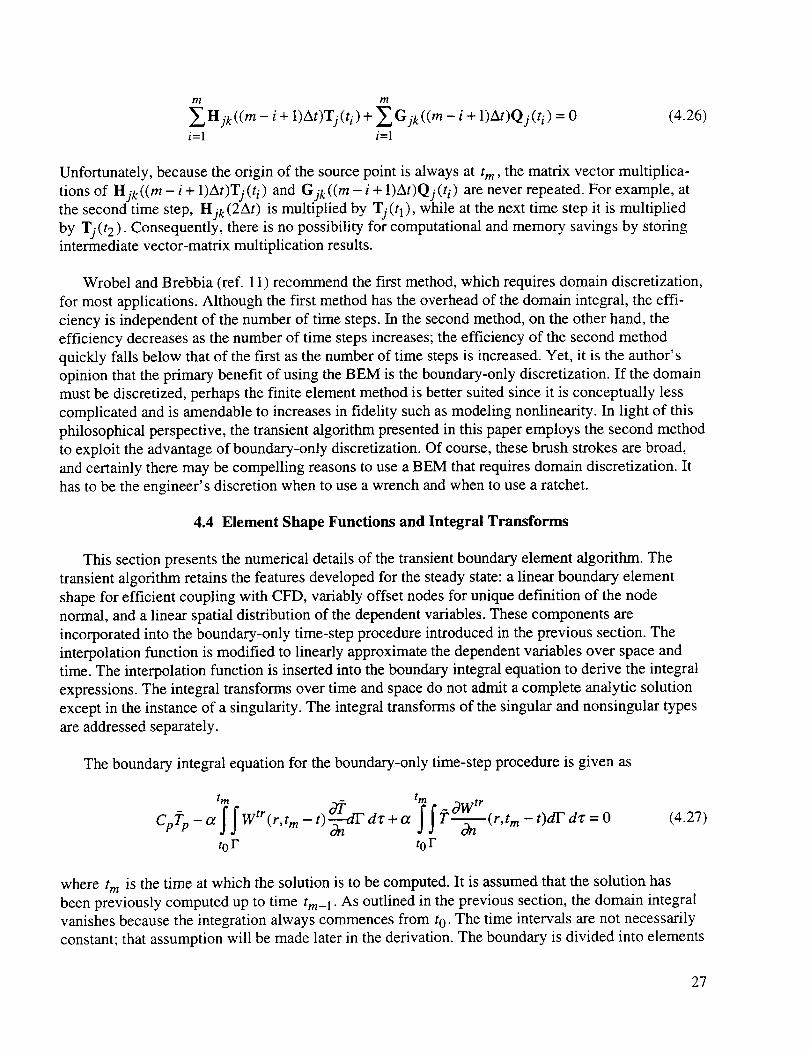
4.4.2 Singular Integrals- The previous section develops expressions for the integral transforms
when the integrand is nonsingular; this section presents expressions for the integral transforms for a
singular integrand. The singularity occurs when the source point lies on the element defining the
path of integration. Because the distance function simplifies in this orientation, the integral transform
admits a complete analytic solution over time and space. Furthermore, since the source point lies
along the path of integration ( _ • h = 0), the integral of equation (4.29a) is zero.
The singular integral requires an interpolation function for 3"T//3n. It is convenient to redefine
the spatial transformation such that the origin lies on the source node point. The range of the trans-
formation becomes -a < _ < 1 - a, where a is the offset distance of the source point. The notation
in this section is analogous to the notation used for Orientation 3 of the steady-state transform of
Section 3.5.3. Letting subscript p denote the source point and q denote the other node point, the
interpolation function for O_et/_ is
3n (1-b-a) Zi (1-b-a-_) (ti_l)+_ (ti-1)
(4.41)
In the new transformation, the second node point is located at _ = 1 - a - b.
34

Similar to thederivationin theprevioussection,multiplicationof the interpolationfunctiontothetransformedfundamentalsolutionproducescomponentintegralsovertime andspacelike theintegralsof equations(4.36).With therevisedspatialtransformation,thecomponentintegralsare
I tr fl-afl (_ri_)ldr/d _ (4.42a)1,i = a-a jgxp_,
Itr a d_ (4.42b)2,i = exp dr/
It r I"l-a fll (--r/2(_))_3,i=La j0-_exp_ _ jar�de (4.42c)
I tr = fl-afl _ exp(_r/2_.(¢ )/dr/d_ (4.42d)4,i d-a J0 77 \ /7 J
Because only one of the integral transforms is nonzero, only four component integrals are needed (as
opposed to the six component integrals for the nonsingular case given by equations (4.36)). Each of
the four integrals admits an analytic solution over time and space. The derivation of I_,ri is presented
in detail as an example. The other three are derived similarly, but, for brevity, only the final expres-
sions are given. With the distance function explicitly expressed in terms of _ I tr, 1,i is given by
I tr I'1 l'l-aex (-fli_2 _ d_ (4.43)'.i:JoJ- 77 ) dr/
where
fli - le (4.44)4a( tm - ti)
The integral is singular at the origin. An additional transformation to polar coordinates allows
the Cauchy principle value to be computed in the limit as the radius goes to zero. The domain is
divided into two regions along the r/ axis. A separate polar coordinate transformation is prescribed
for each region, as shown in figure 8. In each region, the limits of integration are easily determined
by splitting the integral in two at the comers of _-r/space; i.e., at (_, r/) = (1 - a, 1) and at
(_, r/) = (-a, 1). Both regions are transformed to polar coordinates and subdivided in two to
yield four separate integrals
35

I tr = exp Z dZ dO1,i sin 0
+ It _ fsi@O exp/-fli_cOs2 0an-I (l___la)dO _ sinO _d_dO
+fta_-t@f;-_s_exp[-/3iAsin2qt)Jo-'o \ _ _,dA,dqt
7r a • 2
+J'ta2-n_l fs_n_exp(,-fli_'sin'llIA, dZdlll)(a)JO _. cos_
(4.45)
:1i T= -/l sin _ _ = _ cos 0
77,= ,_ cos gt / 77= XsinO
gt
7=0 --
=-a _ =0 _ =l-a
Figure 8. Singular integration domain and polar transformation.
36

Theinner integrationover Z is performed analytically to yield
itr _'tan-l(l_--la)-sin20 [exp(-fli(1-a)cosO)(fli(1-a)cosO _-ll-lldOl,i = Jo t2 c0s4 0 sTn-0 jr. G
fq-_r -sin 2 0 F (-flicos 2 0/,ico, 0+1/_1]sin 2 0
ftan-l(a)-cos2 I/f F (-flisin2111_(flisin2v)l.... exp -- . +1 -1 dN+_o #sin44 t _os_J_co_ (4.46)
rc _cos2N[expl__iasi____nllf.li_iasin______.ll_l]d _+Ita2n-l(a)_2sin41//L \ cosl]/ j\ cos_
Each of the four integrals of the right-hand side of equation (4.46) is mapped to a dummy variable,
u, through separate substitutions. Letting u = tan 0/(1 - a), u = tan O, u = cot N, and u = cot N/a for
the first through fourth integral terms, respectively, yields
12E 1I 'r =-(1- a) 3 f(l---_ u--w exp + 1 - 1 du1,i Jo /_¢
-_ U2
-Jl@a _/2FexL P_'-_'-)_u-2"('-_i_(fli +1)- 1] du
- I_ _/22[exp(@2/)(5 + 1) - 11 dua
(4.47)
3 f_12 u2 1]-aJ0a -_-i2[exp(-_-L)(_+l)- du
The first and fourth integrals on the right-hand side of equation (4.47) are of the same form, and the
second and third integrals are of the same form. The solutions of the third and fourth integrals are
addressed with the knowledge that the solutions of the first and second are obtained by substitution
of (1 - a) for a. The fourth integral of equation (4.47) yields to analytic solution. Furthermore, the
solution is expanded into series form; the result is
37

au2E l l lexp a2 i (l+ll+aE2 a2 i -a__ e_ +1-, _u-- a_# a_i
11 _ (-1)kflka2k+l=_L_o (k + 2)k' +aE2(a2fli)]
(4.48)
The third integral does not readily submit to analytic solution. Nevertheless, the integrand is
expanded into series form and each term is integrable. The Cauchy principle value is found for
each term at the upper limit of integration; the result is
_u2 - " t" 11 7_ " l"k-l'_k-1-;i_-/2[exp(_)(_--_+l-I du=LimflS" ,_.-_-21)--pi- dur_3ak='--'lU_'_(k + 1)(k- 1)!
(-1)k+1,6/_ Ir= Lira 2 2k+l(2k+l)(k+2)k! -7--..> k=Ou 1
a
(4.49)
The two series expansions found in equations (4.48) and (4.49) are combined to yield
1 _.(-l)kflka2k+I _ (1)kflika2k+l 2 _.(-l)kflka2k+l
_ __ +_o__;_,--3_ _ +i)_,(4.50)
Since the two series solutions can be combined, the sum of the solutions of the third and fourth
integrals renders two terms: a series expansion given by equation (4.50) and an exponential integral
function. The first and second integrals combine in like fashion. Summing all four integrals, the
solution for I tr1,i is
a 2 2 (-1)kflk[ (1-a)2k+l+a2k+l ]
l{ri=_-E2((1-a)2fli)+ "E2(a fli)+3k= 0 (2k + 1)k!(4.51 a)
Similar derivations for ! tr I tr I tr2,i, 3,i, and 4,i yield
i tr (1-a)2E2((1-a) 2 ] a2E ra2a/a i)+ 1 Z_ (-1)kflk[(1-a)2k+2k=0
_ a 2k+2 ](4.51b)
38

_1,k a,2k+1 2k+ ++ (4.51c)
,tr= _z_.l I(1 - E2(( 1 - a)2 fli))-(1- E2((1- a) 2 fli ))]4,i Z#i L\
(4.51d)
The series shown in equations (4.51) are convergent for fli < 1. In practice, the element is broken
into subelements such that the length of the subelement containing the singularity yields fli = 0.8.
For fli = 0.8, the series converges to sufficient accuracy in six terms. The remaining subelements are
nonsingular and are integrated numerically as in the previous section.
When a = 0, the expressions of equations (4.51) are undefined; however, the limiting form is
found to be
it r 2 '_ (--l) kflk
1,i = E2 (_i) + -_ k___(2-_" 1-'_!(4.52a)
1E la _+ 1 _-, (-1)kfl kI tr"-'; 2 k_ i ] _ Z-, ' (--_+ i-_.2,i ="e _ k=0 _ "
(4.52b)
1)k kitr 1- g2(fli) _" !=1)_ ]_t
3,i - fie t- k_-_(2k + 1)(k + 1)!
(4.52c)
Itr (1- E2(fli))
4,i - 2fl i
(4.52d)
The analytic expressions given by equations (4.51) and (4.52) are compared to numerical integration
in figures 9 through 12. The numerical integration is performed using two-dimensional Simpson's
Rule with 109 functional evaluations. The analytic expressions are seen to reproduce the numerical
values over a range of fli and a. Recall that the analytic expressions are not employed for /_i > 0.8
tO ensure convergence of the series solution. The only discrepancy between the analytical and
numerical solutions is for l_ri at small values of/3 i , as shown in figure 11. This difference is caused
by error in the numerical solution; the Simpson integration requires extremely fine spacing to
resolve the singularity of the integrand.
39

trl,i
0.9
0.8
0.7
oo!0.5 t
10 -4
.... O---Numerical a=O.O I \ __\
a=01I \5'....m---Numericala=0.11 k k.
Analytical a=0.2 [ _ m
A, Numencal a=-0.2 [ \
h i ...... I , , , , .... I , , , ,,,,,i .......
10 .3 10 -2 10 -1 10
Figure 9. Comparison of analytical to numerical solution of transient, singular, component
integral I tr1,i.
tr2,i
0.50
0.45
0.40 i0.35
0.30
0.25
0.20
0.15
10 4 10 .3 10 .2 10 -I 10
E
Figure 10. Comparison of analytical to numerical solution of transient, singular, component
integral I tr2,i.
40
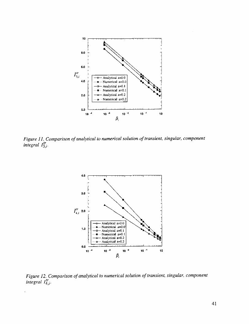
I;7i
lO
8.0
6.0
4.0
2.0
.... +"" Numerical a=O.O[ %xl,"x,_
_ NA3_Yetnic_ aago i1
Analytical a=0.2 [ m
0,0 , , , ,,,,,I + , L ..... i ........ I
10 4 10 -3 10 .2 10 .I 10
Figure 11. Comparison of analytical to numerical solution of transient, singular, component
integral I tr3,i"
4.0
3.0
I tr 2.04,i
1.0
0.0
10 4
........ I ........ i ........ i ........
.... • ---Numerical a=0.01 "_, "_'_
Analytical a=0.1 I "_,"x_
.... "-- Numerical a=0.11 "A"Q,.i_
Analytical a=0.2 I _'_
.... _,---Analytical a=0.2 I
10 -3 I0 "_ 10 "+ 10
Figure 12. Comparison of analytical to numerical solution of transient, singular, component
integral l_ri .
41

With IJri defined, the expression for the singular integral transform is
!i_=lftiwtr(r,tm-t)ti_l dzdF
le4zr(1 - b - a) i_ 1"=tt" _lti_l (1-b-a)-(tm-ti)---_--(ti-1)+(tm-ti-1) (ti) I_ri-l-I_ri)
+(1-b a) (/i-1) °_e'P(ti) (tm-ti-ll_ltrl,i-1_ _(tm _ti)l,,, ]tr]
+{(tm --ti)E-_(ti-1)---_(ti-1) --(tm --ti-1)I-_(li) °_'q (ti)])(lt4ri-l -lt4ri)
~ ] ) 2,i-1 ]r o_. o_ e O_e. __(ti) [(tin ti_l,[tr (t m ti)l_ri]+ _v-e,p (ti_l) + v'e,q (ti_l) + _,e (ti)_ a _ _ _
(4.53)
4.5 Numerical Results
The transient algorithm previously developed is tested against three analytic solutions. All three
test cases are simple one- and two-dimensional geometries for which transient analytic solutions are
found in reference 13. The first case is the temperature decay in a one-dimensional rod with an initial
linear temperature distribution. The second case is the temperature decay of a two-dimensional
plate initially at uniform temperature. Finally, the third case is a one-dimensional rod with a time-
dependent fluctuating temperature boundary condition.
4.5.1 One-Dimensional Rod- The first test case is a one-dimensional rod of length I with an initial
linear temperature profile. The initial and boundary conditions are given by
Initial conditions: T(x, t = O) = (1 - x)/l for 0 < x <_l
Boundary conditions: o3T/On(x = 0,t) = 0 for t > 0
T(x = l,t) = 0 for t > 0
The domain is discretized using 11 elements along the length of the rod and 5 elements of length 0.1I
in the second dimension. Symmetry boundary conditions are imposed along y = 0 and y = 0.5/to
simulate a one-dimensional problem. Temperature values at five select points along the length of the
domain are compared to the analytic solution in figure 13. The abscissa is time nondimensionalized
by the thermal diffusivity, a, and the length of the rod. The boundary element solution reproduces
42

0.8
0.6_=
E 0.4
[.=
0.2
.... I .... [ .... = .... [ ........ I .... I .... I
- -o - x/l=0.9 BEM
.__ + x/l=0.9 Analytic
- -G -. x/l=0.7 BEM "]+ x/1=0.7 Analytic ]
- - * -- x/l---0.5 BEM
----4--- x/l=0.5 Analytic __• _L'x__ --J'-" x/l=0.3 BEM
_. _,v',v,_ _ x/l=0.3 Analytic
• - _ '_-_"_.__ --v-- x/l=0.1 BEM J
: -.-
0 0.1 0.2 0.3 0.4 0.5 0.6 0.7 0.8
at/l 2
Figure 13. Comparison of analytical to boundary element transient temperature profiles in one-dimensional rod.
the analytic solution throughout the domain and for all time. The error, expressed as a percentage of
the difference between the analytical and numerical solutions, is plotted in figure 14. The greatest
error occurs at the initial time step; the cause of this effect is discussed in the next section. After the
initial time step, the error decays to within 0.3 percent of the analytical solution.
4.5.2 Two-Dimensional Plate- The second test case is a finite square with unit initial temperature.
At time zero, the boundary temperature is instantaneously dropped to zero. Heat then flows out of
the domain and the temperature drops to zero in the steady state. For this simulation, the boundary
is discretized using 11 equally spaced elements per side. The square ranges from (x,y) = (0,0) to
(x,y) = (l,l). Symmetry boundary conditions are imposed along x = 0 and y = 0. The temperature
is set to zero on the remaining two sides. In figure 15, the boundary element solution is compared
to the analytic solution at five locations inside the domain. The points that are plotted, although
selected for broad representation of the solution, are completely arbitrary and have no correspon-
dence to any type of interior discretization. Any other five points could easily have been selected.
Except for the first two or three time steps, the boundary element and analytic solutions are nearly
identical to plotting accuracy. The error of the solution is presented in figure 16. Similar to the
results presented in figure 14, the greatest error occurs at the initial time step. The error is slowly
rising in time past 0.2 because the error is expressed as a percentage of the analytical solution, which
is approaching zero. Thus, the percentage error is increasing even though the absolute error is
decreasing.
43
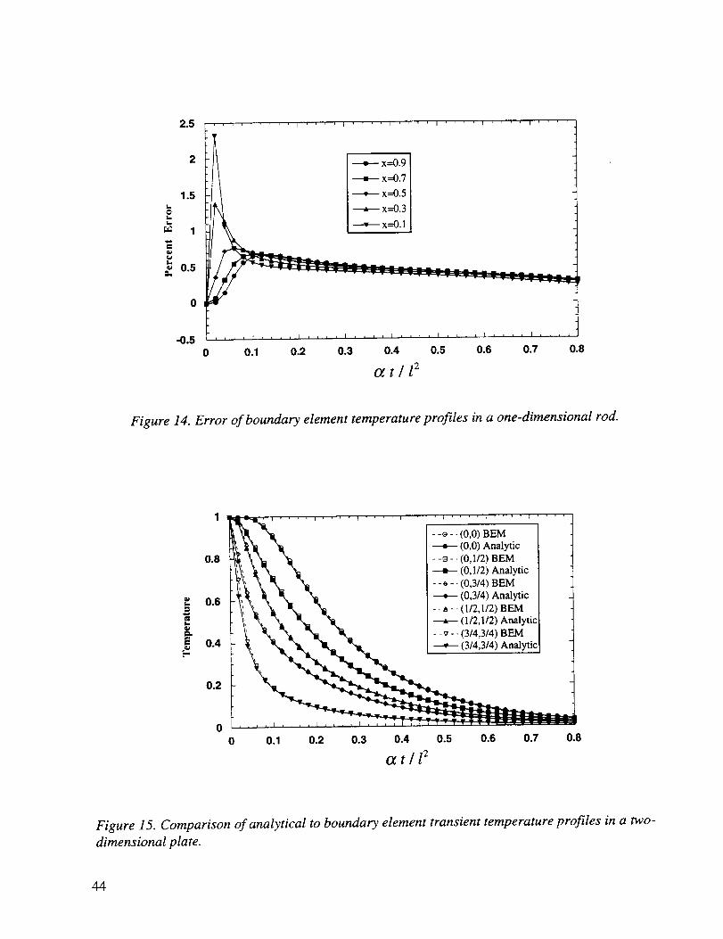
0 0.1 0.2 0.3 0.4 0.5 0.6 0.7 0.8
a t/l 2
Figure 14. Error of boundary element temperature profiles in a one-dimensional rod.
1
0.8
0.6
_ 0.4
0.2
00 0.1 0.2 0.3 0.4 0.5 0.6 0.7 0.8
a t[l 2
Figure 15. Comparison of analytical to boundary element transient temperature profiles in a two-
dimensional plate.
44

r_
12
10
8
----4'-- (0,0)
(0,1/2)
(0,3/4)
(1/2,1/2)
(3/4,3/4)
4
2
0
-2
0 0.1 0.2 0.3 0.4 0.5 0.6 0.7 0.8
at/l 2
Figure 16. Error of boundary element temperature profiles in a two-dimensional plate.
The slight deviations near time zero are explained by recognizing that the heat flux at time zero
is infinite because of the instantaneous temperature drop. Consequently, the initial temperature
gradient is computationally undefined which undermines the ability of the linear shape function to
describe the thermal gradient over the first time step. This computational obstacle is circumvented
by dropping the order of the temporal shape function over the first time step. Thus, the first time step
for the transient calculation employs a constant temporal shape function while all subsequent time
steps use a linear. As a result, the first time step has a reduction in accuracy as compared to the
remainder of the computation. The effects of the accuracy reduction, however, do not propagate intime.
4.5.3 One-Dimensional Rod with Fluctuating Boundary Condition- The final test case is a one-
dimensional slab of length I with a time-dependent, fluctuating boundary condition. The initial and
boundary conditions are given by,
Initial conditions: T(x,t = 0) = 0 for 0 < x < 1
Boundary conditions: T(x = O,t) = 0 for t > 0
T(x = l,t) = sin(lOzrt + zr / 2) for t > 0
45

Thedomainis discretizedusing10equallyspacedelementsoneachsidealongthelengthof thedomainplus4 additionalelementsin theseconddimension.Theboundaryelementsolutioniscomparedto theanalyticsolutionat 3 locationsalongthelengthof thedomainin figure 17.Onceagain,theboundaryelementsolutionis identicalto theanalyticsolutionwithin plottingaccuracy.
P
_a
0.8
0.6
0.4
0.2
0
-0.2
-0.4
-0.6
-0.8
I I
--e- - x=0.1 BEM
x=0.1 Analytic _,
- -13- - x=0.5 BEM /
;' _ + x=0.5 Analytic /
-,, /
___.___.
i _ J i I i I i I I i I i i I i i i I
0.05 0.1 0.15 0.2
at/l 2
Figure 17. Comparison of analytical to boundary element transient temperature profiles in one-
dimensional rod with fluctuating temperature boundary conditions.
The only marked error occurs at the first time step because of the constant temporal discretization
mentioned previously. The L2 error over all space is shown in figure 18 as a function of time and the
time step. The error fluctuates at the same frequency as the boundary condition forcing function.This result is consistent with finite difference analysis, which shows the truncation error to posses
the same growth property as the exact solution. (See ref. 14.) In this case, the temperature field is
continually perturbed by the boundary condition, and, therefore, the solution and the error do not
decay in time. Furthermore, the error decreases as the time step is decreased. The values of the peaks
of the fluctuating errors are plotted as functions of the time step in figure 19. The slope of the curve
shows the algorithm to be second-order accurate in time. Moreover, since the same interpolation
function as the steady-state algorithm is employed, the algorithm retains second-order spatial
accuracy.
46

@
|
10 o
10 -i
I0 -2
10 -3
10 -,4
0.5 1 1.5 2
at / l 2
Figure 18. Error of boundary element transient temperature profiles in one-dimensional rod with
fluctuating temperature boundary conditions.
10 -I
10 -2
@L,L,
!
10 -3
410 ........
0.001 1
/0(2)
i i i i Lll a i i i _ i_,1
0.01 0.I
Time Step
Figure 19. Error of boundary element transient temperature profiles in one-dimensional rod with
fluctuating temperature boundary conditions.
47

5 Conclusion
Two-dimensional, steady-state, and transient boundary element algorithms are designed for
coupling with CFD flow solvers. The algorithms feature linear boundary elements for efficient
coupling with discretized fluid domains that typically assume linear segments between grid points.
Furthermore, the solution variables of T and 3T/tgn are approximated using a linear interpolation
function with offset node points; the offset nodes are implemented to uniquely define the nodal,
element, surface normal.
Analytic expressions for the requisite boundary integral transforms are derived for the steady-
state algorithm. The analytic solutions are possible for both singular and nonsingular integrands
because of the simplifications that result from using isoparametric linear shape functions. The
steady-state algorithm is used to compute a variety of test cases that admit analytic solutions. The
boundary element algorithm reproduces the analytic temperature to second-order spatial accuracy.
The transient algorithm incorporates the transient fundamental solution approach. The boundary-
only character of the solution procedure is maintained by originating the integral transforms from the
initial time. The dependent variable interpolation functions are linear in both space and time. A
series solution of the singular integral transform is derived and verified by comparison to numerical
integration. The remaining integral transforms are computed using Gaussian quadrature. The
transient algorithm is shown to be second-order accurate in the computation of test cases for which
analytic solutions exist.
The verification tests presented in this publication indicate that the BEM algorithms developed
herein are suitable for accurate modeling of linear heat conduction. The algorithms are tailored for
efficient and conservative coupling to CFD discretizations through the use of linear elements.
Further modifications to the codes may be needed to incorporate boundary conditions required for
coupling to a CFD code.
48

Form Approved
REPORT DOCUMENTATION PAGE OMBNoo7o4-o188
Public reporting burden for this collection of information is estimated to average 1 hour per response, including the time for reviewing instructions, searching existing data sources,gathering and maintaining the data needed, and completing and reviewing the collection of information, Send comments regarding this burden estimate or any other aspect of thiscollection of information, including suggestions for reducing this burden, to Washington Headquarters Services, Directorate for information Operations and Reports, 1215 JeffersonDavis Highway. Suite 1204, Arlington, VA 22202-4302, and to the Office of Management and Budget, Paperwork Reduction Project (0704-0188), Washington. DC 20503,
1. AGENCY USE ONLY (Leave blank) 2. REPORT DATE 3. REPORT TYPE AND DATES COVERED
January 1997 Technical Memorandum
4. TITLE AND SUBTITLE 5. FUNDING NUMBERS
Steady-State and Transient Boundary Element Methods for
Coupled Heat Conduction
6. AUTHOR(S)
Dean A. Kontinos*
7. PERFORMING ORGANIZATION NAME(S) AND ADDRESS(ES)
Ames Research Center
Moffett Field, CA 94035-1000
9. SPONSORING/MONITORING AGENCY NAME(S) AND ADDRESS(ES)
National Aeronautics and Space Administration
Washington, DC 20546-0001
242-80-01
8. PERFORMING ORGANIZATIONREPORT NUMBER
A-975389
10. SPONSORING/MONITORINGAGENCY REPORT NUMBER
NASA TM- 110427
11. SUPPLEMENTARY NOTES
Point of Contact: Dean A. Kontinos, Ames Research Center, MS 230-2, Moffett Field, CA 94035-1000
(415) 604-4283*Thermosciences Institute, Ames Research Center.
12a. DISTRIBUTION/AVAILABILITY STATEMENT 12b. DISTRIBUTION CODE
Unclassified -- Unlimited
Subject Category 34
13. ABSTRACT (Maximum 200 words)
Boundary element algorithms for the solution of steady-state and transient heat conduction are presented.
The algorithms are designed for efficient coupling with computational fluid dynamic discretizations and
feature piecewise linear elements with offset nodal points. The steady-state algorithm employs the funda-
mental solution approach; the integration kernels are computed analytically based on linear shape functions,linear elements, and variably offset nodal points. The analytic expressions for both singular and nonsingular
integrands are presented. The transient algorithm employs the transient fundamental solution; the temporal
integration is performed analytically and the nonsingular spatial integration is performed numerically using
Gaussian quadrature. A series solution to the integration is derived for the instance of a singular integrand.The boundary-only character of the algorithm is maintained by integrating the influence coefficients frominitial time. Numerical results are compared to analytical solutions to verify the current boundary element
algorithms. The steady-state and transient algorithms are numerically shown to be second-order accurate in
space and time, respectively.
14. SUBJECT TERMS
Computational heat transfer, Boundary element method
17. SECURITY CLASSIFICATIONOF REPORT
Unclassified
NSN 7540-01-280-5500
18. SECURITY CLASSIFICATIONOF THIS PAGE
Unclassified
19. SECURITY CLASSIFICATIONOF ABSTRACT
| 15. NUMBER OF PAGES
5516. PRICE CODE
A04
20. LIMITATION OF ABSTRAC
Standard Form 298 (Rev. 2-89)Prescribed by ANSI Sial. Z39o18

References
. Lrhner, R.; Yang, C.; Cebral, J.; Baum, J. D.; Luo, H; Pelessone, D.; and Charman, C.: Fluid-
Structure Interaction Using a Loose Coupling Algorithm and Adaptive Unstructured Grids.
AIAA Paper 95-2259, June 1995.
2. Li, H.; and Kassab, A. J.: A Coupled FVM/BEM Approach to Conjugate Heat Transfer in
Turbine Blades. AIAA Paper 94-1981, June 1994.
.
.
.
6.
.
.
.
10.
11.
12.
13.
14.
Li, H.; and Kassab, A. J.: Numerical Prediction of Fluid Flow and Heat Transfer in Turbine
Blades with Internal Cooling. AIAA Paper 94-2933, June 1994.
Brebbia, C. A.; Telles, J. C. F.; and Wrobel, L. C.: Boundary Element Techniques--Theory and
Applications in Engineering. Springer-Veflag, Berlin-Heidelberg, 1984.
Becker, A. A.: The Boundary Element Method in Engineering. McGraw-Hill, New York, 1992.
Gipson, G. S.: Boundary Element Fundamentals---Basic Concepts and Recent Developments in
the Poisson Equation. Topics in Engineering, C. A. Brebbia and J. J. Conner, eds., vol. 2,
Computational Mechanics Publications, 1987.
Rizzo, F. J.: The Boundary Element Method Some Early History--A Personal View. In
Boundary Element Methods in Structural Analysis, D. E. Beskos, ed., American Society of
Civil Engineers, New York, 1991, pp. 1-16.
Sokolnikoff, I. S.; and Redheffer, R. M.: Mathematics of Physics and Modem Engineering.
McGraw-Hill, New York, 1958.
Kassab, A. J.; and Nordlund, R. S.: Addressing the Comer Problem in BEM Solution of Heat
Conduction Problems. Communications in Numerical Methods in Engineering, vol. 10,
1994, pp. 385-392.
Wrobel, L. C.; and Brebbia, C. A.: Boundary Elements in Thermal Problems. In Numerical
Methods in Heat Transfer, R. W. Lewis, K. Morgan, and O. C. Zienkiewicz, eds., Wiley,
Chichester, 1981, pp. 91-113.
Wrobel, L. C.; and Brebbia, C. A.: Time Dependent Potential Problems. In Progress in
Boundary Element Methods, vol. 1, C. A. Brebbia, ed., Wiley, New York, 1981,
pp. 192-212.
Handbook of Mathematical Functions with Formulas, Graphs, and Mathematical Tables.
M. Abramowitz and I. A. Stegun, eds., Dover, New York, 1964.
Carslaw, H. S.; and Jaeger, J. C.: Conduction of Heat in Solids. Clarendon Press/Oxford,
2nd ed., 1959.
Anderson, D. A.; Tannehill, J. C.; and Pletcher, R. H.: Computational Fluid Mechanics and
Heat Transfer. Hemisphere Publishing Corp., New York, 1984.
49