Status of the widow rockfish resource in 2005

Xi He, Donald E. Pearson, E.J. Dick, John C. Field, Stephen Ralston, and Alec D. MacCall

National Marine Fisheries Service

Southwest Fisheries Science Center Fisheries Ecology Division

110 Shaffer Road Santa Cruz, CA 95060

August 2005

2

Executive Summary Stock: This assessment applies to widow rockfish (Sebastes entomelas) located in the territorial waters of the U.S., including the Vancouver, Columbia, Eureka, Monterey, and Conception areas designated by the International North Pacific Fishery Commission (INPFC). The stock is assumed to be a single mixed stock and subject to four major fisheries (see figure below). Catches: The earliest records of foreign landings of widow rockfish were in 1966. U.S. catches of widow rockfish began in 1973, peaking in 1981. Since the 1981 peak there has been a steady decline in the landings of widow rockfish to 28 in 2003 and to 73 mt in 2004 (2004 catch estimate may not be complete). Catches were mostly from commercial fisheries. Catches from recreational fisheries ranged from 3 mt in 2002 to 375 mt in 1982. The dominant gear type historically has been the midwater trawl. During the early 1990s, bottom trawl catches nearly matched the midwater trawl catches. Recent landings (mt) of widow rockfish by four fisheries from 1990 to 2004.

Year Vancouver, Columbia

Oregon Midwater Trawl

Oregon Bottom Trawl

Eureka, Monterey, and Conception Total

1990 2241 3235 2167 2579 102221991 1176 1846 1940 1369 63311992 946 1149 2624 1331 60511993 1747 1755 3386 1347 82351994 1074 1678 2382 1248 63841995 1087 1394 2278 1944 67031996 965 1464 2114 1529 60721997 1016 1523 2245 1707 64921998 563 758 1330 1304 39551999 525 1721 794 902 39432000 380 2276 16 1141 38132001 302 966 39 505 18122002 65 155 6 51 2762003 16 8 0 5 282004 30 12 2 28 73

3

0

5000

10000

15000

20000

25000

30000

1966

1968

1970

1972

1974

1976

1978

1980

1982

1984

1986

1988

1990

1992

1994

1996

1998

2000

2002

2004

Lan

ding

s (m

t)

.Vancouver-ColumbiaOregon Midwater TrawlOregon Bottom TrawlEureka-Conception

Total landings of widow rockfish from 1966 to 2004

Data and assessment: The last assessment of widow rockfish was conducted in 2003 using an age-based population model. All fishery data, including landings, age composition, and logbook catch rates, were recently downloaded from the PacFIN, CALCOM, and NORPAC databases, or provided by state agencies. Like the 2003 assessments, this assessment used a Delta-GLM (generalized linear model) method to derive CPUE indices. Like the last assessment, an age-based population model was used in this assessment, and the model was programmed in AD Model Builder (ADMB) (He et al. 2002). In addition to including the new data from 2003 to 2004, this assessment added new CPUE indices and used some new methods in the assessment model. These include:

• AFSC triennial bottom survey indices from 1977 to 2004 are included; • Depletion rate is computed in the same way as in the 2003 rebuilding analysis (He et al.

2003); • Power coefficient of midwater juvenile survey index is estimated instead of using a fixed

value; • An informative prior for recruitment steepness is included in the likelihood functions (He

et al., in review); • Sample sizes for age composition data are replaced by effective sample sizes.

The 2005 STAR Panel (STAR Panel Report, 2005) recommended four alternative models to measure uncertainty in the stock assessment, and selected one of them as the base model for this assessment. Key features for four models are listed below:

4

Model name Recruitment steepness Natural mortality Selectivity Model T1 0.45 0.125 Double logistic / logisticModel M015 0.25 0.15 Double logistic Model T2 (base model) 0.28 0.125 Double logistic Model M011 0.32 0.11 Double logistic

Unresolved problems and major uncertainties:

1. The primary source of information on trends in abundance of widow rockfish comes from the Oregon bottom trawl logbook data, which is a questionable source of information for widow rockfish. In addition, no information after 1999 in the Oregon bottom trawl logbook data can be used in the assessment because the catch rates were very low due to trip limits and other management regulations. Based on a recommendation by the 2003 STAR panel, triennial survey indices have been used in this assessment as an additional abundance index.

2. Natural mortality was fixed at 0.15 in previous assessments. The 2005 STAR panel recommended natural mortality to be fixed at 0.125, but the validity of this estimate is still uncertain.

3. There exist uncertainties in estimating stock-recruitment relationships. Similar to other rockfish species in the area, the biomass of widow rockfish has decreased steadily since the early 1980s and recruitment during early 1990s is estimated to have been considerably smaller than before the mid 1970s. The reason for the lower recruitment during the period could be due to lower spawning stock biomass, but it could also be due to a lower productivity regime. However, there is evidence that recruitment of many rockfish species since 1999 has been higher than the average of the 1990s. This is also supported by the most recent juvenile survey data and age composition data.

4. The uncertainties in stock-recruitment relationship would lead to greater uncertainties in the rebuilding analysis because it largely depends on how future recruitments are generated.

5. There was considerable discussion about the appropriate use of the Santa Cruz juvenile survey data in the 2003 and 2005 STAR Panel reviews. It was noted that the survey indices are highly variable, that the index has not always identified strong year-classes, and that power transformation of this index has some influences on the results. Future assessments should further examine utilities of this index.

6. Stock structure issues, in particular the relationship to the Canadian stock, remain an important source of uncertainty.

Reference points: The percentage ratio of spawning output in 2004 to unfished spawning output (B0) is the population status (“depletion rate”). A population status below 25% indicates an overfished stock, and population statuses between 25% and 40% indicate a precautionary zone. A population status over 40% is a healthy stock. The following reference points were obtained from the base model:

5

Quantity Value Unfished spawning output (B0) 49678 (millions of eggs) Current spawning output (Bt) 15444 (millions of eggs) Depletion rate 31.09 (%) Spawning output at MSY (Bmsy) 19871 (millions of eggs) Basis for Bmsy B40% proxy Fmsy 0.1154 Basis for Fmsy F50% proxy

Stock biomass: Spawning biomass peaked in 1977 and has shown a steady decline since then. Stock biomass has shown a steady decline between 1977 and 2000, soon after the fisheries for widow rockfish began. Since 2001, stock biomass has shown an increasing trend. The following table and figure show time series of estimated catches, discards, stock biomass, fishing mortality, and recruitments from the base model.

Year

Total biomass

(mt)

Spawning biomass

(mt) Recruitment

(*1000) Landing

(mt)

Discard

(mt)

Fishing Mortality

Exploitation

rate Depletion

(%) 1990 137886 61695 24254 10218 1635 0.1829 0.1539 47.7 1991 126762 57451 15480 6336 1014 0.1218 0.1050 45.1 1992 120069 54981 15827 6055 969 0.125 0.1098 43.6 1993 117532 52088 29059 8223 1316 0.1915 0.1623 41.5 1994 117762 47939 43799 6365 1018 0.1638 0.1391 38.3 1995 113199 45415 13461 6685 1070 0.1832 0.1582 36.0 1996 108431 43681 15161 6057 969 0.1691 0.1451 34.1 1997 102960 43489 12223 6476 1036 0.1635 0.1412 33.5 1998 94967 43083 6587 3955 633 0.0951 0.0849 33.2 1999 89754 42852 7052 3947 632 0.1044 0.0886 33.5 2000 84788 41348 9623 3822 612 0.1126 0.0926 32.9 2001 84099 39120 25820 1813 290 0.0587 0.0492 31.6 2002 86604 37790 23850 276 44 0.0100 0.0082 30.7 2003 89937 37848 17341 28 5 0.0010 0.0009 30.6 2004 93685 39033 17644 73 12 0.0022 0.0020 31.1

6

Year

Bio

mas

s (1

000m

t)

1958 1964 1970 1976 1982 1988 1994 2000

050

100

150

200

250

Age 3+ biomass and spawning biomass

Age 3+ biomassSpawning biomass

Recruitment: The model estimated time series of recruitment of age 3 fish from 1958 to 2001. The highest recruitment occurred in 1972. Recruitments remained generally low in the early 1990s as compared to the long-term average, but showed an increasing trend in recent years.

Year

Age

3 re

crui

t (*1

000)

1958 1964 1970 1976 1982 1988 1994 2000

020

000

4000

060

000

8000

0

Age 3 recruit

7

Midwater juvenile surveys by the Santa Cruz Laboratory, however, showed a great increase of age 0 fish abundance in 2002. This datum point has no influence in the current stock assessment, but could have large impacts on the rebuilding analysis.

Year

Inde

x va

lue

1984 1988 1992 1996 2000 2004

02

46

810

1214

Exploitation status: The point estimate of the current spawning output, from the base-model run, is at 31.09% of the unfished level (see table above). Management Performance: See below.

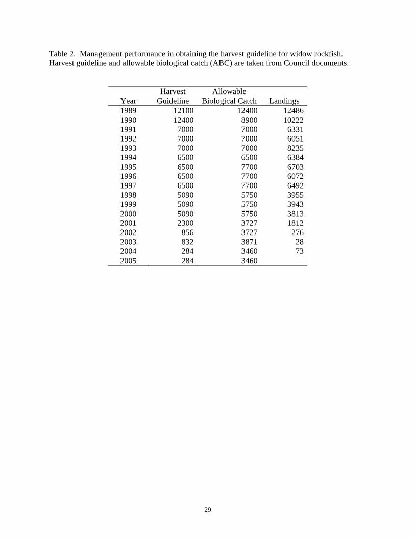
Year Harvest

Guideline Allowable

Biological Catch Landings 1989 12100 12400 12486 1990 12400 8900 10222 1991 7000 7000 6331 1992 7000 7000 6051 1993 7000 7000 8235 1994 6500 6500 6384 1995 6500 7700 6703 1996 6500 7700 6072 1997 6500 7700 6492 1998 5090 5750 3955 1999 5090 5750 3943 2000 5090 5750 3813 2001 2300 3727 1812 2002 856 3727 276 2003 832 3871 28 2004 284 3460 73 2005 284 3460

8

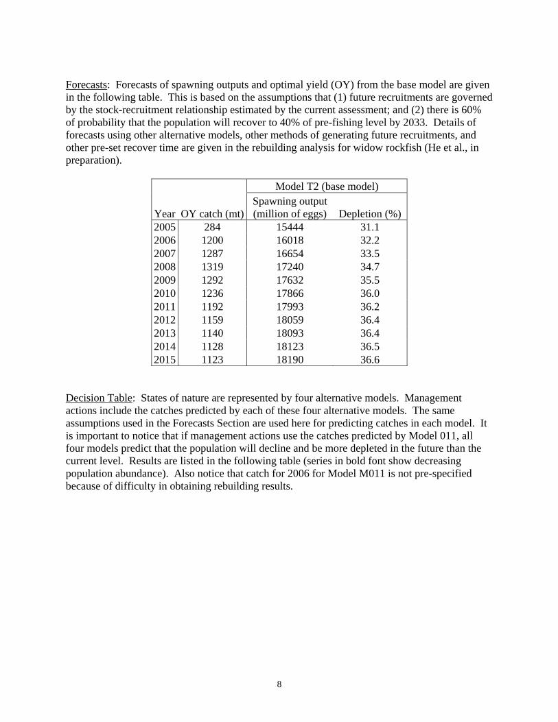
Forecasts: Forecasts of spawning outputs and optimal yield (OY) from the base model are given in the following table. This is based on the assumptions that (1) future recruitments are governed by the stock-recruitment relationship estimated by the current assessment; and (2) there is 60% of probability that the population will recover to 40% of pre-fishing level by 2033. Details of forecasts using other alternative models, other methods of generating future recruitments, and other pre-set recover time are given in the rebuilding analysis for widow rockfish (He et al., in preparation).

Model T2 (base model)

Year OY catch (mt)Spawning output (million of eggs) Depletion (%)

2005 284 15444 31.1 2006 1200 16018 32.2 2007 1287 16654 33.5 2008 1319 17240 34.7 2009 1292 17632 35.5 2010 1236 17866 36.0 2011 1192 17993 36.2 2012 1159 18059 36.4 2013 1140 18093 36.4 2014 1128 18123 36.5 2015 1123 18190 36.6

Decision Table: States of nature are represented by four alternative models. Management actions include the catches predicted by each of these four alternative models. The same assumptions used in the Forecasts Section are used here for predicting catches in each model. It is important to notice that if management actions use the catches predicted by Model 011, all four models predict that the population will decline and be more depleted in the future than the current level. Results are listed in the following table (series in bold font show decreasing population abundance). Also notice that catch for 2006 for Model M011 is not pre-specified because of difficulty in obtaining rebuilding results.

9

State of Nature Model T1 Model M015 Model T2 (base) Model M011 Management

action Year Total catch

(mt) Spawning

output Depletion

(%) Spawning

output Depletion

(%) Spawning

output Depletion

(%) Spawning

output Depletion

(%) 2005 285 8992 25.3 12052 25.8 15444 31.1 20351 38.5 2006 289 9746 27.4 12546 26.8 16018 32.2 21030 39.8 2007 2277 10655 30.0 13234 28.3 16839 33.9 21149 40.0 2008 2312 11092 31.2 13477 28.8 17230 34.7 21625 40.9 2009 2298 11361 31.9 13524 28.9 17407 35.0 21910 41.4 Model T1 2010 2275 11527 32.4 13408 28.7 17421 35.1 22058 41.7 2011 2262 11648 32.8 13195 28.2 17328 34.9 22135 41.9 2012 2272 11754 33.0 12933 27.7 17185 34.6 22166 41.9 2013 2302 11880 33.4 12697 27.2 17016 34.3 22139 41.9 2014 2333 12030 33.8 12465 26.7 16847 33.9 22111 41.8 2015 2376 12214 34.3 12292 26.3 16720 33.7 22088 41.8 2005 285 8992 25.3 12052 25.8 15444 31.1 20351 38.5 2006 289 9746 27.4 12546 26.8 16018 32.2 21030 39.8 2007 538 10655 30.0 13234 28.3 16839 33.9 21149 40.0 2008 556 11459 32.2 13832 29.6 17590 35.4 21989 41.6 2009 556 12113 34.1 14248 30.5 18150 36.5 22665 42.9 Model M015 2010 544 12663 35.6 14493 31.0 18548 37.3 23213 43.9 2011 533 13153 37.0 14618 31.3 18824 37.9 23683 44.8 2012 524 13604 38.3 14668 31.4 19035 38.3 24093 45.6 2013 523 14058 39.5 14715 31.5 19182 38.6 24427 46.2 2014 523 14512 40.8 14751 31.6 19331 38.9 24751 46.8 2015 527 14997 42.2 14844 31.8 19512 39.3 25079 47.4 2005 285 8992 25.3 12052 25.8 15444 31.1 20351 38.5 2006 289 9746 27.4 12546 26.8 16016 32.2 21030 39.8 2007 1352 10655 30.0 13234 28.3 16839 33.9 21149 40.0 2008 1385 11287 31.7 13666 29.2 17421 35.1 21819 41.3 2009 1375 11759 33.1 13907 29.7 17801 35.8 22310 42.2 Model T2 2010 1343 12129 34.1 13982 29.9 18017 36.3 22670 42.9 (base) 2011 1311 12449 35.0 13950 29.8 18125 36.5 22955 43.4 2012 1287 12746 35.8 13864 29.7 18170 36.6 23190 43.9 2013 1282 13061 36.7 13788 29.5 18184 36.6 23363 44.2 2014 1277 13382 37.6 13718 29.3 18206 36.6 23530 44.5 2015 1283 13748 38.7 13700 29.3 18270 36.8 23717 44.9 2005 285 8992 25.3 12052 25.8 15444 31.1 20351 38.5 2006 4388 9746 27.4 12546 26.8 16018 32.2 21030 39.8 2007 4503 10655 30.0 13234 28.3 16839 33.9 21149 40.0 2008 4440 10624 29.9 13025 27.9 16771 33.8 21162 40.0 2009 4285 10425 29.3 12624 27.0 16483 33.2 20969 39.7 Model M011 2010 4109 10159 28.6 12101 25.9 16058 32.3 20665 39.1 2011 3964 9901 27.8 11538 24.7 15577 31.4 20330 38.4 2012 3869 9679 27.2 10988 23.5 15102 30.4 19996 37.8 2013 3823 9546 26.8 10515 22.5 14661 29.5 19664 37.2 2014 3764 9446 26.6 10083 21.6 14242 28.7 19351 36.6 2015 3729 9415 26.5 9735 20.8 13914 28.0 19080 36.1

10

Recommendations:

1. There are increasingly fewer reliable abundance indices for widow rockfish. Recent management measures have undermined the ability to continue fishery dependent time series of relative abundance from the Oregon bottom trawl fishery and Pacific whiting fishery since 1999. The constant flux of the management regime suggests that there is little likelihood that meaningful CPUE indices can be developed from these fisheries in the future. The triennial bottom trawl survey may be the only data that can provide abundance indices in the future. More analysis should be done to either calibrate or compare triennial survey results with those from the NWFSC Combined survey.

2. Long-term recruitment index is a key datum series in the stock assessment. Continuation of the midwater juvenile trawl survey and recent increases in sampling intensity and spatial coverage will improve estimation confidence and data quality. Comparison and possibly integration of the existing juvenile survey results with a recently initiated survey by the fishing industry (Vidar Wespestad, pers. comm.) could also broaden the spatial extent of this index. The ability to infer direct and indirect estimates of year class strengths from surveys and other sources, as well as to better understand the relationship between environmental conditions in the California Current System, should improve short-term forecasts of productivity, biomass levels and allowable catches from stock assessments.

3. Preliminary information from recent bycatch monitoring suggest that discards may have decreased substantially compared to the assumed 16% currently used. New discard data should be analysed and, if warranted, past discard estimates should be adjusted.

4. The utility of hydro-acoustic surveys on widow rockfish abundance should be evaluated in future assessments.

5. Sample sizes for existing age-collection programs (by fishery and survey) should be increased substantially.

6. The age-composition for the triennial survey should be determined by applying year-specific age-length keys to the survey length-frequencies, and included in future assessments as a basis for estimating survey selectivity.

11

Introduction

Widow rockfish (Sebastes entomelas) is an important commercial groundfish species belonging to the scorpionfish family (Scorpaenidae). It ranges from southeastern Alaska to northern Baja California, where it frequents rocky banks at depths of 25-370m (Eschemeyer et al. 1983, Wilkins 1986). In those habitats it feeds on small pelagic crustaceans and fishes, including especially Sergestes similis, myctophids, and euphausiids (Adams 1987). There is no evidence that separate genetic stocks of widow rockfish occur along the Pacific coast and the species has been treated as one stock with four separate fisheries (Hightower and Lenarz 1990; Rogers and Lenarz 1993; Ralston and Pearson 1997, Williams et al. 2002).

A midwater trawl fishery for widow rockfish developed rapidly in the late 1970s and increased rapidly in 1980-82 (Gunderson 1984, Fig. 1 and Table 1). Large concentrations of widow rockfish had evidently gone undetected because aggregations of this species form at night and disperse at dawn, an atypical pattern for rockfish. Since the fishery first developed, substantial landings of widow rockfish have been made in all three west-coast states.

Management of the fishery began in 1982 when 75,000 lbs trip limits were introduced in an effort to curb the rapid expansion of the fishery (Tables 2-3). These were reduced to 30,000 lbs in 1983 and the fishery was managed by alteration of trip limits within the fishing season. A 10,500 mt/yr Allowable Biological Catch (ABC) for widow rockfish was instituted in 1983 (Table 3), but no harvest guideline was established. This form of management continued with alterations in ABC and trip limits until 1989 when a 12,100 mt/yr harvest guideline was implemented (Tables 2-3). From 1994-1997 the harvest guideline was changed to 6,500 mt and then reduced to 5090 mt/yr for 1998 to 2000. Based on the 2000 stock assessment and the rebuilding analysis of 2001 and 2003, the harvest guidelines were further reduced to 2,300 mt for 2001, 856 mt for 2002, 832 mt for 2003, and 284 mt for 2004 and 2005 (He et al. 2003a, He et al. 2003b).

This assessment used an age-based population model similar to those used in previous assessments (Ralston and Pearson 1997, Williams et al. 2000, He et al. 2003b). The model structure and code were similar as in the 2003 assessment (He et al. 2003b). In addition to including the new data from 2003 to 2004, this assessment examined the following options:

• Depletion rate is computed in the same way as in the 2003 rebuilding analysis (He and Punt 2003);

• Triennial survey index is included as abundance index; • Power transformation of midwater juvenile survey index is estimated instead of using

a fixed value; • Sample sizes for age composition data are replaced by effective sample size

(McAllister and Ianelli 1997, Maunder, in preparation); • A prior probability for stock-recruitment steepness is included in the likelihood

functions (He et al. in review). Data Biological information

Growth in length for widow rockfish has been described using von Bertalanffy growth equations in two papers by Lenarz (1987) and Pearson and Hightower (1991). In their analyses

12

it was determined that females attain a larger size compared to males and fish from the northern part of the range tend to be larger at age compared to those in the south. For these reasons we chose to use the sex-specific and area-specific estimates for length-at-age. Furthermore, we chose to use the estimates listed in Pearson and Hightower (1991), shown below and in Figure 2, because they are from a more recent and comprehensive analysis of widow rockfish growth compared to the analysis by Lenarz (1987). In order to match the fisheries, we used the Columbia-Eureka INPFC area border (43o Lat.) to delineate north from south.

Parameter Females (north)

Males (north)

Females (south)

Males (south)

Linf (cm) 50.54 44.0 47.55 41.5 K 0.14 0.18 0.2 0.25 t0 -2.68 -2.81 -0.17 -0.28

Sex-specific weight-at-age estimates were computed using the length-at-age estimates

above with sex-specific length-weight regressions for widow rockfish developed by Barss and Echeverria (1987) (Figure 2). The length-weight regression equation is βαLW = , where W is the weight (g) and L is the length (cm). The sex-specific parameter values used in this assessment are listed below:

Parameter Females Males α 0.00545 0.01188 β 3.28781 3.06631

Estimates of maturity and fecundity of female widow rockfish were obtained from Barss

and Echeverria (1987) and Boehlert et al. (1982), respectively. Age-specific maturity estimates were taken directly from the literature instead of fitting a parametric model (Figure 3), while age-specific fecundity was computed using the weight-fecundity regression:

605.71 261830.7F W= − (1) where F is fecundity (number of eggs) and W is weight (g). The weight-fecundity regression applied to the southern weight-at-age estimates resulted in negative values for ages 3 and 4. The weight-fecundity regression developed by Boehlert et al. (1982) was based on fish captured from Oregon and apparently does not apply to widow rockfish in the south. The maturity estimates shown in Figure 3 indicate a substantial difference in maturity-at-age between the north and south, with the northern fish maturing at an older age. Lacking any other estimate of fecundity for the south, we applied the weight-fecundity regression from the north and modified the estimates for ages 3-5 to approximate an asymptote to 0 (Figure 3). Landings

All landings for the period 1966-2002 were summarized into four areas (fisheries): (1) Vancouver-Columbia (VC); (2) Oregon mid-water trawl (ORMWT); (3) Oregon bottom trawl (ORBTWL); and (4) Eureka, Monterey, and Conception (EMC). Landings statistics used in this assessment were derived from four sources. First, all commercial landings from 1981 were extracted from the PacFIN database. Second, the very small annual recreational take of widow rockfish was extracted from the Marine Recreational Fishing Statistics Survey (MRFSS)

13

database. Third, all landings from 1966 to 1972, and some landings from 1973 to 1976 were directly taken from a summary table in Rogers (2003), who recently compiled summaries of foreign catches in the period. Fourth, some landing from 1973 to 1976 and all landings from 1977 to 1979 were directly copied from the last assessment (Williams et al. 2000). Summarized landings by year are presented in Table 1 and Figure 1.

As in the last assessments of widow rockfish, the data were pooled over states into INPFC area blocks. These in turn were collapsed into northern and southern areas, representing the U.S. Vancouver and Columbia areas (VC, ORMWT, and ORBTWL) and the Eureka, Monterey, and Conception areas (EMC), respectively. The northern and southern areas are conveniently delineated by the 43o latitude line. Within the southern area, widow rockfish landings were further condensed by summing over gears (i.e., trawl, other commercial, and recreational), providing annual estimates of landings from the southern area fishery. In the northern area, however, landings were partitioned into three separate fisheries; the Oregon midwater trawl fishery, the Oregon bottom trawl fishery, and the remaining catch of widow rockfish, referred to as the Vancouver-Columbia fishery. Because identification of gear types in Oregon (midwater or bottom trawl) did not begin until 1983, all landings in the northern area prior to that time were assigned to the Vancouver-Columbia “trawl” fishery.

It should be noted that there are some small discrepancies in the landing statistics between those recently extracted from the PacFIN data and those used in the last assessment. Overall, these discrepancies are very small. Age composition data

Widow rockfish otolith samples collected coastwide since 1989 have been aged at the Santa Cruz (Tiburon) Laboratory using the break and burn aging method (Pearson and Hightower 1991). Prior to 1989, the ages of all Vancouver-Columbia fish were obtained by researchers in the State of Washington, who used surface readings. Prior to 1987, Oregon widow rockfish were aged by investigators in Oregon, who used the break and burn aging method. All California fish were aged by Santa Cruz Laboratory personnel using the break and burn aging technique.

Age validation of widow rockfish was conducted by marginal increment analysis (Lenarz 1987). Hyaline-zone formation, the measure of annual growth, appears to occur between December and April (Pearson 1996). For convenience all widow rockfish are assumed to be born on January 1. Variation in the timing of the hyaline-zone formation occurs between fish from Washington and California, which could affect age determination. Knowledge of the timing variation can be used to avoid mis-ageing and ultimately the variation in hyaline-zone formation is not likely to result in major age discrepancies (Pearson 1996).

Washington provided ageing data from samples collected during commercial market sampling. The data were then expanded using relative catches from US Vancouver and Columbia areas. Oregon provided raw sample data which were expanded using methods described in Sampson and Crone (1997). California age data was extracted and expanded from the CALCOM database (Pearson and Erwin 1997).

New otolith samples from the Eureka-Conception area from 1978 and 1979 were discovered last year. The samples were analyzed and included in this assessment. The complete sex specific age composition data and sample size information for the four fisheries are presented in Tables 4-8 and Figures 4-7.

14

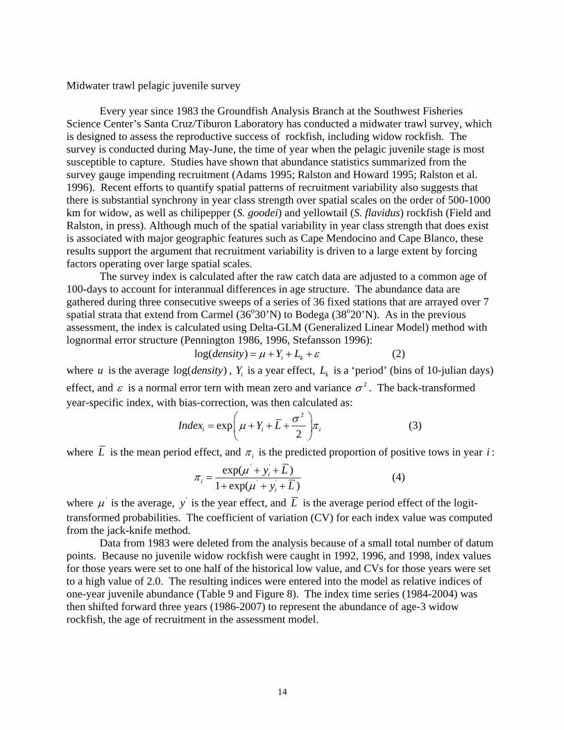
Midwater trawl pelagic juvenile survey

Every year since 1983 the Groundfish Analysis Branch at the Southwest Fisheries Science Center’s Santa Cruz/Tiburon Laboratory has conducted a midwater trawl survey, which is designed to assess the reproductive success of rockfish, including widow rockfish. The survey is conducted during May-June, the time of year when the pelagic juvenile stage is most susceptible to capture. Studies have shown that abundance statistics summarized from the survey gauge impending recruitment (Adams 1995; Ralston and Howard 1995; Ralston et al. 1996). Recent efforts to quantify spatial patterns of recruitment variability also suggests that there is substantial synchrony in year class strength over spatial scales on the order of 500-1000 km for widow, as well as chilipepper (S. goodei) and yellowtail (S. flavidus) rockfish (Field and Ralston, in press). Although much of the spatial variability in year class strength that does exist is associated with major geographic features such as Cape Mendocino and Cape Blanco, these results support the argument that recruitment variability is driven to a large extent by forcing factors operating over large spatial scales.

The survey index is calculated after the raw catch data are adjusted to a common age of 100-days to account for interannual differences in age structure. The abundance data are gathered during three consecutive sweeps of a series of 36 fixed stations that are arrayed over 7 spatial strata that extend from Carmel (36o30’N) to Bodega (38o20’N). As in the previous assessment, the index is calculated using Delta-GLM (Generalized Linear Model) method with lognormal error structure (Pennington 1986, 1996, Stefansson 1996):

log( ) i kdensity Y Lµ ε= + + + (2) where u is the average log( )density , iY is a year effect, kL is a ‘period’ (bins of 10-julian days) effect, and ε is a normal error tern with mean zero and variance 2σ . The back-transformed year-specific index, with bias-correction, was then calculated as:

2

exp2i i iIndex Y L σµ π

⎛ ⎞= + + +⎜ ⎟

⎝ ⎠ (3)

where L is the mean period effect, and iπ is the predicted proportion of positive tows in year i : ' ' '

' ' '

exp( )1 exp( )

ii

i

y Ly L

µπµ+ +

=+ + +

(4)

where 'µ is the average, 'y is the year effect, and 'L is the average period effect of the logit-transformed probabilities. The coefficient of variation (CV) for each index value was computed from the jack-knife method.

Data from 1983 were deleted from the analysis because of a small total number of datum points. Because no juvenile widow rockfish were caught in 1992, 1996, and 1998, index values for those years were set to one half of the historical low value, and CVs for those years were set to a high value of 2.0. The resulting indices were entered into the model as relative indices of one-year juvenile abundance (Table 9 and Figure 8). The index time series (1984-2004) was then shifted forward three years (1986-2007) to represent the abundance of age-3 widow rockfish, the age of recruitment in the assessment model.

15

Oregon bottom trawl logbook

Oregon logbook data from 1984 to 1986 were provided by the Oregon Department of Fish and Wildlife, and data from 1987 to 2002 were extracted from the PacFIN database. Catch per unit effort (CPUE) was computed as pounds of fish caught per hour trawled. The data were filtered before the analysis. Only records meeting the following criteria were used in the analysis: (1) the fishing gear code corresponded to bottom trawl or roller gear, (2) hauls were conducted during the months of January, February, or March, and (3) the location of the reported haul fell in the range of 42o30’N to 46o30’N latitude and 124o36’W to 124o54’W longitude. In addition, records associated with any vessel code or spatial unit that had less than 1000 pounds of widow catch over the entire period (1984 to 2002) were also deleted. Data from 2000 to 2002 were not used in the analysis because widow catches in those three years were very low due to trip limits and other management regulations (Tables 2 and 3).

Annual CPUE indices were derived using the Delta-GLM (Generalized Linear Model) method similar to that used for deriving midwater trawl pelagic juvenile survey (see previous section), with an additional factor (vessel) included:

log( ) i j k ijklCPUE Y V Lµ ε= + + + + (5) where u is the average log( )CPUE , iY is a year effect, jV is a vessel effect, kL is a spatial

(latitude and longitude) effect, and ijklε is a normal error tern with mean zero and variance 2εσ .

The back-transformed year-specific CPUE, with bias-correction, was then calculated as: 2

exp2i i iCPUE Y V L εσµ π

⎛ ⎞= + + + +⎜ ⎟

⎝ ⎠ (6)

where V and L are mean effects of vessel and spatial unit, respectively, and iπ is binomial coefficient:

' ' ' '

' ' ' '

exp( )1 exp( )

ii

i

y V Ly V L

µπµ+ + +

=+ + + +

(7)

where 'µ is the average, 'y is year effect, 'V is average vessel effect, and 'L is average spatial effect. Derived annual CPUE indices are presented in Table 10 and Figure 9, which are same as in the 2003 assessment. Pacific whiting bycatch indices

As in the previous assessments (Rogers and Lenarz 1993, Ralston and Pearson 1997, Williams et al. 2002), CPUE indices were computed that measured the incidental catch rate of widow rockfish in the at-sea pacific whiting fishery. Data from the foreign fishery, joint-venture fishery and recent domestic fishery were extracted from the NORPAC database.

Full descriptions on how the CPUE indices were derived are in Appendix A. Similar Delta-GLM approaches as used for the Oregon bottom trawl logbook is used in the analysis. Annual CPUE indices for the foreign fishery, joint-venture fishery, and domestic fisheries are presented in Table 11 and Figure 10. As recommended by the 2003 STAR Panel, annual CPUE indices from the domestic fishery after 1998 were excluded from the analysis because changes in management measures are expected to have more influence on the CPUE than changes in stock size. For this assessment, area-weighted CPUE indices were also computed, and comparisons of

16

the assessment results between the indices used in this assessment and the area-weighted indices are presented in Appendix A. Triennial trawl survey index The AFSC/NWFSC triennial trawl survey index was not used in the last assessment because of very limited widow catches by the survey and very poor fit of the index in the assessment model (He et al. 2003). The 2003 STAR panel recommended the index be analyzed further and be considered for inclusion in the assessment. Another important reason to include the triennial survey index in the assessment is that the index is likely going to be the only abundance index available in the future because other abundance indices from commercial fisheries will not be suitable for the assessment due to management regulations. The analysis of the triennial survey data uses the similar Delta-GLM method as for other indices, the results are presented in Table 12 and Figure 11, and detailed description of the analysis is in Appendix B. History of modeling approaches

Previous assessments for widow rockfish have been performed in 1989, 1990, 1993, 1997, 2000, and 2003 (Hightower and Lenarz 1989, 1990; Rogers and Lenarz 1993; Ralston and Pearson 1997, Williams et al 2000, He et al. 2003). In 1989 the assessment involved the use of cohort analysis and the stock synthesis program (Methot 1998). In 1993 and 1997, the age-based version of the stock synthesis program was used to assess the status of widow rockfish. In 2000 and 2003, the assessment of widow rockfish utilized AD Model Builder (ADMB) software (Otter Research, Ltd. 2001), and applied an age-based analysis of the population with methods very similar to those used in the stock synthesis program. The differences between the ADMB model and stock synthesis are minor. The ADMB model estimates landings with a very low coefficient of variation (0.05), while stock synthesis treats landings in a slightly different manner and the initial age composition estimation process is slightly different in the two models. A full description of the ADMB model follows and should clarify any further differences between this model and the stock synthesis program used in past assessments of widow rockfish. Model description General

This assessment uses an age-structured population model similar to the one used in the 2003 assessment (He et al. 2003). Full descriptions of the population dynamics, catch equations, and associated likelihood functions are given in Appendix C. The model is written in a C++ software language extension, AD Model Builder (ADMB) (Otter Research, Ltd. 2001), which utilizes automatic differentiation programming (Greiwank and Corliss 1991; Fournier 1996). The ADMB software allows for more rapid and accurate computation of derivative calculations used in the quasi-Newton optimization routine (Chong and Zak 1996). Further advantages of this software include the ability to estimate the variance-covariance matrix for all dependent and independent parameters of interest, likelihood profiling, and a Markov chain-Monte Carlo re-sampling algorithm for probability distribution determination.

17

The population model begins in 1958 and tracks numbers and catches of male and female widow rockfish in age classes 3-20 (age 20 is an age-plus group). In the 2000 assessment, a starting year of 1968 was chosen based on the assumption that the 1965 year class was the earliest recruitment which could be reasonably estimated given a starting year of 1980 for the age composition information. In the 2003 assessment and this assessment, the starting year was extended backward to 1958 because the new landing data from 1966 to 1972 were added. Recruitment estimates prior to 1958 are assumed equal to the 1958 estimate in the model, so that the model is estimating recruitment at age 3 for the years 1958-1999.

The data used in this model include 4 fishery catch-at-age compositions (sum across sexes equal to one), landings in weight for each fishery, NMFS Santa Cruz Laboratory midwater juvenile survey index, Oregon bottom trawl logbook CPUE, three whiting bycatch indices, and triennial survey indices. Predicted catch in each year is scaled to the fishery landings assuming a coefficient of variation of 5%. Double logistic selectivity functions by age were estimated for each fishery. Natural mortality

Natural mortality (M) is assumed to be constant for all ages and in all years. The initial model allowed the model to estimate a slightly higher natural mortality for males than females based on the observation that there were more old females than males in the age data. The model was presented to the 2003 STAR Panel. It was noted that greater proportions of males at younger ages could be due to differences in selectivity by gender. Allowing for different natural mortality had little impact on model results and the differences in M were small (<0.01). The 2003 STAR Panel considered that until the reason for the difference in age composition has been elucidated, the same natural mortality value should be used for both sexes. Therefore, natural mortality was fixed at 0.15 for the 2003 assessment. The 2005 STAR Panel requested that natural mortality be estimated in the model. After a series of model runs, it was decided natural mortality to be fixed at 0.125 for the base model, and two other values (0.11 and 0.15) to be used in alternative models to embrace uncertainties of model estimates.

Age compositions The age data are modeled as multinomial random variables, with the year-specific sample sizes set equal to the number of samples collected, rather than the number of fish, which often overstates the confidence of the data (Table 8) (Quinn and Deriso 1999). However, this assessment also examined an iterative-reweighting method to determine the effective sample size in the likelihood functions (details in the Likelihood component weighting section). Ageing error

The only information available for determination of ageing error was based on two point estimates of percent ageing agreement from the last two assessments (Rogers and Lenarz 1993; Ralston and Pearson 1997). From the previous assessments an estimate of 75% agreement for age 5 fish and 66% agreement for age 20 fish was modeled by assuming a linear relationship of percent agreement with age. These estimates of percent agreement at age were then fit to a set of

18

age-specific normal distributions, which approximated the level of ageing agreement. The resulting matrix of true age versus reader age was then placed in the model

t rA EA= (8) where tA and rA are n*n matrices for true age and reader age, respectively, n is number of age classes, and E is a n*n matrix for ageing error with the sum across each column equals to one. Landings

A constant CV of 0.05 is assumed for landing estimates. Year-specific fishing mortalities are computed for each fishery for those years in which there are landings estimates available. Fishing mortalities were zero from 1958 to 1965 since there are no landings estimates for those years. Fraction of landings in the north

Since there are area specific (north and south) estimates for weight-at-age and maturity, it is necessary to determine the fraction of the population to which each of these area-specific estimates apply. We used the sum of the domestic landings in the Vancouver-Columbia and both Oregon trawl fisheries relative to the total landings as an estimate of the proportion of the population to which the northern weight-at-age and maturity functions could be applied. Foreign landings from 1966 to 1976 from Rogers (2003) were not used in computing the fractions. The annual change in this fraction seemed highly variable and not likely to be indicative of true declines in area abundances. For this reason, the time series of proportions of landings in the north were smoothed using a 7-year moving average (Figure 12). The results from the moving average were then put directly into the model, applying the 1973 value to the earlier years. Discards

The level of discards of widow rockfish is virtually unknown in most of years. Age compositions in discards and landings can be very different (typically small fish are discarded) and can be important in determining discard rates (Williams et al. 1999). In past assessments a value of 6% of total weight was assumed for years 1958-1982 and 16% of total weight for the years 1983-2002 (Hightower and Lenarz 1990, Williams et al. 2000, He et al. 2003). The same discard rates (16%) were also applied for the years 2003-2004 in this assessment. The 16% estimate of discards is based on a dated study by Pikitch et al. (1988), which indicated most of the discards of widow rockfish were induced by regulations. The earlier 6% estimated is based on an ad hoc adjustment of the 16% by previous assessment authors (Hightower and Lenarz 1990). The 16% assumed value has likely become more uncertain in recent years due changes in regulations. For example, the most recent estimate on discard rate from the 2002 observer data, based on 89mt of widow rockfish catch, was 0.1%, which is much lower than the 16% assumed value. Midwater juvenile trawl survey

The Santa Cruz Laboratory midwater trawl juvenile survey is scaled to represent an index of 100 day-old larvae. For inclusion in the model the time series was lagged to correspond with

19

the appropriate year class. Within the model a catchability coefficient is estimated. In past assessments (Williams et al. 2002, He et al. 2003), a power coefficient was used for the midwater trawl survey. The power transformation was included to account for possible density dependent mortality occurring between 100 days of age and age 3 (the age of recruitment in the model), which likely results in higher variance levels in the survey time series relative to age 3 recruitment time series. However, the 2003 STAR panel argued that using power coefficient might dampen the estimate of recruitment variability. In this assessment, the power transformation is re-examined (see details in the Model Selection section). Test runs also showed that the results were only slightly different between using the power coefficient of 1.0 and 3.0, which was the default value in the 2003 assessment. Logbook and bycatch indices

The Oregon bottom trawl logbook indices and whiting bycatch indices are treated as biomass indices and are estimated in the model with a catchability parameter for each index. Because there were no new data since the 2003 assessment, the same Oregon bottom trawl logbook indices from the last assessment are used in this assessment. The whiting bycatch indices are recalculated according to the 2003 STAR panel recommendations, however the results are very similar. Details on the calculations of the whiting bycatch indices using Delta-GLM methods are in Appendix A. Calculation of depletion rate

Depletion rate is calculated as ratio of current spawning output over unfished spawning output. In the 2003 assessment, the depletion rate was calculated as ratio of the 2002 spawning output over the 1958 (first year in the model) spawning output. In this assessment, we calculate depletion rates using the same method as in the 2003 rebuilding analysis (He et al. 2003), which used the average of spawning outputs from 1958 to 1982 as unfished spawning output. This same calculation method will also be used for rebuilding analysis in 2005. Likelihood component weighting

There are nine likelihood components in the model (Appendix C): age-composition data, landings, recruitment residuals, midwater juvenile trawl survey index, four fisheries CPUE indices, and triennial survey indices. Weighting in this assessment model has two levels. First, contribution of each datum point to its likelihood component is weighted by a fixed CV associated with the datum point. Details on how a fixed CV is determined for each component are discussed later. Second, a weighting factors ( λ ) is assumed for each likelihood component and the final likelihood value for each component is multiplied by its weighting factor (Appendix C). In this assessment model, all weighting factor ( λ ) have been set to 1, except for the recruitment residual component and the midwater juvenile survey index component, whose weighting factors are 0.5.

For age composition data, this assessment examines an iterative-reweighting method to determine the effective sample size in the likelihood functions (McAllister and Ianelli 1997, Maunder, in preparation) for each year in each fishery. Initial sample size for each age composition data is taken directly from real sample sizes of the fishery. After the model is fitted

20

to the data, the observed and predicted proportions at age are used in the following equation to calculate effective sample size (T ):

( )

( )2

ˆ ˆ1

ˆ

a aa

a aa

p pT

p p

−=

−

∑∑

(9)

where ˆ ap is the predicted proportion and ap is the observed proportion at age a . The new sample size is then used in the model and the model is re-run. This process is repeated until the change in effective sample size is less than one percent between two consecutive runs. Because the sample size can differ substantially from year to year in a fishery, a linear regression of effective sample size versus observed sample size is used to obtain predicted effective sample size (MacCall 2003), which is then used in each iteration of the model run.

A prior for the steepness parameter in the stock-recruitment relations is also added in the likelihood functions (He at al. in review). The prior is based on a persistence principle that persistence of any species, given its life history and its exposure to recruitment variability, requires a minimum recruitment compensation that enables the species to rebound consistently from very low abundances. The prior curve for widow rockfish-like species has the following form:

h value

Pro

babi

lity

0.2 0.4 0.6 0.8 1.0

0.0

0.00

20.

004

0.00

6

A logistic equation that fits well with the curve is used in the likelihood function of the assessment model.

21

Model selection and evaluation

Initial model runs were performed using the same base model in the 2003 assessment (He et al. 2003), but with the new 2003 and 2004 data. After a series of sensitivity analysis and model examinations during the 2005 STAR Panel review, a final base model was selected (Model T2). It added new CPUE indices and used some new methods in the assessment model. These include:

• AFSC triennial bottom survey indices from 1977 to 2004 are included; • Depletion rate is computed in the same way as in the 2003 rebuilding analysis (He et al.

2003); • Power coefficient of midwater juvenile survey index is estimated instead of using a fixed

value; • An informative prior for recruitment steepness is included in the likelihood functions (He

et al., in review); • Sample sizes for age composition data are replaced by effective sample sizes.

Base model results

Results of the base model (Model T2) run are presented in Tables 13-14 and Figures 13-27. The resulting time series of total biomass, spawning biomass, spawning output, recruitment, and fishing mortality are presented in Table 13 and Figures 13-16. Estimated parameter values and their standard deviations are presented in Table 14. The fishery-specific selectivity curves are shown in Figure 17. The stock-recruitment relationship is shown in Figure 18. The fits to the landings are shown in Figures 19-20, and the fits to the various indices are shown in Figures 21-26. The fits of the age composition data are shown in Figure 27. Uncertainty and sensitivity analysis

Sensitivity analysis was done by comparing results between base model and three other models. Key features for four models are listed below:

Model name Recruitment steepness Natural mortality Selectivity Model T1 0.45 0.125 Double logistic / logisticModel M015 0.25 0.15 Double logistic Model T2 (base model) 0.28 0.125 Double logistic Model M011 0.32 0.11 Double logistic

These features were selected during the 2005 STAR Panel review to embrace uncertainties in model specifications and parameter estimates, especially for important parameter such as natural mortality. Biomass trends between the 2003 assessment base model and this assessment’s base model were compared (Figure 28). It is noted that the 2003 assessment estimated lower biomass between 1975 and 2002 than this assessment, and that the 2003 assessment estimated continuous decline of biomass during recent years while this assessment estimated an increase of biomass from 2001 to 2002.

22

Table 15 and Figures 29-31 show results of comparisons between base model and three alternative models. Table 14 also shows comparisons of depletion rates using different computation methods between the 2003 assessment and this assessment. Model T1, which uses logistic selectivity for the Vancouver-Columbia and Eureka-Conception fisheries before 1983, had the least number of parameters. This model estimated that the population was most depleted (depletion = 25.28%), but with the highest recruitment steepness ( h =0.4515). This model also estimated the lowest overall biomass and recruitments (Table 14, Figures 29 and 30). Model M015, which assumes natural mortality of 0.15 as used in previous assessments, estimated similar depletion (25.78%) as Model T1, but with the lowest recruitment steepness ( h =0.2540). Model T2 (base model) has the same number of parameters as Model M015 and Model M011, and estimated intermediate depletion and recruitment steepness. Model M011, which assumes natural mortality of 0.11, estimated the population was least depleted (depletion = 38.49%), and with moderate high recruitment steepness ( h =0.3161). Recruitments in recent years were very similar among Model T1, Model T2, and Model M015 (Figure 30). Historical depletion rates for all models are presented in Figure 31. It shows that the population was never depleted below the overfished threshold (25%) in Model T1, Model M011, and Model M015, but the population was overfished between 2001 and 2003. The depletion rates estimated by Model T1 were 23.4%, 23.0%, and 23.8% for 2001, 2002, and 2003, respectively. Rebuilding parameters

Unfished spawning output (B0) was calculated as an average from the first year (1958) to 1982, which is the same period used in the 2003 rebuilding analysis (He et al. 2003). Other rebuilding parameters were calculated in the same way as in the 2003 assessment. A separate C++ program was written (embedded in the ADMB program) to produce a data file (“rebuild.dat”) that can be directly inputted into the rebuilding program written by Punt (2005). Status of the stock

The percentage ratio of spawning output in 2004 to B0 is the population status. The point estimate, from the base model run, for the population status in 2004 is 31.09% (Table 15). Given that the population was declared as an overfished stock in previous assessments (Williams 2000, He et al. 2003), and the population status is within the precautionary zone (>25% and <40%), rebuilding analysis is needed to determine harvest projections and target fishing mortalities. Management Recommendations

The stock has declined since fishing began in the later 1970’s. The 2003 assessment showed that the spawning output in 2002 was just below 25% of unfished spawning output. This assessment shows that the spawning output in 2004 was within the precautionary zone. Therefore, it is necessary to conduct rebuilding analysis to determine harvest levels and related risks of each harvest levels (He et al. 2003).

23

Future research

1. There are increasingly fewer reliable abundance indices for widow rockfish. Recent management measures have undermined the ability to continue fishery dependent time series of relative abundance from the Oregon bottom trawl fishery and Pacific whiting fishery since 1999. The constant flux of the management regime suggests that there is little likelihood that meaningful CPUE indices can be developed from these fisheries in the future. The triennial bottom trawl survey may be the only data that can provide abundance indices in the future. More analysis should be done to either calibrate or compare triennial survey results with those from the NWFSC Combined survey.

2. The long-term recruitment index is a key datum series in the stock assessment. Continuation of the midwater juvenile trawl survey and recent increases in sampling intensity and spatial coverage will improve estimation confidence and data quality. Comparison and possibly integration of the existing juvenile survey results with a recently initiated survey by the fishing industry (Vidar Wespestad, pers. comm.) could also broaden the spatial extent of this index. The ability to infer direct and indirect estimates of year class strengths from surveys and other sources, as well as to better understand the relationship between environmental conditions in the California Current System, should improve short-term forecasts of productivity, biomass levels and allowable catches from stock assessments.

3. Preliminary information from recent bycatch monitoring suggests that discards may have decreased substantially compared to the assumed 16% currently used. New discard data should be analysed and, if warranted, past discard estimates should be adjusted.

4. The utility of hydro-acoustic surveys on widow rockfish abundance should be evaluated in future assessments.

5. Sample sizes for existing age-collection programs (by fishery and survey) should be increased substantially.

6. The age-composition for the triennial survey should be determined by applying year-specific age-length keys to the survey length-frequencies, and included in future assessments as a basis for estimating survey selectivity.

Acknowledgements

We would like to thank Theresa Tsou of Washington Department of Fish and Wildlife for providing catch-at-age data for Washington fisheries, Mark Karnowski of Oregon Department of Fish and Wildlife for providing catch-at-age data for Oregon fisheries, William Daspit of the PSMFC for updating catch data, Mark Wilkins of NOAA Fisheries for providing triennial survey data, Martin Dorn of NOAA Fisheries for providing Pacific whiting catch data, and John DeVore of the PFMC for providing the recent regulatory history of widow rockfish. We would also like to acknowledge the members of the stock assessment review (STAR) panel, Andre Punt (Chair), Mark Maunder, Robert Mohn, Anthony Smith, Michael Schirripa, Susan Ashcraft, and Pete Leipzig for their constructive reviews and making the review meeting an effective process.

24

Literature Cited Adams, P.B. 1987. The diet of widow rockfish Sebastes entomelas in northern California, pp.

37-41. In: W.H. Lenarz and D.R. Gunderson (eds.), Widow rockfish, proceedings of a workshop, Tiburon, California, December 11-12, 1980. NOAA Tech. Rep. NMFS 48.

Adams, P.B., editor. 1995. Progress in rockfish recruitment studies. Southwest Fisheries

Science Center Administrative Report, Tiburon Laboratory, T-95-01. Barss, W.H. and T.W. Echeverria. 1987. Maturity of widow rockfish Sebastes entomelas from

the northeastern Pacific, 1977-82, pp. 13-18. In: W.H. Lenarz and D.R. Gunderson (eds.), Widow rockfish, proceedings of a workshop, Tiburon, California, December 11-12, 1980. NOAA Tech. Rep. NMFS 48.

Boehlert, G.W., W.H. Barss, and P.B. Lamberson. 1982. Fecundity of widow rockfish, Sebastes

entomelas, off the coast of Oregon. Fish. Bull. 80:881-884. Burnham, K.P. and D.R. Anderson. 1998. Model selection and inference a practical

information-theoretic approach. Springer-Verlag New York Inc., NY. Chong, E.K.P. and S.H. Zak. 1996. An introduction to optimization. John Wiley & Sons, Inc.,

New York. Dorn, M.W., M.W. Saunders, C.D. Wilson, M.A. Guttormsen, K. Cooke, R. Kieser, and M.E.

Wilkins. 1999. Status of the coastal Pacific hake/whiting stock in U.S. and Canada in 1998. In: Appendix to the status of the Pacific coast groundfish fishery through 1999 and recommended acceptable biological catches for 2000, stock assessment and fishery evaluation. Pacific Fishery Management Council, Portland, OR.

Eschmeyer, W.N., E.S. Herald, and H. Hammann. 1983. A field guide to Pacific coast fishes of

North America. Houghton Mifflin Company, Boston, 336p. Field, J.C. and S.V. Ralston. In press. Spatial variability in California current rockfish

recruitment events. Can. J. Fish. Aquat. Sci. Fournier, D. 1996. An introduction to AD Model Builder for use in nonlinear modeling and

statistics. Otter Research Ltd., Sidney, British Columbia, Canada. Greiwank, A. and G.F. Corliss, editors. 1991. Automatic differentiation of algorithms: theory,

implementation and application. Proceedings of the SIAM Workshop on the Automatic Differentiation of Algorithms, Soc. Indust. And Applied Mathematics, Philadelphia.

Gunderson, D.R. 1984. The great widow rockfish hunt of 1980-82. N. Am. J. Fish. Man. 4:465-

468.

25

He, X., A. Punt, A.D. MacCall, and S.V. Ralston. 2003a. Rebuilding analysis for widow rockfish in 2003. Status of the Pacific coast groundfish fishery through 2003, stock assessment anf fishery evaluation, Volume I. Pacific Fisheries Management Council, Augest 2003.

He, X., A. Punt, A.D. MacCall, and S. Ralston. In preparation. Rebuilding analysis for widow

rockfish in 2005. He, X., S.V. Ralston, A.D. MacCall, D.E. Pearson, and E.J. Dick. 2003b. Status of the widow

rockfish resource in 2003. Status of the Pacific coast groundfish fishery through 2003, stock assessment and fishery evaluation, Volume I. Pacific Fisheries Management Council, August 2003.

He, X., M. Mangel, and A.D. MacCall. In review. A prior for steepness based on a persistence

principle. Submitted to Fishery Bulletin. Hightower, J.E. and W.H. Lenarz. 1990. Status of the widow rockfish stock in 1990. In: Status

of the Pacific coast groundfish fishery through 1990 and recommended biological catches for 1991 (Appendix F, Volume 2). Pacific Fishery Management Council, Portland, OR.

Lenarz, W.H. 1987. Ageing and growth of widow rockfish, pp. 31-35. In: W.H. Lenarz and

D.R. Gunderson (eds.), Widow rockfish, proceedings of a workshop, Tiburon, California, December 11-12, 1980. NOAA Tech. Rep. NMFS 48.

MacCall, A.D., S. Ralston, D. Pearson, and E.H. Williams. 1999. Status of bocaccio off

California in 1999 and outlook for the next millennium. In: Appendix to the status of the Pacific coast groundfish fishery through 1999 and recommended acceptable biological catches for 2000, stock assessment and fishery evaluation. Pacific Fishery Management Council, Portland, OR.

MacCall, A.D. 2003. Status of bocaccio off California in 2003. Status of the Pacific coast

groundfish through 2003, stock assessment and fishery evaluation, Volume I. Pacific Fisheries Management Council, August 2003.

Maunder, M.N. in preparation. Determing the effective sample size for over-dispersed

multinomial data: Appliation to catch-at-age data used in stock assessment models. Inter-American Tropical Tuna Commission, La Jolla, California.

McAllister, M.K. and J.N. Ianelli. 1997. Bayesian stocak assessment using catch-at-age data

and the sampling-importance resampling algorithm.. Can. J. Fish. Aquat. Sci. 52:284-300. Methot, R.D. 1998. Technical description of the stock synthesis assessment program.

Unpublished manuscript. NOAA, NMFS, Northwest Fisheries Science Center, Seattle, Washington. 48 p.

26

Pearson, D.E. 1996. Timing of hyaline-zone formation as related to sex, location, and year of capture in otoliths of the widow rockfish, Sebastes entomelas. Fish. Bull. 94:190-197.

Pearson, D.E. and J.E. Hightower. 1991. Spatial and temporal variability in growth of widow

rockfish (Sebastes entomelas). NOAA Tech. Memo. NMFS, NOAA-TM-NMFS-SWFSC-167, 43 p.

Pearson, D.E. and B. Erwin. 1997. Documentation of California’s commercial market sampling

data entry and expansion programs. NOAA Tech. Memo. NMFS, NOAA-TM-NMFS-SWFSC-240, 62 p.

Pennington, M. 1986. Some statistical techniques for estimating abundance indices from trawl

surveys. Fishery Bulletin, 84:519-525. Pennington, M. 1996. Estimating the mean and variance from highly skewed marine data.

Fishery Bulletin, 94:498-505. Pikitch, E.K., D.L. Erickson, and J.R. Wallace. 1988. An evaluation of the effectiveness of trip

limits as a management tool. Northwest and Alaska Fisheries Center, NWAFC Processed Rep. 88-27.

Punt, A.E. 2005. SSC default rebuilding analysis. Technical specifications and user manual.

Version 2.8a, April 2005. University of Washington, Seattle, Washington. Otter Reaserach Ltd. 2001. AD Model Builder. Otter Research Ltd, Sydney B.C., Canada. Quinn, T.J., II and R.B. Deriso. 1999. Quantitative fish dynamics. Oxford University Press,

Inc., New York. Quirollo, L.F. 1987. Review of data on historical catches of widow rockfish in northern

California, pp. 7-8. In: W.H. Lenarz and D.R. Gunderson (eds.), Widow rockfish, proceedings of a workshop, Tiburon, California, December 11-12, 1980. NOAA Tech. Rep. NMFS 48.

Ralston, S. 1999. Trends in standardized catch rate of some rockfishes (Sebastes spp.) from the

California trawl logbook database. Southwest Fisheries Science Center, Administrative Report SC-99-01.

Ralston, S. and D.F. Howard. 1995. On the development of year-class strength and cohort

variability in two northern California rockfishes Fish. Bull. 93:710-720. Ralston, S., J.N. Ianelli, R.A. Miller, D.E. Pearson, D. Thomas, and M.E. Wilkins. 1996. Status

of bocaccio in the Conception/Monterey/Eureka INPFC areas in 1996 and recommendations for management in 1997. In: Status of the Pacific coast groundfish fishery through 1996 and recommended acceptable biological catches for 1997, Pacific Fishery Management Council, Portland, OR.

27

Ralston, S. and D. Pearson. 1997. Status of the widow rockfish stock in 1997. In: Status of the

Pacific coast groundfish fishery through 1997 and recommended acceptable biological catches for 1998. Pacific Fishery Management Council, Portland, OR.

Ralston, S., D.E. Pearson, and J.A. Reynolds. 1998. Status of the chilipepper rockfish stock in

1998. In: Appendix to the status of the Pacific coast groundfish fishery through 1998 and recommended acceptable biological catches for 1999, stock assessment and fishery evaluation. Pacific Fishery Management Council, Portland, OR.

Rogers, J.B. and W.H. Lenarz. 1993. Status of the widow rockfish stock in 1993. In: Status of

the Pacific coast groundfish fishery through 1993 and recommended acceptable biological catches for 1994. Pacific Fishery Management Council, Portland, OR.

Rogers, J.B. 2003. Species allocation of Sebastes and Sebastolobus sp. Caught by foreign

contries of Washington, Oregon, and California, U.S.A. in 1965-1976. NMFS, Northwest Science Center.

Sampson, D.B. and P.R. Crone, editors. 1997. Commercial fisheries data collection procedures

for U.S. Pacific coast groundfish. NOAA Tech. Memo. NMFS, NMFS-NWFSC-31, 189 p. STAR Panel Report. 2005. Widow rockfish. Submitted to the Pacific Fishery Management

Council, Portland, OR. August 2005. Stefansson, G. 1996. Analysis of groundfish survey abundance data: combining the GLM and

delta approaches. ICES Journal of Marine Sciences, 53:577-588. Wilkins, M.E. 1986. Development and evaluation of methodologies for assessing and

monitoring the abundance of widow rockfish, Sebastes entomelas. Fish. Bull. 84(2):287-310.

Williams, E.H., S. Ralston, A.D. MacCall, D. Woodbury, and D.E. Pearson. 1999. Stock

assessment of the canary rockfish resource in the waters off southern Oregon and California in 1999. In: Appendix to the status of the Pacific coast groundfish fishery through 1999 and recommended acceptable biological catches for 2000, stock assessment and fishery evaluation. Pacific Fishery Management Council, Portland, OR.

Williams, E.H., A.D. MacCall, S. Ralston, and D.E. Pearson. 2000. Status of the widow

rockfish resource in Y2K. In: Appendix to the status of the Pacific coast groundfish fishery through 2000 and recommended acceptable biological catches for 2001, stock assessment and fishery evaluation. Pacific Fishery Management Council, Portland, OR.

28

Table 1. U.S. total landings (mt) of widow rockfish by four fisheries from 1966 to 2004.

Year Vancouver, Columbia

Oregon Midwater Trawl

Oregon Bottom Trawl

Eureka, Monterey, and Conception Total

1966 3670 96 37661967 3900 249 41491968 1693 336 20291969 356 21 3771970 554 0 5541971 701 0 7011972 410 13 4231973 617 207 8241974 293 280 5731975 454 358 8121976 948 412 13601977 1318 883 22011978 605 502 11071979 966 2326 32921980 16190 5666 218561981 21779 5227 270071982 14802 11245 260471983 3222 1452 1488 4325 104871984 1450 3568 1334 3506 98581985 1537 3185 871 3570 91631986 2559 2977 1171 2800 95071987 3722 4985 1169 3035 129111988 3078 4102 1121 2183 104841989 3378 4871 1971 2266 124861990 2241 3235 2167 2579 102221991 1176 1846 1940 1369 63311992 946 1149 2624 1331 60511993 1747 1755 3386 1347 82351994 1074 1678 2382 1248 63841995 1087 1394 2278 1944 67031996 965 1464 2114 1529 60721997 1016 1523 2245 1707 64921998 563 758 1330 1304 39551999 525 1721 794 902 39432000 380 2276 16 1141 38132001 302 966 39 505 18122002 65 155 6 51 2762003 16 8 0 5 282004 30 12 2 28 73

29

Table 2. Management performance in obtaining the harvest guideline for widow rockfish. Harvest guideline and allowable biological catch (ABC) are taken from Council documents.

Year Harvest

Guideline Allowable

Biological Catch Landings 1989 12100 12400 12486 1990 12400 8900 10222 1991 7000 7000 6331 1992 7000 7000 6051 1993 7000 7000 8235 1994 6500 6500 6384 1995 6500 7700 6703 1996 6500 7700 6072 1997 6500 7700 6492 1998 5090 5750 3955 1999 5090 5750 3943 2000 5090 5750 3813 2001 2300 3727 1812 2002 856 3727 276 2003 832 3871 28 2004 284 3460 73 2005 284 3460

30

Table 3. Chronology of the regulatory history of widow rockfish by the Pacific Fishery Management Council.

Date Regulation 10/13/82 75,000 lb trip limit 1/30/83 30,000 lb trip limit 9/10/83 1,000 lb trip limit

1/1/84 50,000 lb trip limit once per week 5/6/84 40,000 lb trip limit once per week 8/1/84 closed fishery with 1,000 trip limit for incidental catch 9/9/84 closed fishery

1/10/85 30,000 lb trip limit once a week or 60,000 lb trip limit once per two weeks, unlimited trips of less than 3,000 lbs

4/28/85 dropped 60,000 lb biweekly option 7/21/85 3,000 lb trip limit, unlimited number of trips

1/1/86 30,000 lb trip limit, only one weekly landing greater than 3,000 lbs 9/28/86 3,000 lb trip limit, unlimited number of trips

1/1/87 30,000 lb trip limit, only one weekly landing greater than 3000 lbs 11/25/87 closed fishery

1/1/88 30,000 lb trip limit, only one weekly landing greater than 3000 lbs, unlimited number of trips less than 3,000 lbs

9/21/88 3,000 lb trip limit, unlimited number of trips 1/1/89 30,000 lb trip limit, only one weekly landing greater than 3,000 lbs

4/26/89 10,000 lb trip limit once per week 10/11/89 3,000 lb trip limit with unlimited number of trips

1/1/90 15,000 lb trip limit once per week or 25,000 lb trip limit once per two weeks with only one landing greater than 3,000 lbs each week

12/12/90 closed fishery 1/1/91 10,000 lb trip limit per week or 20,000 lb trip limit every two weeks with only one landing

greater than 3,000 lbs per week 9/25/91 3,000 lb trip limit with unlimited number of trips

1/1/92 30,000 lbs cumulative landings every 4 weeks 5/9/92 change from 3" mesh to 4.5" mesh in codend for roller gear north of Point Arena

8/12/92 3,000 lb trip limit with unlimited number of trips 12/2/92 30,000 lb cumulative trip limit per 4 weeks 12/1/93 3,000 lb trip limit with unlimited number of trips 1/1/94 30,000 lb cumulative limit per calender month

12/1/94 3,000 lb trip limit with unlimited number of trips 1/1/95 30,000 lb cumulative limit per calender month

4/14/95 45,000 lb cumulative limit per calender month 9/8/95 4.5" mesh applies to entire net and bottom trawl 1/1/96 70,000 lb cumulative limit per two months 9/1/96 50,000 lb cumulative limit per two months

11/1/96 25,000 lb cumulative limit per two months 1/1/97 70,000 lb cumulative limit per two months 5/1/97 60,000 lb cumulative limit per two months 1/1/98 limited entry: 25,000 lb cumulative per two month period, open access: 12,500 lb cumulative

per two month period 5/1/98 limited entry: 30,000 lb cumulative per two month period

31

Table 3 (continued). Chronology of the regulatory history of widow rockfish by the Pacific Fishery Management Council.

Date Regulation 7/1/98 open access: 3,000 lb cumulative per month

10/1/98 limited entry: 19,000 cumulative per month 1/1/99 limited entry: cumulative limits: phase 1 - 70,000 lbs per period, phase 2 - 16,000 lbs per

period, phase 3 - 30,000 lbs per period. Open access: 2,000 lbs per month 5/1/99 limited entry: decrease phase 2 and phase 3 limits to 11,000 lbs 7/2/99 open access: 8,000 lb cumulative limit per month

10/1/99 limited entry: vessels in Oregon and Washington using 30,000 lb cumulative monthly limit must have midwater trawl gear aboard or a state cumulative limit will be imposed

1/1/00 Widow rockfish classified as a shelf species for regulatory purposes, 30,000 lbs/2 months for limited entry trawl, 3,000 lbs/month for limited entry fixed gear and open access

1/1/01 20,000 lbs/2 months for months of Jan-Apr and Sep-Oct; otherwise 10,000 lbs/2 months for midwater limited entry. 1,000 lbs/months for small footrope limited entry. 3,000 lbs/month for fixed gear limited entry. Open access: north - 3,000 lbs/month, south - 3,000 lbs per month with some monthly closures in some areas.

7/1/01 North - limited entry midwater trawl limits: 1,000 lbs/month 10/1/01 closed fishery for all except midwater, which may land 2,000 lbs/month in north for October,

then 25,000 lbs/2 months. 1/1/02 North - limited entry trawl: closed through November to midwater trawl except for small

bycatch in whiting fishery, in November 13,000 lbs/2 month with no more than 2 trips, small footrope trawl1000 lbs/month through September, then closed Sept-Oct, then 500 lbs/month Nov-Dec. South - limited entry trawl: midwater closed year round except for a small bycatch in the whiting fishery, small footrope trawl 1,000 lbs/month through July, then closed

1/1/03 North - limited entry trawl: midwater trawl closed through November except for small amount of bycatch in whiting fishery, 12,000 lbs/2 months for Nov-Dec. small footrope trawl - 300 lbs/month Jan-Apr and Nov-Dec, 1000 lbs/month May-Oct. North - limited entry fixed gear: 200 lbs/month. North - open access gear: 200 lbs/month. South - limited entry trawl: same as north for midwater and small footrope trawl. South - limited entry fixed gear: closed Mar-Apr, then variable 100 lbs/2 months to 250 lbs/2 months. South - - open access gear: same as limited entry fixed gear.

1/1/04 North - limited entry trawl: midwater trawl closed through November except for small amount of bycatch in whiting fishery (500 lbs/month during primary whiting season; combined widow and yellowtail trip limit of 500 lbs/trip with trips of at least 10,000 lbs of whiting), 12,000 lbs/2 months for Nov-Dec. small footrope trawl - 300 lbs/month Jan-Apr and Nov-Dec, 1000 lbs/month May-Oct. North - limited entry fixed gear: 200 lbs/month. North - open access gear: 200 lbs/month. South - limited entry trawl: closed. South - limited entry fixed gear between 40E10’ and 34E27’ N lat.: 300 lbs/2 months Jan-Feb and Sep-Dec, closed Mar-Apr, 200 lbs/2 months May-Aug. South - limited entry fixed gear south of 34E27’ N lat.: closed Jan-Feb, 2,000 lbs/2 months Mar-Dec. South - - open access gear between 40E10’ and 34E27’ N lat.: same as limited entry fixed gear. South – open access gear south of 34E27’ N lat.: closed Jan-Feb, 500 lbs/2 months Mar-Dec.

32

Table 3 (continued). Chronology of the regulatory history of widow rockfish by the Pacific Fishery Management Council.

Date Regulation 1/1/05

(regs. for 2005 and

2006)

North - limited entry trawl: large and small footrope trawl- 300 lbs/2 months; midwater trawl- closed except for small amount of bycatch in whiting fishery (500 lbs/month during primary whiting season; combined widow and yellowtail trip limit of 500 lbs/trip with trips of at least 10,000 lbs of whiting); selective flatfish trawl - 300 lbs/month Jan-Apr and Nov-Dec, 1000 lbs/month May-Oct. North - limited entry fixed gear: 200 lbs/month. North - open access gear: 200 lbs/month. South - limited entry trawl: large footrope and midwater trawl- closed; small footrope trawl- 300 lbs/month. South - limited entry fixed gear between 40E10’ and 34E27’ N lat.: 300 lbs/2 months Jan-Feb and Sep-Dec, closed Mar-Apr, 200 lbs/2 months May-Aug. South - limited entry fixed gear south of 34E27’ N lat.: 2,000 lbs/2 months Jan-Feb and May-Dec, closed Mar-Apr. South - - open access gear between 40E10’ and 34E27’ N lat.: same as limited entry fixed gear. South – open access gear south of 34E27’ N lat.: 500 lbs/2 months Jan-Feb and May-Dec, closed Mar-Apr.

7/1/05 South - limited entry fixed gear south of 34E27’ N lat.: 3,000 lbs/2 months Jul-Dec. South – open access gear south of 34E27’ N lat.: 750 lbs/2 months Jul-Dec.

33

Table 4a. Propotional age composition of males for the Vancouver-Columbia fishery with the sum across sexes equal to 1. Data are from 1980 to 2004.

Year Age

3 4 5 6 7 8 9 10 11 12 13 14 15 16 17 18 19 20+ 1980 0.000 0.000 0.009 0.022 0.020 0.056 0.096 0.111 0.046 0.029 0.012 0.013 0.006 0.004 0.002 0.002 0.001 0.003 1981 0.000 0.007 0.024 0.064 0.046 0.024 0.048 0.088 0.068 0.047 0.026 0.017 0.012 0.005 0.004 0.003 0.003 0.009 1982 0.000 0.008 0.030 0.084 0.031 0.045 0.021 0.021 0.033 0.072 0.045 0.034 0.035 0.021 0.014 0.009 0.005 0.017 1983 0.000 0.008 0.154 0.113 0.028 0.017 0.014 0.013 0.014 0.018 0.020 0.015 0.015 0.009 0.006 0.007 0.006 0.020 1984 0.000 0.003 0.054 0.161 0.083 0.033 0.014 0.004 0.006 0.007 0.008 0.013 0.013 0.011 0.007 0.008 0.008 0.029 1985 0.000 0.008 0.075 0.080 0.125 0.066 0.022 0.009 0.004 0.006 0.005 0.006 0.005 0.003 0.006 0.005 0.003 0.028 1986 0.000 0.007 0.060 0.174 0.075 0.049 0.014 0.006 0.005 0.005 0.003 0.003 0.005 0.006 0.003 0.002 0.002 0.029 1987 0.000 0.006 0.024 0.120 0.194 0.046 0.013 0.009 0.003 0.004 0.006 0.004 0.003 0.004 0.004 0.002 0.002 0.011 1988 0.000 0.000 0.015 0.060 0.137 0.199 0.035 0.013 0.005 0.002 0.001 0.003 0.003 0.001 0.000 0.001 0.001 0.014 1989 0.000 0.003 0.018 0.093 0.095 0.157 0.087 0.009 0.004 0.001 0.000 0.001 0.000 0.001 0.000 0.000 0.002 0.008 1990 0.000 0.000 0.025 0.077 0.153 0.068 0.097 0.030 0.011 0.005 0.001 0.000 0.000 0.000 0.001 0.001 0.001 0.007 1991 0.000 0.001 0.010 0.062 0.114 0.107 0.074 0.044 0.050 0.010 0.004 0.003 0.002 0.001 0.004 0.001 0.001 0.018 1992 0.000 0.003 0.020 0.031 0.072 0.077 0.082 0.049 0.052 0.029 0.020 0.008 0.005 0.003 0.002 0.000 0.001 0.012 1993 0.000 0.000 0.016 0.058 0.051 0.063 0.057 0.035 0.029 0.031 0.023 0.020 0.012 0.007 0.005 0.004 0.002 0.013 1994 0.000 0.001 0.011 0.041 0.087 0.057 0.045 0.037 0.028 0.023 0.026 0.016 0.013 0.011 0.005 0.004 0.003 0.017 1995 0.001 0.010 0.031 0.056 0.096 0.100 0.064 0.029 0.031 0.019 0.015 0.024 0.010 0.007 0.006 0.007 0.002 0.012 1996 0.001 0.012 0.059 0.112 0.104 0.058 0.033 0.018 0.013 0.010 0.008 0.006 0.008 0.002 0.003 0.003 0.002 0.008 1997 0.000 0.003 0.037 0.149 0.129 0.050 0.015 0.010 0.006 0.007 0.007 0.008 0.001 0.003 0.003 0.001 0.001 0.004 1998 0.000 0.001 0.014 0.043 0.146 0.110 0.040 0.015 0.007 0.009 0.008 0.003 0.002 0.002 0.007 0.001 0.000 0.006 1999 0.000 0.002 0.011 0.041 0.081 0.107 0.082 0.041 0.023 0.010 0.010 0.009 0.005 0.005 0.004 0.005 0.002 0.005 2000 0.000 0.000 0.005 0.058 0.113 0.071 0.073 0.073 0.038 0.013 0.012 0.005 0.002 0.009 0.006 0.003 0.002 0.005 2001 0.000 0.000 0.004 0.051 0.126 0.084 0.062 0.054 0.037 0.039 0.033 0.008 0.017 0.006 0.006 0.006 0.002 0.006 2002 0.000 0.002 0.020 0.025 0.057 0.097 0.063 0.052 0.024 0.025 0.011 0.014 0.002 0.002 0.005 0.002 0.002 0.003 2003 0.000 0.003 0.060 0.080 0.084 0.060 0.017 0.003 0.000 0.000 0.000 0.003 0.000 0.000 0.000 0.000 0.000 0.000 2004 0.000 0.000 0.035 0.102 0.044 0.040 0.028 0.010 0.013 0.005 0.003 0.005 0.003 0.002 0.103 0.003 0.000 0.106

34

Table 4b. Propotional age composition of females for the Vancouver-Columbia fishery with the sum across sexes equal to 1. Data are from 1980 to 2004.

Year Age

3 4 5 6 7 8 9 10 11 12 13 14 15 16 17 18 19 20+ 1980 0.000 0.000 0.009 0.018 0.014 0.026 0.088 0.142 0.085 0.063 0.035 0.018 0.021 0.019 0.005 0.007 0.006 0.013 1981 0.000 0.007 0.017 0.047 0.044 0.020 0.020 0.062 0.078 0.071 0.037 0.028 0.019 0.010 0.005 0.006 0.005 0.027 1982 0.000 0.008 0.018 0.060 0.029 0.042 0.019 0.015 0.015 0.049 0.040 0.040 0.033 0.032 0.017 0.015 0.006 0.037 1983 0.000 0.006 0.153 0.114 0.040 0.021 0.009 0.014 0.013 0.016 0.029 0.023 0.022 0.013 0.010 0.007 0.005 0.028 1984 0.001 0.002 0.044 0.152 0.075 0.026 0.018 0.005 0.006 0.007 0.011 0.017 0.025 0.024 0.020 0.011 0.014 0.081 1985 0.000 0.008 0.071 0.081 0.117 0.058 0.028 0.009 0.007 0.005 0.008 0.005 0.012 0.010 0.011 0.007 0.008 0.099 1986 0.000 0.002 0.053 0.178 0.091 0.070 0.020 0.013 0.004 0.007 0.008 0.006 0.009 0.008 0.008 0.009 0.003 0.061 1987 0.000 0.004 0.014 0.095 0.224 0.057 0.037 0.026 0.009 0.007 0.004 0.002 0.007 0.008 0.005 0.008 0.004 0.035 1988 0.000 0.002 0.007 0.056 0.151 0.206 0.035 0.017 0.012 0.008 0.003 0.000 0.003 0.001 0.000 0.001 0.000 0.007 1989 0.000 0.003 0.007 0.076 0.093 0.184 0.104 0.009 0.010 0.006 0.001 0.001 0.001 0.002 0.000 0.001 0.004 0.020 1990 0.000 0.001 0.028 0.062 0.116 0.078 0.119 0.059 0.012 0.006 0.003 0.003 0.000 0.001 0.002 0.001 0.001 0.029 1991 0.000 0.000 0.004 0.054 0.084 0.099 0.066 0.057 0.054 0.011 0.009 0.005 0.004 0.002 0.001 0.003 0.002 0.040 1992 0.000 0.003 0.023 0.025 0.055 0.091 0.082 0.057 0.069 0.046 0.030 0.012 0.008 0.004 0.001 0.004 0.002 0.024 1993 0.000 0.001 0.008 0.059 0.038 0.068 0.070 0.054 0.050 0.085 0.048 0.030 0.015 0.009 0.003 0.005 0.002 0.029 1994 0.004 0.003 0.013 0.047 0.074 0.068 0.044 0.054 0.041 0.043 0.052 0.035 0.025 0.016 0.013 0.008 0.004 0.031 1995 0.001 0.009 0.032 0.050 0.078 0.082 0.055 0.037 0.023 0.027 0.017 0.021 0.010 0.007 0.011 0.005 0.002 0.014 1996 0.000 0.002 0.068 0.112 0.108 0.064 0.054 0.024 0.014 0.018 0.013 0.011 0.017 0.005 0.004 0.002 0.002 0.019 1997 0.000 0.001 0.029 0.167 0.142 0.053 0.033 0.024 0.017 0.018 0.017 0.010 0.007 0.011 0.005 0.002 0.003 0.029 1998 0.000 0.001 0.012 0.048 0.165 0.153 0.047 0.020 0.023 0.023 0.020 0.021 0.014 0.004 0.011 0.005 0.002 0.017 1999 0.000 0.001 0.012 0.046 0.067 0.127 0.105 0.053 0.033 0.023 0.015 0.013 0.014 0.009 0.006 0.011 0.005 0.018 2000 0.000 0.000 0.002 0.053 0.088 0.097 0.077 0.069 0.046 0.021 0.010 0.009 0.006 0.006 0.006 0.009 0.002 0.007 2001 0.000 0.000 0.002 0.025 0.053 0.090 0.057 0.014 0.031 0.025 0.048 0.035 0.017 0.019 0.004 0.006 0.008 0.023 2002 0.000 0.002 0.024 0.025 0.027 0.102 0.097 0.042 0.044 0.033 0.028 0.025 0.022 0.009 0.002 0.011 0.005 0.020 2003 0.003 0.013 0.101 0.054 0.047 0.057 0.040 0.010 0.027 0.007 0.007 0.007 0.003 0.003 0.000 0.000 0.003 0.003 2004 0.000 0.002 0.031 0.123 0.054 0.061 0.068 0.038 0.031 0.016 0.020 0.012 0.007 0.002 0.002 0.002 0.013 0.016

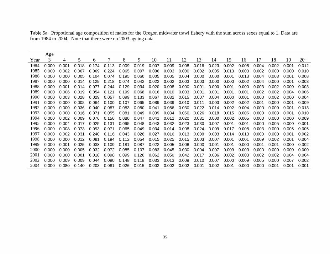
35

Table 5a. Propotional age composition of males for the Oregon midwater trawl fishery with the sum across sexes equal to 1. Data are from 1984 to 2004. Note that there were no 2003 ageing data.

Year Age

3 4 5 6 7 8 9 10 11 12 13 14 15 16 17 18 19 20+ 1984 0.000 0.001 0.018 0.174 0.113 0.009 0.019 0.007 0.009 0.008 0.016 0.023 0.002 0.008 0.004 0.002 0.001 0.012 1985 0.000 0.002 0.067 0.069 0.224 0.065 0.007 0.006 0.003 0.000 0.002 0.005 0.013 0.003 0.002 0.000 0.000 0.010 1986 0.000 0.000 0.005 0.104 0.074 0.195 0.060 0.005 0.005 0.004 0.000 0.000 0.001 0.013 0.004 0.003 0.001 0.008 1987 0.000 0.000 0.014 0.125 0.218 0.074 0.042 0.022 0.002 0.003 0.003 0.000 0.000 0.002 0.004 0.000 0.001 0.003 1988 0.000 0.001 0.014 0.077 0.244 0.129 0.034 0.020 0.008 0.000 0.001 0.000 0.001 0.000 0.003 0.002 0.000 0.003 1989 0.000 0.006 0.019 0.054 0.121 0.199 0.068 0.016 0.010 0.003 0.001 0.001 0.001 0.001 0.002 0.002 0.004 0.006 1990 0.000 0.003 0.028 0.029 0.057 0.099 0.133 0.067 0.032 0.015 0.007 0.004 0.000 0.001 0.000 0.002 0.000 0.004 1991 0.000 0.000 0.008 0.064 0.100 0.107 0.065 0.089 0.039 0.010 0.011 0.003 0.002 0.002 0.001 0.000 0.001 0.009 1992 0.000 0.000 0.036 0.040 0.087 0.083 0.080 0.041 0.086 0.030 0.022 0.014 0.002 0.004 0.000 0.000 0.001 0.013 1993 0.000 0.000 0.016 0.071 0.055 0.081 0.049 0.039 0.034 0.060 0.026 0.018 0.015 0.006 0.000 0.003 0.001 0.010 1994 0.000 0.002 0.009 0.076 0.156 0.080 0.047 0.041 0.012 0.020 0.031 0.000 0.002 0.005 0.000 0.000 0.000 0.009 1995 0.000 0.004 0.017 0.025 0.131 0.095 0.048 0.043 0.032 0.023 0.030 0.007 0.001 0.001 0.000 0.005 0.000 0.001 1996 0.000 0.008 0.073 0.093 0.071 0.065 0.049 0.034 0.014 0.008 0.024 0.009 0.017 0.008 0.003 0.000 0.005 0.005 1997 0.000 0.002 0.031 0.240 0.116 0.043 0.026 0.027 0.016 0.013 0.009 0.003 0.014 0.013 0.000 0.000 0.001 0.002 1998 0.000 0.000 0.012 0.081 0.194 0.112 0.054 0.015 0.025 0.015 0.003 0.007 0.001 0.001 0.009 0.002 0.001 0.004 1999 0.000 0.001 0.025 0.038 0.109 0.181 0.087 0.022 0.005 0.006 0.000 0.001 0.001 0.000 0.001 0.001 0.000 0.002 2000 0.000 0.000 0.005 0.032 0.072 0.085 0.107 0.083 0.045 0.030 0.004 0.007 0.009 0.003 0.000 0.000 0.000 0.000 2001 0.000 0.000 0.001 0.018 0.098 0.099 0.120 0.062 0.050 0.042 0.017 0.006 0.002 0.003 0.002 0.002 0.004 0.004 2002 0.000 0.009 0.009 0.044 0.090 0.148 0.118 0.033 0.013 0.009 0.010 0.007 0.000 0.009 0.005 0.000 0.007 0.002 2004 0.000 0.080 0.140 0.203 0.081 0.026 0.015 0.002 0.002 0.002 0.001 0.002 0.001 0.000 0.000 0.001 0.001 0.001

36

Table 5b. Propotional age composition of females for the Oregon midwater trawl fishery with the sum across sexes equal to 1. Data are from 1984 to 2004. Note that there were no 2003 ageing data.

Year Age

3 4 5 6 7 8 9 10 11 12 13 14 15 16 17 18 19 20+ 1984 0.000 0.002 0.020 0.162 0.181 0.015 0.030 0.006 0.007 0.004 0.028 0.061 0.016 0.009 0.007 0.006 0.006 0.018 1985 0.000 0.000 0.053 0.067 0.252 0.086 0.011 0.011 0.009 0.000 0.001 0.007 0.017 0.002 0.001 0.001 0.002 0.005 1986 0.000 0.000 0.010 0.137 0.082 0.168 0.067 0.004 0.011 0.004 0.000 0.000 0.004 0.016 0.001 0.002 0.002 0.009 1987 0.000 0.001 0.017 0.113 0.198 0.080 0.038 0.020 0.002 0.005 0.002 0.000 0.001 0.002 0.003 0.001 0.000 0.002 1988 0.001 0.005 0.015 0.077 0.192 0.099 0.026 0.017 0.009 0.004 0.004 0.000 0.001 0.000 0.001 0.004 0.003 0.004 1989 0.000 0.004 0.026 0.036 0.079 0.197 0.086 0.024 0.011 0.006 0.004 0.002 0.000 0.001 0.001 0.002 0.001 0.007 1990 0.000 0.000 0.018 0.034 0.054 0.079 0.151 0.104 0.037 0.022 0.009 0.002 0.002 0.001 0.001 0.000 0.000 0.004 1991 0.000 0.000 0.010 0.062 0.096 0.061 0.069 0.098 0.043 0.014 0.010 0.004 0.003 0.001 0.000 0.000 0.002 0.015 1992 0.000 0.000 0.023 0.030 0.070 0.075 0.042 0.064 0.089 0.031 0.015 0.006 0.001 0.002 0.002 0.002 0.000 0.008 1993 0.000 0.001 0.010 0.068 0.036 0.080 0.065 0.036 0.046 0.067 0.034 0.024 0.020 0.010 0.004 0.005 0.002 0.007 1994 0.000 0.000 0.008 0.049 0.158 0.064 0.056 0.041 0.035 0.025 0.029 0.015 0.021 0.005 0.000 0.000 0.002 0.003 1995 0.000 0.005 0.005 0.031 0.059 0.088 0.089 0.057 0.043 0.039 0.032 0.046 0.013 0.007 0.014 0.001 0.000 0.009 1996 0.000 0.007 0.067 0.059 0.077 0.080 0.049 0.024 0.039 0.016 0.018 0.023 0.018 0.006 0.001 0.001 0.001 0.027 1997 0.000 0.003 0.012 0.170 0.082 0.038 0.038 0.017 0.014 0.012 0.013 0.013 0.007 0.017 0.001 0.002 0.000 0.005 1998 0.000 0.000 0.004 0.037 0.158 0.092 0.048 0.031 0.032 0.015 0.015 0.012 0.004 0.002 0.007 0.001 0.003 0.005 1999 0.000 0.000 0.023 0.036 0.081 0.186 0.093 0.041 0.020 0.008 0.011 0.007 0.001 0.007 0.004 0.001 0.000 0.001 2000 0.000 0.000 0.009 0.031 0.071 0.098 0.079 0.091 0.060 0.027 0.016 0.007 0.009 0.004 0.003 0.001 0.006 0.005 2001 0.000 0.000 0.000 0.013 0.067 0.067 0.071 0.069 0.049 0.060 0.016 0.010 0.008 0.008 0.014 0.008 0.006 0.004 2002 0.000 0.003 0.009 0.018 0.065 0.114 0.091 0.082 0.036 0.033 0.015 0.005 0.009 0.000 0.005 0.000 0.002 0.002 2004 0.005 0.111 0.075 0.152 0.071 0.023 0.006 0.001 0.001 0.001 0.000 0.000 0.000 0.000 0.000 0.000 0.000 0.000

37

Table 6a. Propotional age composition of males for the Oregon bottom trawl fishery with the sum across sexes equal to 1. Data are from 1984 to 1999.

Year Age

3 4 5 6 7 8 9 10 11 12 13 14 15 16 17 18 19 20+ 1984 0.000 0.002 0.034 0.158 0.115 0.018 0.017 0.004 0.004 0.002 0.021 0.015 0.011 0.009 0.007 0.003 0.001 0.010 1985 0.000 0.003 0.049 0.097 0.195 0.049 0.003 0.005 0.002 0.000 0.001 0.004 0.026 0.000 0.007 0.001 0.000 0.007 1986 0.000 0.002 0.014 0.200 0.081 0.085 0.058 0.003 0.018 0.005 0.002 0.000 0.001 0.018 0.002 0.001 0.003 0.016 1987 0.000 0.000 0.011 0.111 0.204 0.072 0.040 0.016 0.003 0.002 0.007 0.000 0.000 0.006 0.005 0.002 0.000 0.008 1988 0.002 0.011 0.017 0.080 0.208 0.102 0.022 0.011 0.007 0.003 0.000 0.000 0.001 0.000 0.002 0.004 0.001 0.006 1989 0.000 0.009 0.025 0.051 0.094 0.176 0.064 0.027 0.014 0.008 0.000 0.005 0.000 0.000 0.001 0.001 0.006 0.007 1990 0.000 0.004 0.047 0.045 0.056 0.068 0.116 0.058 0.021 0.020 0.010 0.004 0.001 0.003 0.000 0.000 0.000 0.012 1991 0.000 0.000 0.004 0.066 0.100 0.072 0.042 0.078 0.037 0.010 0.012 0.003 0.001 0.004 0.000 0.000 0.001 0.011 1992 0.000 0.000 0.017 0.022 0.084 0.073 0.059 0.034 0.048 0.018 0.029 0.016 0.004 0.004 0.006 0.002 0.003 0.017 1993 0.000 0.000 0.006 0.035 0.035 0.088 0.091 0.047 0.033 0.054 0.035 0.023 0.014 0.004 0.002 0.004 0.000 0.017 1994 0.000 0.003 0.014 0.057 0.107 0.069 0.042 0.017 0.021 0.029 0.024 0.008 0.006 0.005 0.009 0.002 0.000 0.011 1995 0.000 0.003 0.034 0.109 0.074 0.135 0.039 0.044 0.021 0.018 0.007 0.012 0.005 0.005 0.005 0.000 0.000 0.002 1996 0.000 0.002 0.079 0.082 0.059 0.058 0.022 0.017 0.017 0.020 0.016 0.002 0.017 0.005 0.002 0.011 0.001 0.007 1997 0.000 0.006 0.044 0.230 0.118 0.047 0.031 0.021 0.009 0.018 0.007 0.006 0.001 0.006 0.002 0.000 0.000 0.004 1998 0.000 0.000 0.008 0.051 0.183 0.116 0.035 0.022 0.017 0.020 0.006 0.009 0.000 0.002 0.007 0.000 0.003 0.008 1999 0.000 0.004 0.028 0.066 0.118 0.177 0.072 0.027 0.009 0.000 0.000 0.007 0.001 0.000 0.000 0.000 0.007 0.003

38

Table 6b. Propotional age composition of females for the Oregon bottom trawl fishery with the sum across sexes equal to 1. Data are from 1984 to 1999.

Year Age

3 4 5 6 7 8 9 10 11 12 13 14 15 16 17 18 19 20+ 1984 0.000 0.000 0.033 0.135 0.188 0.031 0.018 0.013 0.008 0.005 0.014 0.034 0.017 0.009 0.005 0.006 0.003 0.049 1985 0.001 0.000 0.023 0.062 0.199 0.121 0.016 0.007 0.007 0.000 0.001 0.026 0.038 0.006 0.006 0.004 0.004 0.030 1986 0.000 0.001 0.025 0.106 0.062 0.096 0.068 0.007 0.018 0.013 0.000 0.000 0.004 0.044 0.010 0.007 0.005 0.025 1987 0.000 0.002 0.010 0.119 0.167 0.060 0.051 0.030 0.004 0.004 0.002 0.003 0.000 0.005 0.017 0.014 0.003 0.023 1988 0.010 0.014 0.009 0.077 0.172 0.103 0.041 0.027 0.015 0.010 0.005 0.006 0.001 0.002 0.006 0.010 0.003 0.010 1989 0.000 0.001 0.027 0.028 0.068 0.146 0.090 0.038 0.041 0.016 0.006 0.004 0.004 0.004 0.006 0.004 0.010 0.018 1990 0.000 0.000 0.046 0.036 0.037 0.068 0.137 0.107 0.036 0.017 0.009 0.005 0.007 0.002 0.002 0.001 0.001 0.024 1991 0.000 0.000 0.007 0.055 0.060 0.065 0.074 0.109 0.058 0.034 0.034 0.007 0.005 0.005 0.002 0.001 0.003 0.037 1992 0.000 0.000 0.010 0.008 0.082 0.089 0.069 0.058 0.090 0.048 0.032 0.020 0.014 0.005 0.006 0.001 0.003 0.031 1993 0.000 0.000 0.000 0.025 0.025 0.076 0.073 0.044 0.040 0.066 0.043 0.029 0.017 0.021 0.006 0.009 0.006 0.032 1994 0.000 0.002 0.009 0.043 0.100 0.063 0.057 0.063 0.046 0.026 0.065 0.029 0.020 0.012 0.012 0.007 0.006 0.016 1995 0.000 0.005 0.013 0.037 0.109 0.084 0.051 0.039 0.045 0.026 0.017 0.025 0.004 0.002 0.013 0.002 0.000 0.015 1996 0.000 0.007 0.076 0.102 0.082 0.086 0.051 0.028 0.041 0.032 0.008 0.004 0.040 0.000 0.002 0.010 0.003 0.011 1997 0.000 0.008 0.031 0.104 0.094 0.030 0.047 0.031 0.019 0.015 0.008 0.013 0.010 0.016 0.005 0.001 0.005 0.014 1998 0.000 0.000 0.012 0.047 0.141 0.110 0.054 0.024 0.030 0.017 0.026 0.013 0.016 0.003 0.008 0.002 0.001 0.009 1999 0.000 0.000 0.023 0.058 0.068 0.147 0.063 0.042 0.039 0.009 0.012 0.006 0.008 0.002 0.000 0.001 0.001 0.001

39

Table 7a. Propotional age composition of males for the Eureka-Conception fishery with the sum across sexes equal to 1. Data are from 1978 to 2004.

Year Age

3 4 5 6 7 8 9 10 11 12 13 14 15 16 17 18 19 20+ 1978 0.000 0.000 0.000 0.000 0.039 0.062 0.114 0.039 0.047 0.016 0.016 0.000 0.016 0.039 0.000 0.023 0.000 0.055 1979 0.000 0.000 0.000 0.000 0.011 0.012 0.049 0.017 0.020 0.016 0.009 0.017 0.002 0.019 0.011 0.020 0.000 0.048 1980 0.000 0.000 0.002 0.014 0.003 0.007 0.040 0.032 0.051 0.031 0.025 0.029 0.010 0.053 0.004 0.016 0.005 0.060 1981 0.001 0.008 0.010 0.027 0.025 0.028 0.026 0.030 0.043 0.047 0.024 0.033 0.016 0.029 0.012 0.004 0.014 0.025 1982 0.000 0.000 0.044 0.007 0.037 0.033 0.030 0.014 0.043 0.076 0.036 0.030 0.020 0.014 0.017 0.010 0.008 0.032 1983 0.000 0.000 0.023 0.140 0.032 0.033 0.013 0.005 0.008 0.009 0.020 0.020 0.012 0.012 0.005 0.023 0.002 0.027 1984 0.000 0.000 0.022 0.137 0.145 0.028 0.036 0.014 0.014 0.002 0.010 0.030 0.014 0.004 0.005 0.004 0.004 0.030 1985 0.000 0.000 0.009 0.062 0.163 0.145 0.013 0.025 0.011 0.002 0.003 0.010 0.022 0.002 0.005 0.003 0.003 0.027 1986 0.000 0.003 0.042 0.046 0.082 0.124 0.129 0.014 0.022 0.017 0.001 0.001 0.008 0.029 0.006 0.009 0.004 0.038 1987 0.001 0.000 0.055 0.114 0.044 0.060 0.091 0.112 0.020 0.030 0.021 0.003 0.000 0.019 0.015 0.003 0.011 0.026 1988 0.000 0.035 0.000 0.066 0.061 0.090 0.061 0.051 0.034 0.014 0.009 0.008 0.003 0.004 0.006 0.016 0.002 0.016 1989 0.000 0.005 0.109 0.073 0.078 0.119 0.046 0.050 0.020 0.012 0.020 0.016 0.008 0.000 0.000 0.007 0.006 0.009 1990 0.000 0.000 0.045 0.116 0.029 0.047 0.038 0.056 0.030 0.025 0.016 0.023 0.019 0.014 0.004 0.002 0.008 0.006 1991 0.000 0.002 0.015 0.119 0.120 0.049 0.038 0.065 0.022 0.016 0.020 0.012 0.002 0.004 0.004 0.003 0.003 0.017 1992 0.000 0.001 0.011 0.019 0.138 0.095 0.038 0.017 0.044 0.028 0.021 0.019 0.011 0.005 0.016 0.001 0.002 0.023 1993 0.000 0.000 0.085 0.163 0.096 0.078 0.010 0.002 0.009 0.007 0.011 0.001 0.021 0.005 0.002 0.004 0.001 0.033 1994 0.002 0.004 0.007 0.070 0.148 0.110 0.065 0.021 0.024 0.007 0.008 0.005 0.006 0.009 0.001 0.005 0.000 0.005 1995 0.000 0.033 0.039 0.034 0.056 0.197 0.045 0.066 0.058 0.003 0.028 0.007 0.021 0.001 0.004 0.008 0.000 0.003 1996 0.004 0.006 0.046 0.045 0.067 0.114 0.118 0.033 0.027 0.018 0.015 0.003 0.025 0.007 0.002 0.002 0.009 0.013 1997 0.000 0.002 0.008 0.108 0.041 0.051 0.052 0.048 0.050 0.036 0.027 0.023 0.013 0.005 0.004 0.012 0.006 0.012 1998 0.000 0.008 0.082 0.061 0.093 0.069 0.054 0.021 0.045 0.025 0.018 0.018 0.005 0.007 0.009 0.000 0.000 0.013 1999 0.001 0.001 0.019 0.072 0.059 0.101 0.069 0.051 0.027 0.022 0.030 0.016 0.006 0.006 0.006 0.012 0.005 0.031 2000 0.000 0.000 0.004 0.044 0.061 0.116 0.055 0.044 0.027 0.028 0.009 0.000 0.003 0.003 0.008 0.002 0.002 0.002 2001 0.000 0.000 0.000 0.010 0.073 0.012 0.064 0.092 0.035 0.040 0.032 0.030 0.042 0.021 0.004 0.003 0.000 0.007 2002 0.000 0.010 0.002 0.002 0.015 0.035 0.044 0.104 0.029 0.021 0.098 0.032 0.061 0.002 0.030 0.000 0.033 0.036 2003 0.000 0.279 0.013 0.009 0.009 0.035 0.040 0.040 0.000 0.018 0.000 0.004 0.013 0.013 0.000 0.000 0.000 0.004 2004 0.000 0.000 0.023 0.000 0.015 0.031 0.054 0.070 0.039 0.015 0.047 0.023 0.007 0.032 0.039 0.000 0.007 0.007

40

Table 7b. Propotional age composition of females for the Eureka-Conception fishery with the sum across sexes equal to 1. Data are from 1978 to 2004.

Year Age

3 4 5 6 7 8 9 10 11 12 13 14 15 16 17 18 19 20+ 1978 0.000 0.000 0.000 0.000 0.124 0.206 0.041 0.041 0.018 0.000 0.062 0.000 0.000 0.000 0.000 0.000 0.000 0.042 1979 0.000 0.000 0.000 0.000 0.029 0.067 0.158 0.062 0.061 0.040 0.075 0.011 0.019 0.036 0.011 0.023 0.030 0.127 1980 0.000 0.000 0.001 0.006 0.004 0.024 0.063 0.098 0.097 0.039 0.051 0.062 0.018 0.013 0.029 0.040 0.007 0.066 1981 0.000 0.003 0.005 0.014 0.036 0.019 0.025 0.055 0.073 0.091 0.027 0.056 0.046 0.039 0.025 0.040 0.011 0.035 1982 0.000 0.000 0.032 0.009 0.035 0.031 0.024 0.008 0.036 0.102 0.051 0.036 0.034 0.032 0.023 0.025 0.017 0.052 1983 0.000 0.010 0.075 0.167 0.047 0.048 0.015 0.009 0.002 0.008 0.037 0.022 0.012 0.028 0.020 0.016 0.026 0.071 1984 0.000 0.000 0.025 0.124 0.113 0.027 0.029 0.012 0.007 0.003 0.020 0.045 0.010 0.011 0.007 0.007 0.010 0.050 1985 0.000 0.000 0.002 0.039 0.153 0.144 0.020 0.039 0.006 0.002 0.003 0.010 0.023 0.002 0.006 0.007 0.009 0.031 1986 0.000 0.001 0.032 0.027 0.073 0.082 0.100 0.007 0.021 0.009 0.005 0.002 0.002 0.028 0.003 0.004 0.004 0.026 1987 0.001 0.000 0.047 0.095 0.021 0.051 0.051 0.055 0.011 0.010 0.004 0.002 0.001 0.004 0.003 0.006 0.001 0.011 1988 0.000 0.086 0.037 0.076 0.072 0.055 0.033 0.037 0.021 0.004 0.014 0.020 0.004 0.007 0.004 0.006 0.009 0.039 1989 0.000 0.003 0.082 0.043 0.042 0.081 0.054 0.038 0.021 0.010 0.008 0.004 0.006 0.006 0.000 0.001 0.001 0.022 1990 0.000 0.003 0.051 0.109 0.056 0.037 0.089 0.071 0.037 0.024 0.010 0.008 0.006 0.001 0.003 0.001 0.002 0.012 1991 0.000 0.007 0.008 0.113 0.128 0.061 0.030 0.033 0.023 0.017 0.013 0.011 0.008 0.008 0.007 0.001 0.002 0.018 1992 0.000 0.000 0.015 0.031 0.108 0.086 0.039 0.030 0.037 0.026 0.026 0.044 0.015 0.000 0.001 0.001 0.006 0.042 1993 0.000 0.004 0.033 0.135 0.124 0.097 0.037 0.004 0.001 0.010 0.008 0.001 0.001 0.001 0.001 0.005 0.005 0.007 1994 0.002 0.002 0.022 0.067 0.161 0.066 0.051 0.020 0.026 0.017 0.015 0.007 0.009 0.008 0.006 0.000 0.002 0.023 1995 0.000 0.008 0.009 0.015 0.050 0.137 0.050 0.068 0.023 0.005 0.008 0.002 0.005 0.008 0.000 0.008 0.000 0.001 1996 0.005 0.007 0.040 0.043 0.042 0.081 0.058 0.050 0.038 0.030 0.011 0.010 0.012 0.003 0.001 0.007 0.005 0.004 1997 0.000 0.001 0.007 0.083 0.038 0.056 0.053 0.042 0.065 0.048 0.030 0.020 0.005 0.021 0.006 0.007 0.005 0.014 1998 0.000 0.002 0.054 0.029 0.076 0.030 0.046 0.045 0.053 0.060 0.028 0.008 0.010 0.006 0.007 0.002 0.003 0.013 1999 0.000 0.002 0.010 0.074 0.046 0.094 0.042 0.047 0.038 0.022 0.021 0.015 0.014 0.014 0.004 0.009 0.002 0.013 2000 0.000 0.000 0.007 0.033 0.099 0.073 0.075 0.057 0.039 0.027 0.059 0.033 0.033 0.021 0.002 0.001 0.024 0.007 2001 0.000 0.000 0.000 0.008 0.060 0.099 0.037 0.065 0.064 0.032 0.038 0.023 0.021 0.001 0.013 0.023 0.034 0.018 2002 0.000 0.010 0.002 0.001 0.031 0.015 0.038 0.112 0.049 0.074 0.004 0.034 0.031 0.033 0.004 0.003 0.000 0.008 2003 0.013 0.412 0.040 0.000 0.000 0.013 0.004 0.022 0.004 0.000 0.000 0.013 0.000 0.000 0.000 0.000 0.000 0.000 2004 0.000 0.000 0.015 0.016 0.015 0.016 0.038 0.038 0.068 0.060 0.067 0.076 0.015 0.053 0.046 0.031 0.007 0.030

41

Table 8. Number of samples collected for each year and fishery of age composition data used in the widow rockfish assessment. Vancouver-

Columbia Oregon midwater

trawl Oregon bottom trawl Eureka-Conception

1978 7 1979 11 1980 18 26 1981 31 44 1982 40 149 1983 25 189 1984 22 32 27 169 1985 16 53 23 175 1986 27 56 22 154 1987 36 68 34 135 1988 20 39 33 127 1989 30 65 45 170 1990 41 61 49 155 1991 35 59 78 95 1992 31 43 82 55 1993 34 50 61 22 1994 28 22 63 28 1995 33 30 43 11 1996 25 32 27 35 1997 29 47 40 61 1998 22 41 30 37 1999 29 62 26 31 2000 21 55 17 2001 10 39 7 2002 12 17 14 2003 5 3 2004 19 4 7

42

Table 9. Yearly index estimates from the Santa Cruz/Tiburon Laboratory midwater trawl pelagic juvenile survey from 1984 to 2004.

Year Index value CV 1984 4.456 0.415206 1985 14.319 0.457595 1986 0.153 0.434277 1987 4.810 0.203188 1988 3.758 0.259248 1989 0.206 0.381102 1990 0.230 0.392817 1991 1.452 0.296396 1992 0.068 0.443453 1993 0.879 0.246520 1994 0.135 0.443453 1995 0.230 0.450612 1996 0.068 0.443453 1997 0.283 0.372287 1998 0.068 0.443453 1999 0.297 0.456079 2000 0.288 0.309768 2001 1.311 0.244552 2002 6.561 0.293078 2003 1.742 0.262856 2004 2.379 0.266954

Table 10. Oregon bottom trawl logbook catch-per-unit-effort index from 1984 to 1999.

Year CPUE (lbs./hr.) CV 1984 331.47 0.21211985 100.88 0.18751986 227.08 0.29281987 169.08 0.27301988 93.97 0.28971989 164.10 0.17491990 78.49 0.13481991 73.59 0.12751992 83.16 0.11791993 53.58 0.13141994 100.34 0.11281995 109.96 0.13871996 94.81 0.13571997 97.23 0.15021998 56.56 0.17181999 84.46 0.1684

43

Table 11. Scaled indices of widow rockfish catches derived from bycatch in three sectors of the Pacific whiting fisheries. Note that index values after 1998 were not used in this assessment.

Year Index CV Foreign

1977 0.770 0.115 1978 1.205 0.112 1979 0.703 0.119 1980 1.993 0.131 1981 0.728 0.126 1982 0.243 0.247 1984 2.937 0.125 1985 0.407 0.107 1986 1.111 0.103 1987 0.390 0.088 1988 0.513 0.124

Joint venture 1983 2.889 0.120 1985 0.776 0.117 1986 0.823 0.081 1987 0.320 0.087 1988 0.659 0.077 1989 0.824 0.064 1990 0.710 0.074

Domestic 1991 1.264 0.125 1992 0.781 0.125 1993 0.801 0.104 1994 1.465 0.068 1995 0.455 0.106 1996 1.018 0.082 1997 0.886 0.077 1998 1.330 0.079

Table 12. Indices of widow rockfish catches derived from triennial surveys from 1977 to 2004. Detailed description of the analysis is in Appendix B.

Year Index CV 1977 0.506 0.247 1980 0.382 0.332 1983 0.565 0.289 1986 0.353 0.351 1989 0.390 0.477 1992 0.461 0.364 1995 0.305 0.317 1998 0.692 0.313 2001 0.112 0.350 2004 0.126 0.461

44

Table 13. Estimated age 3 recruits, age 3+ biomass, spawning biomass, spawning outputs, and annual fishing mortality of widow rockfish from 1958 to 2004 from the base model.

Year Age 3 Recruits

(103) Age 3+

Biomass (mt)Spawning

Biomass (mt) Spawning Output

(106 eggs) Fishing

Mortality 1958 34509 230505 112557 44904 0.000000 1959 34836 231687 112605 44905 0.000000 1960 35136 233164 112810 44922 0.000000 1961 35165 234823 113245 44996 0.000000 1962 33910 236270 113913 45167 0.000000 1963 32742 237373 114767 45437 0.000000 1964 29178 237410 115613 45759 0.000000 1965 31197 237529 116318 46084 0.000000 1966 23706 235548 116668 46351 0.036478 1967 37325 232387 114581 45676 0.041365 1968 39173 229946 111871 44742 0.020479 1969 40117 230756 110524 44156 0.003965 1970 41811 234416 110755 43994 0.005849 1971 44367 239082 111610 44041 0.007160 1972 40465 243147 113225 44391 0.004135 1973 89101 259807 115804 45063 0.007511 1974 32175 265099 118443 45834 0.004858 1975 12357 264142 122871 46972 0.006616 1976 10108 259304 127278 48587 0.010256 1977 16332 253355 129633 50425 0.015891 1978 21601 246373 129096 51385 0.008418 1979 10251 236002 125712 51001 0.026238 1980 38902 229729 119518 49122 0.227006 1981 57581 210808 102378 42491 0.366297 1982 20936 181547 83887 34716 0.447040 1983 66060 167675 68401 27663 0.243075 1984 77951 175342 64412 25243 0.227238 1985 28033 173484 63490 24085 0.195050 1986 28601 172748 64592 23757 0.179788 1987 28770 170056 66833 24357 0.206849 1988 22500 160241 66979 24756 0.159942 1989 9961 148981 66048 24891 0.205760 1990 24253 137885 61694 23704 0.182916

45

Table 13 (continued). Estimated age 3 recruits, age 3+ biomass, spawning biomass, spawning outputs, and annual fishing mortality of widow rockfish from 1958 to 2004 from the base model.

Year Age 3 Recruits

(103) Age 3+

Biomass (mt)Spawning

Biomass (mt) Spawning Output

(106 eggs) Fishing

Mortality 1991 15480 126761 57451 22427 0.121770 1992 15827 120069 54980 21659 0.125041 1993 29059 117532 52088 20622 0.191516 1994 43798 117761 47939 19016 0.163827 1995 13461 113199 45414 17847 0.183220 1996 15160 108431 43681 16805 0.169068 1997 12222 102959 43489 16474 0.163523 1998 6586 94966 43083 16406 0.095073 1999 7052 89754 42851 16566 0.104394 2000 9622 84787 41348 16306 0.112583 2001 25820 84098 39119 15663 0.058742 2002 23850 86603 37789 15241 0.009983 2003 17341 89936 37847 15137 0.000996 2004 17643 93685 39032 15337 0.002184

46

Table 14. Estimated parameter values and their standard deviations for the base model. Parameter description Estimated value Estimated standard deviation Mean recruitment 10.346000 0.110980Recruitment steepness 0.280960 0.056704Recruitment deviation in 1958 0.103250 0.866710Recruitment deviation in 1959 0.112690 0.866190Recruitment deviation in 1960 0.121250 0.863450Recruitment deviation in 1961 0.122070 0.856240Recruitment deviation in 1962 0.085718 0.842500Recruitment deviation in 1963 0.050438 0.816640Recruitment deviation in 1964 -0.065852 0.771830Recruitment deviation in 1965 -0.001385 0.652600Recruitment deviation in 1966 -0.279750 0.581210Recruitment deviation in 1967 0.169660 0.398980Recruitment deviation in 1968 0.213500 0.337660Recruitment deviation in 1969 0.233650 0.283720Recruitment deviation in 1970 0.284310 0.241720Recruitment deviation in 1971 0.356820 0.208490Recruitment deviation in 1972 0.273230 0.213420Recruitment deviation in 1973 1.064900 0.131150Recruitment deviation in 1974 0.045657 0.187050Recruitment deviation in 1975 -0.916390 0.245910Recruitment deviation in 1976 -1.126900 0.240130Recruitment deviation in 1977 -0.657920 0.185950Recruitment deviation in 1978 -0.393790 0.152700Recruitment deviation in 1979 -1.160300 0.190180Recruitment deviation in 1980 0.150440 0.107980Recruitment deviation in 1981 0.531070 0.094079Recruitment deviation in 1982 -0.476040 0.129460Recruitment deviation in 1983 0.696080 0.081536Recruitment deviation in 1984 0.953780 0.065616Recruitment deviation in 1985 0.067473 0.092484Recruitment deviation in 1986 0.251030 0.101160Recruitment deviation in 1987 0.325680 0.104770Recruitment deviation in 1988 0.115750 0.111920Recruitment deviation in 1989 -0.688500 0.143700Recruitment deviation in 1990 0.182170 0.108160Recruitment deviation in 1991 -0.279230 0.120010Recruitment deviation in 1992 -0.261240 0.124180Recruitment deviation in 1993 0.383810 0.113160Recruitment deviation in 1994 0.837030 0.113080Recruitment deviation in 1995 -0.315470 0.155040Recruitment deviation in 1996 -0.157750 0.154640Recruitment deviation in 1997 -0.308220 0.181380

47

Table 14 (continued). Estimated parameter values and their standard deviations for the base model. Parameter description Estimated value Estimated standard deviation Recruitment deviation in 1998 -0.874970 0.230550Recruitment deviation in 1999 -0.757190 0.264110Recruitment deviation in 2000 -0.429960 0.286380Recruitment deviation in 2001 0.560490 0.262490Recruitment deviation in 2002 0.473040 0.429260Recruitment deviation in 2003 0.167500 0.529180Recruitment deviation in 2004 0.218260 0.515420Selectivity parameter 1 for fishery 1 2.522700 0.141370Selectivity parameter 2 for fishery 1 5.869900 0.058679Selectivity parameter 3 for fishery 1 0.150240 0.013263Selectivity parameter 4 for fishery 1 0.000000 0.001278Selectivity parameter 1 for fishery 2 2.434400 0.151440Selectivity parameter 2 for fishery 2 6.227300 0.085509Selectivity parameter 3 for fishery 2 0.280000 0.030910Selectivity parameter 4 for fishery 2 7.590900 2.229600Selectivity parameter 1 for fishery 3 2.463900 0.186070Selectivity parameter 2 for fishery 3 6.022500 0.090360Selectivity parameter 3 for fishery 3 0.207510 0.041259Selectivity parameter 4 for fishery 3 9.944900 3.609100Selectivity parameter 1 for fishery 4 2.373300 0.285650Selectivity parameter 2 for fishery 4 5.669900 0.118340Selectivity parameter 3 for fishery 4 0.340740 0.093586Selectivity parameter 4 for fishery 4 17.116000 1.300600Average fishing mortality for fishery 1 -4.121100 0.120190Average fishing mortality for fishery 2 -3.466400 0.146620Average fishing mortality for fishery 3 -4.642600 0.157110Average fishing mortality for fishery 4 -4.960500 0.133350Deviation of fishing mortality for Fishery 1 in 1966 0.788240 0.154600Deviation of fishing mortality for Fishery 1 in 1967 0.883650 0.138880Deviation of fishing mortality for Fishery 1 in 1968 0.079480 0.123900Deviation of fishing mortality for Fishery 1 in 1969 -1.457000 0.115770Deviation of fishing mortality for Fishery 1 in 1970 -1.021900 0.105000Deviation of fishing mortality for Fishery 1 in 1971 -0.819320 0.096131Deviation of fishing mortality for Fishery 1 in 1972 -1.393900 0.089306Deviation of fishing mortality for Fishery 1 in 1973 -1.024500 0.084202Deviation of fishing mortality for Fishery 1 in 1974 -1.810100 0.081010Deviation of fishing mortality for Fishery 1 in 1975 -1.419700 0.079876Deviation of fishing mortality for Fishery 1 in 1976 -0.785150 0.079817Deviation of fishing mortality for Fishery 1 in 1977 -0.488240 0.083886Deviation of fishing mortality for Fishery 1 in 1978 -1.192400 0.088913

48

Table 14 (continued). Estimated parameter values and their standard deviations for the base model. Parameter description Estimated value Estimated standard deviation Deviation of fishing mortality for Fishery 1 in 1979 -0.604890 0.093628Deviation of fishing mortality for Fishery 1 in 1980 2.396100 0.094136Deviation of fishing mortality for Fishery 1 in 1981 2.947500 0.088638Deviation of fishing mortality for Fishery 1 in 1982 2.857400 0.078267Deviation of fishing mortality for Fishery 1 in 1983 1.544000 0.070693Deviation of fishing mortality for Fishery 1 in 1984 0.630710 0.067596Deviation of fishing mortality for Fishery 1 in 1985 0.645300 0.065048Deviation of fishing mortality for Fishery 1 in 1986 1.022300 0.062900Deviation of fishing mortality for Fishery 1 in 1987 1.225600 0.060763Deviation of fishing mortality for Fishery 1 in 1988 1.024100 0.058616Deviation of fishing mortality for Fishery 1 in 1989 1.204300 0.056619Deviation of fishing mortality for Fishery 1 in 1990 0.891590 0.056282Deviation of fishing mortality for Fishery 1 in 1991 0.328440 0.057213Deviation of fishing mortality for Fishery 1 in 1992 0.213960 0.058394Deviation of fishing mortality for Fishery 1 in 1993 0.920400 0.061520Deviation of fishing mortality for Fishery 1 in 1994 0.525880 0.066658Deviation of fishing mortality for Fishery 1 in 1995 0.618520 0.074207Deviation of fishing mortality for Fishery 1 in 1996 0.480600 0.084697Deviation of fishing mortality for Fishery 1 in 1997 0.425120 0.096282Deviation of fishing mortality for Fishery 1 in 1998 -0.174240 0.105520Deviation of fishing mortality for Fishery 1 in 1999 -0.183700 0.115370Deviation of fishing mortality for Fishery 1 in 2000 -0.423110 0.127470Deviation of fishing mortality for Fishery 1 in 2001 -0.546850 0.136790Deviation of fishing mortality for Fishery 1 in 2002 -2.004900 0.139150Deviation of fishing mortality for Fishery 1 in 2003 -3.427100 0.138720Deviation of fishing mortality for Fishery 1 in 2004 -2.876100 0.144510Deviation of fishing mortality for Fishery 2 in 1983 0.463790 0.100360Deviation of fishing mortality for Fishery 2 in 1984 1.188700 0.093829Deviation of fishing mortality for Fishery 2 in 1985 0.942000 0.089544Deviation of fishing mortality for Fishery 2 in 1986 0.755480 0.086006Deviation of fishing mortality for Fishery 2 in 1987 1.049400 0.081699Deviation of fishing mortality for Fishery 2 in 1988 0.764860 0.078017Deviation of fishing mortality for Fishery 2 in 1989 1.023600 0.072812Deviation of fishing mortality for Fishery 2 in 1990 0.732680 0.066586Deviation of fishing mortality for Fishery 2 in 1991 0.259910 0.062615Deviation of fishing mortality for Fishery 2 in 1992 -0.103890 0.060155Deviation of fishing mortality for Fishery 2 in 1993 0.454450 0.056682Deviation of fishing mortality for Fishery 2 in 1994 0.503960 0.053895Deviation of fishing mortality for Fishery 2 in 1995 0.417450 0.054159Deviation of fishing mortality for Fishery 2 in 1996 0.474370 0.058122

49

Table 14 (continued). Estimated parameter values and their standard deviations for the base model. Parameter description Estimated value Estimated standard deviation Deviation of fishing mortality for Fishery 2 in 1997 0.384400 0.066420Deviation of fishing mortality for Fishery 2 in 1998 -0.396970 0.076255Deviation of fishing mortality for Fishery 2 in 1999 0.479580 0.083790Deviation of fishing mortality for Fishery 2 in 2000 0.855620 0.094598Deviation of fishing mortality for Fishery 2 in 2001 0.110840 0.103240Deviation of fishing mortality for Fishery 2 in 2002 -1.615200 0.105160Deviation of fishing mortality for Fishery 2 in 2003 -4.576400 0.105030Deviation of fishing mortality for Fishery 2 in 2004 -4.168600 0.113130Deviation of fishing mortality for Fishery 3 in 1983 1.287800 0.099723Deviation of fishing mortality for Fishery 3 in 1984 1.087100 0.092506Deviation of fishing mortality for Fishery 3 in 1985 0.601150 0.087699Deviation of fishing mortality for Fishery 3 in 1986 0.788940 0.084355Deviation of fishing mortality for Fishery 3 in 1987 0.609310 0.080487Deviation of fishing mortality for Fishery 3 in 1988 0.519050 0.076711Deviation of fishing mortality for Fishery 3 in 1989 1.154300 0.071588Deviation of fishing mortality for Fishery 3 in 1990 1.340500 0.065599Deviation of fishing mortality for Fishery 3 in 1991 1.301800 0.061705Deviation of fishing mortality for Fishery 3 in 1992 1.696200 0.059167Deviation of fishing mortality for Fishery 3 in 1993 2.053200 0.055838Deviation of fishing mortality for Fishery 3 in 1994 1.792200 0.053282Deviation of fishing mortality for Fishery 3 in 1995 1.837000 0.053338Deviation of fishing mortality for Fishery 3 in 1996 1.771800 0.056995Deviation of fishing mortality for Fishery 3 in 1997 1.736700 0.064832Deviation of fishing mortality for Fishery 3 in 1998 1.176800 0.074658Deviation of fishing mortality for Fishery 3 in 1999 0.707960 0.082197Deviation of fishing mortality for Fishery 3 in 2000 -3.103100 0.092052Deviation of fishing mortality for Fishery 3 in 2001 -2.140900 0.100350Deviation of fishing mortality for Fishery 3 in 2002 -4.003600 0.102060Deviation of fishing mortality for Fishery 3 in 2003 -7.309700 0.101720Deviation of fishing mortality for Fishery 3 in 2004 -4.904500 0.108510Deviation of fishing mortality for Fishery 4 in 1966 -2.185100 0.141070Deviation of fishing mortality for Fishery 4 in 1967 -1.204200 0.129340Deviation of fishing mortality for Fishery 4 in 1968 -0.878960 0.117580Deviation of fishing mortality for Fishery 4 in 1969 -3.633600 0.110020Deviation of fishing mortality for Fishery 4 in 1970 -6.681500 0.101810Deviation of fishing mortality for Fishery 4 in 1971 -6.700500 0.094571Deviation of fishing mortality for Fishery 4 in 1972 -4.161900 0.088972Deviation of fishing mortality for Fishery 4 in 1973 -1.424900 0.084793Deviation of fishing mortality for Fishery 4 in 1974 -1.157500 0.082052Deviation of fishing mortality for Fishery 4 in 1975 -0.956770 0.080789

50

Table 14 (continued). Estimated parameter values and their standard deviations for the base model. Parameter description Estimated value Estimated standard deviation Deviation of fishing mortality for Fishery 4 in 1976 -0.897740 0.080601Deviation of fishing mortality for Fishery 4 in 1977 -0.166740 0.083639Deviation of fishing mortality for Fishery 4 in 1978 -0.696170 0.088076Deviation of fishing mortality for Fishery 4 in 1979 0.907870 0.092465Deviation of fishing mortality for Fishery 4 in 1980 1.941400 0.093744Deviation of fishing mortality for Fishery 4 in 1981 2.096600 0.089573Deviation of fishing mortality for Fishery 4 in 1982 3.155400 0.079800Deviation of fishing mortality for Fishery 4 in 1983 2.465700 0.072923Deviation of fishing mortality for Fishery 4 in 1984 2.237300 0.069269Deviation of fishing mortality for Fishery 4 in 1985 2.249000 0.065978Deviation of fishing mortality for Fishery 4 in 1986 1.903100 0.064633Deviation of fishing mortality for Fishery 4 in 1987 1.852100 0.063103Deviation of fishing mortality for Fishery 4 in 1988 1.501800 0.061701Deviation of fishing mortality for Fishery 4 in 1989 1.584600 0.059767Deviation of fishing mortality for Fishery 4 in 1990 1.779900 0.058793Deviation of fishing mortality for Fishery 4 in 1991 1.202300 0.059224Deviation of fishing mortality for Fishery 4 in 1992 1.241800 0.059778Deviation of fishing mortality for Fishery 4 in 1993 1.330700 0.062227Deviation of fishing mortality for Fishery 4 in 1994 1.343200 0.067397Deviation of fishing mortality for Fishery 4 in 1995 1.864400 0.074459Deviation of fishing mortality for Fishery 4 in 1996 1.636000 0.084537Deviation of fishing mortality for Fishery 4 in 1997 1.693800 0.096173Deviation of fishing mortality for Fishery 4 in 1998 1.426800 0.106910Deviation of fishing mortality for Fishery 4 in 1999 1.092100 0.116820Deviation of fishing mortality for Fishery 4 in 2000 1.386600 0.128640Deviation of fishing mortality for Fishery 4 in 2001 0.642700 0.137520Deviation of fishing mortality for Fishery 4 in 2002 -1.602100 0.139050Deviation of fishing mortality for Fishery 4 in 2003 -3.904700 0.137450Deviation of fishing mortality for Fishery 4 in 2004 -2.282800 0.139990Power coefficient for SC Lab index 0.145890 0.096683Catchbility for SC Lab index -10.201000 0.226500Catchbility for Oregon bottom trawl fishery -6.405300 0.176410Catchbility for whiting bycatch (foreign) -11.462000 0.233930Catchbility for whiting bycatch (joint venture) -11.247000 0.319280Catchbility for whiting bycatch (domestic) -10.785000 0.187220Catchbility for triennial trawl survey -12.194000 0.206290

51

Table 15. Comparisons between base model (Model T2) and other models.

Parameter and estimate Model T1 Model M015Model T2

(base model) Model M011Number of parameters 196 198 198 198 Steepness (h) 0.4515 0.2540 0.2810 0.3161 Unfished spawning output (B0) (million of eggs) 35564 46750 49676 52871 Current spawning output (Bt) (million of eggs) 8992 12051 15444 20350 Depletion (100*Bt/B0) 25.28 25.78 31.09 38.49 Standard deviation of depletion 5.61 4.96 5.92 6.95 Depletion calculated as in 2003 assessment 26.96 30.14 34.16 40.77

Figure 1. U.S. landings (mt) of widow rockfish by four fisheries from 1966 to 2002. Four fisheries are defined by area and gear type.

0

5000

10000

15000

20000

25000

30000

1966

1968

1970

1972

1974

1976

1978

1980

1982

1984

1986

1988

1990

1992

1994

1996

1998

2000

2002

2004

Lan

ding

s (m

t)

.

Vancouver-ColumbiaOregon Midwater TrawlOregon Bottom TrawlEureka-Conception

52

Figure 2. Growth functions for widow rockfish by sex from north and south of 43o latitude used in this assessment.

Age

Leng

th (c

m)

4 6 8 10 12 14 16 18 20

2530

3540

4550

Female (North)Male (North)Female (South)Male (South)

Age

Wei

ght (

kg)

4 6 8 10 12 14 16 18 20

0.2

0.6

1.0

1.4

1.8

Weight vs. age

Female (North)Male (North)Female (South)Male (South)

53

Figure 3. Fecundity and maturity for widow rockfish from north and south of 43o latitude used in this assessment.

Age

Milli

on o

f egg

s

4 6 8 10 12 14 16 18 20

0.0

0.2

0.4

0.6

0.8

NorthSouth

Age

Per

cent

mat

urity

(%)

4 6 8 10 12 14 16 18 20

010

2030

4050

6070

8090

NorthSouth

54

Figure 4. Proportional age composition data for the Vancouver-Columbia combined fishery, by sex and year with the sum across sexes equal to 1.

3 4 5 6 7 8 9 10 11 12 13 14 15 16 17 18 19 20+

1980

1981

1982

1983

198419851986198719881989199019911992199319941995199619971998199920002001200220032004

0.00

0.10

0.20

Prop

ortio

n

Age

Year

Males

3 4 5 6 7 8 9 10 11 12 13 14 15 16 17 18 19 20+

1980

1981

1982

1983

198419851986198719881989199019911992199319941995199619971998199920002001200220032004

0.00

0.20

0.40

Prop

ortio

n

Age

Year

Females

55

Figure 5. Proportional age composition data for the Oregon midwater trawl fishery, by sex and year with the sum across sexes equal to 1.

3 4 5 6 7 8 9 10 11 12 13 14 15 16 17 18 19 20+

1984

1985

1986

1987

1988

1989

1990

1991

1992199319941995199619971998199920002001200220032004

0.00

0.10

0.20

0.30

Prop

ortio

n

Age

Year

Males

3 4 5 6 7 8 9 10 11 12 13 14 15 16 17 18 19 20+

1984

1985

1986

1987

1988

1989

1990

1991

1992199319941995199619971998199920002001200220032004

0.00

0.10

0.20

0.30

Prop

ortio

n

Age

Year

Females

56

Figure 6. Proportional age composition data for the Oregon bottom trawl fishery, by sex and year with the sum across sexes equal to 1.

3 4 5 6 7 8 9 10 11 12 13 14 15 16 17 18 19 20+

1984

1985

1986

1987

1988

1989

1990

1991

1992

1993

1994

1995

1996

199719981999

0.00

0.10

0.20

0.30

Age

pr

opor

tion

Age

Year

Males

3 4 5 6 7 8 9 10 11 12 13 14 15 16 17 18 19 20+

1984

1985

1986

1987

1988

1989

1990

1991

1992

1993

1994

1995

1996

1997

19981999

0.00

0.10

0.20

Age

pr

opor

tion

Age

Year

Females

57

Figure 7. Proportional age composition data for the Eureka-Conception combined fishery, by sex and year with the sum across sexes equal to 1.

3 4 5 6 7 8 9 10 11 12 13 14 15 16 17 18 19 20+

1978

1979

1980198119821983198419851986198719881989199019911992199319941995199619971998199920002001200220032004

0.00

0.20

0.40

Prop

orti

on

Age

Year

Males

3 4 5 6 7 8 9 10 11 12 13 14 15 16 17 18 19 20+

1978

1979

1980

198119821983198419851986198719881989199019911992199319941995199619971998199920002001200220032004

0.00

0.50

Prop

orti

on

Age

Year

Females

58

Figure 8. Yearly index estimates from the Santa Cruz/Tiburon Laboratory midwater juvenile trawl survey from 1984 to 2004.

Year

Inde

x va

lue

1984 1988 1992 1996 2000 2004

02

46

810

1214

Figure 9. Catch per unit effort of widow rockfish from Oregon bottom trawl fishery from 1984 to 1999.

Year

CP

UE

(lbs

/hr)

1984 1986 1988 1990 1992 1994 1996 1998

5010

015

020

025

030

0

59

Figure 10. Scaled index values of catch per unit effort of widow rockfish abundance derived from bycatch in the Pacific whiting fisheries.

Year

Inde

x va

lue

1977 1979 1981 1983 1985 1987

0.5

1.5

2.5

Foreign

Year

Inde

x va

lue

1983 1984 1985 1986 1987 1988 1989 1990

0.5

1.5

2.5

Joint venture

Year

Inde

x va

lue

1991 1992 1993 1994 1995 1996 1997 1998

0.6

1.0

1.4 Domestic

60

Figure 11. Index values of catch per unit effort of widow rockfish abundance derived from triennial surveys.

Year

Inde

x va

lue

1980 1985 1990 1995 2000 2005

0.1

0.2

0.3

0.4

0.5

0.6

0.7

Triennial survey index

Figure 12. Fraction of landings in the north area, defined as the Vancouver-Columbia and Oregon trawl fisheries, with a 7-year moving average. Note that the fractions before 1977 were fixed at the value computed before the foreign landings (Rogers 2003) were added.

0.2

0.3

0.4

0.5

0.6

0.7

0.8

0.9

1

1965 1970 1975 1980 1985 1990 1995 2000 2005Year

Prop

ortio

n of

land

ings

in N

orth

.

61

Figure 13. Age 3+ biomass (1000mt) and spawning biomass (1000mt) from 1958 to 2004 estimates from the base model.

Year

Bio

mas

s (1

000m

t)

1958 1964 1970 1976 1982 1988 1994 2000

050

100

150

200

250

Age 3+ biomass and spawning biomass

Age 3+ biomassSpawning biomass

Figure 14. Spawning output (million of eggs) from 1958 to 2004 estimated from the base model.

Year

Spa

wni

ng o

utpu

t (m

illio

n of

egg

s)

1958 1964 1970 1976 1982 1988 1994 2000

010

000

2500

040

000

Spawning output (millions of eggs)

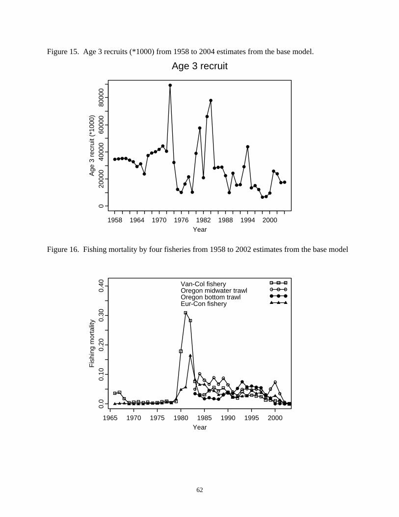
62

Figure 15. Age 3 recruits (*1000) from 1958 to 2004 estimates from the base model.

Year

Age

3 re

crui

t (*1

000)

1958 1964 1970 1976 1982 1988 1994 2000

020

000

4000

060

000

8000

0

Age 3 recruit

Figure 16. Fishing mortality by four fisheries from 1958 to 2002 estimates from the base model

Year

Fish

ing

mor

talit

y

1965 1970 1975 1980 1985 1990 1995 2000

0.0

0.10

0.20

0.30

0.40 Van-Col fishery

Oregon midwater trawlOregon bottom trawlEur-Con fishery

63

Figure 17. Fishery-specific selectivity estimates from the base model.

Age

Sel

ectiv

ity

4 6 8 10 12 14 16 18 20

0.0

0.2

0.4

0.6

0.8

1.0

Vancouver-Columbia fishery

Age

Sel

ectiv

ity

4 6 8 10 12 14 16 18 20

0.0

0.2

0.4

0.6

0.8

1.0

Oregon midwater trawl

Age

Sel

ectiv

ity

4 6 8 10 12 14 16 18 20

0.0

0.2

0.4

0.6

0.8

1.0

Oregon bottom trawwl

Age

Sel

ectiv

ity

4 6 8 10 12 14 16 18 20

0.0

0.2

0.4

0.6

0.8

1.0

Eureka-Conception fishery

64

Figure 18. Stock-recruitment relationship from the base model. Estimated +Residual = predicted values plus annual recruitment residuals; Estimated = estimated values from stock-recruitment relationship.

Spawning output (billion of eggs)

Rec

ruit

(*10

0000

0)

0 5 10 15 20 25 30 35 40 45 50

010

2030

4050

6070

8090 Estimated+residual

Estimated

65

Figure 19. Model fits to the Vancouver-Columbia and Oregon midwater trawl fisheries landings data.

Year

Land

ing

(100

0mt)

1966 1972 1978 1984 1990 1996 2002

02

46

810

1418

22

Vancouver-Columbia fishery

EstimatedObserved

Year

Land

ing

(100

0mt)

1984 1988 1992 1996 2000 2004

0.0

1.0

2.0

3.0

4.0

5.0

Oregon midwater trawl fishery

EstimatedObserved

66

Figure 20. Model fits to the Oregon bottom trawl and Eureka-Conception fisheries landings data.

Year

Land

ing

(100

0mt)

1984 1988 1992 1996 2000 2004

0.0

0.5

1.0

1.5

2.0

2.5

3.0

3.5

Oregon bottom trawl fishery

EstimatedObserved

Year

Land

ing

(100

0mt)

1966 1972 1978 1984 1990 1996 2002

02

46

810

Eureka-Conception fishery

EstimatedObserved

67

Figure 21. Model fits to the midwater trawl juvenile survey index.

Year

Inde

x va

lue

(pow

er tr

ansf

orm

ed)

1984 1986 1988 1990 1992 1994 1996 1998 2000

0.4

0.6

0.8

1.0

1.2

1.4

1.6

1.8

2.0

Midwater trawl juvenile survey

EstimatedObserved

Figure 22. Model fits to the Oregon bottom trawl logbook index.

Year

CP

UE

(lbs

/hr)

1984 1986 1988 1990 1992 1994 1996 1998

050

100

150

200

250

300

Oregon bottom trawl logbook

EstimatedObserved

.

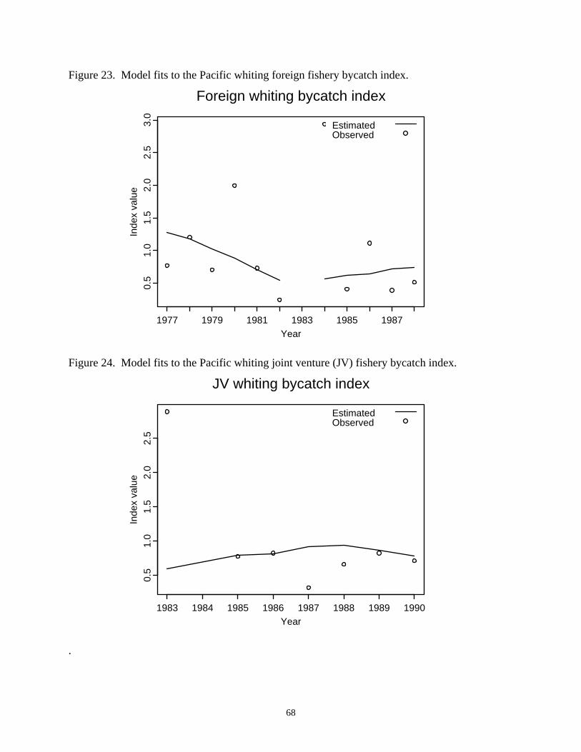
68

Figure 23. Model fits to the Pacific whiting foreign fishery bycatch index.

Year

Inde

x va

lue

1977 1979 1981 1983 1985 1987

0.5

1.0

1.5

2.0

2.5

3.0

Foreign whiting bycatch index

EstimatedObserved

Figure 24. Model fits to the Pacific whiting joint venture (JV) fishery bycatch index.

Year

Inde

x va

lue

1983 1984 1985 1986 1987 1988 1989 1990

0.5

1.0

1.5

2.0

2.5

JV whiting bycatch index

EstimatedObserved

.

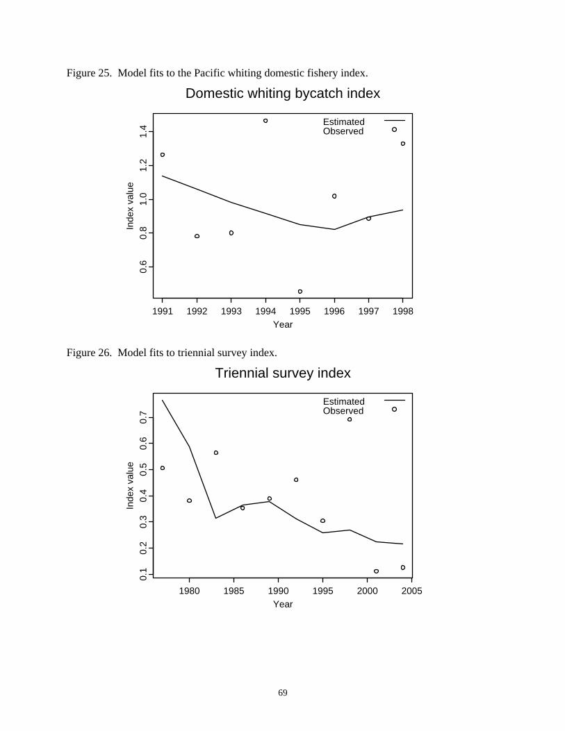
69

Figure 25. Model fits to the Pacific whiting domestic fishery index.

Year

Inde

x va

lue

1991 1992 1993 1994 1995 1996 1997 1998

0.6

0.8

1.0

1.2

1.4

Domestic whiting bycatch index

EstimatedObserved

Figure 26. Model fits to triennial survey index.

Year

Inde

x va

lue

1980 1985 1990 1995 2000 2005

0.1

0.2

0.3

0.4

0.5

0.6

0.7

Triennial survey index

EstimatedObserved

70

Figure 27a. Age composition residuals for the Vancouver-Columbia fishery from the base model. Residuals are standardized differences (observed – estimated). Dark circles are positive residuals and open circles are negative residuals.

2

4

6

8

10

12

14

16

18

20

1979 1982 1985 1988 1991 1994 1997 2000 2003

Year

Age

Vancouver-Columbia fishery (male)

2

4

6

8

10

12

14

16

18

20

1979 1982 1985 1988 1991 1994 1997 2000 2003

Year

Age

Vancouver-Columbia fishery (female)

71

Figure 27b. Age composition residuals for the Oregon midwater trawl fishery from the base model. Residuals are standardized differences (observed – estimated). Dark circles are positive residuals and open circles are negative residuals.

2

4

6

8

10

12

14

16

18

20

1983 1986 1989 1992 1995 1998 2001 2004

Year

Age

Oregon midwater trawl fishery (male)

2

4

6

8

10

12

14

16

18

20

1983 1986 1989 1992 1995 1998 2001 2004

Year

Age

Oregon midwater trawl (female)

72

Figure 27c. Age composition residuals for the Oregon bottom trawl fishery from the base model. Residuals are standardized differences (observed – estimated). Dark circles are positive residuals and open circles are negative residuals.

2

4

6

8

10

12

14

16

18

20

1983 1986 1989 1992 1995 1998

Year

Age

Oregon bottom trawl fishery (male)

2

4

6

8

10

12

14

16

18

20

1983 1986 1989 1992 1995 1998

Year

Age

Oregon bottom trawl fishery (female)

73

Figure 27d. Age composition residuals for the Eureka-Conception fishery from the base model. Residuals are standardized differences (observed – estimated). Dark circles are positive residuals and open circles are negative residuals.

2

4

6

8

10

12

14

16

18

20

1977 1980 1983 1986 1989 1992 1995 1998 2001 2004

Year

Age

Eureka-Conception fishery (male)

2

4

6

8

10

12

14

16

18

20

1977 1980 1983 1986 1989 1992 1995 1998 2001 2004

Year

Age

Eureka-Conception fishery (female)

74

Figure 28. Comparisons of age 3+ biomass between base model of this assessment (2005 base model) and base model of the 2003 assessment.

Year

Bio

mas

s (1

000m

t)

1960 1970 1980 1990 2000

050

100

150

200

250

300

Comparisons between 2003 and 2005 base models

2005 base model2003 base model

Figure 29. Comparisons of age 3+ biomass between base model (T2) and other models.

Year

Bio

mas

s (1

000m

t)

1960 1970 1980 1990 2000

050

100

150

200

250

300

Comparisons between base model (T2) and other models

Model T2Model M011Model T1Model M015

75

Figure 30. Comparisons of estimated age 3 recruitment between base model (T2) and other models.

Year

Age

3 re

crui

t (*1

000)

1960 1970 1980 1990 2000

020

000

6000

010

0000

Comparisons between base model (T2) and other models

Model T2Model M011Model T1Model M015

Figure 31. Comparisons of depletion rates (%) between base model (T2) and other models. Overfished threshold (25%) is also shown.

Year

Dep

letio

n (%

)

1978 1982 1986 1990 1994 1998 2002

020

4060

8010

0

Comparisons between base model (T2) and other models

Model T2Model M011Model T1Model M015

Overfished threshold (25%)

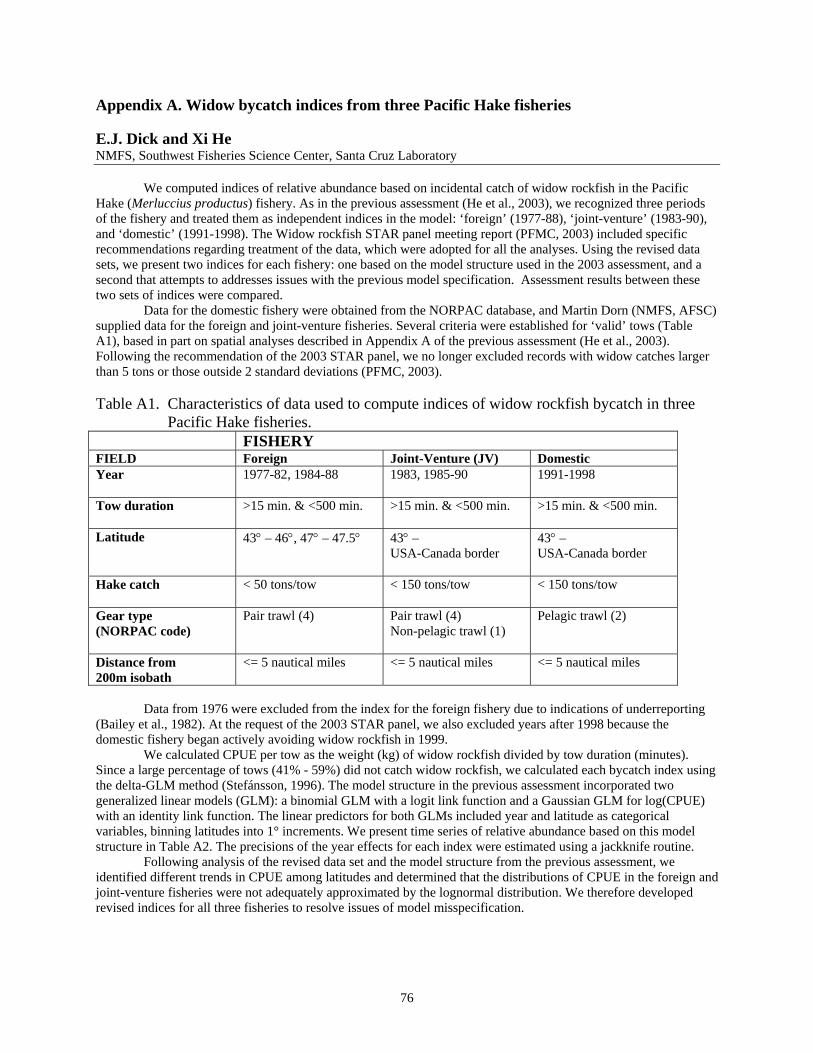
76

Appendix A. Widow bycatch indices from three Pacific Hake fisheries E.J. Dick and Xi He NMFS, Southwest Fisheries Science Center, Santa Cruz Laboratory

We computed indices of relative abundance based on incidental catch of widow rockfish in the Pacific Hake (Merluccius productus) fishery. As in the previous assessment (He et al., 2003), we recognized three periods of the fishery and treated them as independent indices in the model: ‘foreign’ (1977-88), ‘joint-venture’ (1983-90), and ‘domestic’ (1991-1998). The Widow rockfish STAR panel meeting report (PFMC, 2003) included specific recommendations regarding treatment of the data, which were adopted for all the analyses. Using the revised data sets, we present two indices for each fishery: one based on the model structure used in the 2003 assessment, and a second that attempts to addresses issues with the previous model specification. Assessment results between these two sets of indices were compared.

Data for the domestic fishery were obtained from the NORPAC database, and Martin Dorn (NMFS, AFSC) supplied data for the foreign and joint-venture fisheries. Several criteria were established for ‘valid’ tows (Table A1), based in part on spatial analyses described in Appendix A of the previous assessment (He et al., 2003). Following the recommendation of the 2003 STAR panel, we no longer excluded records with widow catches larger than 5 tons or those outside 2 standard deviations (PFMC, 2003). Table A1. Characteristics of data used to compute indices of widow rockfish bycatch in three

Pacific Hake fisheries. FISHERY FIELD Foreign Joint-Venture (JV) Domestic Year 1977-82, 1984-88

1983, 1985-90 1991-1998

Tow duration >15 min. & <500 min. >15 min. & <500 min. >15 min. & <500 min.

Latitude

43° – 46°, 47° – 47.5° 43° – USA-Canada border

43° – USA-Canada border

Hake catch < 50 tons/tow

< 150 tons/tow < 150 tons/tow

Gear type (NORPAC code)

Pair trawl (4)

Pair trawl (4) Non-pelagic trawl (1)

Pelagic trawl (2)

Distance from 200m isobath

<= 5 nautical miles <= 5 nautical miles <= 5 nautical miles

Data from 1976 were excluded from the index for the foreign fishery due to indications of underreporting

(Bailey et al., 1982). At the request of the 2003 STAR panel, we also excluded years after 1998 because the domestic fishery began actively avoiding widow rockfish in 1999.

We calculated CPUE per tow as the weight (kg) of widow rockfish divided by tow duration (minutes). Since a large percentage of tows (41% - 59%) did not catch widow rockfish, we calculated each bycatch index using the delta-GLM method (Stefánsson, 1996). The model structure in the previous assessment incorporated two generalized linear models (GLM): a binomial GLM with a logit link function and a Gaussian GLM for log(CPUE) with an identity link function. The linear predictors for both GLMs included year and latitude as categorical variables, binning latitudes into 1° increments. We present time series of relative abundance based on this model structure in Table A2. The precisions of the year effects for each index were estimated using a jackknife routine.

Following analysis of the revised data set and the model structure from the previous assessment, we identified different trends in CPUE among latitudes and determined that the distributions of CPUE in the foreign and joint-venture fisheries were not adequately approximated by the lognormal distribution. We therefore developed revised indices for all three fisheries to resolve issues of model misspecification.

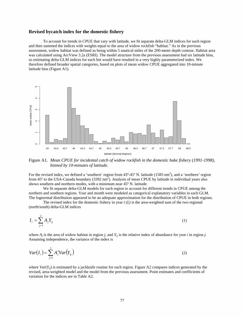
77

Revised bycatch index for the domestic fishery To account for trends in CPUE that vary with latitude, we fit separate delta-GLM indices for each region

and then summed the indices with weights equal to the area of widow rockfish “habitat.” As in the previous assessment, widow habitat was defined as being within 5 nautical miles of the 200-meter depth contour. Habitat area was calculated using ArcView 3.2a (ESRI). The model structure from the previous assessment had six latitude bins, so estimating delta-GLM indices for each bin would have resulted in a very highly parameterized index. We therefore defined broader spatial categories, based on plots of mean widow CPUE aggregated into 10-minute latitude bins (Figure A1).

43 43.3 43.7 44 44.3 44.7 45 45.3 45.7 46 46.3 46.7 47 47.3 47.7 48 48.3

latitude (decimal degrees)

mea

n w

idow

CP

UE

01

23

45

Figure A1. Mean CPUE for incidental catch of widow rockfish in the domestic hake fishery (1991-1998),

binned by 10-minutes of latitude. For the revised index, we defined a ‘southern’ region from 43º-45º N. latitude (1583 nm2), and a ‘northern’ region from 45º to the USA-Canada boundary (3392 nm2). Analysis of mean CPUE by latitude in individual years also shows southern and northern modes, with a minimum near 45º N. latitude.

We fit separate delta-GLM models for each region to account for different trends in CPUE among the northern and southern regions. Year and month were modeled as categorical explanatory variables in each GLM. The lognormal distribution appeared to be an adequate approximation for the distribution of CPUE in both regions.

The revised index for the domestic fishery in year i (Ii) is the area-weighted sum of the two regional (north/south) delta-GLM indices

∑=

=2

1jijji YAI (1)

where Aj is the area of widow habitat in region j, and Yij is the relative index of abundance for year i in region j. Assuming independence, the variance of the index is

( ) ( )∑=

=2

1

2

jijji YVarAIVar (2)

where Var(Yij) is estimated by a jackknife routine for each region. Figure A2 compares indices generated by the revised, area-weighted model and the model from the previous assessment. Point estimates and coefficients of variation for the indices are in Table A2.

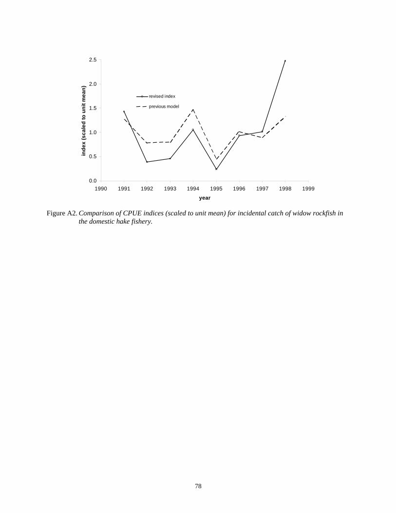
78

0.0

0.5

1.0

1.5

2.0

2.5

1990 1991 1992 1993 1994 1995 1996 1997 1998 1999

year

inde

x (s

cale

d to

uni

t mea

n)

revised index

previous model

Figure A2. Comparison of CPUE indices (scaled to unit mean) for incidental catch of widow rockfish in

the domestic hake fishery.

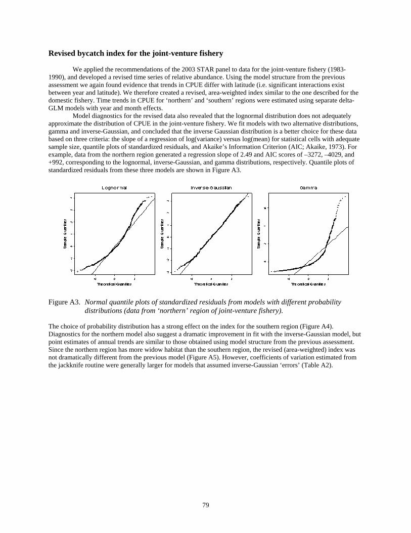
79

Revised bycatch index for the joint-venture fishery We applied the recommendations of the 2003 STAR panel to data for the joint-venture fishery (1983-

1990), and developed a revised time series of relative abundance. Using the model structure from the previous assessment we again found evidence that trends in CPUE differ with latitude (i.e. significant interactions exist between year and latitude). We therefore created a revised, area-weighted index similar to the one described for the domestic fishery. Time trends in CPUE for ‘northern’ and ‘southern’ regions were estimated using separate delta-GLM models with year and month effects.

Model diagnostics for the revised data also revealed that the lognormal distribution does not adequately approximate the distribution of CPUE in the joint-venture fishery. We fit models with two alternative distributions, gamma and inverse-Gaussian, and concluded that the inverse Gaussian distribution is a better choice for these data based on three criteria: the slope of a regression of log(variance) versus log(mean) for statistical cells with adequate sample size, quantile plots of standardized residuals, and Akaike’s Information Criterion (AIC; Akaike, 1973). For example, data from the northern region generated a regression slope of 2.49 and AIC scores of –3272, –4029, and +992, corresponding to the lognormal, inverse-Gaussian, and gamma distributions, respectively. Quantile plots of standardized residuals from these three models are shown in Figure A3.

Figure A3. Normal quantile plots of standardized residuals from models with different probability

distributions (data from ‘northern’ region of joint-venture fishery).

The choice of probability distribution has a strong effect on the index for the southern region (Figure A4). Diagnostics for the northern model also suggest a dramatic improvement in fit with the inverse-Gaussian model, but point estimates of annual trends are similar to those obtained using model structure from the previous assessment. Since the northern region has more widow habitat than the southern region, the revised (area-weighted) index was not dramatically different from the previous model (Figure A5). However, coefficients of variation estimated from the jackknife routine were generally larger for models that assumed inverse-Gaussian ‘errors’ (Table A2).

80

0.0

0.5

1.0

1.5

2.0

2.5

3.0

3.5

4.0

1982 1983 1984 1985 1986 1987 1988 1989 1990 1991

Year

scal

ed d

elta

-GLM

inde

x

inverse-Gaussianlognormal

Figure A4. CPUE indices (scaled to unit mean) based on different assumptions about the distribution of

‘errors.’ Data are widow bycatch in the joint-venture hake fishery, southern region (latitudes 43-45).

0.0

0.5

1.0

1.5

2.0

2.5

3.0

3.5

1982 1983 1984 1985 1986 1987 1988 1989 1990 1991

year

scal

ed d

elta

-GLM

inde

x revisedprevious

Figure A5. CPUE indices (scaled to unit mean) for incidental catch of widow rockfish in the joint-

venture hake fishery.

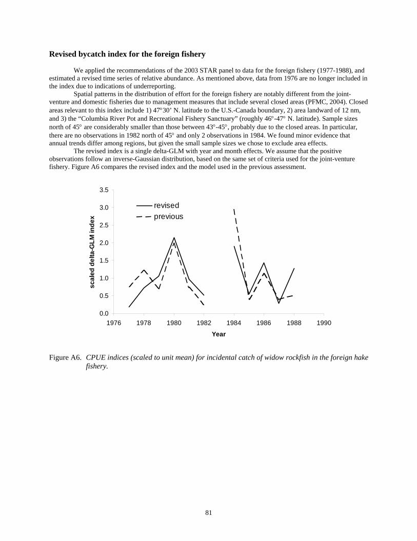
81

Revised bycatch index for the foreign fishery We applied the recommendations of the 2003 STAR panel to data for the foreign fishery (1977-1988), and

estimated a revised time series of relative abundance. As mentioned above, data from 1976 are no longer included in the index due to indications of underreporting.

Spatial patterns in the distribution of effort for the foreign fishery are notably different from the joint-venture and domestic fisheries due to management measures that include several closed areas (PFMC, 2004). Closed areas relevant to this index include 1) 47°30’ N. latitude to the U.S.-Canada boundary, 2) area landward of 12 nm, and 3) the “Columbia River Pot and Recreational Fishery Sanctuary” (roughly 46°-47° N. latitude). Sample sizes north of 45° are considerably smaller than those between 43°-45°, probably due to the closed areas. In particular, there are no observations in 1982 north of 45° and only 2 observations in 1984. We found minor evidence that annual trends differ among regions, but given the small sample sizes we chose to exclude area effects.

The revised index is a single delta-GLM with year and month effects. We assume that the positive observations follow an inverse-Gaussian distribution, based on the same set of criteria used for the joint-venture fishery. Figure A6 compares the revised index and the model used in the previous assessment.

0.0

0.5

1.0

1.5

2.0

2.5

3.0

3.5

1976 1978 1980 1982 1984 1986 1988 1990

Year

scal

ed d

elta

-GLM

inde

x

revisedprevious

Figure A6. CPUE indices (scaled to unit mean) for incidental catch of widow rockfish in the foreign hake

fishery.

82

Table A2. Indices of relative abundance based on incidental catch of widow rockfish in three Pacific Hake fisheries. Indices scaled to unit mean.

Fishery 2003 Model Structure Revised Model Structure Scaled Index CV Scaled Index CV Domestic

1991 1992 1993 1994 1995 1996 1997 1998

1.264 0.781 0.801 1.465 0.455 1.018 0.886 1.330

0.125 0.125 0.104 0.068 0.106 0.082 0.077 0.079

1.433 0.386 0.457 1.057 0.239 0.935 1.016 2.478

0.170 0.139 0.204 0.155 0.145 0.190 0.158 0.187

Joint-Venture

1983 1985 1986 1987 1988 1989 1990

2.889 0.776 0.823 0.320 0.659 0.824 0.710

0.120 0.117 0.081 0.087 0.077 0.064 0.074

1.995 1.052 1.132 0.382 0.621 0.698 1.120

0.332 0.443 0.294 0.302 0.337 0.270 0.306

Foreign

1977 1978 1979 1980 1981 1982 1984 1985 1986 1987 1988

0.770 1.205 0.703 1.993 0.728 0.243 2.937 0.407 1.111 0.390 0.513

0.115 0.112 0.119 0.131 0.126 0.247 0.125 0.107 0.103 0.088 0.124

0.186 0.726 1.062 2.148 0.962 0.520 1.891 0.543 1.425 0.273 1.264

0.409 0.582 0.630 0.985 0.523 0.933 0.464 0.572 0.508 0.283 0.603

83

Comparisons of assessment results between two indices We applied two sets of indices to the Model 4 assessment model (see main document), and compared the

assessment results between them. Overall, the results were very similar, including trends in biomass, spawning outputs, and recruitments. Graphic comparisons of the assessment results are not presented because they are similar. Comparisons of key assessment results are presented in Table A3. Table A3. Comparisons of key assessment results between two indices.

Parameter and estimate Previous index Revised index Steepness (h) 0.2810 0.2814 Unfished spawning output (B0) (million of eggs) 49676 49442 Current spawning output (Bt) (million of eggs) 15444 15264 Depletion (100*Bt/B0) 31.09 30.87

References Akaike, H., 1973. Information theory as an extension of the maximum likelihood principle. In: Petrov, B., Csaki, F.

(Eds.), Second International Symposium on Information Theory. Akademiai Kiado, Budapest, pp. 267–281.

Bailey, K., R. C. Francis, and P. R. Stevens. 1982. The life history and fishery of Pacific whiting, Merluccius

productus. California Cooperative Oceanic Fisheries Investigations Reports 23:81-98. Environmental Systems Research Institute (ESRI). Redlands, CA. http://www.esri.com. He, X., S. Ralston, A. MacCall, D. Pearson, and E. Dick. 2003. Status of the widow rockfish resource in 2003.

Pacific Fishery Management Council, Portland, Oregon. Pacific Fishery Management Council. 2003. Widow rockfish STAR panel meeting report. Pacific Fishery

Management Council, Portland, OR. Pacific Fishery Management Council. 2004. Pacific Coast Groundfish Fishery Management Plan for the California,

Oregon, and Washington Groundfish Fishery as Amended through Amendment 17. Pacific Fishery Management Council, Portland, OR.

Stefánsson, G. 1996. Analysis of groundfish survey abundance data: Combining the GLM and delta approaches.

ICES Journal of Marine Science 53(3):577-588.

84

Appendix B: Triennial trawl survey estimates of widow rockfish abundance John Field, E.J. Dick and Xi He NMFS, Southwest Fisheries Science Center, Santa Cruz Laboratory Introduction Widow rockfish are poorly sampled by the West Coast triennial trawl survey due to a combination of factors. These include their tendency to form dense midwater schools from dusk until dawn, often over irregular bottom habitat, and to often disperse or move closer to the bottom during daylight (Wilkins 1986, Stanley et al. 2000). Although the habitat associations of most Sebastes species present problems that are faced in estimating relative abundance time series from the triennial survey (Jagielo et al. 2003, Zimmerman et al. 2003), widow rockfish pose particular challenges. For example Millar and Methot (2002) performed a hierarchical analysis of survey catchabilities for six Sebastes stocks using traditional swept-area biomass estimates in the triennial survey, and found strong evidence that widow rockfish have a considerably lower catchability than other Sebastes stocks (on the order of 0.05, as opposed to 0.2 for several other species). As a consequence of these problems, triennial survey data have only sporadically been included in past widow rockfish assessments, generally with poor results and little to no improvement in model behavior. For example, Williams (2000) found that the triennial trawl survey data appeared to be in conflict with both the midwater trawl survey and the Oregon logbook index. However as the ability to use fishery-dependent indices of abundance has become problematic in recent years, as a result bias introduced by regulatory changes, the need to develop fishery-independent time series of abundance has become greater. The patchiness of widow rockfish catches in the triennial trawl survey is particularly problematic. Table 1 and Figure 1 show the area-swept biomass estimates of widow rockfish over time using the traditional method of estimation (M. Wilkins, pers. com.). Figure 2 shows the expanded length-frequency compositions from the survey. These estimates suggest very low biomass levels in the early part of the time series, increasing to a peak level of abundance in 1992, and declining thereafter; and are inconsistent with time series trends from alternative indices of abundance and from recent stock assessments. However of the 4025 tows done between 55 and 366 meters depth (excluding tows in Canadian waters), half of the total biomass of widow rockfish caught in the survey were caught in only five, with the largest tow in 1992 (almost solely responsible for the tremendously high area-swept biomass index in that year, as this tow occurred in a strata with a large area) and the second and third largest in 1989. Over 65% of the total catches of widow rockfish were in just ten tows. Figure 3 shows the relative distribution of CPUE values for the 4025 triennial survey tows used in this analysis. By contrast, for yellowtail rockfish (S flavidus) there were 41 tows with catches greater than 100 kg, and 163 tows with between 10 and 100 kg of catch. Figure 4 shows the distribution of triennial survey tows and corresponding catches of widow rockfish for the years 1977-2004, within the 55 to 366 meter depth strata.

85

Data and Methods In order to respond to the 2003 STAR Panel request that the widow rockfish assessment try to incorporate data from the triennial survey, we evaluated whether a more appropriate time series could be generated using the triennial survey data using a delta-GLM modeling approach. We obtained haul-specific triennial survey data from 1977 to 2004 from M. Wilkins (AFSC), and removed both bad performance tows and tows that were retrospectively labeled as “waterhauls” in the analysis by Zimmerman et al. (2001). We included all subsequent tows that occurred between depths of 55 to 366 meters for all years, with the exception of a small number of tows made south of 34˚ 30 in 1977, and all tows north of 48˚ 20’ (Canadian waters). A cumulative frequency plot showing both positive tows and cumulative total survey catch (CPUE) by latitude for this region is presented as Figure 5a, which demonstrate that widow rockfish are widely dispersed along the coastline of the area sampled by the survey. Figure 5b shows the same tow data, with the cumulative frequency of CPUE and the number of positive tows by depth. As these data are characterized by a large proportion (~88%) of zero observations and highly skewed positive observations, they are appropriate candidates for the delta-GLM method, which has become an increasingly accepted means for generating relative abundance time series for other fish populations (Lo et al. 1992, Dick 2004, Maunder and Punt 2004). This method is based on the product of fitted values from two GLMs; a binomial GLM that estimates the probability of a positive observation, p, and a second GLM that estimates the mean, µ, of all positive observations. The framework allows for both the evaluation of alternative link functions (logit, probit) for the binomial model, and alternative error distributions (lognormal, gamma) to be evaluated from the positive data. The final index of abundance is the product of the year effects from these two models, pµ. The model used here was developed in the R programming language by Dick (2004), and has been referred to earlier in both this assessment and previous assessments (He et al. 2003). Akaike’s information criterion (AIC) is used to assess whether the various factors (year, strata) are able to explain the variability in the data, such that the model with the smallest AIC is best supported by the data. A series of models were run to evaluate both alternative factors and alternative link functions and error distributions. The prime candidates for factors included the traditional triennial survey strata (55 to 183 m; 184-366 meters, in different latitudinal configurations along the coast, see Weinberg et al. 2002), independent depth and latitude factors created using 50 meter depth and 2° latitude bins (similar to Ralston et al. 1998), and categorizing tows as being either within five nautical miles (inshore or offshore) of the shelf break (as with the Pacific whiting fishery index described earlier). Additionally, models were explored that used either finer or courser depth and latitude bins, that either included or excluded deeper (>300m) and/or shallow (<100m) tows, that weighted data with relative areas of their strata, that used sea surface temperature (SST) data as a covariate, that evaluated the interaction between El Niño and widow rockfish catchability, and that excluded the 1977 survey data. Although stock assessment authors were cautioned against using 1977 triennial survey data, due to the fact that this first survey fished only depths greater than 90 meters (NWFSC, unpublished report), the results here (including Figures 4a and 8a) strongly suggests that widow rockfish are very rarely encountered shallower than 100 meters. This result is consistent with Reynolds (2003) who used Oregon commercial logbook data to demonstrate that widow rockfish were strongly associated with habitats between 136 and 298

86

meters depth. Consequently we believe that the inclusion of the 1977 survey data is appropriate for this stock. Results Survey indices In all configurations, both the binomial and the positive components of the Delta-GLM explained a very modest proportion of the variability in the data. However, the resulting trends for both year effects and spatial factors (latitude, depth, strata) were consistent across models. The lognormal distribution was determined to be appropriate based on a comparison of AIC scores with the gamma distribution (the latter was nearly 200 points greater); the inverse gaussian model for positives was unable to converge. Evaluation of the link functions for the binomial model using AIC criteria did not suggest a meaningful distinction among the three possibilities (logit, probit, or cloglog), in all instances the differences were less than 1 AIC point (and generally less than 0.5 points) apart. The logit was used as the default link function for all subsequent models. For simplicity, only select results are shown here. These include a base model that uses coastwide data with 2° latitude and 50m depth bins, and an alternative model that excludes the 50 to 100 m depth range, and only considers data north of 41° latitude (both of these are presented with and without inclusion of the 1977 data). The latter model is shown as an example of the models that “best” fit the data, which were those that excluded both the shallow, nearshore tows (which had very few positives), and those that excluded tows south of 41° latitude. Table 2 shows the year effects for all four models, with standard errors estimated by a jackknife routine and coefficients of variation for the first model in each of the two cases. Differences in the standard errors for the models excluding 1977 were negligible. Figure 6 shows the results from Table 2 for the two base models. While the SST data from the survey were uninformative, both the published literature (Woodbury 1999, Reynolds 2003) and the observation that catches and catch rates tended to be higher during strong El Niño events (1982-83, 1992-94 and 1997-98; based on the multivariate El Niño index, or MEI; http://www.cdc.noaa.gov/people/klaus.wolter/MEI/table.html) led us to evaluate potential interactions with widow rockfish availability and the MEI. First, we show the apparent relationship between the base model and the MEI (Figure 6), in which the R2 value between the detrended index and the average MEI in the 12 month period immediately preceding the survey is 0.547 (P=0.015). Accounting for this relationship in the Delta-GLM model was compromised by the fact that these events were (essentially) on an annual scale. However, by running the model without year effects, but with a “dummy” variable for El Niño effects (e.g., either positive or negative), we found that a reasonable amount of the variance in the data could be explained by this factor (improvement of approximately 2 AIC points for the positives model, 9 AIC points for the binomial model). Moreover, the effect was to roughly double the abundance index during El Niño years (a ratio of 1.87 for El Niño versus non- El Niño years). There were insufficient data to evaluate fish were less available during strong La Niña events, as only one triennial survey (1989) occurred during strongly negative MEI (eg., La Niña) conditions.

87

Consequently, we present two alternative models in which the consequences of El Niño are accounted for in what is admittedly an imperfect manner. We considered two ways of approaching this issue. In the first, the model is simply run without the years of a strong MEI (e.g., excluding 1983, 1992 and 1998). The results are only slightly different from the base model for the remaining years. In the second approach, we modified the year index for years with a strong positive MEI by scaling these years by the reciprocal of the El Niño factor (e.g., 1/1.87) to account for increased availability during warm years. The results of these two models are presented in Table 3 and Figure 7 (note that alternative model 3 values in Table 3 are simply the same as the base model, but scaled by El Nino years). With respect to the depth and latitude effects, Table 4 shows the indices for the base model, and Figures 8a and 8b show these results graphically. Table 5 shows the AIC scores for both the binomial and the positive components of the two models, with sequentially added combinations of model factors. The improvement in AIC is modest in the first base model, using depth and latitude bins, particularly for the year effects in the binomial model and all effects in the positives model. In the alternative model 1, the improvement in AIC is considerably greater for the positive model, and roughly similar for the binomial model. For all models, when Bayes Information Criteria (BIC) is used rather than AIC, including the year effects as explanatory variables are not supported by the data, although the latitude and depth factors remain acceptable. Although BIC selects more parsimonious models than AIC for large datasets, the relatively small number of parameters and the a priori expectation that the data will not be well explained by any model, make interpretation of these results somewhat subjective. These models were also tested for interactions among year and area effects, none of which were apparent in these models (including the model that was used to estimate the El Niño effect). Finally, diagnostic plots for the goodness of fit of each of the positive models for the base model are presented as Figures 9. Comparisons of assessment results Table 6 shows comparisons of key assessment results between base model and alternative model 1. The results of base model seem to be more comparable to results of other models in the main document (Table 14, Model 1, 2, 3, and 5), in terms of stock depletion rate. The base model also had better fits in the assessment model (negative log likelihood value = 188.17) than the alternative model (negative log likelihood value = 191.71). Discussion and Conclusions There is no doubt that the ability of the triennial trawl survey to provide a reliable index of relative abundance for widow rockfish is severely compromised, largely as a result of the atypical patterns of habitat preferences and aggregation demonstrated by the species, as well as a result of anomalous behavior during El Niño conditions. As suggested earlier, Reynolds (2003) used Oregon trawl logbook data to describe widow rockfish habitat; she found significant habitat associations included bottom depths of 136 to 298 meters, vertical depths of 101 to 197 meters, and temperatures between 7.1 and 8.1°C. Importantly, she also found that 1992 and 1997 were two years for which significant bottom depth associations were not detected, and no significant

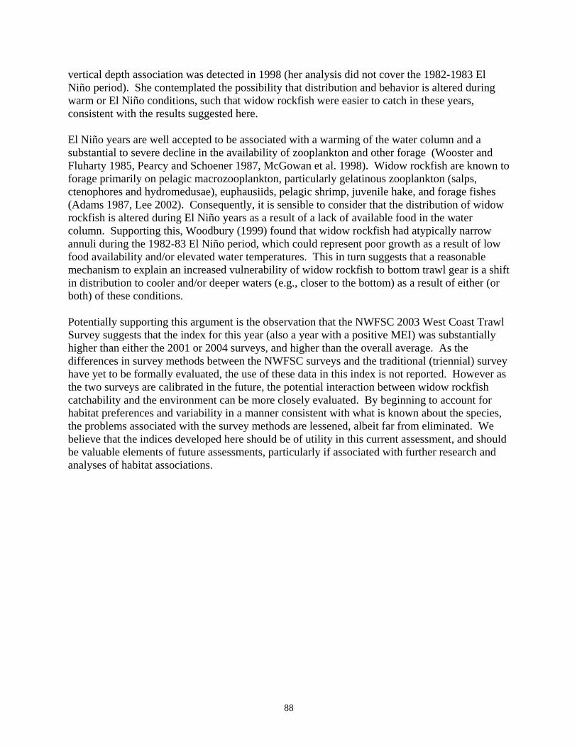
88

vertical depth association was detected in 1998 (her analysis did not cover the 1982-1983 El Niño period). She contemplated the possibility that distribution and behavior is altered during warm or El Niño conditions, such that widow rockfish were easier to catch in these years, consistent with the results suggested here. El Niño years are well accepted to be associated with a warming of the water column and a substantial to severe decline in the availability of zooplankton and other forage (Wooster and Fluharty 1985, Pearcy and Schoener 1987, McGowan et al. 1998). Widow rockfish are known to forage primarily on pelagic macrozooplankton, particularly gelatinous zooplankton (salps, ctenophores and hydromedusae), euphausiids, pelagic shrimp, juvenile hake, and forage fishes (Adams 1987, Lee 2002). Consequently, it is sensible to consider that the distribution of widow rockfish is altered during El Niño years as a result of a lack of available food in the water column. Supporting this, Woodbury (1999) found that widow rockfish had atypically narrow annuli during the 1982-83 El Niño period, which could represent poor growth as a result of low food availability and/or elevated water temperatures. This in turn suggests that a reasonable mechanism to explain an increased vulnerability of widow rockfish to bottom trawl gear is a shift in distribution to cooler and/or deeper waters (e.g., closer to the bottom) as a result of either (or both) of these conditions. Potentially supporting this argument is the observation that the NWFSC 2003 West Coast Trawl Survey suggests that the index for this year (also a year with a positive MEI) was substantially higher than either the 2001 or 2004 surveys, and higher than the overall average. As the differences in survey methods between the NWFSC surveys and the traditional (triennial) survey have yet to be formally evaluated, the use of these data in this index is not reported. However as the two surveys are calibrated in the future, the potential interaction between widow rockfish catchability and the environment can be more closely evaluated. By beginning to account for habitat preferences and variability in a manner consistent with what is known about the species, the problems associated with the survey methods are lessened, albeit far from eliminated. We believe that the indices developed here should be of utility in this current assessment, and should be valuable elements of future assessments, particularly if associated with further research and analyses of habitat associations.

89

Sources Adams, P.B. 1987. Diet of widow rockfish (Sebastes entomelas) in northern California. In W.H. Lenarz and D.R. Gunderson (editors) Widow rockfish: proceedings of a workshop. NOAA Technical Report NMFS 48. Dick, E.J. 2004. Beyond ‘lognormal versus gamma’: discrimination among error distributions for generalized linear models. Fisheries Research 70: 351-366. He, X., S.V. Ralston, A.D. MacCall, D.E. Pearson, and E.J. Dick. 2003. Status of the widow rockfish resource in 2003. in Volume I: Status of the Pacific Coast Groundfish Fishery Through 2003 Stock Assessment and Fishery Evaluation Pacific Fishery Management Council: Portland OR. Jagielo, T., A. Hoffman, J. Tagart and M. Zimmermann. 2003. Demersal groundfish densities in trawlable and untrawlable habitats off Washington: implications for the estimation of habitat bias in trawl surveys. Fishery Bulletin 101: 545-565. Lee, Y.W. 2002. Oceanographic effect on the dynamics of food habits and growth conditions of some groundfish species of the Pacific Northwest. Doctoral Dissertation, Oregon State University. Lo, N.C., Jacobson, L.D., and Squires, J.L. 1992. Indices of relative abundance for fish spotter data based on delta-lognormal models. Canadian Journal of Fisheries and Aquatic Sciences 49: 2515-2526. Maunder, M.N. and A.E. Punt. 2004. Standardizing catch and effort data: a review of recent approaches. Fisheries Research 70: 141-159. McGowan, J.A., D.R. Cayan and L.M. Dorman. 1998. Climate, ocean variability and ecosystem response in the Northeast Pacific. Science 281: 210-217. Millar, R.B. and R.D. Methot. 2002. Age-structured meta-analysis of U.S. West Coast rockfish (Scorpaenidae) populations and hierarchical modeling of trawl survey catchabilities. Canadian Journal of Fisheries and Aquatic Sciences 59: 383-392. Northwest Fisheries Science Center. Unpublished report. A summary report from the West Coast groundfish data workshop held July 26-30, 2004 in Seattle, WA. Pearcy, W.G.and A. Schoener. 1987. Changes in the marine biota coincident with the 1982-1983 El Nino in the northeastern Subarctic Pacific Ocean. Journal of Geophysical Research 92: 14417-14428. Philips, J.B. 1964. Life history studies on ten species of rockfish (genus Sebastodes). California Department of Fish and Game Fish Bulletin 126. 63 p.

90

Ralston, S.V., D. Pearson, J. Reynolds. 1998. Status of the chilipepper rockfish in 1998. In Appendix to Status of the Pacific Coast Groundfish Fishery through 1998 and recommended acceptable biological catches for 1999. Stock Assessment and Fishery Evaluation. Pacific Fishery Management Council: Portland OR. Reynolds, J.A. 2003. Quantifying habitat associations in marine fisheries: a generalization of the Kolmogorov-Smirnov statistic using commercial logbook records linked to archived environmental data. Canadian Journal of Fisheries and Aquatic Sciences 60: 370-378. Stanley, R.D., R. Kieser, K. Cooke, A.M. Surry, and B. Mose. 2000. Estimation of a widow rockfish (Sebastes entomelas) shoal off British Columbia, Canada as a joint exercise between stock assessment staff and the fishing industry. ICES Journal of Marine Science 57: 1035-1049. Weinberg, K.L., M.E. Wilkins, F.R. Shaw, and M. Zimmerman. 2002. The 2001 Pacific West Coast bottom trawl survey of groundfish resources: Estimates of distribution, abundance, and length and age composition. NOAA Technical Memorandum NMFS-AFSC-128. Wilkins, M.E. 1986. Development and evaluation of methodologies for assessing and monitoring the abundance of widow rockfish, Sebastes entomelas. Fishery Bulletin 84: 287-310. Williams, E.H., A.D. MacCall, S.V. Ralston and D.E. Pearson. 2000. Status of the widow rockfish resource in Y2K. In Appendix to the status of the Pacific coast groundfish fishery through 2001 and acceptable biological catches for 2002: Stock assessment and fishery evaluation. Pacific Fishery Management Council: Portland, Oregon. Woodbury, D. 1999. Reduction of growth in otoliths of widow and yellowtail rockfish (Sebastes entomelas and S. flavidus) during the 1983 El Niño. Fishery Bulletin 97: 680-689. Wooster, W.S. and D.L. Fluharty (editors) El Niño North: Niño Effects in the Eastern Subarctic Pacific Ocean. Washington Sea Grant: Seattle. Zimmerman, M., M.E. Wilkins, K.L. Weinberg, R.R. Lauth, and F.R. Shaw. 2001. Retrospective analysis of suspiciously small catches in the National Marine Fisheries Service West Coast triennial bottom trawl survey. AFSC Processed Report 2001-03. Zimmerman, M., M.E. Wilkins, K.L. Weinberg, R.R. Lauth, and F.R. Shaw. 2003. Influence of improved performance monitoring on the consistency of a bottom trawl survey. ICES Journal of Marine Science 60, 818-826.

91

Table 1: Triennial trawl survey biomass estimates for widow rockfish from 1977-2004.

depth USyear strata Vancouver Columbia Eureka Monterey Conception U.S. total1977 91-366 m Biomass 844 362 8 195 154 1111

CV 0.79 0.29 0.52 0.41 0.91 0.611980 55-366 m Biomass 0 1175 228 249 N/A 1652

CV - 0.77 0.58 0.69 N/A 0.561983 55-366 m Biomass 1879 909 267 392 N/A 3447

CV 1.00 0.55 0.46 0.58 N/A 0.571986 55-366 m Biomass 44 1413 1094 2346 N/A 4897

CV 0.55 0.78 0.78 0.85 N/A 0.631989 55-366 m Biomass 3533 614 2205 826 2129 9307

CV 0.98 0.70 0.99 0.88 1.00 0.501992 55-366 m Biomass 297 626 22 11526 708 13178

CV 0.62 0.47 0.54 0.94 1.00 0.821995 55-366 m Biomass 20 2315 90 584 11 3020

CV 0.69 0.99 0.59 0.56 0.64 0.761998 55-366 m Biomass 2241 293 97 1712 0 4343

CV 0.49 0.28 0.34 0.50 1.00 0.322001 55-366 m Biomass 53 102 41 20 10 224

CV 0.70 0.48 0.47 0.84 0.70 0.302004 55-366 m Biomass 27 57 281 488 16 868

CV 0.82 0.49 0.65 0.72 0.85 0.46

92

Table 2: Year effects, standard errors, coefficients of variation, positive and binomial indices, and results that exclude 1977 for the base model and alternative model 1.

Table 3: Year effects, standard errors, coefficients of variation, and the positive and binomial indices for the two alternative models that account for ENSO effects.

Table 4: Latitude and depth effects for base model 1.

Base model Alternative modelindex jack.se CV pos bin no 1977 index jack.se CV pos bin no 1977

1977 0.506 0.125 0.247 3.00 0.169 0.793 0.252 0.318 3.86 0.2051980 0.382 0.127 0.332 2.66 0.143 0.460 0.406 0.182 0.449 3.52 0.115 0.4721983 0.565 0.163 0.289 3.32 0.170 0.683 0.609 0.191 0.313 3.28 0.185 0.6861986 0.353 0.124 0.351 2.53 0.140 0.428 0.294 0.103 0.349 1.68 0.175 0.3321989 0.390 0.186 0.477 3.73 0.105 0.463 0.577 0.360 0.623 6.58 0.088 0.6731992 0.461 0.168 0.364 2.86 0.161 0.553 0.470 0.173 0.368 2.98 0.158 0.5501995 0.305 0.097 0.317 2.57 0.119 0.355 0.265 0.123 0.464 2.73 0.097 0.2911998 0.692 0.216 0.313 3.88 0.179 0.815 0.744 0.231 0.310 2.84 0.262 0.8332001 0.112 0.039 0.350 1.39 0.081 0.129 0.169 0.067 0.394 1.67 0.101 0.1822004 0.126 0.058 0.461 1.09 0.115 0.149 0.094 0.059 0.623 0.72 0.130 0.104

latitude effects depth effects34 0.237 50 0.0436 0.403 100 0.3738 0.449 150 0.9140 0.866 200 1.0142 0.386 250 0.4744 0.159 300 0.2046 0.227

Alternative 2: No Niño years Alt. Model 3: Scale Niño years by Niño factorindex jack.se CV pos bin scalar index jack.se CV pos bin

1977 0.581 0.172 0.295 3.36 0.173 0.506 (all other values assumed 1980 0.411 0.149 0.363 2.76 0.149 0.382 be the same, or scaled 1983 0.534 0.302 similarly to year index, 1986 0.379 0.145 0.383 2.69 0.141 0.353 as the base model)1989 0.419 0.217 0.518 4.03 0.104 0.3901992 0.534 0.2461995 0.303 0.107 0.352 2.54 0.119 0.3051998 0.534 0.3692001 0.111 0.042 0.379 1.38 0.081 0.1122004 0.125 0.058 0.468 1.07 0.117 0.126

93

Table 5a: Parameters, deviance, and AIC scores for base model.

Table 5b: Parameters, deviance, and AIC scores for alternative model 1.

Table 5c: Parameters, deviance, and AIC scores for alternative model 2.

Base model AIC scores positive model binomial modeldf deviance AIC df deviance AIC

no factors 1579 1967.9 no factors 2981.0 2983.0year only 9 1520.6 1967.5 year only 9 2942.5 2962.5

lat only 6 1536.1 1966.4 lat only 6 2934.4 2948.4depth only 5 1522.6 1960.1 depth only 5 2723.2 2735.2all factors 20 1431.0 1959.7 all factors 20 2648.2 2690.0

Alternative Model AIC scores positive model binomial modeldf deviance AIC df deviance AIC

no factors 909.1 1193.8 no factors 1731.0 1733.2year only 9 842.9 1189.0 year only 9 1695.4 1715.4

lat only 3 850.5 1179.7 lat only 3 1704.5 1712.5depth only 4 909.1 1193.8 depth only 4 1635.6 1645.6all factors 16 781.0 1172.0 all factors 16 1575.1 1609.1

Alternative Model 2 AIC scores positive model binomial modeldf deviance AIC df deviance AIC

no factors 1014.0 1248.1 no factors 1934.0 1935.8year only 6 1013.9 1248.1 year only 6 1903.4 1917.4

lat only 6 974.9 1247.9 lat only 6 1901.1 1915.1depth only 5 979.5 1247.4 depth only 5 1801.3 1813.3all factors 17 926.4 1244.2 all factors 17 1750.6 1786.6

94

Table 6 Comparisons of key assessment results between base model and alternative models.

Parameter and estimate Base modelAlternative

model 1 Alternative

model 2 Alternative

model 3 Steepness (h) 0.2810 0.2793 0.749 0.2771 Unfished spawning output (B0) (million of eggs) 49676 49513

48083

49722

Current spawning output (Bt) (million of eggs) 15444 15070

13111

15055

Depletion (100*Bt/B0) 31.09 30.44 27.27 30.28 Figure 1: Triennial trawl survey swept-area biomass estimates of widow rockfish, 1977-2004, for the Monterey through U.S. Vancouver INPFC statistical areas.

0

5000

10000

15000

20000

25000

1977 1980 1983 1986 1989 1992 1995 1998 2001 2004

biom

ass

(ton

s)

95

Figure 2: Percent length frequency compositions from triennial survey index.

1977

0

2

4

6

8

10

12

200 250 300 350 400 450 500

malesfemales

1980

0

2

4

6

8

10

12

14

200 250 300 350 400 450 500

1983

0

2

4

6

8

10

200 250 300 350 400 450 500

1986

0

2

4

6

8

10

200 250 300 350 400 450 500

1989

0

2

4

6

8

10

12

200 250 300 350 400 450 500

1992

0

2

4

6

8

10

12

200 250 300 350 400 450 500

1995

0

2

4

6

8

10

200 250 300 350 400 450 500

1998

0

2

4

6

8

10

200 250 300 350 400 450 500

2001

0

2

4

6

8

10

200 250 300 350 400 450 500

2004

0

2

4

6

8

10

200 250 300 350 400 450 500

96

Figure 3: Binned frequency distribution, in log scale, of triennial survey CPUE values, and percentage of total relative catch represented by bin (note that 22 tows had CPUE values greater than 0 but less than 0.1)

3557

312111 35 10

0500

1000150020002500300035004000

0 0.1 1 10 100

CPUE (kg/ha)

num

ber o

f tow

s

0

20

40

60

80

% o

f tot

al C

PUE

97

Figure 4: Locations of triennial trawl survey tows (1977-2004) and associated CPUE estimates of widow rockfish, for the Monterey through U.S. Vancouver INPFC statistical areas.

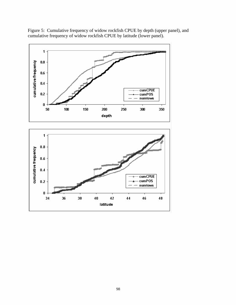
98

Figure 5: Cumulative frequency of widow rockfish CPUE by depth (upper panel), and cumulative frequency of widow rockfish CPUE by latitude (lower panel).

99

Figure 6: Model results from the baseline model and alternative model 1. Figure 7: Widow rockfish base model index and 13 month running mean for the Multivariate ENSO Index (MEI).

-2

-1.5

-1

-0.5

0

0.5

1

1.5

2

2.5

1970 1975 1980 1985 1990 1995 2000 2005

Mul

tivar

iate

ENS

O In

dex

0

0.1

0.2

0.3

0.4

0.5

0.6

0.7

0.8

Trie

nnia

l sur

vey

inde

x

0

0.1

0.2

0.3

0.4

0.5

0.6

0.7

0.8

0.9

1977 1980 1983 1986 1989 1992 1995 1998 2001 2004

base model alternative 1

100

Figure 8: Results from Alternative models 2 and 3, with base model for comparative purposes.

0.0

0.1

0.2

0.3

0.4

0.5

0.6

0.7

0.8

1977 1980 1983 1986 1989 1992 1995 1998 2001 2004

alternative 2 alternative 3 base model

101

Figure 9a: Depth effects (in meters) from the depth and latitude binned base model Figure 9b: Latitude effects from the depth and latitude binned base model (34 represents 34° to 36° latitude, etc)

0.0

0.2

0.4

0.6

0.8

1.0

50 100 150 200 250 300

0.0

0.2

0.4

0.6

0.8

1.0

34 36 38 40 42 44 46

102

Figure 10. Diagnostics of the goodness of fit of the positive model for the base model.

103

Appendix C: Description of assessment model The widow population is assumed to be subject to four fisheries in two regions. Region 1 consists of the Vancouver-Columbia trawl fishery, Oregon midwater trawl fishery, and Oregon bottom trawl fishery. Region 2 consists of the Eureka-Monterey-Conception trawl fishery. Initial condition and cohort growth:

Initial conditions of the population are numbers of fish at sex x , at age a and at the first model year ( y = 0) in 1958, which is given by:

1min

,0, ,0, 1 min max

,0, 1max

0.5 if

if

if 1

x

x

x

R

Mx a x a

Mx a

M

Re a a

N N e a a a

N ea a

e

δ

−−

−−

−

⎧⎪ =⎪⎪⎪= < <⎨⎪⎪⎪ =⎪ −⎩

( 10)

where R = mean recruitment 1Rδ = recruitment residual at year 0

mina = age of recruitment (minimum age in model)

maxa = maximum age, including age-plus groups

xM = natural mortality for sex x , which is constant across year and age Numbers of fish in subsequent years are given by:

, 1, 1

, 1,

min

, , , 1, 1 min max

, 1, 1

0.5 if

if

y

fx x y a

f

x x y

R

M F

x y a x y a

M F

x y a

Re a a

N N e a a a

N e

δ

− −

−

⎛ ⎞⎜ ⎟− +⎜ ⎟⎝ ⎠

− −

− +

− −

=

∑= < <

1 , 1, max

max, 1, max+ if f f

xa x y af f

M F

x y aN e a a− −

⎛ ⎞ ⎛ ⎞⎜ ⎟ ⎜ ⎟− +⎜ ⎟ ⎜ ⎟⎝ ⎠ ⎝ ⎠

−

⎧⎪⎪⎪⎪⎨⎪⎪⎪ ∑ ∑⎪ =⎩

( 11)

where yRδ = recruitment residual at year y , and 0y

y

Rδ =∑ .

Fishing mortality is given by: ,

, , , ,f yFFf f

x y a f x y aF FF e Sδ

= ( 12) where fFF = full fishing mortality for fishery f

,f yFF δ = fishing mortality residual for fishery f and at year y with , 0f yy

FF δ =∑

, ,f

x y aS = selectivity by fishery f , at sex x , year y , and age a .

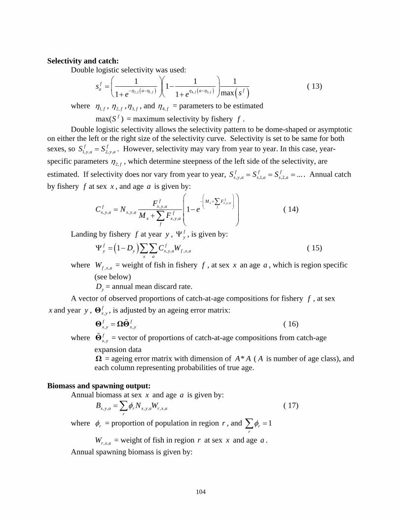
104

Selectivity and catch: Double logistic selectivity was used:

( ) ( ) ( )2, 1, 4, 3,

1 1 11max1 1f f f f

fa fa a

sse eη η η η− − −

⎛ ⎞⎛ ⎞= −⎜ ⎟⎜ ⎟

+ +⎝ ⎠⎝ ⎠ ( 13)

where 1, fη , 2, fη , 3, fη , and 4, fη = parameters to be estimated

max( )fS = maximum selectivity by fishery f . Double logistic selectivity allows the selectivity pattern to be dome-shaped or asymptotic on either the left or the right size of the selectivity curve. Selectivity is set to be same for both sexes, so 1, , 2, ,

f fy a y aS S= . However, selectivity may vary from year to year. In this case, year-

specific parameters 2, fη , which determine steepness of the left side of the selectivity, are

estimated. If selectivity does nor vary from year to year, , , ,1, ,2, ...f f fs y a s a s aS S S= = = . Annual catch

by fishery f at sex x , and age a is given by:

, ,

, ,, , , ,

, ,

1f

x x y af

f M Fx y af

x y a x y a fx x y a

f

FC N e

M F

⎛ ⎞⎜ ⎟− +⎜ ⎟⎝ ⎠

⎛ ⎞∑⎜ ⎟= −⎜ ⎟+ ⎜ ⎟⎝ ⎠

∑ ( 14)

Landing by fishery f at year y , fyΨ , is given by:

( ) , , , ,1f fy y x y a f x a

x aD C WΨ = − ∑∑ ( 15)

where , ,f x aW = weight of fish in fishery f , at sex x an age a , which is region specific (see below)

yD = annual mean discard rate. A vector of observed proportions of catch-at-age compositions for fishery f , at sex

x and year y , ,fx yΘ , is adjusted by an ageing error matrix:

, ,f fx y x y=Θ ΩΘ% ( 16)

where ,fx yΘ% = vector of proportions of catch-at-age compositions from catch-age

expansion data Ω = ageing error matrix with dimension of *A A ( A is number of age class), and

each column representing probabilities of true age. Biomass and spawning output: Annual biomass at sex x and age a is given by:

, , , , , ,x y a r x y a r x ar

B N Wφ= ∑ ( 17)

where rφ = proportion of population in region r , and 1rr

φ =∑

, ,r x aW = weight of fish in region r at sex x and age a . Annual spawning biomass is given by:

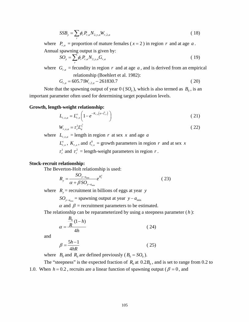
105

, 2, , ,2,y r r a y a r ar

SSB P N Wφ= ∑ ( 18)

where ,r aP = proportion of mature females ( 2x = ) in region r and at age a . Annual spawning output is given by:

, 2, , ,y r r a y a r ar

SO P N Gφ= ∑ ( 19)

where ,r aG = fecundity in region r and at age a , and is derived from an empirical relationship (Boehlert et al. 1982):

, ,2,605.71 261830.7r a r aG W= − ( 20) Note that the spawning output of year 0 ( 0SO ), which is also termed as 0B , is an important parameter often used for determining target population levels. Growth, length-weight relationship:

( )0, ,

, , , 1 r x r xK a tr x a r xL L e− −∞ ⎛ ⎞= −⎜ ⎟

⎝ ⎠ ( 21)

21

, ,r

r x a r aW Lττ= ( 22) where , ,r x aL = length in region r at sex x and age a

,r xL∞ , ,r xK , and 0,r xt = growth parameters in region r and at sex x

1rτ and 2

rτ = length-weight parameters in region r . Stock-recruit relationship:

The Beverton-Holt relationship is used: min

min

yRy ay

y a

SOR e

SOδ

α β−

−

=+

( 23)

where yR = recruitment in billions of eggs at year y

miny aSO − = spawning output at year miny a− α and β = recruitment parameters to be estimated.

The relationship can be reparameterized by using a steepness parameter ( h ):

0 (1 )

4

B hR

hα

−= ( 24)

and

5 14hhR

β −= ( 25)

where 0B and 0R are defined previously ( 0 0B SO= ). The “steepness” is the expected fraction of 0R at 00.2B , and is set to range from 0.2 to 1.0. When 0.2h = , recruits are a linear function of spawning output ( 0β = , and

106

min

1 yRy y aR SO e

δ

α −= ). When 1h = , recruits are constant and independent of spawning output

( 0α = , and 1 yRyR e

δ

β= ).

Abundance index:

The abundance index ( I ) for each fishery or survey ( i ) has the following relationship: i i fI q NS= ( 26)

where iq = catchability coefficient for fishery or survey i N = population abundance fS = selectivity of fishery or survey f that is associated with i .

A power transformation could also be used to transform index or abundance. If it is used to transform index:

Pi i fI q NS= ( 27)

where P = power parameter for index i . Likelihood components: Total likelihood is the sum of all individual likelihood from catch-at-age compositions, fishery landings, and CPUE indexes from surveys and commercial catch data. Where there are missing observed values, the likelihood values are set to zeros. The total negative logarithm of the likelihood, which will be minimized during the parameter estimation, is given by: log( ) i i

iL Lλ− = ∑ ( 28)

where iL = likelihood value for component i iλ = weighting factor for component i . Catch-at-age composition:

, ,1 , ,

, ,

ˆlog

fx y af f

y x y a ff y x a x y a

L nθ

θθ

⎛ ⎞= − ⎜ ⎟⎜ ⎟

⎝ ⎠∑∑ ∑∑ ( 29)

where θ and θ = observed and estimated proportions of catch-at-age compositions by fishery f at sex x , year y , and age a

fyn = sampled trips in fishery f and year y .

Landings:

( ) ( )

( )( )

2

2 2

ˆlog loglog

2

f fy y

ff f

L σσ

Ψ

Ψ

⎧ ⎫⎡ ⎤Ψ − Ψ⎪ ⎪⎣ ⎦= +⎨ ⎬⎪ ⎪⎩ ⎭

∑ ( 30)

where fyΨ and ˆ f

yΨ = observed and estimated landings by fishery f in year y

107

fσ Ψ = standard error for ( )log fyΨ which is set to be small (0.05) based on

the assumption of small observation errors of catch data.

Recruitment: Recruitment residuals are assumed to have no autocorrelations:

2

3 0.5 log( )yR

y R

RL

δ

σσ

⎡ ⎤⎛ ⎞⎢ ⎥= −⎜ ⎟⎜ ⎟⎢ ⎥⎝ ⎠⎣ ⎦

∑ ( 31)

Survey and CPUE indexes:

( ) ( )

( )( )

2

, ,

4 9 2

ˆlog loglog

2

j y j y IjIj j

I IL σ

σ−

⎧ ⎫⎡ ⎤−⎪ ⎪⎣ ⎦= +⎨ ⎬⎪ ⎪⎩ ⎭

∑ ( 32)

where ,j yI and ,ˆ

j yI = observed and estimated index from series j and year y

Ijσ = standard error for ( ),log j yI .

108

Appendix D: Input data for widow rockfish stock assessment base model. # **************************************************************** # Widow rockfish stock assessment data # Xi He # National Marine Fisheries Service # Southwest Fisheries Science Center # Santa Cruz Lab # xi.he@noaa.gov # July 2005 # Filename: wdwmaster.dat # **************************************************************** # number of region 2 # number of fishery 4 # number of sex 2 # number of observed indexes 6 # Starting and ending year of the model 1958 2004 47 # Recruitment age and total number of age bins 3 18 # Vector of ages for age bins 3 4 5 6 7 8 9 10 11 12 13 14 15 16 17 18 19 20 # number of likelihood components 9 # Natural mortality 0.125 0.125 # Discard rate (D value) by year (landing = catch * (1-D) ) 0.06 0.06 0.06 0.06 0.06 0.06 0.06 0.06 0.06 0.06 0.06 0.06 0.06 0.06 0.06 0.06 0.06 0.06 0.06 0.06 0.06 0.06 0.06 0.06 0.06 0.16 0.16 0.16 0.16 0.16 0.16 0.16 0.16 0.16 0.16 0.16 0.16 0.16 0.16 0.16 0.16 0.16 0.16 0.16 0.16 0.16 0.16 # Smoothed fraction of total landings in the north\ # fractions from 1968-77 was used in years before 1968, same as in 2000 assessment # foreign landings from Jean Rogers were not used to compute fractions before 1968 # new data 0.548 0.548 0.548 0.548 0.548 0.548 0.548 0.548 0.548 0.548 0.548 0.548 0.548 0.548 0.548 0.548 0.548 0.548 0.548 0.569 0.598 0.593 0.592 0.598 0.607 0.666 0.670 0.668 0.703 0.726 0.746 0.770 0.789 0.795 0.783 0.773 0.771 0.755 0.754 0.735 0.723 0.738 0.748 0.731 0.731 0.731 0.731 # Biological information # Growth parameters (Linf,K,t0 for male north, female north, male south, female south) # age 22 used for wgt of 20+ 44.00 50.54 41.50 47.55

109

0.18 0.14 0.25 0.20 -2.81 -2.68 -0.28 -0.17 # Length weight parameters (b and a for male and female) 0.01188 0.00545 3.06631 3.28781 # proportions of maturity of females # north 0.01 0.02 0.10 0.32 0.68 0.90 0.98 0.99 1.00 1.00 1.00 1.00 1.00 1.00 1.00 1.00 1.00 1.00 # south 0.13 0.21 0.64 0.90 0.90 1.00 1.00 1.00 1.00 1.00 1.00 1.00 1.00 1.00 1.00 1.00 1.00 1.00 # fecundity of females (millions of eggs) # north 0.0000 0.0000 0.0723 0.1526 0.2325 0.3102 0.3843 0.4540 0.5186 0.5780 0.6322 0.6812 0.7253 0.7648 0.8000 0.8313 0.8590 0.9241 # south 0.0050 0.0100 0.0300 0.0861 0.1788 0.2664 0.3466 0.4184 0.4813 0.5358 0.5824 0.6219 0.6552 0.6831 0.7064 0.7258 0.7419 0.7751 # index values 1968-1999 (-1 = no data) # NMFS Tiburon/Santa Cruz Lab midwater trawl index # data copied from Excel file "compare_time_series_with-without_stations.xls" sent by EJ 5-9-2004" # note that there were no estimates in 1992, 1996, and 1998 because of no positive catches # 1/2 of historical low estimates (value in 1994) were uesed in those years. # CVs were set very high. # only last 2 years data added, proportioan to old data from data sent by EJ 4-28-2004 -1.000000 -1.000000 -1.000000 -1.000000 -1.000000 -1.000000 -1.000000 -1.000000 -1.000000 -1.000000 -1.000000 -1.000000 -1.000000 -1.000000 -1.000000 -1.000000 -1.000000 -1.000000 -1.000000 -1.000000 -1.000000 -1.000000 -1.000000 -1.000000 -1.000000 -1.000000 4.456287 14.319479 0.152868 4.809881 3.757728 0.206186 0.230129 1.452406 0.067504 0.878655 0.135008 0.230438 0.067504 0.283063 0.067504 0.296648 0.287885 1.311048 6.561266 1.742240 2.379322 # Oregon bottom trawl index -1.00000 -1.00000 -1.00000 -1.00000 -1.00000 -1.00000 -1.00000 -1.00000 -1.00000 -1.00000 -1.00000 -1.00000 -1.00000 -1.00000 -1.00000 -1.00000 -1.00000 -1.00000 -1.00000 -1.00000 -1.00000 -1.00000 -1.00000 -1.00000 -1.00000 -1.00000 331.47 100.88 227.08 169.08 93.97 164.10 78.49 73.59 83.16 53.58 100.34 109.96 94.81 97.23 56.56 84.46 -1.00000 -1.00000 -1.00000 -1 -1 # Whiting bycatch index - foreign # 2005 new index - same as in 2003 but with STAR recom. and rescaled to mean -1.000000 -1.000000 -1.000000 -1.000000 -1.000000 -1.000000 -1.000000 -1.000000 -1.000000 -1.000000 -1.000000 -1.000000 -1.000000 -1.000000 -1.000000 -1.000000 -1.000000 -1.000000 -1.000000 0.770 1.205 0.703 1.993 0.728 0.243 -1.000000 2.937 0.407 1.111 0.390 0.513 -1.000000 -1.000000 -1.000000 -1.000000 -1.000000 -1.000000 -1.000000 -1.000000 -1.000000 -1.000000 -1.000000 -1.000000 -1.000000 -1.000000 -1.000000 -1.000000 # Whiting bycatch index - joint venture (JV) # 2005 new index - same as in 2003 but with STAR recom. and rescaled to mean -1.000000 -1.000000 -1.000000 -1.000000 -1.000000

110

-1.000000 -1.000000 -1.000000 -1.000000 -1.000000 -1.000000 -1.000000 -1.000000 -1.000000 -1.000000 -1.000000 -1.000000 -1.000000 -1.000000 -1.000000 -1.000000 -1.000000 -1.000000 -1.000000 -1.000000 2.889 -1.000000 0.776 0.823 0.320 0.659 0.824 0.710 -1.000000 -1.000000 -1.000000 -1.000000 -1.000000 -1.000000 -1.000000 -1.000000 -1.000000 -1.000000 -1.000000 -1.000000 -1 -1 # Whiting bycatch index - domestic # 2005 new index - same as in 2003 but with STAR recom. and rescaled to mean -1.000000 -1.000000 -1.000000 -1.000000 -1.000000 -1.000000 -1.000000 -1.000000 -1.000000 -1.000000 -1.000000 -1.000000 -1.000000 -1.000000 -1.000000 -1.000000 -1.000000 -1.000000 -1.000000 -1.000000 -1.000000 -1.000000 -1.000000 -1.000000 -1.000000 -1.000000 -1.000000 -1.000000 -1.000000 -1.000000 -1.000000 -1.000000 -1.000000 1.2642 0.7812 0.8009 1.4653 0.4546 1.0182 0.8855 1.3301 -1.000000 -1.000000 -1.000000 -1.000000 -1.000000 -1.000000 # Triennual Survey index # July 7 2005 results from John, base model 1 -1 -1 -1 -1 -1 -1 -1 -1 -1 -1 -1 -1 -1 -1 -1 -1 -1 -1 -1 0.506 -1 -1 0.382 -1 -1 0.565 -1 -1 0.353 -1 -1 0.390 -1 -1 0.461 -1 -1 0.305 -1 -1 0.692 -1 -1 0.112 -1 -1 0.126 # cv for each index # cv for NMFS Tiburon/Santa Cruz Lab midwater trawl index -1.0000 -1.0000 -1.0000 -1.0000 -1.0000 -1.0000 -1.0000 -1.0000 -1.0000 -1.0000 -1.0000 -1.0000 -1.0000 -1.0000 -1.0000 -1.0000 -1.0000 -1.0000 -1.0000 -1.0000 -1.0000 -1.0000 -1.0000 -1.0000 -1.0000 -1.0000 0.4346 0.4897 0.5020 0.2485 0.2869 0.4164 0.4297 0.3197 2.0000 0.2849 0.4880 0.4941 2.0000 0.4214 2.0000 0.5001 0.3657 0.2721 0.3156 0.5 0.5 # cv for Oregon bottom trawl index -1 -1 -1 -1 -1 -1 -1 -1 -1 -1 -1 -1 -1 -1 -1 -1 -1 -1 -1 -1 -1 -1 -1 -1 -1 -1.0 0.2121 0.1875 0.2928 0.2730 0.2897 0.1749 0.1348 0.1275 0.1179 0.1314 0.1128 0.1387 0.1357 0.1502 0.1718 0.1684 -1.0 -1.0 -1.0 -1 -1 # cv for Whiting bycatch index - foreign # 2005 new index - same as in 2003 but with STAR recom. and rescaled to mean -1 -1 -1 -1 -1 -1 -1 -1 -1 -1 -1 -1 -1 -1 -1 -1 -1 -1 -1 0.1153162 0.1118053 0.1186495 0.1311275 0.1257054 0.2466747 -1 0.1253805 0.1074312 0.1026710 0.0880962

111

0.1243402 -1 -1 -1 -1 -1 -1 -1 -1 -1 -1 -1 -1 -1 -1 -1 -1 -1 -1 # cv for Whiting bycatch index - joint venture (JV) # 2005 new index - same as in 2003 but with STAR recom. and rescaled to mean -1 -1 -1 -1 -1 -1 -1 -1 -1 -1 -1 -1 -1 -1 -1 -1 -1 -1 -1 -1 -1 -1 -1 -1 -1 0.12015916 -1 0.11650305 0.08088591 0.08748436 0.07741054 0.06352467 0.07400396 -1 -1 -1 -1 -1 -1 -1 -1 -1 -1 -1 -1 -1 -1 # cv for Whiting bycatch index - domestic # 2005 new index - same as in 2003 but with STAR recom. and rescaled to mean -1 -1 -1 -1 -1 -1 -1 -1 -1 -1 -1 -1 -1 -1 -1 -1 -1 -1 -1 -1 -1 -1 -1 -1 -1 -1 -1 -1 -1 -1 -1 -1 -1 0.1251 0.1251 0.1038 0.0685 0.1057 0.0824 0.0767 0.0786 -1 -1 -1 -1 -1 -1 # Triennual Survey CV -1 -1 -1 -1 -1 -1 -1 -1 -1 -1 -1 -1 -1 -1 -1 -1 -1 -1 -1 0.1647139 -1 -1 0.17362109 -1 -1 0.20646497 -1 -1 0.13429315 -1 -1 0.20142058 -1 -1 0.17819659 -1 -1 0.1330084 -1 -1 0.24706085 -1 -1 0.04130032 -1 -1 0.3 # landings, data copied from "AllLanding for model.txt" # VAL-COL Fishery landings -1.0 -1.0 -1.0 -1.0 -1.0 -1.0 -1.0 -1.0 3670.0 3900.0 1693.0 356.0 554.0 701.0 410.0 617.0 293.0 454.0 948.0 1318.0 605.0 966.0 16190.0 21779.3 14802.4 3222.4 1450.4 1537.0 2559.1 3722.0 3078.1 3378.3 2240.7 1176.2 946.5 1746.9 1074.4 1087.3 965.1 1016.2 563.1 525.4 379.7 302.4 65.1 15.5 30.0 # OR midwater trwal fishery landings -1.0 -1.0 -1.0 -1.0 -1.0 -1.0 -1.0 -1.0 -1.0 -1.0 -1.0 -1.0 -1.0 -1.0 -1.0 -1.0 -1.0 -1.0 -1.0 -1.0 -1.0 -1.0 -1.0 -1.0 -1.0 1452.0 3567.6 3185.0 2976.9 4984.8 4101.6 4870.9 3234.8 1845.5 1149.4 1754.8 1678.4 1394.2 1463.6 1523.5 758.3 1721.0 2276.1 966.0 154.6 7.6 12.4 # OR bottom trwal fishery landings

112

-1.0 -1.0 -1.0 -1.0 -1.0 -1.0 -1.0 -1.0 -1.0 -1.0 -1.0 -1.0 -1.0 -1.0 -1.0 -1.0 -1.0 -1.0 -1.0 -1.0 -1.0 -1.0 -1.0 -1.0 -1.0 1487.6 1334.2 870.8 1170.7 1169.3 1121.0 1970.9 2167.5 1940.1 2624.3 3386.2 2382.5 2277.7 2114.5 2244.7 1329.7 794.0 16.3 38.9 5.6 0.2 2.4 # EUR-CON fishery landings -1.0 -1.0 -1.0 -1.0 -1.0 -1.0 -1.0 -1.0 96.0 249.0 336.0 21.0 1.0 1.0 13.0 207.0 280.0 358.0 412.0 883.0 502.0 2326.0 5666.0 5227.3 11244.8 4324.7 3506.0 3570.2 2800.2 3035.1 2183.0 2266.0 2579.2 1369.2 1330.6 1347.4 1248.4 1943.8 1529.0 1707.4 1303.8 902.3 1140.9 504.9 51.1 5.1 27.8 # Age compositions from four fisheries # VAN-COL Fishery, data copied from "WAAge5.txt" # number of years of age comps 25 # years of age comps 1980 1981 1982 1983 1984 1985 1986 1987 1988 1989 1990 1991 1992 1993 1994 1995 1996 1997 1998 1999 2000 2001 2002 2003 2004 # number of sampled trips, data copied from "nSample_trip.txt" # next line: real number of trips # 18 31 40 25 22 16 27 36 20 30 41 35 31 34 28 33 25 29 22 29 21 10 12 5 19 # next line: fitted effective sample sizes # 100 174 223 140 121 90 151 202 111 167 230 197 174 190 156 185 140 162 121 162 116 55 67 28 106 # Dont change formats of next 2 lines (read by effective sample size programs) # VAN-COL Fishery new sample counts 100 174 223 140 121 90 151 202 111 167 230 197 174 190 156 185 140 162 121 162 116 55 67 28 106 # male age comps 0.000000 0.000000 0.009363 0.021512 0.020342 0.055539 0.095547 0.110577 0.046018 0.029204 0.011890 0.013060 0.005852 0.004096 0.002341 0.002341 0.001170 0.002926 0.000444 0.006609 0.024435 0.063737 0.045524 0.024041 0.047744 0.087771 0.067569 0.047083 0.025763 0.017104 0.011660 0.005331 0.004276 0.003388 0.002887 0.008502 0.000155 0.008491 0.030499 0.084375 0.030692 0.044964 0.020568 0.021494 0.032650 0.071686 0.044941 0.034309 0.034855 0.021097 0.014068 0.008806 0.005466 0.016884 0.000000 0.007569 0.153715 0.113485 0.028422 0.017474 0.014261 0.013099 0.013587 0.018363 0.020143 0.014780 0.015317 0.008811 0.006339 0.006692 0.005666 0.019890 0.000000 0.003350 0.053703 0.161029 0.083344 0.033419 0.013850 0.004392 0.005597 0.006802 0.007517 0.012931 0.012788 0.010684 0.006802 0.007681 0.007681 0.028558 0.000000 0.008297 0.074816 0.080420 0.124782 0.066450 0.021605 0.009465 0.003556 0.005909 0.005317 0.006053 0.005460 0.002658 0.005909 0.004724 0.002514 0.028344 0.000000 0.007004 0.060179 0.173641 0.075174 0.048950 0.014384 0.005971 0.005285 0.005216 0.003465 0.003122 0.004632 0.006073 0.003224 0.002297 0.001542 0.029481 0.000000 0.006265 0.024049 0.120012 0.194208 0.046191 0.012870 0.008530 0.002837 0.004189 0.005540 0.004207 0.003007 0.004055 0.003750 0.002112 0.001504 0.011251 0.000000 0.000000 0.014864 0.060143 0.136868 0.198862 0.034969 0.013274 0.004554 0.002449 0.000859 0.002620 0.003136 0.000859 0.000172 0.000515 0.000687 0.014043 0.000000 0.002563 0.017604 0.093364 0.094971 0.157016 0.087374 0.009204 0.003722 0.001158 0.000000 0.001282 0.000232 0.000927 0.000232 0.000463 0.001513 0.008464 0.000000 0.000463 0.025076 0.077338 0.152505 0.068068 0.097415 0.029967 0.011481 0.004530 0.000978 0.000463 0.000000 0.000463 0.000515 0.000978 0.001030 0.007465 0.000000 0.001239 0.010046 0.061669 0.114105 0.107253 0.073670 0.043532 0.049591 0.010278 0.003949 0.002903 0.001665 0.000619 0.004045 0.001142 0.001142 0.018292 0.000000 0.002617 0.019543 0.030901 0.071545 0.077261 0.081928 0.048736 0.051520 0.029444 0.019793 0.007934 0.004909 0.002700 0.001717 0.000000 0.000900 0.011618 0.000185 0.000185 0.016425 0.058431 0.050747 0.063019 0.056698 0.035194 0.029057 0.030791 0.022921 0.020327 0.012207 0.006507 0.005330 0.004338 0.001984 0.013384

113

0.000000 0.001331 0.010582 0.041369 0.086868 0.057047 0.045363 0.037112 0.028125 0.022800 0.025962 0.016475 0.012947 0.011150 0.004926 0.003595 0.002696 0.017475 0.000691 0.010249 0.030940 0.056238 0.096199 0.099808 0.063916 0.028599 0.030595 0.018657 0.014971 0.023609 0.010403 0.007409 0.006142 0.007217 0.002457 0.011977 0.000825 0.012122 0.059141 0.111858 0.104217 0.057559 0.032922 0.018325 0.013448 0.010364 0.007925 0.006347 0.007925 0.002367 0.003156 0.003192 0.002403 0.007925 0.000000 0.002832 0.036764 0.148943 0.129095 0.049633 0.015218 0.009554 0.006238 0.006811 0.006631 0.008137 0.001326 0.003316 0.002653 0.000663 0.000753 0.003979 0.000000 0.001088 0.014273 0.042774 0.145687 0.109655 0.039772 0.014534 0.007136 0.008529 0.007702 0.003307 0.002481 0.002481 0.006615 0.000827 0.000000 0.005788 0.000000 0.001831 0.011040 0.040933 0.080731 0.107025 0.081930 0.041423 0.022625 0.009912 0.009801 0.009154 0.004577 0.005224 0.003662 0.004577 0.001831 0.005224 0.000000 0.000000 0.004588 0.057879 0.112760 0.071044 0.073473 0.072574 0.038416 0.012596 0.012326 0.005248 0.002099 0.009117 0.006298 0.003149 0.002099 0.005248 0.000000 0.000000 0.004115 0.051421 0.125572 0.084227 0.061767 0.053575 0.037152 0.039345 0.033114 0.008307 0.016538 0.006231 0.006192 0.006231 0.002077 0.006231 0.000000 0.001570 0.020404 0.025113 0.056503 0.097311 0.062781 0.051795 0.023543 0.025113 0.010987 0.014126 0.001570 0.001570 0.004709 0.001570 0.001570 0.003139 0.000000 0.003354 0.060372 0.080496 0.083850 0.060372 0.016770 0.003354 0.000000 0.000000 0.000000 0.003354 0.000000 0.000000 0.000000 0.000000 0.000000 0.000000 0.000000 0.000000 0.034579 0.102089 0.044458 0.039518 0.027992 0.009880 0.013173 0.004940 0.003293 0.004940 0.003293 0.001647 0.103171 0.003293 0.000000 0.106464 # female age comps 0.000000 0.000000 0.009150 0.018485 0.013561 0.025721 0.087940 0.141807 0.084614 0.062747 0.034713 0.017742 0.021253 0.018513 0.005267 0.007023 0.006437 0.013246 0.000000 0.007494 0.017214 0.046582 0.043915 0.020375 0.020432 0.062351 0.078447 0.071291 0.037376 0.028320 0.018543 0.010161 0.005388 0.005778 0.005167 0.027296 0.000311 0.007559 0.018373 0.059590 0.028839 0.041575 0.018823 0.014979 0.014679 0.049251 0.039979 0.040337 0.032736 0.032280 0.016563 0.015107 0.005932 0.037088 0.000000 0.005567 0.153308 0.113974 0.040329 0.020551 0.009182 0.013519 0.013334 0.016294 0.029275 0.022800 0.021589 0.013149 0.010306 0.006877 0.004523 0.027811 0.001062 0.001941 0.044000 0.152020 0.075377 0.025555 0.018160 0.005270 0.006496 0.007007 0.011378 0.016832 0.025126 0.023716 0.020100 0.010888 0.013543 0.081403 0.000000 0.008297 0.070811 0.081461 0.117263 0.057561 0.027515 0.008568 0.006951 0.005317 0.007526 0.005460 0.012394 0.009592 0.010921 0.007221 0.007526 0.099337 0.000000 0.002024 0.053314 0.177620 0.091239 0.069749 0.020146 0.013248 0.003947 0.006967 0.007652 0.006142 0.008884 0.008402 0.007717 0.009157 0.003497 0.060653 0.000152 0.004475 0.013899 0.095086 0.224047 0.056797 0.036973 0.025570 0.009424 0.006740 0.003750 0.001960 0.007062 0.007536 0.004833 0.007518 0.004225 0.035374 0.000000 0.002449 0.007346 0.056149 0.150873 0.206253 0.035268 0.017268 0.012072 0.008205 0.002964 0.000343 0.002620 0.000515 0.000343 0.000859 0.000172 0.007428 0.000000 0.002563 0.007104 0.075898 0.092900 0.183621 0.104391 0.008972 0.009790 0.005822 0.000695 0.001050 0.001050 0.001513 0.000000 0.000927 0.003613 0.020000 0.000000 0.001442 0.027599 0.062045 0.115589 0.077798 0.119347 0.059061 0.012203 0.005509 0.002523 0.002935 0.000463 0.001030 0.002471 0.000978 0.000927 0.029344 0.000000 0.000000 0.003852 0.054294 0.084316 0.099026 0.065618 0.056733 0.053597 0.010801 0.009330 0.004665 0.004142 0.002478 0.000619 0.003000 0.002381 0.040009 0.000000 0.003025 0.023468 0.025342 0.055352 0.091347 0.081863 0.056670 0.069345 0.045878 0.029852 0.011692 0.007850 0.004417 0.000900 0.003600 0.002125 0.024210 0.000000 0.000992 0.008240 0.059488 0.037733 0.068088 0.069636 0.054083 0.049865 0.084602 0.047576 0.029668 0.015358 0.008851 0.002910 0.004523 0.001918 0.028742 0.003527 0.002662 0.013346 0.046762 0.073879 0.067858 0.043795 0.054384 0.041437 0.043268 0.052121 0.034747 0.024631 0.016042 0.012947 0.007589 0.004426 0.030753 0.000691 0.009366 0.032054 0.050326 0.077658 0.081612 0.055470 0.036814 0.023493 0.027217 0.017198 0.020537 0.009674 0.006871 0.010749 0.004760 0.001574 0.013858 0.000000 0.001578 0.068428 0.112111 0.107589 0.064339 0.053686 0.023920 0.014381 0.018253 0.013448 0.011117 0.017428 0.004770 0.003945 0.001578 0.002403 0.019006 0.000000 0.000663 0.028716 0.167241 0.141840 0.052825 0.033179 0.023569 0.016848 0.017995 0.017331 0.010037 0.007294 0.010610 0.005395 0.001989 0.002653 0.029268 0.000000 0.001088 0.012053 0.047736 0.165172 0.153429 0.046648 0.020322 0.022758 0.023063 0.019539 0.021454 0.014273 0.004395 0.011271 0.004656 0.002481 0.017014 0.000000 0.001239 0.012224 0.046000 0.066841 0.126525 0.104823 0.052952 0.032860 0.022838 0.015081 0.013195 0.014378 0.008562 0.005816 0.011309 0.005493 0.018364 0.000000 0.000000 0.001769 0.053442 0.088260 0.097226 0.076924 0.069246 0.046094 0.021383 0.009837 0.009447 0.006298 0.006298 0.006298 0.009447 0.002099 0.007018 0.000000 0.000000 0.002077 0.024653 0.053421 0.090227 0.057421 0.014346 0.031076 0.024884 0.047768 0.035268 0.016615 0.018692 0.004154 0.006192 0.008307 0.022807 0.000000 0.001570 0.023543 0.025113 0.026682 0.102020 0.097311 0.042377 0.043947 0.032960 0.028252 0.025113 0.021973 0.009417 0.001570 0.010987 0.004709 0.020404

114

0.003354 0.013416 0.100620 0.053664 0.046956 0.057018 0.040248 0.010062 0.026832 0.006708 0.006708 0.006708 0.003354 0.003354 0.000000 0.000000 0.003354 0.003354 0.000000 0.001647 0.031285 0.123495 0.054338 0.060924 0.067510 0.037872 0.031285 0.016466 0.019759 0.011526 0.006586 0.001647 0.001647 0.001647 0.013173 0.016466 # OR Midwater Trawl Fishery # note that there are no age samples in 2003, so agecomp=(-1) for 2003, number of trip for 2003 is set to (-1) # number of years of age comps 21 # years of age comps 1984 1985 1986 1987 1988 1989 1990 1991 1992 1993 1994 1995 1996 1997 1998 1999 2000 2001 2002 2003 2004 # next line: real number of trips # 32 53 56 68 39 65 61 59 43 50 22 30 32 47 41 62 55 39 17 -1 4 # next line: fitted effective sample sizes # 108 179 189 228 131 219 206 199 145 169 74 102 108 158 140 209 185 131 56 -1 13 # Dont change formats of next 2 lines (read by effective sample size programs) # OR Midwater Trawl Fishery new sample counts 108 179 189 228 131 219 206 199 145 169 74 102 108 158 140 209 185 131 56 -1 13 # male age comps 0.000000 0.001319 0.017593 0.173774 0.112637 0.008768 0.019432 0.006853 0.008680 0.007585 0.015521 0.022620 0.001850 0.007780 0.003536 0.001885 0.000799 0.011921 0.000000 0.002119 0.066729 0.069127 0.223896 0.065433 0.007443 0.005645 0.002895 0.000000 0.001651 0.004627 0.012730 0.002508 0.002202 0.000000 0.000000 0.009610 0.000000 0.000000 0.005477 0.104213 0.073568 0.195207 0.059686 0.004991 0.005093 0.003767 0.000000 0.000447 0.001135 0.012793 0.003980 0.002753 0.001404 0.007583 0.000000 0.000000 0.014196 0.125268 0.217513 0.074011 0.041905 0.022240 0.002491 0.003416 0.002991 0.000421 0.000236 0.001845 0.003615 0.000000 0.001370 0.003318 0.000463 0.001134 0.013597 0.076953 0.244116 0.129001 0.033834 0.020208 0.007744 0.000000 0.001440 0.000441 0.000851 0.000000 0.002627 0.002040 0.000000 0.003489 0.000000 0.005576 0.018629 0.054351 0.121196 0.199054 0.068330 0.016187 0.009606 0.002806 0.000780 0.000588 0.000503 0.000680 0.002170 0.002169 0.003530 0.005834 0.000000 0.003259 0.027658 0.029435 0.056774 0.099210 0.133459 0.067073 0.032413 0.015428 0.007388 0.003535 0.000000 0.000956 0.000000 0.001783 0.000000 0.004200 0.000000 0.000000 0.007865 0.064272 0.099804 0.106824 0.065076 0.089038 0.038706 0.009747 0.011371 0.003156 0.002466 0.001678 0.001335 0.000000 0.000553 0.009008 0.000000 0.000000 0.035945 0.039720 0.087052 0.083027 0.080416 0.041211 0.085709 0.030049 0.021923 0.013500 0.002018 0.004160 0.000000 0.000000 0.001193 0.013024 0.000000 0.000000 0.016302 0.070921 0.055203 0.081487 0.049299 0.038564 0.034325 0.059574 0.026062 0.017941 0.014803 0.006404 0.000000 0.003025 0.001142 0.010385 0.000060 0.001656 0.008803 0.075885 0.155556 0.079729 0.046850 0.041458 0.011685 0.019825 0.031305 0.000000 0.001604 0.005385 0.000000 0.000000 0.000000 0.009487 0.000031 0.004062 0.016837 0.024621 0.130919 0.094844 0.048282 0.043438 0.032006 0.022568 0.029549 0.006968 0.001389 0.000584 0.000199 0.005330 0.000099 0.001390 0.000000 0.008243 0.073067 0.092792 0.070761 0.065215 0.049392 0.033786 0.013582 0.008126 0.023971 0.009317 0.017184 0.008103 0.003180 0.000000 0.004503 0.005028 0.000000 0.002472 0.031114 0.240239 0.116098 0.042764 0.026053 0.026697 0.016128 0.013262 0.008786 0.003029 0.013826 0.012758 0.000238 0.000317 0.000627 0.002079 0.000000 0.000000 0.011590 0.081244 0.194209 0.111829 0.054206 0.014576 0.025467 0.014974 0.003056 0.007315 0.000585 0.000827 0.008645 0.002236 0.000510 0.004328 0.000000 0.001307 0.025490 0.038238 0.109048 0.181498 0.087210 0.021738 0.004939 0.005506 0.000349 0.000900 0.001168 0.000127 0.000704 0.000518 0.000027 0.002181 0.000000 0.000000 0.005109 0.032082 0.072429 0.085135 0.107367 0.083443 0.044698 0.030223 0.004426 0.006738 0.008699 0.002806 0.000456 0.000033 0.000014 0.000058 0.000000 0.000000 0.001242 0.018150 0.098439 0.099310 0.120418 0.061821 0.049969 0.041947 0.016620 0.005991 0.001932 0.003066 0.001511 0.001557 0.004046 0.003968 0.000000 0.008723 0.008813 0.043887 0.089952 0.148003 0.117899 0.033222 0.013022 0.008925 0.009604 0.006716 0.000000 0.008839 0.004705 0.000000 0.007456 0.001564 -1.000000 -1.000000 -1.000000 -1.000000 -1.000000 -1.000000 -1.000000 -1.000000 -1.000000 -1.000000 -1.000000 -1.000000 -1.000000 -1.000000 -1.000000 -1.000000 -1.000000 -1.000000 0.000000 0.080014 0.140150 0.202790 0.080660 0.026095 0.014545 0.001682 0.002243 0.001682 0.001121 0.001682 0.001121 0.000000 0.000000 0.000561 0.001121 0.000561 # female age comps 0.000000 0.001510 0.019934 0.162448 0.181347 0.014814 0.030019 0.006296 0.006676 0.003755 0.028175 0.060927 0.016433 0.008933 0.006848 0.005805 0.005883 0.017642 0.000000 0.000000 0.053076 0.066565 0.251723 0.085721 0.011142 0.010688 0.008649 0.000000 0.000528 0.007035 0.017174 0.001930 0.000732 0.001306 0.001919 0.005197

115

0.000000 0.000000 0.009632 0.136515 0.082265 0.167834 0.067183 0.004427 0.010719 0.004415 0.000000 0.000378 0.003940 0.016357 0.001389 0.002327 0.001567 0.008954 0.000000 0.001290 0.016675 0.112688 0.198001 0.080151 0.038100 0.020477 0.001549 0.004767 0.001785 0.000132 0.000917 0.001633 0.002851 0.001500 0.000435 0.002213 0.000984 0.004680 0.014524 0.076746 0.192350 0.099018 0.025664 0.016977 0.008845 0.004252 0.004467 0.000000 0.001045 0.000000 0.001373 0.004050 0.002694 0.004392 0.000000 0.004348 0.026249 0.036418 0.079465 0.197050 0.086376 0.023765 0.011445 0.005620 0.004468 0.001832 0.000000 0.000745 0.000509 0.001577 0.001323 0.006822 0.000000 0.000000 0.018125 0.033563 0.054101 0.079333 0.150790 0.103895 0.037364 0.021728 0.009049 0.002238 0.001919 0.000577 0.000840 0.000000 0.000000 0.003908 0.000000 0.000000 0.010207 0.061722 0.096026 0.060650 0.068546 0.098079 0.042946 0.013639 0.009989 0.004482 0.003192 0.000781 0.000484 0.000484 0.002413 0.015458 0.000000 0.000000 0.023080 0.029597 0.070216 0.075317 0.042247 0.063636 0.088798 0.031001 0.015295 0.006497 0.001193 0.001984 0.002030 0.002224 0.000000 0.007939 0.000000 0.000619 0.010235 0.067949 0.036055 0.079940 0.065430 0.035775 0.045776 0.067009 0.033835 0.023914 0.020267 0.010147 0.004298 0.005024 0.001773 0.006514 0.000000 0.000060 0.008346 0.048716 0.157869 0.064175 0.055961 0.041445 0.034903 0.024695 0.028568 0.014965 0.020718 0.004541 0.000000 0.000000 0.002325 0.003423 0.000000 0.004768 0.005481 0.030657 0.058610 0.087557 0.088895 0.056843 0.042520 0.038741 0.032444 0.046168 0.012590 0.007441 0.014045 0.001228 0.000153 0.008744 0.000000 0.007131 0.067434 0.059398 0.076746 0.079752 0.049421 0.023895 0.038792 0.016466 0.018451 0.023365 0.018283 0.005841 0.000700 0.000878 0.000572 0.026625 0.000000 0.002580 0.012439 0.169835 0.081572 0.038429 0.037679 0.017000 0.014256 0.011551 0.013032 0.013201 0.006873 0.016518 0.001471 0.002426 0.000000 0.004652 0.000000 0.000037 0.004497 0.036935 0.158466 0.091903 0.047566 0.030986 0.031988 0.014652 0.014922 0.012049 0.003880 0.001903 0.006640 0.000777 0.002699 0.004503 0.000000 0.000166 0.022686 0.036414 0.081014 0.185689 0.092911 0.040511 0.019957 0.008138 0.011300 0.006752 0.000919 0.007343 0.003825 0.000516 0.000007 0.000904 0.000000 0.000000 0.008677 0.031407 0.070586 0.097748 0.079331 0.090545 0.060205 0.026866 0.016246 0.007038 0.008829 0.003891 0.003141 0.001463 0.005690 0.004620 0.000000 0.000000 0.000000 0.012758 0.067117 0.066960 0.071267 0.068666 0.049195 0.060219 0.016257 0.009531 0.008203 0.008080 0.013686 0.008207 0.005712 0.004153 0.000000 0.002825 0.009167 0.017950 0.065404 0.114271 0.090580 0.082117 0.036436 0.033172 0.014684 0.004683 0.009396 0.000044 0.004637 0.000044 0.001564 0.001696 -1.000000 -1.000000 -1.000000 -1.000000 -1.000000 -1.000000 -1.000000 -1.000000 -1.000000 -1.000000 -1.000000 -1.000000 -1.000000 -1.000000 -1.000000 -1.000000 -1.000000 -1.000000 0.005417 0.110513 0.075197 0.151982 0.070732 0.022576 0.005871 0.000561 0.000561 0.000561 0.000000 0.000000 0.000000 0.000000 0.000000 0.000000 0.000000 0.000000 # OR Bottom Trawl Fishery # number of years of age comps 16 # years of age comps 1984 1985 1986 1987 1988 1989 1990 1991 1992 1993 1994 1995 1996 1997 1998 1999 # next line: real number of trips # 27 23 22 34 33 45 49 78 82 61 63 43 27 40 30 26 # next line: fitted effective sample sizes # 94 81 78 118 114 157 172 273 287 214 220 150 94 139 105 91 # Dont change formats of next 2 lines (read by effective sample size programs) # OR Bottom Trawl Fishery new sample counts 94 81 78 118 114 157 172 273 287 214 220 150 94 139 105 91 # male age comps 0.000000 0.002000 0.030445 0.189548 0.117081 0.016035 0.015324 0.003114 0.003439 0.001948 0.018194 0.013253 0.009686 0.007799 0.006124 0.002928 0.001011 0.009201 0.000000 0.002502 0.036013 0.074608 0.200140 0.051173 0.001874 0.004660 0.004952 0.000000 0.001042 0.008356 0.028493 0.000000 0.005334 0.003539 0.000143 0.007644 0.000000 0.002454 0.013907 0.200127 0.081379 0.084660 0.058424 0.002879 0.018185 0.005389 0.002106 0.000000 0.001445 0.017611 0.002031 0.001018 0.002843 0.015694 0.000000 0.000000 0.011118 0.109017 0.203522 0.070081 0.039469 0.015803 0.002859 0.002428 0.006852 0.000000 0.000000 0.005938 0.005288 0.001991 0.000000 0.007686 0.001871 0.011031 0.016633 0.079520 0.207515 0.102423 0.021828 0.011340 0.007407 0.003053 0.000490 0.000111 0.001142 0.000177 0.002442 0.003514 0.001270 0.006522 0.000000 0.008833 0.024646 0.049996 0.092063 0.174036 0.067810 0.031354 0.014894 0.008040 0.000000 0.006094 0.000196 0.000020 0.001275 0.000668 0.006091 0.006210 0.000000 0.003583 0.046610 0.044816 0.055997 0.068434 0.115960 0.057955 0.020822 0.019537 0.009585 0.004483 0.001307 0.002656 0.000000 0.000000 0.000000 0.011648 0.000000 0.000147 0.004189 0.070284 0.100833 0.070524 0.042126 0.076314 0.037653 0.009481 0.011792 0.003212 0.001068 0.003579 0.000182 0.000000 0.001193 0.011880

116

0.000000 0.000210 0.017104 0.021507 0.083738 0.072799 0.059036 0.034356 0.048167 0.017539 0.028795 0.015892 0.004209 0.004150 0.005980 0.001566 0.002672 0.017018 0.000000 0.000000 0.005855 0.035253 0.034549 0.088243 0.091091 0.046518 0.033369 0.054327 0.034564 0.022812 0.013524 0.004287 0.002129 0.003937 0.000464 0.016873 0.000000 0.003066 0.014275 0.056658 0.107092 0.068690 0.042280 0.016704 0.020763 0.028991 0.023737 0.008231 0.006195 0.004521 0.008745 0.002407 0.000000 0.010728 0.000000 0.002979 0.033648 0.108932 0.073740 0.135371 0.039055 0.044337 0.020910 0.017927 0.007067 0.012256 0.004705 0.005004 0.005162 0.000343 0.000000 0.002308 0.000000 0.001546 0.078624 0.082232 0.058865 0.058378 0.022296 0.017354 0.016860 0.020354 0.015502 0.002110 0.016646 0.004691 0.001983 0.010887 0.000918 0.007283 0.000000 0.006259 0.044095 0.229768 0.118118 0.047116 0.031456 0.020552 0.009284 0.017502 0.007340 0.006334 0.000686 0.005679 0.001947 0.000212 0.000000 0.003644 0.000000 0.000000 0.008048 0.051295 0.182533 0.115763 0.034581 0.021837 0.017118 0.020333 0.006225 0.009028 0.000040 0.001808 0.007220 0.000000 0.003032 0.007934 0.000000 0.004410 0.028185 0.065780 0.117624 0.177422 0.072072 0.027160 0.008664 0.000260 0.000000 0.007039 0.001389 0.000369 0.000145 0.000260 0.006664 0.002549 # female age comps 0.000000 0.000000 0.029195 0.150224 0.185481 0.027626 0.015787 0.011391 0.007173 0.004612 0.012420 0.029933 0.015032 0.008095 0.004631 0.005248 0.002645 0.043377 0.000442 0.000000 0.019813 0.048296 0.197706 0.126662 0.014812 0.017391 0.011417 0.000077 0.007641 0.022032 0.036411 0.010210 0.013434 0.002712 0.003324 0.037146 0.000000 0.001065 0.024770 0.106380 0.062244 0.095632 0.067643 0.006899 0.017635 0.013058 0.000257 0.000000 0.003719 0.043899 0.009910 0.006981 0.004659 0.025100 0.000000 0.001576 0.010234 0.117399 0.171871 0.063467 0.050337 0.029975 0.003580 0.003687 0.001518 0.003055 0.000272 0.004721 0.016566 0.013579 0.003342 0.022768 0.009606 0.014331 0.009403 0.077325 0.171310 0.103797 0.040625 0.026669 0.015156 0.010274 0.004624 0.005987 0.000830 0.002484 0.006360 0.010148 0.002759 0.010020 0.000000 0.001242 0.025824 0.027018 0.064659 0.144556 0.088917 0.041537 0.039946 0.014916 0.006732 0.006454 0.005084 0.003964 0.005380 0.003800 0.009658 0.018086 0.000000 0.000346 0.045983 0.035820 0.037131 0.067841 0.137383 0.107247 0.036003 0.017221 0.008657 0.004878 0.006605 0.002256 0.002494 0.001175 0.001334 0.024232 0.000000 0.000276 0.008559 0.057365 0.061216 0.065968 0.073102 0.107811 0.057796 0.032714 0.032940 0.007005 0.004608 0.004366 0.002101 0.000526 0.003298 0.035890 0.000000 0.000000 0.009753 0.008144 0.081541 0.088796 0.068771 0.057565 0.089954 0.047986 0.031772 0.019963 0.014438 0.004916 0.006446 0.001441 0.002506 0.031269 0.000000 0.000000 0.000299 0.025279 0.025262 0.075644 0.073311 0.044332 0.040169 0.066328 0.042838 0.028744 0.017316 0.020636 0.005716 0.008841 0.005620 0.031867 0.000000 0.002217 0.008820 0.042980 0.100462 0.063347 0.056897 0.063275 0.046037 0.026311 0.064738 0.028538 0.019849 0.012475 0.012450 0.006566 0.006008 0.015944 0.000000 0.004849 0.012570 0.037066 0.109137 0.084212 0.050834 0.038905 0.045410 0.025559 0.017455 0.024881 0.003947 0.002003 0.013073 0.001605 0.000000 0.014750 0.000097 0.007272 0.076010 0.101629 0.082023 0.086098 0.050735 0.028263 0.040649 0.032268 0.008394 0.004318 0.039893 0.000000 0.001771 0.010131 0.002891 0.011030 0.000000 0.008041 0.030840 0.103883 0.094444 0.030399 0.046719 0.030626 0.019097 0.014813 0.008142 0.013020 0.009741 0.016087 0.004702 0.000592 0.005036 0.013827 0.000000 0.000000 0.011607 0.047322 0.140566 0.110448 0.053762 0.024241 0.030259 0.017303 0.025682 0.013208 0.015729 0.002847 0.008011 0.001866 0.001373 0.008983 0.000000 0.000000 0.023360 0.057678 0.067752 0.146783 0.062621 0.042079 0.039373 0.008637 0.011882 0.006203 0.007617 0.002111 0.000000 0.001389 0.001141 0.001385 # EUR-CON Fishery # number of years of age comps 27 # years of age comps 1978 1979 1980 1981 1982 1983 1984 1985 1986 1987 1988 1989 1990 1991 1992 1993 1994 1995 1996 1997 1998 1999 2000 2001 2002 2003 2004 # number of trips sampled # next line: real number of trips # 7 11 26 44 149 189 169 175 154 135 127 170 155 95 55 22 28 11 35 61 37 31 17 7 14 3 7 # next line: fitted effective sample sizes # 5 7 16 27 93 117 104 109 96 83 78 105 97 59 35 14 18 7 22 38 23 19 11 5 9 2 5 # Dont change formats of next 2 lines (read by effective sample size programs) # EUR-CON Fishery new sample counts 5 7 16 27 93 117 104 109 96 83 78 105 97 59 35 14 18 7 22 38 23 19 11 5 9 2 5 # male age comps 0.000000 0.000000 0.000000 0.000167 0.038794 0.061910 0.113807 0.038798 0.047047 0.016198 0.015682 0.000104 0.015850 0.038590 0.000104 0.022908 0.000376 0.055254

117

0.000000 0.000000 0.000000 0.000000 0.011438 0.011620 0.048578 0.016812 0.020248 0.015707 0.009403 0.017248 0.001826 0.019215 0.010845 0.019730 0.000012 0.047583 0.000000 0.000000 0.001824 0.014065 0.002924 0.006643 0.039520 0.032312 0.050845 0.031275 0.025393 0.028792 0.009843 0.052786 0.003750 0.016236 0.004651 0.060013 0.000799 0.008361 0.010002 0.027066 0.025037 0.027711 0.025569 0.030219 0.042947 0.046706 0.023835 0.032838 0.015918 0.028874 0.012306 0.004370 0.013545 0.025365 0.000000 0.000106 0.043649 0.007338 0.036963 0.033485 0.030316 0.013544 0.043159 0.076267 0.035984 0.029549 0.019650 0.013771 0.016956 0.010418 0.008094 0.031557 0.000000 0.000086 0.022886 0.140348 0.031918 0.033224 0.012798 0.005381 0.007744 0.009472 0.019691 0.020034 0.012469 0.012446 0.004708 0.023251 0.002119 0.027271 0.000000 0.000000 0.022177 0.136865 0.144882 0.027534 0.035797 0.014452 0.013815 0.001723 0.010158 0.030363 0.014161 0.004130 0.005053 0.003807 0.004250 0.029903 0.000000 0.000227 0.008622 0.062244 0.162794 0.144850 0.012740 0.025432 0.011326 0.002269 0.002575 0.010161 0.021668 0.002268 0.004800 0.003061 0.003256 0.026758 0.000000 0.002672 0.041614 0.045810 0.082096 0.123917 0.129130 0.013757 0.021789 0.017389 0.001018 0.000893 0.008456 0.029102 0.005577 0.008659 0.003709 0.037843 0.001179 0.000152 0.054998 0.114196 0.043553 0.059667 0.090873 0.112021 0.019943 0.029954 0.021102 0.002845 0.000000 0.018666 0.014648 0.002809 0.011094 0.025925 0.000044 0.035380 0.000332 0.065560 0.060575 0.090206 0.060701 0.051129 0.034404 0.014184 0.008844 0.007881 0.003430 0.003586 0.006491 0.016135 0.001500 0.016273 0.000000 0.004922 0.108813 0.072992 0.077959 0.119011 0.046296 0.050071 0.019741 0.011676 0.020419 0.015728 0.008211 0.000000 0.000338 0.007197 0.005816 0.008951 0.000198 0.000005 0.045231 0.116161 0.029490 0.046574 0.037731 0.056019 0.029941 0.024640 0.016278 0.022979 0.019002 0.014258 0.003722 0.002474 0.008377 0.005882 0.000000 0.002436 0.015488 0.119032 0.119577 0.049449 0.037842 0.065086 0.022067 0.016393 0.020120 0.012377 0.001613 0.003541 0.003664 0.002594 0.002776 0.017436 0.000000 0.001110 0.011299 0.018839 0.138318 0.094889 0.037718 0.016739 0.044004 0.027766 0.021343 0.019358 0.011102 0.005458 0.016019 0.001048 0.001845 0.023196 0.000000 0.000000 0.084585 0.163306 0.095533 0.077734 0.009972 0.001732 0.009303 0.006881 0.010719 0.000920 0.020993 0.004707 0.001861 0.004059 0.000628 0.032682 0.001882 0.003574 0.007108 0.070279 0.148029 0.109588 0.064736 0.021235 0.023515 0.006816 0.007885 0.004744 0.006368 0.008510 0.000880 0.004805 0.000299 0.005238 0.000000 0.033490 0.039138 0.033789 0.056445 0.196870 0.044622 0.066035 0.057784 0.003157 0.028233 0.006769 0.020519 0.001013 0.004425 0.008088 0.000051 0.003038 0.003544 0.005653 0.046056 0.045052 0.066636 0.114331 0.117781 0.033128 0.026658 0.018426 0.015394 0.003008 0.024927 0.006853 0.002391 0.002031 0.008824 0.013330 0.000000 0.001634 0.008364 0.108288 0.040725 0.051077 0.052119 0.048417 0.049544 0.035874 0.026884 0.022934 0.012512 0.005025 0.004030 0.012426 0.006304 0.012199 0.000000 0.007713 0.081754 0.060620 0.092682 0.068982 0.053847 0.020544 0.045442 0.025031 0.018261 0.017733 0.005455 0.007462 0.009450 0.000313 0.000000 0.012849 0.000792 0.001303 0.018542 0.072137 0.059251 0.100602 0.069004 0.051386 0.026777 0.022079 0.029557 0.016272 0.006032 0.005804 0.005619 0.012011 0.004983 0.031026 0.000000 0.000000 0.003526 0.043905 0.060881 0.116213 0.055216 0.044377 0.027284 0.028240 0.009386 0.000345 0.002868 0.003058 0.008237 0.002356 0.002153 0.001940 0.000000 0.000172 0.000000 0.010409 0.072637 0.012072 0.064488 0.092402 0.034594 0.039625 0.032375 0.030079 0.041966 0.021130 0.004095 0.003259 0.000000 0.006689 0.000000 0.010264 0.001604 0.001684 0.015276 0.034963 0.043864 0.104166 0.028628 0.020809 0.097590 0.031715 0.060703 0.001604 0.030191 0.000000 0.032557 0.035925 0.000000 0.278761 0.013274 0.008850 0.008850 0.035398 0.039823 0.039823 0.000000 0.017699 0.000000 0.004425 0.013274 0.013274 0.000000 0.000000 0.000000 0.004425 0.000000 0.000000 0.023237 0.000000 0.014953 0.030713 0.053950 0.069711 0.038998 0.014953 0.047282 0.023237 0.007476 0.031522 0.038998 0.000000 0.007476 0.007476 # female age comps 0.000000 0.000000 0.000104 0.000000 0.123507 0.205950 0.041377 0.041169 0.018469 0.000000 0.061665 0.000208 0.000104 0.000000 0.000000 0.000208 0.000104 0.041545 0.000000 0.000000 0.000000 0.000000 0.028922 0.067305 0.158389 0.061886 0.061392 0.039940 0.075410 0.011394 0.019222 0.036234 0.011029 0.022589 0.029519 0.126505 0.000000 0.000000 0.000955 0.005649 0.003696 0.024150 0.063373 0.097604 0.097413 0.039497 0.051375 0.061888 0.017530 0.013496 0.029120 0.040354 0.006779 0.066250 0.000000 0.003318 0.004867 0.013777 0.035738 0.019389 0.024915 0.054715 0.072763 0.090769 0.026772 0.055740 0.045834 0.039020 0.025392 0.039669 0.010802 0.035053 0.000000 0.000304 0.032146 0.009081 0.035448 0.031095 0.024213 0.007839 0.036008 0.101644 0.051171 0.036445 0.034257 0.032311 0.023285 0.024933 0.016688 0.052326 0.000000 0.009591 0.075351 0.167412 0.047273 0.048111 0.015052 0.008820 0.002312 0.008036 0.037318 0.021821 0.012045 0.028244 0.019692 0.016134 0.025748 0.071191 0.000000 0.000000 0.025400 0.124378 0.113089 0.026752 0.029462 0.011598 0.007136 0.003342 0.019946 0.045211 0.009560 0.010595 0.006944 0.007132 0.010240 0.050144 0.000000 0.000151 0.001560 0.038649 0.152562 0.144097 0.019940 0.038756 0.006481 0.001962 0.002983 0.010131 0.022748 0.001717 0.006368 0.006675 0.009452 0.030716

118

0.000000 0.001094 0.032346 0.027042 0.073440 0.081848 0.100382 0.007086 0.021131 0.009354 0.004758 0.001774 0.001549 0.027713 0.003342 0.003768 0.003633 0.026310 0.001179 0.000098 0.047208 0.095361 0.021292 0.050757 0.050894 0.055412 0.011451 0.010172 0.004021 0.002340 0.000793 0.004487 0.002818 0.005991 0.000865 0.011236 0.000140 0.085843 0.037469 0.075957 0.071866 0.055259 0.032502 0.037143 0.021209 0.003896 0.014219 0.019743 0.004235 0.006851 0.003575 0.006002 0.008808 0.038628 0.000000 0.003411 0.081763 0.042605 0.042417 0.081496 0.053703 0.037811 0.021243 0.009702 0.007578 0.003805 0.006337 0.005543 0.000000 0.000650 0.001295 0.022498 0.000005 0.003187 0.050819 0.108911 0.056288 0.036766 0.088722 0.070834 0.037058 0.024351 0.009827 0.008493 0.006215 0.001197 0.003355 0.001205 0.002170 0.011633 0.000226 0.007123 0.008134 0.112901 0.128173 0.060714 0.030229 0.033110 0.023240 0.016982 0.013082 0.010959 0.008170 0.008172 0.006845 0.000731 0.001688 0.018028 0.000000 0.000232 0.015337 0.031121 0.108172 0.086481 0.039057 0.030308 0.037403 0.026187 0.025779 0.043862 0.015023 0.000488 0.001450 0.001391 0.005892 0.041767 0.000000 0.004208 0.033435 0.135163 0.123584 0.096949 0.036693 0.004437 0.001141 0.009519 0.007614 0.001330 0.000782 0.000971 0.001365 0.005160 0.005189 0.006846 0.001882 0.001724 0.022476 0.067422 0.161344 0.066366 0.050772 0.019637 0.025889 0.016917 0.015069 0.006851 0.009371 0.007548 0.006287 0.000228 0.001724 0.023001 0.000000 0.008129 0.009087 0.015496 0.050148 0.136555 0.049764 0.068335 0.023258 0.004577 0.007731 0.002032 0.005057 0.007653 0.000000 0.007704 0.000000 0.001013 0.005316 0.007498 0.039650 0.042831 0.041834 0.081434 0.058032 0.049604 0.037617 0.029501 0.010778 0.009947 0.012242 0.002580 0.001429 0.007214 0.004894 0.003579 0.000076 0.001013 0.007263 0.082973 0.037783 0.055790 0.052979 0.041542 0.064828 0.047760 0.030352 0.020260 0.004756 0.021095 0.006388 0.006955 0.005416 0.014417 0.000000 0.001686 0.053952 0.029427 0.075695 0.029682 0.045987 0.045308 0.052631 0.060361 0.028177 0.007907 0.009615 0.006146 0.006612 0.001982 0.003342 0.013353 0.000193 0.001612 0.010229 0.073635 0.045978 0.093642 0.041606 0.047047 0.038160 0.022148 0.021134 0.015287 0.014316 0.014162 0.003980 0.008607 0.001844 0.013246 0.000000 0.000000 0.006821 0.032812 0.098604 0.073335 0.075038 0.056790 0.039492 0.027416 0.059198 0.032557 0.032994 0.021127 0.002356 0.000562 0.023627 0.007284 0.000000 0.000000 0.000000 0.008190 0.060086 0.098599 0.036981 0.065238 0.063643 0.032407 0.037632 0.022603 0.020863 0.000945 0.012646 0.022527 0.033776 0.017871 0.000000 0.010264 0.001604 0.001403 0.031113 0.014715 0.038210 0.111904 0.048715 0.073654 0.004090 0.033960 0.030753 0.033399 0.003769 0.003368 0.000000 0.007538 0.013274 0.411504 0.039823 0.000000 0.000000 0.013274 0.004425 0.022124 0.004425 0.000000 0.000000 0.013274 0.000000 0.000000 0.000000 0.000000 0.000000 0.000000 0.000000 0.000000 0.014953 0.015761 0.014953 0.015761 0.038190 0.038190 0.068499 0.059810 0.066882 0.075571 0.014548 0.052738 0.046474 0.030713 0.007476 0.029501 # Ageing Error Matrix # row is true age, column is observed age (column sums to 1) 0.7620 0.1217 0.0006 0.0000 0.0000 0.0000 0.0000 0.0000 0.0000 0.0000 0.0000 0.0000 0.0000 0.0000 0.0000 0.0000 0.0000 0.0000 0.2315 0.7560 0.1244 0.0006 0.0000 0.0000 0.0000 0.0000 0.0000 0.0000 0.0000 0.0000 0.0000 0.0000 0.0000 0.0000 0.0000 0.0000 0.0065 0.1217 0.7500 0.1274 0.0007 0.0000 0.0000 0.0000 0.0000 0.0000 0.0000 0.0000 0.0000 0.0000 0.0000 0.0000 0.0000 0.0000 0.0000 0.0005 0.1244 0.7440 0.1303 0.0008 0.0000 0.0000 0.0000 0.0000 0.0000 0.0000 0.0000 0.0000 0.0000 0.0000 0.0000 0.0000 0.0000 0.0000 0.0006 0.1274 0.7380 0.1332 0.0009 0.0000 0.0000 0.0000 0.0000 0.0000 0.0000 0.0000 0.0000 0.0000 0.0000 0.0000 0.0000 0.0000 0.0000 0.0006 0.1303 0.7320 0.1361 0.0010 0.0000 0.0000 0.0000 0.0000 0.0000 0.0000 0.0000 0.0000 0.0000 0.0000 0.0000 0.0000 0.0000 0.0000 0.0007 0.1332 0.7260 0.1390 0.0011 0.0000 0.0000 0.0000 0.0000 0.0000 0.0000 0.0000 0.0000 0.0000 0.0000 0.0000 0.0000 0.0000 0.0000 0.0008 0.1361 0.7200 0.1419 0.0012 0.0000 0.0000 0.0000 0.0000 0.0000 0.0000 0.0000 0.0000 0.0000 0.0000 0.0000 0.0000 0.0000 0.0000 0.0009 0.1390 0.7140 0.1448 0.0014 0.0000 0.0000 0.0000 0.0000 0.0000 0.0000 0.0000 0.0000 0.0000 0.0000 0.0000 0.0000 0.0000 0.0000 0.0010 0.1419 0.7080 0.1476 0.0015 0.0000 0.0000 0.0000 0.0000 0.0000 0.0000 0.0000 0.0000 0.0000 0.0000 0.0000 0.0000 0.0000 0.0000 0.0011 0.1448 0.7020 0.1505 0.0017 0.0000 0.0000 0.0000 0.0000 0.0000 0.0000 0.0000 0.0000 0.0000 0.0000 0.0000 0.0000 0.0000 0.0000 0.0012 0.1476 0.6960 0.1533 0.0019 0.0000 0.0000 0.0000 0.0000 0.0000 0.0000 0.0000 0.0000 0.0000 0.0000 0.0000 0.0000 0.0000 0.0000 0.0014 0.1505 0.6900 0.1561 0.0020 0.0000 0.0000 0.0000 0.0000 0.0000 0.0000 0.0000 0.0000 0.0000 0.0000 0.0000 0.0000 0.0000 0.0000 0.0015 0.1533 0.6840 0.1590 0.0023 0.0000 0.0000

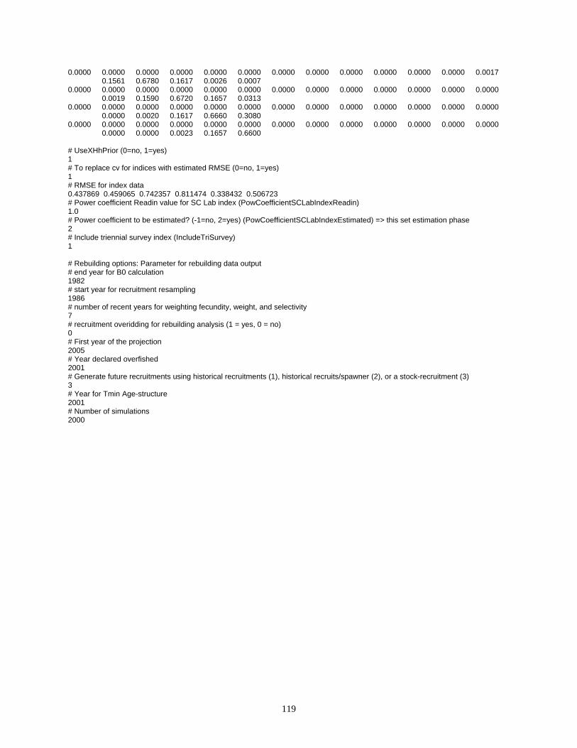
119

0.0000 0.0000 0.0000 0.0000 0.0000 0.0000 0.0000 0.0000 0.0000 0.0000 0.0000 0.0000 0.0017 0.1561 0.6780 0.1617 0.0026 0.0007 0.0000 0.0000 0.0000 0.0000 0.0000 0.0000 0.0000 0.0000 0.0000 0.0000 0.0000 0.0000 0.0000 0.0019 0.1590 0.6720 0.1657 0.0313 0.0000 0.0000 0.0000 0.0000 0.0000 0.0000 0.0000 0.0000 0.0000 0.0000 0.0000 0.0000 0.0000 0.0000 0.0020 0.1617 0.6660 0.3080 0.0000 0.0000 0.0000 0.0000 0.0000 0.0000 0.0000 0.0000 0.0000 0.0000 0.0000 0.0000 0.0000 0.0000 0.0000 0.0023 0.1657 0.6600 # UseXHhPrior (0=no, 1=yes) 1 # To replace cv for indices with estimated RMSE (0=no, 1=yes) 1 # RMSE for index data 0.437869 0.459065 0.742357 0.811474 0.338432 0.506723 # Power coefficient Readin value for SC Lab index (PowCoefficientSCLabIndexReadin) 1.0 # Power coefficient to be estimated? (-1=no, 2=yes) (PowCoefficientSCLabIndexEstimated) => this set estimation phase 2 # Include triennial survey index (IncludeTriSurvey) 1 # Rebuilding options: Parameter for rebuilding data output # end year for B0 calculation 1982 # start year for recruitment resampling 1986 # number of recent years for weighting fecundity, weight, and selectivity 7 # recruitment overidding for rebuilding analysis (1 = yes, 0 = no) 0 # First year of the projection 2005 # Year declared overfished 2001 # Generate future recruitments using historical recruitments (1), historical recruits/spawner (2), or a stock-recruitment (3) 3 # Year for Tmin Age-structure 2001 # Number of simulations 2000