Statistical Learning Theory and the C-Loss cost function

Statistical Learning Theory and the C-Loss

cost function

Jose Principe, Ph.D.

Distinguished Professor ECE, BME

Computational NeuroEngineering Laboratory and

[email protected]

mailto:[email protected]

Statistical Learning Theory

In the methodology of science there are two primary

methodologies to create undisputed principles

(knowledge):

Deduction – starts with an hypothesis that must be

scientific validated to arrive at a general principle that

then can be applied to many different specific cases.

Induction – starts from specific cases to reach

universal principles. Much harder than deducation.

Learning from samples uses an inductive principle

and so must be checked for generalization.

Statistical Learning Theory

Statistical Learning Theory uses mathematics to

study induction.

The theory has received lately a lot of attention and

major advances were achieved.

The learning setting needs to be first properly

defined. Here we will only treat the case of

classfication.

Empirical Risk Minimization (ERM)

principle

Let us consider a learning machine

x,d are real r.v. with joint distribution P(x,y). F(x) is a

function of some parameters w, i.e. f(x,w).

d

d


principle

How can we find the possible best learning machine

that generalizes for unseen data from the same

distribution?

Define the Risk functional as

L(.) is called the Loss function, and minimize it w.r.t.

w achieving the best possible loss.

But we can not do this integration because the joint

is normally not known in functional form.

)]),,(([),()),,(()( dwxfLEdxdPdwxfLwR xd


principle

The only hope is to substitute the expected value by the

empirical mean to yield

Giovani and Cantelli proved that the ER converges to the

true Risk, and Kolmogorov proved the convergence rate is

exponential. So there is hope to achieve inductive

machines.

What should the best loss function be for classification?

iiiE dwxfL

NwR )),,((

1)(


principle

The only hope is to substitute the expected value by the

empirical mean to yield

Giovanni and Cantelli proved that the ER converges to the

true Risk functional, and Kolmogorov proved that the

convergence rate is exponential.

So there is hope to achieve inductive machines.

iiiE dwxfL

NwR )),,((

1)(


principle

What should the best loss function be for classification?

We know from Bayes theory that the classification error is

the integral over the tails of the likelihoods, but this is very

difficult to do in practice.

In the confusion tables, what we do is to count errors, so

this seems to be a good approach. Therefore the ideal Loss

is

Which makes the Risk

otherwise

wxdfdwxfl

0

0),(1)),,((1/0

)),,(([)),((()( 1/0 DwXflEwxfsignYPwR


principle

Again, the problem is that the l0/1 loss is very difficult to

work in practice. The most widely used family of losses are

the polynomial losses that take the form

Let us define the error as . If d={-1,1} and

the learning machine has an output between [-1,1], the

error will be between [-2,2]. Errors beyond |e|>1 correspond

to wrong class assignments.

Sometimes we define the margin as . The

margin is therefore in [-1,1] and for >0 we have perfect

class assignments.

),( wxfde

])),([()( pDwXfEwR

),( wxdf


principle

In the space of the margin the l0/1 loss and the l2 norm look

as in the figure.

The hinge loss is a l1 norm of the error. Notice that the

square loss is convex, but the hinge is a limiting case, and

l0/1 is definitely non convex.


principle

It turns out that the quadratic loss is easy to work with for

the minimization (we can use gradient descent). The hinge

loss requires dynamic programming in the minimization, but

the current availability of fast computers and optimization

software is becoming practical.

The l0/1 loss is still impractical to work with.

The down side of the quadratic loss (our well known MSE)

is that machines trained with it are unable to control

generalization, so they do not lead to useful inductive

machines. The user must find additional ways to guarantee

generalization (as we have seen – early stopping, weight

decay).

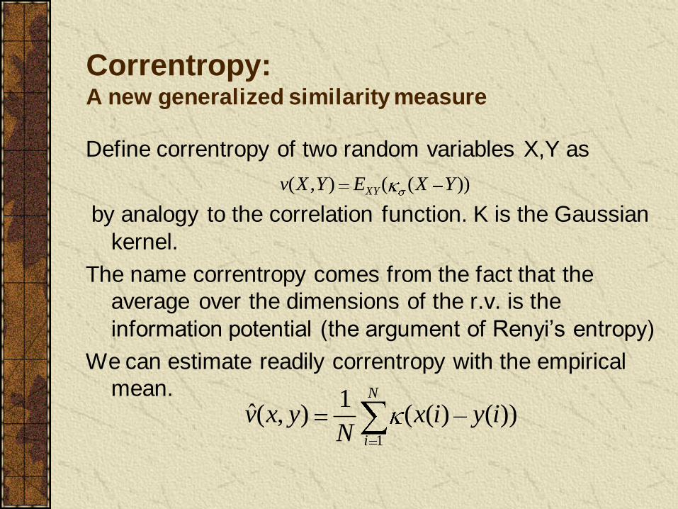
Correntropy:A new generalized similarity measure

Define correntropy of two random variables X,Y as

by analogy to the correlation function. K is the Gaussian

kernel.

The name correntropy comes from the fact that the

average over the dimensions of the r.v. is the

information potential (the argument of Renyi’s entropy)

We can estimate readily correntropy with the empirical

mean.

))((),( YXEYXv XY

N

i

iyixN

yxv1

))()((1

),(ˆ


Some Properties of Correntropy:

It has a maximum at the origin ( )

It is a symmetric positive function

Its mean value is the argument of the log of

quadratic Renyi’s entropy of X-Y (hence its name)

Correntropy is sensitive to second and higher order

moments of data (correlation only measures second

order statistics)

Correntropy estimates the probability of X = Y.

2/1

0

2

2 !2

)1(),(

n

n

nn

n

YXEn

yxv


Correntropy as a cost function versus MSE. 2

2

,

2

( , ) [( ) ]

( ) ( , )

( )

XY

x y

E

e

MSE X Y E X Y

x y f x y dxdy

e f e de

,

( , ) [ ( )]

( ) ( , )

( ) ( )

XY

x y

E

e

V X Y E k X Y

k x y f x y dxdy

k e f e de


Correntropy induces a metric in the sample space

(CIM) defined by

Correntropy uses different

L norms depending on the

actual sample distances.

This can be very useful for

outlier’s control and also to

improve generalization

2/1)),()0,0((),( yxvvYXCIM

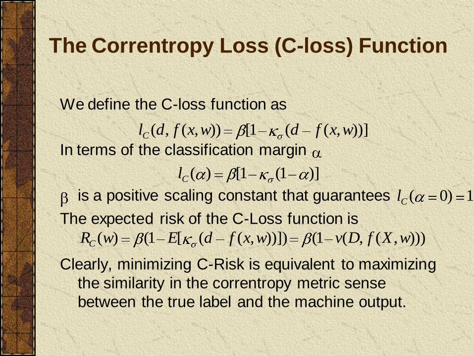
The Correntropy Loss (C-loss) Function

We define the C-loss function as

In terms of the classification margin

is a positive scaling constant that guarantees

The expected risk of the C-Loss function is

Clearly, minimizing C-Risk is equivalent to maximizing

the similarity in the correntropy metric sense

between the true label and the machine output.

))],((1[)),(,( wxfdwxfdlC

)]1(1[)(Cl

1)0(Cl

))),(,(1())]),(([1()( wXfDvwxfdEwRC

The Correntropy Loss (C-loss) Function

The C-Loss for several values of

The C-loss is non convex, but approximates better the

l0/1 loss and it is Fisher consistent.

The Correntropy Loss (C-loss) Function Training with the C-Loss

Can use backpropagation with a minor modification:

the injected error is now the partial of the C-Risk

w.r.t. the error

or

All the rest is the same!

n

nC

n

C

e

el

e

eR )()(

2

2

22

2

2exp

2exp1

)( nnn

nn

nC eee

ee

el

The Correntropy Loss (C-loss) Function Automatic selection of the kernel size

An unexpected advantage of the C-Loss is that it allows

for an automatic selection of the kernel size.

We select = 0.5 to give maximal importance to the

correctly classified samples

The Correntropy Loss (C-loss) Function How to train with the C-loss

The only disadvantage of the C-loss is that the

performance surface is non convex and full of local

minima.

I suggest to first train with MSE for 10-20 epochs, and

then switch to the C-loss

Alternatively can use the composite cost function

where N is the number of training iterations, and is set

by the user.

)()()1()( 2 wRN

wRN

wR C

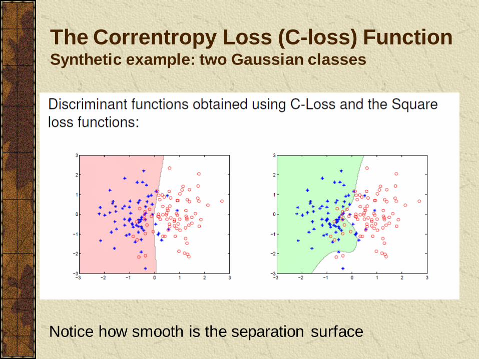
The Correntropy Loss (C-loss) Function Synthetic example: two Gaussian classes

Notice how smooth is the separation surface

The Correntropy Loss (C-loss) Function Synthetic example: more difficult case

Notice how smooth is the separation surface

The Correntropy Loss (C-loss) Function Wisconsin Breast Cancer Data Set

C-loss does NOT over train, so generalizes much better

than MSE

The Correntropy Loss (C-loss) Function Pima Indians Data Set

C-loss does NOT over train, so generalizes much better

than MSE

The Correntropy Loss (C-loss) Function But the point of switching affects performance

Conclusions

The C-loss has many advantages for classification:

• Leads to better generalization, as samples near the

boundary have less impact on training (the major cause

for overtraining with the MSE).

• Easy to implement - can be simply switched after

training with MSE.

• Computation complexity is the same as MSE and

backpropagation.

The open question is the search of the performance

surface. The switching between MSE and C-loss

afffects the final classification accuracy.

Statistical Learning Theory and the C-Loss cost function

Documents

Transcript of Statistical Learning Theory and the C-Loss cost function