Measurement Based Statistical Model for Path Loss ...
179
Measurement Based Statistical Model for Path Loss Prediction for Relaying Systems Operating in 1900 MHz Band by Masoud Dao Hamid A dissertation submitted to the College of Engineering at Florida Institute of Technology in partial fulfillment of the requirements for the degree of Doctor of Philosophy in Electrical Engineering Melbourne, Florida December 2014
Transcript of Measurement Based Statistical Model for Path Loss ...

Measurement Based Statistical Model for Path
Loss Prediction for Relaying Systems
Operating in 1900 MHz Band
by
Masoud Dao Hamid
A dissertation submitted to
the College of Engineering at
Florida Institute of Technology
in partial fulfillment of the requirements
for the degree of
Doctor of Philosophy
in
Electrical Engineering
Melbourne, Florida
December 2014

© Copyright 2014 Masoud Dao Hamid
All Rights Reserved
The author grants permission to make single copies ________________________


iii
Abstract
Measurement Based Statistical Model for Path Loss Prediction for
Relaying Systems Operating in 1900 MHz Band
by
Masoud Dao Hamid
Research Director: Ivica Kostanic, Ph.D.
Relays play important role in deployment of Long Term Evolution (LTE) and
LTE-Advanced systems. They are used to enhance coverage, throughput and
system capacity. The impact of the relay deployment on the network planning has
to be modeled so that the above mentioned goals can be achieved. For successful
modeling one needs to predict the path loss on the link between an eNodeB and a
relay station. The review of literature shows that there is a general shortage of
measured data to help empirical understanding of the propagation conditions in
relay environment. This dissertation aims at developing empirical path loss models
for relaying systems operating in 1900 MHz frequency band.
The path loss models are derived on a basis of an extensive measurement
campaign conducted in a typical suburban environment. The path loss modeling
takes into account the impact of the relay antenna height and therefore, an antenna
height correction factor is derived and included in the modeling. The parameters of

iv
those empirical models include the slope (m) and the intercept (PL0) for each level
of the examined relay heights. The parameters are determined from empirical
studies and through the appropriate linear regression process. In addition to path
loss modeling, the validity of some commonly used propagation models is
evaluated by comparing their predictions to the measurements.
It was found that the path loss may be modeled successfully with a slightly
modified log-distance propagation model. Two new different approaches for
development of the statistical propagation path loss models for relay systems has
been accomplished. The first approach includes fixed slopes and intercepts along
with a distance dependent antenna height correction. The second approach does not
include the relay antenna height correction factor but the height of the relay antenna
becomes part of the slope and intercept calculation. For both approaches, the results
show that model predictions are in good agreement with the measurement. As far
as the validity of the commonly used models is concerned, the comparison to the
measurements reveal that the applicability of those models for relaying
environment is still debatable. Some modifications are introduced in order to
improve the performance of these models. With the proposed correction factors all
the examined models perform adequately and with approximately the same
accuracy.

v
Table of Contents
Chapter 1: Introduction ……………………………………………………… 1
1.1 Motivation................................................................................................. 1
1.2 Objectives ................................................................................................. 3
1.3 Dissertation Outline................................................................................... 4
Chapter 2: Literature Review ………………………………………………... 6
2.1 Suggested Propagation Models for Relaying Scenarios .............................. 7
2.2 Impact of Receiver Antenna Height ........................................................... 7
Chapter 3: Relaying ………………………………………………………… 13
3.1 Motivation for Relaying .......................................................................... 13
3.2 Concept of Relaying ................................................................................ 16
3.3 Classifications of Relays ......................................................................... 17
Chapter 4: Background on Propagation Models …………………………. 19
4.1 Introduction ............................................................................................. 19
4.2 Basic Propagation Mechanisms ............................................................... 20
4.3 Propagation Models................................................................................. 22
4.3.1 Basic Propagation Models .............................................................. 23
4.3.1.1 Free Space Model ............................................................... 23
vi
4.3.1.2 Tow-Ray Model ................................................................. 26
4.3.2 Deterministic Models...................................................................... 27
4.3.3 Statistical Models ........................................................................... 28
4.3.3.1 Log Distance Path Loss Model ........................................... 29
4.3.3.2 Lee Model .......................................................................... 31
4.3.3.3 Hata Model ......................................................................... 33
4.3.3.4 COST-231 Model ............................................................... 34
4.3.3.5 IEEE 802.16j Channel Model ............................................. 35
4.3.3.6 WINNER II Model ............................................................. 39
4.3.3.7 3GPP models ...................................................................... 40
4.3.3.8 New relaying model ........................................................... 46
Chapter 5: Development of Propagation Model for Relay Stations ……... 48
5.1 Measurement Environment ...................................................................... 48
5.2 PCS Frequencies ..................................................................................... 49
5.3 Developing the Link between Relay Model and Existing Models ............ 50
5.4 Mathematical Modeling........................................................................... 51
Chapter 6: Measurement System and Procedure ………………………… 57
6.1 Equipment Description ............................................................................ 57
6.1.1 Transmitter ..................................................................................... 57
6.1.2 Transmit antenna ............................................................................ 58
6.1.3 Antenna Pattern .............................................................................. 59

vii
6.1.4 Receiver ......................................................................................... 63
6.1.5 Receive antenna .............................................................................. 65
6.1.6 Software ......................................................................................... 66
6.2 Receiver Noise Floor and Noise Figure ................................................... 68
6.3 Spectrum Clearing ................................................................................... 70
6.4 Procedure ................................................................................................ 72
Chapter 7: Path Loss Measurements for Relay Stations ………………… 80
7.1 Performance Analysis of Path Loss Measurements .................................. 80
7.2 Path Loss Models at Different Relay Antenna Heights ............................ 89
7.3 Received Signal Level models for Relay Stations .................................... 91
7.4 Path Loss Differences for the Examined Relay Heights ........................... 95
7.5 Relay Antenna Height Correction Factor ............................................... 100
7.5.1 For the case href=4 m:.................................................................... 111
7.5.2 For the case href=1.7 m: ................................................................. 120
Chapter 8: Developed Path Loss Models for Relaying Systems ………... 123
8.1 Performance Analysis of Existing Models ............................................. 123
8.1.1 Corresponding Assumptions for Considered Models ..................... 124
8.1.2 Simplified Versions of Existing Models ........................................ 126
8.1.3 Graphical and Statistical Evaluation.............................................. 130
8.1.4 Individual Evaluation of Existing Models ..................................... 135
8.2 Tuning of Existing Models .................................................................... 139
viii
8.2.1 Tuning of Standard Models........................................................... 140
8.2.2 Tuning of Existing Relaying Models............................................. 142
8.3 Performance Analysis of Tuned Models ................................................ 145
Chapter 9: Conclusions and Future Work ………………………………. 147
9.1 Summary and Conclusions .................................................................... 147
9.2 Future Work .......................................................................................... 149
Appendix: Antenna Pattern Data …………………………………………… 151
References …………………………………………………………………..… 157

ix
List of Figures
Figure 3.1: Resolving lack of coverage by using relays ........................................ 15
Figure 3.2: Three-node relay model...................................................................... 16
Figure 4.1: Propagation mechanisms .................................................................... 21
Figure 4.2: Two-Ray model ................................................................................. 26
Figure 4.3: Path loss vs. distance of 3GPP model for LOS and NLOS .................. 42
Figure 4.4: LOS probability as a function of distance for different environments.. 43
Figure 4.5: Path loss of 3GPP model considering LOS probability for urban
environment ......................................................................................................... 44
Figure 4.6: Path loss of 3GPP model considering LOS probability for suburban
environment ......................................................................................................... 45
Figure 4.7: Path loss of 3GPP model considering LOS probability for
suburban/rural environment ................................................................................. 45
Figure 6.1: Transmitter......................................................................................... 58
Figure 6.2: Transmit antenna ................................................................................ 58
Figure 6.3: Azimuth antenna pattern in polar coordinates ..................................... 60
Figure 6.4: Elevation antenna pattern in polar coordinates .................................... 61
Figure 6.5: Elevation antenna pattern in Cartesian coordinates ............................. 62
Figure 6.6: Receiver ............................................................................................. 64
Figure 6.7: Receive antenna ................................................................................. 66

x
Figure 6.8: Power measurements: numerical display ............................................ 67
Figure 6.9: Power measurements: graphical display ............................................. 68
Figure 6.10: Spectrum clearing measurement system ........................................... 70
Figure 6.11: Signal strength measurements at frequency 1925 MHz for 24 hours . 72
Figure 6.12: Illustration of the base station ........................................................... 74
Figure 6.13: Illustration of the mobile and relay stations ...................................... 75
Figure 6.14: Illustration of the receiver on a boom-lift.......................................... 76
Figure 6.15: Map of the area where the measurements were conducted. Transmitter
location is – Latitude: 28.064° N, Longitude: 80.624° W ..................................... 77
Figure 6.16: Measurement system ........................................................................ 78
Figure 7.1: Received signal level by latitude and longitude .................................. 82
Figure 7.2: Measured and predicted path loss for different relay heights ............... 83
Figure 7.3: Distribution of prediction error for h=1.7 m ....................................... 87
Figure 7.4: Distribution of prediction error for h=4 m .......................................... 87
Figure 7.5: Distribution of prediction error for h=8 m .......................................... 88
Figure 7.6: Distribution of prediction error for h=12 m ........................................ 88
Figure 7.7: Distribution of prediction error for h=16 m ........................................ 89
Figure 7.8: Measured and predicted received signal level for different relay heights
............................................................................................................................ 93
Figure 7.9: Distribution of path loss differences (PL(h=4) - PL(h=8)) .................. 96
Figure 7.10: Distribution of path loss differences (PL(h=4) - PL(h=12)) .............. 97

xi
Figure 7.11: Distribution of path loss differences (PL(h=8) - PL(h=12)) .............. 97
Figure 7.12: Distribution of path loss differences (PL(h=8) - PL(h=16)) .............. 98
Figure 7.13: Distribution of path loss differences (PL(h=12) - PL(h=16))............. 98
Figure 7.14: Distribution of path loss differences (PL(h=4) - PL(h=16)) .............. 99
Figure 7.15: Distribution of path loss differences (PL(h=1.7) - PL(h=4)).............. 99
Figure 7.16: Average relay antenna height correction factor (Δhm) for href=1.7 m 102
Figure 7.17: Average relay antenna height correction factor (ΔhR) for href=4 m .. 102
Figure 7.18: Path loss models based on the average relay antenna height correction
factor for href=1.7 m ........................................................................................... 104
Figure 7.19: Path loss models based on the average relay antenna height correction
factor for href=4 m .............................................................................................. 105
Figure 7.20: Prediction error based on the average relay antenna height correction
factor (Δhm) for href=1.7 m ................................................................................. 106
Figure 7.21: Prediction error based on the average relay antenna height correction
factor (ΔhR) for href=4 m ..................................................................................... 107
Figure 7.22: Illustration of Δℎ as a function of relay height and distance ............ 109
Figure 7.23: Relay antenna height correction factor (∆ℎ) as a funtion of distance
and relay height.................................................................................................. 113
Figure 7.24: Measurements compared to model predictions after implementation of
∆ℎ for href=4 m ................................................................................................... 115
Figure 7.25: Intercept (PL0) as a function of relay antenna height ....................... 118

xii
Figure 7.26: Slope (m) as a function of relay antenna height............................... 118
Figure 8.1: Comparison of model predictions with measurements for h=4 m ...... 131
Figure 8.2: Comparison of model predictions with measurements for h=8 m ...... 132
Figure 8.3: Comparison of model predictions with measurements for h=12 m .... 132
Figure 8.4: Comparison of model predictions with measurements for h=16 m .... 133

xiii
List of Tables
Table 1.1: Important LTE-Advanced parameters .................................................... 2
Table 4.1: Path loss exponent for different environments [35] .............................. 30
Table 4.2: Standard deviation for different environments ..................................... 31
Table 4.3: Intercept and slope values for different environments .......................... 32
Table 4.4: Path loss types for IEEE802.16j relay system ...................................... 36
Table 4.5: Parameters for the terrain type A/B/C .................................................. 38
Table 4.6: Standard deviation for different categories ........................................... 38
Table 4.7: Sub-scenarios of WINNER B5 model .................................................. 39
Table 4.8: LOS probability for different environments [8] .................................... 43
Table 4.9: Summary of path loss models and their restrictions ............................. 47
Table 5.1: The electromagnetic spectrum ............................................................. 49
Table 6.1: Transmit antenna technical specifications ............................................ 59
Table 6.2: Elevation angle and corresponding antenna gain .................................. 63
Table 6.3: Receiver inputs and their frequency ranges .......................................... 64
Table 6.4: Technical specifications of receive antennas ........................................ 65
Table 6.5: Parameters associated with the measurement campaign ....................... 77
Table 7.1: Relay path loss propagation model parameters..................................... 85
Table 7.2: Relay received signal level parameters ................................................ 92
Table 7.3: Average of path loss differences between relay heights........................ 96

xiv
Table 7.4: Slope and intercept differences for href =4 m ...................................... 110
Table 7.5: Slope and intercept differences for href =1.7 m ................................... 111
Table 7.6: Model comparison before and after implementation of ∆ℎ relative to the
measurements for href=4 m ................................................................................. 116
Table 7.7: Comparison between measurements and model predictions ............... 119
Table 7.8: Model comparison before and after implementation of ∆h relative to the
measurements for href=1.7 m .............................................................................. 122
Table 8.1: Models parameters assumptions for measurement campaign .............. 127
Table 8.2: Comparison between measurements and models' predictions ............. 134
Table 8.3: Comparison between measurements and tuned-models' predictions ... 146

xv
Acknowledgment
All thanks and praise is due to Allah the Almighty. I thank Him for His
countless bounties and generous blessings upon us. I thank Him for
providing me the opportunity and granting me the capability to successfully
complete this work.
I would like to express my deep and sincere gratitude to my advisor,
Dr. Ivica Kostanic. In addition to being an excellent advisor, I took most of
my classes with him. I admire his way of teaching and his deep knowledge in
his field. He simplifies complex concepts to their fundamental principles. The
knowledge I gained from classes he teaches and the experience I acquired
from working with him have made my academic and experimental
background better. Thank you for your continuous support, guidance,
attention and encouragement. I am privileged to have you as my advisor.
I am also very grateful to a number of people who supported me
throughout my research journey. First, I am thankful to my parents for their
endless love, support, prayers and patience during the time I studied abroad.
I would like to pass my special thanks to my wife for her love, support,
patience, and understanding during this long time of study. I also would like

xvi
to express my warmest thanks and gratitude to my kids for their support and
patience. My sincere gratitude goes to all my brothers, sisters, uncles and
friends for their support and encouragement. Finally, I extend my special
thanks and acknowledgement to my friend Sasie El-Hajajie for helping me in
the data collection process. I thank them all for what they have done to
achieve my goal and reach this very essential milestone in my academic life.

xvii
Dedication
To:
My father and mother for their love, prayers, endless support and
encouragement
My wife for her love, support, encouragement, patience and
understanding
My kids for their love
My brothers, sisters, uncles and friends for their love and support
In memory of my grandmother for being my first teacher

1
Chapter 1: Introduction
1.1 Motivation
The number of mobile cell phone users is increasing at the rapid pace. The
annual growth of data traffic is estimated to remain high. The global mobile data
traffic is expected to increase at the rate of 61 % from 2013 to 2018 [1]. The
number of mobile-connected devices is expected to exceed the world population by
the end of 2014 as reported in [1, 2]. This is due to user mobility and the ease of
installations of wireless communication systems. WiFi, WiMAX, 3G and 4G
cellular networks are some examples of cellular systems experiencing very high
growth. Current 3G systems are not capable of providing very high data rate to a
large number of users. Thus, there is a need for wireless access systems that can
accommodate such growth. Currently, the Third Generation Partnership Project
Long-Term Evolution (3GPP-LTE) and 3GPP-LTE-Advanced are being rolled out
by many operators to meet ever increasing demand for higher data rate and better
Quality of Service (QoS) [3].
LTE-Advanced is the upcoming global cellular technology that offers very
high throughput on air its interface. The envisioned data rates for 4G LTE wireless
systems can exceed 300 Mbps in the downlink (DL) and 75 Mbps in the uplink
(UL) within 20 MHz of paired spectrum. LTE-Advanced, on the other hand, is set

2
to provide data rate up to 1 Gbps and 500 Mbps in down link and uplink,
respectively [4]. Those high data rates are to be met by aggregating multi carriers
with scalable spectrum up to 100 MHz. In order to get this very high data rate,
high modulation schemes such as 16 QAM (Quadrature Amplitude Modulation)
and 64 QAM need to be used. Table 1.1 summarizes important requirements for
performance of the LTE-Advanced [5].
Table 1.1: Important LTE-Advanced parameters
Peak data rate (Gbps) DL 1 Antenna
configuration UL 0.5
Peak spectrum efficiency
(bps/Hz)
DL 30 (8x8)
UL 15 (4x4)
Average spectrum efficiency
(bps/Hz/cell)
DL
2.4
2.6
3.7
(2x2)
(4x2)
(4x4)
UL 1.2
2.0
(1x2)
(2x4)
Cell edge user throughput
(bps/Hz/cell/user)
DL
0.07
0.09
0.12
(2x2)
(4x2)
(4x4)
UL 0.04
0.07
(1x2)
(2x4)
Mobility up to 500 km/h
Bandwidth scalable bandwidth up to 100 MHz
Modulation scheme QPSK, 16 QAM and 64 QAM
One of most promising technology that helps LTE-Advanced meet these
requirements is the use of relays. Within LTE and LTE-Advanced, radio relays are

3
used to extend coverage, enhance capacity, increase throughput and provide overall
increase in the network performance [6-8]. In addition to performance
enhancements, relays are expected to be a viable cost efficient solution for
replacement of base stations [9,10]. When deployed, relays act like base stations
but without the need of wired connection to the backhaul. From the network
planning perspective one needs to be able to successfully model the impact of the
relay deployment within an LTE network. The first step in this modeling is the
prediction of the path loss on the link between the eNodeB and a relay station. The
review of literature shows that there is a general shortage of measured data
collection and understanding of the propagation conditions in relay environment.
The measurement campaign discussed in this dissertation is set up specifically to
evaluate the path loss encountered on eNodeB-relay link.
1.2 Objectives
The main objective of the research proposed in this dissertation is to develop
statistical path loss models for outdoor relaying systems in 1900 MHz frequency
band. The proposed models are derived to predict the radio signal path loss on the
link between eNodeB and relay stations (backhaul link). The path loss modeling
takes into account the impact of the relay antenna height and therefore, an antenna
height correction factor is included in the modeling. The models are based on field
measurements conducted in suburban environment. Two major contributions are
achieved. Firstly, propagation models are derived by conducting comprehensive

4
measurements and explaining the behavior of the path loss as a function of relay
station antenna height. Additionally, since many propagation models are already
coded and part of software packages that are used for deployments, it is of special
interest to establish a relationship between measurements and some of these
standard propagation models. Well known examples of the standard models are:
Hata-Okumura, Lee model, COST 231-Hata, COST 231 Walfisch-Ikegami, and
many other proprietary models. Application of standard propagation models for
modeling relay scenarios is examined and the appropriate correction factors are
derived.
1.3 Dissertation Outline
The dissertation is organized as follows. Chapter 2 provides a summary of
related work on path loss propagation models for relaying scenarios. Overview of
the concept of relaying and classification of relays are given in Chapter 3. General
background on propagation models and basic propagation mechanisms are
provided in Chapter 4. Chapter 5 presents the development of propagation models
for relay stations. In this chapter, developing the link between relay model and
other existing models is introduced. Empirical relay model derivation is then
provided. Chapter 6 is devoted to description of the procedure and equipment used
in the measurement campaign presented in this document. Chapter 7 proposes
propagation path loss models for eNodeB-relay link for multiple relay antenna
heights, provides statistical analysis for the proposed models and introduces a relay

5
antenna height correction factor. Chapter 8 presents the evaluation of the existing
models relative to the measurements, introduces some modifications of the original
forms of the existing models to make their prediction more reliable in relaying
environments. Finally, summary and some conclusions are drawn in Chapter 9.

6
Chapter 2: Literature Review
The concept of relaying (multi-hop) is not new. A classical three-node
relaying model was first introduced in early 1970's [11]. A simple relay channel
was proposed and an achievable lower bound to the capacity was established [12].
However there was no additional investigative study most likely because of non-
foreseeable applications at that time. Recently, the concept of relays has been
brought up again and proposed in the cellular network system such as WiMAX and
3GPP LTE-Advanced [13].
When deployed, relaying cellular networks consist of three links: BS-RS
(Base Station-Relay Station) link, BS-MS (Base Station-Mobile Station) link and
RS-MS (Relay Station-Mobile Station) link. These three links are also referred to
as backhaul link (the link between eNodeB and relay), direct link (the link between
eNodeB and end user) and access link (the link between relay and end user),
respectively. The work presented in this dissertation focuses on the path loss
evaluation encountered on eNodeB-relay link only. Backhaul link path loss and, in
particular, the impact of relay station antenna height on propagation link in
suburban areas need to be well understood so proper design can be offered for such
networks.

7
2.1 Suggested Propagation Models for Relaying
Scenarios
Whereas propagation models for BS-MS link have been widely studied in the
literature (Okumura, Hata, COST 231 and Lee models, just to name a few), far too
little attention has been paid to the BS-RS link. To this end, some of propagation
models have been suggested by 3GPP (3rd Generation Partnership Project) [8],
WINNER (Wireless World Initiative New Radio) [14] and IEEE 802.16j task
group [15]. Nonetheless, one general limitation of these models is that they are
developed from already existing propagation models that were derived under
completely different assumptions. Hence their applicability to relay scenarios need
to be examined. Another limitation is that the considered models were derived for
just certain levels of relay antenna height. Models in [8] and [14] were derived for
relay heights 5 m and 15 m, respectively, and therefore their validation for multiple
relay heights still needs to be performed.
2.2 Impact of Receiver Antenna Height
The impact of mobile station antenna height on the propagation channel of
BS-MS link has been extensively studied in [16-19]. In these studies, typical
mobile station antenna height was about 0.3-3 meters. Research on the effect of
relay station antenna height on BS-RS propagation link, on the other hand, has not
yet been adequate. To the best of author's knowledge, very view studies evaluate

8
the path loss on the eNodeB-relay link (BS-RS link) for different relay heights. In
this section, related work will be reviewed.
Quang Hien, et al. in [20] investigated the effect of receive antenna height
on the received signal level in a LTE-Advanced relaying scenario. The study
concentrated basically on the BS-RS link only. In this study, multi-frequency bands
were used and measurements were conducted in an urban environment. The
measurements were performed by locating the receiver in different positions in a
multi-floor building. The aim of using a multi-floor building is to represent
different levels of receiver antenna height. The obtained results show that higher
received signal levels are achieved for higher relay antenna heights. WINNER B5a
and B5f models for relaying scenarios were examined. Authors claimed that
whereas their results were in agreement with WINNER B5a model, disagreement
was pronounced comparing to WINNER B5f model. Study would have been more
interesting if the authors had proposed an empirical path loss model which can be
applied in similar scenarios.
Similar to the work done in [20], authors in [21] studied the impact of relay
antenna height on LTE-Advanced path loss channel model focusing on the BS-RS
link. Measurements of path loss values were performed at three levels of relay
antenna height. The experiments were carried out at frequency of 2.1 GHz in an
urban macro-cellular area. As expected, dependency of path loss on relay antenna

9
height was observed. The obtained path loss values decrease with the increase of
relay antenna height. Various existing propagation models, which could be applied
for BS-RS link, were then examined. Authors reported that the most striking result
to emerge from the data comparison was that the disagreement between the
obtained results and the IEEE 802.16j model was very obvious and on the order of
approximately 20 dB. Another pronounced mismatch was with WINNER B5f
model. These results were surprising because both IEEE 802.16j and WINNER B5f
models were proposed for relaying scenarios. A third interesting observation from
the study was that even though COST-231 Walfish-Ikegami model was not
designed for relaying deployment, it provided the closest results of path loss
prediction when compared to other models that were examined. Finally, a simple
statistical propagation model for relaying scenarios which takes into consideration
the influence of the relay antenna height was suggested. Nevertheless, studies in
[20, 21] conclude that the validity of the investigated models which were designed
for relaying systems is questionable.
Unlike [20] and [21], the study presented in [22] not only investigated the
impact of relay station antenna height on the received signal power of BS-RS link
but also analyzed the corresponding Signal to Interference Ratio (SIR). The study
included also the effect of the relay station antenna type i.e. (directional versus
omnidirectional configuration) on the BS-RS link performance. Results in this
study were based on data collected in a real urban macro-cell area operating in 3G

10
network deployment. Authors concluded that both relay station antenna height and
type affect the BS-RS link performance. Although increasing relay station antenna
height results in better received signal, using directional antenna to improve SIR
has a significant impact only in Line of Sight (LOS) conditions. Nevertheless, the
major concern of this study was the performance evaluation of the relay station
location rather than studying the propagation path loss models in the BS-RS link.
Authors in [23] provided new statistical propagation models for peer-to-peer
communication channel. Five links, namely, BS-MS, BS-RS, RS-RS, RS-MS and
MS-MS were considered. Models were developed based on measurements
performed in center of Bristol, UK. This study has shown that the path loss
decreases with higher antenna heights and with higher probability line of sight. The
study has gone some way towards enhancing the understanding of dependency of
shadowing and LOS probability on distance. However, the main focus of this study
was on peer-to-peer (MS-MS) links which have low antenna heights and short
distances.
Work in [24] presented measurements conducted in relay-deployed network
in an urban environment at frequency 3.5 GHz. BS-RS link path loss was analyzed
and compared to COST 231 and IEEE 802.16d models. Authors found out that
results of BS-RS link are in agreement with IEEE 802.16d. However, the

11
maximum height of relay station antenna was limited to 5 meters which is too low
for most relay scenarios.
In [25], comparison between different propagation models were made at two
levels of receiving antenna height. Unlike studies [20-24], where the measurements
were carried out in urban environment only, work presented in [25] investigated the
path loss in different environments. However, this study does not take in account
some propagation models proposed for relaying scenarios such as 3GPP and
WINNER.
Related work is to be found in [26]. Even though a statistical path loss model
was developed in this work, the receiver antenna height ranged only between 3 to 7
meters which is low according to proposed relay scenarios [8, 14].
Other work reported in [27, 28] considered a receiver antenna height up to 10
meters. Nevertheless, these studies neither suggest new propagation models nor
provide comparison with any of the existing models.
Reference [18] analyzed the influence of changing the antenna heights of
both transmitter and receiver on path loss models. However, this study concentrated
on indoor channel characterization.
In short, a number of important limitations, that previous work suffer from,
needs to be addressed. One major constrain is that the studied relay station antenna

12
heights considered to be low compared to proposed relay scenarios [8, 14]. Another
limitation is that, in most studies, no statistical path loss models were proposed and
if any, they were derived for urban environment and their validity for different
environments such as suburban or rural areas is questionable. Third, the validity of
the proposed models for relaying systems is still questionable and therefore, further
studies are required to examine their applicability across variety of scenarios.
Finally, in most of the related work, frequency bands that were used are different
from the one that will be used in this study. Hence, there is a need to cover these
gaps and this is the aim of the work described in this document.

13
Chapter 3: Relaying
3.1 Motivation for Relaying
As it was mentioned in chapter one, LTE-Advanced offers very high data rate
on the air interface due to the use of high modulation schemes such 16 QAM and
64 QAM. High modulation schemes require high Signal to Noise ratio (S/N). This
is because for a given power level, the bit energy decreases if the data rate
increases. It is also well known that for a given power the available data rate
decreases with the increasing of distance between base station and mobile device.
For instance, at cell edge the (S/N) is usually not high enough to use high
modulation schemes and consequently to have high data rate. One solution is to
increase the power of the base station so that the terminal at cell edge gets an
improved (S/N). Unfortunately, from practical prospective this solution is not
realistic. Increasing the power of one base station beyond certain level causes
interference with other signals from surrounding cells (inter cell interference). Even
if that would work for the down link (from base station to mobile station), it does
not work for the uplink (from mobile station to base station) because mobile device
has limited power. Therefore, to achieve high data rate, mobile station needs to be
close to the base station. Hence, the use of a traditional cellular radio network
would require a very high number of base stations to meet the required high data

14
rate. Unfortunately, adding more base stations results in potentially high
deployment costs and it does not appear economically reasonable. In [29], it is
shown that the deployment cost of a cellular radio network is directly proportional
to the number of base stations.
It is apparent that a novel solution is necessary for the very ambitious
throughput and coverage requirements of future systems. One of most promising
solutions is the deployment of relaying (multi-hop) technology. It promises to
reduce the deployment cost while enabling enhancement of coverage, throughput
and system capacity [6, 7, 10, 13, 30-33]. Relaying technique is considered a viable
solution for replacement of base stations. Relays cost significantly less than base
stations. The relays act like base stations but without the need of wired connection
to backhaul.
Relaying technique has been used typically for resolving the lack of signal
coverage in some areas. Shadowed and dead spot areas, tunnels, in building, stadia
and campus environments are some examples of low wireless signal areas. The
technique is implemented where the traffic is too low to justify the deployment of a
conventional base station. Relays can also be deployed to extend coverage where
the signal is not sufficient to access the base station like at cell edge. Relays can
provide temporary coverage in particular occasions such as sporting events, or in
emergency and disaster situations. Furthermore, mobile relays can provide access

15
to subscribers in high speed motion scenarios such as in airplanes or trains. Figure
3.1 shows an example of a relay deployment to enhance or provide coverage in
areas mentioned previously.
Figure 3.1: Resolving lack of coverage by using relays

16
3.2 Concept of Relaying
Figure 3.2 illustrates a simple three-node relay model. This model consists of
a base station, relay station and mobile station. As shown in the figure, the mobile
station can receive the signal from the base station through two different paths, the
one-hop direct link or the two-hop relaying link. In the one-hop direct link, the path
between the base station and the mobile station is called BS-MS link. In the two-
hop relaying link, a multi-hop relaying system consists of two links. The first link
is the link between the base station (eNodeB) and the relay station and it is referred
to as the BS-RS link or (backhaul link). The second link is the link between the
relay station and the mobile station (end user) and it is referred to as the RS-MS
link or (access link).
Figure 3.2: Three-node relay model

17
Since the relay station communicates both with the base station and the
mobile station, interference between the backhaul link and the access link may
occur. In order to avoid this interference, isolation between the two links is
required. Isolation can be achieved in several ways: frequency, time, and/or spatial
domains [34].
3.3 Classifications of Relays
There are different ways to classify relays. With respect to the relay's usage
of spectrum, relaying can be classified into outband and inband types. In outband
relaying type, backhaul link and access link operate in a different carrier frequency.
Therefore, interference between backhaul link and access link can be avoided by
obtaining the isolation between the two links in frequency domain. This approach is
referred to as Frequency Division Multiplexing (FDM). On contrary, in inband
relaying type, both backhaul link and access link operate in the same carrier
frequency. In this type of relaying, the isolation between the two links is obtained
in time domain. This approach is referred to as Time Division Multiplexing (TDM).
Another way to classify relays is according to how relay processes the
received signal. According to this approach, relays can be classified into amplify-
and-forward and decode-and-forward relays [6]. The former one is commonly
referred to as analog repeaters whereas the later one is referred to as digital
repeaters. The first type simply receives signals including noise and interference,

18
amplifies and then forwards them. This type of relays is very simple and has very
short processing time delay, but it also amplifies noise. Therefore, relays of this
type are mainly useful in high-SNR environments. Decode-and-forward relays, on
the other hand, decode and re-encode the received signal before forwarding it to
users. This means that this type of relays forwards the useful signal only but not
noise and interference. For that reason, decode-and-forward relays are useful in
low-SNR environments too. However, the processing time in this type is longer
which result into additional delay.
19
Chapter 4: Background on Propagation
Models
4.1 Introduction
In wireless communication system signals travel between transmit antenna
and receive antenna through a channel. The channel is a fundamental part of
wireless system deployment and has an essential role of the system performance. In
general, when the signal travels its level decreases with the increasing distance
between source (base station, relay station or mobile station) and destination
(mobile station, relay station or base station). The degradation in the transmitted
signal power as it propagates in space is referred to as path loss. Prediction of the
path loss is a fundamental task in cellular systems deployment. One of the
requirements of designing base stations in cellular networks is to have a basic
understanding of coverage areas of each base station. Finding the coverage area of
each base station through measurement is impractical since it can be very expensive
and time consuming process. Instead, engineers rely on propagation modeling that
estimates the average signal strength and consequently the path loss at any
particular distance from the base station. While overestimation of path loss can
result in extensive coverage overlaps, an underestimation can lead to coverage
holes. Path loss is a function of various factors such as free space losses,

20
diffraction, reflection, refraction, transmission frequency, terrain and many others.
Numerous propagation models have been derived and studied, however; there is no
single model can be applied for all the environments. As a result, the Quality of
Service (QoS) of the whole cellular network depends on the selection of most
suitable of the radio propagation model.
In this chapter some of the propagation mechanisms, namely, reflection,
diffraction and scattering, which occur as a result of obstacles' presence, are briefly
explained. Then, various propagation models which are used in assessing the
performance of a wireless system will be presented.
4.2 Basic Propagation Mechanisms
Unlike free space where the signal propagates without any obstacles, in
cellular mobile communication the signal is exposed to three basic effects:
Reflection: reflection occurs when a propagating wave impinges on an object which
is very large compared to its wavelength. Typical examples of such kind of objects
are surface of the earth, walls and buildings.
Diffraction: diffraction occurs when the path between the transmitter and the
receiver is obstructed by an object that has sharp irregular edges. As a result, waves
bend around and propagate behind the obstruction reaching the receiver even when

21
there is no LOS. This phenomenon is called shadowing because the receiver is
located in a shadowed region.
Scattering: scattering occurs when objects are on the order or less of the
wavelength of the radio signal. Typical examples of such kind of objects are street
signs, foliage and lamp posts. When a radio signal reaches such objects, it scatters
in many different directions. Figure 4.1 illustrates these three mechanisms.
Figure 4.1: Propagation mechanisms
As a mobile user moves throughout a coverage area, the instantaneous
received signal power is subject to the above mentioned three mechanisms.

22
Multiple copies of the signal (multipath propagation) would be presented at the
receiver and they may interfere constructively or destructively. Diffraction and
scattering result in a small scale fading. It describes the rapidly variation in the
instantaneous signal power when a mobile user moves over a short distance. On the
other hand, reflection causes a large scale fading. It characterizes the signal
variation over a larger distance. These variations are usually predicted by using
propagation models by averaging the received signal level at a particular distance
from the transmitter.
4.3 Propagation Models
One of the fundamental parameters of designing cellular communication
systems is the received signal level. In order to predict the average received signal
level, propagation models are used. In this regard, propagation modeling becomes a
very significant tool to study. Signal attenuation (or path loss) prediction and
received signal level prediction are two faces of the same coin. In other words, if
one is able to predict the median path loss then the median received signal level is
implicitly known. The path loss is simply the deference, expressed in decibels,
between the transmitted signal and the received signal power. Path loss includes all
possible losses which result from the free space propagation and other different
propagation mechanisms. In general, it is also function of other parameters like
antenna heights, carrier frequency, distance, environment type (urban, suburban or
rural) ... etc. Models that are used for predicting the path loss in macro-cells, which

23
are usually encountered in cellular networks, are called macroscopic propagation
models. There are many of them and they have different levels of accuracy and
complexity. In general, there is a tradeoff between model simplicity and its
accuracy. Macroscopic propagation models can be classified into three main
categories: basic propagation models, statistical propagation models and
deterministic models.
4.3.1 Basic Propagation Models
Basic propagation models are used to predict the path loss in a very simple
way. These basic models, by their very nature, give an approximated value of path
loss but they are introduced here to understand the other kinds of propagation
models which will be discussed later.
4.3.1.1 Free Space Model
The major assumption in free space propagation is that there is a clear line of
sight (LOS) between transmitter and receiver, meaning that no obstructions exist.
In other words, waves travel without reflection, diffraction, scattering, or any other
mechanisms. This model is used to predict the received signal power at a particular
distance. Satellite communication systems and microwave links are typical
example of such kind of models. The received signal power Pr at distance d from
the transmit antenna can be given as [35]:

24
𝑃𝑟 = 𝑃𝑇𝐺𝑇𝑋𝐺𝑅𝑋(4𝜋𝑑/𝜆)2
(4.1)
where
Pr - Received power at distance d from the transmitter
PT - Transmit power
GTX - Gain of transmitting antenna
GRX - Gain of receiving antenna
λ - Wave length
d - Distance between the transmitter and receiver
The propagation loss is usually expressed in decibels (dB) and it is given by
𝐿[dB] = 10log (𝑃𝑇𝑃𝑟) (4.2)
Therefore,
𝐿[dB] = 10log [(4𝜋𝑑/𝜆)2
𝐺𝑇𝑋𝐺𝑅𝑋] (4.3)
Since
𝜆 =𝑐
𝑓 (4.4)
where

25
c - Light velocity in space [3. 108 𝑚/𝑠𝑒𝑐]
f - Operating frequency
Substituting (4.4) in (4.3) one gets:
𝐿[dB] = 10log
[ (4𝜋𝑓𝑑𝑐 )
2
𝐺𝑇𝑋𝐺𝑅𝑋]
𝐿[dB] = −𝑔𝑇𝑋 − 𝑔𝑅𝑋 + 20log(𝑓) + 20log(𝑑) + 20log(4𝜋/𝑐)
(4.5)
Free space path loss, which represents the attenuation of the signal power, is
defined as the difference in dB between the effective transmitted power and
received power. When antenna gains are excluded, then the free space path loss
(PLFS) can be given as
𝑃𝐿𝐹𝑆[dB] = 32.44 + 20log(𝑓) + 20log(𝑑) (4.6)
where now the frequency f is in units of MHz and distance d in units of Km.
If d is expressed in miles then Eq. (4.6) can be written as:
𝑃𝐿𝐹𝑆[dB] = 36.5 + 20log(𝑓) + 20log(𝑑) (4.7)
Equations (4.6 ) and (4.7) are called Friis equations [36]. It is noteworthy to
observe that the free space path loss increases 20 decibel per decade of either

26
frequency or distance. In other words, free space path loss increases by 6 dB for
each doubling in either frequency or distance.
4.3.1.2 Tow-Ray Model
Unlike the free space propagation model where there is only a direct path
between the transmitter and the receiver, here, as the name says, the received signal
is sum of two components results from two different paths. First path is the direct
or LOS path and the second one is the ground reflected path. Figure 4.2 illustrates
this situation.
Figure 4.2: Two-Ray model
The formula of path loss for this model is expressed as [36]:

27
𝑃𝐿 = 40 log(𝑑) − 20 log(ℎ𝑏) − 20 log (ℎ𝑚) (4.8)
where,
d: Distance between transmitter and receiver in meters
hb: Height of the transmitter antenna in meters
hm: Height of the receiver (mobile) antenna in meters
It is remarkable that the path loss here increases by 40 dB/dec as a function of
distance or 12 dB by doubling the distance. It is also notable that the path loss
depends on antenna heights of transmitter and receiver. The other observation that
can be made here is that PL is frequency independent. One of the drawbacks of the
two ray model is that it underestimates the path loss because of two major reasons.
In practice, loss is almost always frequency dependent. Second, in this model the
ground was assumed flat and smooth which is in reality not the case. As was
mentioned earlier, the roughness of the terrain can lead to scattering which in turns
affects the total value of the signal power and consequently the path loss.
4.3.2 Deterministic Models
These types of models estimate the propagation path loss analytically. They
are based on physical laws of electromagnetic wave propagation. Deterministic
models consider all the propagation mechanisms and they tend to be accurate.
However, they are very complex because they require very large detailed data that

28
describe the propagation environment. Such data include all geometric information
about all the obstructions involved. The computational effort involved might be
massive or even beyond the capability of existing computers especially if the
environment is large and/or complex [37]. A typical example of deterministic
propagation models is a ray tracing model [38, 39].
4.3.3 Statistical Models
As it was mentioned in the previous section, deterministic models require
very large amount of information about the environment in which models are
applied. This is a very complex procedure. There is always a tradeoff between
simplicity and accuracy. The accuracy of path loss prediction might not be the
essential task of a wireless cellular system designer. The major concern here is the
overall area covered rather than specific signal power at a particular location. To
this end, statistical models are often more appropriate. Statistical propagation
models are usually based on field measurements, therefore, they are also called
empirical propagation models. In this type of models, extensive measurements of
path loss are made, and through statistical analysis of the data collected appropriate
equations are derived. Empirical models give satisfactory results when they are
used in similar environments to the one where the measurements were made. One
big advantage of such models is that they take into account all the propagation
parameters. However, in order for them to be applicable in environments other than

29
those used for their derivations, correction factors need to be added. In the
following some of the most popular empirical models are discussed.
4.3.3.1 Log Distance Path Loss Model
In general, the path loss at any particular location can be seen as consisting of
three major components: loss due to distance between transmitter and receiver, log
normal shadowing (large scale fading or slow fading) and small scale fading (fast
fading). In the first order approximation, the predicted path loss in [dB] at any
given distance d from the transmitter with respect to a reference distance d0 may be
described as log-distance path loss model and given by [35] :
𝑃𝐿(𝑑)[dB] = 𝑃𝐿0 +𝑚 log (𝑑
𝑑0) (4.9)
where
d0 - Reference distance (usually 1km or 1 mile in macro-cells and 100
m in microcells)
PL0 - Path loss at the reference distance (intercept)
d - Distance between transmitter and receiver
m - Slope in [dB/decade] which can be given as:
𝑚 = 10𝑛 (4.10)

30
where n is the path loss exponent. The values of PL0 and n depend on the
environment and they are usually determined through statistical analysis of path
loss data measurements. Table 4.1 gives typical values of n for different
propagation environment.
Table 4.1: Path loss exponent for different environments [35]
Environment Path loss exponent (n)
Free space 2
Urban area cellular radio 2.7-3.5
Shadowed urban cellular radio 3-5
In building line of sight 1.6-1.8
Obstructed in building 4-6
Obstructed in factories 2-3
Equation (4.9) expressed the average large scale path loss at a given distance
(d). Graphically, PL is a linear function of (d) in logarithmic domain.
Log Normal Shadowing
When the actual path loss data are plotted, they show variations about the
median path loss given by the model in (4.9). The variations are introduced by log
normal shadowing which occurs due the fact that different locations at the same
distance from the transmitter might have different environment and therefore the
path loss value is different. The PL(d) can be considered as a random variable that
is normally distributed in log-domain [35] and it is given as:

31
𝑃𝐿(𝑑)[dB] = 𝑃𝐿0 +𝑚 log (𝑑
𝑑0) + 𝑋𝜎 (4.11)
where 𝑋𝜎 is a log normally distributed random variable that describes the
shadowing effects and it can be expressed as:
𝑋𝜎 ∼ 𝒩(0, 𝜎)
The operator expressed by (~) means that 𝑋𝜎 is a zero mean Gaussian
distributed random variable with a standard deviation of 𝜎. As the model becomes
more accurate, the standard deviation 𝜎 of the unexplained portion (𝑋𝜎) of path loss
becomes smaller. Similar to the path loss exponent n, 𝜎 is environmentally
dependent. Table 4.2 shows some typical values of 𝑋𝜎 for different environments.
Table 4.2: Standard deviation for different environments
Environment Standard deviation (𝝈) in dB
Rural 5-7
Suburban 6-8
Urban 8-10
Dense urban 8-12
4.3.3.2 Lee Model
Lee model is one of the most popular and widely used path loss models. It is
known for its simplicity along with its reasonable prediction accuracy [40]. Lee
model was initially derived for frequencies around 900 MHz. Later on, the model

32
was extended to frequencies up to 2 GHz [40]. The path loss form of the model is
provided relative to reference conditions and is given as [41]:
𝑃𝐿𝐿𝑒𝑒 = 𝑃𝐿0 +𝑚log(𝑑
𝑑0) − 15log(
ℎ𝑡ℎ𝑡𝑟𝑒𝑓
) − 10log(ℎ𝑟ℎ𝑟𝑟𝑒𝑓
) (4.12)
where:
PL0 - Path loss at reference distance (d0) in [dB]
m - Slope in [dB/decade]
d - Transmitter-receiver separation in [km]
d0 - Reference distance (1.609 km)
ht - Transmitter antenna height in [m]
htref - Reference transmitter antenna height (30.48 m)
hr - Receiver antenna height in [m]
hrref - Reference receiver antenna height (3.048 m)
The intercept (PL0) and the slope (m) for different environments at 900 MHz
are provided in Table 4.3.
Table 4.3: Intercept and slope values for different environments
PL0 @ f0=900 MHz PL0 [dB] m [dB/decade]
Open area 95 43.5
Suburban 107.7 38.4
Urban (Philadelphia) 116 36.8
Urban (Newark) 110 43.1
33
Whereas the slope (m) remains the same for frequencies different than f0,
frequency correction factor for the intercept (PL0) is given by:
𝑃𝐿0(𝑓) = 𝑃𝐿0(𝑓0) + 20log(𝑓
𝑓0) (4.13)
4.3.3.3 Hata Model
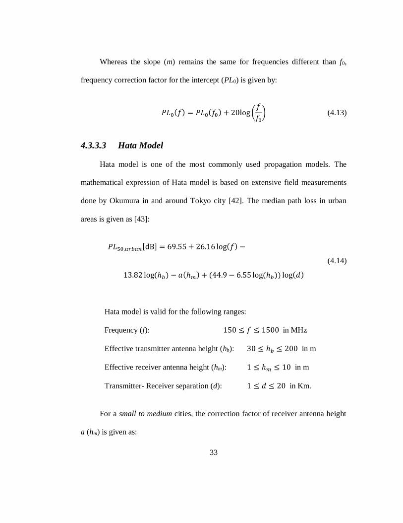
Hata model is one of the most commonly used propagation models. The
mathematical expression of Hata model is based on extensive field measurements
done by Okumura in and around Tokyo city [42]. The median path loss in urban
areas is given as [43]:
𝑃𝐿50,𝑢𝑟𝑏𝑎𝑛[dB] = 69.55 + 26.16 log(𝑓) −
13.82 log(ℎ𝑏) − 𝑎(ℎ𝑚) + (44.9 − 6.55 log(ℎ𝑏)) log(𝑑)
(4.14)
Hata model is valid for the following ranges:
Frequency (f): 150 ≤ 𝑓 ≤ 1500 in MHz
Effective transmitter antenna height (hb): 30 ≤ ℎ𝑏 ≤ 200 in m
Effective receiver antenna height (hm): 1 ≤ ℎ𝑚 ≤ 10 in m
Transmitter- Receiver separation (d): 1 ≤ 𝑑 ≤ 20 in Km.
For a small to medium cities, the correction factor of receiver antenna height
a (hm) is given as:

34
𝑎(ℎ𝑚)[dB] = (1.1 log(𝑓) − 0.7)ℎ𝑚 − (1.56 log(𝑓) − 0.8) (4.15)
For large cities, it is given as:
𝑎(ℎ𝑚)[dB] = {8.29(log(1.54ℎ𝑚))
2 − 1.1 for 150≤f ≤200
3.2(log(11.75ℎ𝑚))2 − 4.97 for 200<f≤1500
(4.16)
Default environment for Hata model is urban environment. If the predictions
of path loss are done in different environment, corrections need to be applied.
For suburban areas the model is given as:
𝑃𝐿50[dB] = 𝑃𝐿50,𝑢𝑟𝑏𝑎𝑛 − 2(log(𝑓
28))
2
− 5.4 (4.17)
For open rural areas the model is given as:
𝑃𝐿50[dB] = 𝑃𝐿50,𝑢𝑟𝑏𝑎𝑛 − 4.78(log(𝑓))2 + 18.33 log(𝑓) − 40.94 (4.18)
4.3.3.4 COST-231 Model
It also known as COST-Hata model. The European Co-operative for
Scientific and Technical research (EURO-COST) established the COST-231
working committee to introduce COST-231 model which is considered as an
extended version of Hata model to be applicable up to 2 GHz. The frequency range
for this model is 1500 MHz- 2000 MHz. The model is widely used for predicting
the median path loss in mobile wireless systems and its formula is given by [44]:

35
𝑃𝐿[dB] = 𝐴 + 𝐵log(𝑑) + 𝐶𝑚 − 𝑎(ℎ𝑚) (4.19)
𝐴 = 46.3 + 33.9 log(𝑓) − 13.82 log (ℎ𝑏) (4.20)
𝐵 = 44.9 − 6.55 log (ℎ𝑏) (4.21)
where the parameters f, hb, hm, and d are the same as defined in Hata model,
a (hm) is defined in equation (4.15), and
𝐶𝑚[𝑑𝐵] = {
0, for medium sized city and suburban areas
3, for metropolitan centers
The COST231 model is restricted to the following range of parameters:
Frequency (f): 1500 ≤ 𝑓 ≤ 2000 in MHz
Effective transmitter antenna height (hb): 30 ≤ ℎ𝑏 ≤ 200 in m
Effective receiver antenna height (hm): 1 ≤ ℎ𝑚 ≤ 10 in m
Transmitter- Receiver separation (d): 1 ≤ 𝑑 ≤ 20 in Km.
4.3.3.5 IEEE 802.16j Channel Model
This model was developed by IEEE relay task group. It is based on SUI
(Stanford University Interim) model and was extended in 2007 to cover relay
scenarios in IEEE 802.16j WiMAX systems [45]. The SUI model [46] is based on
extensive field measurements collected at 1.9 GHz across the United States in 95
macro cells. The model was mainly derived for suburban areas with three most
common terrain types, namely A, B and C. Type A describes areas which are hilly

36
with moderate-to-heavy tree densities, and it is associated the maximum path loss.
Type C applies to areas which are mostly flat with light tree densities and which
have the minimum path loss. Type B has a moderate path loss and it represents
either hilly terrains with light tree densities or mostly flat terrains with modest to
heavy tree densities. In 2007, IEEE802.16 Relay Task Group developed the SUI
model and introduced the IEEE802.16j model to cover nine categories of path loss
for relay systems [15]. The path loss types are given in Table 4.4.
Table 4.4: Path loss types for IEEE802.16j relay system
Category Description LOS/NLOS
Type A
Macro-cell suburban, ART to BRT
for hilly terrain with moderate-to-heavy tree densities.
LOS/NLOS
Type B Macro-cell suburban, ART to BRT
for intermediate path-loss condition LOS/NLOS
Type C Macro-cell suburban, ART to BRT
for flat terrain with light tree
densities
LOS/NLOS
Type D Macro-cell suburban, ART to ART LOS
Type E Macro-cell, urban, ART to BRT NLOS
Type F Urban or suburban, BRT to BRT LOS/NLOS
Type G Indoor Office LOS/NLOS
Type H Macro-cell, urban, ART to ART LOS
Type J Outdoor to indoor NLOS
Note: ART (Above Roof Top), BRT (Below Roof Top)

37
The IEEE802.16j path loss model for types A/B/C is given in [15] and can be
expressed as:
𝑃𝐿[dB] =
{
20 log(4𝜋𝑑
𝜆) + 𝑠 for 𝑑 ≤ 𝑑0
′
𝐴 + 10𝛾 log(𝑑
𝑑0) + ∆𝑃𝐿𝑓 + ∆𝑃𝐿ℎ + 𝑠 for 𝑑 > 𝑑0
′ (4.22)
where
𝐴 = 20 log(4𝜋𝑑0
′
𝜆) (4.23)
𝑑0′ = 𝑑010
−(∆𝑃𝐿𝑓+∆𝑃𝐿ℎ
10𝛾) (4.24)
𝛾 = 𝑎 − 𝑏ℎ𝑏 +𝑐
ℎ𝑏 (4.25)
∆𝑃𝐿𝑓[dB] = 6 log (𝑓
2000) (4.26)
∆𝑃𝐿ℎ[dB] = {−10 log(
ℎ𝑟3) for ℎ𝑟 ≤ 3
−20 log(ℎ𝑟3) for 3 < ℎ𝑟 < 10
(4.27)
where
d0 =100 [m]
λ - Wavelength [m]
γ - Path loss exponent
f - Operating frequency [MHz]
hr - Receiver antenna height [m]
hb - Base station antenna height [m]

38
d - Transmitter- Receiver separation [m]
ΔPLf - Correction factor for the frequency [dB]
ΔPLh - Correction factor for the receiver antenna height [dB]
a, b and c are constants and they depend on the terrain type as provided in
Table 4.5.
Table 4.5: Parameters for the terrain type A/B/C
Model parameter Terrain A Terrain B Terrain C
a 4.6 4 3.6
b [m-1] 0.0075 0.0065 0.005
c [m] 12.6 17.1 20
The parameter (s) in equation (4.22) represents the shadowing effect and it
has lognormal distribution. The typical value of the standard deviation of (s) for the
various categories is listed in Table 4.6.
Table 4.6: Standard deviation for different categories
Category Type
A
Type
B
Type
C
Type
D
Type
E
Type F Type G
LOS NLOS LOS NLOS
s [dB] 10.6 9.6 8.2 3.4 8.0 2.3 3.1 3.1 3.5
Restrictions to IEEE802.16j model are:
hb is 10-80 [m]

39
hr is 2-10 [m]
d is 0.1-8 [km]
4.3.3.6 WINNER II Model
This model was developed by IST-WINNER II project [14]. It covers a wide
range of propagation scenarios and environments. Path loss model for the different
WINNER scenarios have been developed based on measurements conducted within
WINNER, as well as results from the open literature. Among these scenarios are
the path loss models for fixed relays (i.e., stationary feeders), namely the scenario
B5 which it further divided into five sub-scenarios according to the relay location
as it illustrated in Table 4.7.
Table 4.7: Sub-scenarios of WINNER B5 model
Sub-scenario LOS/NLOS Transmitter
location
Receiver
location
B5a LOS Above rooftop Above rooftop
B5b LOS Street level Street level
B5c LOS Below rooftop Street level
B5d NLOS Above rooftop Street level
B5f LOS/NLOS Above rooftop Below/above rooftop
Based on [14], WINNER B5f sub-scenario is the most appropriate channel
model to predict the path loss for the link between the base station (i.e. eNodeB)
and relay station (backhaul link). WINNER B5f model takes into account both LOS

40
and NLOS conditions where the base station antenna height is above the rooftop
level and the relay station antenna height is either above or below the rooftop level.
According to [14], the path loss model for various WINNER scenarios are
typically given as:
𝑃𝐿[dB] = 𝐴 log(𝑑) + 𝐵 + 𝐶 log (𝑓
5) (4.28)
Where A=23.5, B=57.5 and C=23 for the sub-scenario B5f which is suitable
for predicting the path loss in urban areas, and
f - Frequency of operation [GHz], 2 GHz < f < 6 GHz
d - Base station- Relay station separation [m], 30 m < d < 1.5 km
It is important to note that this model was derived for base station antenna
height (hBS=25 m) and relay station antenna height (hRS=15 m).
4.3.3.7 3GPP models
3rd Generation Partnership Project suggested some propagation models for
predicting path loss in various environments [8, 47]. Among them were models
dedicated to BS-RS links. Those models distinguish between two scenarios, namely
LOS and NLOS. The models expressions are given by:
𝑃𝐿𝐿𝑂𝑆[dB] = 100.7 + 23.5 log(𝑑) (4.29)

41
and
𝑃𝐿𝑁𝐿𝑂𝑆[dB] = 125.2 + 36.3 log(𝑑) (4.30)
Where d in [km] is the distance between the base station and the relay station.
While equation (4.29) is used when the direct component LOS is dominant which
occurs when there are no obstacles between the transmitter and the receiver,
equation (4.30) is used otherwise (NLOS scenario). Path loss models in equations
(4.29) and (4.30) were derived under the following conditions:
f - Operating frequency [2 GHz]
hbs - Base station antenna height [30 m]
hrs - Relay station antenna height [5 m]
And the log-normal shadowing standard deviation was assumed to be 6 dB.
The path loss expressed in (4.29) and (4.30) are plotted in Figure 4.3. The
figure shows significant difference in path loss value between LOS and NLOS
conditions. For example, at 200 m distance, the path loss in the case of LOS is
about 85 dB whereas the path loss in the case of NLOS is 100 dB, i.e. the path loss
in LOS condition is smaller by 15 dB. This difference increases with increasing
distance between base station and relay station. The main difference between the
two path loss curves in Figure 4.3 is in the vertical interceptions and the slope.

42
Figure 4.3: Path loss vs. distance of 3GPP model for LOS and NLOS
In general, when relay station is close to base station, there is a high
probability that LOS is dominant. On the contrary, for far distances, NLOS
condition is more likely. The LOS probability is a function of different
environmental factors, including clutter, street canyons, and distance. The LOS
probability for different environments is given in Table 4.8.
The dependency of LOS on the distance for various environments is shown in
Figure 4.4.
102
103
50
60
70
80
90
100
110
120
130
140
150
Distance [m]
Path
Loss [
dB
]
NLOS
LOS

43
Table 4.8: LOS probability for different environments [8]
Environment LOS probability function
Urban 𝑝(𝑑) = min(
0.018
𝑑, 1) (1 − 𝑒−(
𝑑0.072
)) + 𝑒−(𝑑
0.072)
Suburban 𝑝(𝑑) = 𝑒−(𝑑−0.01)/0.23
Suburban/Rural 𝑝(𝑑) = 𝑒−(𝑑−0.01)/1.15
Figure 4.4: LOS probability as a function of distance for different environments
As Table 4.8 and Figure 4.4 show, LOS condition is more dominant in rural
and suburban areas than urban ones. For example, at 200 m distance, the LOS
probability is about 15%, 44%, and 85% for urban, suburban and rural
environment, respectively.
101
102
103
0
0.1
0.2
0.3
0.4
0.5
0.6
0.7
0.8
0.9
1
Distance [m]
LO
S P
robabili
ty
Urban
Suburban
Suburban/Rural

44
Taking LOS probability into consideration, the combined path loss is given
as:
𝑃𝐿(𝑑) = 𝑝(𝑑). 𝑃𝐿𝐿𝑂𝑆 + [1 − 𝑝(𝑑)].𝑃𝐿𝑁𝐿𝑂𝑆 (4.31)
Figure 4.5, 4.6 and 4.7 describe the behavior of path loss as a function of
distance in LOS, NLOS and combined LOS/NLOS conditions for urban, suburban
and rural environments, respectively.
Figure 4.5: Path loss of 3GPP model considering LOS probability for urban
environment
102
103
50
60
70
80
90
100
110
120
130
140
150
Distance [m]
Path
Loss [
dB
]
NLOS
LOS
LOS/NLOS

45
Figure 4.6: Path loss of 3GPP model considering LOS probability for suburban
environment
Figure 4.7: Path loss of 3GPP model considering LOS probability for
suburban/rural environment
102
103
50
60
70
80
90
100
110
120
130
140
150
Distance [m]
Path
Loss [
dB
]
NLOS
LOS
LOS/NLOS
102
103
50
60
70
80
90
100
110
120
130
140
150
Distance [m]
Path
Loss [
dB
]
NLOS
LOS
LOS/NLOS

46
For urban areas, as presented in Figure 4.5, the path loss follows the LOS
curve when relay station is close to base station (for d smaller than 40 m). On the
other hand, as relay station further away from base station (for d greater than 400
m), the path loss follows the NLOS curve. Roughly in the range between 30 m and
300 m, the path loss is considered as a combination between LOS and NLOS
conditions. In the cases of suburban areas (Figure 4.6) and suburban/rural areas
(Figure 4.7), the combined path loss is pronounced roughly in the range between 50
m and 700 m, and between 100 m and 4 km, respectively. Note that the combined
path loss is only in average sense. However, in practical scenarios, relay station can
either be in LOS or NLOS with base station, not both.
4.3.3.8 New relaying model
This model was developed based on measurements carried out in a typical
urban medium city of Belfort, France [21]. The model was proposed to predict path
loss encountered on the link between the base station and relay station. The model
was specifically derived for LTE-Advanced relaying systems operating in urban
environments. The proposed model takes into account the impact of relay antenna
height and it is given by:
𝑃𝐿[dB] = 34 log(𝑑) + 5 + 26log (20 − ℎ𝑅𝑆) (4.32)
where d in [m] is distance between base station and relay station, hRS in [m] is
the relay station antenna height. The model is valid for predicting path loss in the

47
relay link operates in 2.1 GHz band in NLOS conditions and with d ranges from
20-1000 m. The relay height is limited up to 15 m and the error standard deviations
are in the range of 7-8 dB [21].
Each individual propagation model has its own set of assumptions and is
restricted to a specific range of parameters under which it was derived. When a
propagation model is used to predict path loss outside of the specified parameter
range, its validity becomes questionable. Table 4.9 summarizes the range of
parameters under which the previously mentioned propagation models were
derived.
Table 4.9: Summary of path loss models and their restrictions
Model
Receiver
antenna
height (hr) in
[m]
Transmitter
antenna
height (hb) in
[m]
Distance
(d) in [km]
Operating
frequency (f)
in [MHz]
Hata 1-10 30-200 1-20 150-1500
COST-231 1-10 30-200 1-20 1500-2000
IEEE 802.16j 1-10 10-80 0.1-8 1900-11000
WINNER II 15 25 0.03-1.5 2000-6000
3GPP 5 30 NS 2000
Lee 1-15 20-100 up to 20 850-2000
Relay model [21]
4-15 22 0.02-1 2100
48
Chapter 5: Development of Propagation
Model for Relay Stations
5.1 Measurement Environment
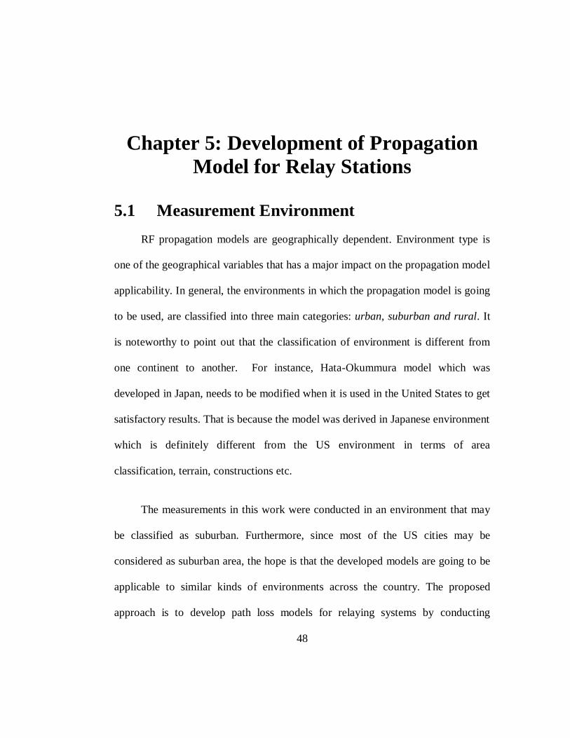
RF propagation models are geographically dependent. Environment type is
one of the geographical variables that has a major impact on the propagation model
applicability. In general, the environments in which the propagation model is going
to be used, are classified into three main categories: urban, suburban and rural. It
is noteworthy to point out that the classification of environment is different from
one continent to another. For instance, Hata-Okummura model which was
developed in Japan, needs to be modified when it is used in the United States to get
satisfactory results. That is because the model was derived in Japanese environment
which is definitely different from the US environment in terms of area
classification, terrain, constructions etc.
The measurements in this work were conducted in an environment that may
be classified as suburban. Furthermore, since most of the US cities may be
considered as suburban area, the hope is that the developed models are going to be
applicable to similar kinds of environments across the country. The proposed
approach is to develop path loss models for relaying systems by conducting

49
comprehensive measurements and explaining the behavior of the path loss as a
function of distance and relay station antenna height. Since the model is based on
field measurements, it is statistical in nature and it falls into the category of other
statistical macroscopic propagation models that have been covered in chapter 4.
5.2 PCS Frequencies
The electromagnetic spectrum covers a wide range of frequencies. However,
practical bands used in radio communication range from 3 kHz to 300 GHz as it is
shown in Table 5.1. The corresponding wavelengths in free space vary from 100
km to 1 mm.
Table 5.1: The electromagnetic spectrum
Category Acronym Frequency Wavelength (λ)
Extremely Low Frequency ELF < 3 kHz > 100 km
Very Low Frequency VLF 3 kHz-30 kHz 10 km-100 km
Low Frequency LF 30 kHz-300 kHz 1 km-10 km
Medium Frequency MF 300kHz-3 MHz 100 m-1 km
High Frequency HF 3 MHz-30 MHz 10 m-100 m
Very High Frequency VHF 30 MHz-300 MHz 1 m-10 m
Ultra High Frequency UHF 300 MHz-3 GHz 10 cm-1 m
Super High Frequency SHF 3 GHz-30 GHz 1 cm-10 cm
Extra High Frequency XHF 30 GHz-300 GHz 1 mm-1 cm

50
Most mobile radio communication applications are located in the frequency
bands from 30 MHz to 3 GHz (VHF/UHF bands). In these bands the corresponding
wavelength runs from 10 cm to 10 m. Therefore, VHF/UHF are the most suitable
bands for wireless communications due to the fact that the antenna size needs to be
comparable to the wavelength. More specifically, Personal Communication Service
(PCS), which describes any of many types of wireless voice and/or data
communication systems, are provided in the 1850-1990 MHz band. This band is
commonly referred to as 1900 MHz band.
The measurements in this work were taken place in 1900 MHz band and
therefore the model is going to be strictly applicable for that frequency.
Nevertheless, other models were developed for one frequency and then they have
been shown that with some minor modifications can be extended to other frequency
ranges.
5.3 Developing the Link between Relay Model
and Existing Models
There are many propagation models that are already coded, and they are part
of software packages that are used for development. Well-known examples of these
models are Hata model, COST 231-Hata model, Lee model etc. To this end, an
introduction of a new model is much easier if it relies on the ones that already exist.
One of the goals of this research is to examine the difference between

51
measurements and one or more of the standard models and then derive correction
factors so these models can be used in relaying scenarios. In other words, a link to
the already coded standard models can be established by some modifications on
existing software. Consequently, software implementation of the developed models
will be straightforward without need to implement new codes to introduce new
models.
5.4 Mathematical Modeling
The approach here is to develop an empirical propagation path loss model
that explains the observed data. In the first order approximation, the predicted path
loss in [dB] at any given distance (d) with respect to a reference distance (d0) may
be described using the log-distance path loss model as it was given by equation
(4.9) in Chapter 4. Recalling the equation:
𝑃𝐿(𝑑) = 𝑃𝐿0 +𝑚 log (𝑑
𝑑0) (5.1)
The parameters of the model, (m) the slope and 𝑃𝐿(𝑑0) the median path loss
at the (d0), are determined through statistical analysis of measurements collected
across various system configurations. The optimization of the path loss model
given in (5.1) can be achieved by first comparing measured and predicted values of
path loss, and then using the MMSE (Minimum Mean Square Error) method to

52
minimize the difference between predictions and measurements. Considering a
measurement process, then for every measurement point one can write:
𝑃𝐿𝑝𝑖 = 𝑃𝐿0 +𝑚 log (𝑑𝑖𝑑0) (5.2)
and
𝑃𝐿𝑚𝑖 = 𝐸𝑅𝑃 − 𝑃𝑟𝑖 (5.3)
where
PLpi: Predicted path loss for the ith point
PLmi: Measured path loss for the ith point
ERP: Effective Radiated Power
Pri: Received power at point i
The difference between measured and predicted path loss value for the ith
point is expressed as:
𝛿𝑖 = 𝑃𝐿𝑚𝑖 − 𝑃𝐿𝑝𝑖 (5.4)
where δi is the prediction error for the ith point and i=1, 2, ... N.
Substituting (5.2) into (5.4), one may write:

53
𝛿𝑖 = 𝑃𝐿𝑚𝑖 − 𝑃𝐿0 −𝑚 log(𝑑𝑖𝑑0) (5.5)
Taking all measurement points (N) into account, the expression in (5.5) may
be written in a matrix format as:
[ 𝛿1
𝛿2
⋮
𝛿𝑁]
=
[ 𝑃𝐿𝑚1
𝑃𝐿𝑚2
⋮
𝑃𝐿𝑚𝑁]
− 𝑃𝐿0
[ 1
1
⋮
1 ]
− 𝑚
[ log (
𝑑1𝑑0)
log (𝑑2𝑑0)
⋮
log (𝑑𝑁𝑑0)]
(5.6)
The objective here is to determine the optimum values of PL0 and m that
minimize the norm of the prediction error vector δ. In other words, the cost
function given by:
𝐽(𝜹) = 𝜹𝑇𝜹 =∑𝛿𝑖2
𝑁
𝑖=1
(5.7)
needs to be minimized.
By substituting (5.6) into (5.7), one may write:

54
𝐽(𝜹) =∑
(
[ 𝑃𝐿𝑚1
𝑃𝐿𝑚2
⋮
𝑃𝐿𝑚𝑁]
− 𝑃𝐿0
[ 1
1
⋮
1 ]
− 𝑚
[ log (
𝑑1𝑑0)
log (𝑑2𝑑0)
⋮
log (𝑑𝑁𝑑0)]
)
2
𝑁
𝑖=1
(5.8)
To get the minimal sum of the error squared, the partial derivative of
equation (5.8) with respect to PL0 and m needs to be zero.
First, considering the partial derivative of (5.8) with respect to PL0, one gets:
𝜕𝐽(𝜹)
𝜕𝑃𝐿0= 2∑
(
[ 𝑃𝐿𝑚1
𝑃𝐿𝑚2
⋮
𝑃𝐿𝑚𝑁]
− 𝑃𝐿0
[ 1
1
⋮
1 ]
− 𝑚
[ log (
𝑑1𝑑0)
log (𝑑2𝑑0)
⋮
log (𝑑𝑁𝑑0)]
)
= 0
𝑁
𝑖=1
(5.9)
Simplifying and rearranging (5.9), one may write:
∑𝑃𝐿𝑚𝑖
𝑁
𝑖=1
− 𝑁 ∗ 𝑃𝐿0 = 𝑚∑log(𝑑𝑖𝑑0)
𝑁
𝑖=1
(5.10)
Now, considering the partial derivative of (5.8) with respect to m, one gets:
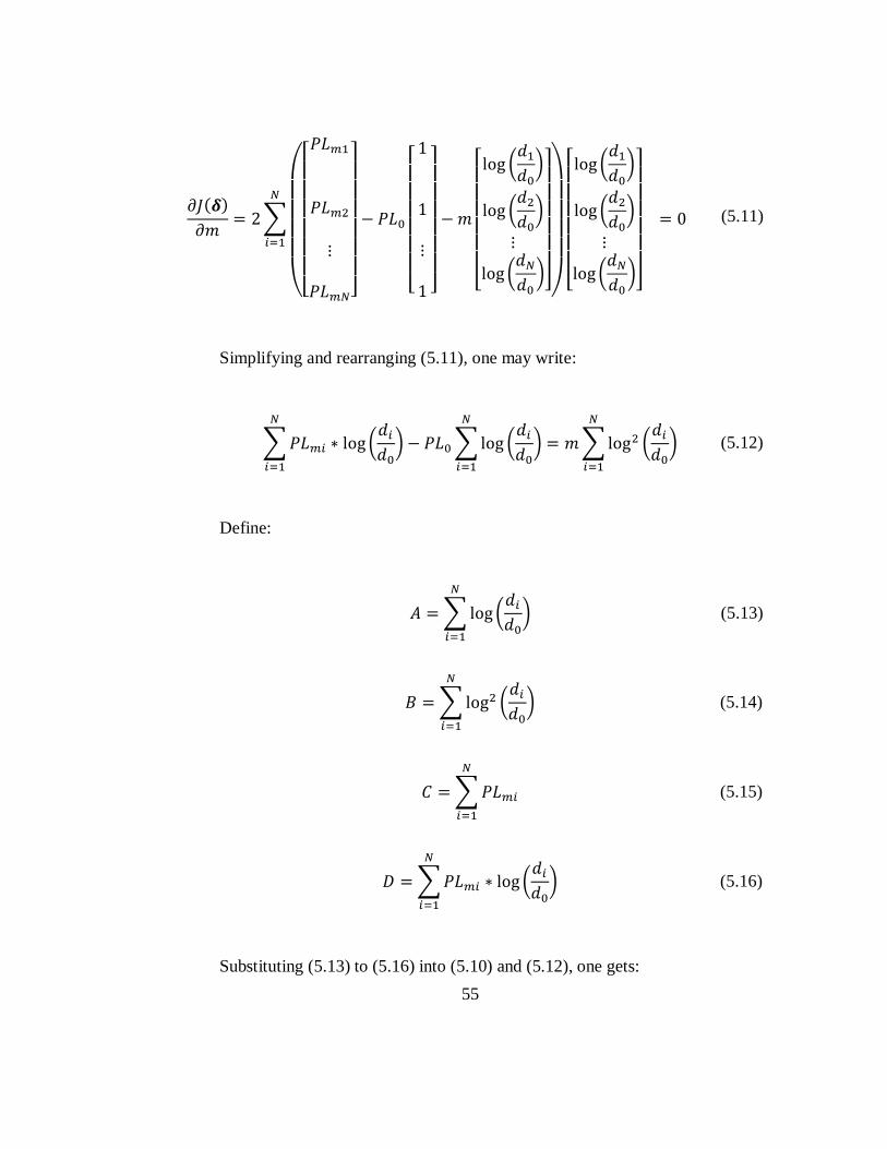
55
𝜕𝐽(𝜹)
𝜕𝑚= 2∑
(
[ 𝑃𝐿𝑚1
𝑃𝐿𝑚2
⋮
𝑃𝐿𝑚𝑁]
− 𝑃𝐿0
[ 1
1
⋮
1 ]
− 𝑚
[ log (
𝑑1𝑑0)
log (𝑑2𝑑0)
⋮
log (𝑑𝑁𝑑0)]
)
[ log (
𝑑1𝑑0)
log (𝑑2𝑑0)
⋮
log (𝑑𝑁𝑑0)]
= 0
𝑁
𝑖=1
(5.11)
Simplifying and rearranging (5.11), one may write:
∑𝑃𝐿𝑚𝑖
𝑁
𝑖=1
∗ log (𝑑𝑖𝑑0) − 𝑃𝐿0∑log (
𝑑𝑖𝑑0)
𝑁
𝑖=1
= 𝑚∑log2 (𝑑𝑖𝑑0)
𝑁
𝑖=1
(5.12)
Define:
𝐴 =∑log(𝑑𝑖𝑑0)
𝑁
𝑖=1
(5.13)
𝐵 =∑log2 (𝑑𝑖𝑑0)
𝑁
𝑖=1
(5.14)
𝐶 =∑𝑃𝐿𝑚𝑖
𝑁
𝑖=1
(5.15)
𝐷 =∑𝑃𝐿𝑚𝑖
𝑁
𝑖=1
∗ log (𝑑𝑖𝑑0) (5.16)
Substituting (5.13) to (5.16) into (5.10) and (5.12), one gets:
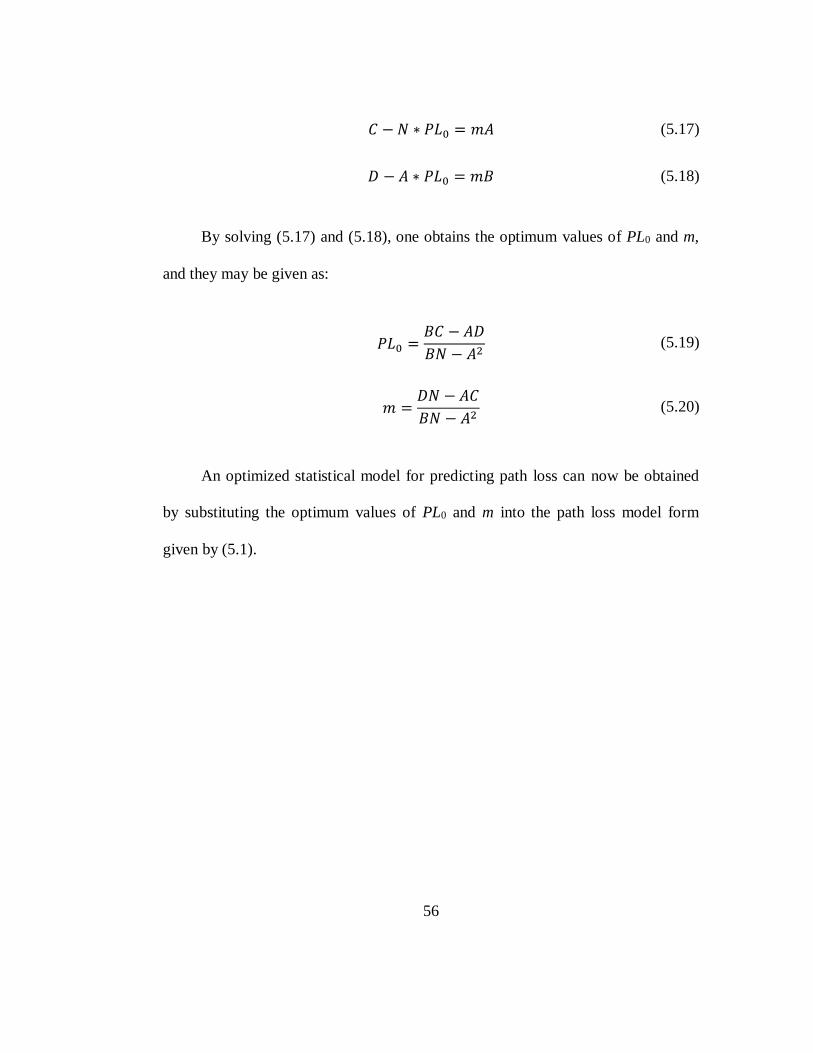
56
𝐶 − 𝑁 ∗ 𝑃𝐿0 = 𝑚𝐴 (5.17)
𝐷 − 𝐴 ∗ 𝑃𝐿0 = 𝑚𝐵 (5.18)
By solving (5.17) and (5.18), one obtains the optimum values of PL0 and m,
and they may be given as:
𝑃𝐿0 =𝐵𝐶 − 𝐴𝐷
𝐵𝑁 − 𝐴2 (5.19)
𝑚 =𝐷𝑁 − 𝐴𝐶
𝐵𝑁 − 𝐴2 (5.20)
An optimized statistical model for predicting path loss can now be obtained
by substituting the optimum values of PL0 and m into the path loss model form
given by (5.1).

57
Chapter 6: Measurement System and
Procedure
6.1 Equipment Description
The measurement system consists of a PCS transmitter, transmit antenna,
receiver, receive antenna, GPS (Global Positioning System) and a laptop with
installed measurement software from Grayson wireless.
6.1.1 Transmitter
The Berkeley Varitronics Systems Transmitter consists of a continuous wave
(CW) generator and power amplifier. This transmitter can be used for measuring
PCS band signal propagation. It covers the frequency range 1.85 to 2.1 GHz. The
transmit power is up to 20 Watt or 43 dBm. The transmitter has a control knob
which is used for adjusting both frequency and power to the desired level. It also
has an LCD screen for displaying frequency, RF power and operating status. Figure
6.1 shows the transmitter used in this work.

58
Figure 6.1: Transmitter
6.1.2 Transmit antenna
The base station antenna which was used in the measurements is presented in
Figure 6.2. This antenna is used to transmit signals in the frequency range from
1850 MHz to 1990 MHz.
Table 6.1 gives the technical specifications of the transmit antenna.
Figure 6.2: Transmit antenna

59
Table 6.1: Transmit antenna technical specifications
Frequency Range
[MHz] Type
Gain
[dBi] Polarization
Length
[cm]
1850-1990 Omni 6 Vertical 90
6.1.3 Antenna Pattern
The antenna pattern describes how the antenna radiates energy into space. In
general, the patterns are specified using two principal patterns: elevation pattern
and azimuth pattern. Whereas the elevation pattern describes the pattern in the
vertical plane, the azimuth pattern refers to the pattern in the horizontal plane. The
patterns are used to determine the antenna gain in a given direction. Based on their
gain pattern the antennas may be classified as: isotropic, directional and omni-
directional. Isotropic antenna radiates energy equally in all directions and it has a
uniform gain. These kind of antennas would have a spherical radiation pattern.
Directional antenna radiates energy more effectively in one or more directions than
in others. Typically, these type of antennas have one main lobe and several minor
lobes. Omni-directional antenna radiates energy uniformly in a certain plane
(circular in shape) with a directional pattern in any other orthogonal plane.
The transmit antenna used in this work is an omni-directional antenna in the
horizontal plane, that is it has a uniform pattern in azimuth plane. This means also
that the transmit antenna has a uniform gain in azimuth (horizontal) direction with

60
directional gain in the elevation (vertical) direction. Figure 6.3 illustrates a plane
cut in a polar coordinates of the azimuth pattern of the antenna used in this work.
The actual antenna gain in the azimuth direction varies between about 6 to 7 dB.
This variation may be neglected and therefore the gain in the azimuth direction is
averaged and it is equal to 6.5 dB.
Figure 6.3: Azimuth antenna pattern in polar coordinates
While the antenna gain is approximately constant in the azimuth plane, it
changes significantly as a function of the elevation. This means that the antenna
gain is a function of the elevation angle between the transmitter and receiver.
2
4
6
8
30
210
60
240
90
270
120
300
150
330
180 0
Actual gain
Average gain

61
Figure 6.4 shows a plane cut of the antenna elevation pattern. The maximum
antenna gain, which occurs in this case at the elevation angle of zero degree, is 6.5
dB. However, for illustrative proposes, the antenna gain is shifted by 30 dB. The
antenna pattern data are provided in the appendix. As can be seen from the
appendix, there are two sets of data for antenna gain in elevation direction are
provided. The average of the two sets was considered as the antenna gain in
elevation direction in this work.
Figure 6.4: Elevation antenna pattern in polar coordinates
10
20
30
40
30
210
60
240
90
270
120
300
150
330
180 0

62
It is sometimes useful to plot the antenna pattern in Cartesian coordinates,
especially when there are several minor lobes (as for the antenna used in this work),
and where the levels of these minor lobes are of special importance. Figure 6.5 re-
illustrates the antenna elevation pattern in the Cartesian coordinates. As seen, the
main lobe of the antenna pattern is between elevation angles (θ) equal to -11 to 11
degrees. However, from practical implementation prospective, the only interesting
part of this lobe is the one that is associated with the negative values of θ.
Figure 6.5: Elevation antenna pattern in Cartesian coordinates
-80 -60 -40 -20 0 20 40 60 80-30
-25
-20
-15
-10
-5
0
5
10
Elevation angle in [degree]
Ante
nna g
ain
in [
dB
]

63
As can be seen from Figure 6.5, the antenna gain drops from its maximum
(6.5 dB) for θ=0 to about -13 dB for θ=-11 degrees. For the considered transmit
antenna in this work, the gain has positive values for θ ranges between 0 and -7
degrees as it is presented in Table 6.2.
Table 6.2: Elevation angle and corresponding antenna gain
θ° 0 -1 -2 -3 -4 -5 -6 -7 -8 -9 -10 -11
Gain [dB] 6.5 6.5 6.4 6 5.7 5 4 2 -0.4 -3.7 -7.9 -13.5
To make sure that antenna pattern effects are considered properly, only
antenna gain values for which θ is between 0 and -11 degrees (main lobe) are
considered. This means that only measurement locations for which the elevation
angle between relay station and base station is smaller than 11 degrees will be
taken into account.
6.1.4 Receiver
Figure 6.6 shows the Grayson Wireless Measurement System receiver which
was used for measuring the received signal level. The receiver is provided with four
inputs. Each input can be connected to a separate antenna. Thus, the receiver has
the ability to process four signals simultaneously. It covers two frequency bands,
i.e. PCS band and cellular band. Whereas input 1 and input 2 are used for receiving

64
PCS band signals, input 3 and input 4 are allocated for cellular band signals. The
corresponding channel bandwidth is 12 kHz and 30 kHz, respectively.
Figure 6.6: Receiver
The frequency range for PCS and cellular bands are 1850-1990 MHz and
824-894 MHz, respectively. Table 6.3 summarizes these values.
Table 6.3: Receiver inputs and their frequency ranges
Antenna Port Receiver Type Frequency range Bandwidth
1 GMR 203N (PCS) 1850-1990 MHz 12 kHz
2 GMR 203N (PCS) 1850-1990 MHz 12 kHz
3 GMR 200 (Cellular) 824-894 MHz 30 kHz
4 GMR 200 (Cellular) 824-894 MHz 30 kHz

65
The receiver is provided with a GPS to determine the coordinates of the point
of interest. Furthermore, the receiver can be connected to a laptop with installed
measurement software to process and analyze the measurements (will be described
in section 6.1.6).
6.1.5 Receive antenna
In this proposal work two receive antennas were used. While the first one
was used to represent the mobile station at certain height level, the other one was
installed at a higher level to simulate the relay station. The two antennas are almost
identical. Both of them have omni-directional pattern and cover the entire PCS
frequency band. The technical specifications for both antennas are summarized in
Table 6.4. Figure 6.7 shows one of the antennas that was used in this work.
Table 6.4: Technical specifications of receive antennas
Antenna scenario
Frequency Range [MHz]
Gain [dBi]
Pattern Whip Length
[inch]
Mount
Diameter
[inch]
Cable
Length
[feet]
Mobile 1850-1990 2.5 Omni 9 3.5 12
Relay 1850-1990 5 Omni 8.5 2.4 15

66
Figure 6.7: Receive antenna
6.1.6 Software
The software that was used to establish the measurements in this work is
called Wireless Measurement System (WMS). It is installed on a laptop and it
consists of a Cellscope and Spectrum tracker software. The software is used to
measure the level of the received signals and map their values on the spectrum
tracker screen along with corresponding frequencies. Much like a spectrum
analyzer, the spectrum tracker maps the frequency on the x-axis [in MHz] and the
signal strength on the y-axis [in dBm]. The spectrum tracker can process up to four
receivers simultaneously. The display reports real time measurements from the
receiver selected in the spectrum tracker submenu. The signal strengths and their
corresponding frequencies can be displayed either numerically or graphically. The
maximum and minimum graphical signal strengths are -45 dBm and -130 dBm,
respectively. Moreover, the software produces a log file for every recording
session. The log file provides a complete reported listing of all of the real time

67
activity. This list includes time, date, frequency, received signal level and receiver
coordinates. Figure 6.8 presents a snapshot of the main menu of the software along
with an example of power measurements at some PCS frequencies. Additionally, it
shows a numerical display of received signal level for some frequencies. Figure 6.9
gives a graphical illustration of RSL for some other frequencies.
Figure 6.8: Power measurements: numerical display

68
Figure 6.9: Power measurements: graphical display
6.2 Receiver Noise Floor and Noise Figure
The noise power at the input of a receiver can be given as
𝑃𝑁 = 𝑘𝑇𝐵 (6.1)
where
k: Boltzmann's constant = 1.379 x10⁻²³ [W/HzK]
T: Absolute temperature in Kelvin [K]
B: Receiver bandwidth in Hertz [Hz]
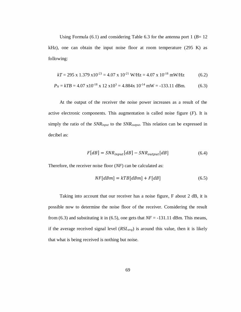
69
Using Formula (6.1) and considering Table 6.3 for the antenna port 1 (B= 12
kHz), one can obtain the input noise floor at room temperature (295 K) as
following:
kT = 295 x 1.379 x10-23 = 4.07 x 10⁻²¹ W/Hz = 4.07 x 10⁻¹⁸ mW/Hz (6.2)
PN = kTB = 4.07 x10-18 x 12 x103 = 4.884x 10⁻¹⁴ mW = -133.11 dBm. (6.3)
At the output of the receiver the noise power increases as a result of the
active electronic components. This augmentation is called noise figure (F). It is
simply the ratio of the SNRinput to the SNRoutput. This relation can be expressed in
decibel as:
𝐹[𝑑𝐵] = 𝑆𝑁𝑅𝑖𝑛𝑝𝑢𝑡[𝑑𝐵] − 𝑆𝑁𝑅𝑜𝑢𝑡𝑝𝑢𝑡[𝑑𝐵] (6.4)
Therefore, the receiver noise floor (NF) can be calculated as:
𝑁𝐹[𝑑𝐵𝑚] = 𝑘𝑇𝐵[𝑑𝐵𝑚] + 𝐹[𝑑𝐵] (6.5)
Taking into account that our receiver has a noise figure, F about 2 dB, it is
possible now to determine the noise floor of the receiver. Considering the result
from (6.3) and substituting it in (6.5), one gets that NF = -131.11 dBm. This means,
if the average received signal level (RSLavg) is around this value, then it is likely
that what is being received is nothing but noise.

70
6.3 Spectrum Clearing
Before conducting the experimental survey, one has to make sure that the
operating frequency used for the path loss measurements is not occupied by any
other applications. In other words, the operating frequency has to be free from any
sources of radiation. Otherwise, the measurements will be corrupted with the
outside interference. This process is called spectrum clearing. In order to achieve
this task, monitoring process for the frequency of interest needs to be established.
The measurement system that has been used for this purpose is illustrated in Figure
6.10, and it consists of the receiver, antenna and laptop with preinstalled software
to measure the received signal level.
Figure 6.10: Spectrum clearing measurement system

71
The antenna was connected to the port 1 to monitor the desired operating
frequency, which is 1925 MHz in this work. The approach here is to ensure that
this frequency is not in use. The monitoring process took place in the Wireless
Center of Excellence (WiCE) lab at Florida Institute of Technology and lasted for
24 hours. The received signal values were recorded as a log file then were
transferred through a macrocode to be presented in a much easier format to work
with.
More than 788,200 measurements were recorded in this test. The signal
strength measurements for the 24 hours test are described by the histogram in
Figure 6.11. It is noticeable that the frequency 1925 MHz is not occupied by any
application. This is because the average measured signal level was around -128
dBm, for about 50 % of the time, which is just noise. Taking into account that the
antenna gain (2.5 dB), and comparing this result to the NF value (-131.11 dBm)
obtained in section 6.2, one finds an excellent match between the theoretical and
the measured value of NF. The figure also shows the normal distribution of the
noise around its mean value with a standard deviation less than 2 dB.

72
Figure 6.11: Signal strength measurements at frequency 1925 MHz for 24 hours
6.4 Procedure
Measurements were conducted by using the equipment described in the
previous sections. The experimental data were collected in outdoor environment
during the daytime. The measurements are conducted over a period of couple of
weeks, with essentially no changes in weather pattern and vegetation. The
measurements conducted for this work are collected in a typical US suburban
environment of Melbourne, FL, USA. Most houses in the selected area were single
to double stories and their heights were about 4 to 9 meters. In general, most of the
buildings are made of wooden structures with exception of few buildings that are
-135 -130 -125 -1200
5
10
15
20
25
30
35
40
45
50
Signal strength in [dBm]
Rela
tive p
erc
enta
ge o
f occure
nce [
%]
Number of measurements = 788,209 mean = -128.23 dBm StDev = 1.85 dB

73
made of combined materials; concrete for frame or body and timber or plastered
bricks for walls, glass for windows, concrete for floors. Few buildings have flat
roofs while most of one story houses and two stories residential apartments have
pitched roofs. The terrain in general is flat with moderate tree densities. Trees
height is up to 13 m.
In this measurement campaign, both the base station transmitter and receiver
were fixed. At transmission side, the antenna was an omni-directional type with 6
dBi gain and vertical polarization. The base station antenna was attached to a mast
and mounted on the top of multi-story building (Crawford Building at Florid
Institute of Technology) as it is shown in Figure 6.12. Therefore, the actual height
of the transmitting antenna is the summation of the height of the building, height of
the mast and half height of the antenna itself. The antenna was then connected to
the transmitter that is generating a continuous wave (CW) signal (un-modulated
single tone carrier). The measurements are collected in 1900MHz band which is
one of the principal bands for the deployment of the LTE and LTE-Advanced. The
transmitted power was set up at 43 dBm.

74
Figure 6.12: Illustration of the base station
At the reception side, data collection process are divided into two campaigns.
First measurement campaign was performed to collect the data for two levels of
receive antenna height, namely 1.7 and 4 meters. Those heights were chosen to
represent the mobile station and relay station, respectively as it is shown in Figure
6.13. The measurement equipment were installed on a cart that can be moved. Two
omni-directional antennas were attached to two plastic masts. Both antennas were
connected to the receiver to measure the received signal strength at the mobile
station and relay station.

75
Figure 6.13: Illustration of the mobile and relay stations
The second measurement campaign was conducted using four different relay
heights ranging from 4 to 16 meters with 4 meter step. The considered heights are
typical where one would find relay deployment in various scenarios. In this
measurement campaign, the receiver was placed in a boom-lift as shown in Figure
6.14 and moved between locations.

76
Figure 6.14: Illustration of the receiver on a boom-lift
At each measurement point, a GPS was used to determine the coordinates of
the receiver. Consequently, the distance from the base station to the receiver can be
calculated. The location of the measurement points in the second campaign is
presented in Figure 6.15.
The parameters associated with the measurements are provided in Table 6.5

77
Figure 6.15: Map of the area where the measurements were conducted. Transmitter
location is – Latitude: 28.064° N, Longitude: 80.624° W
Table 6.5: Parameters associated with the measurement campaign
Parameter Value
Operating frequency 1925 MHz
Tra
nsm
itte
r
Antenna height 25.5 m
Transmitting power 43 dBm
Antenna gain 6 dBi
Cable and connector losses 0.5 dB
Rec
eiv
er
Noise figure 2 dB
Mobile Station
Antenna height 1.7 m
Antenna gain including cable and connector
losses
11.7 dBi
Relay Station
Antenna height 4, 8, 12, 16m
Antenna gain including cable and connector
losses
5 dBi

78
All parameters related to measurements including received signal level,
location of the receiver, date and time were recorded using a laptop with the
software described in section (6.1.6). The measurement system is shown in Figure
6.16.
Figure 6.16: Measurement system
Measurements were conducted at different locations on roads in coverage
area within a region from 100 m to about 4 km from the base station. Whereas for
the first campaign measurements were taken at 155 different locations, 100 of path
loss measurement locations are examined for each relay antenna height in the
second campaign. For each examined antenna height, data were recorded at interval
of 20 ms for about 3-5 minutes. For each measurement location several hundred
readings are averaged in time domain so that the fast-fading component of the

79
signal is smoothed out. Then, the path loss at each location for the different
receiver antenna heights was calculated by using the averaged measured received
signal level.

80
Chapter 7: Path Loss Measurements for
Relay Stations
The main objective of the research described in this chapter is to develop
statistical path loss models for outdoor relaying systems [48, 49]. The path loss
models are derived on a basis of an extensive measurement campaign conducted in
1900 MHz frequency band. The results obtained from the measurements are
presented and discussed in this chapter. Path loss measurements are compared with
path losses predicted using the model given in (5.1). Additionally, the impact of the
relay station antenna height is studied and included in the path loss modeling. An
antenna height correction factor is also derived and included in the modeling.
Finally, a relationship between the intercept, slope of the model and the relay
antenna height is derived.
7.1 Performance Analysis of Path Loss
Measurements
The measured path loss at any given distance (d) from the base station can be
calculated from Eq. (5.3). Recalling the equation:
𝑃𝐿𝑚𝑖 = 𝐸𝑅𝑃 − 𝑃𝑟𝑖 (7.1)

81
Where ERP (Effective Radiated Power) can be calculated as:
𝐸𝑅𝑃 = 𝑃𝑇𝑋 + 𝐺𝑇𝑋 − 𝐶𝐿𝑇𝑋 (7.2)
and Pri (received power at the input of receive antenna) for the ith point can be
calculated as:
𝑃𝑟𝑖 = 𝑅𝑆𝐿𝑖 − 𝐺𝑅𝑋 + 𝐶𝐿𝑅𝑋 (7.3)
Where:
PTX: Transmitted power in dBm
GTX: Gain of transmit antenna in dB
CLTX: Cable losses at transmission side in dB
RSLi: Received Signal Level for the ith point (receiver output) in dBm
GRX: gain of receive antenna in dB
CLRX: Cable losses at reception side in dB
The value of all these parameters were given in Table 6.5 except Pri which
can be obtained from measurements.
Figure 7.1 denotes the geographical location of measurement points of the
first campaign and the location of the base station as well. Additionally, the figure

82
shows the corresponding measured RSL, given by (7.3), at each location for h=4
relay station antenna height.
Figure 7.1: Received signal level by latitude and longitude
The path loss measurements from which the antenna pattern effects have
been taken out are presented in Figure 7.2. Measurements are conducted for 1.7, 4,
8, 12 and 16 m of the receive antenna height. Free space path loss is plotted as well
and as it is seen, it represents a lower boundary for the measurements. The path loss
ranges from about 80 dB to about 180 dB for distances from 100 m to about 4 km.
One can easily observe that the measurements show consistent trends. The increase

83
of path loss is a linear function of the log of distance. The figure shows clearly the
effect of the relay antenna height on the path loss value in which these values
decrease with the increase of relay antenna height. Measurements show less
dependency of path loss value on the relay antenna height when the receiver is
closer to the transmitter. This result may be explained by the fact that in such cases
the receiver and the transmitter are in Line Of Sight (LOS) conditions in which
relay antenna height does not have a significant impact on the received power. On
the other hand, as the distance becomes larger, this dependency is more pronounced
especially at lower relay antenna heights.
Figure 7.2: Measured and predicted path loss for different relay heights
102
103
70
80
90
100
110
120
130
140
150
160
170
180
Distance [m]
Path
Loss [
dB
]
h=1.7 m - Measured
h=1.7 m - Predicted
h=4 m - Measured
h=4 m - Predicted
h=8 m - Measured
h=8 m - Predicted
h=12 m - Measured
h=12 m - Predicted
h=16 m - Measured
h=16 m - Predicted
Free Space

84
The predicted path loss in [dB], solid lines in Figure 7.2, at any given
distance d from the transmitter with respect to a reference distance d0 may be
described as log-distance path loss model and given by:
𝑃𝐿(𝑑) = 𝑃𝐿0 +𝑚 log(𝑑
𝑑0) (7.4)
where 𝑃𝐿0 represents the intercept in [dB] and m is the slope of the model in
[dB/decade]. The intercept PL0 is the path loss value at the reference distance d0.
The optimum values of 𝑃𝐿0 and m were obtained according to the procedure
explained in chapter 5, section 4. In this work, the reference distance d0 was
defined as 100 m.
Table 7.1 summarizes the obtained values of the slope m and intercept 𝑃𝐿0
for different relay antenna heights. As seen, the slope and intercept are functions of
the relay antenna height. For free space, m=20. However, as the path between
transmitter and receiver gets obstructed, m increases. In other words, m increases as
the receive antenna height decreases. It is intuitive that the slope gets closer to the
free space value (m=20) as the relay antenna height is increased. The obtained
values of m are typical according to [35]. Similarly, the intercept PL0 is inversely
proportional to the relay antenna height.
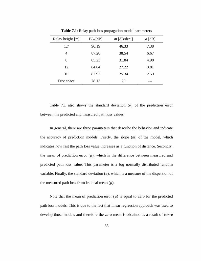
85
Table 7.1: Relay path loss propagation model parameters
Relay height [m] PL0 [dB] m [dB/dec.] σ [dB]
1.7 90.19 46.33 7.38
4 87.28 38.54 6.67
8 85.23 31.84 4.98
12 84.04 27.22 3.81
16 82.93 25.34 2.59
Free space 78.13 20 ---
Table 7.1 also shows the standard deviation (σ) of the prediction error
between the predicted and measured path loss values.
In general, there are three parameters that describe the behavior and indicate
the accuracy of prediction models. Firstly, the slope (m) of the model, which
indicates how fast the path loss value increases as a function of distance. Secondly,
the mean of prediction error (µ), which is the difference between measured and
predicted path loss value. This parameter is a log normally distributed random
variable. Finally, the standard deviation (σ), which is a measure of the dispersion of
the measured path loss from its local mean (µ).
Note that the mean of prediction error (µ) is equal to zero for the predicted
path loss models. This is due to the fact that linear regression approach was used to
develop those models and therefore the zero mean is obtained as a result of curve

86
fitting. More meaningful statistical parameter that describes the reliability of path
loss models is the standard deviation (σ) of the prediction error.
Histograms in Figures 7.3 to 7.7 present the distribution of the prediction
errors about their means for different relay antenna heights. It is observed that
errors are almost log normally distributed about zero means with a standard
deviation that decreases with the increase of the relay antenna height. It is
noteworthy to point out that the variation of the path loss around its mean is due to
the shadowing effect. This variation becomes smaller as the path between the
transmitter and the receiver gets clearer. When the relay antenna height increases,
the received signal experiences less attenuation, reflection or diffraction that caused
by obstacles between transmitter and receiver. Therefore, the standard deviation of
the received signal decreases as the relay antenna increases. The standard deviation,
σ, ranges from 7.38 dB for the antenna height of 1.7 m to 2.59 dB for the highest
relay height (h=16 m). These values of σ are typical for suburban environment in
which the measurements were conducted.

87
Figure 7.3: Distribution of prediction error for h=1.7 m
Figure 7.4: Distribution of prediction error for h=4 m
-20 -16 -12 -8 -4 0 4 8 12 16 200
5
10
15
20
25
Error in [dB]
Rela
tive p
erc
enta
ge o
f occure
nce [
%]
Number of measurements:155 mean =0 dB StDev =7.38 dB
-20 -15 -10 -5 0 5 10 15 200
5
10
15
20
25
Error in [dB]
Rela
tive p
erc
enta
ge o
f occure
nce [
%]
Number of measurements:255 mean =0 dB StDev =6.67 dB
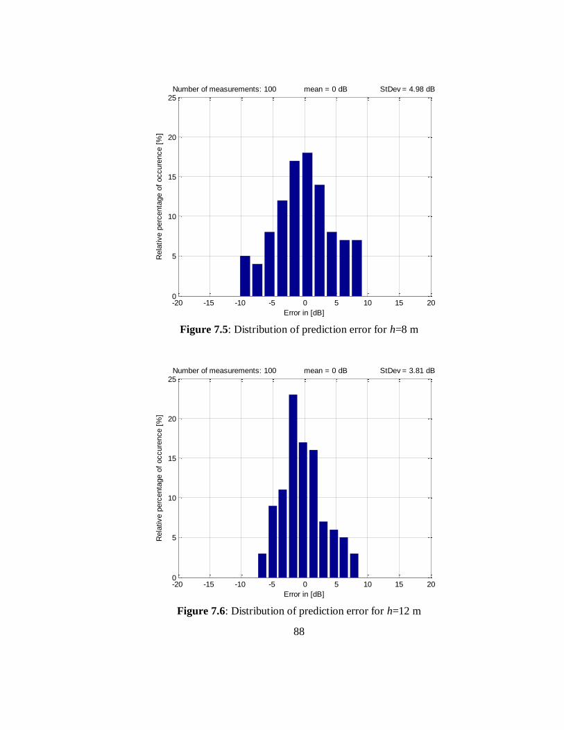
88
Figure 7.5: Distribution of prediction error for h=8 m
Figure 7.6: Distribution of prediction error for h=12 m
-20 -15 -10 -5 0 5 10 15 200
5
10
15
20
25
Error in [dB]
Rela
tive p
erc
enta
ge o
f occure
nce [
%]
Number of measurements: 100 mean = 0 dB StDev = 4.98 dB
-20 -15 -10 -5 0 5 10 15 200
5
10
15
20
25
Error in [dB]
Rela
tive p
erc
enta
ge o
f occure
nce [
%]
Number of measurements: 100 mean = 0 dB StDev = 3.81 dB

89
Figure 7.7: Distribution of prediction error for h=16 m
7.2 Path Loss Models at Different Relay Antenna
Heights
According to the general path loss model given in (7.4) and propagation
model parameters given in Table 7.1, one can write the propagation path loss model
for any of the examined relay antenna heights. For example, in the case of h=1.7 m,
the model is given as:
𝑃𝐿(𝑑) = 90.19 + 46.33 log (𝑑
𝑑0) (7.5)
-20 -15 -10 -5 0 5 10 15 200
5
10
15
20
25
Error in [dB]
Rela
tive p
erc
enta
ge o
f occure
nce [
%]
Number of measurements: 100 mean = 0 dB StDev = 2.59 dB

90
Similar to (7.5), other propagation models for the corresponding relay
antenna heights 4 m, 8 m, 12 m, and 16 m can be expressed as well.
For the case of relay antenna height h=4 m, the model cab be expressed as:
𝑃𝐿(𝑑) = 87.28 + 38.54 log (𝑑
𝑑0) (7.6)
For the case of relay antenna height h=8 m, the model cab be expressed as:
𝑃𝐿(𝑑) = 85.23 + 31.84 log (𝑑
𝑑0) (7.7)
For the case of relay antenna height h=12 m, the model cab be expressed as:
𝑃𝐿(𝑑) = 84.04 + 27.22 log (𝑑
𝑑0) (7.8)
For the case of relay antenna height h=16 m, the model cab be expressed as:
𝑃𝐿(𝑑) = 82.93 + 25.34 log (𝑑
𝑑0) (7.9)
These models are valid for predicting path loss encountered in the relay link
operates in 1900 MHz frequency band and distance ranges from 100-4000 m.
91
7.3 Received Signal Level models for Relay
Stations
Similar to the predicted path loss formula given in (7.4), the predicted
received signal level (RSL) at any given distance d can be obtained as follows:
From (7.1), one may write
𝑅𝑆𝐿(𝑑) = 𝐸𝑅𝑃 − 𝑃𝐿(𝑑) (7.10)
Substituting (7.4) into (7.10), one gets:
𝑅𝑆𝐿(𝑑) = 𝑅𝑆𝐿0 −𝑚log(𝑑
𝑑0) (7.11)
where
𝑅𝑆𝐿0 = 𝐸𝑅𝑃−𝑃𝐿0 (7.12)
where RSL0 in [dBm] is the received signal level at reference distance d0.
Table 7.2 summarizes the obtained values of the slope m and intercept RSL0 for the
examined relay antenna heights.
Note that the values of the slope m and σ for different antenna heights are the
same ones shown in Table 7.1. Comparing Table 7.1 and Table 7.2 one can observe
that while PL0 is decreasing with the increase of receive antenna height, RSL0 is

92
increasing. The predicted and measured received signal level for the examined
relay heights versus distance are plotted in Figure 7.8.
Table 7.2: Relay received signal level parameters
Relay height [m] RSL0 [dBm] m [dB/dec.] σ [dB]
1.7 -41.15 46.33 7.38
4 -38.44 38.54 6.67
8 -36.39 31.84 4.98
12 -35.20 27.22 3.81
16 -34.09 25.34 2.59
Unlike the path loss, received signal level decreases with the increase of
distance. The decrease of received signal level is a linear function of the log of
distance. The figure also shows the impact of relay antenna height on the received
signal values. The obtained results show that higher received signal level is
achieved for higher relay antenna heights.
It is worthy to note that there are two different received antenna with
different gains were used in this work. To show the effect of the relay antenna
height on the received signal level and obtain fair comparison between measured
and predicted values, the increase of the received signal due to antenna gain was
removed. Therefore, the values in Figure 7.8 represent the predicted and measured
received signal level just before the receive antenna.

93
Figure 7.8: Measured and predicted received signal level for different relay heights
Similar to path loss models, received signal level version of propagation
models for the examined relay antenna heights can be presented. According to the
model equation given in (7.11) and the model parameters provided in Table 7.2,
RSL models can be expressed as follows.
For the case of relay antenna height h=1.7 m, the model can be given as:
𝑅𝑆𝐿(𝑑) = −41.15−46.33 log(𝑑
𝑑0) (7.13)
102
103
-140
-120
-100
-80
-60
-40
-20
distance [m]
Receiv
ed S
ignal Level [d
Bm
]
h=1.7 m - Predicted
h=1.7 m - Measured
h=4 m - Predicted
h=4 m - Measured
h=8 m - Predicted
h=8 m - Measured
h=12 m - Predicted
h=12 m - Measured
h=16 m - Predicted
h=16 m - Measured
94
For the case of h=4 m, the model can be written as:
𝑅𝑆𝐿(𝑑) = −38.44−38.54 log(𝑑
𝑑0) (7.14)
For the case of h=8 m, the model can be expressed as:
𝑅𝑆𝐿(𝑑) = −36.39−31.84 log(𝑑
𝑑0) (7.15)
For the case of h=12 m, the model can be given as:
𝑅𝑆𝐿(𝑑) = −35.20−27.22 log(𝑑
𝑑0) (7.16)
For the case of h=16 m, the model can be written as:
𝑅𝑆𝐿(𝑑) = −34.09−25.34 log(𝑑
𝑑0) (7.17)
These models might be used to predict received signal level at relay stations
operating in 1900 MHz band. The models are valid for distances between 100-4000
m from base station.

95
7.4 Path Loss Differences for the Examined Relay
Heights
Studying and analyzing path loss differences between different relay antenna
heights provide general understanding of the impact of relay antenna height on the
path loss values. Additionally, it can be used to derive a correction factor for the
relay antenna height. Consequently, instead of giving a path loss propagation model
for each level of relay antenna height, one is able to derive a general propagation
model that can predict the path loss for a range of relay heights. This can be
achieved by introducing of the relay antenna height correction factor which will be
discussed in the next section.
Table 7.3 shows the average path loss differences quantitatively in terms of
their means and standard deviations for the examined relay antenna heights.
Generally, higher relay antenna height provides smaller path loss. The smallest
average reduction of path loss of 3.21 dB is obtained when the relay antenna height
is changed from 12 to 16 m. Similarly, an average of 18.46 dB path loss difference
is observed when the relay height is raised from 4 to 16 m. The standard deviation
of the path loss differences ranges from 3.59 dB to 8.58 dB. Figure 7.9 to Figure
7.15 illustrate the distributions of the path loss differences for the examined relay
antenna heights.

96
Table 7.3: Average of path loss differences between relay heights
Mean [dB] Standard deviation
[dB]
PL(h=1.7)-PL(h=4) 11.96 8.58
PL(h=4)-PL(h=8) 9.08 6.05
PL(h=8)-PL(h=12) 6.16 4.22
PL(h=4)-PL(h=12) 15.25 7.55
PL(h=12)-PL(h=16) 3.21 3.59
PL(h=8)-PL(h=16) 9.38 5.26
PL(h=4)-PL(h=16) 18.46 8.27
Figure 7.9: Distribution of path loss differences (PL(h=4) - PL(h=8))
-10 -5 0 5 10 15 20 25 30 35 400
5
10
15
20
25
Path loss difference [dB]
Rela
tive o
ccure
nce [
%]
Number of measurements: 100 mean = 9.08 dB StDev = 6.05 dB

97
Figure 7.10: Distribution of path loss differences (PL(h=4) - PL(h=12))
Figure 7.11: Distribution of path loss differences (PL(h=8) - PL(h=12))
-10 -5 0 5 10 15 20 25 30 35 400
5
10
15
20
25
Path loss difference [dB]
Rela
tive o
ccure
nce [
%]
Number of measurements: 100 mean = 15.25 dB StDev = 7.55 dB
-10 -5 0 5 10 15 20 25 30 35 400
5
10
15
20
25
Path loss difference [dB]
Rela
tive o
ccure
nce [
%]
Number of measurements: 100 mean = 6.16 dB StDev = 4.22 dB

98
Figure 7.12: Distribution of path loss differences (PL(h=8) - PL(h=16))
Figure 7.13: Distribution of path loss differences (PL(h=12) - PL(h=16))
-10 -5 0 5 10 15 20 25 30 35 400
5
10
15
20
25
Path loss difference [dB]
Rela
tive o
ccure
nce [
%]
Number of measurements: 100 mean = 9.38 dB StDev = 5.26 dB
-10 -5 0 5 10 15 20 25 30 35 400
5
10
15
20
25
Path loss difference [dB]
Rela
tive o
ccure
nce [
%]
Number of measurements: 100 mean = 3.21 dB StDev = 3.59 dB

99
Figure 7.14: Distribution of path loss differences (PL(h=4) - PL(h=16))
Figure 7.15: Distribution of path loss differences (PL(h=1.7) - PL(h=4))
-10 -5 0 5 10 15 20 25 30 35 400
5
10
15
20
25
Path loss difference [dB]
Rela
tive o
ccure
nce [
%]
Number of measurements: 100 mean = 18.46 dB StDev = 8.27 dB
-10 -5 0 5 10 15 20 25 30 35 400
5
10
15
20
25
Path loss difference [dB]
Rela
tive o
ccure
nce [
%]
Number of measurements: 155 mean =11.96 dB StDev =8.58 dB
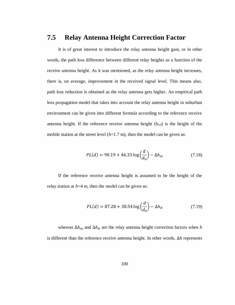
100
7.5 Relay Antenna Height Correction Factor
It is of great interest to introduce the relay antenna height gain, or in other
words, the path loss difference between different relay heights as a function of the
receive antenna height. As it was mentioned, as the relay antenna height increases,
there is, on average, improvement in the received signal level. This means also,
path loss reduction is obtained as the relay antenna gets higher. An empirical path
loss propagation model that takes into account the relay antenna height in suburban
environment can be given into different formula according to the reference receive
antenna height. If the reference receive antenna height (href) is the height of the
mobile station at the street level (h=1.7 m), then the model can be given as:
𝑃𝐿(𝑑) = 90.19 + 46.33 log (𝑑
𝑑0) − ∆ℎ𝑚 (7.18)
If the reference receive antenna height is assumed to be the height of the
relay station at h=4 m, then the model can be given as:
𝑃𝐿(𝑑) = 87.28 + 38.54 log (𝑑
𝑑0) − ∆ℎ𝑅 (7.19)
whereas ∆ℎ𝑚 and ∆ℎ𝑅 are the relay antenna height correction factors when h
is different than the reference receive antenna height. In other words, Δℎ represents

101
the reduction of the path loss, or the improvement in the received signal level, as
the result of the relay antenna height increase.
Based on Table 7.3, the average relay antenna height correction factor ∆ℎ𝑚
and ∆ℎ𝑅 may be approximated as:
∆ℎ̅̅̅̅ 𝑚[dB] = 31.44 log (ℎ
1.7) (7.20)
and
∆ℎ̅̅̅̅ 𝑅[dB] = 31.1 log (ℎ
4) (7.21)
for reference receive antenna height h=1.7 m and h=4 m, respectively.
Equations (7.20) and (7.21) are based on the trends of the empirical relationship
between the path loss differences as a function of the relay antenna height as
provided in Table 7.3. These relationships along with the trend lines are graphically
illustrated in Figure 7.16 and Figure 7.17. As can be seen from these figures, the
trend line equations given in (7.20) and (7.21) show a very good fit with the
measured path loss differences for the examined relay antenna heights.
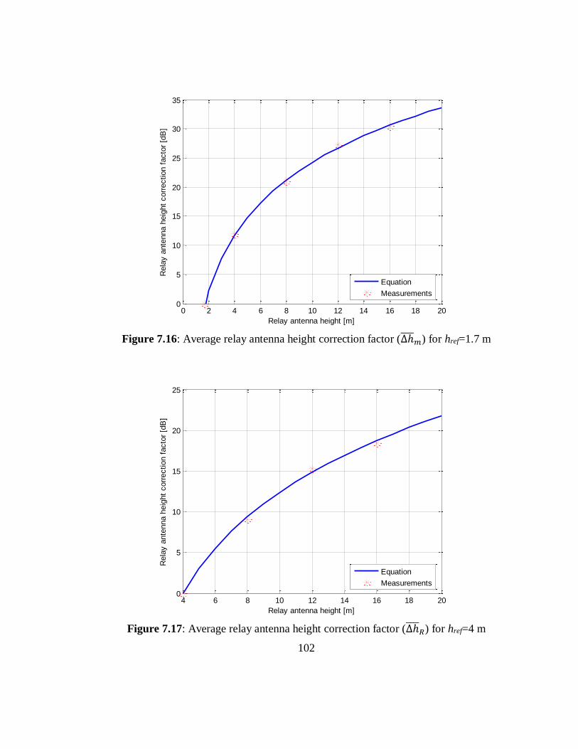
102
Figure 7.16: Average relay antenna height correction factor (∆ℎ̅̅̅̅ 𝑚) for href=1.7 m
Figure 7.17: Average relay antenna height correction factor (∆ℎ̅̅̅̅ 𝑅) for href=4 m
0 2 4 6 8 10 12 14 16 18 200
5
10
15
20
25
30
35
Relay antenna height [m]
Rela
y a
nte
nna h
eig
ht
corr
ection f
acto
r [d
B]
Equation
Measurements
4 6 8 10 12 14 16 18 200
5
10
15
20
25
Relay antenna height [m]
Rela
y a
nte
nna h
eig
ht
corr
ection f
acto
r [d
B]
Equation
Measurements
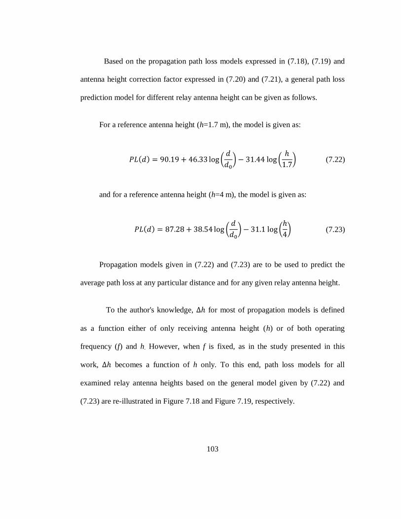
103
Based on the propagation path loss models expressed in (7.18), (7.19) and
antenna height correction factor expressed in (7.20) and (7.21), a general path loss
prediction model for different relay antenna height can be given as follows.
For a reference antenna height (h=1.7 m), the model is given as:
𝑃𝐿(𝑑) = 90.19 + 46.33 log (𝑑
𝑑0) − 31.44 log (
ℎ
1.7) (7.22)
and for a reference antenna height (h=4 m), the model is given as:
𝑃𝐿(𝑑) = 87.28 + 38.54 log (𝑑
𝑑0) − 31.1 log (
ℎ
4) (7.23)
Propagation models given in (7.22) and (7.23) are to be used to predict the
average path loss at any particular distance and for any given relay antenna height.
To the author's knowledge, Δℎ for most of propagation models is defined
as a function either of only receiving antenna height (h) or of both operating
frequency (f) and h. However, when f is fixed, as in the study presented in this
work, Δℎ becomes a function of h only. To this end, path loss models for all
examined relay antenna heights based on the general model given by (7.22) and
(7.23) are re-illustrated in Figure 7.18 and Figure 7.19, respectively.

104
As cab be seen from the figures, path loss difference between any two relay
antenna heights is now constant for the entire distance range. Some observations
can be drawn from these figures. Firstly, it is observed that the obtained predicted
path loss values for relay antenna heights different than the reference height are
different from the actual path loss (compare to measurements in Figure 7.2).
Secondly, model predictions seem to be very optimistic when the relay station is
close to the base station. Some of them even show less path loss values than the
free space model which is not realistic.
Figure 7.18: Path loss models based on the average relay antenna height correction
factor for href=1.7 m
102
103
60
70
80
90
100
110
120
130
140
150
160
Distance [m]
Path
Loss [
dB
]
h=1.7 m - Predicted
h=4 m - Predicted
h=8 m - Predicted
h=12 m - Predicted
h=16 m - Predicted
Free Space

105
Figure 7.19: Path loss models based on the average relay antenna height correction
factor for href=4 m
Additionally, the models overestimate the predicted path loss when the relay
station is far from the base station. Finally, the intercept (PL0) and slope (m) of
these models are also different from that obtained from measurements and
summarized in Table 7.1.
For more illustrations, Figure 7.20 presents the error between the actual
model predictions and the ones that are based on the implementation of the average
relay antenna height correction factor for href=1.7 m.
102
103
60
70
80
90
100
110
120
130
140
150
160
Distance [m]
Path
Loss [
dB
]
h=4 m - Predicted
h=1.7 m - Predicted
h=8 m - Predicted
h=12 m - Predicted
h=16 m - Predicted
Free Space

106
Figure 7.20: Prediction error based on the average relay antenna height correction
factor (∆ℎ̅̅̅̅ 𝑚) for href=1.7 m
From Figure 7.20, one can see that the implementation of the average relay
antenna height results in tolerant errors only when the distance is between about
1000 m and 1500 m. In this range, the error is less than 2 dB. However, for smaller
and larger distances, the error increases rapidly especially for high relay antenna
heights. It is noteworthy to mention that positive value of the error means that the
model underestimates the actual path loss value. On the contrary, negative values
indicate that the model over predicts the path loss.
500 1000 1500 2000 2500 3000 3500 4000-15
-10
-5
0
5
10
15
20
25
Distance [m]
Err
or
[dB
]
h=1.7 m
h=4 m
h=8 m
h=12 m
h=16 m
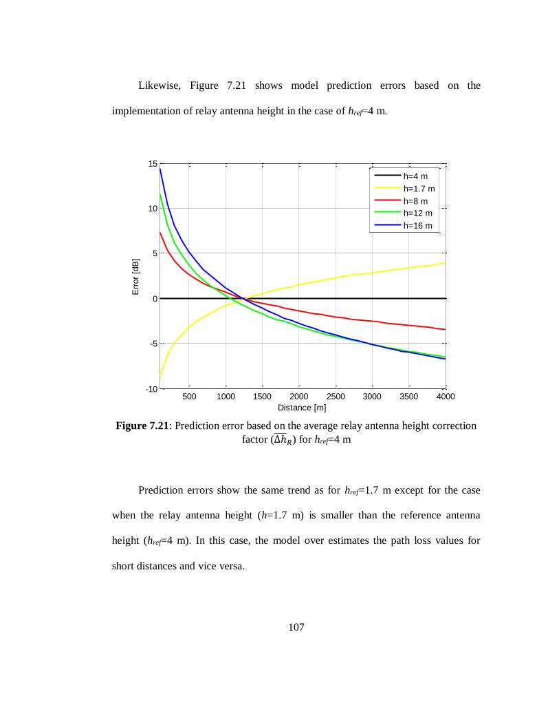
107
Likewise, Figure 7.21 shows model prediction errors based on the
implementation of relay antenna height in the case of href=4 m.
Figure 7.21: Prediction error based on the average relay antenna height correction
factor (∆ℎ̅̅̅̅ 𝑅) for href=4 m
Prediction errors show the same trend as for href=1.7 m except for the case
when the relay antenna height (h=1.7 m) is smaller than the reference antenna
height (href=4 m). In this case, the model over estimates the path loss values for
short distances and vice versa.
500 1000 1500 2000 2500 3000 3500 4000-10
-5
0
5
10
15
Distance [m]
Err
or
[dB
]
h=4 m
h=1.7 m
h=8 m
h=12 m
h=16 m

108
From Figure 7.20 and Figure 7.21, it is clear that the implementation of the
average relay antenna height correction factors given in (7.20) and (7.21) which
take only the relay height into consideration is not the appropriate approach to
develop a general empirical path loss propagation model. This is because of the
large obtained prediction errors as a result of this approach.
From the previous discussion, it is obvious that one or more parameters need
to be taken into account when evaluating Δℎ. Measurements show, as it was
presented in Figure 7.2, that Δℎ is not only a function of relay antenna height (h)
but it is also a linear function of the log of distance (d).
To understand and derive the relationship between Δℎ and distance,
following simple scenario is considered. According to the measurements (refer to
Figure 7.2), any two path loss models that have different relay antenna height h1
and h2, models might be given as:
𝑃𝐿1,2(𝑑) = 𝑃𝐿01,02 +𝑚1,2 log (𝑑
𝑑0) (7.24)
where ℎ1 > ℎ2, 𝑚1 < 𝑚2, 𝑃𝐿01 < 𝑃𝐿02.
Figure 7.22 illustrates the models expressed in (7.24).

109
Distance
h1
h2
m1
m2Δh
PL01
PL02
Pat
h l
oss
[dB
]
Figure 7.22: Illustration of Δℎ as a function of relay height and distance
As can be seen from Figure 7.22, the antenna height correction factor Δℎ is
no longer constant between any two particular path loss models as it was shown in
Figure 7.18 and Figure 7.19. Δℎ, however, increases as a linear function of the log
of distance d. The path loss difference ΔPL at any particular distance for two
different antenna heights which is also equal to Δℎ can be given as:
∆𝑃𝐿 = ∆ℎ = 𝑥log(ℎ1ℎ2) = ∆𝑃𝐿0 + ∆𝑚 log(
𝑑
𝑑0) (7.25)
where ∆𝑃𝐿0 = 𝑃𝐿02 − 𝑃𝐿01, ∆𝑚 = 𝑚2 −𝑚1 and x is the slope of the
antenna height dependence that needs to be determined.

110
To generalize the expression given in (7.25), h2 will be considered as href and
h1 can be any value of the examined relay antenna heights (h). Therefore, the value
of x may be calculated as:
𝑥[dB] =∆𝑚 log(
𝑑𝑑0) + ∆𝑃𝐿0
log (ℎℎ𝑟𝑒𝑓
) (7.26)
Two reference antenna heights will be considered for the derivation of the
antenna height correction factor ∆ℎ. Note that the goal of determining ∆ℎ is to find
a general path loss model that can be used for any relay antenna height relative to a
reference antenna height. The two reference antenna heights are href=4 m and
href=1.7 m. Table 7.4 and Table 7.5 show the values of ∆𝑚 and ∆𝑃𝐿0 for the
examined relay heights in the cases of href=4 m and href=1.7 m, respectively.
Table 7.4: Slope and intercept differences for href =4 m
h [m] 𝑃𝐿0 [dB] ∆𝑃𝐿0 [dB] 𝑚 [dB/dec] ∆𝑚 [dB/dec]
1.7 90.19 -2.91 46.33 -7.79
4 87.28 0 38.54 0
8 85.23 2.05 31.84 6.7
12 84.04 3.24 27.22 11.32
16 82.93 4.35 25.34 13.2

111
Table 7.5: Slope and intercept differences for href =1.7 m
h [m] 𝑃𝐿0 [dB] ∆𝑃𝐿0 [dB] 𝑚 [dB/dec] ∆𝑚 [dB/dec]
1.7 90.19 0 46.33 0
4 87.28 2.91 38.54 7.79
8 85.23 4.96 31.84 14.49
12 84.04 6.15 27.22 19.11
16 82.93 7.26 25.34 20.99
Now, the task is to find the value of x that was expressed in (7.26) for all
examined relay heights (h) for the two reference cases.
7.5.1 For the case href=4 m:
Considering (7.26) and Table 7.4, x for different relay heights can be given
as:
For h=1.7 m
𝑥[dB] = 20.96 log (𝑑
𝑑0) + 7.83 (7.27)
For h=8 m
𝑥[dB] = 22.26 log (𝑑
𝑑0) + 6.81 (7.28)

112
For h=12 m
𝑥[dB] = 23.72 log (𝑑
𝑑0) + 6.79 (7.29)
For h=16 m
𝑥[dB] = 21.92 log (𝑑
𝑑0) + 7.23 (7.30)
To find the value of x that might be used for different relay heights, it turns
out that taking the average of x is the appropriate approach to determine this value.
Thus, the mean value of x is given by:
𝑥[dB] = 22.21 log (𝑑
𝑑0) + 7.17 (7.31)
By substituting (7.31) into (7.25), the antenna height correction factor is now
can be given as:
∆ℎ = [22.21 log (𝑑
𝑑0) + 7.17] log (
ℎ
4) (7.32)
Equation (7.32) has two coefficients, 22.21 and 7.17, that are dependent on
the environment. ∆ℎ is illustrated graphically in Figure 7.23. This figure presents a
family of curves of ∆ℎ as a function of distance (d) for different relay antenna

113
heights (h). The figure clearly shows the dependency of ∆ℎ on the distance between
the transmitter and the relay station. This dependency is especially pronounced for
high relay heights. For instance, in the case h=16 m, ∆ℎ increases from less than 5
dB at d=100 m to about 26 dB at d=4000 m. Even though the increase in ∆ℎ is
relatively smaller (from about 1 dB to 7.5 dB) in the case of h=6 m, the changes in
∆ℎ confirms that ∆ℎ is not only function of relay height (h) but also function of
distance.
Figure 7.23: Relay antenna height correction factor (∆ℎ) as a funtion of distance
and relay height
500 1000 1500 2000 2500 3000 3500 40000
5
10
15
20
25
30
Distance [m]
Rela
y a
nte
nna h
eig
ht
corr
ection f
acto
r [d
B]
h=16 m
h=14 m
h=12 m
h=10 m
h=8 m
h=6 m

114
Thus, (7.32) and Figure 7.23 help explain how it is very important to take
into account the distance dependency when considering the relay antenna height
correction factor. This dependency has a great effect on the predicted path loss
value and therefore on the model accuracy. Lack of this consideration might lead to
very large errors in path loss predictions as it was explained earlier.
Note that the goal of finding an empirical path loss model that takes into
account the relay antenna height correction factor has been achieved. This model is
expressed as:
𝑃𝐿(𝑑) = 87.28 + 38.54 log (𝑑
𝑑0) − ∆ℎ (7.33)
where ∆ℎ is given as in (7.32).
To verify the validity of the path loss model proposed in (7.33) after the
implementation of ∆ℎ, a comparison between the model predictions and the
measurements is shown in Figure 7.24.
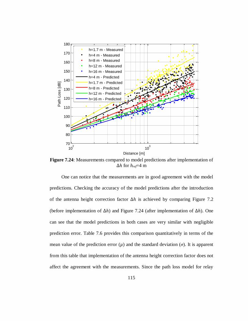
115
Figure 7.24: Measurements compared to model predictions after implementation of
∆ℎ for href=4 m
One can notice that the measurements are in good agreement with the model
predictions. Checking the accuracy of the model predictions after the introduction
of the antenna height correction factor ∆ℎ is achieved by comparing Figure 7.2
(before implementation of ∆ℎ) and Figure 7.24 (after implementation of ∆ℎ). One
can see that the model predictions in both cases are very similar with negligible
prediction error. Table 7.6 provides this comparison quantitatively in terms of the
mean value of the prediction error (µ) and the standard deviation (σ). It is apparent
from this table that implementation of the antenna height correction factor does not
affect the agreement with the measurements. Since the path loss model for relay
102
103
70
80
90
100
110
120
130
140
150
160
170
180
Distance [m]
Path
Loss [
dB
]
h=1.7 m - Measured
h=4 m - Measured
h=8 m - Measured
h=12 m - Measured
h=16 m - Measured
h=4 m - Predicted
h=1.7 m - Predicted
h=8 m - Predicted
h=12 m - Predicted
h=16 m - Predicted

116
height equal to 4 m was taken as a reference for other models, there is no change in
its µ and σ before and after implementation of antenna height correction factor.
Table 7.6: Model comparison before and after implementation of ∆𝒉 relative to the
measurements for href=4 m
h [m] Mean µ [dB] Standard deviation σ [dB]
Before After Before After
1.7 0 0.30 7.38 7.38
4 0 0 6.67 6.67
8 0 0.04 4.98 4.66
12 0 0.78 3.81 3.43
16 0 0.15 2.59 2.23
After the determination of the relay antenna height correction factor, it is of
great interest to show how the slope (m) and the intercept (PL0) of relay path loss
propagation model change with the relay height. To derive the relationship between
the model parameters (m and PL0) and the relay height (h), (7.33) is to be
reconsidered. Rewriting (7.33) with the associated ∆ℎ given in (7.32), one may get:
𝑃𝐿(𝑑) = 87.28 + 38.54 log (𝑑
𝑑0)
− 22.21 log (𝑑
𝑑0) log (
ℎ
4) − 7.17 log (
ℎ
4)
(7.34)
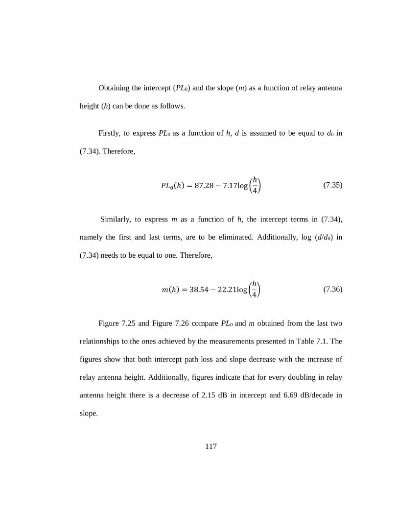
117
Obtaining the intercept (PL0) and the slope (m) as a function of relay antenna
height (h) can be done as follows.
Firstly, to express PL0 as a function of h, d is assumed to be equal to d0 in
(7.34). Therefore,
𝑃𝐿0(ℎ) = 87.28 − 7.17log (ℎ
4) (7.35)
Similarly, to express m as a function of h, the intercept terms in (7.34),
namely the first and last terms, are to be eliminated. Additionally, log (d/d0) in
(7.34) needs to be equal to one. Therefore,
𝑚(ℎ) = 38.54 − 22.21log (ℎ
4) (7.36)
Figure 7.25 and Figure 7.26 compare PL0 and m obtained from the last two
relationships to the ones achieved by the measurements presented in Table 7.1. The
figures show that both intercept path loss and slope decrease with the increase of
relay antenna height. Additionally, figures indicate that for every doubling in relay
antenna height there is a decrease of 2.15 dB in intercept and 6.69 dB/decade in
slope.
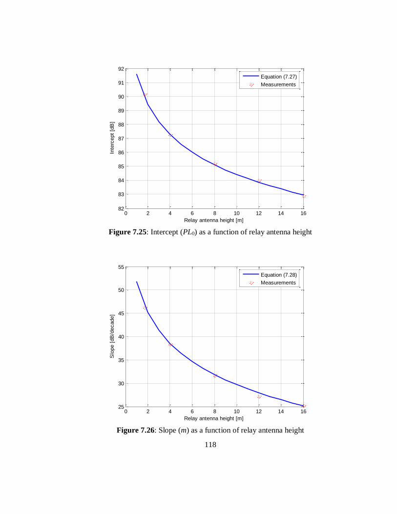
118
Figure 7.25: Intercept (PL0) as a function of relay antenna height
Figure 7.26: Slope (m) as a function of relay antenna height
0 2 4 6 8 10 12 14 1682
83
84
85
86
87
88
89
90
91
92
Relay antenna height [m]
Inte
rcept
[dB
]
Equation (7.27)
Measurements
0 2 4 6 8 10 12 14 1625
30
35
40
45
50
55
Relay antenna height [m]
Slo
pe [
dB
/decade]
Equation (7.28)
Measurements

119
Formulas given in (7.35) and (7.36) represent mathematical expressions by
which one can calculate the intercept (PL0) and slope (m) for any given relay
antenna height ranging from 2 to 16 m.
Thus, another approach of developing empirical propagation path loss models
for relay environment has been achieved. This model might be given as:
𝑃𝐿(𝑑) = 𝑃𝐿0(ℎ) +𝑚(ℎ) log (𝑑
𝑑0) (7.37)
where 𝑃𝐿0(ℎ) and 𝑚(ℎ) can be calculated by (7.35) and (7.36), respectively.
To prove the validity of the model given in (7.37), a comparison between
model predictions and measurements is made in Table 7.7.
Table 7.7: Comparison between measurements and model predictions
h [m]
Measurements Model predictions
𝑃𝐿0 [dB]
𝑚 [dB/dec]
µ
[dB]
σ
[dB] 𝑃𝐿0 [dB]
𝑚 [dB/dec]
µ
[dB]
σ
[dB]
1.7 90.19 46.33 0 7.38 89.94 46.79 0.30 7.38
4 87.28 38.54 0 6.67 87.28 38.54 0 6.67
8 85.23 31.84 0 4.98 85.12 31.85 0.04 4.66
12 84.04 27.22 0 3.81 83.86 27.94 0.78 3.43
16 82.93 25.34 0 2.59 82.96 25.17 0.15 2.23

120
As may be seen from Table 7.7, model predictions and model parameters are
in good agreement with the ones that obtained by the measurements. Therefore, the
statistical propagation model expressed in (7.37) with its associated parameters
𝑃𝐿0(ℎ) and 𝑚(ℎ) given in (7.35) and (7.36) may be used to predict the path loss at
any particular distance for relaying scenarios in suburban areas.
7.5.2 For the case href=1.7 m:
Considering (7.26) and Table 7.5, x for different relay heights can be given
as:
For h=4 m
𝑥[dB] = 20.96 log (𝑑
𝑑0) + 7.83 (7.38)
For h=8 m
𝑥[dB] = 21.54 log (𝑑
𝑑0) + 7.37 (7.39)
For h=12 m
𝑥[dB] = 22.52 log (𝑑
𝑑0) + 7.23 (7.40)
For h=16 m

121
𝑥[dB] = 21.56 log (𝑑
𝑑0) + 7.46 (7.41)
With the same approach followed in the previous case (href=4 m), the average
value of x might be given as:
𝑥[dB] = 21.65 log (𝑑
𝑑0) + 7.48 (7.42)
To find ∆ℎ for the case of href=1.7 m, one needs to substitute (7.42) into
(7.25). Therefore,
∆ℎ = [21.65 log (𝑑
𝑑0) + 7.48] log (
ℎ
1.7) (7.43)
Taking ∆ℎ into account, the empirical path loss model when reference
antenna height is equal to 1.7 m is given as:
𝑃𝐿(𝑑) = 90.19 + 46.33 log (𝑑
𝑑0) − ∆ℎ (7.44)
where ∆ℎ is given as in (7.43).
If one were to plot path loss curves using (7.36) for h= 1.7, 4, 8, 12 or 16
meter, one would obtain similar curves to those presented in Figure 7.2 with
negligible error.

122
Table 7.8 provides a comparison between the models before and after
implementing the antenna height correction factor relative to the measurements.
Ones again, it is clear from the table that implementation of ∆ℎ has no effect on the
agreement with the measurements.
Table 7.8: Model comparison before and after implementation of ∆h relative to the
measurements for href=1.7 m
h [m] Mean µ [dB] Standard deviation σ [dB]
Before After Before After
1.7 0 0 7.38 7.38
4 0 -0.16 6.67 6.67
8 0 -0.02 4.98 4.66
12 0 0.78 3.81 3.43
16 0 0.18 2.59 2.24
From the results in Table 7.6 and Table 7.8, it turns out that regardless of
which one of reference antenna heights (href=1.7 or 4 m) is used, path loss models
proposed in (7.33) and (7.44) can perform with approximately the same accuracy.
Therefore, those proposed models along with the associated Δℎ present general
propagation models. Either one of those models might be used to predict the path
loss value at any particular distance for any given relay station antenna height
between 4 m and 16 m which is a suitable range of relay antenna height and within
environment similar to one surveyed in the measurement campaign.

123
Chapter 8: Developed Path Loss Models
for Relaying Systems
In chapter 4, a number of propagation models were discussed. They can be
grouped by their applicability in relaying systems. While the models in the first
group, namely 3GPP model, WINNER B5f model and IEEE802.16j model were
specifically developed for relaying deployment, the models in the other group were
not. However, because they are widely used propagation models for planning
cellular networks, it is of great interest to establish a relationship between
measurements and some of these standard propagation models. Well known
examples of those models are Lee model and COST231-Hata model. In this
chapter, the validity of the above mentioned models is evaluated by comparing
their performance with measurements [48-50]. Note that the evaluation is limited to
the prediction of path loss encountered on the backhaul link only. Additionally,
some modifications of the original forms of the discussed models are introduced to
make their predictions more reliable in relay environments.
8.1 Performance Analysis of Existing Models
The validity of existing propagation models is examined by comparing their
path loss predictions to the measurements. Each individual propagation model has

124
its own set of assumptions and is restricted to a specific range of parameters under
which it was derived.
8.1.1 Corresponding Assumptions for Considered
Models
For each propagation model, the following assumptions are considered when
those models are used to predict path loss. More information about these models
are available in chapter 4.
For the case of 3GPP model, NLOS condition was assumed since the link
between the base station and the relay station (backhaul link) was obstructed by
buildings and trees at most of the measurement locations. The model is given by
[8]:
𝑃𝐿3GPP[dB] = 125.2 + 36.3 log(𝑑) (8.1)
where d in [km] is the eNodeB-relay separation.
Among the proposed models by WINNER II is the WINNER B5f which is
the most appropriate model for the prediction of the path loss on a backhaul link.
WINNER B5f model takes into account both LOS and NLOS conditions where the
eNodeB antenna height is above the rooftop level and the relay station antenna
height is either above or below the rooftop level. WINNER B5f model is given by
[14]:

125
𝑃𝐿WINNER B5f[dB] = 57.5 + 23.5 log(𝑑) + 23log (𝑓
5) (8.2)
where d in [m] is the distance and f in [GHz] is the frequency.
In the case of IEEE802.16j model [15], terrain type "B" with constants a =
4.0 , b = 0.0065 and c = 17.1 was considered as the most suitable one for the
environment in which the measurements were collected. The general model
formula is given as:
𝑃𝐿IEEE802.16j[dB] = 𝐴 + 10γlog(𝑑
𝑑0) + ∆𝑃𝐿𝑓 + ∆𝑃𝐿ℎ (8.3)
where the model parameters were already defined in section 4.3.3.5.
Note that for the case of COST231-Hata model, "suburban environment"
category with receive antenna height correction factor a (hm) for small to medium
city was used. COST231-Hata model equation is given by [44]:
𝑃𝐿COST231−Hata[dB] = 𝐴 + 𝐵log(𝑑) + 𝐶𝑚 + 𝑎(ℎ𝑚) (8.4)
where A, B, d, Cm and a (hm) were defined in section 4.3.3.4.
For the case of Lee model, corresponding values of slope and intercept for
"suburban area" were assumed. The model is provided relative to reference
conditions and is given as [41]:

126
𝑃𝐿Lee = 𝑃𝐿0 +𝑚log(𝑑
𝑑0) − 15log(
ℎ𝑡ℎ𝑡𝑟𝑒𝑓
) − 10log(ℎ𝑟ℎ𝑟𝑟𝑒𝑓
) (8.5)
where all Lee model parameters were defined in section 4.3.3.2.
Finally, for the new relay model proposed in [21], there are no assumptions to
consider and therefore the model is given as:
𝑃𝐿Relay model[dB] = 34 log(𝑑) + 5 + 26log (20− ℎ𝑅𝑆) (8.6)
where hRS in [m] is the relay antenna height.
8.1.2 Simplified Versions of Existing Models
In the following, each individual propagation model performance relative to
the measurements is discussed. To make the comparison more explicatory, each
propagation model is expressed in a simplified form. In other words, model
equations given by (8.1) - (8.6) are simplified into a general path loss model
formula that is given as:
𝑃𝐿[dB] = 𝑃𝐿0 +𝑚log(𝑑
𝑑0) + ∆ℎ (8.7)
where PL0 is the path loss value at d0=100 m, m is the slope, d is the distance
in meters and Δh in decibel is the relay antenna height correction factor which
allows to predict path loss for different relay heights. To express each model in the

127
simplified form given by (8.7), all models' parameters are replaced with their actual
values. Corresponding parameters values for the considered models are
summarized in Table 8.1.
Table 8.1: Models parameters assumptions for measurement campaign
Model Parameter Value
All models
Frequency 1925 MHz
Transmit antenna
height 25.5 m
Receive antenna
height 4, 8, 12, 16 m
IEEE802.16j Terrain type B a=4, b=0.0065, c=17.1
COST231-Hata
Environment suburban
a (hm) Eq. (4.15)
Cm 0 dB
Lee
m 38.4 dB/dec
PL0 @ f=1925 MHz 114.3 dB
htref 30.48 m
hrref 3.048 m
3GPP NA NA
WINNER B5f NA NA
Relay model [21] NA NA

128
Regarding Lee model, note that PL0 at f=1925 MHz was calculated according
to Table 4.3 and Eq. (4.13). After substituting of all parameters values in equations
(8.1) to (8.6), each individual simplified model formula is now can be determined.
Note that for all considered propagation models the relay antenna height in [m] is
replaced with the parameter h. Additionally, parameter ''d'' is expressed in meters
for all models. After these basic adjustments, the model equations become as
follows.
For 3GPP model:
𝑃𝐿3𝐺𝑃𝑃[dB] = 88.9 + 36.3 log (𝑑
𝑑0) + ∆ℎ3𝐺𝑃𝑃 (8.8)
where Δh3GPP=0.
For WINNER B5f model:
𝑃𝐿𝑊𝐼𝑁𝑁𝐸𝑅 𝐵5𝑓[dB] = 94.97 + 23.5 log (𝑑
𝑑0) + ∆ℎ𝑊𝐼𝑁𝑁𝐸𝑅 𝐵5𝑓 (8.9)
where ΔhWINNER B5f=0.
For IEEE802.16j model:
𝑃𝐿𝐼𝐸𝐸𝐸802.16𝑗[dB] = 78.07 + 45 log (𝑑
𝑑0) − 11.12 log (
ℎ𝑟3) (8.10)

129
For COST231-Hata model:
𝑃𝐿𝐶𝑂𝑆𝑇231−𝐻𝑎𝑡𝑎[dB] = 106.83 + 35.69 log (𝑑
𝑑0) − 2.91ℎ𝑟 (8.11)
For Lee model:
𝑃𝐿𝐿𝑒𝑒[dB] = 73.97 + 38.4 log (𝑑
𝑑0) − 10log(ℎ𝑟) (8.12)
For relay model [21]:
𝑃𝐿𝑅𝑒𝑙𝑎𝑦 𝑚𝑜𝑑𝑒𝑙[dB] = 73 + 34 log(𝑑
𝑑0) + 26log (20 − ℎ𝑅𝑆) (8.13)
It is worth noting that equations (8.8) to (8.13) represent just a simplified
versions of the original forms of models without any further modifications. As far
as the performance of the considered models is concerned, a number of
observations can be pointed out. As can be seen from the previous model equations,
the slope (m) of each individual model is constant and does not depend on relay
antenna height. Furthermore, it is apparent that relay model, COST-Hata, 3GPP,
Lee models exhibit similar slope values, namely, 34, 35.69, 36.3 and 38.4 dB/dec,
respectively which are closer to the ones obtained from the measurements
presented in the previous chapter. On the contrary, WINNER B5f and IEEE802.16j
models manifest completely different slopes. While for WINNER B5f model

130
m=23.5 is relatively small compared to the measurements, for IEEE802.16j model
m=45 is quite large.
8.1.3 Graphical and Statistical Evaluation
Figure 8.1 to Figure 8.4 show the path loss predictions obtained by the
existing models for different relay antenna heights (h), namely 4, 8, 12 and 16 m
versus the distance between the eNodeB and the relay station. In fact, the illustrated
models performance demonstrate the footprint of previous simplified models
equations. Additionally, the figures illustrate the path loss obtained by the
measurements for the examined relay heights.
One general observation from the figures is that the path loss is a linear
function of the log of the distance. Another observation is that there is a clear trend
of decreasing path loss values with the increase of the relay antenna height and
therefore the intercept (PL0) is smaller for higher relay heights. This trend is
observed for the measurements and all six models except for 3GPP and WINNER
B5f models. These two models were developed just for fixed relay heights and
therefore they do not associate antenna height correction factor (Δh) with their
original forms. As a result, path loss predictions made by those two models remain
the same for all relay heights. As far as the slope (m) is concerned, all considered
models manifest the same slope for different examined relay heights. In other
words, the slope of those models is antenna-height independent. However, as it was

131
explained in the previous chapter, the measurements show a clear evidence that
path loss models should be antenna-height dependent. This trend is clearly
observed in the figures.
Figure 8.1: Comparison of model predictions with measurements for h=4 m
102
103
60
80
100
120
140
160
180
Distance [m]
Path
Loss [
dB
]
Measurements
3GPP
WINNER B5f
IEEE802.16j
COST231-Hata
Lee model
Relay model

132
Figure 8.2: Comparison of model predictions with measurements for h=8 m
Figure 8.3: Comparison of model predictions with measurements for h=12 m
102
103
60
80
100
120
140
160
180
Distance [m]
Path
Loss [
dB
]
Measurements
3GPP
WINNER B5f
IEEE802.16j
COST231-Hata
Lee model
Relay model
102
103
60
80
100
120
140
160
180
Distance [m]
Path
Loss [
dB
]
Measurements
3GPP
WINNER B5f
IEEE802.16j
COST231-Hata
Lee model
Relay model

133
Figure 8.4: Comparison of model predictions with measurements for h=16 m
Even though graphs give general understanding on how a propagation model
behaves compared to measurements, statistical analysis provides more information
about the accuracy of model predictions. The metrics used for the evaluation of
propagation models are the mean of the prediction error (μ) and the standard
deviation (σ) of this error. The prediction error is defined as the difference between
model predictions and the measurements. Additionally, the standard deviation
represents the dispersion of the measured path loss from model prediction.
The model accuracy is measured through prediction error. Ideally, the
prediction error has a zero mean (unbiased model) and the standard deviation that is
102
103
60
80
100
120
140
160
180
Distance [m]
Path
Loss [
dB
]
Measurements
3GPP
WINNER B5f
IEEE802.16j
COST231-Hata
Lee model
Relay model
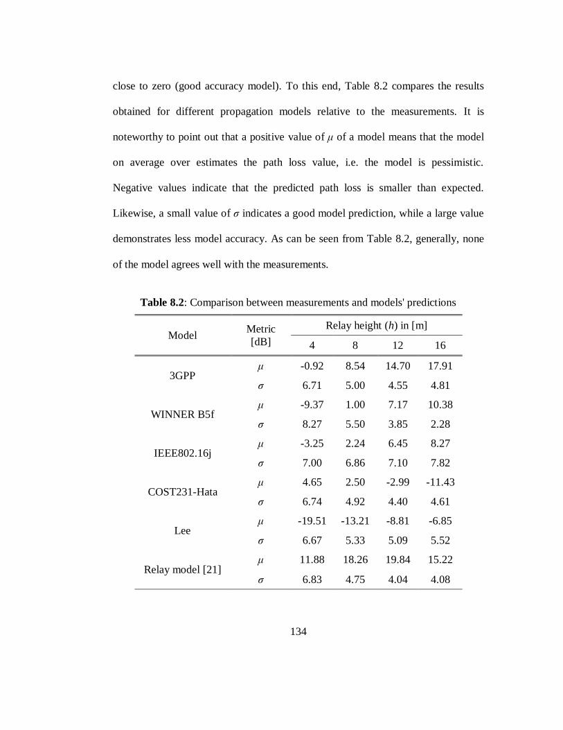
134
close to zero (good accuracy model). To this end, Table 8.2 compares the results
obtained for different propagation models relative to the measurements. It is
noteworthy to point out that a positive value of μ of a model means that the model
on average over estimates the path loss value, i.e. the model is pessimistic.
Negative values indicate that the predicted path loss is smaller than expected.
Likewise, a small value of σ indicates a good model prediction, while a large value
demonstrates less model accuracy. As can be seen from Table 8.2, generally, none
of the model agrees well with the measurements.
Table 8.2: Comparison between measurements and models' predictions
Model Metric
[dB]
Relay height (h) in [m]
4 8 12 16
3GPP μ -0.92 8.54 14.70 17.91
σ 6.71 5.00 4.55 4.81
WINNER B5f μ -9.37 1.00 7.17 10.38
σ 8.27 5.50 3.85 2.28
IEEE802.16j μ -3.25 2.24 6.45 8.27
σ 7.00 6.86 7.10 7.82
COST231-Hata μ 4.65 2.50 -2.99 -11.43
σ 6.74 4.92 4.40 4.61
Lee μ -19.51 -13.21 -8.81 -6.85
σ 6.67 5.33 5.09 5.52
Relay model [21] μ 11.88 18.26 19.84 15.22
σ 6.83 4.75 4.04 4.08

135
8.1.4 Individual Evaluation of Existing Models
In the following, performance of each individual propagation model is
compared to the measurements and considered separately. As Table 8.2 shows,
while for h = 8, 12 and 16 3GPP model significantly over predicts the path loss
values, the model matches the measurements with small μ of 0.92 dB for h=4. This
result may be explained by the fact that 3GPP model was developed under
assumptions similar to the h=4 case presented in this work. The 3GPP model was
developed for frequency of 2GHz, base station antenna height of 30 m and relay
height of 5 m. On the other hand, the lack of relay antenna height correction factor
of 3GPP model for heights different than 4 m leads to the mismatch between model
predictions and measurements in the cases of h =8, 12 and 16 m. The model
accuracy ranges from 4.81 to 6.71 dB. As a final comment, in the case of h=4 m,
results show that 3GPP model is the best candidate among other models.
Consider now WINNER B5f model. Even though it gives the lowest
prediction error (µ=1 dB) in the case of h=8 m, the model badly predicts the path
loss when compared with measured data for all relay heights. Having a small µ
does not necessarily mean that the model prediction matches the measurements
because the error is averaged over the entire measurements. Therefore, the error
statistics are not an appropriate evaluation metric in such cases. To evaluate the
model prediction under similar circumstances, one should consider graphical
performance illustration instead (see Figure 8.2). This figure clearly shows the

136
mismatch between the measurements and the model prediction. This is due to the
fact that WINNER B5f model has relatively small slope value compared to the
measurements and other models. Nevertheless, it is apparent form Figure 8.4 (h=16
m) that if model predictions had been shifted down by some value, they would have
followed the measurements. According to Table 8.2, this shift is 10.38 dB which is
the mean of the prediction error. Except for this shift, there is an agreement
between the model predictions and the measurements with very small standard
deviation of 2.28 dB. This result could be attributed to the fact that there is a
similarity in the assumptions between measurements and WINNER B5f model. It
seems possible that the model over estimates the actual path loss values by 10.38
dB, on average, because WINNER B5f model was designed for urban relaying
cellular scenarios and not for suburban ones where the measurements were carried
out. Similar to 3GPP model, WINNER B5f model was developed for a certain level
of relay height and does not provide an antenna height correction factor. For this
reason model predictions remain the same for all relay height levels. Therefore,
path loss predictions made by WINNER B5f are not reliable especially for relay
heights lower than 16 m. Such discrepancy with measured data is also highlighted
in previous studies and reported in [21].
Concerning now IEEE802.16j model. Unlike the 3GGP and WINNER B5f
models, this model has a correction factor for the relay antenna height.
Nevertheless, the model predictions are incoherent with the measurements. This
137
incoherence is pronounced and can be easily seen for the higher levels of relay
heights (see Figure 8.3 and Figure 8.4). Quantitatively, this is also clear since both
µ and σ are relatively large and more than 6 dB and 7 dB, respectively for relay
heights greater than 10 m. This is because the model is not valid for relay heights
greater than 10 m. For relay heights 4 and 8 m, the model underestimates the actual
path loss especially for distances closer to the transmitter (Figure 8.1 and Figure
8.2). It is clear from the previous figures that the model exhibits quit large slope
(m=45 dB/decade) compared to the measurements. It is somewhat surprising that
even for relay heights lower than 10 m for which antenna height correction factor
was provided, the model predictions do not match the measurements. This was
unexpected because the model was proposed for relaying scenarios. This
conclusion of mismatch between IEEE802.16j model predictions and
measurements supports the finding in the previous study [21] which ended up with
the same conclusion.
Even though COST231-Hata model provides receive antenna height
correction factor, its prediction, in general, is not in a good agreement with the
measurements. While the model over predicts the path loss for lower relay heights,
its underestimation is noticeable for higher relay heights. However, the model
predictions for medium relay heights, namely h=8 m and h=12 m, are much better.
The average prediction error is between 2.5 and 3 dB for medium relay heights and
the model accuracy ranges from 4 to 5 dB. For the case when h=16 m, the average
138
error exceeds 11 dB. A possible explanation for this might be that the associated
antenna height correction factor for the COST231-Hata model is not valid for
heights beyond 10 m. In general, the mismatch with the measurements for all relay
heights is due the fact that COST231-Hata model does not take the clutter and
terrain profile into account. In addition, the model is an extension version of Hata
model which was developed in Japanese and European cities. In general, these
cities tend to have different clutter and terrain profile than US cities. Another
possible explanation for the observations is that COST231-Hata model is most
appropriate for mobile scenarios rather than relaying deployment where typical
antenna heights are between 4 and 16 m.
Turning now to Lee model. The model seems to be very optimistic in
predicting path loss. The average prediction error exceeds 19 dB for the lowest
relay height and it is about 7 dB for the highest one as it shown in Table 8.2. Even
though the model gives very large error for the case when h=4 m, the slope of the
model (m=38.4 dB/dec.) is very close to the one obtained from the measurements
(m=38.54 dB/dec.) as it can be seen from Figure 8.1. In other words, if Lee model
curve had been shifted up by the average error value (µ=19.51 dB), it would have
matched the measurements. Except for this shift, there is an agreement between the
model predictions and the measurements with a standard deviation (σ) of 6.67 dB.
Note that this value of σ is exactly the same one obtained from the measurements.
139
This indicates that the accuracy of the model proposed for h=4 m in this study is
similar to Lee model's accuracy.
Finally, the relay model proposed in [21] which was designed for relay link
over predicts the actual path loss at all relay heights. The prediction error ranges
from 15 dB to about 20 dB. The standard deviation of the error is between 4 dB and
7 dB. The mismatch with the measurements is due to the constraints that are
associated with the relay model. Among the constraints is the difference in the
environment in which both measurement campaigns were conducted. While the
measurements in the presented research were performed in suburban environment,
the relay model was designed for relaying deployment in urban one. Additionally,
the model is valid for distances that are much shorter compared to the ones
proposed in this work, namely 1000 m versus 4000 m. It can be concluded that
since the relay model proposed in [21] was designed for relay link in NLOS
conditions in urban environment, its applicability in different area is not valid.
8.2 Tuning of Existing Models
As it was mentioned in the introduction of this chapter, the considered
existing propagation models might be divided into two groups according to their
applicability in relaying deployment. Those two groups are standard models for
cellular networks and models which were specifically developed for relaying
scenarios. However, the later ones were derived just for certain level of relay

140
antenna height. Validation of the first group to be applicable in relaying
environments and expanding the second one for different relay heights is achieved
by introducing tuning to the original form of those models.
8.2.1 Tuning of Standard Models
Some well-known examples of standard models are COST231-Hata model
and Lee model. In an attempt to make these already coded models applicable in
relaying scenarios, some modifications of their original forms are introduced. The
modifications are based on an attempt to make these models follow the
measurements with small prediction errors and high prediction accuracy for relay
heights ranging from 4 to 16 m.
For COST231-Hata model, the adjusted version of the model is given as:
𝑃𝐿𝐴𝑑𝑗. 𝐶𝑂𝑆𝑇231−𝐻𝑎𝑡𝑎[dB] = 𝐴 + 𝐵 log(𝑑) − ∆ℎ − 12.47 (8.14)
where the model parameters are given as follows.
𝐴 = 46.3 + 33.9 log(𝑓) − 13.82 log (ℎ𝑏) (8.15)
where the frequency f falls within the 1900 MHz band and hb is the
transmitter antenna height in meters.

141
𝐵 = 44.9 − 6.55 log (ℎ𝑏) (8.16)
Δh is the relay antenna height correction factor and it is given by:
∆ℎ = [22.21 log (𝑑
𝑑0) + 7.17] log (
ℎ
4) (8.17)
It should be noted that Δh is derived from the measurements as it was
presented in the previous chapter. Note that the difference between the original
COST231-Hata model and the modified version may be explained as follows. The
term Cm, in the original form of COST231-Hata model given in (8.4), was omitted
since its value is equal to zero for suburban environments. Also the receiver height
correction factor a (hm) was replaced by a new one Δh. Finally, an adjusting factor
of 12.47 dB was added to the modified version of the model.
In the case of Lee model, the modified version is given by:
𝑃𝐿𝐴𝑑𝑗. 𝐿𝑒𝑒 = 𝑃𝐿0 +𝑚log(𝑑
𝑑0) − 𝐻𝑇 − 𝛥ℎ − 28.38 (8.18)
The model parameters are identical to those of the original Lee model given
in (8.5) except for the value of d0. The reference distance (d0) is now equal to 100
meters instead of 1 mile (or 1.609 km). The reference distance is changed since it is
quite common to deploy relays at hundreds of meters from the base station. Δh is

142
defined as in (8.17). Comparing the original form of Lee model and the modified
version, one can see that the receive antenna height correction factor has been
replaced and a new adjusting factor of 28.38 dB has been added.
8.2.2 Tuning of Existing Relaying Models
Existing relaying models are referred to 3GPP, WINNER B5f and
IEEE802.16j models. While the former two models were derived for just one level
of relay height, the applicability for the later one was limited to relay heights not to
be exceeded 10 meters. Expanding of those models to be applicable for multiple
relay heights is proposed in this section. The expansion is accomplished by
introducing the relay antenna height correction factor Δh which was derived in the
previous chapter.
The modified version of 3GPP model is now given as:
𝑃𝐿𝐴𝑑𝑗. 3𝐺𝑃𝑃 = 𝑃𝐿3𝐺𝑃𝑃 − 𝛥ℎ + 0.92 (8.19)
where PL3GPP is the predicted path loss calculated by the original 3GPP
model, Δh is defined as in (8.17), and the adjusting factor 0.92 is the average
prediction error (µ) that was provided in Table 8.2.
In the case of WINNER B5f model, the modified version is given by:

143
𝑃𝐿𝐴𝑑𝑗. 𝑊𝐼𝑁𝑁𝐸𝑅 = 𝑃𝐿𝑊𝐼𝑁𝑁𝐸𝑅 − 𝛥ℎ𝑊 − 10.38 (8.20)
where PLWINNER is the path loss prediction made by the original WINNER
B5f model, ΔhW is relay height correction factor, and the adjusting factor 10.38 is
the average prediction error (µ) that was provided in Table 8.2. Note that ΔhW is
slightly different than Δh for other models, and it is defined as:
∆ℎ𝑊 = [22.21 log (𝑑
𝑑0) + 7.17] log (
ℎ
16) (8.21)
The difference between Δh and ΔhW is that the reference relay antenna height
is 4 m for the former one, see (8.17), while for the later one is 16 m, see (8.21).
It is noteworthy to point out that the modified versions of 3GPP and
WINNER B5f models are developed by just adding the appropriate adjusting and
relay antenna height correction factors to the original forms.
Finally, for IEEE802.16j model, it should be noticed that the applicable range
of the receive antenna height was limited to 10 m. The associated receive antenna
height correction factor for IEEE802.16j model is modified so that the model can
be used to predict the path loss in relay scenarios even when h greater than 10 m.
The modified version of IEEE802.16j model is now given by:

144
𝑃𝐿𝐴𝑑𝑗. 𝐼𝐸𝐸𝐸 = 𝐴 + 10𝛾 log (𝑑
𝑑0) + ∆𝑃𝐿𝑓 − ∆ℎ𝐼𝐸𝐸𝐸 (8.22)
where the modified-model parameters are the same as for the original one
except for A and ΔhIEEE which are defined as follows.
𝐴 = 20 log (4𝜋𝑑0𝜆
) (8.23)
and
∆ℎ𝐼𝐸𝐸𝐸 = ∆ℎ4 + ∆ℎ (8.24)
where Δh is defined as in (8.17) and Δh4, the correction factor when h=4 m is
given as:
∆ℎ4 = [6.5log (𝑑
𝑑0) − 9.3] (8.25)
Unlike other models, the new factor Δh4 was necessary in IEEE802.16j model
because its prediction is incoherent with the measurements. As was mentioned
earlier, the incoherence is attributed to the fact that IEEE802.16j model has large
slope (m=45 dB/decade) compared to the measurements and other models (m= 36-
38 dB/decade). For this reason, Δh4 is added along with Δh to the original form of

145
IEEE802.16j model to adjust its slope and make the model prediction follow the
measurements.
8.3 Performance Analysis of Tuned Models
The introduction of the correction factors to the existing models achieves two
main goals. Firstly, 3GPP, WINNER B5f and IEEE802.16j models are now
applicable for multiple relay heights. Additionally, COS231-Hata and Lee models
are now expanded into relaying propagation scenarios.
Table 8.3 provides the final comparison between the extended versions of the
considered models and the measurements. The comparison is made in terms of the
mean (μ) and the standard deviation (σ) of the prediction error. Table 8.3 clearly
shows that the path loss predictions of all discussed models correspond with the
measurements, on the average. For all models, μ is smaller than 0.94 dB, on the
average. Note that σ represents model's accuracy and it ranges from 2.23 dB for
higher relay heights (~16 m) to 6.74 dB for smaller ones (~4 m). These statistical
data are in a good agreement with the results obtained from the measurements and
presented in the previous chapter. Note that σ is getting smaller as the relay antenna
becomes higher. This is because the path loss variations (shadowing effects)
decrease as the link between the transmitter and the receiver becomes clearer.
Based on Table 8.3, it may be concluded that it is possible to make all
considered models perform adequately in relying scenarios and with approximately
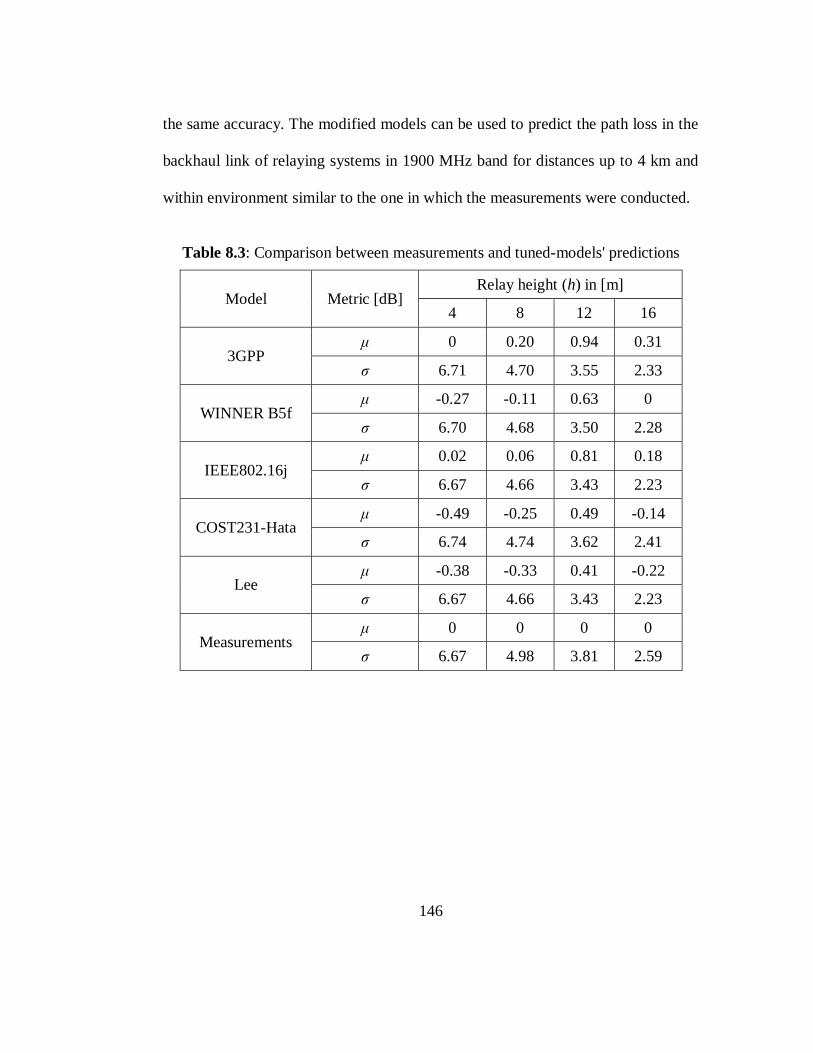
146
the same accuracy. The modified models can be used to predict the path loss in the
backhaul link of relaying systems in 1900 MHz band for distances up to 4 km and
within environment similar to the one in which the measurements were conducted.
Table 8.3: Comparison between measurements and tuned-models' predictions
Model Metric [dB] Relay height (h) in [m]
4 8 12 16
3GPP μ 0 0.20 0.94 0.31
σ 6.71 4.70 3.55 2.33
WINNER B5f μ -0.27 -0.11 0.63 0
σ 6.70 4.68 3.50 2.28
IEEE802.16j μ 0.02 0.06 0.81 0.18
σ 6.67 4.66 3.43 2.23
COST231-Hata μ -0.49 -0.25 0.49 -0.14
σ 6.74 4.74 3.62 2.41
Lee μ -0.38 -0.33 0.41 -0.22
σ 6.67 4.66 3.43 2.23
Measurements μ 0 0 0 0
σ 6.67 4.98 3.81 2.59

147
Chapter 9: Conclusions and Future Work
9.1 Summary and Conclusions
This dissertation presented and analyzed the results of a path loss
measurement campaign conducted in a typical suburban environment. The
campaign was set up specifically to evaluate the path loss in the relay environment.
The measurements are collected in 1900MHz band which is one of the principal
bands for the deployment of the LTE and LTE-Advanced. The study is conducted
using four different relay heights (h) ranging from 4 to 16 m, which are typical
heights where one would find relay deployment in various scenarios. Additionally,
measurements were conducted at street level antenna height (h=1.7 m).
The work presented in this dissertation achieved two major contributions.
Firstly, empirical propagation models for relay environment were proposed and
their statistical analysis were provided. Secondly, a relationship between
measurements and some existing propagation models was established and suitable
correction factors were derived.
Regarding the first contribution, it was found that the path loss may be
modeled successfully with a slightly modified log-distance propagation model. The

148
empirical path loss models for different relay heights presented in this dissertation
were derived from the collected data. The parameters associated with the developed
empirical models include the slope (m) and the intercept (PL0) for each level of the
examined relay heights. The parameters were determined from empirical studies
and through the appropriate linear regression process.
Two different approaches of developing empirical propagation path loss
models for relay environment has been achieved. The first one is with fixed
environmentally dependent slopes and intercepts. In this approach, the relay
antenna height is included in the path loss modeling. Therefore, a general empirical
propagation model which takes into account the effect of relay antenna height was
derived by introducing a distance dependent antenna height correction factor (Δh).
The second approach does not include the relay antenna height correction factor but
the height of the relay antenna becomes part of the slope and intercept calculation.
For both approaches, the analysis results indicate that model predictions are in good
agreement with the measurement.
As far as the second contribution of this work is concerned, it started with the
performance evaluation of some existing propagation models. Five propagation
models namely, 3GPP, WINNER B5f, IEEE802.16j, COST231-Hata and Lee
model have been investigated. The validity of existing propagation models is
examined by comparing their path loss predictions to the measurements. The

149
results of the analysis reveal that the applicability of commonly advocated models
for relaying environment is still questionable. Therefore, appropriate correction
factors were added to their original forms to make all these models perform
adequately. With the proposed correction factors, the analyzed models showed
good agreement with measurements. Furthermore, it is concluded that with proper
correction factors, all the examined models perform adequately and with
approximately the same accuracy.
As a final comment, the proposed empirical models as well as the modified
versions of existing models might be used to predict the path loss at any particular
distance in the backhaul link of relaying systems operating in 1900 MHz band. The
models are valid for any given relay station antenna height between 4 m and 16 m
and within environment similar to one surveyed in the measurement campaign
presented in this dissertation.
9.2 Future Work
The presented work in this dissertation proposed some models that might be used
to predict path loss in relaying environments. Additionally, the measurements were
carried out in a certain environment. As it is known, path loss models perform
differently as the environment changes. Furthermore, the measurements were
conducted in 1900 MHz frequency band only. In practice, however, loss is almost

150
always frequency dependent. Therefore, straightforward extensions of this work
might include the following:
Evaluation of the proposed models performance in different
environments like urban, dense urban or rural areas and consequently
derivation of the appropriate environmentally dependent correction
factors.
Conducting measurements at different frequency bands and
consequently derivation of the appropriate frequency dependent
correction factor.

151
Appendix: Antenna Pattern Data
Horizontal
pattern
Vertical
pattern I
Horizontal
pattern
Vertical
pattern II
Azimuth
angle
Gain
[dB]
Elevation
angle
Gain
[dB]
Azimuth
angle
Gain
[dB]
Elevation
angle
Gain
[dB]
0 6.38 -90 -13.97 180 6.31 -90 -13.97
1 6.37 -89 -12.51 181 6.29 -89 -13.85
2 6.369 -88 -12.62 182 6.281 -88 -13.97
3 6.359 -87 -12.83 183 6.271 -87 -14.48
4 6.349 -86 -12.51 184 6.281 -86 -13.85
5 6.338 -85 -11.92 185 6.282 -85 -14.48
6 6.338 -84 -12.51 186 6.262 -84 -15.15
7 6.328 -83 -12.31 187 6.242 -83 -15.15
8 6.317 -82 -12.51 188 6.233 -82 -16.68
9 6.307 -81 -12.11 189 6.243 -81 -16.19
10 6.297 -80 -12.31 190 6.243 -80 -16.35
11 6.236 -79 -12.51 191 6.164 -79 -16.19
12 6.186 -78 -12.83 192 6.084 -78 -16.04
13 6.136 -77 -12.01 193 6.034 -77 -16.35
14 6.105 -76 -12.31 194 6.005 -76 -16.68
15 6.065 -75 -12.31 195 6.975 -75 -16.19
16 6.045 -74 -12.72 196 6.925 -74 -15.73
17 6.024 -73 -12.62 197 6.866 -73 -15.88
18 6.974 -72 -12.94 198 6.826 -72 -16.19
19 6.884 -71 -13.85 199 6.806 -71 -15.44
20 6.793 -70 -13.5 200 6.777 -70 -15.73
21 6.733 -69 -13.97 201 6.637 -69 -14.88
22 6.663 -68 -13.97 202 6.487 -68 -15.44
23 6.582 -67 -14.1 203 6.378 -67 -14.88

152
24 6.492 -66 -13.73 204 6.308 -66 -15.15
25 6.402 -65 -13.97 205 6.238 -65 -15.01
26 6.331 -64 -14.48 206 6.149 -64 -16.04
27 6.261 -63 -14.88 207 6.059 -63 -16.04
28 6.161 -62 -14.48 208 6.959 -62 -15.58
29 6.02 -61 -14.74 209 6.87 -61 -16.35
30 6.89 -60 -14.22 210 6.78 -60 -16.85
31 6.77 -59 -14.74 211 6.68 -59 -17.38
32 6.649 -58 -14.74 212 6.581 -58 -17.74
33 6.529 -57 -14.88 213 6.491 -57 -18.74
34 6.399 -56 -14.61 214 6.401 -56 -17.94
35 6.268 -55 -14.22 215 6.312 -55 -19.64
36 6.168 -54 -14.74 216 6.192 -54 -22.06
37 6.078 -53 -14.22 217 6.072 -53 -22.06
38 6.957 -52 -14.74 218 6.933 -52 -23.4
39 6.827 -51 -15.29 219 6.803 -51 -23.77
40 6.687 -50 -15.44 220 6.653 -50 -24.56
41 6.586 -49 -15.88 221 6.534 -49 -23.04
42 6.486 -48 -16.85 222 6.404 -48 -21.17
43 6.396 -47 -16.51 223 6.304 -47 -20.37
44 6.325 -46 -18.54 224 6.235 -46 -17.38
45 6.245 -45 -18.74 225 6.175 -45 -15.29
46 6.155 -44 -19.87 226 6.075 -44 -14.35
47 6.074 -43 -20.9 227 6.976 -43 -13.27
48 6.984 -42 -19.64 228 6.876 -42 -12.11
49 6.914 -41 -18.33 229 6.786 -41 -11.18
50 6.833 -40 -17.56 230 6.697 -40 -10.33
51 6.803 -39 -16.35 231 6.677 -39 -9.94
52 6.773 -38 -16.04 232 6.647 -38 -9.06
53 6.722 -37 -15.73 233 6.638 -37 -8.65
54 6.662 -36 -15.58 234 6.638 -36 -8.65
55 6.602 -35 -15.88 235 6.638 -35 -8.59
56 6.651 -34 -15.73 236 6.639 -34 -8.92
57 6.701 -33 -16.04 237 6.639 -33 -9.71
58 6.761 -32 -16.68 238 6.649 -32 -10.58
59 6.82 -31 -15.15 239 6.69 -31 -11.72

153
60 6.88 -30 -13.85 240 6.72 -30 -14.1
61 6.93 -29 -12.21 241 6.78 -29 -16.85
62 6.969 -28 -9.94 242 6.851 -28 -19.4
63 6.029 -27 -8.52 243 6.961 -27 -23.77
64 6.109 -26 -6.92 244 6.111 -26 -19.87
65 6.188 -25 -6.34 245 6.252 -25 -16.85
66 6.298 -24 -5.99 246 6.262 -24 -14.74
67 6.398 -23 -6.04 247 6.272 -23 -13.85
68 6.517 -22 -6.09 248 6.373 -22 -12.94
69 6.627 -21 -6.76 249 6.543 -21 -12.62
70 6.737 -20 -7.83 250 6.713 -20 -13.27
71 6.856 -19 -10.17 251 6.814 -19 -14.74
72 6.976 -18 -12.62 252 6.924 -18 -16.19
73 6.076 -17 -17.02 253 6.014 -17 -19.4
74 6.175 -16 -22.06 254 6.115 -16 -26.39
75 6.275 -15 -17.94 255 6.205 -15 -37.02
76 6.375 -14 -14.74 256 6.315 -14 -23.04
77 6.474 -13 -13.97 257 6.426 -13 -22.37
78 6.594 -12 -14.61 258 6.516 -12 -20.12
79 6.734 -11 -19.64 259 6.596 -11 -20.12
80 6.883 -10 -34.1 260 6.667 -10 -18.13
81 6.933 -9 -14.88 261 6.777 -9 -12.01
82 6.983 -8 -8.08 262 6.887 -8 -7.65
83 6.052 -7 -3.47 263 6.998 -7 -3.92
84 6.122 -6 -0.09 264 6.108 -6 -0.79
85 6.192 -5 2.26 265 6.208 -5 1.73
86 6.221 -4 4.27 266 6.209 -4 3.71
87 6.251 -3 4.64 267 6.209 -3 5.3
88 6.281 -2 5.8 268 6.249 -2 5.63
89 6.32 -1 5.92 269 6.32 -1 5.99
90 6.35 0 6.38 270 6.4 0 6.31
91 6.39 1 6.79 271 6.35 1 6.28
92 6.419 2 6.93 272 6.311 2 6
93 6.449 3 6.82 273 6.301 3 5.99
94 6.449 4 6.46 274 6.311 4 5.65
95 6.448 5 5.82 275 6.332 5 5.17

154
96 6.428 6 5.91 276 6.322 6 5.33
97 6.408 7 5.8 277 6.302 7 5.25
98 6.367 8 4.24 278 6.283 8 4.83
99 6.317 9 2.22 279 6.253 9 3.12
100 6.267 10 -0.34 280 6.223 10 0.71
101 6.206 11 -3.51 281 6.184 11 -2.15
102 6.156 12 -7.71 282 6.134 12 -6.04
103 6.096 13 -15.29 283 6.074 13 -11.63
104 6.045 14 -32.94 284 6.985 14 -24.56
105 6.995 15 -16.85 285 6.895 15 -23.04
106 6.905 16 -14.74 286 6.835 16 -15.29
107 6.824 17 -13.5 287 6.776 17 -13.38
108 6.734 18 -14.98 288 6.696 18 -13.62
109 6.654 19 -17.74 289 6.586 19 -14.35
110 6.573 20 -24.56 290 6.487 20 -20.63
111 6.503 21 -24.56 291 6.377 21 -28.72
112 6.443 22 -16.35 292 6.277 22 -18.33
113 6.332 23 -12.01 293 6.178 23 -12.11
114 6.182 24 -9.27 294 6.088 24 -8.86
115 6.022 25 -7.71 295 6.998 25 -6.81
116 6.921 26 -6.65 296 6.859 26 -5.52
117 6.811 27 -6.24 297 6.729 27 -4.56
118 6.701 28 -6.24 298 6.599 28 -4.03
119 6.57 29 -6.86 299 6.48 29 -3.8
120 6.45 30 -7.54 300 6.36 30 -3.96
121 6.38 31 -8.92 301 6.24 31 -4.51
122 6.299 32 -10.58 302 6.111 32 -5.29
123 6.219 33 -12.51 303 6.021 33 -6.44
124 6.129 34 -15.01 304 6.961 34 -8.08
125 6.038 35 -17.56 305 6.912 35 -10.66
126 6.958 36 -17.02 306 6.822 36 -13.5
127 6.888 37 -18.54 307 6.742 37 -18.54
128 6.827 38 -18.54 308 6.703 38 -25.89
129 6.787 39 -17.74 309 6.703 39 -31
130 6.757 40 -19.18 310 6.703 40 -23.04
131 6.716 41 -21.17 311 6.734 41 -20.12

155
132 6.686 42 -23.04 312 6.764 42 -18.13
133 6.686 43 -28.08 313 6.744 43 -17.02
134 6.715 44 -25.42 314 6.685 44 -16.04
135 6.755 45 -21.17 315 6.63 45 -15.44
136 6.785 46 -18.54 316 6.715 46 -14.1
137 6.824 47 -16.51 317 6.806 47 -13.27
138 6.894 48 -14.48 318 6.886 48 -13.5
139 6.984 49 -13.05 319 6.956 49 -11.92
140 6.083 50 -12.31 320 6.027 50 -11.82
141 6.203 51 -11.72 321 6.127 51 -11.72
142 6.323 52 -11.09 322 6.217 52 -11.26
143 6.422 53 -11.18 323 6.328 53 -11.09
144 6.492 54 -11.45 324 6.428 54 -11.45
145 6.562 55 -11.35 325 6.538 55 -11.63
146 6.701 56 -11.72 326 6.639 56 -12.41
147 6.831 57 -11.92 327 6.749 57 -12.32
148 6.951 58 -12.83 328 6.869 58 -13.38
149 6.06 59 -13.38 329 6.99 59 -13.27
150 6.16 60 -14.1 330 6.12 60 -13.62
151 6.31 61 -15.01 331 6.23 61 -13.85
152 6.449 62 -15.73 332 6.341 62 -13.85
153 6.559 63 -16.85 333 6.461 63 -13.5
154 6.649 64 -18.33 334 6.591 64 -13.62
155 6.738 65 -19.4 335 6.712 65 -13.38
156 6.838 66 -20.63 336 6.832 66 -13.73
157 6.938 67 -22.06 337 6.952 67 -13.62
158 6.037 68 -23.77 338 6.073 68 -13.73
159 6.137 69 -25.89 339 6.183 69 -13.27
160 6.237 70 -28.08 340 6.293 70 -13.38
161 6.316 71 -30.17 341 6.374 71 -13.97
162 6.406 72 -28.72 342 6.454 72 -14.48
163 6.486 73 -28.72 343 6.544 73 -14.88
164 6.565 74 -29.42 344 6.645 74 -14.74
165 6.635 75 -27.48 345 6.735 75 -15.88
166 6.705 76 -24.98 346 6.785 76 -16.19
167 6.774 77 -24.56 347 6.836 77 -15.88

156
168 6.844 78 -22.7 348 6.896 78 -16.68
169 6.904 79 -22.37 349 6.946 79 -17.02
170 6.963 80 -23.04 350 6.007 80 -17.38
171 6.043 81 -22.7 351 6.047 81 -16.68
172 6.123 82 -21.75 352 6.097 82 -17.94
173 6.172 83 -21.46 353 6.158 83 -19.18
174 6.192 84 -20.9 354 6.238 84 -18.33
175 6.212 85 -20.63 355 6.308 85 -19.18
176 6.251 86 -19.64 356 6.309 86 -19.87
177 6.281 87 -21.17 357 6.299 87 -18.54
178 6.301 88 -19.64 358 6.319 88 -19.4
179 6.3 89 -20.37 359 6.35 89 -19.4
180 6.31 90 -20.37 360 6.38 90 -20.37

157
References
[1] (2014). Cisco White paper. Cisco Visual Networking Index: Global Mobile
Data Traffic Forecast Update, 2013–2018. Available:
http://www.cisco.com/c/en/us/solutions/collateral/service-provider/visual-
networking-index-vni/white_paper_c11-520862.html
[2] L. Quartey. (2013). Mobile subscriptions to exceed world's population by
2014 - Report. Available: http://www.theafricareport.com/North-
Africa/mobile-subscriptions-to-exceed-worlds-population-by-2014-
report.html
[3] S. Parkvall, et al., "LTE-Advanced - Evolving LTE towards IMT-
Advanced," in Vehicular Technology Conference, 2008. VTC 2008-Fall.
IEEE 68th, 2008, pp. 1-5.
[4] E. Dahlman, et al., 3G Evolution: HSPA and LTE for Mobile Broadband,
2nd ed.: Academic Press, 2008.
[5] 3GPP, "TR 36.913 V11.0.0: LTE; Requirements for further advancements
for Evolved Universal Terrestrial Radio Access (E-UTRA) (LTE-
Advanced)," Nov. 2012.
[6] R. Pabst, et al., "Relay-based deployment concepts for wireless and mobile
broadband radio," Communications Magazine, IEEE, vol. 42, pp. 80-89,
2004.
[7] D. Soldani and S. Dixit, "Wireless relays for broadband access [radio
communications series]," Communications Magazine, IEEE, vol. 46, pp.
58-66, 2008.
[8] 3GPP, "TR 36.814 V9.0.0: Further advancements for E-UTRA physical
layer spects (Release 9)," March 2010.

158
[9] M. Werner, et al., "Cost Assessment and Optimization Methods for Multi-
Node Radio Access Networks," in Vehicular Technology Conference, 2008.
VTC Spring 2008. IEEE, 2008, pp. 2601-2605.
[10] P. Moberg, et al., "Performance and Cost Evaluation of Fixed Relay Nodes
in Future Wide Area Cellular Networks," in Personal, Indoor and Mobile
Radio Communications, 2007. PIMRC 2007. IEEE 18th International
Symposium on, 2007, pp. 1-5.
[11] E. C. Van Der Meulen, "Three-Terminal Communication Channels,"
Advances in Applied Probability, vol. 3, pp. 120-154, 1971.
[12] T. Cover and A. E. Gamal, "Capacity theorems for the relay channel,"
Information Theory, IEEE Transactions on, vol. 25, pp. 572-584, 1979.
[13] Y. Yang, et al., "Relay technologies for WiMax and LTE-advanced mobile
systems," presented at the Communications Magazine, IEEE, 2009.
[14] J. M. P. Kyösti, L. Hentilä, X. Zhao, "WINNER II Channel Models," IST-4-
027756 WINNER II, D1.1.2 V1.0, September 2007.
[15] G. Senarath, et al., "Multi-hop Relay System Evaluation Methodology
(Channel Model and Performance Metric)," IEEE 802.16j-06/013r3, Feb.
2007.
[16] H. Masui, et al., "Difference of path-loss characteristics due to reception
antenna heights in an urban LOS environment," in Antennas and
Propagation Society International Symposium, 1998. IEEE, 1998, pp. 1672-
1675 vol.3.
[17] H. Masui, et al., "Difference of break-point characteristics due to mobile
antenna heights in microwave urban LOS propagation," in Broadband
Communications, 2000. Proceedings. 2000 International Zurich Seminar
on, 2000, pp. 223-228.
[18] C. L. Law and M. T. Wong, "Wideband indoor channel characterisation
using microstrip patch antennas at 1.95 GHz with different antenna height
configurations," Electronics Letters, vol. 32, pp. 793-795, 1996.
[19] A. Ando, et al., "Effects of receiver antenna height and polarization on
received signal levels at road level from transmitter antennas set in
manhole," in Antennas and Propagation (APSURSI), 2011 IEEE
International Symposium on, 2011, pp. 2399-2402.

159
[20] C. Quang Hien, et al., "On the impact of receive antenna height in a LTE-
Advanced relaying scenario," in European Wireless Technology Conference
(EuWIT) 2010, pp. 129-132.
[21] C. Quang Hien, et al., "Propagation path loss models for LTE-advanced
urban relaying systems," in Antennas and Propagation (APSURSI), 2011
IEEE International Symposium on, 2011, pp. 2797-2800.
[22] I. Rodriguez, et al., "Evaluation of Potential Relay Locations in a Urban
Macro-Cell Scenario with Applicability to LTE-A," in Vehicular
Technology Conference (VTC Spring), 2012 IEEE 75th, 2012, pp. 1-5.
[23] W. Zhenyu, et al., "Statistical peer-to-peer channel models for outdoor
urban environments at 2 GHz and 5 GHz," in Vehicular Technology
Conference, 2004. VTC2004-Fall. 2004 IEEE 60th, 2004, pp. 5101-5105
Vol. 7.
[24] M. Webb;, et al., "Mobile Multihop: Measurements vs. Models," European
Cooperation in the Field of Scientific and Technical Research, 2007.
[25] V. S. Abhayawardhana, et al., "Comparison of empirical propagation path
loss models for fixed wireless access systems," in Vehicular Technology
Conference, 2005. VTC 2005-Spring. 2005 IEEE 61st, 2005, pp. 73-77 Vol.
1.
[26] K. G. Tan and T. A. Rahman, "Receiving antenna height dependence of
radio propagation path loss in fixed wireless access environment," in
Microwave Conference, 1999 Asia Pacific, 1999, pp. 797-800 vol.3.
[27] K. G. Tan and T. A. Rahman, "The effect of receiving antenna height on
temporal fading characteristics in fixed-to-fixed radio propagation channel,"
in Microwave Conference, 1999 Asia Pacific, 1999, pp. 801-804 vol.3.
[28] H. Chia Leong, et al., "Wideband tapped delay line channel model at 3.5
GHz for broadband fixed wireless access system as function of subscriber
antenna height in suburban environment," in Information, Communications
and Signal Processing, 2003 and Fourth Pacific Rim Conference on
Multimedia. Proceedings of the 2003 Joint Conference of the Fourth
International Conference on, 2003, pp. 386-390 Vol.1.
[29] J. Zander, "On the cost structure of future wideband wireless access," in
Vehicular Technology Conference, 1997, IEEE 47th, 1997, pp. 1773-1776
vol.3.

160
[30] A. Furuskar, et al., "An infrastructure cost evaluation of single- and multi-
access networks with heterogeneous traffic density," in Vehicular
Technology Conference, 2005. VTC 2005-Spring. 2005 IEEE 61st, 2005,
pp. 3166-3170 Vol. 5.
[31] H. Huining, et al., "Range extension without capacity penalty in cellular
networks with digital fixed relays," in Global Telecommunications
Conference, 2004. GLOBECOM '04. IEEE, 2004, pp. 3053-3057 Vol.5.
[32] Abdallah Bou Saleh, et al., "On the coverage extension and capacity
enhancement of inband relay deployments in LTE-advanced networks,"
Journal of Electrical and Computer Engineering - Special issue on
LTE/LTE-advanced cellular communication networks, vol. 2010, 2010.
[33] S. Khakurel, et al., "Optimal relay placement for coverage extension in
LTE-A cellular systems," in Communications (NCC), 2012 National
Conference on, 2012, pp. 1-5.
[34] E. Dahlman, et al., 4G: LTE/LTE-Advanced for Mobile Broadband, 2nd ed.:
Academic Press, 2014.
[35] T. S. Rappaport, Wireless Communications:Principles and Practice, 2nd ed.
New Jersey: Prentice Hall, 2002.
[36] S. R. Saunders and A. Aragn-Zavala, Antennas and Propagation for
Wireless Communication Systems 2nd ed.: John Wiley and Sons, 2007.
[37] M. F. Iskander and Y. Zhengqing, "Propagation prediction models for
wireless communication systems," Microwave Theory and Techniques,
IEEE Transactions on, vol. 50, pp. 662-673, 2002.
[38] K. Rizk, et al., "Two-dimensional ray-tracing modeling for propagation
prediction in microcellular environments," Vehicular Technology, IEEE
Transactions on, vol. 46, pp. 508-518, 1997.
[39] G. Liang and H. L. Bertoni, "A new approach to 3-D ray tracing for
propagation prediction in cities," Antennas and Propagation, IEEE
Transactions on, vol. 46, pp. 853-863, 1998.
[40] G. Evans, et al., "The optimization and application of the W.C.Y. Lee
propagation model in the 1900 MHz frequency band," in Vehicular
Technology Conference, 1997, IEEE 47th, 1997, pp. 87-91 vol.1.

161
[41] W. C. Y. Lee, Mobile Communications Design Fundamentals, 2nd ed.:
Wiley, 1993.
[42] Y. Okumura, et al., "Field strength and its variability in VHF and UHF land
mobile service," Review Electrical Communication Laboratory, vol. 16, pp.
825–873, Sept.-Oct 1968.
[43] M. Hata, "Empirical formula for propagation loss in land mobile radio
services," IEEE Transactions on Vehicular Technology, vol. VT-29, pp.
317-325, Aug. 1980.
[44] Thomas Kürner, "Propagation Models for Macro-Cells," in Digital mobile
radio towards future generation systems, final report, 1st ed, 1999.
[45] W. Cheng-Xiang, et al., "Cooperative MIMO channel models: A survey,"
Communications Magazine, IEEE, vol. 48, pp. 80-87, 2010.
[46] V. Erceg, et al., "An empirically based path loss model for wireless
channels in suburban environments," IEEE Journal on selected Areas in
Communications, vol. 17, pp. 1205-1211, 1999.
[47] 3GPP, "TR 36.826 V11.0.0: Relay radio transmission and reception
(Release 11)," Sep. 2012.
[48] M. Hmaid and I. Kostanic, "Path loss measurements for relay stations in
1900 MHz band," in Proceedings of The World Congress on Engineering
and Computer Science 2013, WCECS 2013, San Francisco, CA,USA, 2013,
pp. 736-741.
[49] M. Hamid and I. Kostanic, "Path Loss Prediction in Relay Station
Environment," in Transactions on Engineering Technologies, Special Issue
of the World Congress on Engineering and Computer Science 2013, H. K.
Kim, et al., Eds., ed: Springer Netherlands, 2014, pp. 403-416.
[50] M. Hamid and I. Kostanic, "Path Loss Models for LTE and LTE-A Relay
Stations," Universal Journal of Communications and Network, vol. 1(4), pp.
119-126, 2013.


![The Distribution of Path Loss Exponent in 3D Indoor …[6], [7] path loss configuration is needed for estimating path loss signal in an indoor environment, [8]verification area, and](https://static.fdocuments.in/doc/165x107/5e9732c5ae1913068027223d/the-distribution-of-path-loss-exponent-in-3d-indoor-6-7-path-loss-configuration.jpg)