a) herbicide resistance of Wild Oat in RLP b) estimation ...

Aalto University
School of Science
Degree Programme in Computer Science and Engineering
Mudassar Abbas
Statistical Estimation of Wild Animal
Population in Finland:
A Multiple Target Tracking Approach
Master’s Thesis
Espoo, December 9, 2011
Supervisor: Professor Jouko Lampinen
Instructors: Docent Simo Sarkka
Docent Aki Vehtari
Aalto University
School of Science
Degree Programme in Computer Science and Engineering
ABSTRACT OF
MASTER’S THESIS
Author: Mudassar Abbas
Title:
Statistical Estimation of Wild Animal Population in Finland: A Multiple Target
Tracking Approach
Date: December 9, 2011 Pages: 68
Professorship: Computational Engineering Code: S-114
Supervisor: Professor Jouko Lampinen
Instructors: Docent Simo Sarkka
Docent Aki Vehtari
Control and management of wild animals, especially large carnivores, is an im-
portant task for game and wildlife management authorities all over the world.
Central to the scheme of wild animal conservation is the population size esti-
mation methodology which depends on the used data sampling technique. The
index based data sampling method has been found suitable in the case of large
carnivores. On the other hand, telemetry data has been used to learn the indi-
vidual movement of animals. Subsequently, mathematical modeling is utilized in
order to learn both animal population dynamics and animal movement behavior.
In that context, stochastic state-space models have proved to be appropriate for
handling uncertainty that occurs in the process and observation models.
This thesis provides a novel approach for the estimation of wild animal popula-
tion. We utilize the state-space modeling framework as well as animal movement
models on an unconventional observation and index based dataset. We formulate
the problem as a conditionally linear Gaussian state-space model and recursively
estimate the state of the animals. More specifically, we reformulate the prob-
lem as a special case of multiple target tracking, which can be solved by using
Bayesian optimal filtering methodology. The solution to the problem of tracking
an unknown number of targets is exactly applicable to our animal observation
datasets.
Keywords: Bayesian Inference, Sequential Monte Carlo Method, Kalman
Filter, Multiple Target Tracking, Data Association
Language: English

Acknowledgements
I would like to express my sincere gratitude to Dr. Simo Sarkka for his immense
support and guidance throughout the development of this project and thesis. I also
wish to extend my deepest appreciation to Dr. Aki Vehtari for his continuous advice
and encouragement. My sincere appreciation is extended to Prof. Jouko Lampinen
for his support.
I would also like to extend my sincere appreciation to Mr. Samuli Heikkinen and
Mr. Mika Kurkilahti from the Finnish Game and Fisheries Research Institute for
their contributions to the project.
Special thanks to Mr. Ville Vaananen for his insightful feedback on the thesis
and contributions to the project. I also wish to thank M.Sc. Marianne Hanhela
for her contributions to the project. I am also thankful to all the colleagues at
the Biomedical Engineering and Computational Science department for providing
a special working environment. I wish to extend my appreciation to M.Sc. Jouni
Hartikainen for his help and support.
I am immensely grateful to my parents for providing me the opportunities to
follow my dreams. I am also especially grateful to all my friends and family for their
love and support.
Espoo, December 9, 2011
Mudassar Abbas
3
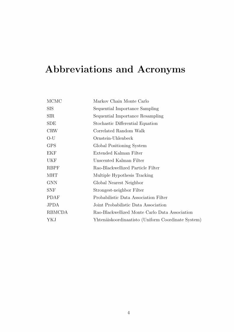
Abbreviations and Acronyms
MCMC Markov Chain Monte Carlo
SIS Sequential Importance Sampling
SIR Sequential Importance Resampling
SDE Stochastic Differential Equation
CRW Correlated Random Walk
O-U Ornstein-Uhlenbeck
GPS Global Positioning System
EKF Extended Kalman Filter
UKF Unscented Kalman Filter
RBPF Rao-Blackwellized Particle Filter
MHT Multiple Hypothesis Tracking
GNN Global Nearest Neighbor
SNF Strongest-neighbor Filter
PDAF Probabilistic Data Association Filter
JPDA Joint Probabilistic Data Association
RBMCDA Rao-Blackwellized Monte Carlo Data Association
YKJ Yhtenaiskoordinaatisto (Uniform Coordinate System)
4
Contents
Abbreviations and Acronyms 4
1 Introduction 9
1.1 Overview of Problem . . . . . . . . . . . . . . . . . . . . . . . . . . . 11
1.2 Structure of Thesis . . . . . . . . . . . . . . . . . . . . . . . . . . . . 12
2 Background 13
2.1 Finnish Politics and Animal Conservation . . . . . . . . . . . . . . . 13
2.2 Animal Abundance . . . . . . . . . . . . . . . . . . . . . . . . . . . . 15
2.2.1 Estimation Methods . . . . . . . . . . . . . . . . . . . . . . . 15
2.2.2 Population Dynamics Modeling . . . . . . . . . . . . . . . . . 17
2.2.3 State-space Models of Animal Population . . . . . . . . . . . . 20
2.2.4 State-space Models of Animal Movement . . . . . . . . . . . . 21
2.3 Bayesian Optimal Filtering . . . . . . . . . . . . . . . . . . . . . . . . 23
2.3.1 Kalman Filter . . . . . . . . . . . . . . . . . . . . . . . . . . . 24
2.3.2 Particle Filtering . . . . . . . . . . . . . . . . . . . . . . . . . 25
2.3.3 Rao-Blackwellized Particle Filtering . . . . . . . . . . . . . . . 27
2.4 Target Tracking and Data Association . . . . . . . . . . . . . . . . . 29
3 Materials, Models and Methods 33
3.1 Data Sources . . . . . . . . . . . . . . . . . . . . . . . . . . . . . . . 33
3.2 Data Format . . . . . . . . . . . . . . . . . . . . . . . . . . . . . . . 37
3.3 Model . . . . . . . . . . . . . . . . . . . . . . . . . . . . . . . . . . . 40
3.4 Method . . . . . . . . . . . . . . . . . . . . . . . . . . . . . . . . . . 41
4 Results 46
5 Conclusion and Discussion 62
5

List of Tables
3.1 Data Attributes . . . . . . . . . . . . . . . . . . . . . . . . . . . . . . 38
3.2 Bear Observations . . . . . . . . . . . . . . . . . . . . . . . . . . . . . 39
3.3 Wolf Observations . . . . . . . . . . . . . . . . . . . . . . . . . . . . . 39
3.4 Lynx Observations . . . . . . . . . . . . . . . . . . . . . . . . . . . . 39
3.5 Wolverine Observations . . . . . . . . . . . . . . . . . . . . . . . . . . 39
4.1 Bear foot widths for different seasons . . . . . . . . . . . . . . . . . . 46
6
List of Figures
2.1 Single target tracking with a single sensor . . . . . . . . . . . . . . . 29
2.2 Single target tracking with multiple sensors . . . . . . . . . . . . . . . 30
2.3 Multiple target tracking with multiple sensors . . . . . . . . . . . . . 30
3.1 Brown bear and foot sizes . . . . . . . . . . . . . . . . . . . . . . . . 34
3.2 Wolf and foot size . . . . . . . . . . . . . . . . . . . . . . . . . . . . . 35
3.3 Lynx and foot size . . . . . . . . . . . . . . . . . . . . . . . . . . . . 36
3.4 Wolverine and foot size . . . . . . . . . . . . . . . . . . . . . . . . . . 37
4.1 Bear observations in Finland for the year 2010. A single observation
can consist of a single individual or a family of bears. In this dataset,
a large number of observations consist of at least a single adult and
a single cub information. . . . . . . . . . . . . . . . . . . . . . . . . . 51
4.2 (a) Different estimated number of targets in time, (b) Best estimate
of the total number of targets, (c) True Group distribution, (d) Group
distribution for the best estimate of the total number of targets. . . . 53
4.3 The results of the RBMCDA are visualized over the map of Finland.
The square box represents a single location close to the southeastern
border of Finland. The integer values are group numbers where each
group can consist of a single observation or multiple observations. . . 54
4.4 Left column: true bear observation groups in three different locations.
Right column: corresponding data association results . . . . . . . . . 55
4.5 (a) Different estimated number of targets in time, (b) Best estimate
of the total number of targets, (c) True Group distribution, (d) Group
distribution for the best estimate of the total number of targets. . . . 56
4.6 Left column: true bear observation groups in three different locations.
Right column: corresponding data association results . . . . . . . . . 57
4.7 Estimated group distribution of bear observations (2009) . . . . . . . 58
7

LIST OF FIGURES 8
4.8 Large carnivore observations in Finland for the year 2009. A sin-
gle observation can consist of a single individual or a family/pack of
animals. . . . . . . . . . . . . . . . . . . . . . . . . . . . . . . . . . . 59
4.9 Estimated group distribution of wolf observations (2009) . . . . . . . 60
4.10 Estimated group distribution of lynx observations (2009) . . . . . . . 60
4.11 Estimated group distribution of wolverine observations (2009) . . . . 61
Chapter 1
Introduction
For more than half a century now it has been appreciated that wild animals enact
an essential role in maintaining the biological diversity of the ecosystem. Therefore,
considerable effort has been taking place all over the world for the conservation of
wild animals especially in the case where some species face extinction. However,
at times a species can be given the ’pest’ status when it exceeds a certain limit of
abundance and it can cause considerable damage to human life and property (De-
lahay and Wilson, 2001). Then a reasonable balance would have to be insured with
appropriate control programs. These are the fundamental reasons for the control
and management of wild animal populations. Central to the scheme of wild animal
population monitoring and management is the estimation of the population size. A
large number of methods have been developed and deployed by biologists, ecologists
and wildlife managers to attain this goal (Southwood and Henderson, 2000; Schwarz
and Seber, 1999).
Methods used in estimating the size of wild animal population can be classified
to two main groups: true abundance methods and index based methods (Delahay
and Wilson, 2001). True abundance can further produce two types of count: a
complete count (census) and an incomplete count (survey). A complete count can
be obtained when the assumption that all the animals would be counted is true while
an incomplete count only samples from a proportion of the total animal population.
Surveys can be conducted by using vehicles, airplanes and imagery technologies.
A more favored statistical approach of surveying is the capture-recapture method
which is mainly used in fisheries. This approach implies that the species is in some
way caught and marked by the field researchers. The methods of marking include
tagging, banding and painting. This method of sample collection is also known as
mark-recapture in animal ecology.
9
CHAPTER 1. INTRODUCTION 10
On the other hand an index based methodology requires that the field personnel
avoid direct interaction with the animal. In this case observation of field-signs
(remains) of the animals is a crucial methodology, for example, observation of habitat
structure and carcasses of dead prey, identifying tracks (foot-prints) and marks
left on plants, and finding feces and animal hair. More recent advances in index
based techniques consist of methods like DNA analysis of hair, feather, feces, dung,
saliva and shed skin (Mills et al., 2000). Moreover, DNA analysis can also be
used in capture-recapture where the sample is taken directly from the body of the
animal (Madon et al., 2011). However, capture-recapture methods involve significant
human effort and expenditure especially in the case of large carnivores because of
their secretive and nocturnal nature. At the same time predicting the exact home
range of large carnivores is very difficult. Therefore, incomplete counts and index
based approaches appear more practical and often preferred especially by wild life
managers for monitoring of large areas (Witmer, 2005; Pollock et al., 2002).
More often, surveys can be conducted sequentially year after year to learn the
dynamics of animal population. Consequently, prediction and management decisions
have to be based on dynamic population models. These models can be formulated as
population-growth models which consist of parameters indicating population-growth
rate. A population can grow because of birth and immigration but simultaneously
reduce due to death and emigration. Similarly, dynamic population models can be
based on an age-structure formulation. The age-structure based models divide the
total animals surveyed into age groups. In these models parameters like survival
and reproduction rate replace the birth and death count parameters. Furthermore,
population models can be density dependent or density independent with the former
being more complex kind of models.
Realistic population dynamics models must incorporate the stochasticity inher-
ent in the actual underlying processes. Process variation and the variation due
to sampling necessitates statistical approaches that incorporate these uncertainties
into the models. Therefore, a statistical modeling approach known as state-space
modeling has been widely acknowledged as a flexible and appropriate approach to
population dynamics models (Buckland et al., 2004b, 2007). Although population
dynamic models can include animal movement (immigration, emigration) in the form
of probability distributions (probability of moving from one location to the other),
more dense positional data available with the advancement in radio telemetry and
GPS telemetry has allowed scientists to study animal movement and habitat behav-
ior on an individual scale (Borger et al., 2008). The classical models of individual
CHAPTER 1. INTRODUCTION 11
animal movement comprises of stochastic differential equations (SDE) (Brillinger
et al., 2002; Preisler et al., 2004). Since observational data from telemetric devices
is also prone to error (noise), use of statistical approaches, specifically state-space
modeling, has been favored in order to link the dynamic models of animal movement
to the observational data (Patterson et al., 2008).
Modeling of individual animal movement based on telemetry data has increased
the knowledge about many social and habitual behaviors of species. However, it
has been less beneficial for the management and conservation of animals on a large
scale (Morales et al., 2010). This is mainly due to the high expenses of acquiring
telemetry data and low feasibility of tagging a large number of animals. Therefore,
methods of estimating animal populations based on surveys and index data have
to be developed and improved with a focus on utilizing the current computational
power of modern computers. In this thesis, we propose a novel approach based on
an unconventional observation and index based survey data. We utilize both state-
space modeling framework and animal movement models in order to estimate the
animal population.
1.1 Overview of Problem
We focus on the analysis of sampling data, which is based on both field-signs and
direct sightings of the animals. A single record in the dataset can consist of informa-
tion about a single individual or group of animals (family or pack). The information
can be either from direct sightings or field-signs of the animals. Field signs consist
of foot print measurements, feces observation, carcass of dead animal or prey and
in some cases habitat structure or animal marks. The data collection process is
based on observations obtained on a regular basis throughout the year from almost
every part of Finland. The accumulated datasets consist of a far greater number of
observations than the actual number of animals. On the contrary, in the index-data
based population estimation methods, the population survey is usually conducted in
smaller regions and shorter time frames and the result of estimation is extrapolated
to larger regions.
The data collection method in our case is unconventional and the standard
methodology of animal abundance estimation becomes inapplicable. The present
method used to estimate population size from this data requires a significant amount
of manual work which involves sorting the information and finding duplicate obser-
vations of the same individual or group of animals that have been observed by

CHAPTER 1. INTRODUCTION 12
multiple observers. Therefore, we propose a state of the art technique which solves
the current problem of population estimation from the unusual data source com-
putationally, without the need for manual work. We formulate the problem as a
conditionally linear Gaussian state-space model and recursively estimate the state
of the animals. More specifically, from the engineering perspective this strategy is
known as optimal filtering.
The problem of estimating the state of multiple targets from noisy measure-
ments generated by multiple sources is referred to as multiple target tracking and
data association problem. This is an application area of optimal filtering. Further-
more, the methodology of data association for an unknown number of targets is ex-
actly applicable to our animal observation datasets. In this thesis, we demonstrate
the applicability of Rao-Blackwellized Monte Carlo data association (RBMCDA)
(Sarkka et al., 2007) algorithm which solves the problem of multiple target tracking
and data association in the case of ‘an unknown number of targets’.
1.2 Structure of Thesis
The organization of this thesis is as follows: the general methods of estimating pop-
ulation size and the background of multiple target tracking methodology is covered
with detail in Chapter 2, Chapter 3 presents the materials, methods and models uti-
lized in the thesis, Chapter 4 shows the results of the study, and Chapter 5 presents
the conclusion and discussions.

Chapter 2
Background
2.1 Finnish Politics and Animal Conservation
Concern has prevailed regarding the extinction of some very rare wild animals among
naturalists, scientists, politicians and common people of Finland for the past fifty
years. Nature reserves and wilderness areas of Finland have been home to four large
carnivores; brown bear (Ursus arctos), wolf (Canis lupus), wolverine (Gulo gulo)
and lynx (Lynx lynx). Since the beginning of the twentieth century the populations
of all four of these fascinating animals has been in decline.
Brown Bear (Ursus arctos)
The brown bear is the national animal of Finland. The estimate of bear population
before the hunting season in 2009 was 1850 to 1950 and at the end of 2009 was 1150
to 1200 (Wikman, 2010). The population density is higher in eastern Finland close
to the Russian border. The brown bear was nearly extinct in Finland around the
beginning of the twentieth century but population has steadily increased since 1970
(Katajisto, 2006), mainly due to migration of bears from Russia.
Wolf (Canis lupus)
Wolf is the most controversial large carnivore in Finland since it causes the highest
threat to livestock, reindeer husbandry and humans. It is for this reason that it has
the smallest population size among the large carnivores of Finland. The estimate of
wolf population in Finland at the end of 2009 was 150 to 160 (Wikman, 2010). The
population density is higher in the eastern regions. Wolves became extinct in the
early twentieth century due to major hunting expeditions. Wolves have also been
13

CHAPTER 2. BACKGROUND 14
subject to severe illegal poaching activities.
Lynx (Lynx lynx)
Lynx has the highest population among the large carnivores of Finland with about
2200 to 2300 individuals reported at the end of 2009 (Wikman, 2010). People have
a more benign attitude towards the lynx or wild cat although it is a very active
predator (Liukkonen et al., 2009). Lynx has an even population density throughout
Finland and the numbers have been increasing since it was protected.
Wolverine (Gulo gulo)
Wolverine is the most elusive animal among the large carnivores of Finland due to
its less dense population structure and large dispersal ability. Population statistics
claim that about 150 to 170 individuals were present at the end of 2009 (Wikman,
2010). It is also one of the most hunted and endangered animal populations of
Finland. The wolverine was nearly extinct until it was protected in 1982.
Organization
The Ministry of Agriculture and Forestry is responsible for the population con-
servation of wild animals in Finland. Legislation concerning hunting licenses and
management plans are approved by the ministry while these plans are based on
research conducted by the Finnish Game and Fisheries Research Institute in par-
ticular. Other organizations which aid the research include, The Hunters Central
Organization which provides sighting data and the Game Management district au-
thorities. The Game Management district authorities license the hunting of animals
under the supervision of the Ministry of Agriculture and Forestry based on the pop-
ulation statistics provided by the Finnish Game and Fisheries Research Institute.
The debate over large carnivore population management largely exists because of
the threat posed by large carnivores to livestock and reindeer husbandry. While the
wild life conservation legislations impose strict laws over the hunting of endangered
species, the farmers and herders have valid reasons for employing safety measures
against the threat caused by wild animals to their property and livestock. However,
the large carnivore population in Finland has suffered not merely because of hunting
and poaching but also due to other environmental and ecological changes in the
natural habitat of the animals.
CHAPTER 2. BACKGROUND 15
2.2 Animal Abundance
Methods for estimating animal abundance (How many are there?) depend on many
factors: landscape of the area where the study or monitoring is taking place, type
of specie which is being studied or monitored and the resources available to con-
duct the study or monitoring. Therefore, careful design of the estimation methods
and procedures is of fundamental importance before initiating the actual field and
analysis work (Witmer, 2005; Pollock et al., 2002).
2.2.1 Estimation Methods
Below, we briefly explain some of the well-known and standard approaches used in
estimating animal abundance. These approaches apply to data obtained through
specific sampling methods or surveys conducted in smaller regions in a fixed time
frame. The individual count obtained through these surveys is often used to estimate
the population density for a small region and the density is extrapolated for larger
areas. However, we need to analyze our data in a more unconventional way because
it is based on unrestricted random observations obtained from a very large area and
over a longer time frame. Further details about the collection of data can be found
in Chapter 3.
Strip and Quadrat Plots
This is a simple method based on counting the animals or field-signs, for example,
feces or foot-prints, over a random set of plots known as sample units. Basically,
the whole region or area, where the animal population estimation has to be accom-
plished, is divided in to smaller regions which can be square or rectangular in shape.
The method of selecting the regions for sampling can vary, more specifications on
sampling procedures can be found in (Anderson, 2001; Thompson et al., 1998). If
random sampling is used and the animals can be directly observed then the method
of estimation consists of the following steps:
• Dividing the whole region into a total of S number of sample units and choosing
s number of sample units randomly where the census would be conducted.
• Counting the total number of animals n in each of the randomly chosen sample
units s:
n =1
s
s∑i=1
ni . (2.1)
CHAPTER 2. BACKGROUND 16
• The abundance estimate can be obtained by multiplying total sampling units
S with n as
n = S n . (2.2)
The abundance estimator can also be divided by the total area of the sampling units
to calculate the population density estimate. Furthermore, a population indices
estimate can also be obtained in case of observation of the field-signs. A single
index must be a constant ratio for the whole population, that is, if the count of
indices doubles then it can be proposed that the whole population has doubled
(Schwarz and Seber, 1999).
Distance Sampling
This method mainly consists of two types; line transects and point counts. Line
transects usually involves an observer moving by foot or in a vehicle along a random
path and sighting the animals. The abundance is then calculated as number of
animals sighted divided by the detection probability which is based on the distance
between the observer and the animal. The detection probability also depends on
the terrain detail, for example, it is higher for plain regions and lower for hilly areas.
If an aerial survey is conducted using this method then the detection probability
is not merely dependent on the distance between the animal and the observer but
many other factors would be involved as well (Buckland et al., 2004a).
Capture-recapture
This method involves marking or tagging of animals during the initial sampling
and then releasing them for the second sampling phase. The next sampling phase
consists of marked and unmarked animals and estimation based on this data includes
different methods and assumptions (Pollock, 2000; Buckland et al., 2000). One of
the more well known methods to estimate the abundance with capture-recapture
data is the Lincoln-Petersen model (Seber, 1986). This method comprises of a few
assumptions; 1- only single recapture event, 2- closed population (excluding births,
deaths or movement outside the region of study), 3- both recapture events have
equal capture probabilities and 4- the marks or tags remain intact. If n1 is the
number of individuals captured and marked during the initial sampling, n2 is the
number of unmarked individuals during the second sampling and m2 the number of
recaptured individuals then the estimator is given by
n =n1 n2
m2
. (2.3)
CHAPTER 2. BACKGROUND 17
Removal Methods
Removal methods include two well-known models; the catch-effort model and the
change-in-ratio model. Catch-effort models have primarily been used in fisheries
with the assumptions that the population is closed and the probability of each indi-
vidual being caught is equal. The catch per effort decreases with more individuals
being caught (removed from the population) because there would be less individu-
als remaining to be caught. Change-in-ratio methods require the population to be
closed and the population to be divided in to two groups, for example, male and
female, adult and infant or two different species. The idea is to remove more individ-
uals from one of the groups and observe the change-in-ratio during the resampling
phase. Estimating the change-in-ratio before and after the sampling reveals other
population parameters as well (Seber, 1986).
Index Scores
This method is used when only the field-signs of the animals can be observed. The
assumption is that the frequency of observations is related to the actual number
of animals. This method provides a relative estimate of abundance or “Index” of
population density (Schwarz and Seber, 1999). Estimate of animal abundance can
be deduced from “index scores” if they can be adjusted with estimates from another
formal estimation method used in parallel (Delahay and Wilson, 2001).
2.2.2 Population Dynamics Modeling
Next, we shall briefly discuss some of the well-known population dynamics mod-
els. These models require sampling of specific parameters during the surveys, for
example, birth date/time, death, movement in and out of sampling region and age-
structure of the population. This information is obtained usually by capturing and
tagging animals. However, this information is unavailable in our data because it is
sighting and index based which restricts the use of these models. Nevertheless, the
estimation method we have used can incorporate population dynamics models as
well.
Detecting each animal with the same certainty is hardly possible, observations
can be biased due to insufficient field related experience of the observer, tags and
marks can be misplaced or lost, and most importantly surveys on a large geographi-
cal area and a longer time scale must be able to address an open population (births,
deaths and movement) (Schwarz and Seber, 1999; Durban and Elston, 2005). Math-
CHAPTER 2. BACKGROUND 18
ematical models can incorporate the dynamics of an open population. This is called
population dynamics modeling and the goal is to predict the future estimate of
animal abundance which aids the decision making process.
Population Growth Models
Population growth model is usually concerned with four important parameters:
birth, death, immigration and emigration (White, 2000). A population-growth
model which is independent of the population density can be represented by a simple
difference equation of the form
nt+1 = nt (1 + r), (2.4)
where nt can be the number of animals in a day,month or year and
r =(birth− death) + (immigration− emigration)
time.
Thus, population growth rate can be given by
λ =nt+1
nt= 1 + r . (2.5)
In case that the time scale unit is years then the Equation (2.5) gives the annual
growth rate and λ < 1 would indicate a decreasing population. Furthermore, the
model in Equation (2.4) can be made more realistic by making it density dependent
because it exhibits exponential population growth. Furthermore, animal populations
depend on the resources (food, water) available in their shared habitat and only a
sufficient amount of resources promise a steady growth in the population size. This
implies that the population growth is a function of the population size
r(nt) = r0(1−ntk
), (2.6)
where k is known as the carrying capacity and r0 is the maximum growth rate for
an extremely small population size. The carrying capacity is a property of the envi-
ronment; it is the maximum limit in terms of population size that an environment
can support without constant degradation of the resources. Substituting expression
in Equation (2.6) to the model Equation (2.4) gives
nt+1 = nt[1 + r0(1−ntk
)] . (2.7)
The models in Equation (2.4) and Equation (2.7) can also be represented with
differential equations for the continuous time case but animal populations exhibit
discrete birth pulses. Therefore, we restrict our discussion to only discrete time
cases.
CHAPTER 2. BACKGROUND 19
Age Based Models
Another form of population models known as age-structured models tend to be
more complex but at the same time they can be more realistic. In age-structured
population models the parameters of birth and death can be replaced by survival
(mortality) and reproduction (fertility) parameters. Again age-structured popula-
tion models can be formulated both as density independent age-structure models
or density dependent age-structure models with the lateral being more realistic and
more complex. A famous formulation of age-structured models in the form of ma-
trices was given by (Leslie, 1945). The Leslie Matrix population model is used to
determine the growth of a population, as well as the age distribution with in the
population over time. The Leslie Matrix population model is given as
nt+1 = Ant, (2.8)
where nt is a vector with components representing the number of individuals in each
age group at time t and A is the Leslie matrix. The model in matrix formulation is
given as
n1
n2
n3
...
na−1
t+1
=
b1 b2 b3 . . . ba−1 ba
s1 0 0 . . . 0 0
0 s2 0 . . . 0 0
0 0 s3 ....
......
... .. . . .
...
0 0 0 . . . sa−1 0
n1
n2
n3
...
na−1
t
, (2.9)
where bi : i = 1, 2, . . . , a is the fertility(number of offspring) of a female of age i,
si : i = 1, 2, . . . , a− 1 is the survival probability that an individual of age i at time
t will survive to time t+ 1 and a is the maximum age limit of the particular animal.
Process Variation
Animal population dynamics models need to be stochastic rather deterministic be-
cause animal population growth and reduction involves uncertainty due to latent
natural processes. This phenomenon is termed as process variation (Thompson
et al., 1998; White, 2000) and there can be many reasons for process variation:
• Demographic variation which is the uncertainty in the expectation of the sur-
vival and reproduction of an animal. Demographic variation can lead to ex-
tinction in very small populations but has less effect on large populations.
CHAPTER 2. BACKGROUND 20
• Temporal variation, for example, change in the weather intensity from year to
year can lead to variation in survival and reproduction.
• Spatial variation refers to geological changes in the habitat of animals which
may cause changes in resources, for example, different areas having different
amount of rainfall. This again leads to variation in survival and reproduction.
• Process variations on an individual level, for example, different animals can
survive and reproduce differently because of different genes. This can also be
called genetic variation.
On the other hand the uncertainty in the measurements of the estimation methods
is termed as sampling variation. It has been widely acknowledged in literature that
the state-space modeling framework provides a suitable method for incorporating
both stochastic processes and observation uncertainty in to population dynamics
models (Buckland et al., 2004b, 2007).
2.2.3 State-space Models of Animal Population
State-space models of animal population constitute discrete-time models usually
with finite number of states. The models can be deterministic or stochastic depend-
ing on the state process model and observation model. For population dynamics
state-space models can be given in a probabilistic notation as
n0 ∼ p(n0|θ)
nt ∼ p(nt|nt−1, θ)
yt ∼ p(yt|nt, θ),
(2.10)
where
• p(nt|nt−1, θ) is the population dynamics model or state process distribution.
• p(yt|nt, θ) is the observation model or observation process distribution.
• nt is known as the state vector at time t.
• yt is the observation vector at time t.
• p(n0|θ) is the prior state distribution
The state vector can include components such as individual counts, age groups,
stages of a life-cycle, genotypes and some other demographics. The observation or
CHAPTER 2. BACKGROUND 21
measurement vector consist of the counts from any sampling method, for example,
census or survey.
Bayesian inference methods such as Markov chain Monte Carlo (MCMC) and Se-
quential Importance Sampling (SIS) have been used to estimate the state of the pop-
ulation where the models have a state-space framework (Newman et al., 2009; Buck-
land et al., 2004b, 2007). A well known software application for applying Bayesian
inference to population dynamics models is the WinBUGS package (Gimenez et al.,
2009). Other recursive filtering methods such as the Kalman filter has also been
used for estimation of state-space models in animal ecology (Newman, 1998).
2.2.4 State-space Models of Animal Movement
Animal spatial distribution is usually a fundamental part of animal abundance stud-
ies. Population dynamics models have been embedded with movement information
described by distributions of movement rates and directions. An example of a state-
space model describing the mortality and movement of Pacific coho salmon is given
in (Newman, 1998)
nt = MtStnt−1 +wt wt ∼ N(0,Σwt) (2.11a)
ct = Htnt + vt vt ∼ N(0,Σvt), (2.11b)
where nt is the unobserved state process vector which consists of animal counts by
area, ct is the observed measurement vector which consists of salmon catches at time
(t) and Mt,St,Ht are movement, survival and harvest matrices respectively.The
components of Mt consist of the individual area to area movement probabilities. St
is a diagonal matrix with elements giving the expected survival probabilities and
Ht is also a diagonal matrix of harvest(observation) rates. vt and wt are zero mean
Gaussian noise vectors with covariance matrices Σwt and Σvt .
Constructing animal movement models in order to predict the spacial pattern
that an animal or group of animals can produce is known as Eulerian method
(Smouse et al., 2010). Eulerian approaches rely on diffusion models and place-based
information. On the other hand the classic individual-based approach to model-
ing animal movement is by using stochastic differential equations (SDE) (Brillinger
et al., 2002; Preisler et al., 2004). This method of modeling is known as the La-
grangian approach (Smouse et al., 2010). An example SDE model of animal move-
ment at time t and location r(t) is given as[dx(t)
dy(t)
]=
[µx{r(t), t}µy{r(t), t}
]dt+D{r(t), t}
[dΨx(t)
dΨy(t)
], (2.12)
CHAPTER 2. BACKGROUND 22
where
• dx(t) and dy(t) are incremental step sizes in the (x, y) co-ordinates.
• µ = (µx, µy)T consists of the drift parameters.
• D is the diffusion matrix which gives correlation between x and y directions
over time.
• Ψx and Ψy are zero mean random processes.
The drift parameters control the direction, where as the diffusion parameters are
responsible for the speed of motion. There are a few special cases that arise from
the model in Equation (2.12) (Preisler et al., 2004).
1. The drift term is zero
• and the diffusion terms are independent along (x, y) co-ordinates. This
motion is an uncorrelated random walk.
• and the diffusion terms are not independent. This motion is a correlated
random walk (CRW).
2. The drift term is non-zero
• and the diffusion terms are independent along (x, y) co-ordinates. This
motion is a biased random walk in the direction of the drift parameters.
• and it is directed towards a single point, and the diffusion terms are
independent. This motion is a special case known as the mean-reverting
Ornstein-Uhlenbeck (O-U) process.
An important feature in modeling animal population dynamics is learning about
the home range behavior and individual habitat. Although some aspects of animal
movement, for example, relocation can be observed from survey data (e.g; Mark-
recapture) and then statistically modeled as probability distributions by embedding
the distributions into state-space models, survey type sampling data is unable to
provide dense positional data.
Radio tagging and GPS telemetry data have enabled researchers to observe ani-
mal movements at a finer scale and adequately understand phenomena such as forag-
ing and home range behavior (Borger et al., 2008). Radio tagging and GPS telemetry
data can be distorted by observational errors. Therefore, state-space models have
CHAPTER 2. BACKGROUND 23
been used as an effective method of finding the relationship between stochastic dy-
namics models of movement and uncertain observations (Patterson et al., 2008). A
state-space model of individual animal movement can be written as
xt = g(xt−1, ηt−1)
yt = h(xt, εt),(2.13)
where
• xt is the state vector with components such as position, direction or turn angle
and speed of the animal at time t.
• yt is the observation vector at time t (e.g. position).
• g() is the population dynamics model.
• h() is the observation model.
• ηt−1 is the process noise.
• εt is the observation noise.
A few example applications of these models can be found in (Anderson-Sprecher
and Ledolter, 1991; Nielsen et al., 2006; Royer et al., 2005).
2.3 Bayesian Optimal Filtering
The approach used in this thesis for estimating the population of large carnivores
is called multiple target tracking. Multiple target tracking is an application area of
Bayesian optimal filtering methods. It must be noted that the standard approaches
discussed earlier in this chapter were more focused on sampling techniques and
mathematical models while this section presents the dynamic estimation methods
which have been widely used especially in the case of state-space models. We present
the general equations of Bayesian optimal filtering in this section and the more
specialized algorithms in the remaining sections of this chapter.
The methodology for recursively estimating the states of a dynamic system from
the Bayesian inference point of view is known as Bayesian optimal filtering. Consider
the following state-space model in probabilistic notation (Doucet et al., 2001; Ristic
et al., 2004)
xk ∼ p(xk|xk−1)
yk ∼ p(yk|xk),(2.14)
CHAPTER 2. BACKGROUND 24
where xk is the hidden state vector of the dynamics model and yk is the observed
measurement vector.
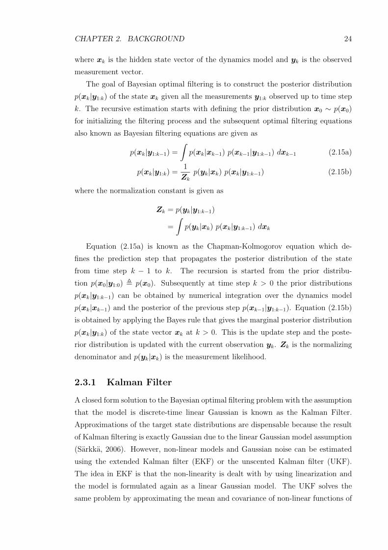
The goal of Bayesian optimal filtering is to construct the posterior distribution
p(xk|y1:k) of the state xk given all the measurements y1:k observed up to time step
k. The recursive estimation starts with defining the prior distribution x0 ∼ p(x0)
for initializing the filtering process and the subsequent optimal filtering equations
also known as Bayesian filtering equations are given as
p(xk|y1:k−1) =
∫p(xk|xk−1) p(xk−1|y1:k−1) dxk−1 (2.15a)
p(xk|y1:k) =1
Zk
p(yk|xk) p(xk|y1:k−1) (2.15b)
where the normalization constant is given as
Zk = p(yk|y1:k−1)
=
∫p(yk|xk) p(xk|y1:k−1) dxk
Equation (2.15a) is known as the Chapman-Kolmogorov equation which de-
fines the prediction step that propagates the posterior distribution of the state
from time step k − 1 to k. The recursion is started from the prior distribu-
tion p(x0|y1:0) , p(x0). Subsequently at time step k > 0 the prior distributions
p(xk|y1:k−1) can be obtained by numerical integration over the dynamics model
p(xk|xk−1) and the posterior of the previous step p(xk−1|y1:k−1). Equation (2.15b)
is obtained by applying the Bayes rule that gives the marginal posterior distribution
p(xk|y1:k) of the state vector xk at k > 0. This is the update step and the poste-
rior distribution is updated with the current observation yk. Zk is the normalizing
denominator and p(yk|xk) is the measurement likelihood.
2.3.1 Kalman Filter
A closed form solution to the Bayesian optimal filtering problem with the assumption
that the model is discrete-time linear Gaussian is known as the Kalman Filter.
Approximations of the target state distributions are dispensable because the result
of Kalman filtering is exactly Gaussian due to the linear Gaussian model assumption
(Sarkka, 2006). However, non-linear models and Gaussian noise can be estimated
using the extended Kalman filter (EKF) or the unscented Kalman filter (UKF).
The idea in EKF is that the non-linearity is dealt with by using linearization and
the model is formulated again as a linear Gaussian model. The UKF solves the
same problem by approximating the mean and covariance of non-linear functions of
CHAPTER 2. BACKGROUND 25
the Gaussian random variables in the model by propagating a set of sigma-points
through the non-linear functions (Julier and Uhlmann, 2004). A linear Gaussian
state-space model can be written in probabilistic notation as
p(xk|xk−1) ∼ N(xk|Ak−1xk−1,Qk)
p(yk|xk) ∼ N(yk|Hkxk,Rk).(2.17)
A more common notation used to represent linear Gaussian models in dynamic
estimation literature is
xk = Ak−1xk−1 + qk−1
yk = Hkxk + rk,(2.18)
where xk is the state, yk is the measurement, qk−1 ∼ N(0,Qk−1) is the process noise
and rk ∼ N(0,Rk) is the measurement noise. Ak−1 is the transition matrix and Hk
is the measurement model matrix.
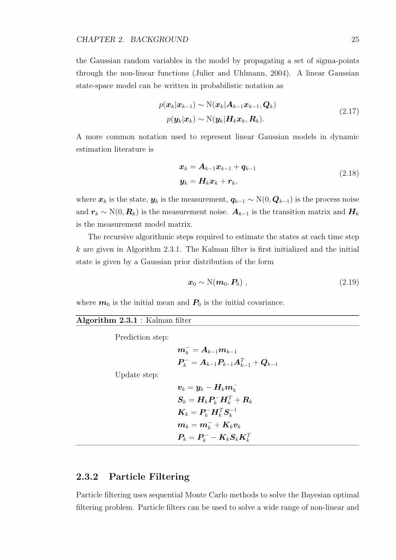
The recursive algorithmic steps required to estimate the states at each time step
k are given in Algorithm 2.3.1. The Kalman filter is first initialized and the initial
state is given by a Gaussian prior distribution of the form
x0 ∼ N(m0,P0) , (2.19)
where m0 is the initial mean and P0 is the initial covariance.
Algorithm 2.3.1 : Kalman filter
Prediction step:
m−k = Ak−1mk−1
P−k = Ak−1Pk−1ATk−1 +Qk−1
Update step:
vk = yk −Hkm−k
Sk = HkP−k H
Tk +Rk
Kk = P−k HTk S−1k
mk = m−k +Kkvk
Pk = P−k −KkSkKTk
2.3.2 Particle Filtering
Particle filtering uses sequential Monte Carlo methods to solve the Bayesian optimal
filtering problem. Particle filters can be used to solve a wide range of non-linear and
CHAPTER 2. BACKGROUND 26
non-Gaussian noise filtering problems since the method is based on approximating
the posterior distribution of the state variables via Monte Carlo. The posterior
distribution p(xk|y1:k) of the state xk at time step k is approximated as a set of
weighted Monte Carlo samples {(wk,x(i)k ) : i = 1, . . . , N}. The samples are drawn
from an importance distribution which approximates the target posterior distribu-
tion at each step.
Earlier algorithms of particle filtering known as sequential importance sampling
(SIS) suffered from the problem of degeneracy. This means that in certain conditions
almost all the particles have zero weights and only a few are non-zero. This problem
can be solved by introducing an additional resampling step to the SIS and in this
case the algorithm is known as sequential importance resampling (SIR) (Ristic et al.,
2004). The idea is to draw N new samples from a discrete distribution defined by
the weights and replace the old samples. Usually resampling is performed when it is
actually needed. One way of achieving this is by computing the effective number of
particles (samples) at each step and resampling if the effective number of particles
are less then a predefined threshold. This is termed as adaptive resampling which
actually consists of other methods as well like resampling after a predefined interval.
The effective number of particles can be calculated as
nEFF =1∑N
i=1(w(i)k )2
, (2.20)
where w(i)k is the normalized weight of particle i at time step k. Resampling can
be performed, for example, when nEFF < N/10 where N is the total number of
particles.
The performance of the SIR is highly dependent on the method of construct-
ing the importance distribution. The optimal importance distribution in terms of
variance is (Doucet et al., 2001; Ristic et al., 2004).
π(xk|xk−1,y1:k) = p(xk|xk−1,yk). (2.21)
In case the optimal distribution has a form that sampling from it directly is unfea-
sible then methods of linearisation can be used, for example, EKF, UKF or other
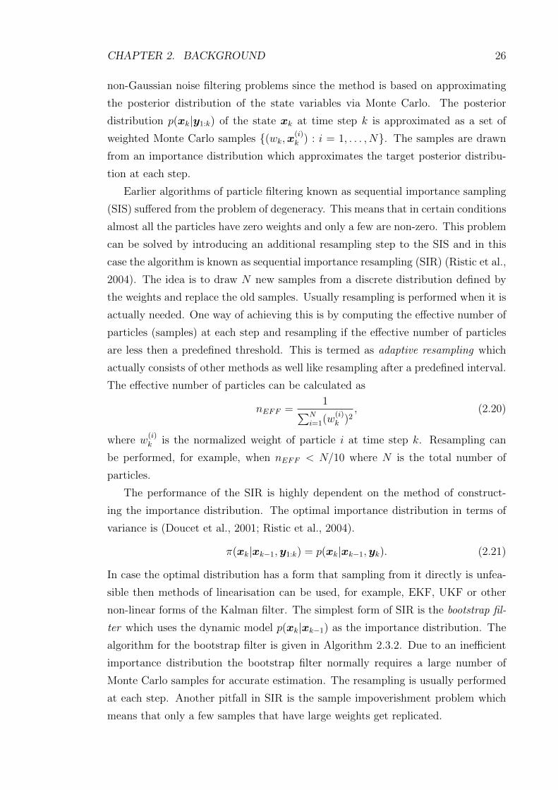
non-linear forms of the Kalman filter. The simplest form of SIR is the bootstrap fil-
ter which uses the dynamic model p(xk|xk−1) as the importance distribution. The
algorithm for the bootstrap filter is given in Algorithm 2.3.2. Due to an inefficient
importance distribution the bootstrap filter normally requires a large number of
Monte Carlo samples for accurate estimation. The resampling is usually performed
at each step. Another pitfall in SIR is the sample impoverishment problem which
means that only a few samples that have large weights get replicated.
CHAPTER 2. BACKGROUND 27
Algorithm 2.3.2 : Bootstrap filter
1: For each sample {x(i)k−1, i = 1, . . . , N}, draw new x
(i)k from
the dynamics model:
x(i)k ∼ p(xk|x(i)
k−1), i = 1, . . . , N .
2: Calculate the weights
w(i)k = p(yk|x(i)
k ), i = 1, . . . , N .
3: Normalize weights to sum to unity.
4: Perform resampling.
2.3.3 Rao-Blackwellized Particle Filtering
Sometimes it is possible to disintegrate the Bayesian filtering problem in to subprob-
lems, for example, estimation of a linear Gaussian part and approximation of a non-
linear part. The linear Gaussian part can be solved analytically, for example by using
the Kalman filter and the non-linear part can be solved by particle filtering. The
extended Kalman filter can also be used in case of slight non-linearities. This idea
of marginalizing the states of the dynamic system is known as Rao-Blackwellization.
The Rao-Blackellization improves the efficiency of the normal SIR by reducing the
number of Monte-Carlo samples required to approximate the target distribution.
This generates estimators with less variance as compared to standard Monte Carlo
sampling (Doucet et al., 2001; Ristic et al., 2004).
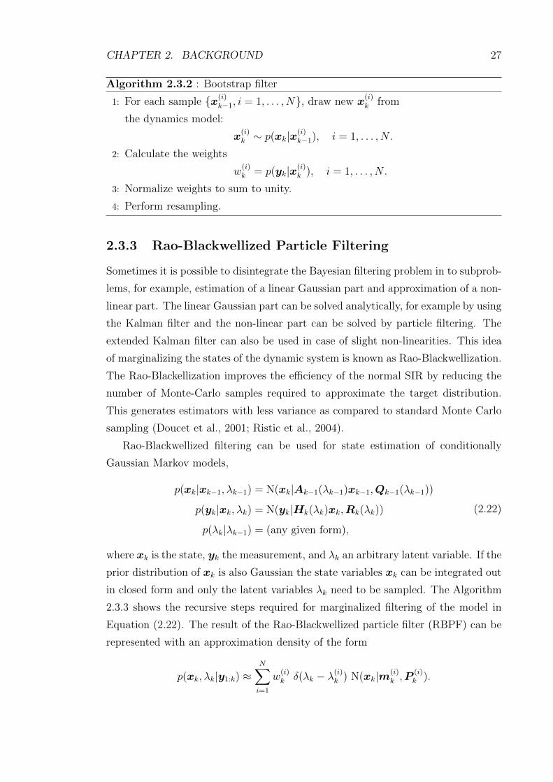
Rao-Blackwellized filtering can be used for state estimation of conditionally
Gaussian Markov models,
p(xk|xk−1, λk−1) = N(xk|Ak−1(λk−1)xk−1,Qk−1(λk−1))
p(yk|xk, λk) = N(yk|Hk(λk)xk,Rk(λk))
p(λk|λk−1) = (any given form),
(2.22)
where xk is the state, yk the measurement, and λk an arbitrary latent variable. If the
prior distribution of xk is also Gaussian the state variables xk can be integrated out
in closed form and only the latent variables λk need to be sampled. The Algorithm
2.3.3 shows the recursive steps required for marginalized filtering of the model in
Equation (2.22). The result of the Rao-Blackwellized particle filter (RBPF) can be
represented with an approximation density of the form
p(xk, λk|y1:k) ≈N∑i=1
w(i)k δ(λk − λ(i)k ) N(xk|m(i)
k ,P(i)k ).
CHAPTER 2. BACKGROUND 28
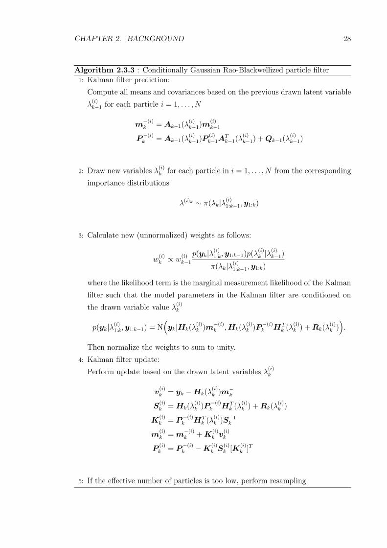
Algorithm 2.3.3 : Conditionally Gaussian Rao-Blackwellized particle filter
1: Kalman filter prediction:
Compute all means and covariances based on the previous drawn latent variable
λ(i)k−1 for each particle i = 1, . . . , N
m−(i)k = Ak−1(λ
(i)k−1)m
(i)k−1
P−(i)k = Ak−1(λ
(i)k−1)P
(i)k−1A
Tk−1(λ
(i)k−1) +Qk−1(λ
(i)k−1)
2: Draw new variables λ(i)k for each particle in i = 1, . . . , N from the corresponding
importance distributions
λ(i)k ∼ π(λk|λ(i)1:k−1,y1:k)
3: Calculate new (unnormalized) weights as follows:
w(i)k ∝ w
(i)k−1
p(yk|λ(i)1:k,y1:k−1)p(λ(i)k |λ
(i)k−1)
π(λk|λ(i)1:k−1,y1:k)
where the likelihood term is the marginal measurement likelihood of the Kalman
filter such that the model parameters in the Kalman filter are conditioned on
the drawn variable value λ(i)k
p(yk|λ(i)1:k,y1:k−1) = N(yk|Hk(λ
(i)k )m
−(i)k ,Hk(λ
(i)k )P
−(i)k HT
k (λ(i)k ) +Rk(λ
(i)k )).
Then normalize the weights to sum to unity.
4: Kalman filter update:
Perform update based on the drawn latent variables λ(i)k
v(i)k = yk −Hk(λ
(i)k )m−k
S(i)k = Hk(λ
(i)k )P
−(i)k HT
k (λ(i)k ) +Rk(λ
(i)k )
K(i)k = P
−(i)k HT
k (λ(i)k )S−1k
m(i)k = m
−(i)k +K
(i)k v
(i)k
P(i)k = P
−(i)k −K(i)
k S(i)k [K
(i)k ]T
5: If the effective number of particles is too low, perform resampling
CHAPTER 2. BACKGROUND 29
2.4 Target Tracking and Data Association
Target tracking is an application area of Bayesian optimal filtering. Target tracking
in abstract form has its origin in estimation theory (Bar-Shalom et al., 2001). The
definition of target tracking is case-dependent and it is based upon the type of so-
lution required to solve the underlying problem. Target tracking, in general, can be
defined as estimation of the state of a moving object (target) from noisy measure-
ments. Measurements are obtained from a single sensor or multiple sensors which
can be at fixed locations or moving platforms (Bar-Shalom and Li, 1995). Target
tracking is further classified to single target tracking and multiple target tracking.
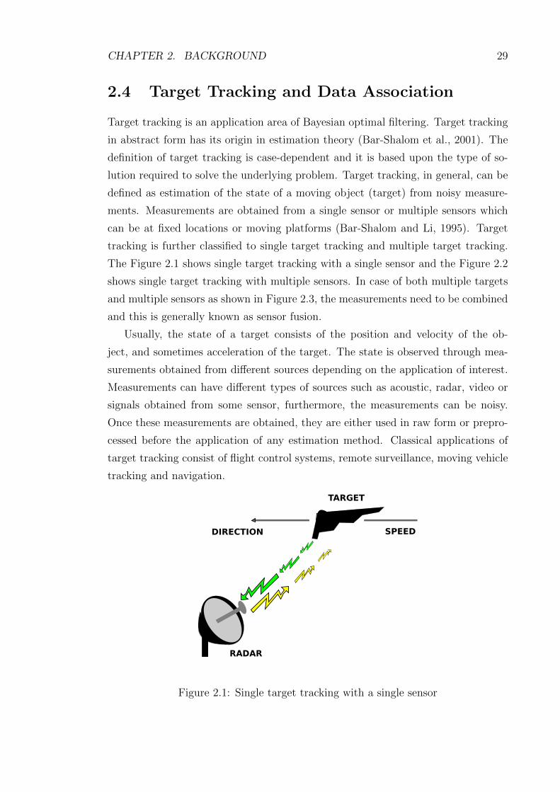
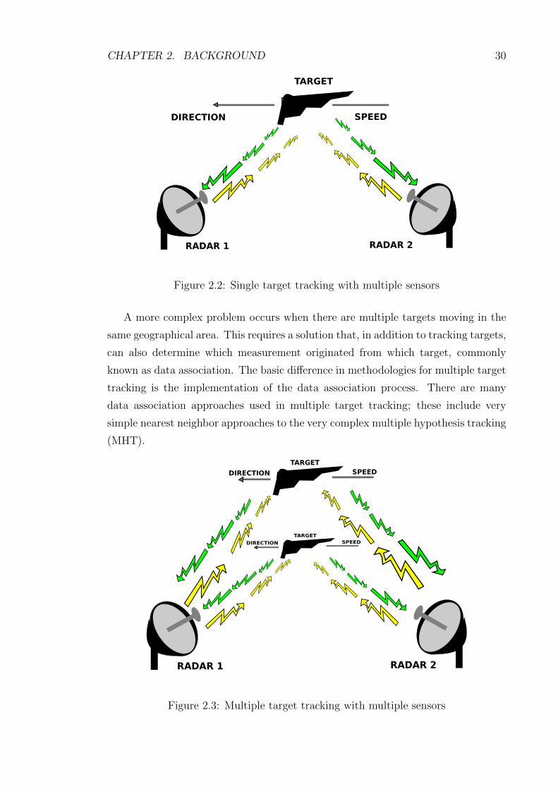
The Figure 2.1 shows single target tracking with a single sensor and the Figure 2.2
shows single target tracking with multiple sensors. In case of both multiple targets
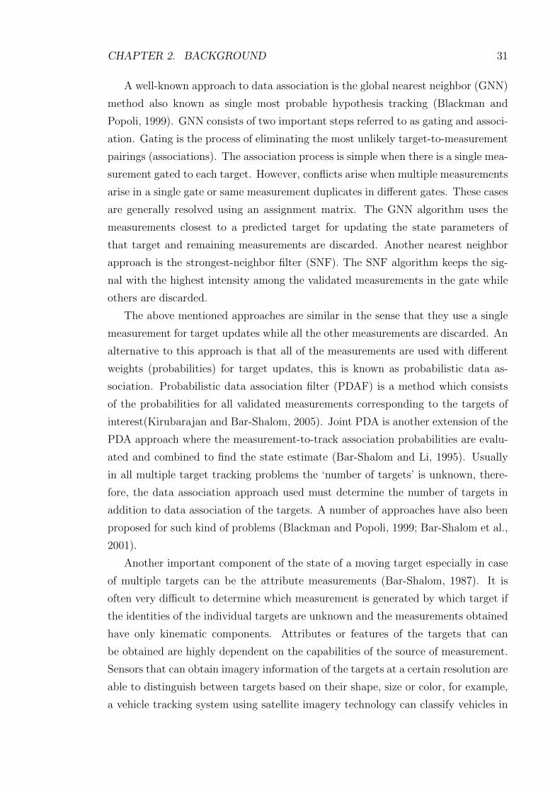
and multiple sensors as shown in Figure 2.3, the measurements need to be combined
and this is generally known as sensor fusion.
Usually, the state of a target consists of the position and velocity of the ob-
ject, and sometimes acceleration of the target. The state is observed through mea-
surements obtained from different sources depending on the application of interest.
Measurements can have different types of sources such as acoustic, radar, video or
signals obtained from some sensor, furthermore, the measurements can be noisy.
Once these measurements are obtained, they are either used in raw form or prepro-
cessed before the application of any estimation method. Classical applications of
target tracking consist of flight control systems, remote surveillance, moving vehicle
tracking and navigation.
RADAR
TARGET
DIRECTION SPEED
Figure 2.1: Single target tracking with a single sensor
CHAPTER 2. BACKGROUND 30
RADAR 1
TARGET
DIRECTION SPEED
RADAR 2
Figure 2.2: Single target tracking with multiple sensors
A more complex problem occurs when there are multiple targets moving in the
same geographical area. This requires a solution that, in addition to tracking targets,
can also determine which measurement originated from which target, commonly
known as data association. The basic difference in methodologies for multiple target
tracking is the implementation of the data association process. There are many
data association approaches used in multiple target tracking; these include very
simple nearest neighbor approaches to the very complex multiple hypothesis tracking
(MHT).
RADAR 1
TARGET
DIRECTION SPEED
RADAR 2
TARGET
DIRECTION SPEED
Figure 2.3: Multiple target tracking with multiple sensors
CHAPTER 2. BACKGROUND 31
A well-known approach to data association is the global nearest neighbor (GNN)
method also known as single most probable hypothesis tracking (Blackman and
Popoli, 1999). GNN consists of two important steps referred to as gating and associ-
ation. Gating is the process of eliminating the most unlikely target-to-measurement
pairings (associations). The association process is simple when there is a single mea-
surement gated to each target. However, conflicts arise when multiple measurements
arise in a single gate or same measurement duplicates in different gates. These cases
are generally resolved using an assignment matrix. The GNN algorithm uses the
measurements closest to a predicted target for updating the state parameters of
that target and remaining measurements are discarded. Another nearest neighbor
approach is the strongest-neighbor filter (SNF). The SNF algorithm keeps the sig-
nal with the highest intensity among the validated measurements in the gate while
others are discarded.
The above mentioned approaches are similar in the sense that they use a single
measurement for target updates while all the other measurements are discarded. An
alternative to this approach is that all of the measurements are used with different
weights (probabilities) for target updates, this is known as probabilistic data as-
sociation. Probabilistic data association filter (PDAF) is a method which consists
of the probabilities for all validated measurements corresponding to the targets of
interest(Kirubarajan and Bar-Shalom, 2005). Joint PDA is another extension of the
PDA approach where the measurement-to-track association probabilities are evalu-
ated and combined to find the state estimate (Bar-Shalom and Li, 1995). Usually
in all multiple target tracking problems the ‘number of targets’ is unknown, there-
fore, the data association approach used must determine the number of targets in
addition to data association of the targets. A number of approaches have also been
proposed for such kind of problems (Blackman and Popoli, 1999; Bar-Shalom et al.,
2001).
Another important component of the state of a moving target especially in case
of multiple targets can be the attribute measurements (Bar-Shalom, 1987). It is
often very difficult to determine which measurement is generated by which target if
the identities of the individual targets are unknown and the measurements obtained
have only kinematic components. Attributes or features of the targets that can
be obtained are highly dependent on the capabilities of the source of measurement.
Sensors that can obtain imagery information of the targets at a certain resolution are
able to distinguish between targets based on their shape, size or color, for example,
a vehicle tracking system using satellite imagery technology can classify vehicles in

CHAPTER 2. BACKGROUND 32
to different categories (e.g., car, truck, tractor). However, more restricted sources
that can only obtain kinematic measurements can use prior information about the
targets, for example, the maximum speed a target can attain or the maximum
turning angle possible. This is known as coarse kinematic information (Blackman
and Popoli, 1999). In case the coarse kinematic information is also similar among
all the targets then the data association process becomes even more difficult.
Chapter 3
Materials, Models and Methods
3.1 Data Sources
We have used an unconventional method of estimating animal abundance in compar-
ison to the standard methodology. This is mainly due to an unusual data collection
process. The data collection process is based on a reporting procedure that involves
multiple observers. The observations can be registered through websites, phones or
district game management offices. This is a voluntary task which can be performed
by anybody in Finland, for example, it is possible that somebody traveling via car
observes a carcass of a dead animal and reports to the district game management
office. The whole dataset consists of observations collected from almost every dis-
trict of Finland. This data collection is a continuous process which is supervised by
the Finnish Game and Fisheries Research Institute.
The dataset comprises mainly of four large carnivores: brown bear, wolf, lynx
and wolverine. The dataset also consists of index based data which is considered
to be more reliable information. The field work required to collect index based
samples is also a voluntary effort of around 1500 hunters all around Finland. These
volunteers have exceptional skill in finding and identifying marks left behind by
the animals. The observations are based on both direct sighting of the animal and
its remains (field-signs). Field-signs mainly consist of foot-prints, carcasses of dead
animal or prey, feces and habitual structures. One of the more important descriptors
in the data set is the number of cubs and one year olds which are assumed to be
following their mother. The foot print observations are also used to determine the
litter size and age of the animals. We briefly present the biological information and
animal tracks description that aid in the estimation of animal population.
33
CHAPTER 3. MATERIALS, MODELS AND METHODS 34
Brown Bear
A litter of 1− 3 and at times 4 cubs is born between January to March during the
hibernation period of a female bear. The cubs tend to follow the mother before
hibernating again the following winter and usually leave their mother in late spring
or summer of the next year. Males tend to disperse from their natal areas whereas
females usually establish home ranges nearby or overlapping their natal areas. Brown
bears are solitary animals and usually live their whole life in a single but large
habitual region. The home ranges of male bears are larger than those of female
bears. The annual home range of a female can be 60− 300 square kilometers while
that of a male can be over 1000 square kilometers (Katajisto, 2006).
Brown bears hibernate for 4 − 5 months which restricts the reliable sampling
period to merely 5− 6 months. Due to the long winter sleep a bear has to consume
sufficient food during spring and summer. This makes bears very active and they
tend to move around 10−30 kilometers a day in search of food. Bear foot prints can
be found quite apparently on sand and moss due to the huge weight of the animal.
Foot prints also assist in identifying other field signs for the presence of a bear such
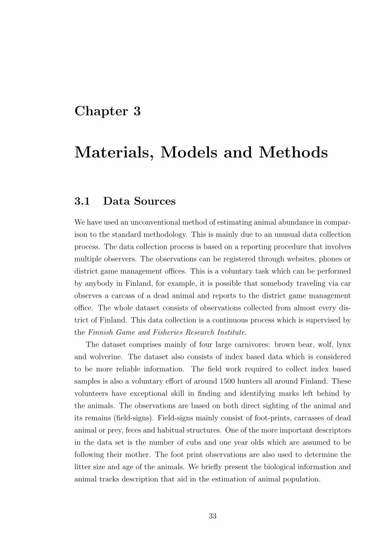
as broken tree branches, droppings and excavated anthills. Figure 3.1 shows a brown
bear1 and the foot print; the front foot or paw is 12−15cm in length and 10−18cm
in width while the rear foot is 18− 25cm in length and 10− 18cm in width.
Figure 3.1: Brown bear and foot sizes
Wolf
More often a pack of wolves is formed around a breeding alpha pair or the dominant
pair. Other members of the pack are usually 1 − 2 year olds of the same family.
1By Hillebrand, Steve [Public domain], via Wikimedia Commons.
http://creativecommons.org/licenses/by-sa/3.0/
CHAPTER 3. MATERIALS, MODELS AND METHODS 35
The female usually gives birth to a litter of 3− 6 cubs per year. The cubs are blind
and deaf when born and are nursed by the mother in a den for the first three weeks.
Wolves are highly social animals. All members of the pack hunt together and help
looking after the cubs . At the age of 1 − 2 years the young might leave the pack
and travel far from their birth place in search of their own territory and partner.
Wolf territories vary between 100− 1000 square kilometers. The territories are well
marked and strongly defended against other packs (Salvatori and Linnell, 2005).
Wolves travel 30− 50 kilometers a day but can also travel 160 kilometers if food
is scarce. Reliable descriptors for sampling are observations and field signs of wolf
packs rather than single observations since a single wolf is very hard to track unless
radio or GPS telemetry is used. Wolves move along roads, paths and tracks made
by humans and other animals. Their foot prints resemble to that of dogs but can
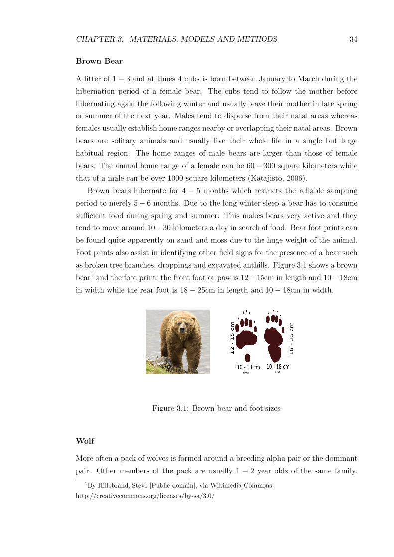
easily be distinguished by size and the tracks often tend to be in a straight path.
Figure 3.2 shows a wolf2 and the foot print; the length of the foot is 9− 10cm while
the width is 6.5− 10cm.
Figure 3.2: Wolf and foot size
Lynx
A female lynx usually gives birth to a litter of 2 − 3 kittens and more rarely 1 or
4 kittens are born. The lair is usually a hallow place with constant temperature
since the kittens are unable to regulate their body temperatures. The young begin
eating solid food only when they are at least three months old while they keep
suckling their mother for up to six months. Then the kittens leave the lair and start
following the mother. Initially unable to hunt they practice at prey captured by the
mother but learn rapidly and soon join the actual hunting. Lynx are solitary animals
2By Gary Kramer [Public domain], via Wikimedia Commons.
http://creativecommons.org/licenses/by-sa/3.0/
CHAPTER 3. MATERIALS, MODELS AND METHODS 36
except during the mating season which usually starts at the end of February to the
early April. Females usually give birth in May-June. The young might stay with
the mother at most for one year before dispersing. The home range and behavior
of lynx varies from region to region and primarily depends on the landscape and
density of prey (Breitenmoser, 2000). Generally, males travel more than females and
have larger home ranges that can vary from 120 to 1600 square kilometers. Females
with kittens can have a home range as small as 10 square kilometers but usually it
varies between 80− 500 square kilometers.
Lynx are mainly active after sunset and rest during the day time. It is observed
that distances covered during night time vary from 1 − 45 kilometers while males
travel more during the mating season. On the other hand females with kittens move
very short distances and stay in the proximity of a kill for several days. Lynx walk
at a steady pace but during hunting they can leap as long as 6− 8 meters. A Lynx
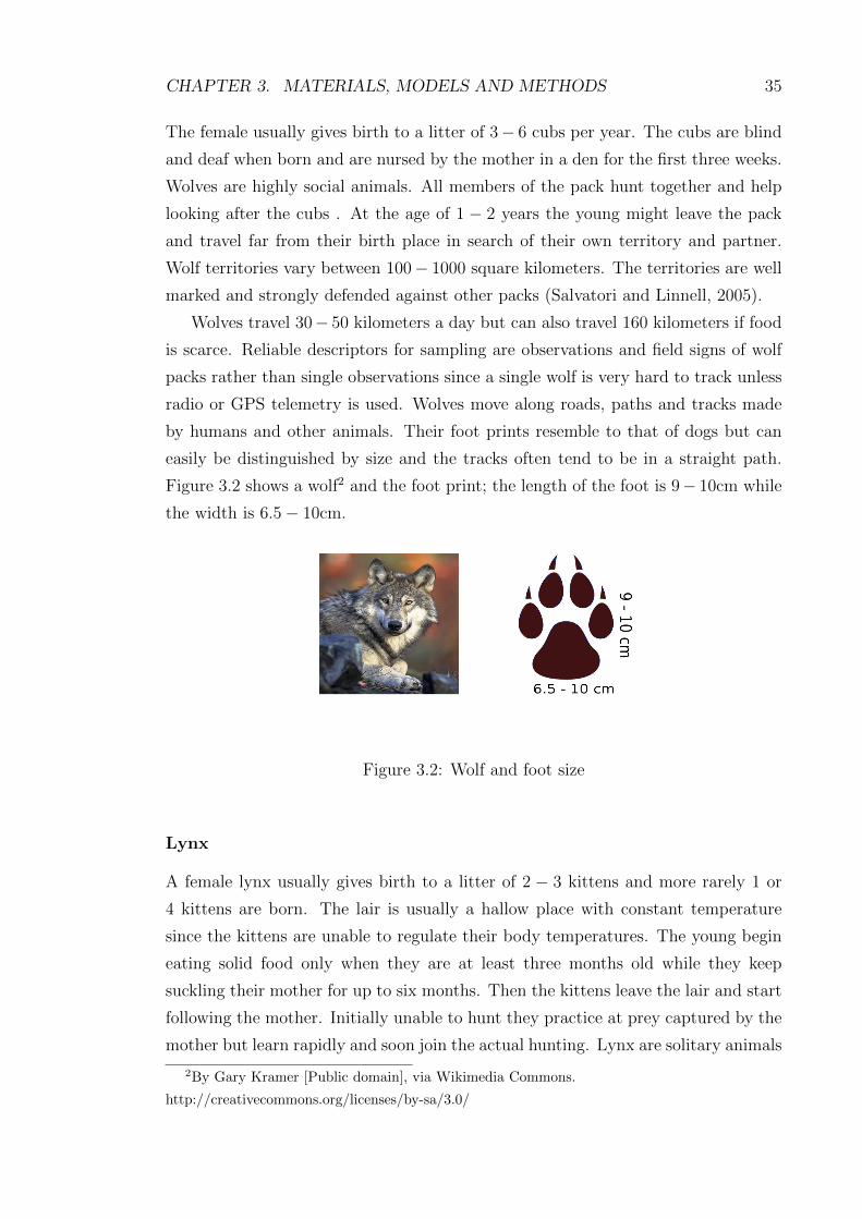
foot print resembles with that of a cat but it is usually larger. The thick fur around
the toes of a lynx makes rounded circles in snow. Figure 3.3 shows a lynx3 and the
foot print; the foot size is 7− 9cm in length and 6− 12cm in width.
Figure 3.3: Lynx and foot size
Wolverine
A female wolverine can usually have a litter of 2 − 3 cubs and occasionally 1 or
5 can be born. The cubs start walking with the mother at 9 − 10 weeks. The
mating season is from June to August while birth is in January to March. The
wolverine is generally a solitary animal but the social behavior and dispersal is
inadequately recorded. Usually the home range of a male can vary from 100− 500
square kilometers while that of a female can be 100− 200 square kilometers (Landa
et al., 2000).
3http://creativecommons.org/licenses/by-sa/2.0/de/deed.en
CHAPTER 3. MATERIALS, MODELS AND METHODS 37
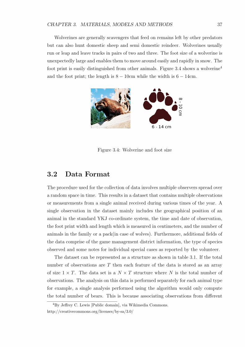
Wolverines are generally scavengers that feed on remains left by other predators
but can also hunt domestic sheep and semi domestic reindeer. Wolverines usually
run or leap and leave tracks in pairs of two and three. The foot size of a wolverine is
unexpectedly large and enables them to move around easily and rapidly in snow. The
foot print is easily distinguished from other animals. Figure 3.4 shows a wolverine4
and the foot print; the length is 8− 10cm while the width is 6− 14cm.
Figure 3.4: Wolverine and foot size
3.2 Data Format
The procedure used for the collection of data involves multiple observers spread over
a random space in time. This results in a dataset that contains multiple observations
or measurements from a single animal received during various times of the year. A
single observation in the dataset mainly includes the geographical position of an
animal in the standard YKJ co-ordinate system, the time and date of observation,
the foot print width and length which is measured in centimeters, and the number of
animals in the family or a pack(in case of wolves). Furthermore, additional fields of
the data comprise of the game management district information, the type of species
observed and some notes for individual special cases as reported by the volunteer.
The dataset can be represented as a structure as shown in table 3.1. If the total
number of observations are T then each feature of the data is stored as an array
of size 1 × T . The data set is a N × T structure where N is the total number of
observations. The analysis on this data is performed separately for each animal type
for example, a single analysis performed using the algorithm would only compute
the total number of bears. This is because associating observations from different
4By Jeffrey C. Lewis [Public domain], via Wikimedia Commons.
http://creativecommons.org/licenses/by-sa/3.0/
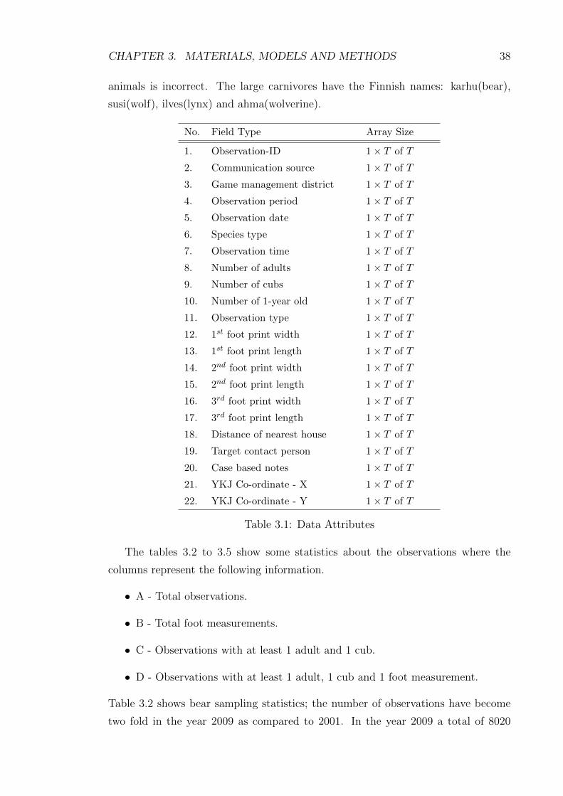
CHAPTER 3. MATERIALS, MODELS AND METHODS 38
animals is incorrect. The large carnivores have the Finnish names: karhu(bear),
susi(wolf), ilves(lynx) and ahma(wolverine).
No. Field Type Array Size
1. Observation-ID 1× T of T
2. Communication source 1× T of T
3. Game management district 1× T of T
4. Observation period 1× T of T
5. Observation date 1× T of T
6. Species type 1× T of T
7. Observation time 1× T of T
8. Number of adults 1× T of T
9. Number of cubs 1× T of T
10. Number of 1-year old 1× T of T
11. Observation type 1× T of T
12. 1st foot print width 1× T of T
13. 1st foot print length 1× T of T
14. 2nd foot print width 1× T of T
15. 2nd foot print length 1× T of T
16. 3rd foot print width 1× T of T
17. 3rd foot print length 1× T of T
18. Distance of nearest house 1× T of T
19. Target contact person 1× T of T
20. Case based notes 1× T of T
21. YKJ Co-ordinate - X 1× T of T
22. YKJ Co-ordinate - Y 1× T of T
Table 3.1: Data Attributes
The tables 3.2 to 3.5 show some statistics about the observations where the
columns represent the following information.
• A - Total observations.
• B - Total foot measurements.
• C - Observations with at least 1 adult and 1 cub.
• D - Observations with at least 1 adult, 1 cub and 1 foot measurement.
Table 3.2 shows bear sampling statistics; the number of observations have become
two fold in the year 2009 as compared to 2001. In the year 2009 a total of 8020
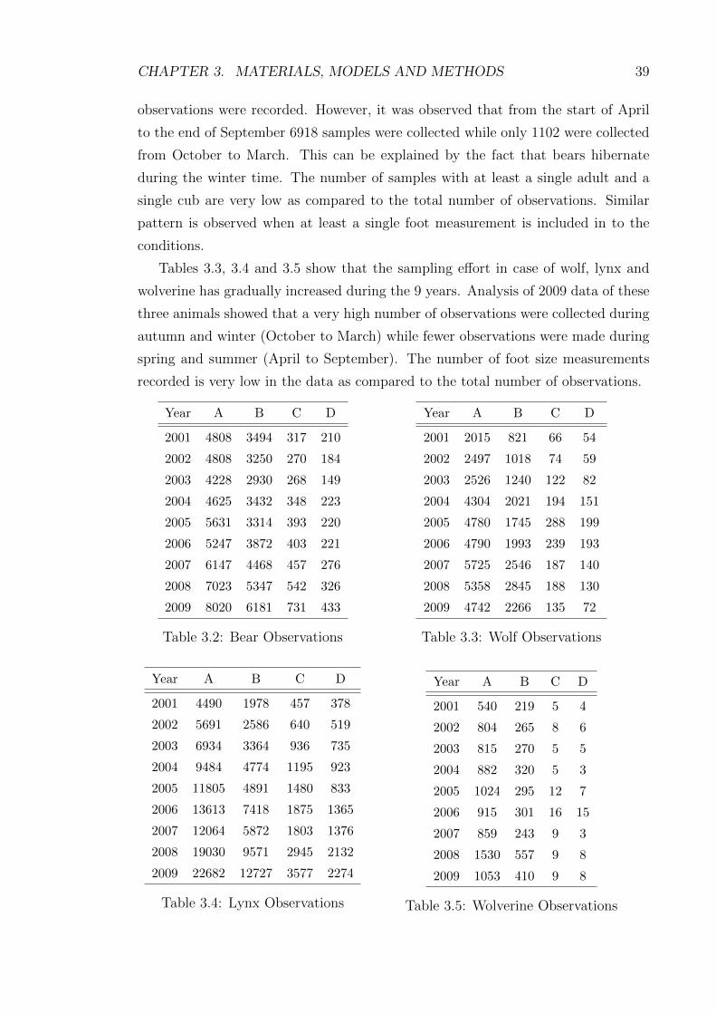
CHAPTER 3. MATERIALS, MODELS AND METHODS 39
observations were recorded. However, it was observed that from the start of April
to the end of September 6918 samples were collected while only 1102 were collected
from October to March. This can be explained by the fact that bears hibernate
during the winter time. The number of samples with at least a single adult and a
single cub are very low as compared to the total number of observations. Similar
pattern is observed when at least a single foot measurement is included in to the
conditions.
Tables 3.3, 3.4 and 3.5 show that the sampling effort in case of wolf, lynx and
wolverine has gradually increased during the 9 years. Analysis of 2009 data of these
three animals showed that a very high number of observations were collected during
autumn and winter (October to March) while fewer observations were made during
spring and summer (April to September). The number of foot size measurements
recorded is very low in the data as compared to the total number of observations.
Year A B C D
2001 4808 3494 317 210
2002 4808 3250 270 184
2003 4228 2930 268 149
2004 4625 3432 348 223
2005 5631 3314 393 220
2006 5247 3872 403 221
2007 6147 4468 457 276
2008 7023 5347 542 326
2009 8020 6181 731 433
Table 3.2: Bear Observations
Year A B C D
2001 2015 821 66 54
2002 2497 1018 74 59
2003 2526 1240 122 82
2004 4304 2021 194 151
2005 4780 1745 288 199
2006 4790 1993 239 193
2007 5725 2546 187 140
2008 5358 2845 188 130
2009 4742 2266 135 72
Table 3.3: Wolf Observations
Year A B C D
2001 4490 1978 457 378
2002 5691 2586 640 519
2003 6934 3364 936 735
2004 9484 4774 1195 923
2005 11805 4891 1480 833
2006 13613 7418 1875 1365
2007 12064 5872 1803 1376
2008 19030 9571 2945 2132
2009 22682 12727 3577 2274
Table 3.4: Lynx Observations
Year A B C D
2001 540 219 5 4
2002 804 265 8 6
2003 815 270 5 5
2004 882 320 5 3
2005 1024 295 12 7
2006 915 301 16 15
2007 859 243 9 3
2008 1530 557 9 8
2009 1053 410 9 8
Table 3.5: Wolverine Observations
CHAPTER 3. MATERIALS, MODELS AND METHODS 40
3.3 Model
We have used the state-space model framework as the basis for representing the
dynamic and measurement models. The dynamic animal movement models given as
linear stochastic differential equations (SDE) can be discretized in order to solve the
filtering problem. The discretization of linear SDE results in a discrete-time linear
Gaussian model, which is suitable for the Kalman filter. We can write a linear
(time-invariant) SDE in white noise notation as (Øksendal, 2003; Grewal et al.,
2001; Sarkka, 2006)dx(t)
dt= F x(t) +Lw(t) , (3.1)
where x(t) is a n−dimensional state vector at time t, F is a n×n constant coefficient
matrix, w(t) is a Gaussian white noise process with a spectral density matrix Qc
and L is a constant matrix.
Solution of linear SDE
We solve the linear stochastic differential equation given in Equation (3.1) by pre-
multiplying the integrating factor eF t in matrix exponential form as
e−F t(dx(t)
dt− F x(t)
)= e−F t
(Lw(t)
)=⇒ d
dt
(e−F t x(t)
)= e−F t
(Lw(t)
),
integrating the above expression between t0 and t∫ t
t0
d
dt
(e−F τ x(τ)
)=
∫ t
t0
e−F τ Lw(τ) dτ
=⇒ x(t) = eF (t−t0) x(t0) +
∫ t
t0
eF (t−τ)Lw(τ) dτ . (3.2)
The mean and covariance can be computed from Equation (3.2). The solution to
the linear SDE is a Gaussian process with mean and covariance (Grewal et al., 2001)
m(t) = exp(F (t− t0))x(t0) (3.3)
P (t) = exp(F (t− t0))P (t0) exp(F (t− t0))T
+
∫ t
t0
exp(F (t− t0))LQcLT exp(F (t− t0))T dt0 , (3.4)
where x(t0) ∼ N(m(t0),P (t0)) and exp(.) is the matrix exponential function.
CHAPTER 3. MATERIALS, MODELS AND METHODS 41
Discretization
Because t0 in Equations (3.3) and (3.4) is arbitrary, we can also express the solution
in recursive form as follows:
m(tk) = exp(F (tk − tk−1))︸ ︷︷ ︸Ak−1
m(tk−1) (3.5)
P (tk) = exp(F (tk − tk−1))︸ ︷︷ ︸Ak−1
P (tk−1) exp(F (tk − tk−1))T︸ ︷︷ ︸AT
k−1
+
∫ tk
tk−1
exp(F (tk − tk−1))LQcLT exp(F (tk − tk−1))T dtk−1︸ ︷︷ ︸
Qk−1
, (3.6)
where x(tk−1) ∼ N(m(tk−1),P (tk−1)) and exp(.) is the matrix exponential function.
Thus the mean and covariance of the solution in Equations (3.3) and (3.4) at discrete
instances t1, t2, . . . are given by the recursive equations;
mk = Ak−1mk−1 (3.7)
Pk = Ak−1Pk−1ATk−1 + Qk−1 , (3.8)
where mk = m(tk) and Pk = P (tk). By comparing to Algorithm 2.3.1, we can see
that this is exactly the Kalman filter prediction step.
3.4 Method
We have used the Rao-Blackwellized Monte Carlo data association (RBMCDA) al-
gorithm, designed to solve the problem of data association in case of both ‘a known
number of targets’ and ‘an unknown number of targets’, presented in (Sarkka et al.,
2007). The idea of Rao-Blackwellization is implemented in such a way that the
individual states of the targets is estimated analytically, for example, Kalman filter
is used when the dynamic and measurement models are linear Gaussian. State esti-
mation is conditional on the data associations, which are sampled using sequential
importance resampling (SIR).
RBMCDA with Known Number of Targets
Consider the state-space model given as
xj,k = Aj,k−1xj,k−1 + qj,k−1
yk = Hj,kxj,k + rj,k(3.9)
CHAPTER 3. MATERIALS, MODELS AND METHODS 42
where number of targets j = 1, . . . , T and the process noise qj,k−1 and measurement
noise rj,k terms are zero mean with covariance matricesQj,k−1 andRj,k, respectively.
qj,k−1 ∼ N(0,Qj,k−1)
rj,k ∼ N(0,Rj,k) .(3.10)
The problem is to estimate the states of T targets from noisy and cluttered mea-
surements y1:k. This is possible only if the sources of the measurements can be
distinguished, that is, which measurement has originated from which target. The
measurements can also be ‘clutter measurements’. Clutter or false alarm refers to
the measurements that originate from some other source than from the targets that
we are tracking. Therefore, a single measurement at time step k can originate from
one of two different sources; one of the known targets j = 1, . . . , T or clutter j = 0.
The RBMCDA algorithm basically involves the same steps as already described
in the Algorithm 2.3.3. Because the latent variable is discrete, we can use the
optimal importance distribution in the Rao-Blackwellized particle filter for solving
the data association problem. The clutter is assumed to be uniformly distributed on
the observation area with volume V and thus the probability density of a cluttered
measurement yk is given as
p(yk|ck = 0) = 1/V, (3.11)
where ck is the data association indicator or latent variable as in the case of the
conditionally Gaussian Markov models. The data association indicator has the value
ck = j for targets j = 1, . . . , T and the probability of the measurement originated
from a target is same as the Kalman filter likelihood given by
p(yk|xj,k, ck = j) = N(yk|Hj,kxj,k,Rj,k) , (3.12)
where the measurement model matrices Hj,k and Rj,k can be different for each
target. The target and clutter association priors are assumed to be known and
given by p(ck|c1:k−1), for example, when there are only 2 targets and the clutter
density is 50% the prior probabilities would be
p(ck = 0) = 0.5
p(ck = 1) = 0.25
p(ck = 2) = 0.25 .
(3.13)
The optimal distribution required for the SIR can now be written as p(ck|y1:k, c1:k−1).
CHAPTER 3. MATERIALS, MODELS AND METHODS 43
For the implementation of RBMCDA algorithm with N number of particles, the
algorithm state stores and updates
particle 1 : {c(1)1,k,m(1)1,k,P
(1)1,k , c
(1)2,k,m
(1)2,k,P
(1)2,k , . . . , c
(1)T,k,m
(1)T,k,P
(1)T,k, w
(1)k }
particle 2 : {c(2)1,k,m(2)1,k,P
(2)1,k , c
(2)2,k,m
(2)2,k,P
(2)2,k , . . . , c
(2)T,k,m
(2)T,k,P
(2)T,k, w
(2)k }
...
particle N : {c(N)1,k ,m
(N)1,k ,P
(N)1,k , c
(N)2,k ,m
(N)2,k ,P
(N)2,k , . . . , c
(N)T,k ,m
(N)T,k ,P
(N)T,k , w
(N)k } ,
where c(i)1:T,k are the data association indicators for the targets which can have integer
values 0, . . . , T , and m(i)1:T,k,P
(i)1:T,k are the means and covariances of the targets and
w(i)k is the importance weight of each particle i = 1, . . . , N .
The optimal importance distributions for N particles are p(ck|y1:k, c(i)1:k−1), where
i = 1, . . . , N . The following steps have to be performed in order to sample from the
optimal distribution at each step k,
1. Compute the clutter association probability as
π(i)0 = p(yk|c(i)k = 0,y1:k−1, c
(i)1:k−1)p(c
(i)k = 0)
2. Compute the target association probability for each target j = 1, . . . , T as
π(i)j = p(yk|c(i)k = j,y1:k−1, c
(i)1:k−1)p(c
(i)k = j)
3. Normalize the importance distribution as
π(i)j =
π(i)j∑T
t=0 π(i)t
, j = 0, . . . , T
4. Sample new associations to targets and clutter as
• Draw c(i)k = 0 with probability π
(i)0
• Draw c(i)k = 1 with probability π
(i)1
• . . .
• Draw c(i)k = T with probability π
(i)T .
RBMCDA with Unknown Number of Targets
Again the aim is to estimate the state of the targets and the same model can be
considered as given in Equation (3.9). However, it is assumed that a very large
and constant number of targets T∞ are always available to be detected but only a
varying number of them are visible or alive. Therefore, a single measurement at
time step k can be assumed to be originated from one of three different sources;
CHAPTER 3. MATERIALS, MODELS AND METHODS 44
• one of the existing targets j = 1, . . . , T .
• a new target j = T + 1.
• clutter j = 0.
The probability density of a cluttered measurement is the same as in Equation (3.11)
and the the probability of a measurement originated from an existing target is the
same as in Equation (3.12). However, the probability of a measurement originated
from a new target would be the Kalman filter likelihood which can be computed given
the initial mean m0 and initial process noise covariance P0, using the measurement
likelihood
p(yk|x0, ck = j) = N(yk|Hj=T+1,kx0,Rj=T+1,k) , (3.14)
where ck is the data association indicator which has a value j = T + 1 and the
measurement model matrices Hj=T+1,k and Rj=T+1,k can be different for the new
target. The association of a measurement to a new target is called a birth. The
target and clutter associations probabilities can be modeled as
p(bk, ck|c1:k−1) =pb , event(1)
(1− pb)p(ck|c1:k−1) , event(2)
0 , event(3)
(3.15)
where event(1) indicates the birth of a new target which has a probability pb, event(2)
indicates the probabilities of association to an existing target or clutter and all other
events have zero probability. Each target has a life time td after getting associated
to a measurement. The time to death probability density is given by
td ∼ p(td), (3.16)
which can be, for example, an exponential or gamma distribution.
Similar steps can be followed for the implementation of RBMCDA with ‘an
unknown number of targets’ as in the case of ‘a known number of targets’. The
algorithm state stores and updates
particle 1 : {e(1)k , c(1)1,k,m
(1)1,k,P
(1)1,k , c
(1)2,k,m
(1)2,k,P
(1)2,k , . . . , c
(1)T∞,k
,m(1)T∞,k
,P(1)T∞,k
, w(1)k }
particle 2 : {e(2)k , c(2)1,k,m
(2)1,k,P
(2)1,k , c
(2)2,k,m
(2)2,k,P
(2)2,k , . . . , c
(2)T∞,k
,m(2)T∞,k
,P(2)T∞,k
, w(2)k }
...
particle N : {e(N)k , c
(N)1,k ,m
(N)1,k ,P
(N)1,k , c
(N)2,k ,m
(N)2,k ,P
(N)2,k , . . . , c
(N)T∞,k
,m(N)T∞,k
P(N)T∞,k
, w(N)k } ,

CHAPTER 3. MATERIALS, MODELS AND METHODS 45
where e(i)k is the life indicator vector of length T
(i)k , c
(i)1:T,k are the data association
indicators for the targets which can have integer values 0, . . . , T(i)k , and m
(i)1:T,k,P
(i)1:T,k
are the means and covariances of the targets and w(i)k is the importance weight of
each particle i = 1, . . . , N . The number of targets T(i)k in each particle i = 1, . . . , N
at time step k can be different and the expected number of targets at time step k
can be computed by a weighted sum over the particles as
Tk =N∑i=1
w(i)k T
(i)k . (3.17)
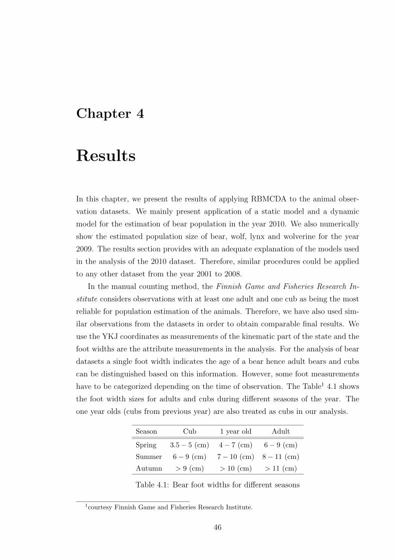
Chapter 4
Results
In this chapter, we present the results of applying RBMCDA to the animal obser-
vation datasets. We mainly present application of a static model and a dynamic
model for the estimation of bear population in the year 2010. We also numerically
show the estimated population size of bear, wolf, lynx and wolverine for the year
2009. The results section provides with an adequate explanation of the models used
in the analysis of the 2010 dataset. Therefore, similar procedures could be applied
to any other dataset from the year 2001 to 2008.
In the manual counting method, the Finnish Game and Fisheries Research In-
stitute considers observations with at least one adult and one cub as being the most
reliable for population estimation of the animals. Therefore, we have also used sim-
ilar observations from the datasets in order to obtain comparable final results. We
use the YKJ coordinates as measurements of the kinematic part of the state and the
foot widths are the attribute measurements in the analysis. For the analysis of bear
datasets a single foot width indicates the age of a bear hence adult bears and cubs
can be distinguished based on this information. However, some foot measurements
have to be categorized depending on the time of observation. The Table1 4.1 shows
the foot width sizes for adults and cubs during different seasons of the year. The
one year olds (cubs from previous year) are also treated as cubs in our analysis.
Season Cub 1 year old Adult
Spring 3.5− 5 (cm) 4− 7 (cm) 6− 9 (cm)
Summer 6− 9 (cm) 7− 10 (cm) 8− 11 (cm)
Autumn > 9 (cm) > 10 (cm) > 11 (cm)
Table 4.1: Bear foot widths for different seasons
1courtesy Finnish Game and Fisheries Research Institute.
46
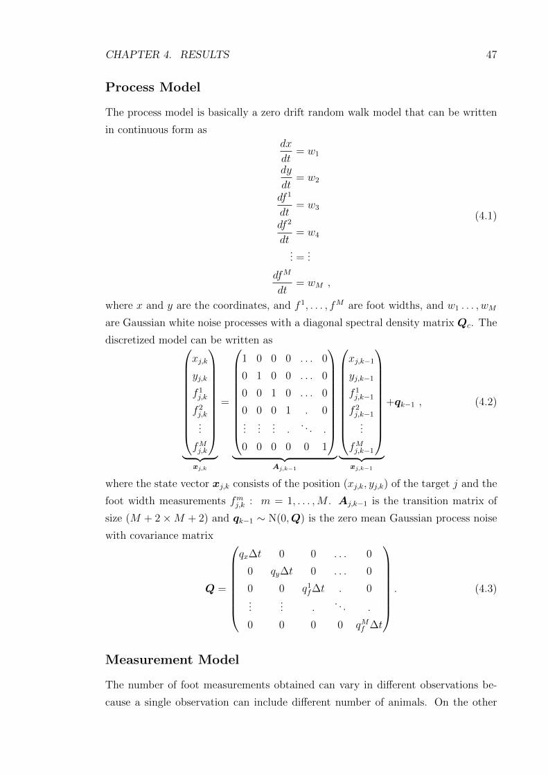
CHAPTER 4. RESULTS 47
Process Model
The process model is basically a zero drift random walk model that can be written
in continuous form as
dx
dt= w1
dy
dt= w2
df 1
dt= w3
df 2
dt= w4
... =...
dfM
dt= wM ,
(4.1)
where x and y are the coordinates, and f 1, . . . , fM are foot widths, and w1 . . . , wM
are Gaussian white noise processes with a diagonal spectral density matrix Qc. The
discretized model can be written as
xj,k
yj,k
f 1j,k
f 2j,k...
fMj,k
︸ ︷︷ ︸
xj,k
=
1 0 0 0 . . . 0
0 1 0 0 . . . 0
0 0 1 0 . . . 0
0 0 0 1 . 0...
...... .
. . . .
0 0 0 0 0 1
︸ ︷︷ ︸
Aj,k−1
xj,k−1
yj,k−1
f 1j,k−1
f 2j,k−1...
fMj,k−1
︸ ︷︷ ︸
xj,k−1
+qk−1 , (4.2)
where the state vector xj,k consists of the position (xj,k, yj,k) of the target j and the
foot width measurements fmj,k : m = 1, . . . ,M . Aj,k−1 is the transition matrix of
size (M + 2×M + 2) and qk−1 ∼ N(0,Q) is the zero mean Gaussian process noise
with covariance matrix
Q =
qx∆t 0 0 . . . 0
0 qy∆t 0 . . . 0
0 0 q1f∆t . 0...
... .. . . .
0 0 0 0 qMf ∆t
. (4.3)
Measurement Model
The number of foot measurements obtained can vary in different observations be-
cause a single observation can include different number of animals. On the other
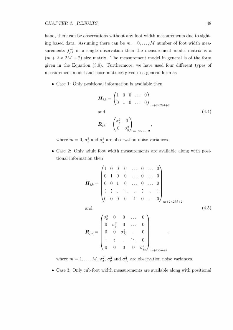
CHAPTER 4. RESULTS 48
hand, there can be observations without any foot width measurements due to sight-
ing based data. Assuming there can be m = 0, . . . ,M number of foot width mea-
surements fmj,k in a single observation then the measurement model matrix is a
(m + 2 × 2M + 2) size matrix. The measurement model in general is of the form
given in the Equation (3.9). Furthermore, we have used four different types of
measurement model and noise matrices given in a generic form as
• Case 1: Only positional information is available then
Hj,k =
(1 0 0 . . . 0
0 1 0 . . . 0
)m+2×2M+2
and
Rj,k =
(σ2x 0
0 σ2y
)m+2×m+2
,
(4.4)
where m = 0, σ2x and σ2
y are observation noise variances.
• Case 2: Only adult foot width measurements are available along with posi-
tional information then
Hj,k =
1 0 0 0 . . . 0 . . . 0
0 1 0 0 . . . 0 . . . 0
0 0 1 0 . . . 0 . . . 0...
... .. . . .
... ....
0 0 0 0 1 0 . . . 0
m+2×2M+2
and
Rj,k =
σ2x 0 0 . . . 0
0 σ2y 0 . . . 0
0 0 σ2fa
. 0...
... .. . . 0
0 0 0 0 σ2fa
m+2×m+2
,
(4.5)
where m = 1, . . . ,M , σ2x, σ
2y and σ2
faare observation noise variances.
• Case 3: Only cub foot width measurements are available along with positional
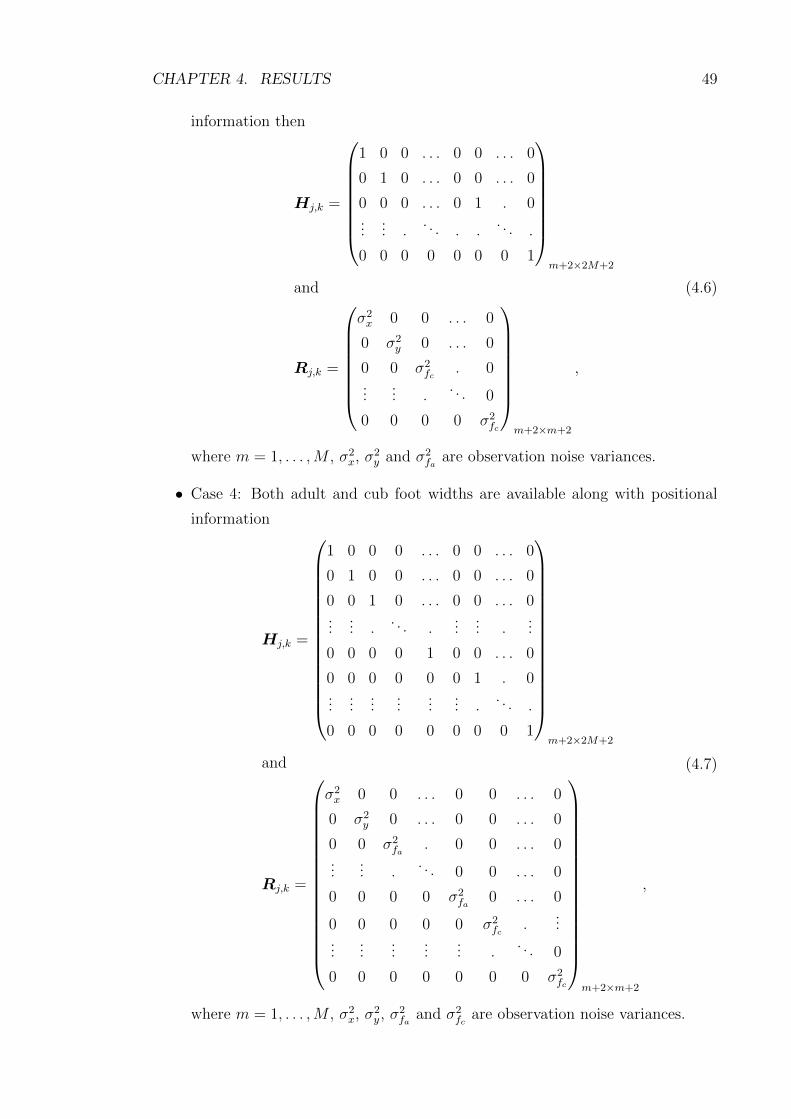
CHAPTER 4. RESULTS 49
information then
Hj,k =
1 0 0 . . . 0 0 . . . 0
0 1 0 . . . 0 0 . . . 0
0 0 0 . . . 0 1 . 0...
... .. . . . .
. . . .
0 0 0 0 0 0 0 1
m+2×2M+2
and (4.6)
Rj,k =
σ2x 0 0 . . . 0
0 σ2y 0 . . . 0
0 0 σ2fc
. 0...
... .. . . 0
0 0 0 0 σ2fc
m+2×m+2
,
where m = 1, . . . ,M , σ2x, σ
2y and σ2
faare observation noise variances.
• Case 4: Both adult and cub foot widths are available along with positional
information
Hj,k =
1 0 0 0 . . . 0 0 . . . 0
0 1 0 0 . . . 0 0 . . . 0
0 0 1 0 . . . 0 0 . . . 0...
... .. . . .
...... .
...
0 0 0 0 1 0 0 . . . 0
0 0 0 0 0 0 1 . 0...
......
......
... .. . . .
0 0 0 0 0 0 0 0 1
m+2×2M+2
and
Rj,k =
σ2x 0 0 . . . 0 0 . . . 0
0 σ2y 0 . . . 0 0 . . . 0
0 0 σ2fa
. 0 0 . . . 0...
... .. . . 0 0 . . . 0
0 0 0 0 σ2fa
0 . . . 0
0 0 0 0 0 σ2fc
....
......
......
... .. . . 0
0 0 0 0 0 0 0 σ2fc
m+2×m+2
,
(4.7)
where m = 1, . . . ,M , σ2x, σ
2y , σ
2fa
and σ2fc
are observation noise variances.
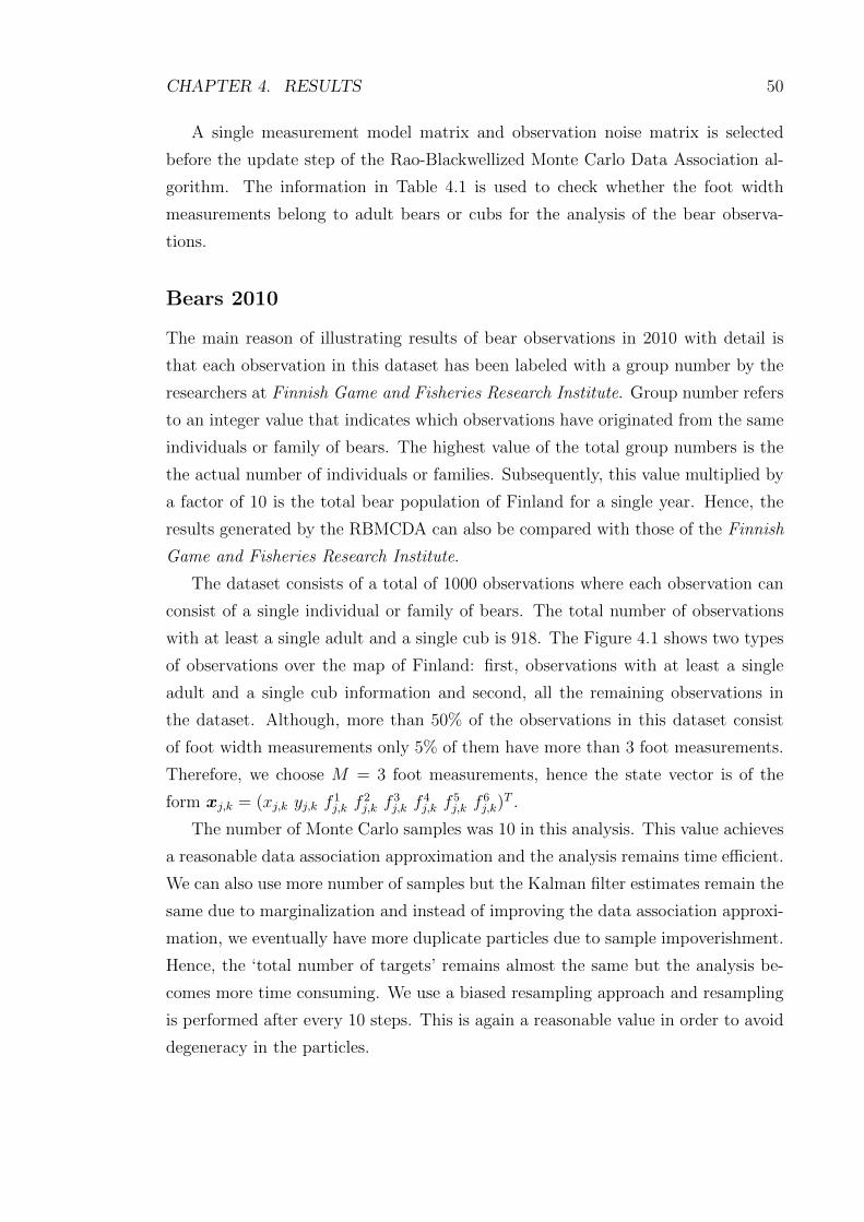
CHAPTER 4. RESULTS 50
A single measurement model matrix and observation noise matrix is selected
before the update step of the Rao-Blackwellized Monte Carlo Data Association al-
gorithm. The information in Table 4.1 is used to check whether the foot width
measurements belong to adult bears or cubs for the analysis of the bear observa-
tions.
Bears 2010
The main reason of illustrating results of bear observations in 2010 with detail is
that each observation in this dataset has been labeled with a group number by the
researchers at Finnish Game and Fisheries Research Institute. Group number refers
to an integer value that indicates which observations have originated from the same
individuals or family of bears. The highest value of the total group numbers is the
the actual number of individuals or families. Subsequently, this value multiplied by
a factor of 10 is the total bear population of Finland for a single year. Hence, the
results generated by the RBMCDA can also be compared with those of the Finnish
Game and Fisheries Research Institute.
The dataset consists of a total of 1000 observations where each observation can
consist of a single individual or family of bears. The total number of observations
with at least a single adult and a single cub is 918. The Figure 4.1 shows two types
of observations over the map of Finland: first, observations with at least a single
adult and a single cub information and second, all the remaining observations in
the dataset. Although, more than 50% of the observations in this dataset consist
of foot width measurements only 5% of them have more than 3 foot measurements.
Therefore, we choose M = 3 foot measurements, hence the state vector is of the
form xj,k = (xj,k yj,k f1j,k f
2j,k f
3j,k f
4j,k f
5j,k f
6j,k)
T .
The number of Monte Carlo samples was 10 in this analysis. This value achieves
a reasonable data association approximation and the analysis remains time efficient.
We can also use more number of samples but the Kalman filter estimates remain the
same due to marginalization and instead of improving the data association approxi-
mation, we eventually have more duplicate particles due to sample impoverishment.
Hence, the ‘total number of targets’ remains almost the same but the analysis be-
comes more time consuming. We use a biased resampling approach and resampling
is performed after every 10 steps. This is again a reasonable value in order to avoid
degeneracy in the particles.
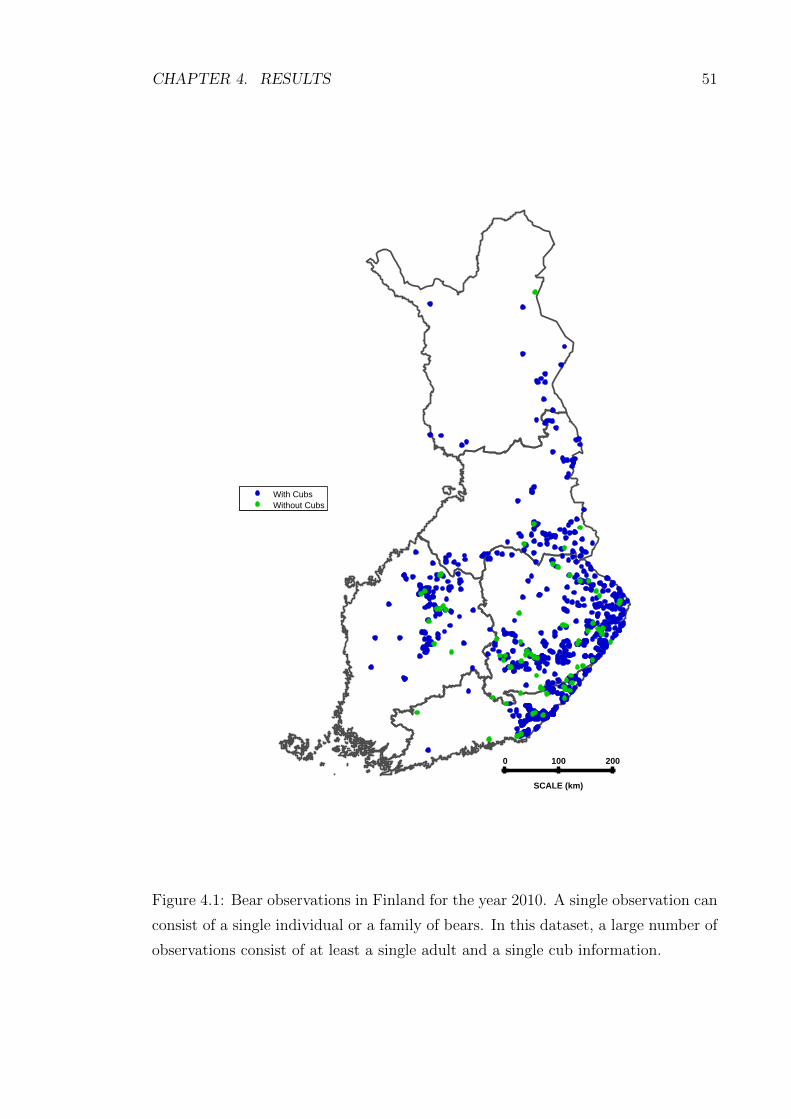
CHAPTER 4. RESULTS 51
SCALE (km)
0 100 200
With CubsWithout Cubs
Figure 4.1: Bear observations in Finland for the year 2010. A single observation can
consist of a single individual or a family of bears. In this dataset, a large number of
observations consist of at least a single adult and a single cub information.
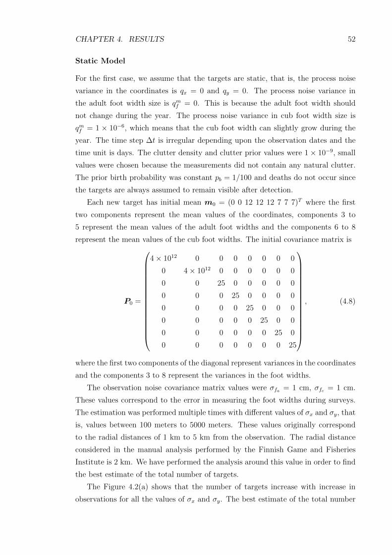
CHAPTER 4. RESULTS 52
Static Model
For the first case, we assume that the targets are static, that is, the process noise
variance in the coordinates is qx = 0 and qy = 0. The process noise variance in
the adult foot width size is qmf = 0. This is because the adult foot width should
not change during the year. The process noise variance in cub foot width size is
qmf = 1 × 10⁻⁶, which means that the cub foot width can slightly grow during the
year. The time step ∆t is irregular depending upon the observation dates and the
time unit is days. The clutter density and clutter prior values were 1× 10⁻⁹, small
values were chosen because the measurements did not contain any natural clutter.
The prior birth probability was constant pb = 1/100 and deaths do not occur since
the targets are always assumed to remain visible after detection.
Each new target has initial mean m0 = (0 0 12 12 12 7 7 7)T where the first
two components represent the mean values of the coordinates, components 3 to
5 represent the mean values of the adult foot widths and the components 6 to 8
represent the mean values of the cub foot widths. The initial covariance matrix is
P0 =
4× 10¹² 0 0 0 0 0 0 0
0 4× 10¹² 0 0 0 0 0 0
0 0 25 0 0 0 0 0
0 0 0 25 0 0 0 0
0 0 0 0 25 0 0 0
0 0 0 0 0 25 0 0
0 0 0 0 0 0 25 0
0 0 0 0 0 0 0 25
, (4.8)
where the first two components of the diagonal represent variances in the coordinates
and the components 3 to 8 represent the variances in the foot widths.
The observation noise covariance matrix values were σfa = 1 cm, σfc = 1 cm.
These values correspond to the error in measuring the foot widths during surveys.
The estimation was performed multiple times with different values of σx and σy, that
is, values between 100 meters to 5000 meters. These values originally correspond
to the radial distances of 1 km to 5 km from the observation. The radial distance
considered in the manual analysis performed by the Finnish Game and Fisheries
Institute is 2 km. We have performed the analysis around this value in order to find
the best estimate of the total number of targets.
The Figure 4.2(a) shows that the number of targets increase with increase in
observations for all the values of σx and σy. The best estimate of the total number
CHAPTER 4. RESULTS 53
0 200 400 600 800 10000
100
200
300
400
500
600
Observations
(a)
True number of targets
Estimated number of targets
0 200 400 600 800 10000
50
100
150
200
Observations
(b)
True number of targets
Best Estimate
0 50 100 150 2000
10
20
30
40
50
Groups/Targets
Ob
serv
ation
s/M
ea
sure
me
nts
(c)
0 50 100 150 2000
10
20
30
40
50
Groups/Targets
Ob
serv
ation
s/M
ea
sure
me
nts
(d)
Figure 4.2: (a) Different estimated number of targets in time, (b) Best estimate of
the total number of targets, (c) True Group distribution, (d) Group distribution for
the best estimate of the total number of targets.
of targets was found with σx = 2400 meters and σy = 2400 meters shown in Figure
4.2(b). The Figure 4.2(c) shows the true distribution of groups while Figure 4.2(d)
shows the estimated group distribution of the best estimate. The groups in the esti-
mated group distribution have slightly higher number of observations as compared
to the true groups because many observations in the dataset were unlabeled. The
results of the data association can also be visualized on the map of Finland as shown
in Figure 4.3. It is observed that the true groups are more overlapping as compared
to the estimated groups which have more discrete boundaries. Three different ex-
amples are illustrated in the Figure 4.4, where (a), (c) and (e) show the true groups
at three different locations in Finland, and (b), (d), (f) show the corresponding data
associations obtained by RBMCDA.
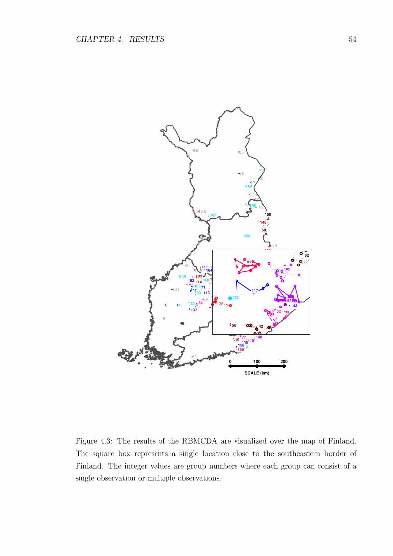
CHAPTER 4. RESULTS 54
SCALE (km)
0 100 200
1
2
3
4
5
6
7
8
9
10
11
12 13
14
15
16
17
18
19 20
2122
23
24
25
26
27
28
29
30
3132
33
34
35
36
37
38
39
40
41 42
43
44
45
46
47
48
49
50
51
5253
54
55
56
57
58
59
60
61
62
63
64
65
66
67
68
69
70
71
72
73
74
7576
77
78
79
80
81
8283
84
85
86
87
88
89
90
91
92
93
94
95
96
97
98
99
100
101
102
103
104
105
106
107
108
109
110
111112
113
114
115
116
117
118
119 120121
122
123
124
125
126
127
128
129130
131
132
133
134
135
136137
138
139
140141
142
143
144
145
146
147
148
149
150
151
152
153
154
155
156
157
158159
160
161
162
163
164
165
166
167168
169
170
171
42
52
53
56
62
72
81
102
117
136
143
Figure 4.3: The results of the RBMCDA are visualized over the map of Finland.
The square box represents a single location close to the southeastern border of
Finland. The integer values are group numbers where each group can consist of a
single observation or multiple observations.
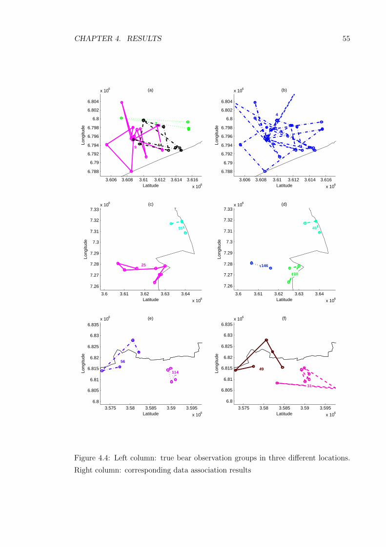
CHAPTER 4. RESULTS 55
3.606 3.608 3.61 3.612 3.614 3.616
x 106
6.788
6.79
6.792
6.794
6.796
6.798
6.8
6.802
6.804
x 106
2
9 44
Latitude
Long
itude
(a)
3.606 3.608 3.61 3.612 3.614 3.616
x 106
6.788
6.79
6.792
6.794
6.796
6.798
6.8
6.802
6.804
x 106
4
Latitude
Long
itude
(b)
3.6 3.61 3.62 3.63 3.64
x 106
7.26
7.27
7.28
7.29
7.3
7.31
7.32
7.33x 10⁶
25
55
Latitude
Long
itude
(c)
3.6 3.61 3.62 3.63 3.64
x 106
7.26
7.27
7.28
7.29
7.3
7.31
7.32
7.33x 10⁶
28
48
146
Latitude
Long
itude
(d)
3.575 3.58 3.585 3.59 3.595
x 106
6.8
6.805
6.81
6.815
6.82
6.825
6.83
6.835x 10⁶
56
114
Latitude
Long
itude
(e)
3.575 3.58 3.585 3.59 3.595
x 106
6.8
6.805
6.81
6.815
6.82
6.825
6.83
6.835x 10⁶
31
49
Latitude
Long
itude
(f)
Figure 4.4: Left column: true bear observation groups in three different locations.
Right column: corresponding data association results

CHAPTER 4. RESULTS 56
Dynamic Model
For the second case, we assume that each target exhibits a random walk. The
estimation was performed multiple times with different values of qx and qy, that is,
process noise variance of 1002 to 25002. The observation noise covariance values
were σx = 0.1 and σy = 0.1 which corresponds to the observation error in the
coordinates. The other parameters in the model were same as given for the static
model. The best estimate of the total number of targets was found with qx =
10502 and qy = 10502 as shown in Figure 4.5(b). The Figure 4.5(c) shows the true
distribution of groups while Figure 4.5(d) shows the estimated group distribution
of the best estimate. The groups in the estimated group distribution mostly have
similar number of observations as compared to the true groups, however, some larger
groups have less observations. The comparison of the groups is shown in Figure 4.6,
it is observed that the overlapping structure in the true groups is captured in the
estimated groups to some extent but there are some incorrect associations as well.
0 200 400 600 800 10000
100
200
300
400
500
Observations
(a)
True number of targets
Estimated number of targets
0 200 400 600 800 10000
50
100
150
200
Observations
(b)
True number of targets
Best Estimate
0 50 100 150 2000
10
20
30
40
50
Groups/Targets
Observ
ations/M
easure
ments
(c)
0 50 100 150 2000
5
10
15
20
25
30
Groups/Targets
Observ
ations/M
easure
ments
(d)
Figure 4.5: (a) Different estimated number of targets in time, (b) Best estimate of
the total number of targets, (c) True Group distribution, (d) Group distribution for
the best estimate of the total number of targets.
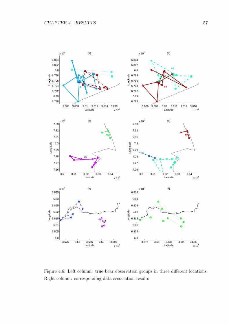
CHAPTER 4. RESULTS 57
3.606 3.608 3.61 3.612 3.614 3.616
x 106
6.788
6.79
6.792
6.794
6.796
6.798
6.8
6.802
6.804
x 106
2
944
Latitude
Long
itude
(a)
3.606 3.608 3.61 3.612 3.614 3.616
x 106
6.788
6.79
6.792
6.794
6.796
6.798
6.8
6.802
6.804
x 106
53
68
Latitude
Long
itude
(b)
3.6 3.61 3.62 3.63 3.64
x 106
7.26
7.27
7.28
7.29
7.3
7.31
7.32
7.33x 10⁶
25
55
Latitude
Long
itude
(c)
3.6 3.61 3.62 3.63 3.64
x 106
7.26
7.27
7.28
7.29
7.3
7.31
7.32
7.33x 10⁶
31
57
87
Latitude
Long
itude
(d)
3.575 3.58 3.585 3.59 3.595
x 106
6.8
6.805
6.81
6.815
6.82
6.825
6.83
6.835x 10⁶
56
114
Latitude
Long
itude
(e)
3.575 3.58 3.585 3.59 3.595
x 106
6.8
6.805
6.81
6.815
6.82
6.825
6.83
6.835x 10⁶
58
Latitude
Long
itude
(f)
Figure 4.6: Left column: true bear observation groups in three different locations.
Right column: corresponding data association results
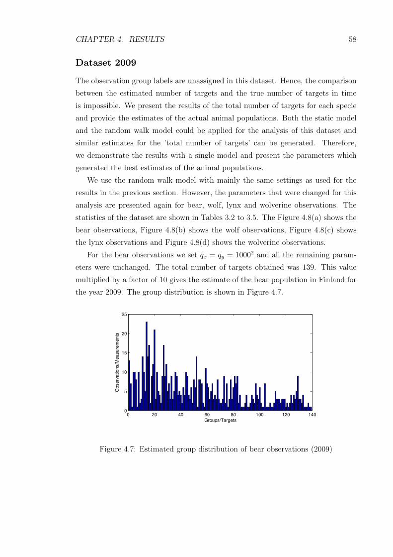
CHAPTER 4. RESULTS 58
Dataset 2009
The observation group labels are unassigned in this dataset. Hence, the comparison
between the estimated number of targets and the true number of targets in time
is impossible. We present the results of the total number of targets for each specie
and provide the estimates of the actual animal populations. Both the static model
and the random walk model could be applied for the analysis of this dataset and
similar estimates for the ’total number of targets’ can be generated. Therefore,
we demonstrate the results with a single model and present the parameters which
generated the best estimates of the animal populations.
We use the random walk model with mainly the same settings as used for the
results in the previous section. However, the parameters that were changed for this
analysis are presented again for bear, wolf, lynx and wolverine observations. The
statistics of the dataset are shown in Tables 3.2 to 3.5. The Figure 4.8(a) shows the
bear observations, Figure 4.8(b) shows the wolf observations, Figure 4.8(c) shows
the lynx observations and Figure 4.8(d) shows the wolverine observations.
For the bear observations we set qx = qy = 10002 and all the remaining param-
eters were unchanged. The total number of targets obtained was 139. This value
multiplied by a factor of 10 gives the estimate of the bear population in Finland for
the year 2009. The group distribution is shown in Figure 4.7.
0 20 40 60 80 100 120 1400
5
10
15
20
25
Groups/Targets
Observ
ation
s/M
easu
rem
ents
Figure 4.7: Estimated group distribution of bear observations (2009)
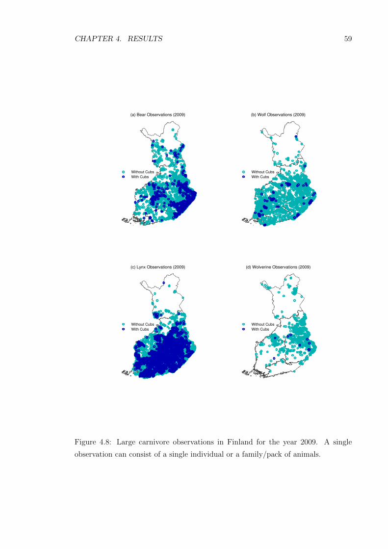
CHAPTER 4. RESULTS 59
(a) Bear Observations (2009)
Without Cubs
With Cubs
(b) Wolf Observations (2009)
Without Cubs
With Cubs
(c) Lynx Observations (2009)
Without Cubs
With Cubs
(d) Wolverine Observations (2009)
Without Cubs
With Cubs
Figure 4.8: Large carnivore observations in Finland for the year 2009. A single
observation can consist of a single individual or a family/pack of animals.
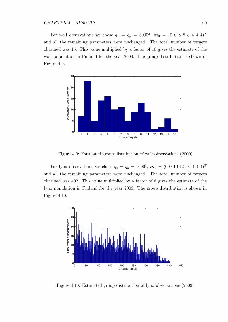
CHAPTER 4. RESULTS 60
For wolf observations we chose qx = qy = 30002, m0 = (0 0 8 8 8 4 4 4)T
and all the remaining parameters were unchanged. The total number of targets
obtained was 15. This value multiplied by a factor of 10 gives the estimate of the
wolf population in Finland for the year 2009. The group distribution is shown in
Figure 4.9.
1 2 3 4 5 6 7 8 9 10 11 12 13 14 150
5
10
15
20
25
Groups/Targets
Ob
serv
ation
s/M
easu
rem
ents
Figure 4.9: Estimated group distribution of wolf observations (2009)
For lynx observations we chose qx = qy = 10002, m0 = (0 0 10 10 10 4 4 4)T
and all the remaining parameters were unchanged. The total number of targets
obtained was 402. This value multiplied by a factor of 6 gives the estimate of the
lynx population in Finland for the year 2009. The group distribution is shown in
Figure 4.10.
0 50 100 150 200 250 300 350 400 4500
5
10
15
20
25
30
Groups/Targets
Observ
ations/M
easure
ments
Figure 4.10: Estimated group distribution of lynx observations (2009)
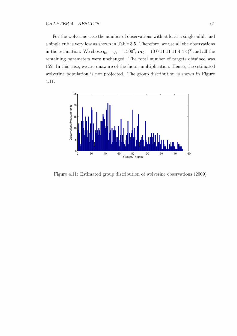
CHAPTER 4. RESULTS 61
For the wolverine case the number of observations with at least a single adult and
a single cub is very low as shown in Table 3.5. Therefore, we use all the observations
in the estimation. We chose qx = qy = 15002, m0 = (0 0 11 11 11 4 4 4)T and all the
remaining parameters were unchanged. The total number of targets obtained was
152. In this case, we are unaware of the factor multiplication. Hence, the estimated
wolverine population is not projected. The group distribution is shown in Figure
4.11.
0 20 40 60 80 100 120 140 1600
5
10
15
20
25
Groups/Targets
Ob
serv
ation
s/M
easu
rem
en
ts
Figure 4.11: Estimated group distribution of wolverine observations (2009)
Chapter 5
Conclusion and Discussion
In this thesis, we have presented a novel approach for the problem of estimating
wild animal population from an unconventional dataset. We incorporated animal
movement models with the state-space modeling framework for estimating the size
of animal populations. We showed the method of formulating the problem as a
conditionally linear Gaussian state-space model and recursively estimating the state
of the animals. We applied the multiple target tracking methodology for tracking
an ‘unknown number of targets’ to the animal observation datasets.
We developed a computational method to solve the problem of estimating large
carnivores in Finland and showed that both static and dynamic models with ap-
propriate parameters generate population estimates that are very close to the ones
generated with the manual analysis on the datasets by the Finnish Game and Fish-
eries Research Institute. The estimation with the static model in particular can be
considered close to the standard animal abundance estimation methodology in the
sense that we assume the animals to be stagnant. On the other hand, the estimation
with the random walk model can be considered more realistic because the animals
move during the time between the observations. However, accurate parameterization
of this model is difficult due to the large area and time frame of the observations.
The models used in this work were mainly parameterized by intuition and such
that the results remain similar to the ones produced by the Finnish Game and
Fisheries Research Institute. However, the parameterization of the models needs to
be automated. More specifically, a statistical parameter estimation method could
be utilized before the application of the Rao-Blackwellized Monte Carlo data as-
sociation algorithm to the animal datasets. The parameters could be estimated
by utilizing individual animal movement datasets, for example, GPS data could be
used. Although, RBMCDA comprises both births and deaths of targets, the as-
62
CHAPTER 5. CONCLUSION AND DISCUSSION 63
sumption of an open population including immigration and emigration could also
be modeled using the population dynamics models. The models used in this work
could be enhanced by incorporating parameters of the habitual and social behav-
ior of the animals. Furthermore, landscape information about the habitats of the
animals could also be utilized.
The group labels that were considered to be true for the results in this thesis are
not exactly correct. Therefore, further improvement in the original manual analysis
is also required. The data based only on sighting information is very unreliable,
hence the method of data collection requires improvement. The foot size width
was the only attribute measurement useful for the data association process in the
RBMCDA, adding more attributes to the state could enhance the accuracy of the
associations. We classified the animals into adult and cubs based on foot size and
seasonal information. This could be improved by including only a single individual
in each observation and providing the exact age of the individual in addition to the
foot size.
Another on going phase in this project is the development of a software tool that
will aid scientists and researchers in computing the size of wild animal populations
automatically. This thesis provides a basis for many new research directions. This
work can be extended for other species datasets as well. The computational method
provides wildlife managers and researchers with a method of efficiently computing
the estimate of an animal population when there are multiple sources of information
in the animal datasets and the number of observations are greater than the actual
number of animals.

Bibliography
Anderson, D. (2001). The need to get the basics right in wildlife field studies.
Wildlife Society Bulletin, 29(4):1294–1297.
Anderson-Sprecher, R. and Ledolter, J. (1991). State-space analysis of wildlife
telemetry data. Journal of the American Statistical Association, 86(415):596–602.
Bar-Shalom, Y. (1987). Tracking and data association. Academic Press Professional,
Inc.
Bar-Shalom, Y. and Li, X. (1995). Multitarget-multisensor tracking: principles and
techniques. Storrs, CT: University of Connecticut, 1995.
Bar-Shalom, Y., Li, X., Li, X., and Kirubarajan, T. (2001). Estimation with appli-
cations to tracking and navigation. Wiley-Interscience.
Blackman, S. and Popoli, R. (1999). Design and analysis of modern tracking systems.
Artech House Norwood, MA.
Borger, L., Dalziel, B., and Fryxell, J. (2008). Are there general mechanisms of
animal home range behaviour? a review and prospects for future research. Ecology
letters, 11(6):637–650.
Breitenmoser, U. (2000). Action plan for the conservation of the Eurasian lynx in
Europe (Lynx lynx). Number 18-112. Council of Europe.
Brillinger, D., Preisler, H., Ager, A., Kie, J., and Stewart, B. (2002). Employing
stochastic differential equations to model wildlife motion. Bulletin of the Brazilian
Mathematical Society, 33(3):385–408.
Buckland, S., Anderson, D., Burnham, K., Laake, J., Borchers, D., and Thomas, L.
(2004a). Advanced distance sampling: estimating abundance of biological popula-
tions. Oxford University Press Oxford, UK.
64
BIBLIOGRAPHY 65
Buckland, S., Goudie, I., and Borchers, D. (2000). Wildlife population assessment:
past developments and future directions. Biometrics, 56(1):1–12.
Buckland, S., Newman, K., Fernandez, C., Thomas, L., and Harwood, J. (2007).
Embedding population dynamics models in inference. Statistical Science, pages
44–58.
Buckland, S., Newman, K., Thomas, L., and Koesters, N. (2004b). State-space
models for the dynamics of wild animal populations. Ecological modelling, 171(1-
2):157–175.
Delahay, R. and Wilson, G. (2001). A review of methods to estimate the abun-
dance of terrestrial carnivores using field signs and observation. Wildlife Research,
28(2):151–164.
Doucet, A., De Freitas, N., and Gordon, N. (2001). Sequential Monte Carlo methods
in practice. Springer Verlag.
Durban, J. and Elston, D. (2005). Mark-recapture with occasion and individual
effects: abundance estimation through bayesian model selection in a fixed di-
mensional parameter space. Journal of agricultural, biological, and environmental
statistics, 10(3):291–305.
Gimenez, O., Bonner, S., King, R., Parker, R., Brooks, S., Jamieson, L., Gros-
bois, V., Morgan, B., and Thomas, L. (2009). Winbugs for population ecologists:
Bayesian modeling using markov chain monte carlo methods. Modeling demo-
graphic processes in marked populations, pages 883–915.
Grewal, M., Andrews, A., and Corporation, E. (2001). Kalman filtering: theory and
practice using MATLAB. Wiley Online Library.
Julier, S. and Uhlmann, J. (2004). Unscented filtering and nonlinear estimation.
Proceedings of the IEEE, 92(3):401–422.
Katajisto, J. (2006). Habitat use and population dynamics of brown bears (Ursus
arctos) in Scandinavia. Doctoral dissertation, University of Helsinki.
Kirubarajan, T. and Bar-Shalom, Y. (2005). Probabilistic data association tech-
niques for target tracking in clutter. Proceedings of the IEEE, 92(3):536–557.
Landa, A., Linden, M., and Kojola, I. (2000). Action plan for the conservation of
wolverines (Gulo gulo) in Europe. Council of Europe Press, Strasbourg.
BIBLIOGRAPHY 66
Leslie, P. (1945). On the use of matrices in certain population mathematics.
Biometrika, 33(3):183–212.
Liukkonen, T., Mykra, S., Bisi, J., and Kurki, S. (2009). Conflicts and compromises
in lynx (lynx lynx) conservation and management in finland. Wildlife Biology,
15(2):165–174.
Madon, B., Gimenez, O., McArdle, B., Scott Baker, C., and Garrigue, C. (2011). A
new method for estimating animal abundance with two sources of data in capture-
recapture studies. Methods in Ecology and Evolution.
Mills, L., Citta, J., Lair, K., Schwartz, M., and Tallmon, D. (2000). Estimating an-
imal abundance using noninvasive dna sampling: promise and pitfalls. Ecological
Applications, 10(1):283–294.
Morales, J., Moorcroft, P., Matthiopoulos, J., Frair, J., Kie, J., Powell, R., Merrill,
E., and Haydon, D. (2010). Building the bridge between animal movement and
population dynamics. Philosophical Transactions of the Royal Society B: Biolog-
ical Sciences, 365(1550):2289.
Newman, K. (1998). State-space modeling of animal movement and mortality with
application to salmon. Biometrics, pages 1290–1314.
Newman, K., Fernandez, C., Thomas, L., and Buckland, S. (2009). Monte carlo in-
ference for state–space models of wild animal populations. Biometrics, 65(2):572–
583.
Nielsen, A., Bigelow, K., Musyl, M., and Sibert, J. (2006). Improving light-
based geolocation by including sea surface temperature. Fisheries Oceanography,
15(4):314–325.
Øksendal, B. (2003). Stochastic differential equations: an introduction with applica-
tions. Springer Verlag.
Patterson, T., Thomas, L., Wilcox, C., Ovaskainen, O., and Matthiopoulos, J.
(2008). State-space models of individual animal movement. Trends in ecology
& evolution, 23(2):87–94.
Pollock, K. (2000). Capture-recapture models. Journal of the American Statistical
Association, 95(449):293–296.
BIBLIOGRAPHY 67
Pollock, K., Nichols, J., Simons, T., Farnsworth, G., Bailey, L., and Sauer, J. (2002).
Large scale wildlife monitoring studies: statistical methods for design and analysis.
Environmetrics, 13(2):105–119.
Preisler, H., Ager, A., Johnson, B., and Kie, J. (2004). Modeling animal movements
using stochastic differential equations. Environmetrics, 15(7):643–657.
Ristic, B., Arulampalam, S., and Gordon, N. (2004). Beyond the Kalman filter:
Particle filters for tracking applications. Artech House Publishers.
Royer, F., Fromentin, J., and Gaspar, P. (2005). A state-space model to derive
bluefin tuna movement and habitat from archival tags. Oikos, 109(3):473–484.
Salvatori, V. and Linnell, J. (2005). Report on the conservation status and threats
for wolf (canis lupus) in europe. Councel of Europe. PVS/Inf (2005), 16.
Sarkka, S. (2006). Recursive Bayesian inference on stochastic differential equations.
Doctoral dissertation, Helsinki University of Technology.
Sarkka, S., Vehtari, A., and Lampinen, J. (2007). Rao-Blackwellized particle filter
for multiple target tracking. Information Fusion, 8(1):2–15.
Schwarz, C. and Seber, G. (1999). Estimating animal abundance: review iii. Statis-
tical Science, pages 427–456.
Seber, G. (1986). A review of estimating animal abundance. Biometrics, pages
267–292.
Smouse, P., Focardi, S., Moorcroft, P., Kie, J., Forester, J., and Morales, J. (2010).
Stochastic modelling of animal movement. Philosophical Transactions of the Royal
Society B: Biological Sciences, 365(1550):2201.
Southwood, R. and Henderson, P. (2000). Ecological methods. Wiley-Blackwell.
Thompson, W., White, G., and Gowan, C. (1998). Monitoring vertebrate popula-
tions. Academic Press San Diego, California, USA.
White, G. (2000). Modeling population dynamics. Ecology and management of mam-
mals in North America. Prentice-Hall, Upper Saddle River, New Jersey, pages
84–107.
Wikman, M. (2010). Monitoring game abundance in Finland in 2010. Riista- ja
kalatalous - Selvityksia. Finnish Game and Fisheries Research Institute.

BIBLIOGRAPHY 68
Witmer, G. (2005). Wildlife population monitoring: some practical considerations.
Wildlife Research, 32(3):259–263.