Statistical Data Processing in Rocket-Space Technology

Modern Applied Science; Vol. 9, No. 8; 2015 ISSN 1913-1844 E-ISSN 1913-1852

Published by Canadian Center of Science and Education

317

Statistical Data Processing in Rocket-Space Technology

Bulat-Batyr Saukhymovich Yesmagambetov1, Zhambyl Talkhauly Ajmenov1, Alexander Mikhailovich Inkov1, Abdushukur Satybaldievich Saribayev1 & Serik Umirbayevich Ismailov1

1 M. Auezov South Kazakhstan State University, Kazakhstan

Correspondence: Bulat-Batyr Saukhymovich Yesmagambetov, M. Auezov South Kazakhstan State University, 160018, Shymkent, Tauke-Khana Street, 5, Kazakhstan. Tel: 7701-460-7116. E-mail: [email protected]

Received: December 3, 2014 Accepted: January 9, 2015 Online Published: July 30, 2015

doi:10.5539/mas.v9n8p317 URL: http://dx.doi.org/10.5539/mas.v9n8p317

Abstract The most measured data in the rocket-and-space technics is a broadband non-stationary random process. Using traditional methods of cyclic digitalization at processing of such data leads to heavy computational costs and heavy amounts of memory of on-board computing devices. As a rule, in processing of discontinuous processes, the recovery of original implementation on the receiving side is not required and processing involves calculation of probabilistic characteristics. In this case processing of data in the rocket-and-space technics has a number of features. First, random processes always represented by the sole implementation. Secondly, priori knowledge of measured random process probabilistic properties is not possible. Thirdly, there is need in on-line processing that predetermines use of rapid processing methods. The article considers application possibilities of nonparametric solution theory methods for evaluation of probabilistic properties of non-stationary broadband random processes in the rocket-and-space technics on-board systems.

Keywords: Rocket-and-space telemetry, random process, data compaction, non-parametric methods, order statistic, stationary hypothesis

1. Introduction 1.1 Introduce the Problem

At the rocket and space technology always has been a pressing problem transferring to Earth in real-time telemetry data rate (Mamchev, 2007). This problem buys a special urgency by transmission to the land of parameters of propulsion systems, such as temperature and combustion chamber pressure, a fuel rate. The knowledge of these parameters in real rate of time allows making operatively a solution at origin of emergencies in propulsion systems.

1.2 Explore Importance of the Problem

Physical parameters in propulsion systems (for example, temperature and combustion-chamber pressure), always look like broad-band no stationary random process with a breadth of a spectrum 2÷32 kilohertz, i.e. represent a non stationary trend from the broad-band random component superimposed on it. However, in the modern rocket-engineering systems for measurement of these parameters often use low-frequency transmitters which on an exit give not the random determined signal (trend) (Voronov, 2011). Thus, the random component of physical process is filtrated. Such mode of measurement and handling of parameters is applied for the purpose of abbreviation of computing costs and decrease of demands to radio engineering communication channels as frequency of an initial cyclical digitization Δt depends on a signal spectrum ΔF (Novikov, 2003). In practice, this relation is equal

1

(5 10)t

FΔ =

÷ Δ

Here (5÷10) means that the coefficient gets out in the range from 5 to 10 depending on the demanded restoration accuracy. From the ratio given above it is visible that measurement and processing of broadband signals requires increase in speed of onboard computing means and their memory sizes in tens times, and at data transmission it is necessary to increase by Earth in ten times the capacity of communication channels. Meanwhile, there is a practical need of reduction of characteristics of onboard computing means that it is connected with requirements of reduction of their mass-dimensional characteristics and energy consumption.

www.ccsenet.org/mas Modern Applied Science Vol. 9, No. 8; 2015

318

Representation of physical parameters in the form of a no stationary low-frequency trend is justified, if space vehicle flight passes in a regular condition. However, the history of assimilation of an outer space knows many facts of accidents of space vehicles. For example, accidents of the American orbiting space crafts of reusable use Space Shuttle, the Russian launchers «Proton» in the end of past century happened because of uninominal situations in propulsion systems. In addition, if in the second case business was limited to loss of satellites, in the first case numerous loss of human life took place. In our opinion, measurement of data on physical parameters in the combustion chamber of motive systems in full, i.e. measurement of a non-stationary broadband signal, and not just trend, has paramount importance. It is connected with that the casual component starts reacting to the coming nearer emergency situation much earlier, than a trend. Thus, the random component is as though a forerunner of an uninominal situation. In addition, its measurement and transmission to the Earth in real rate of time allows making operative solutions on the Earth, in particular to generate a pilot signal on a cut-off of drives and not to suppose accidents.

Thus, the problem of working out of accelerated processing methods of broadband random processes in onboard radio telemetry systems is extremely actual.

Importance of this problem strongly increases if necessary to treat huge data arrays in deadlines.

It gains a special urgency in connection with sharp magnification of a volume of the treated data called by expansion of a scale and research problems, and also rushing to more detailed research of measured processes.

Such demand, naturally, leads to essential thickening as telemetry systems, and radio engineering communication channels.

1.3 Solutions to the Problem

Solution of problems was possible at use of so-called methods of compression data (Ivanov, 2008; Salamon, 2004).

As a rule, in a spectrum of measured parameters the leading position is occupied with broad-band processes (Mala, 2007). Introduction of methods of quasireversible compression of data is effective only for slowly changing processes. Therefore, it does not solve a problem of cumulative reduction of volume of transmitted data and unloading of a communication channel.

Thus, the special urgency is gained by a problem of compression of broad-band signals which make all (10÷30) % from the general nomenclature of measured parameters, but load the transmission channel on (60÷80) %. (Ivanov, 2007; Molodchik, 2002)

For compression of broad-band signals it is possible to use methods of irreversible compression of data which consist in definition on a transmitting leg of is informational-measuring system estimations of probabilistic characteristics of measured random processes and their transmission over communication channels.

Difficulties in realization of methods of irreversible compression are significantly higher, in spite of the fact that their efficiency that is reductions of redundancy of data 10 times more. These results from the fact that the data processed onboard very often represent the only realization of non-stationary casual processes in the absence of aprioristic data on a type of function of distribution. The modern mathematical statistics does not arrange methods for an estimation of probabilistic characteristics of such processes.

2. Method The assessment of probabilistic characteristics of non-stationary casual process is possible the basis on of adaptive division of temporary series of observations into stationarity sites with use of the nonparametric theory of decision-making. (Gamiz, 2011; Gibbons, 2010, Kvam, 2002; Richardson, 2005). Thus, the measured process structure can be described by additive-multiplicative model of the next form (Figure 1):

( ) ( ) ( )y t X t F t= + .

Here y(t) – the measured non-stationary casual process, X(t) – a stationary component of casual process, F(t) – a non-stationary trend.


319

Figure 1. Additive-multiplicative model of the signal

The essence of methods consists in check of a statistical hypothesis of stationarity based on selective data of the measured process with use nonparametric statistics.

In this article the way of division of an interval of supervision into stationarity intervals according to the flowchart provided on figure 2 is offered.

Figure 2. Algorithm of division of an interval of supervision into stationarity intervals

К=1

Insertion of given data

K even-numbered ?

Counter of readings i

Counter of intervals K

Solving scheme

YES

K

YES

YES

NO

NO

NO

NO

NOYES

YES


320

The flowchart in figure 2 is explained in section 2.1.

2.1 Division of an Interval of Observation into Intervals of Stationarity

The algorithm works as follows. Nonparametric statistics, known in literature as Kendal statistics (Tarasenko, 1976; Sheskin, 2003; Sprent, 2001) is formed by ,i ky y sampling data of the measured process.

12

1 1

( , )n n

i ki k i

T u y y−

= = +

= ,

where:

1, ( , )

0, i k

i ki k

y yu y y

y y

≥= ≤

Boundary 2minT and 2

maxT values are at the same time calculated. (Formulas for calculation of 2minT and 2

maxT

aren't given as it is "know-how" of authors of article). Further we can see comparison of 2iT function with 2

maxT

and 2minT , i.e. the statistical hypothesis of stationarity is formed. Casual process with beforehand the set

probability P = 1-α is considered stationary when performing the following condition: 2minT ≤ 2

iT < 2maxT . If P it

is probability of that the hypothesis of stationarity will be true, α is a probability of that the hypothesis of

stationarity will be not true. α is called as a significance value. Calculation of 2iT , 2

minT and 2maxT depends from

α. If 2iT < 2

minT or 2iT ≥ 2

maxT , a site of stationarity is considered certain. After this the ( , )i ku y y sign

function “transfered” into the converse and 2iT , 2

minT and 2maxT clearing into the null state, 2 2 2

max min 0iT T T= = =

(Figure 3). Further, the evaluation process of 2 2 2max min , ,iT T T and comparison procedure is repeated for a new

stationarity interval (Yesmagambetov, 2007; Yesmagambetov, 2006). This means, the dynamic observational

series is divided into any quantity of sections of different length on which a process with specified probability is

considered stationary. The sequence of intervals of stationarity of different duration will be result of application

of the specified procedure. On stationarity intervals average value of casual process with probability Р=1-α is

considered constant.

Figure 3. Separation of the observational data on the stationarity intervals


321

In figure 3 on a horizontal axis are shown number of counting on stationarity intervals. For example, the means that on the 3rd interval of stationarity there is a of counting.

2.2 Nonparametric Estimation of Mean Value Random Process

As known, that there are no universal estimations of probabilistic characteristics for the wide class of random processes (Golovnyh, 2005). For example, maximum likelihood estimates

( 2

1 1

1 1, ( )

N N

o i o i oi i

m x D x mN N= =

= = − )

are optimum for Gaussian distributed random numbers. However, they aren't effective for evenly distributed numbers, and also with correlation between counting of Gaussian casual process. Thus, the a priori knowledge of an aspect of a cumulative distribution function of measured random process is a necessary condition of correct sampling of estimations of statistical performances. It is especially important if to consider that at information handling, as a rule, it is necessary to deal with the only realization of nonstationary casual process. However, in practice a priori informations about measured process are often absent. That practically expels a feasibility of usual parametric modes for statistical handling.

This case, the various algorithms based on adaptation to absolute properties of implementation used: iterated methods of search of quasioptimum conditions of an estimation by volume samples, to length of implementation or a digitization pitch; methods of successive approximations, tests and errors (Karpenko, 2011; 2013).

However, such algorithms are labour-consuming enough and represent too large demands to microcomputer performances. Therefore, response of the microcomputer should make up 62 million simple 60 operations per second at handling of 32 signals with a breadth of a spectrum of 4 kilohertz, and core budget for storage of programs, input data and outcomes of handling should make 2 thousand 8-discharge words.

Thus, procedure of deriving of optimum estimations of probabilistic characteristics is tightly connected with problems of minimization of computing costs. Simplification of estimations of probabilistic characteristics was possibly at use of ordinal statisticians (OS) of ranked a series (RS).

(1) (2) ( ) ( )... ...R Nx x x x≤ ≤ ≤ ≤ ≤

of random numbers gained on the interval of stationarity in sequence. Here (1)x - ordinal statistics of the ranged row on a stationarity interval. Ranging can be made both in ascending order, and in decreasing order.

In a number of studies carried out the errors of estimating the probability characteristics of order statistics. However, these activities were restricted to study of stationary random process while the particular interest represents deriving of estimations of probabilistic characteristics on samples of nonstationary random process.

Application of ordinal statisticians allows to use simple enough procedures for the calculation of average value of casual process, based on central ordinal statistics (COS) ranked beside (Tarasenko, 1975; Daivid, 1979).

( )11 cm x= ;

12 ( 1)cm x

+= ;

21 ( 1) ( )

1( )

2 c cm x x

−= + ;

22 ( ) ( 1)

1( )

2 c cm x x

+= + ;

2 ( ) ( )

1( )

2j c c jm x x

+= + ;

31 ( 1) ( ) ( 1)

1( )

3 c c cm x x x

− += + + .

There are estimates based on the truncation ranked series

( )

2

412

1;

2 i

N

i

m xN

−

=

=−

( )4

1;

i

N j

ji j

m xN j

−

=

=−

And also using extreme ordinal statistics

51 ( ) (1)

1( )

2 Nm x x= + ;

52 ( 1) (2)

1( )

2 Nm x x

−= + ;

( 1) ( )

1( )

2 N j jjm x x− +

= + .


322

The estimations using various combinations of enumerated estimations can be synthesised:

61 ( 1) ( 2)

1( )

2 K Km x x= + ,

where 1 [0.73 ]K E N= , 2 [0.23 ]K E N= ;

62 ( 1) ( 2)

1( ),

2 K Km x x= +

where 1 [0.75 ]K E N= , 2 [0.25 ]K E N= ;

71 1 ( 1)Km xφ= ⋅ ;

72 1 ( 1) 2 ( 2)K Km x xφ φ= ⋅ + ⋅ ;

7 1 ( 1) 2 ( 2) ( )... ,

j K K j Kjm x x x j Nφ φ φ= ⋅ + ⋅ + ⋅ <<

81 12 ( 1) ( 2)( )

K Km x xφ= ⋅ + ;

82 12 ( 1) ( 2) 34 ( 3) ( 4)( ) ( )

K K K Km x x x xφ φ= ⋅ + + ⋅ + ;

8 12 ( 1) ( 2) ( ) ( )( ) ... ( )

j K K ij Ki Kjm x x x xφ φ= ⋅ + + ⋅ + .

where φ – specially chosen multiplier which choice in this article isn't considered.

2.3 Nonparametric Estimation of a Random-Process Variance

When measuring the dispersion is advisable to use the same number of the ranked order statistics as in the estimation of the mean value. At the same time, it is best not to evaluate the dispersion of the process itself, and the ratio of the mean square deviation (MSD). To estimate MSD in nonparametric statistics using the simplest function of scope

( ) (1)1 NW x x= −

and function of "subrange"

( 1) ( )n j jjW x x− +

= − ,

using extreme order statistics ranked series:

( ) (1)11

( 1) ( 2)12

( ),

( )N

N

x x

x x

σ ν

σ ν−

= −

= −

.

It is possible to use estimations also:

3 ( 1) ( 2)( )

j K Kx xσ ν= −

where for σ31 1 [0.75 ]K E N= , 2 [0.25 ]K E N= ;

and for σ32 1 [0.73 ]K E N= 2 [0.25 ]K E N= ;

3 ( 1) ( 2)( )

j K Kx xσ ν= −

5 ( 1)( )

Kxσ ν= ;

52 12 ( 1) ( 2) 34 ( 3) ( 4)( ) ( )

K K K Kv x x v x xσ = + + + ;

5 1 ( 1) 2 ( 2) ( ).. ...j K K j Kj

v x v x v xσ + += + +

As in the case of estimating the average, different combinations of central order statistics and extreme order


323

statistics (EOS):

4 ( ) ( ) )(j c j c j

x xσ ν+ −

= −

2 ( 1) ( 1) )(j N j c j

x xσ ν− + − +

= −

The coefficient ν can be assigned from a wide range; however, the most effective factor values are as follows (Mamchev, 2007):

1;...1 / 2;...1 / 3;...1 / 4;ν =

2.4 Nonparametric Estimation of Function of Distribution of Casual Process

The ranked number of order statistics can be used to estimate the function of distribution of casual process F(x) and function of density f(x). In this case, it suffices to estimate one of them and indirectly to estimate the other, respectively, differentiating F(x) and integrating f(x). With regard to the technique of transmission of telemetry data it is better assess the function of distribution of casual process F(x). This connected with the greater complexity in the implementation of methods for estimating f(x) and better noise immunity transfer F(x) compared to f(x), because of the continuous increase in the ordinate F(x). Therefore, consideration of methods of estimating function of distribution of casual process be paid more attention.

The classic definition of the distribution function, as the probability of the event (x(t) <x) allows us to write the following relation.

0

1( ) Prob( ( ) ) ( ),x

i

NF x x t x c x x

N N= < = = −

Where - Prob(…) means probability, N - sample size, Nx - number of samples of the process x(t), not exceeding the value of x, ( )ic x x− - the comparison function.

1,( )

0,i

ii

x xc x x

x x

≥− = <

Statistical relationship between the sample value and its rank allows us to write the following approximate value:

( )1 1( ) ( )1.R

RF x F x

N= =

+ ,

where R is a rank of counting of X(R) in the ranged row.

Modification of this method, based on fixation as quantile not order statistic x(R) of rank R, but a linear combination Q of order statistics

( )( )1

q

QQR q

q

x A x=

=

allow to generate the following estimates

( 1) ( )

( ) ( 1)

( 1) ( ) ( 1)

2

3

4

1( ( )) ;2 11

( ( )) ;2 11

( ( )) .3 1

R R

R R

R R R

RF x x

NR

F x xN

RF x x x

N

−

+

− +

+ =+

+ =+

+ + =+

At these estimations in the capacity of a quantile magnitude, average of two or three ordinal statisticians is fixed.

Other mode of the estimation of a cumulative distribution function is based on the evaluation of a nonparametric tolerant interval (L2-L1) where L1 and L2 name 100 β - percent independent of distribution F(x) tolerance limits at level γ and

( 2) ( 1)Prob ( )

L LF F β γ − ≥ =


324

If to suppose L1=x(R), and L2=x(S), where R <S the tolerant interval [x(R), x(S)] is equal to the sum of elementary shares from R-th to S-th, i.e.

( ) ( )

11

( )

1

1

!Prob[( ] (1 )

( 1)!( )!

1 ( , 1) ( ) (1 ) .

R S

S R n S Rx x

S Ri N i

i

NF Z Z dz

S R N S R

NI S R N S R

i

β

β

β γ

β β

− − − −−

− −−

=

≥ = = × − =− − − +

= − − − + + = −

Thus γ is a function of arguments N, S-R and β. There are some minimum value Nmin to which in each specific case there matches quite certain combination R and S. It is possible to determine

1( 1)

2N N − tolerant intervals

with various level γ between which N/2 and N (N-1)/2 (depending on that even or odd N) will be symmetric. For security of symmetry of a rank should be connected a condition:

1S N R= − + .

Then for an estimation of cumulative distribution function F5(x) in points x(R) and x(S) with a confidence coefficient γ is possible to accept the following magnitudes:

( )

( )

5

5

1 ( , )( ) ,

21 ( , )

( ) .2

R

S

R SF x

R SF x

β

β

−=

+=

Thus, changing value R from 1 to N/2 and computing matching values S, it is possible to gain estimation F5(x) in N points.

Another mode of nonparametric estimation F6(x) can be generated from definition of a nonparametric confidence interval [ ( )Rx , ( )R Kx + ] for a quantile xp level p. The Confidence level γ is determined from a relation:

6 ( ) 6 ( )Prob(F ( )) ( ) ( , 1) ( , 1)R R K p px p F x I R N K I R K N R Kγ += ≤ ≤ = − + − + − − + ,

where ( , )pI n m – Beta - Prison’s function

1 1( )( , ) (1 ) .

( ) ( )

Pn m

p

O

Г n mI n m x x dx

Г n Г m− −+= −

⋅

In addition, the probability γ that the quantile хр will appear between ordinal statistics ( )Rx and ( )R Kx + does not

depend on an aspect of initial distribution F(x).

3. Results Comparative analysis of the following methods of estimation of the distribution function showed that in terms of the volume of the most satisfactory computational costs are estimates of the form F1, F2, F3 and F4. In addition, F6 is much more complicated than an estimation of aspect F5 in implementation and on their use for this reason is undesirable.

Error analysis of the mean and mean-square deviation values in the random process had been carried out by statistical modeling method in Mathcad environment.

Random function X(t) with distribution function of ( , , )rnorm N μ σ form having Gaussian (normal) distribution with mean μ and mean-square deviation σ (for example μ=1, σ =0) have been used for the modeling.

Signal (trend) F(t) has been stipulated on the random function of the next form

1( ) (1 exp( ))F t A a t= ⋅ − − ,

Where А and 1a are varied in different limits for the modeling aims.

Trend of F(t) = t form has been stipulated in a number of cases.

In a result we have generated the non-stationary random process (Figure 4):


325

( ) ( ) ( )Y t X t F t= +

Figure 4. Generating example of the non-stationary random process

In figure 4 by black color non-stationary casual process y(t), blue color – F(t) trend, red color – 11 ( )cm X=

function is shown.

Valuation of the mean value by 11 ( )cm X= formula allows in point of fact approximate F(t) trend by graduated

multinomial (multinomial of zero power) (Figure 5). On the figure 5 we have four sections of quasi-stationarity

with the length in 9 readings, 35 readings, 57 and 59 readings respectively.

The modeling results showed the following.

Error of the estimated mean essentially depends on the trend form and on the proportion of random and nonrandom components (noise/signal relationship) (Karpenko, 2014; Mala, 2005).

Figure 5. Separation of the non-stationary component (red color non - stationary casual process y(t), blue color –

F(t) trend, black color – 11 ( )cm X= )

The change of the relationship in the stationary component power to the non-stationary component amplitude


326

(noise/signal relationship) leads to the change in the calculation of average value of casual process. Thus, change in the noise/signal relationship within the range from 0.14 to 0.8 leads to the change in the calculation of average value of casual process by 3 times (Figure 6 and Figure 7).

Figure 6. Dependence of an error of calculation of average value on a significance value

The fore cited dependences point on the presence of clear-cut error minimum of the non-stationary estimated mean which is in the range of significance value α = 0.05÷0.06l. Error increase at α value, which are out of this range explained by two properties. On the one hand, there is increase in the stationarity hypothesis region at α < 0.05 value that leads to the decrease in the non-stationary component separation accuracy. On the other hand, there is decrease in the quantity of readings for the stationarity participation at the decrease in the stationarity hypothesis region (α > 0.06) that leads to the increase in the estimated mean error. α=0.05÷0.06 minimum position does not depend on the trend character and the noise/signal relationship.

Figure 7. Dependence of an error of calculation of average value on a significance value

In figures 6 and 7 σ/A - noise/signal relationship, where σ – a mean square deviation of a casual component, A – trend amplitude.

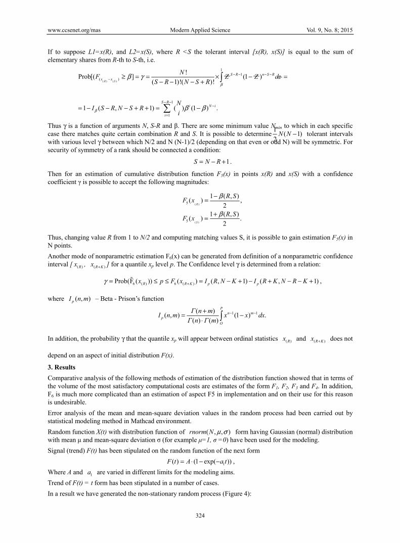
It is obvious that the central order statistics are the easiest to implement. In Figure 8 shows a comparative analysis of different methods of computational cost estimation of the average. The minimum costs, apparently, have estimations of an aspect

11m and

12m .


327

Figure 8. The comparative analysis of computing costs of an estimation

In figure 8 S and T – the memory size and average time of calculation at realization on the microcomputer of the elementary ways of estimation of average value.

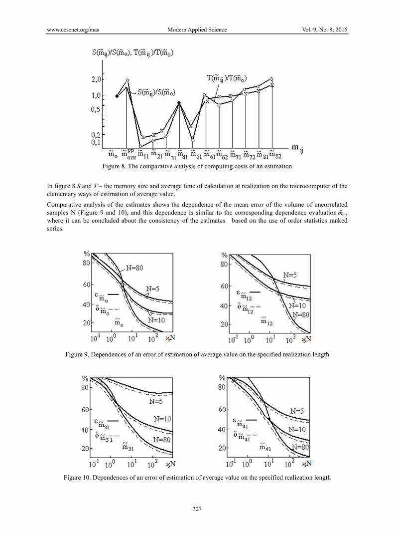
Comparative analysis of the estimates shows the dependence of the mean error of the volume of uncorrelated samples N (Figure 9 and 10), and this dependence is similar to the corresponding dependence evaluation 0m , where it can be concluded about the consistency of the estimates based on the use of order statistics ranked series.

Figure 9. Dependences of an error of estimation of average value on the specified realization length

Figure 10. Dependences of an error of estimation of average value on the specified realization length


328

The following designations are given in figures 9 and 10:

ϗN – the specified realization length, where ϗ= 1/ KN ; KN , - number of counting on a correlation interval; ε, δ – estimation errors.

The considered COS - count the best indicators of accuracy has a simple estimate of the form 12

m , having

besides the minimum computational cost. Uncertainties in estimates using extreme order statistics, for small N is

not worse than the COS - estimates, but for large values of N, they are less effective than simple estimates of the

form 11

m and 12

m . In class evaluations, using truncation ranked series, the quality of estimates increases with

decreasing j. This is especially noticeable in the region of small N. For large values of N (N> 50) decrease j

virtually no effect on the quality of estimates. Estimates of species

6 7 8, ,

j j jm m m ,

No preferential have areas of use in mind more complex computing operations to obtain them. These dependences for all modes of evaluation are at least attributable to the value of N is the sample size equal to 20÷30 counts. These dependencies are common to all types trender. Deterioration of the accuracy for N> 30 is due to non-stationarity of the process being measured, that for large sample sizes to have a greater impact on accuracy than the increase in sample size.

With a sample size of 20-30 counts, errors of all estimates does not exceed 30%.

From these dependences it is possible to conclude that the most effective, both in terms of accuracy of the estimations, and in the sense of minimizing the computational cost is a simple estimate of the form-DSP

12 ( 1)cm x +=

The analysis of the conducted researches at a variance estimation has shown that at the fixed value of factor ν there are no satisfactory estimations in a broad band of modification N. At values N=const the more correlative association between references, the more demanded value of a factor. On Figure 11 values of lapses for different estimations are reduced at various factors ν depending on a sample size for uncorrelated references. From the reduced associations it is visible that value of factor ν is necessary for appointing in the adaptive image, proceeding from a sample size.

Use of estimations of type 2 jσ and 4 jσ is unpromising, as any of these estimations does not give comprehensible accuracy 30%δσ < in all range of modification N at any values of factor ν. Aspect estimations

3 jσ and 5 jσ are less preferable in comparison with the estimations using extreme ordinal statisticians, in view of large computing costs.

Thus, the most comprehensible is estimations of an aspect11

σ and12

σ , yielding satisfactory outcomes in a broad band of modification N. Optimum conditions of an estimation can be noted in a following aspect:

11opt ( ) (1)

1 15,3( ), ,1

154

N

N

x x

N

νσ σ ν

ν

<== = − = ≥

.


329

Figure 11. Dependence of an error of estimation of the mean square deviation of counting on a

stationarity interval

Estimation application11

σ leads to a lost significance in comparison with a maximum likelihood estimate0

σ no

more than 5 %. Almost satisfactory outcomes (δ <30 %) are gained at 5 < N < 40. The decline of estimations at

N> 40 is connected, as well as in case of an average estimation, uncorrelated measured random process.

The study estimates the error 1( )F x shows that the error in the ranked series is always lower than at the

boundaries of the series, where the values 1( )F x associated with rare events. Associations of lapses of an

estimation on a sample size testifies that sample size magnification at a strong correlation between references

does not lead to lapse decrease. Lapse decrease at the fixed sample size was possibly decrease of extent of

correlation between references. In the absence of a correlation improving of quality of an estimation happens to

sample size magnification. Comprehensible outcomes are gained at N> 10. However at N > 40 the decline of

estimations called by agency nonstationarity of process is observed. At uncorrelated references the estimation

1( )F x is worse than the modifications of all on 2..3 % (Figure 12), and at magnification N (N> 80) this

difference in lapses of estimations F1, F2, F3 and F4 practically disappears. Therefore, considering that use of

modified estimations gives an insignificant scoring on accuracy, it is possible to consider optimum more simple

estimation

1( ) .1

RF x

N=

+


330

Figure 12. Dependence of an error of estimation of distribution function on number of counting on a stationarity

interval

Thus, application of the best estimations of an aspect 12

m , 11

σ and 1( )F x allows to use the same ranked a

series of ordinal statisticians for an estimation of such different probabilistic characteristics of random process,

as an average, a variance and a cumulative distribution function. This fact is very important, as it allows first,

substantially reduce the computational cost of the preparation of these estimates, and secondly, allows a single

measurement to obtain almost full information about the measured process. The sample size, as appears from the

analysis of lapses of estimations12

m ,11

σ also 1( )F x should be appointed proceeding from an interval of 15÷30

references. Thus, lapses of estimations do not exceed 20%.

Unfortunately, at such approach it is not possible to gain correlation function estimations as deriving of

estimations12

m ,11

σ and 1( )F x is connected with the demand of statistical independence between references.

4. Discussion Sampling of an optimum pitch of a digitization. In references there are various approaches to sampling of a pitch of a digitization Δt. The majority of recommendations assumes to make a digitization of random process, proceeding from the theorem of Katelnikov. In some activities it is supposed to determine a digitization pitch depending on accuracy of approximation of estimations of correlation function random process. However, too high demands to frequency of inquiry in the first case and a priori independence of a correlation function in the second does not allow to use these techniques at handling of broad-band random process.

In a number of activities it is recommended for the basis at sampling of a pitch of a digitization to accept absolute error of restoration of continuous implementation.

However, it is possible to consider as the most comprehensible criterion assigning of a pitch of a digitization proceeding from a statistical lapse of gained estimations. As analytical research of expressions for lapses is difficult for fulfilling because of bulkiness, the analysis of lapses was made by a modelling method on the computer.

As variances of estimations have a minimum sampling of a quasioptimum pitch of a digitization kt KτΔ = К is possible, ensuring an estimation of probabilistic characteristics with a margin error, close to minimum at possible a smaller amount of references in implementation. In this case kτ - a correlation interval for which at an average estimation to a variance accept a time of the first intersection normalized a level correlation function

0.30λ = . At an estimation of a cumulative distribution function, the sampling step can be appointed by the same technique, as qualitatively character of behaviour of a lapse of an estimation of a cumulative distribution function same, as at average estimations to a variance. Level λ in this case starts equal 0.7. Thus, accuracy of an


331

estimation worsens on 3÷5 %, and the sample size in comparison with an optimum estimation is divided out almost to an order.

However, as value of a correlation function a priori is not known, for a correlation interval kτ it is better to adopt a value an integral interval of correlation

0

( ) ,k dτ ρ τ τ∞

=

Where ( )ρ τ - the normalized correlation function of the random process.

Singularity of application of an integral interval of correlation is that this magnitude connected with an effective breadth of a spectrum efFΔ simple association

1

2k efFτ Δ =

and in this case it is enough for assigning of a pitch of a digitization a priori knowledge only a spectrum breadth.

Outcomes of researches have shown that at an average estimation an effective mode of assigning of a pitch of a digitization is sampling of its condition of independence of selective references as presence of a correlation worsens accuracy of an estimation (Figure 13). Therefore in this case

1.

2kef

tF

τΔ = =Δ

Figure 13. Dependence of an error of calculation of average value on a digitization interval

Agency of a correlation on accuracy is characteristic, though to a less degree, and for a variance and cumulative distribution function estimation (Figure 14 and 15). The conducted researches have shown that the pitch of a digitization for these cases should be appointed from a relation

1 1.

2 4kef

tF

τΔ = =Δ


332

Figure 14. Dependence of an error of calculation of a mean square deviation on a digitization interval

Figure 15. Dependence of an error of function evaluation of distribution on a digitization interval

Necessity of deriving of all estimations of probabilistic characteristics on the same sampled data does not allow gaining an optimality simultaneously for all estimations owing to different demands to a digitization pitch. In this case, as the most important is the information on mean value, it is expedient to choose a digitization pitch

tΔ equal to a correlation interval τк and to gain optimum estimations of a nonstationary average. Variance and cumulative distribution function estimations in this case though will not be optimum will be comprehensible enough.

5. Conclusion Random processes in the rocket-and-space technics, as a rule represented by the sole implementation in conditions of expected uncertainty on the kind of distribution function. Processing of such processes on-line is possible using nonparametric solution theory methods. The present work considers technique for the dynamic observational series division on stationarity intervals with the following valuation of mean values and dispersion.

In the future, we are planning to perform researches on valuation of the distribution function and correlation function of the non-stationary broadband random process.

References Daivid, G. (1979). Ordinal statisticians-М: the Science, 336.

Gamiz, M. L. (2011). Applied Nonparametric Statistics in Reliability. Springer, p. 230. http://dx.doi.org/10.1007/978-0-85729-118-9

Gibbons, J. D. (2010). Subhabrata Chakraborti. Nonparametric Statistical Inference (5th ed.). Chapman and Hall/CRC.

Golovnyh, A. (2003). Digital inhabitancy. CHIP. Computers and communications. K.: The publishing dwelling


333

The Software the Press, 1, 68-70.

Ivanov, V. G., Lomonosov, U. B., & Lyubarsky, M. G. (2008). Analiz and classification of methods of compression of the information/.//Bulletin NTU HPI. Thematic issue: Information science and modelling. Kharkov: NTU KhPI, 49, 78-86.

Ivanov, V. G., Lyubarsky, M. G, & Lomonosov, U. V. (2007). Abbreviation of substantial redundancy of images on the basis of classification of plants and a hum. Control and Information Science Problems, 3, 93-102.

Karpenko, A. P. (2013). Hybrid population algorithms of parametric optimization of design solutions. Information Technology Application, 12, 6-15.

Karpenko, A. P., & Babichenko, A. B. (2014). Nejrosetevoe forecasting of a fuel rate by the aircraft. Aerospace instrument making, 4, 47-56.

Karpenko, A. P., Kulesh, D. S., & Fedin, V. A. (2011). Construction of domain boundary of reachability of dynamic system by a combination of methods multi finish and approximation of a field of vectors. Science and Education: Electronic Scientifically-Engineering Issuing, 5. Retrieved from http://technomag.edu.ru/doc/185335.html

Kvam, P. H., & Vidakovic, B. (2007). Nonparametric Statistics with Applications to Science and Engineering. John Wiley AND Sons, Inc. http://dx.doi.org/10.1002/9780470168707

Mala, S. (2005). Wavelets in handling of signals.-М: Mir, 27-30.

Mamchev, G. V. (2007). The radio communication and television bases. The manual for high schools.-m: the Hot line-a Telecom, 416.

Mionov, S. (2005). Electronic archives for the industry. Open Systems, 2, 56-60.

Molodchik, P. A. (2002). video compression: the present and future//the Computer review. The Publishing Dwelling ІТС, 33, 49-51.

Novikov, S. A. (2005). Video observation Data transfer on IP-webs. Open Systems, 9, 57-59.

Richardson, J. (2005). Video code. Н. 264 and MPEG-4 Standards of new generation. The Technosphere, p. 368.

Salamon, D. (2004). Compression of data, images and a sound. Technosphere, 368.

Sheskin, D. J. (2003). Handbook of Parametric and Nonparametric Statistical Procedures. Chapman AND Hall/CRC, p. 1184. http://dx.doi.org/10.1201/9781420036268

Sprent, P., & Smeeton, N. C. (2001). Applied Nonparametric Statistical Methods. ChapmanandHall/CRC, p. 462.

Tarasenko, F. P. (1976). Nonparametric statistics-Tomsk: Publishing house of Tomsk university, p. 293.

Voronov, Е. М., Karpenko, A. P., & Fedin, V. A. (2011). Parallel construction of assemblage of reachability of the highly-maneuverable aircraft by a "multifinish" method. Bulletin NNSU, 3, 194-200.

Yesmagambetov, B. (2007). Using of not parametrical criteria atirreversible compression of the data. Turk Dunyasi Arastirmalari, 171, 1-6.

Yesmagambetov, B. B. S. (2006). Optimization of parameters of the associative device of compression of data. The bulletin of the Kazakh National Engineering University of K.Satpaev, 3(53), 126-130.

Copyrights Copyright for this article is retained by the author(s), with first publication rights granted to the journal.

This is an open-access article distributed under the terms and conditions of the Creative Commons Attribution license (http://creativecommons.org/licenses/by/3.0/).

Statistical Data Processing in Rocket-Space Technology

Documents

Transcript of Statistical Data Processing in Rocket-Space Technology