Statistical Analysisi Usin STATA

A Handbook of

Statistical Analyses using Stata

Second Edition

c© 2000 by Chapman & Hall/CRC

Sophia Rabe-Hesketh Brian Everitt

CHAPMAN & HALL/CRC

A Handbook of

Statistical Analyses using Stata

Second Edition

Boca Raton London New York Washington, D.C.

This book contains information obtained from authentic and highly regarded sources.Reprinted material is quoted with permission, and sources are indicated. A wide variety ofreferences are listed. Reasonable efforts have been made to publish reliable data and infor-mation, but the author and the publisher cannot assume responsibility for the validity of allmaterials or for the consequences of their use.

Neither this book nor any part may be reproduced or transmitted in any form or by any means,electronic or mechanical, including photocopying, microfilming, and recording, or by anyinformation storage or retrieval system, without prior permission in writing from the publisher.

The consent of CRC Press LLC does not extend to copying for general distribution, forpromotion, for creating new works, or for resale. Specific permission must be obtained inwriting from CRC Press LLC for such copying.

Direct all inquiries to CRC Press LLC, 2000 N.W. Corporate Blvd., Boca Raton, Florida33431.

Trademark Notice:

Product or corporate names may be trademarks or registered trademarks,and are used only for identification and explanation, without intent to infringe.

© 2000 by Chapman & Hall/CRC

No claim to original U.S. Government worksInternational Standard Book Number 1-58488-201-8

Library of Congress Card Number 00-027322Printed in the United States of America 1 2 3 4 5 6 7 8 9 0

Printed on acid-free paper

Library of Congress Cataloging-in-Publication Data

Rabe-Hesketh, S.A handbook of statistical analyses using Stata / Sophia Rabe-Hesketh,

Brian Everitt.—2nd ed.p. cm.

Rev. ed. of: Handbook of statistical analysis using Stata. c1999.Includes bibliographical references and index.ISBN 1-58488-201-8 (alk. paper)1. Stata. 2. Mathematical statistics—Data processing. I. Everitt, Brian. II. Rabe-Hesketh, S. Handbook of statistical analysis using Stata. III. Title.

QA276.4 .R33 2000519,5

′

0285

′5369

—dc21 00-027322 CIP

Preface

Stata is an exciting statistical package which can be used for many standardand non-standard methods of data analysis. Stata is particularly useful formodeling complex data from longitudinal studies or surveys and is thereforeideal for analyzing results from clinical trials or epidemiological studies. Theextensive graphic facilities of the software are also valuable to the modern data-analyst. In addition, Stata provides a powerful programming language thatenables ‘taylor-made’ analyses to be applied relatively simply. As a result, manyStata users are developing (and making available to other users) new programsreflecting recent developments in statistics which are frequently incorporatedinto the Stata package.

This handbook follows the format of its two predecessors, A Handbook ofStatistical Analysis using S-Plus and A Handbook of Statistical Analysis usingSAS. Each chapter deals with the analysis appropriate for a particular set ofdata. A brief account of the statistical background is included in each chapterbut the primary focus is on how to use Stata and how to interpret results. Ourhope is that this approach will provide a useful complement to the excellentbut very extensive Stata manuals.

We would like to acknowledge the usefulness of the Stata Netcourses in thepreparation of this book. We would also like to thank Ken Higbee and MarioCleves at Stata Corporation for helping us to update the first edition of thebook for Stata version 6 and Nick Cox for pointing out errors in the firstedition. This book was typeset using LATEX.

All the datasets can be accessed on the inernet at the following web-sites:• http://www.iop.kcl.ac.uk/IoP/Departments/BioComp/stataBook.stm• http://www.stata.com/bookstore/statanalyses.html

S. Rabe-HeskethB. S. EverittLondon, December 99


http://www.iop.kcl.ac.uk/IoP/Departments/BioComp/stataBook.stm

http://www.stata.com/bookstore/statanalyses.html


To my parents, Brigit and George RabeSophia Rebe-Hesketh

To my wife, Mary ElizabethBrian S, Everitt

Contents

1 A Brief Introduction to Stata1.1 Getting help and information1.2 Running Stata1.3 Datasets in Stata1.4 Stata commands1.5 Data management1.6 Estimation1.7 Graphics1.8 Stata as a calculator1.9 Brief introduction to programming1.10 Keeping Stata up to date1.11 Exercises

2 Data Description and Simple Inference: Female PsychiatricPatients2.1 Description of data2.2 Group comparison and correlations2.3 Analysis using Stata2.4 Exercises

3 Multiple Regression: Determinants of Pollution in U.S. Cities3.1 Description of data3.2 The multiple regression model3.3 Analysis using Stata3.4 Exercises

4 Analysis of Variance I: Treating Hypertension4.1 Description of data4.2 Analysis of variance model4.3 Analysis using Stata4.4 Exercises

5 Analysis of Variance II: Effectiveness of Slimming Clinics5.1 Description of data


5.2 Analysis of variance model5.3 Analysis using Stata5.4 Exercises

6 Logistic Regression: Treatment of Lung Cancer andDiagnosis of Heart Attacks6.1 Description of data6.2 The logistic regression model6.3 Analysis using Stata6.4 Exercises

7 Generalized Linear Models: Australian School Children7.1 Description of data7.2 Generalized linear models7.3 Analysis using Stata7.4 Exercises

8 Analysis of Longitudinal Data I: The Treatment of PostnatalDepression8.1 Description of data8.2 The analysis of longitudinal data8.3 Analysis using Stata8.4 Exercises

9 Analysis of Longitudinal Data II: Epileptic Seizuresand Chemotherapy9.1 Introduction9.2 Possible models9.3 Analysis using Stata9.4 Exercises

10 Some Epidemiology10.1 Description of data10.2 Introduction to Epidemiology10.3 Analysis using Stata10.4 Exercises

11 Survival Analysis: Retention of Heroin Addicts in MethadoneMaintenance Treatment11.1 Description of data11.2 Describing survival times and Cox’s regression model11.3 Analysis using Stata11.4 Exercises


12 Principal Components Analysis: Hearing Measurementusing an Audiometer12.1 Description of data12.2 Principal component analysis12.3 Analysis using Stata12.4 Exercises

13 Maximum Likelihood Estimation: Age of Onset ofSchizophrenia13.1 Description of data13.2 Finite mixture distributions13.3 Analysis using Stata13.4 Exercises

Appendix: Answers to Selected Exercises

References


CHAPTER 1

A Brief Introduction to Stata

1.1 Getting help and information

Stata is a general purpose statistics package which was developed and is main-tained by Stata Corporation. There are several forms of Stata, “IntercooledStata”, its shorter version “Small Stata” and a simpler to use (point and click)student package “StataQuest”. There are versions of each of these packages forWindows (3.1/3.11, 95, 98 and NT), Unix platforms, and the Macintosh. Inthis book we will describe Intercooled Stata for Windows although most fea-tures are shared by the other versions of Stata.

The Stata package is described in seven manuals (Stata Getting Started,Stata User’s Guide, Stata Reference Manuals 1-4 and the Stata GraphicsManual) and in Hamilton (1998). The reference manuals provide extremelydetailed information on each command while the User’s guide describes Statamore generally. Features which are specific to the operating system are de-scribed in the appropriate Getting Started manual, e.g. Getting started withStata for Windows.

Each Stata-command has associated with it a help-file that may be viewedwithin a Stata session using the help facility. If the required command-namefor a particular problem is not known, a list of possible command-names forthat problem may be obtained using search. Both the help-files and manualsrefer to the reference manuals by “[R] command name”, to the User’s Guideby “[U] chapter number and name”, and the graphics manual by “[G] name ofentry”.

The Stata web-page (http://www.stata.com) contains information on theStata mailing list and internet courses and has links to files containing exten-sions and updates of the package (see Section 1.10) as well as a “frequentlyasked questions” (FAQ) list and further information on Stata.

The Stata mailing list, Statalist, simultaneously functions as a technical sup-port service with Stata staff frequently offering very helpful responses to ques-tions. The Statalist messages are archived at:http://www.hsph.harvard.edu/statalist

Internet courses, called netcourses, take place via a temporary mailing listfor course organizers and “attenders”; Each week, the course organizers sendout lecture notes and exercises which the attenders can discuss with each other


http://www.stata.com

http://www.hsph.harvard.edu/statalist

until the organizers send out the answers to the exercises and to the questionsraised by attenders.

1.2 Running Stata

When Stata is started, a screen opens as shown in Figure 1.1 containing fourwindows labeled:

• Stata Command

• Stata Results

• Review

• Variables

Figure 1.1 Stata windows.


A command may be typed in the Stata Command window and executed bypressing the Return (or Enter) key. The command then appears next to a fullstop in the Stata Results window, followed by the output. If the output islonger than the Stata Results window, --more-- appears at the bottom of thescreen. Typing any key scrolls the output forward one screen. The scroll-barmay be used to move up and down previously displayed output. However, onlya certain amount of past output is retained in this window. It is therefore agood idea to open a log-file at the beginning of a stata-session. Press the button

, type a filename into the dialog box and choose Open. If the file-namealready exists, another dialog opens to allow you to decide whether to overwritethe file with new output or whether to append new output to the existing file.The log-file may be viewed during the Stata-session and is automatically savedwhen it is closed. A log-file may also be opend and closed using commands:

log using filename, replacelog close

Stata is ready to accept new commands when the prompt (a period) appearsat the bottom of the screen. If Stata is not ready to receive new commandsbecause it is still running or has not yet displayed all the current output, itmay be interrupted by holding down Ctrl and pressing the Pause/Break key

or by pressing the red Break button .A previous command can be accessed using the PgUp and PgDn keys or

by selecting it from the Review window where all commands from the currentStata session are listed. The command may then be edited if required beforepressing Return to execute the command. In practice, it is useful to build up afile containing the commands necessary to carry out a particular data-analysis.This may be done using Stata’s Do-file Editor. The editor may be opened byclicking . Commands that work when used interactively in the commandwindow can then be copied into the editor. The do-file may be saved and allthe commands contained in it may be executed by clicking in the do-fileeditor or using the command

do dofile

A single dataset may be loaded into Stata. As in other statistical packages,this dataset is generally a matrix where the columns represent variables (withnames and labels) and the rows represent observations. When a dataset isopen, the variable names and variable labels appear in the Variables window.The dataset may be viewed as a spread-sheet by opening the Data Browser

with the button and edited by clicking to open the Data Editor. SeeSection 1.3 for more information on datasets.

Most Stata commands refer to a list of variables, the basic syntax being


command varlist

For example, if the dataset contains variables x y and z, then

list x y

lists the values of x and y. Other components may be added to the command,for example adding if exp after varlist causes the command to process onlythose observations satisfying the logical expression exp. Options are separatedfrom the main command by a comma. The complete command structure andits components are described in Section 1.4.

Help may be obtained by clicking on Help which brings up the dialog boxshown in Figure 1.2. To obtain help on a Stata command, assuming the com-

Figure 1.2 Dialog box for help.

mand name is known, select Stata Command.... To find the appropriateStata command first, select Search.... For example, to find out how to fit aCox regression, we can select Search..., type “survival” and press OK. Thisgives a list of relevant command names or topics for which help-files are avail-able. Each entry in this list includes a green keyword (a hyperlink) that may beselected to view the appropriate help-file. Each help-file contains hyperlinks toother relevant help-files. The search and help-files may also be accessed usingthe commands

search survivalhelp cox

except that the files now appear in the Stata Results window where no hyper-links are available.


The selections News, Official Updates, STB and User-written Pro-grams and Stata Web Site all enable access to relevant information on theWeb providing the computer is connected to the internet (see Section 1.10 onkeeping Stata up-to-date).

Each of the Stata windows may be resized and moved around in the usual

way. The fonts in a window may be changed by clicking on the menu buttonon the top left of that window’s menu bar. All these setting are automaticallysaved when Stata is exited.

Stata may be exited in three ways:

• click into the Close button at the top right hand corner of the Statascreen

• select the File menu from the menu bar and select Exit• type exit, clear in the Stata Commands window and press Return.

1.3 Datasets in Stata

1.3.1 Data input and output

Stata has its own data format with default extension .dta. Reading and savinga Stata file are straightforward. If the filename is bank.dta, the commands are

use banksave bank

If the data are not stored in the current directory, then the complete path mustbe specified, as in the command

use c:\user\data\bankHowever, the least error prone way of keeping all the files for a particularproject in one directory is to change to that directory and save and read allfiles without their pathname:

cd c:\user\datause banksave bank

When reading a file into Stata, all data already in memory need to be cleared,either by running clear before the use command or by using the option clearas follows:

use bank, clear

If we wish to save data under an existing filename, this results in an errormessage unless we use the option replace as follows:


save bank, replace

If the data are not available in Stata format, they may be converted to Stataformat using another package (e.g. Stat/Transfer) or saved as an ASCII file(although the latter option means loosing all the labels). When saving data asASCII, missing values should be replaced by some numerical code.

There are three commands available for reading different types of ASCIIdata: insheet is for files containing one observation (on all variables) per linewith variables separated by tabs or commas, where the first line may containthe variable names; infile with varlist (free format) allows line breaks to occuranywhere and variables to be separated by spaces as well as commas or tabs;and infile with a dictionary (fixed format) is the most flexible command.Data may be saved as ASCII using outfile or outsheet.

Only one dataset may be loaded at any given time but a dataset may bemerged with the currently loaded dataset using the command merge or appendto add observations or variables.

1.3.2 Variables

There are essentially two types of variables in Stata, string and numeric. Eachvariable can be one of a number of storage types that require different numbersof bytes. The storage types are byte, int, long, float, and double for numericvariables and str1 to str80 for string variables of different lengths. Besidesthe storage type, variables have associated with them a name, a label, and aformat. The name of a variable y can be changed to x using

rename y x

The variable label can be defined using

label variable x "cost in pounds"

and the format of a numeric variable can be set to “general numeric” with twodecimal places using

format x %7.2g

Numeric variables

Missing values in numeric variables are represented by dots only and are in-terpreted as very large numbers (which can lead to mistakes). Missing valuecodes may be converted to missing values using the command mvdecode. Forexample,

mvdecode x, mv(-99)


replaces all values of variable x equal to −99 by dots and

mvencode x, mv(-99)

changes the missing values back to −99.Numeric variables can be used to represent categorical or continuous vari-

ables including dates. For categorical variables it is not always easy to remem-ber which numerical code represents which category. Value labels can thereforebe defined as follows:

label define s 1 married 2 divorced 3 widowed 4 singlelabel values marital s

The categories can also be recoded, for example

recode marital 2/3=2 4=3

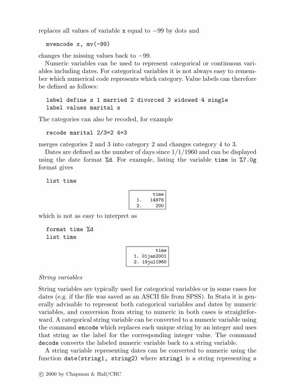
merges categories 2 and 3 into category 2 and changes category 4 to 3.Dates are defined as the number of days since 1/1/1960 and can be displayed

using the date format %d. For example, listing the variable time in %7.0gformat gives

list time

time1. 149762. 200

which is not as easy to interpret as

format time %dlist time

time1. 01jan20012. 19jul1960

String variables

String variables are typically used for categorical variables or in some cases fordates (e.g. if the file was saved as an ASCII file from SPSS). In Stata it is gen-erally advisable to represent both categorical variables and dates by numericvariables, and conversion from string to numeric in both cases is straightfor-ward. A categorical string variable can be converted to a numeric variable usingthe command encode which replaces each unique string by an integer and usesthat string as the label for the corresponding integer value. The commanddecode converts the labeled numeric variable back to a string variable.

A string variable representing dates can be converted to numeric using thefunction date(string1, string2) where string1 is a string representing a


date and string2 is a permutation of "dmy" to specify the order of the day,month and year in string1. For example, the commands

display date("30/1/1930","dmy")

and

display date("january 1, 1930", "mdy")

both return the negative value -10957 because the date is 10957 days before1/1/1960.

1.4 Stata commands

Typing help language gives the following generic command structure for mostStata commands.

[by varlist:] command [varlist] [=exp] [if exp] [in range] [weight][using filename] [, options]

The help-file contains links to information on each of the components, and wewill briefly describe them here:

[by varlist:] instructs Stata to repeat the command for each combina-tion of values in the list of variables varlist.

[command] is the name of the command and can be abbreviated; for exam-ple, the command display can be abbreviated as dis.

[varlist] is the list of variables to which the command applies.[=exp] is an expression.[if exp] restricts the command to that subset of the observations that

satisfies the logical expression exp.[in range] restricts the command to those observations whose indices lie

in a particular range.[weight] allows weights to be associated with observations (see Section 1.6).[using filename] specifies the filename to be used.[options] are specific to the command and may be abbreviated.For any given command, some of these components may not be available,

for example list does not allow [using filename]. The help-files for specificcommands specify which components are available, using the same notationas above, with square brackets enclosing components that are optional. Forexample, help log gives

log using filename [, noproc append replace ]

implying that [by varlist:] is not allowed and that using filename is re-quired whereas the three options noproc, append or replace are optional.

The syntax for varlist, exp and range is described in the next three sub-sections, followed by information on how to loop through sets of variables orobservations.


1.4.1 Varlist

The simplest form of varlist is a list of variable names separated by spaces.Variable names may also be abbreviated as long as this is unambiguous, i.e. x1may be referred to by x only if there is no other variable starting on x such asx itself or x2. A set of adjacent variables such as m1, m2 and x may be referredto as m1-x. All variables starting on the same set of letters can be representedby that set of letters followed by a wild card *, so that m* may stand for m1 m6mother. The set of all variables is referred to by all. Examples of a varlistare

x yx1-x16a1-a3 my* sex age

1.4.2 Expressions

There are logical, algebraic and string expressions in Stata. Logical expressionsevaluate to 1 (true) or 0 (false) and use the operators < and <= for “less than”and “less than or equal to” respectively and similarly > and >= are used for“greater than” and “greater than or equal to”. The symbols == and ~= standfor “equal to” and “not equal to”, and the characters ~, & and | represent“not”, “and” and “ or” respectively, so that

if (y~=2&z>x)|x==1

means “if y is not equal to two and z is greater than x or if x equals one”. Infact, expressions involving variables are evaluated for each observation so thatthe expression really means

(yi �= 2&zi > xi)|xi == 1

where i is the observation index.Algebraic expressions use the usual operators + - * / and ^ for addition,

subtraction, multiplication, division, and powers respectively. Stata also hasmany mathematical functions such as sqrt(), exp(), log(), etc. and statisti-cal functions such as chiprob() and normprob() for cumulative distributionfunctions and invnorm(), etc. for inverse cumulative distribution functions.Pseudo-random numbers may be generated using uniform(). Examples of al-gebraic expressions are

y + x(y + x)^3 + a/binvnorm(uniform())+2

where invnorm(uniform()) returns a (different) sample from the standardnormal distribution for each observation.


Finally, string expressions mainly use special string functions such assubstr(str,n1,n2) to extract a substring starting at n1 for a length of n2.The logical operators == and ~= are also allowed with string variables and theoperator + concatinates two strings. For example, the combined logical andstring expression

("moon"+substr("sunlight",4,5))=="moonlight"

returns the value 1 for “true”.For a list of all functions, use help functions.

1.4.3 Observation indices and ranges

Each observation has associated with it an index. For example, the value ofthe third observation on a particular variable x may be referred to as x[3].The macro n takes on the value of the running index and N is equal to thenumber of observations. We can therefore refer to the previous observation ofa variable as x[ n-1].

An indexed variable is only allowed on the right hand side of an assignment.If we wish to replace x[3] by 2, we can do this using the syntax

replace x=2 if n==3

We can refer to a range of observations using either if with a logical expressioninvolving n or, more easily by using in range, where range is a range ofindices specified using the syntax f/l (for “first to last”) where f and/or lmay be replaced by numerical values if required, so that 5/12 means “fifth totwelfth” and f/10 means “first to tenth” etc. Negative numbers are used tocount from the end, for example

list x in -10/l

lists the last 10 observations.

1.4.4 Looping through variables or observations

Explicitly looping through observations is often not necessary because expres-sions involving variables are automatically evaluated for each observation. Itmay however be required to repeat a command for subsets of observations andthis is what by varlist: is for. Before using by varlist:, however, the datamust be sorted using

sort varlist

where varlist includes the variables to be used for by varlist:. Note that ifvarlist contains more than one variable, ties in the earlier variables are sortedaccording to the next variable. For example,


sort school classby school class: summ test

give the summary statistics of test for each class. If class is labeled from 1to ni for the ith school, then not using school in the above commands wouldresult in the observations for all classes labeled 1 to be grouped together.

A very useful feature of by varlist: is that it causes the observation indexn to count from 1 within each of the groups defined by the unique combinationsof the values of varlist. The macro N represents the number of observations ineach group. For example,

sort group ageby group: list age if n== N

lists age for the last observation in each group where the last observation inthis case is the observation with the highest age within its group.

We can also loop through a set variables or observations using for. Forexample,

for var v*: list X

loops through the list of all variables starting on v and applies the commandlist to each member X of the variable list. Numeric lists may also be used.The command

for num 1 3 5: list vX

lists v1, v3 and v5. Numeric lists may be abbreviated by “first(increment)last”,giving the syntax 1(2)5 for the list 1 3 5 (not an abbreviation in this case!).The for command can be made to loop through several lists (of the samelength) simultaneously where the “current” members of the different lists arereferred to by X, Y, Z, A, B etc. For example, if there are variables v1, v2, v3,v4, and v5 in the dataset,

for var v1-v5 \num 1/5: replace X=0 in Y

replaces the ith value of the variable vi by 0, i.e., it sets vi[i] to 0. Here, wehave used the syntax “first/last” which is used when the increment is 1. Seehelp for for more information, for example on how to construct nested loops.

Another method for looping is the while command which is described inSection 1.9 on programming but may also be used interactively.


1.5 Data management

1.5.1 Generating variables

New variables may be generated using the commands generate or egen. Thecommand generate simply equates a new variable to an expression which isevaluated for each observation. For example,

generate x=1

creates a new variable called x and sets it equal to one. When generate isused together with if exp or in range, the remaining observations are set tomissing. For example,

generate percent = 100*(old - new)/old if old>0

generates the variable percent and set it equal to the percentage decrease fromold to new where old is positive and equal to missing otherwise. The functionreplace works in the same way as generate except that it allows an existingvariable to be changed. For example,

replace percent = 0 if old<=0

changes the missing values in percent to zeros. The two commands abovecould be replaced by the single command

generate percent=cond(old>0, 100*(old-new)/old, 0)

where cond() evaluates to the second argument if the first argument is trueand to the third argument otherwise.

The function egen provides an extension to generate. One advantage ofegen is that some of its functions accept a variable list as an argument, whereasthe functions for generate can only take simple expressions as arguments. forexample, we can form the average of 100 variables m1 to m100 using

egen average=rmean(m1-m100)

where missing values are ignored. Other functions for egen operate on groupsof observations. For example, if we have the income (variable income) formembers within families (variable family), we may want to compute the totalincome of each member’s family using

egen faminc = sum(income), by(family)

An existing variable can be replaced using egen functions only by first droppingit using

drop x

Another way of dropping variables is using keep varlist where varlist isthe list of all variables not to be dropped.


1.5.2 Changing the shape of the data

It is frequently necessary to change the shape of data, the most common ap-plication being grouped data, in particular repeated measures. If we havemeasurement occasions j for subjects i, this may be viewed as a multivari-ate dataset in which each occasion j is represented by a variable xj and thesubject identifier is in the variable subj. However, for some statistical analyseswe may need one single, long, response vector containing the responses for alloccasions for all subjects, as well as two variables subj and occ to representthe indices i and j, respectively. The two “data shapes” are called wide andlong, respectively. We can convert from the wide shape with variables xj andsubj given by

list

x1 x2 subj1. 2 3 12. 4 5 2

to the long shape with variables x, occ and subj using the syntax

reshape long x, i(subj) j(occ)list

subj occ x1. 1 1 22. 1 2 33. 2 1 44. 2 2 5

and back again using

reshape wide x, i(subj) j(occ)

For data in the long shape, it may be required to collapse the data so that eachgroup is represented by a single summary measure. For example, for the dataabove, each subject’s responses can be summarized using the mean, meanx,and standard deviation, sdx and the number of nonmissing responses, num.This may be achieved using

collapse (mean) meanx=x (sd) sdx=x (count) num=x, by(subj)list

subj meanx sdx num1. 1 2.5 .7071068 22. 2 4.5 .7071068 2

Since it is not possible to convert back to the original format, the data maybe preserved before running collapse and restored again later using the com-mands preserve and restore.


Other ways of changing the shape of data include dropping observationsusing

drop in 1/10

to drop the first 10 observations or

sort group weightby group: keep if n==1

to drop all but the lightest member of each group. Sometimes it may be neces-sary to transpose the data, converting variables to observations and vice versa.This may be done and undone using xpose.

If each observation represents a number of units (as after collapse), it maysometimes be required to replicate each observation by the number of units,num, that it represents. This may be done using

expand num

If there are two datasets, subj.dta, containing subject specific variables, andocc.dta, containing occasion specific variables for the same subjects, then ifboth files contain the same sorted subject identifier subj id and subj.dta iscurrently loaded, the files may be merged as follows:

merge subj id using occ

resulting in the variables from subj.dta being expanded as in the expand com-mand above and the variables from occ.dta being added.

1.6 Estimation

All estimation commands in Stata, for example regress, logistic, poisson,and glm, follow the same syntax and share many of the same options.

The estimation commands also produce essentially the same output and savethe same kind of information. The stored information may be processed usingthe same set of post-estimation commands.

The basic command structure is

[xi:] command depvar [model] [weights], options

which may be combined with by varlist:, if exp and in range. The re-sponse variable is specified by depvar and the explanatory variables by model.The latter is usually just a list of explanatory variables. If categorical explana-tory variables and interactions are required, using xi: at the beginning of thecommand enables special notation for model to be used. For example,

xi: regress resp i.x


creates dummy variables for each value of x except the first and includes thesedummy variables as regressors in the model.

xi: regress resp i.x*y z

fits a regression model with the main effects of x, y, and z and the interactionx×y where x is treated as categorical and y and z as continuous (see help xifor further details).

The syntax for the [weights] option is

weighttype=varname

where weighttype depends on the purpose of weighting the data. If the dataare in the form of a table where each observation represents a group containinga total of freq observations, using [fweight=freq] is equivalent to runningthe same estimation command on the expanded dataset where each observationhas been replicated freq times. If the observations have different standard de-viations, for example, because they represent averages of different numbers ofobservations, then aweights is used with weights proportional to the recipro-cals of the standard deviations. Finally, pweights is used for inverse probabilityweighting in surveys where the weights are equal to the inverse probability thateach observation was sampled. (Another type of weights, iweight, is availablefor some estimation commands mainly for use by programmers).

All the results of an estimation command are stored and can be processedusing post-estimation commands. For example, predict may be used to com-pute predicted values or different types of residuals for the observations in thepresent dataset and the commands test, testparm and lrtest can be usedto carry out various tests on the regression coefficients.

The saved results can also be accesssed directly using the appropriate names.For example, the regression coefficients are stored in global macros calledb[varname]. In order to display the regression coefficient of x, simply type

display b[x]

To access the entire parameter vector, use e(b). Many other results may beaccessed using the e(name) syntax. See the “Saved Results” section of theentry for the estimation command in the Stata Reference Manuals to find outunder what names particular results are stored.

1.7 Graphics

There is a command, graph, which may be used to plot a large number ofdifferent graphs. The graphs appear in a Stata Graph window which is createdwhen the first graph is plotted. The basic syntax is graph varlist, optionswhere options are used to specify the type of graph. For example,


graph x, box

gives a boxplot of x and

graph y x, twoway

gives a scatter-plot with y on the y-axis and x on the x-axis. (The optiontwoway is not needed here because it is the default.) More than the minimumnumber of variables may be given. For example,

graph x y, box

gives two boxplots within one set of axes and

graph y z x, twoway

gives a scatterplot of y and z against x with different symbols for y and z. Theoption by(group) may be used to plot graphs separately for each group. Withthe option box, this results in several boxplots within one set of axes; with theoption twoway, this results in several scatterplots in the same graphics windowand using the same axis ranges.

If the variables have labels, then these are used as titles or axis labels asappropriate. The graph command can be extended to specify axis-labeling, orto specify which symbols should be used to represent the points and how (orwhether) the points are to be connected, etc. For example, in the command

graph y z x, s(io) c(l.) xlabel ylabel t1("scatter plot")

the symbol() option s(io) causes the points in y to be invisible (i) andthose in z to be represented by small circles (o). The connect() option c(l.),causes the points in y to be connected by straight lines and those in z to beunconnected. Finally, the xlabel amd ylabel options cause the x- and y-axesto be labeled using round values (without these options, only the minimumand maximum values are labeled) and the title option t1("scatter plot")causes a main title to be added at the top of the graph (b1(), l1(), r1()would produce main titles on bottom, left and right and t2(), b2(), l2(),r2() would produce secondary titles on each of the four sides).

The entire graph must be produced in a single command. This means, forexample, that if different symbols are to be used for different groups on a scat-tergraph, then each group must be represented by a separate variable havingnonmissing values only for observations belonging to that group. For example,the commands

gen y1=y if group==1gen y2=y if group==2graph y1 y2 x, s(dp)


produce a scatter-plot where y is represented by diamonds (d) in group 1 andby plus (p) in group 2. See help graph for a list of all plotting symbols, etc.Note that there is a very convenient alternative method of generating y1 andy2. Simpley use the command

separate y, by(group)

1.8 Stata as a calculator

Stata can be used as a simple calculator using the command display followedby an expression, e.g.,

display sqrt(5*(11-3^2))

3.1622777

There are also a number of statistical functions that can be used withoutreference to any variables. These commands end in i, where i stands for im-mediate command. For example, we can calculate the sample size required foran independent samples t-test to achieve 80% power to detect a significancedifference at the 1% level of significance (2-sided) if the means differ by onestandard deviation using sampsi as follows:

sampsi 1 2, sd(1) power(.8) alpha(0.01)

Estimated sample size for two-sample comparison of means

Test Ho: m1 = m2, where m1 is the mean in population 1and m2 is the mean in population 2

Assumptions:

alpha = 0.0100 (two-sided)power = 0.8000

m1 = 1m2 = 2

sd1 = 1sd2 = 1

n2/n1 = 1.00

Estimated required sample sizes:

n1 = 24n2 = 24

Similarly ttesti can be used to carry out a t-test if the means, standarddeviations and sample sizes are given.

Results can be saved in local macros using the syntax

local a=exp


The result may then be used again by enclosing the macro name in singlequotes `´ (using two separate keys on the keyboard). For example,

local a=5display sqrt(`a´)

2.236068

Matrices can also be defined and matrix algebra carried out interactively.The following matrix commands define a matrix a, display it, give itstrace and its eigenvalues:

matrix a=(1,2\2,4)matrix list a

symmetric a[2,2]c1 c2

r1 1r2 2 4

dis trace(a)

5

matrix symeigen x v = amatrix list v

v[1,2]e1 e2

r1 5 0

1.9 Brief introduction to programming

So far we have described commands as if they would be run interactively.However, in practice, it is always useful to be able to repeat the entire analysisusing a single command. This is important, for example, when a data entryerror is detected after most of the analysis has already been carried out! InStata, a set of commands stored as a do-file, called, for example, analysis.do,can be executed using the command

do analysis


We strongly recommend that readers create do-files for any work in Stata, i.e.,for the exercises of this book.

One way of generating a do-file is to carry out the analysis interactively andsave the commands, for example, by selecting Save Review Contents fromthe menu of the Review window. Stata’s Do-file Editor can also be used tocreate a do-file. One way of trying out commands interactively and buildingup a do-file is to run commands in the Commands window and copy theminto the Do-file Editor after checking that they work. Another possibility isto type commands into the Do-file Editor and try them out individually byhighlighting the command and clicking into Tools - Do Selection. Alterna-tively, any text-editor or word-processor may be used to create a do-file. Thefollowing is a useful template for a do-file:

/* comment describing what the file does */version 6.0capture log closelog using filename, replaceset more off

command 1command 2etc.

log closeexit

We will explain each line in turn.

1. The “brackets” /* and */ cause Stata to ignore everything between them.Another way of commenting out lines of text is to start the lines with asimple *.

2. The command version 6.0 causes Stata to interpret all commands as ifwe were running Stata version 6.0 even if, in the future, we have actuallyinstalled a later version in which some of these commands do not workanymore.

3. The capture prefix causes the do-file to continue running even if the com-mand results in an error. The capture log close command therefore closesthe current log-file if one is open or returns an error message. (Another usefulprefix is quietly which suppresses all output, except error messages).

4. The command log using filename, replace opens a log-file, replacingany log-file of the same name if it already exists.

5. The command set more off causes all the output to scroll past automat-ically instead of waiting for the user to scroll through it manually. This isuseful if the user intends to look at the log-file for the output.


6. After the analysis is complete, the log-file is closed using log close.

7. The last statement, exit, is not necessary at the end of a do-file but maybe used to make Stata stop runnning the do-file wherever it is placed.Variables, global macros, local macros, and matrices can be used for storing

and referring to data and these are made use of extensively in programs. Forexample, we may wish to subtract the mean of x from x. Interactively, wewould use

summarize x

to find out what the mean value is and then subtract that value from x. How-ever, we should not type the value of the mean into a do-file because the resultwould no longer be valid if the data change. Instead, we can access the meancomputed by summarize using r(mean):

quietly summarize xgen xnew=x-r(mean)

Most Stata commands are r class, meaning that they store result that may beaccessed using r() with the appropriate name inside the brackets. Estimationcommands store the results in e(). In order to find out under what namesconstants are stored, see the “Stored Results” section for the command ofinterest in the Stata Reference Manuals.

If a local macro is defined without using the = sign, anything can appearon the right hand side and typing the local macro name in single quotes hasthe same effect as typing whatever appeared on the right hand side in thedefinition of the macro. For example, if we have a variable y, we can use thecommands

local a ydisp "`a´[1] = " `a´[1]

y[1] = 4.6169958

Local macros are only ‘visible’ within the do-file or program in which theyare defined. Global macros may be defined using

global a=1

and accessed by prefixing them with a dollar, for example,

gen b=$a

Sometimes it is useful to have a general set of commands (or a program) thatmay be applied in different situations. It is then essential that variable namesand parameters specific to the application can be passed to the program. Ifthe commands are stored in a do-file, the ‘arguments’ with wich the do-file


will be used, are referred to as `1´, `2´ etc inside the do-file. For example, ado-file containing the command

list `1´ `2´

may be run using

do filename x1 x2

to cause x1 and x2 to be listed. Alternatively, we can define a program whichcan be called without using the do command in much the same way as Stata’sown commands. This is done by enclosing the set of commands by

program define prognameend

After running the program definition, we can run the program by typing theprogram name and arguments.

A frequently used programming tool both for use in do-files and in programdefinitions is while. For example, below we define a program called mylistthat lists the first three observations of each variable in a variable list:

program define mylistwhile "`1´"~=""{ /* outer loop: loop through variables */

local x `1´local i=1display "`x´"while ì´ <=3 /* inner loop: loop through observations */

display `x´[ì´]local i=ì´+1 /* next observation */

}mac shift /* next variable */display " "

end

We can run the program using the command

mylist x y z

The inner loop simply displays the ì´th element of the variable `x´ for ì´from 1 to 3. The outer loop uses the macro `1´ as follows: At the beginning,the macros `1´, `2´ and `3´ contain the arguments x, y and z respectively,with which mylist was called. The command

mac shift


shifts the contents of `2´ into `1´ and those of `3´ into `2´, etc. Therefore,the outer loop steps through variables x, y and z.

A program may be defined by typing it into the Commands window. Thisis almost never done in practice, however, a more useful method being to definethe program within a do-file where it can easily be edited. Note that oncethe program has been loaded into memory (by running the program definecommands), it has to be cleared from memory using program drop before itcan be redefined. It is therefore useful to have the command

capture program drop mylist

in the do-file before the program define command, where capture ensuresthat the do-file continues running even if mylist does not yet exist.

A program may also be saved in a separate file (containing only the programdefinition) of the same name as the program itself and having the extension.ado. If the ado-file (automatic do-file) is in a directory in which Stata looksfor ado-files, for example the current directory, it can be executed simply bytyping the name of the file. There is no need to load the program first (byrunning the program definition). To find out where Stata looks for ado-files,type

adopath

This lists various directories including \ado\personal/, the directory wherepresonal ado-files may be stored. Many of Stata’s own commands are actuallyado-files stored in the ado subdirectory of the directory where wstata.exe islocated.

1.10 Keeping Stata up to date

Stata Corporation continually updates the current version of Stata. If the com-puter is connected to the internet, Stata can be updated by issuing the com-mand

update all

Ado-files are then downloaded and stored in the correct directory. If the exe-cutable has changed since the last update, a file wstata.bin is also downloaded.This file should be used to overwrite wstata.exe after saving the latter un-der a new name, e.g. wstata.old. The command help whatsnew lists all thechanges since the release of the present version of Stata. In addition to Stata’sofficial updates to the package, new user-written functions are available everytwo months. Descriptions of these functions are published in the Stata Tech-nical Bulletin (STB) and the functions themselves may be downloaded fromthe web. One way of finding out about the latest programs submitted to the


STB is to subscribe to the journal which is inexpensive. Another way is viathe search command. For example, running

search meta

gives a long list of entries including one on STB-42STB-42 sbe16.1 . . . . . New syntax and output for the meta-analysis command

(help meta if installed) . . . . . . . . . . . S. Sharp and J. Sterne3/98 STB Reprints Vol 7, pages 106--108

which reveals that STB-42 has a directory in it called sbe16.1 containing filesfor “New syntax and output for the meta-analysis command” and that help onthe new command may be found using help meta, but only after the programhas been installed.

An easy way of downloading this program is to click on Help - STB &User-written Programs, select http://www.stata.com, click on stb, thenstb42, sbe16 1 and finally, click on (click here to install).

The program can also be installed using the commands

net from http://www.stata.comnet cd stbnet cd stb42net install sbe16_1

Not all user-defined programs are included in any STB (yet). Other ado-filesmay be found on the Statalist archive under “Contributed ADO Files” (directaddress http://ideas.uqam.ca/ideas/data/bocbocode.html).

1.11 Exercises

1. Use an editor (e.g. Notepad, PFE or a word-processor) to generate thedataset test.dat given below, where the columns are separated by tabs (makesure to save it as a text only, or ASCII, file).

v1 v2 v31 3 52 16 35 12 2

2. Read the data into Stata using insheet (see help insheet).

3. Click into the Data Editor and type in the variable sex with values 1 2 and1.

4. Define value labels for sex (1=male, 2=female).

5. Use gen to generate id, a subject index (from 1 to 3).

6. Use rename to rename the variables v1 to v3 to time1 to time3. Aso trydoing this in a single command using for.




http://www.ideas.uqam.ca/ideas/data/bocbocode.html

7. Use reshape to convert the dataset to long shape.8. Generate a variable d that is equal to the squared difference between the

variable time at each occasion and the average of time for each subject.9. Drop the observation corresponding to the third occasion for id=2.


CHAPTER 2

Data Description and Simple Inference:Female Psychiatric Patients

2.1 Description of data

The data to be used in this chapter consist of observations on 8 variables for118 female psychiatric patients and are available in Hand et al. (1994). Thevariables are as follows:• age: age in years• IQ: intelligence questionnaire score• anxiety: anxiety (1=none, 2=mild, 3=moderate, 4=severe)• depress: depression (1=none, 2=mild, 3=moderate, 4=severe)• sleep: can you sleep normally? (1=yes, 2=no)• sex: have you lost interest in sex? (1=no, 2=yes)• life: have you thought recently about ending your life? (1=no, 2=yes)• weight: weight change over last six months (in lb)The data are given in Table 2.1 with missing values coded as -99. One questionof interest is how the women who have recently thought about ending their livesdiffer from those who have not. Also of interest are the correlations betweenanxiety and depression and between weight change, age, and IQ.

Table 2.1: Data in fem.dat

id age IQ anx depress sleep sex life weight

1 39 94 2 2 2 2 2 4.92 41 89 2 2 2 2 2 2.23 42 83 3 3 3 2 2 4.04 30 99 2 2 2 2 2 -2.65 35 94 2 1 1 2 1 -0.36 44 90 -99 1 2 1 1 0.97 31 94 2 2 -99 2 2 -1.58 39 87 3 2 2 2 1 3.59 35 -99 3 2 2 2 2 -1.2

10 33 92 2 2 2 2 2 0.811 38 92 2 1 1 1 1 -1.912 31 94 2 2 2 -99 1 5.5


Table 2.1: Data in fem.dat (continued)

13 40 91 3 2 2 2 1 2.714 44 86 2 2 2 2 2 4.415 43 90 3 2 2 2 2 3.216 32 -99 1 1 1 2 1 -1.517 32 91 1 2 2 -99 1 -1.918 43 82 4 3 2 2 2 8.319 46 86 3 2 2 2 2 3.620 30 88 2 2 2 2 1 1.421 34 97 3 3 -99 2 2 -99.022 37 96 3 2 2 2 1 -99.023 35 95 2 1 2 2 1 -1.024 45 87 2 2 2 2 2 6.525 35 103 2 2 2 2 1 -2.126 31 -99 2 2 2 2 1 -0.427 32 91 2 2 2 2 1 -1.928 44 87 2 2 2 2 2 3.729 40 91 3 3 2 2 2 4.530 42 89 3 3 2 2 2 4.231 36 92 3 -99 2 2 2 -99.032 42 84 3 3 2 2 2 1.733 46 94 2 -99 2 2 2 4.834 41 92 2 1 2 2 1 1.735 30 96 -99 2 2 2 2 -3.036 39 96 2 2 2 1 1 0.837 40 86 2 3 2 2 2 1.538 42 92 3 2 2 2 1 1.339 35 102 2 2 2 2 2 3.040 31 82 2 2 2 2 1 1.041 33 92 3 3 2 2 2 1.542 43 90 -99 -99 2 2 2 3.443 37 92 2 1 1 1 1 -99.044 32 88 4 2 2 2 1 -99.045 34 98 2 2 2 2 -99 0.646 34 93 3 2 2 2 2 0.647 42 90 2 1 1 2 1 3.348 41 91 2 1 1 1 1 4.849 31 -99 3 1 2 2 1 -2.250 32 92 3 2 2 2 2 1.051 29 92 2 2 2 1 2 -1.252 41 91 2 2 2 2 2 4.053 39 91 2 2 2 2 2 5.954 41 86 2 1 1 2 1 0.255 34 95 2 1 1 2 1 3.556 39 91 1 1 2 1 1 2.957 35 96 3 2 2 1 1 -0.6



58 31 100 2 2 2 2 2 -0.659 32 99 4 3 2 2 2 -2.560 41 89 2 1 2 1 1 3.261 41 89 3 2 2 2 2 2.162 44 98 3 2 2 2 2 3.863 35 98 2 2 2 2 1 -2.464 41 103 2 2 2 2 2 -0.865 41 91 3 1 2 2 1 5.866 42 91 4 3 -99 -99 2 2.567 33 94 2 2 2 2 1 -1.868 41 91 2 1 2 2 1 4.369 43 85 2 2 2 1 1 -99.070 37 92 1 1 2 2 1 1.071 36 96 3 3 2 2 2 3.572 44 90 2 -99 2 2 2 3.373 42 87 2 2 2 1 2 -0.774 31 95 2 3 2 2 2 -1.675 29 95 3 3 2 2 2 -0.276 32 87 1 1 2 2 1 -3.777 35 95 2 2 2 2 2 3.878 42 88 1 1 1 2 1 -1.079 32 94 2 2 2 2 1 4.780 39 -99 3 2 2 2 2 -4.981 34 -99 3 -99 2 2 1 -99.082 34 87 3 3 2 2 1 2.283 42 92 1 1 2 1 1 5.084 43 86 2 3 2 2 2 0.485 31 93 -99 2 2 2 2 -4.286 31 92 2 2 2 2 1 -1.187 36 106 2 2 2 1 2 -1.088 37 93 2 2 2 2 2 4.289 43 95 2 2 2 2 1 2.490 32 95 3 2 2 2 2 4.991 32 92 -99 -99 -99 2 2 3.092 32 98 2 2 2 2 2 -0.393 43 92 2 2 2 2 2 1.294 41 88 2 2 2 2 1 2.695 43 85 1 1 2 2 1 1.996 39 92 2 2 2 2 1 3.597 41 84 2 2 2 2 2 -0.698 41 92 2 1 2 2 1 1.499 32 91 2 2 2 2 2 5.7

100 44 86 3 2 2 2 2 4.6101 42 92 3 2 2 2 1 -99.0102 39 89 2 2 2 2 1 2.0



103 45 -99 2 2 2 2 2 0.6104 39 96 3 -99 2 2 2 -99.0105 31 97 2 -99 -99 -99 2 2.8106 34 92 3 2 2 2 2 -2.1107 41 92 2 2 2 2 2 -2.5108 33 98 3 2 2 2 2 2.5109 34 91 2 1 1 2 1 5.7110 42 91 3 3 2 2 2 2.4111 40 89 3 1 1 1 1 1.5112 35 94 3 3 2 2 2 1.7113 41 90 3 2 2 2 2 2.5114 32 96 2 1 1 2 1 -99.0115 39 87 2 2 2 1 2 -99.0116 41 86 3 2 1 1 2 -1.0117 33 89 1 1 1 1 1 6.5118 42 -99 3 2 2 2 2 4.9

2.2 Group comparison and correlations

We have interval scale variables (weight change, age, and IQ), ordinal vari-ables (anxiety and depression), and categorical, dichotomous variables (sexand sleep) that we wish to compare between two groups of women: those whohave thought about ending their lives and those who have not.

For interval scale variables, the most common statistical test is the t-testwhich assumes that the observations in the two groups are independent andare sampled from two populations each having a normal distribution and equalvariances. A nonparametric alternative (which does not rely on the latter twoassumptions) is the Mann-Whitney U-test.

For ordinal variables, either the Mann-Whitney U-test or a χ2-test may beappropriate depending on the number of levels of the ordinal variable. Thelatter test can also be used to compare dichotomous variables between thegroups.

Continuous variables can be correlated using the Pearson correlation. If weare interested in the question whether the correlations differ significantly fromzero, then a hypothesis test is available that assumes bivariate normality. Asignificance test not making this distributional assumption is also available; it isbased on the correlation of the ranked variables, the Spearman rank correlation.Finally, if variables have only few categories, Kendall’s tau-b provides a usefulmeasure of correlation (see, e.g., Sprent, 1993).


2.3 Analysis using Stata

Assuming the data have been saved from a spread-sheet or statistical package(for example SPSS) as a tab-delimited ASCII file, fem.dat, they can be readusing the instruction

insheet using fem.dat, clear

There are missing values which have been coded as -99. We replace these withStata’s missing value code ‘.’ using

mvdecode all, mv(-99)

The variable sleep has been entered incorrectly for subject 3. Such dataentry errors can be detected using the command

codebook

which displays information on all variables; the output for sleep is shownbelow:sleep ------------------------------------------------------------------- SLEEP

type: numeric (byte)

range: [1,3] units: 1unique values: 3 coded missing: 5 / 118

tabulation: Freq. Value14 198 21 3

Alternatively, we can detect errors using the assert command. For sleep,we would type

assert sleep==1|sleep==2|sleep==.

1 contradiction out of 118assertion is false

Since we do not know what the correct code for sleep should have been, wecan replace the incorrect value of 3 by ‘missing’

replace sleep=. if sleep==3

In order to have consistent coding for “yes” and “no”, we recode the variablesleep

recode sleep 1=2 2=1

and to avoid confusion in the future, we label the values as follows:


label define yn 1 no 2 yeslabel values sex ynlabel values life ynlabel values sleep yn

The last three commands could also have been carried out in a for loop

for var sex life sleep: label values X yn

First, we can compare the groups who have and have not thought aboutending their lives by tabulating summary statistics of various variables for thetwo groups. For example, for IQ, we type

table life, contents(mean iq sd iq)

----------+-----------------------LIFE | mean(iq) sd(iq)

----------+-----------------------no | 91.27084 3.757204

yes | 92.09836 5.0223----------+-----------------------

To assess whether the groups appear to differ in their weight loss over thepast six months and to informally check assumptions for an independent sam-ples t-test, we plot the variable weight as a boxplot for each group after defin-ing appropriate labels:

label variable weight "weight change in last six months"sort lifegraph weight, box by(life) ylabel yline(0) gap(5) /*

*/ b2("have you recently thought about ending your life?")

giving the graph shown in Figure 2.1. The yline(0) option has placed a hor-izontal line at 0. (Note that in the instructions above, the “brackets” for com-ments, /* and */ were used to make Stata ignore the line breaks in the middleof the graph command in a d-file). The groups do not seem to differ much intheir median weight change and the assumptions for the t-test seem reasonablebecause the distributions are symmetric with similar spread.

We can also check the assumption of normality more formally by plotting anormal quantile plot of suitably defined residuals. Here the difference betweenthe observed weight changes and the group-specific mean weight changes canbe used. If the normality assumption is satisfied, the quantiles of the residualsshould be linearly related to the quantiles of the normal distribution. Theresiduals can be computed and plotted using

egen res=mean(weight), by(life)replace res=weight-reslabel variable res "residuals of t-test for weight"qnorm res, gap(5) xlab ylab t1("normal q-q plot")


Figure 2.1 Box-plot of weight by group.

where gap(5) was used to reduce the gap between the vertical axis and theaxis title (the default gap is 8). The points in the Q-Q plot in Figure 2.2 aresufficiently close to the staight line.

We could also test whether the variances differ significantly using

sdtest weight, by(life)

giving the output shown in Display 2.1. which shows that there is no signif-icant difference (p=0.57) between the variances. Note that the test for equalvariances is only appropriate if the variable may be assumed to be normallydistributed in each population. Having checked the assumptions, we carry outa t-test for weight change:

ttest weight, by(life)

Display 2.2 shows that the two-tailed significance is p=0.55 and the 95% con-fidence interval for the mean difference in weight change between those whohave thought about ending their lives and those who have not is from -0.74pounds to 1.39 pounds. Therefore, there is no evidence that the populationsdiffer in their mean weight change, but we also cannot rule out a difference inmean weight change of as much as 1.4 pounds in 6 months.


Figure 2.2 Normal Q-Q plot of residuals of weight change.

Variance ratio test

------------------------------------------------------------------------------Group | Obs Mean Std. Err. Std. Dev. [95% Conf. Interval]

---------+--------------------------------------------------------------------no | 45 1.408889 .3889616 2.609234 .6249883 2.19279

yes | 61 1.731148 .3617847 2.825629 1.00747 2.454825---------+--------------------------------------------------------------------combined | 106 1.59434 .2649478 2.727805 1.068997 2.119682------------------------------------------------------------------------------

Ho: sd(no) = sd(yes)

F(44,60) observed = F_obs = 0.853F(44,60) lower tail = F_L = F_obs = 0.853F(44,60) upper tail = F_U = 1/F_obs = 1.173

Ha: sd(no) < sd(yes) Ha: sd(no) ~= sd(yes) Ha: sd(no) > sd(yes)P < F_obs = 0.2919 P < F_L + P > F_U = 0.5724 P > F_obs = 0.7081

Display 2.1


Two-sample t test with equal variances


---------+--------------------------------------------------------------------no | 45 1.408889 .3889616 2.609234 .6249883 2.19279

yes | 61 1.731148 .3617847 2.825629 1.00747 2.454825---------+--------------------------------------------------------------------combined | 106 1.59434 .2649478 2.727805 1.068997 2.119682---------+--------------------------------------------------------------------

diff | -.3222587 .5376805 -1.388499 .743982------------------------------------------------------------------------------Degrees of freedom: 104

Ho: mean(no) - mean(yes) = diff = 0

Ha: diff < 0 Ha: diff ~= 0 Ha: diff > 0t = -0.5993 t = -0.5993 t = -0.5993

P < t = 0.2751 P > |t| = 0.5502 P > t = 0.7249

Display 2.2

We can use a χ2- test to test for differences in depression between the twogroups and display the corresponding cross-tabulation together with the per-centage of women in each category of depression by group using the singlecommand

tabulate life depress, row chi2

| DEPRESSLIFE | 1 2 3 | Total

-----------+---------------------------------+----------no | 26 24 1 | 51

| 50.98 47.06 1.96 | 100.00-----------+---------------------------------+----------

yes | 0 42 16 | 58| 0.00 72.41 27.59 | 100.00

-----------+---------------------------------+----------Total | 26 66 17 | 109

| 23.85 60.55 15.60 | 100.00

Pearson chi2(2) = 43.8758 Pr = 0.000

There is a significant association between depress and life with none of thesubjects who have thought about ending their lives having zero depressioncompared with 51% of those who have not. Note that this test does not takeaccount of the ordinal nature of depression and is therefore likely to be lesssensitive than, for example, ordinal regression (see Chapter 6). Fisher’s exacttest can be obtained without having to reproduce the table as follows:

tabulate life depress, exact nofreq

Fisher’s exact = 0.000


Similarly, for sex, we can obtain the table and both the χ2-test and Fisher’sexact tests using

tabulate life sex, row chi2 exact

| SEXLIFE | no yes | Total

-----------+----------------------+----------no | 12 38 | 50

| 24.00 76.00 | 100.00-----------+----------------------+----------

yes | 5 58 | 63| 7.94 92.06 | 100.00

-----------+----------------------+----------Total | 17 96 | 113

| 15.04 84.96 | 100.00

Pearson chi2(1) = 5.6279 Pr = 0.018Fisher’s exact = 0.032

1-sided Fisher’s exact = 0.017

Therefore, those who have thought about ending their lives are more likely tohave lost interest in sex than those who have not (92% compared with 76%).We can explore correlations between the three variables weight, IQ and ageusing a single command

corr weight iq age

(obs=100)

| weight iq age--------+---------------------------

weight| 1.0000iq| -0.2920 1.0000

age| 0.4131 -0.4363 1.0000

The correlation matrix has been evaluated for those 100 observations that hadcomplete data on all three variables. The command pwcorr may be used toinclude, for each correlation, all observations that have complete data for thecorresponding pair of variables, resulting in different sample sizes for differentcorrelations. The sample sizes and p-values can be displayed simultaneously asfollows:

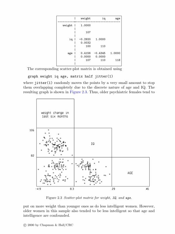
pwcorr weight iq age, obs sig


| weight iq age----------+---------------------------

weight | 1.0000|| 107|

iq | -0.2920 1.0000| 0.0032| 100 110|

age | 0.4156 -0.4345 1.0000| 0.0000 0.0000| 107 110 118|

The corresponding scatter-plot matrix is obtained using

graph weight iq age, matrix half jitter(1)

where jitter(1) randomly moves the points by a very small amount to stopthem overlapping completely due to the discrete nature of age and IQ. Theresulting graph is shown in Figure 2.3. Thus, older psychiatric females tend to

Figure 2.3 Scatter-plot matrix for weight, IQ, and age.

put on more weight than younger ones as do less intelligent women. However,older women in this sample also tended to be less intelligent so that age andintelligence are confounded.


It would be interesting to see whether those who have thought about endingtheir lives have the same relationship between age and weight change as dothose who have not. In order to form a single scatter-plot with different sym-bols representing the two groups, we must use a single variable for the x-axis(age) and plot two separate variables wgt1 and wgt2 which contain the weightchanges for groups 1 and 2, respectively:

gen wgt1 = weight if life==2gen wgt2 = weight if life==1label variable wgt1 "no"label variable wgt2 "yes"graph wgt1 wgt2 age, s(dp) xlabel ylabel /*

*/ l1("weight change in last 6 months") /*

The resulting graph in Figure 2.4 shows that within both groups, higher ageis associated with larger weight increases and the groups do not form distinctclusters.

Figure 2.4 Scatter-plot of weight against age.

Finally, an appropriate correlation between depression and anxiety is Kendall’stau-b which can be obtained using

ktau depress anxiety


Number of obs = 107Kendall’s tau-a = 0.2827Kendall’s tau-b = 0.4951Kendall’s score = 1603

SE of score = 288.279 (corrected for ties)

Test of Ho: depress and anxiety independentPr > |z| = 0.0000 (continuity corrected)

giving a value of 0.50 with an approximate p-value of p < 0.001.

2.4 Exercises

1. Tabulate the mean weight change by level of depression.2. Using for, tabulate the means and standard deviations by life for each of

the variables age, iq and weight.3. Use search nonparametric or search mann or search whitney to find

help on how to run the Mann-Whitney U-test.4. Compare the weight changes between the two groups using the Mann Whit-

ney U-test.5. Form a scatter-plot for IQ and age using different symbols for the two groups

(life=1 and life=2). Explore the use of the option jitter(#) for differentintegers # to stop symbols overlapping.

6. Having tried out all these commands interactively, create a do-file containingthese commands and run the do-file. In the graph commands, use the optionsaving(filename,replace) to save the graphs in the current directory andview the graphs later using the command graph using filename.

See also Exercises in Chapter 6.


CHAPTER 3

Multiple Regression: Determinants ofPollution in U.S. Cities


Data on air pollution in 41 U.S. cities were collected by Sokal and Rohlf (1981)from several U.S. government publications and are reproduced here in Ta-ble 3.1. (The data are also available in Hand et al. (1994).) There is a singledependent variable, so2, the annual mean concentration of sulphur dioxide,in micrograms per cubic meter. These data generally relate to means for thethree years 1969 to 1971. The values of six explanatory variables, two of whichconcern human ecology and four climate, are also recorded; details are as fol-lows:

• temp: average annual temperature in ◦F

• manuf: number of manufacturing enterprises employing 20 or more workers

• pop: population size (1970 census) in thousands

• wind: average annual wind speed in miles per hour

• precip: average annual precipitation in inches

• days: average number of days with precipitation per year.

The main question of interest about this data is how the pollution level asmeasured by sulphur dioxide concentration is determined by the six explana-tory variables. The central method of analysis will be multiple regression.

3.2 The multiple regression model

The multiple regression model has the general form

yi = β0 + β1x1i + β2x2i + · · · + βpxpi + εi (3.1)

where y is a continuous response variable, x1, x2, · · · , xp are a set of explanatoryvariables and ε is a residual term. The regression coefficients, β0, β1, · · · , βp

are generally estimated by least squares. Significance tests for the regressioncoefficients can be derived by assuming that the residual terms are normallydistributed with zero mean and constant variance σ2.

For n observations of the response and explanatory variables, the regression


Table 3.1: Data in usair.dat

Town SO2 temp manuf pop wind precip days

Phoenix 10 70.3 213 582 6.0 7.05 36Little Rock 13 61.0 91 132 8.2 48.52 100San Francisco 12 56.7 453 716 8.7 20.66 67Denver 17 51.9 454 515 9.0 12.95 86Hartford 56 49.1 412 158 9.0 43.37 127Wilmington 36 54.0 80 80 9.0 40.25 114Washington 29 57.3 434 757 9.3 38.89 111Jackson 14 68.4 136 529 8.8 54.47 116Miami 10 75.5 207 335 9.0 59.80 128Atlanta 24 61.5 368 497 9.1 48.34 115Chicago 110 50.6 3344 3369 10.4 34.44 122Indiana 28 52.3 361 746 9.7 38.74 121Des Moines 17 49.0 104 201 11.2 30.85 103Wichita 8 56.6 125 277 12.7 30.58 82Louisvlle 30 55.6 291 593 8.3 43.11 123New Orleans 9 68.3 204 361 8.4 56.77 113Baltimore 47 55.0 625 905 9.6 41.31 111Detroit 35 49.9 1064 1513 10.1 30.96 129Minnisota 29 43.5 699 744 10.6 25.94 137Kansas 14 54.5 381 507 10.0 37.00 99St. Louis 56 55.9 775 622 9.5 35.89 105Omaha 14 51.5 181 347 10.9 30.18 98Albuquerque 11 56.8 46 244 8.9 7.77 58Albany 46 47.6 44 116 8.8 33.36 135Buffalo 11 47.1 391 463 12.4 36.11 166Cincinnati 23 54.0 462 453 7.1 39.04 132Cleveland 65 49.7 1007 751 10.9 34.99 155Columbia 26 51.5 266 540 8.6 37.01 134Philadelphia 69 54.6 1692 1950 9.6 39.93 115Pittsburgh 61 50.4 347 520 9.4 36.22 147Providence 94 50.0 343 179 10.6 42.75 125Memphis 10 61.6 337 624 9.2 49.10 105Nashville 18 59.4 275 448 7.9 46.00 119Dallas 9 66.2 641 844 10.9 35.94 78Houston 10 68.9 721 1233 10.8 48.19 103Salt Lake City 28 51.0 137 176 8.7 15.17 89Norfolk 31 59.3 96 308 10.6 44.68 116Richmond 26 57.8 197 299 7.6 42.59 115Seattle 29 51.1 379 531 9.4 38.79 164Charleston 31 55.2 35 71 6.5 40.75 148Milwaukee 16 45.7 569 717 11.8 29.07 123


model may be written concisely as

y = Xβ + ε (3.2)

where y is the n× 1 vector of responses, X is an n× (p+ 1) matrix of knownconstants, the first column containing a series of ones corresponding to the termβ0 in (3.1) and the remaining columns values of the explanatory variables. Theelements of the vector β are the regression coefficients β0, · · · , βp, and those ofthe vector ε, the residual terms ε1, · · · , εn. For full details of multiple regressionsee, for example, Rawlings (1988).


Assuming the data are available as an ASCII file usair.dat in the currentdirectory and that the file contains city names as given in Table 3.1, they maybe read in for analysis using the following instruction:

infile str10 town so2 temp manuf pop /**/ wind precip days using usair.dat

Before undertaking a formal regression analysis of these data, it will behelpful to examine them graphically using a scatter-plot matrix. Such a dis-play is useful in assessing the general relationships between the variables, inidentifying possible outliers, and in highlighting potential collinearity problemsamongst the explanatory variables. The basic plot can be obtained using

graph so2 temp manuf pop wind precip days, matrix

The resulting diagram is shown in Figure 3.1. Several of the scatter-plots showevidence of outliers and the relationship between manuf and pop is very strongsuggesting that using both as explanatory variables in a regression analysis maylead to problems (see later). The relationships of particular interest, namelythose between so2 and the explanatory variables (the relevant scatterplots arethose in the first row of Figure 3.1) indicate some possible nonlinearity. Amore informative, although slightly more ‘messy’ diagram can be obtained ifthe plotted points are labeled with the associated town name. The necessaryStata instruction is

graph so2-days, matrix symbol([town]) tr(3) ps(150)

The symbol() option labels the points with the names in the town variable; if,however, the full name is used, the diagram would be very difficult to read.Consequently the trim() option, abbreviated tr(), is used to select the firstthree characters of each name for plotting and the psize() option, abbreviatedps(), is used to increase the size of these characters to 150% compared with theusual 100% size. The resulting diagram appears in Figure 3.2. Clearly, Chicagoand to a lesser extent Philadelphia might be considered outliers. Chicago has


Figure 3.1 Scatter-plot matrix.

such a high degree of pollution compared to the other cities that it shouldperhaps be considered as a special case and excluded from further analysis. Anew data file with Chicago removed can be generated using

clearinfile str10 town so2 temp manuf pop wind /*

*/ precip days using usair.dat if town~="Chicago"

or by dropping the opservation using

drop if town=="Chicago"

The command regress may be used to fit a basic multiple regression model.The necessary Stata instruction to regress sulphur dioxide concentration on thesix explanatory variables is

regress so2 temp manuf pop wind precip days

or, alternatively,

regress so2 temp-days

(see Display 3.1)


Figure 3.2 Scatter-plot matrix with town labels.


Source | SS df MS Number of obs = 40---------+------------------------------ F( 6, 33) = 6.20

Model | 8203.60523 6 1367.26754 Prob > F = 0.0002Residual | 7282.29477 33 220.675599 R-squared = 0.5297---------+------------------------------ Adj R-squared = 0.4442

Total | 15485.90 39 397.074359 Root MSE = 14.855

------------------------------------------------------------------------------so2 | Coef. Std. Err. t P>|t| [95% Conf. Interval]

---------+--------------------------------------------------------------------temp | -1.268452 .6305259 -2.012 0.052 -2.551266 .0143631

manuf | .0654927 .0181777 3.603 0.001 .0285098 .1024756pop | -.039431 .0155342 -2.538 0.016 -.0710357 -.0078264

wind | -3.198267 1.859713 -1.720 0.095 -6.981881 .5853469precip | .5136846 .3687273 1.393 0.173 -.2364966 1.263866

days | -.0532051 .1653576 -0.322 0.750 -.3896277 .2832175_cons | 111.8709 48.07439 2.327 0.026 14.06278 209.679

------------------------------------------------------------------------------

Display 3.1

The main features of interest are the analysis of variance table and theparameter estimates. In the former, the ratio of the model mean square to theresidual mean square gives an F-test for the hypothesis that all the regressioncoefficients in the fitted model are zero. The resulting F-statistic with 6 and 33degrees of freedom takes the value 6.20 and is shown on the right hand side;the associated P-value is very small. Consequently the hypothesis is rejected.The square of the multiple correlation coefficient (R2) is 0.53 showing that53% of the variance of sulphur dioxide concentration is accounted for by thesix explanatory variables of interest. The adjusted R2 statistic is an estimateof the population R2 taking account of the fact that the parameters wereestimated from the data. The statistic is calculated as

adj R2 = 1 − (n− i)(1 −R2)n− p

(3.3)

where n is the number of observations used in fitting the model, and i is anindicator variable that takes the value 1 if the model includes an intercept and 0otherwise. The root MSE is simply the square root of the residual mean squarein the analysis of variance table, which itself is an estimate of the parameter σ2.The estimated regression coefficients give the estimated change in the responsevariable produced by a unit change in the corresponding explanatory variablewith the remaining explanatory variables held constant.

One concern generated by the initial graphical material on this data was thestrong relationship between the two explanatory variables manuf and pop. Thecorrelation of these two variables is obtained by using

correlate manuf pop


(obs=40)

| manuf pop--------+------------------

manuf| 1.0000pop| 0.8906 1.0000

The strong linear dependence might be a source of collinearity problems andcan be investigated further by calculating what are known as variance inflationfactors for each of the explanatory variables. These are given by

VIF(xi) =1

1 −R2i

(3.4)

where VIF(xi) is the variance inflation factor for explanatory variable xi andR2

i is the square of the multiple correlation coefficient obtained from regressingxi on the remaining explanatory variables.

The variance inflation factors can be found in Stata by following regresswith vif:

vif

Variable | VIF 1/VIF---------+----------------------

manuf | 6.28 0.159275pop | 6.13 0.163165

temp | 3.72 0.269156days | 3.47 0.287862

precip | 3.41 0.293125wind | 1.26 0.790619

---------+----------------------Mean VIF | 4.05

Chatterjee and Price (1991) give the following ‘rules-of-thumb’ for evaluatingthese factors:

• Values larger than 10 give evidence of multicollinearity.

• A mean of the factors considerably larger than one suggests multicollinearity.

Here there are no values greater than 10 (as an exercise we suggest readersalso calculate the VIFs when the observations for Chicago are included), butthe mean value of 4.05 gives some cause for concern. A simple (although notnecessarily the best) way to proceed is to drop one of manuf or pop. We shallexclude the former and repeat the regression analysis using the five remainingexplanatory variables:

regress so2 temp pop wind precip days

The output is shown in Display 3.2c© 2000 by Chapman & Hall/CRC



Total | 15485.90 39 397.074359 Root MSE = 17.275


---------+--------------------------------------------------------------------temp | -1.867665 .7072827 -2.641 0.012 -3.305037 -.430294pop | .0113969 .0075627 1.507 0.141 -.0039723 .0267661

wind | -3.126429 2.16257 -1.446 0.157 -7.5213 1.268443precip | .6021108 .4278489 1.407 0.168 -.2673827 1.471604

days | -.020149 .1920012 -0.105 0.917 -.4103424 .3700445_cons | 135.8565 55.36797 2.454 0.019 23.33529 248.3778

------------------------------------------------------------------------------

Display 3.2

Now recompute the variance inflation factors:

vif

Variable | VIF 1/VIF---------+----------------------

days | 3.46 0.288750temp | 3.46 0.289282

precip | 3.40 0.294429wind | 1.26 0.790710pop | 1.07 0.931015

---------+----------------------Mean VIF | 2.53

The variance inflation factors are now satisfactory.The very general hypothesis concerning all regression coefficients mentioned

previously is not usually of great interest in most applications of multipleregression since it is most unlikely that all the chosen explanatory variableswill be unrelated to the response variable. The more interesting question iswhether a subset of the regression coefficients are zero, implying that not allthe explanatory variables are of use in determining the response variable. Apreliminary assessment of the likely importance of each explanatory variablecan be made using the table of estimated regression coefficients and associatedstatistics. Using a conventional 5% criterion, the only ‘significant’ coefficient isthat for the variable temp. Unfortunately, this very simple approach is not ingeneral suitable, since in most cases the explanatory variables are correlatedand the t-tests will not be independent of each other. Consequently, removinga particular variable from the regression will alter both the estimated regres-sion coefficients of the remaining variables and their standard errors. A moreinvolved approach to identifying important subsets of explanatory variables istherefore required. A number of procedures are available.


1. Considering some a priori ordering or grouping of the variables generatedby the substantive questions of interest.

2. Automatic selection methods, which are of the following types:

(a) Forward selection: This method starts with a model containing some ofthe explanatory variables and then considers variables one by one forinclusion. At each step, the variable added is the one that results in thebiggest increase in the model or regression sum of squares. An F-typestatistic is used to judge when further additions would not represent asignificant improvement in the model.

(b) Backward elimination: Here variables are considered for removal from aninitial model containing all the explanatory variables. At each stage, thevariable chosen for exclusion is the one leading to the smallest reductionin the regression sum of squares. Again, an F-type statistic is used tojudge when further exclusions would represent a significant deteriorationin the model.

(c) Stepwise regression: This method is essentially a combination of the pre-vious two. The forward selection procedure is used to add variables toan existing model and, after each addition, a backward elimination stepis introduced to assess whether variables entered earlier might now beremoved, because they no longer contribute significantly to the model.

In the best of all possible worlds, the final model selected by the three au-tomatic procedures would be the same. This is often the case, but it is notguaranteed. It should also be stressed that none of the automatic proceduresfor selecting subsets of variables are foolproof. They must be used with careand warnings such as those given in McKay and Campbell (1982a, 1982b) con-cerning the validity of the F-tests used to judge whether variables should beincluded or eliminated, noted.

In this example, begin by considering an a priori grouping of the five ex-planatory variables since one, pop, relates to human ecology and the remainingfour to climate. To perform a forward selection procedure with the ecology vari-able treated as a single term (all variables being either entered or not enteredbased on their joint significance) and similarly the climate terms, requires thefollowing instruction:

sw regress so2 (pop) (temp wind precip days), pe(0.05)

(see Display 3.3)Note the grouping as required. The pe term specifies the significance level of

the F-test for addition to the model; terms with a p-value less than the figurespecified will be included. Here, only the climate variables are shown sincethey are jointly significant (p=0.0119) at the significance level for inclusion.As an illustration of the automatic selection procedures, the following Statainstruction applies the backward elimination method, with explanatory vari-


begin with empty modelp = 0.0119 < 0.0500 adding temp wind precip days



Total | 15485.90 39 397.074359 Root MSE = 17.586


---------+--------------------------------------------------------------------temp | -1.689848 .7099204 -2.380 0.023 -3.131063 -.2486329wind | -2.309449 2.13119 -1.084 0.286 -6.635996 2.017097

precip | .5241595 .4323535 1.212 0.234 -.3535647 1.401884days | .0119373 .1942509 0.061 0.951 -.382413 .4062876

_cons | 123.5942 55.75236 2.217 0.033 10.41091 236.7775------------------------------------------------------------------------------

Display 3.3

ables whose F-values for removal have associated p-values greater than 0.2being removed:

sw regress so2 temp pop wind precip days, pr(0.2)

(see Display 3.4)

begin with full modelp = 0.9170 >= 0.2000 removing days



Total | 15485.90 39 397.074359 Root MSE = 17.03


---------+--------------------------------------------------------------------temp | -1.810123 .4404001 -4.110 0.000 -2.704183 -.9160635pop | .0113089 .0074091 1.526 0.136 -.0037323 .0263501

wind | -3.085284 2.096471 -1.472 0.150 -7.341347 1.170778precip | .5660172 .2508601 2.256 0.030 .0567441 1.07529_cons | 131.3386 34.32034 3.827 0.001 61.66458 201.0126

------------------------------------------------------------------------------

Display 3.4

With the chosen significance level, only the variable days is excluded.The next stage in the analysis should be an examination of the residuals

from the chosen model; that is, the differences between the observed and fitted


values of sulphur dioxide concentration. Such a procedure is vital for assessingmodel assumptions, identifying any unusual features in the data, indicatingoutliers, and suggesting possibly simplifying transformations. The most usefulways of examining the residuals are graphical and the most commonly usedplots are as follows:

• A plot of the residuals against each explanatory variable in the model. Thepresence of a curvilinear relationship, for example, would suggest that ahigher-order term, perhaps a quadratic in the explanatory variable, shouldbe added to the model.

• A plot of the residuals against predicted values of the response variable.If the variance of the response appears to increase with predicted value, atransformation of the response may be in order.

• A normal probability plot of the residuals—after all systematic variationhas been removed from the data, the residuals should look like a samplefrom the normal distribution. A plot of the ordered residuals against theexpected order statistics from a normal distribution provides a graphicalcheck on this assumption.

The first two plots can be obtained after using the regress procedure withthe rvpplot and rvfplot instructions. For example, for the model chosen bythe backward selection procedure, a plot of residuals against predicted valueswith the first three letters of the town name used to label the points is obtainedusing the instruction

rvfplot, symbol([town]) tr(3) ps(150) xlab ylab gap(3)

The resulting plot is shown in Figure 3.3, and indicates a possible problem,namely the apparently increasing variance of the residuals as the fitted valuesincrease (see also Chapter 7). Perhaps some thought needs to be given to thepossible transformations of the response variable (see exercises).

Next, graphs of the residuals plotted against each of the four explanatoryvariables can be obtained using the following series of instructions:

rvpplot pop, symbol([town]) tr(3) ps(150) xlab ylab /**/ l1("Residuals") gap(3)

rvpplot temp, symbol([town]) tr(3) ps(150) xlab ylab /**/ l1("Residuals") gap(3)

rvpplot wind, symbol([town]) tr(3) ps(150) xlab ylab /**/ l1("Residuals") gap(3)

rvpplot precip, symbol([town]) tr(3) ps(150) xlab ylab /**/ l1("Residuals") gap(3)

The resulting graphs are shown in Figures 3.4 to 3.7. In each graph the pointcorresponding to the town Providence is somewhat distant from the bulk of thepoints, and the graph for wind has perhaps a ‘hint’ of a curvilinear structure.


Figure 3.3 Residuals against predicted response.

Figure 3.4 Residuals against population.


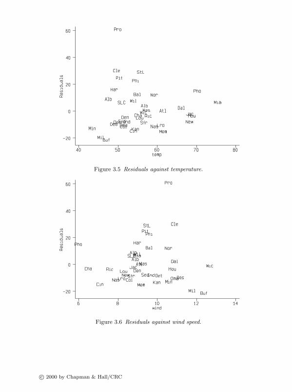
Figure 3.5 Residuals against temperature.

Figure 3.6 Residuals against wind speed.


Figure 3.7 Residuals against precipitation.

The simple residuals plotted by rvfplot and rvpplot have a distributionthat is scale dependent since the variance of each is a function of both σ2 andthe diagonal values of the so-called ‘hat’ matrix, H, given by:

H = X(X′X)−1X′ (3.5)(see Cook and Weisberg (1982), for a full explanation of the hat matrix).Consequently, it is often more useful to work with a standardized version, ri,calculated as follows:

ri =yi − yi

s√

1 − hii

(3.6)

where s2 is the estimate of σ2, yi is the predicted value of the response and hii

is the ith diagonal element of H.These standardized residuals can be obtained by applying the predict in-

struction. For example, to obtain a normal probability plot of the standardizedresiduals and to plot them against the fitted values requires the following in-structions:

predict fitpredict sdres, rstandardpnorm sdres, gap(5)graph sdres fit, symbol([town]) tr(3) ps(150) xlab ylab gap(3)

The first instruction stores the fitted values in the variable fit, the secondstores the standardized residuals in the variable sdres, the third produces a


Figure 3.8 Normal probability plot of standardized residuals.

normal probability plot (Figure 3.8), and the last instruction produces thegraph of standardized residuals against fitted values, which is shown in Fig-ure 3.9.

The normal probability plot indicates that the distribution of the residualsdeparts somewhat from normality. The pattern in the plot shown in Figure 3.9is identical to that in Figure 3.3 but here values outside (-2,2) indicate possibleoutliers; in this case the point corresponding to the town Providence. Analogousplots to those in Figures 3.4 to 3.7 could be obtained in the same way.

A rich variety of other diagnostics for investigating fitted regression mod-els have been developed during the last decade and many of these are avail-able with the regress procedure. Illustrated here is the use of two of these,namely the partial residual plot (Mallows (1986) and Cook’s distance statistic(Cook, 1977, 1979). The former are useful in identifying whether, for example,quadratic or higher order terms are needed for any of the explanatory variables;the latter measures the change to the estimates of the regression coefficientsthat results from deleting each observation and can be used to indicate thoseobservations that may be having an undue influence on the estimation andfitting process.

The partial residual plots are obtained using the cprplot command. Forthe four explanatory variables in the selected model for the pollution data, therequired plots are obtained as follows:

cprplot pop, border c(k) xlab ylab gap(4) /*


Figure 3.9 Standardized residuals against predicted values.

*/ l1("Partial Residuals")cprplot temp, border c(k) xlab ylab gap(4) /*

*/ l1("Partial Residuals")cprplot wind, border c(k) xlab ylab gap(4) /*

*/ l1("Partial Residuals")cprplot precip, border c(k) xlab ylab gap(4) /*

*/ l1("Partial Residuals")

The two graph options used, border and c(k), produce a border for the graphsand a locally weighted regression curve or lowess. The resulting graphs areshown in Figures 3.10 to 3.13. The graphs have to be examined for nonlinear-ities and whether the regression line, which has slope equal to the estimatedeffect of the corresponding explanatory variable in the chosen model, fits thedata adequately. The added lowess curve is generally helpful for both. None ofthe four graphs give any obvious indication of nonlinearity.

The Cook’s distance statistics are found by again using the predict in-struction; the following calculates these statistics for the chosen model for thepollution data and lists the observations where the statistic is greater than 4/40(4/n), which is usually the value regarded as indicating possible problems.

predict cook, cooksdlist town so2 cook if cook>4/40


Figure 3.10 Partial residual plot for population.

Figure 3.11 Partial residual plot for temperature.


Figure 3.12 Partial residual plot for wind speed.

Figure 3.13 Partial residual plot for precipitation.


town so2 cook1. Phoenix 10 .2543286

24. Philad 69 .368643729. Provid 94 .2839324

The first instruction stores the Cook’s distance statistics in the variable cookand the second lists details of those observations for which the statistic is abovethe suggested cut-off point.

There are three influential observations. Several of the diagnostic proceduresused previously also suggest these observations as possibly giving rise to prob-lems and some consideration should be given to repeating the analyses withthese three observations removed in addition to the initial removal of Chicago.

3.4 Exercises

1. Repeat the analyses described in this chapter after removing the three possi-ble outlying observations identified by the use of the Cook’s distance statis-tic.

2. The solution to the high correlation of the variables manuf and pop adoptedin the chapter was simply to remove the former. Investigate other possibili-ties such as defining a new variable manuf/pop in addition to pop to be usedin the regression analysis.

3. Consider the possibility of taking a transformation of sulphur dioxide pol-lution before undertaking any regression analyses. For example, try a logtransformation.

4. Explore the use of the many other diagnostic procedures available with theregress procedure.

See also exercises in Chapter 12.


CHAPTER 4

Analysis of Variance I: TreatingHypertension


Maxwell and Delaney (1990) describe a study in which the effects of 3 possibletreatments for hypertension were investigated. The details of the treatmentsare as follows:

Treatment Description Levelsdrug medication drug X, drug Y, drug Zbiofeed physiological feedback present, absentdiet special diet present, absent

All 12 combinations of the three treatments were included in a 3 × 2 × 2design. Seventy-two subjects suffering from hypertension were recruited and 6were allocated to each combination of treatments. Blood pressure measure-ments were made on each subject leading to the data shown in Table 4.1.

Table 4.1: Data in bp.raw

Biofeedback No Biofeedbackdrug X drug Y drug Z drug X drug Y drug Z

Diet absent170 186 180 173 189 202175 194 187 194 194 228165 201 199 197 217 190180 215 170 190 206 206160 219 204 176 199 224158 209 194 198 195 204

Diet present161 164 162 164 171 205173 166 184 190 173 199157 159 183 169 196 170152 182 156 164 199 160181 187 180 176 180 179190 174 173 175 203 179


Questions of interest concern differences in mean blood pressure for the differ-ent levels of the three treatments and the possibility of interactions betweenthe treatments.

4.2 Analysis of variance model

A suitable model for these data is

yijkl = µ+ αi + βj + γk + (αβ)ij + (αγ)ik + (βγ)jk + (αβγ)ijk + εijk (4.1)

where yijkl represents the blood pressure of the lth subject for the ith drug,the jth level of biofeedback, and the kth level of diet, µ is the overall mean,αi, βj and γk are the main effects for drugs, biofeedback and diets, αβ, αγ andβγ are the first order interaction terms, αβγ a is a second order interaction termand εijkl are the residual or error terms assumed to be normally distributedwith zero mean and variance σ2.


Assuming the data are in an ASCII file bp.raw, exactly as shown in Table 4.1,i.e., 12 rows, the first containing the observations 170 186 180 173 189 202,they can be read into Stata by producing a dictionary file, bp.dct containingthe following statements:

dictionary using bp.raw{_column(6) int bp11_column(14) int bp12_column(22) int bp13_column(30) int bp01_column(38) int bp02_column(46) int bp03

}

and using the following command

infile using bp

Note that it was not necesary to define a dictionary here since the sameresult could have been achieved using a simple infile command (see exercises).The final dataset should have a single variable, bp, that contains all the bloodpressures, and three additional variables, drug, biofeed, and diet representingthe corresponding levels of drug, biofeedback and diet.

First, create diet which should take on one value for the first six rows andanother for the following rows. This is achieved using the commands


gen diet=0 if _n<=6replace diet=1 if _n>6

or, more concisely, using

gen diet= n>6

Now use the reshape long command to stack the columns on top of eachother. If we specify bp0 and bp1 as the variable names in the reshape com-mand, then bp01, bp02, and bp03 are stacked into one column with variablename bp0 (and similarly for bp1) and another variable is created that containsthe suffixes 1, 2, and 3. We ask for this latter variable to be called drug usingthe option j(drug) as follows:

gen id=_nreshape long bp0 bp1, i(id) j(drug)list in 1/9

id drug diet bp0 bp11. 1 1 0 173 1702. 1 2 0 189 1863. 1 3 0 202 1804. 2 1 0 194 1755. 2 2 0 194 1946. 2 3 0 228 1877. 3 1 0 197 1658. 3 2 0 217 2019. 3 3 0 190 199

Here, id was generated because we needed to specify the row indicator inthe i() option.

We now need to run the reshape long command again to stack up thecolumns bp0 and bp1 and generate the variable biofeed. The instructions toachieve this and to label all the variables are given below.

replace id=_nreshape long bp, i(id) j(biofeed)replace id=_n

label drop _alllabel define d 0 "absent" 1 "present"label values diet dlabel values biofeed dlabel define dr 1 "Drug X" 2 "Drug Y" 3 "Drug Z"label values drug dr

To begin, it will be helpful to look at some summary statistics for each of thecells of the design. A simple way of obtaining the required summary measuresis to use the table instruction.


table drug, contents(freq mean bp median bp sd bp)/**/ by(diet biofeed)

----------+-----------------------------------------------diet, |biofeed |and drug | Freq. mean(bp) med(bp) sd(bp)----------+-----------------------------------------------absent |absent |

Drug X | 6 188 192 10.86278Drug Y | 6 200 197 10.07968Drug Z | 6 209 205 14.3527

----------+-----------------------------------------------absent |present |

Drug X | 6 168 167.5 8.602325Drug Y | 6 204 205 12.68069Drug Z | 6 189 190.5 12.61745

----------+-----------------------------------------------present |absent |

Drug X | 6 173 172 9.797959Drug Y | 6 187 188 14.01428Drug Z | 6 182 179 17.1114

----------+-----------------------------------------------present |present |

Drug X | 6 169 167 14.81891Drug Y | 6 172 170 10.93618Drug Z | 6 173 176.5 11.6619

----------+-----------------------------------------------

Display 4.1

The standard deviations in Display 4.1 indicate that there are considerabledifferences in the within cell variability. This may have implications for theanalysis of variance of these data since one of the assumptions made is thatthe observations within each cell have the same variance. To begin, however,apply the model specified in Section 3.2 to the raw data using the anovainstruction

anova bp drug diet biofeed diet*drug diet*biofeed /**/ drug*biofeed drug*diet*biofeed

The resulting ANOVA table is shown in Display 4.2.The Root MSE is simply the square root of the residual mean square, with

R-squared and Adj R-squared being as described in Chapter 3. The F-statisticof each effect represents the mean sum of squares for that effect, divided by theresidual mean sum of squares, given under the heading MS. The main effects ofdrug (F2,60 = 11.73, p < 0.001), diet (F1,60 = 33.20, p < 0.001), and biofeed


Number of obs = 72 R-squared = 0.5840Root MSE = 12.5167 Adj R-squared = 0.5077

Source | Partial SS df MS F Prob > F------------------+----------------------------------------------------

Model | 13194.00 11 1199.45455 7.66 0.0000|

drug | 3675.00 2 1837.50 11.73 0.0001diet | 5202.00 1 5202.00 33.20 0.0000

biofeed | 2048.00 1 2048.00 13.07 0.0006diet*drug | 903.00 2 451.50 2.88 0.0638

diet*biofeed | 32.00 1 32.00 0.20 0.6529drug*biofeed | 259.00 2 129.50 0.83 0.4425

drug*diet*biofeed | 1075.00 2 537.50 3.43 0.0388|

Residual | 9400.00 60 156.666667------------------+----------------------------------------------------

Total | 22594.00 71 318.225352

Display 4.2

(F1,60 = 13.07, p < 0.001) are all highly significant, and the three way interac-tion drug*diet*biofeed is also significant at the 5% level. The existence of athree-way interaction complicates the interpretation of the other terms in themodel; it implies that the interaction between any two of the factors is differ-ent at the different levels of the third factor. Perhaps the best way of tryingto understand the meaning of the three-way interaction is to plot a number ofinteraction diagrams; that is, plots of mean values for a factor at the differentlevels of the other factors.

This can be done by first creating a variable predbp containing the predictedmeans (which in this case coincide with the observed cell means because themodel is saturated) using the command

predict predbp

In order to produce a graph with separate lines for the factor diet, we needto generate the variables bp0 and bp1 as follows:

gen bp0=predbp if diet==0label variable bp0 "diet absent"gen bp1=predbp if diet==1label variable bp1 "diet present"

Plots of predbp against biofeed for each level of drug with seperate linesfor diet can be obtained using the instructions

sort druggraph bp0 bp1 biofeed, sort c(ll) by(drug) xlab(0,1) ylab /*

*/ b2(" ") b1("Blood pressure against biofeedback")


Figure 4.1 Interaction diagrams showing the interaction between diet and biofeedbackfor each level of drug.

The resulting interaction diagrams are shown in Figure 4.1. For drug Y, thepresence of biofeedback increases the effect of diet; whereas for drug Z theeffect of diet is hardly altered by the presence of biofeedback and for drug Xthe effect is decreased.

Tables of the cell means plotted in the interaction diagrams, as well as thecorresponding standard deviations, are produced for each drug using the fol-lowing command:

table diet biofeed, contents(mean bp sd bp) by(drug)

giving the outpit shown in Display 4.3.As mentioned previously, the observations in the 12 cells of the 3 × 2 × 2

design have variances which differ considerably. Consequently, an analysis ofvariance of the data transformed in some way might be worth considering. Forexample, to analyze the log transformed observations, we can use the followinginstructions:

gen lbp=log(bp)anova lbp drug diet biofeed diet*drug diet*biofeed /*

*/ drug*biofeed drug*diet*biofeed


----------+-------------------drug and | biofeeddiet | absent present----------+-------------------Drug X |

absent | 188 168| 10.86278 8.602325|

present | 173 169| 9.797959 14.81891

----------+-------------------Drug Y |

absent | 200 204| 10.07968 12.68069|

present | 187 172| 14.01428 10.93618

----------+-------------------Drug Z |

absent | 209 189| 14.3527 12.61745|

present | 182 173| 17.1114 11.6619

----------+-------------------

Display 4.3

Number of obs = 72 R-squared = 0.5776Root MSE = .068013 Adj R-squared = 0.5002

Source | Partial SS df MS F Prob > F-----------+----------------------------------------------------

Model | .379534762 11 .03450316 7.46 0.0000|

diet | .149561559 1 .149561559 32.33 0.0000drug | .107061236 2 .053530618 11.57 0.0001

biofeed | .061475507 1 .061475507 13.29 0.0006diet*drug | .024011594 2 .012005797 2.60 0.0830

diet*biofeed | .000657678 1 .000657678 0.14 0.7075drug*biofeed | .006467873 2 .003233936 0.70 0.5010

diet*drug*biofeed | .030299315 2 .015149657 3.28 0.0447|

Residual | .277545987 60 .004625766-----------+----------------------------------------------------

Total | .657080749 71 .009254658

The result is similar to the untransformed blood pressures. Since the threeway interaction is only marginally significant and if no substantive explanationof this interaction is available, it might be better to interpret the results interms of the very significant main effects. The relevant summary statisticsfor the log transformed blood pressures can be obtained using the followinginstructions:


table drug, contents(mean lbp sd lbp)

----------+-----------------------drug | mean(lbp) sd(lbp)

----------+-----------------------Drug X | 5.159152 .075955Drug Y | 5.247087 .0903675Drug Z | 5.232984 .0998921

----------+-----------------------

table diet, contents(mean lbp sd lbp)

----------+-----------------------diet | mean(lbp) sd(lbp)

----------+-----------------------absent | 5.258651 .0915982

present | 5.167498 .0781686----------+-----------------------

table biofeed, contents(mean lbp sd lbp)

----------+-----------------------biofeed | mean(lbp) sd(lbp)

----------+-----------------------absent | 5.242295 .0890136

present | 5.183854 .0953618----------+-----------------------

Drug X appears to produce lower blood pressures as does the special dietand the presence of biofeedback. Readers are encouraged to try other transfor-mations.

Note that the model with main effects only can also be estimated usingregression with dummy variables. Since drug has three levels and thereforerequires two dummy variables, we save some time by using the xi: prefix asfollows:

xi: regress lbp i.drug i.diet i.biofeed


i.drug Idrug_1-3 (naturally coded; Idrug_1 omitted)i.diet Idiet_0-1 (naturally coded; Idiet_0 omitted)i.biofeed Ibiofe_0-1 (naturally coded; Ibiofe_0 omitted)


Model | .318098302 4 .079524576 Prob > F = 0.0000Residual | .338982447 67 .00505944 R-squared = 0.4841---------+------------------------------ Adj R-squared = 0.4533

Total | .657080749 71 .009254658 Root MSE = .07113

------------------------------------------------------------------------------lbp | Coef. Std. Err. t P>|t| [95% Conf. Interval]

---------+--------------------------------------------------------------------Idrug_2 | .0879354 .0205334 4.283 0.000 .0469506 .1289203Idrug_3 | .0738315 .0205334 3.596 0.001 .0328467 .1148163Idiet_1 | -.0911536 .0167654 -5.437 0.000 -.1246175 -.0576896

Ibiofe_1 | -.0584406 .0167654 -3.486 0.001 -.0919046 -.0249767_cons | 5.233949 .0187443 279.228 0.000 5.196535 5.271363

------------------------------------------------------------------------------

The coefficients represent the mean differences between each level comparedwith the reference level (the omitted categories drug X, diet absent andbiofeedback absent) when the other variables are held constant. Due to thebalanced nature of the design (see next chapter), the p-values are equal tothose of ANOVA except that no overall p-value for drug is given. This can beobtained using

testparm Idrug*

( 1) Idrug_2 = 0.0( 2) Idrug_3 = 0.0

F( 2, 67) = 10.58Prob > F = 0.0001

The F-statistic is different than the one in the last anova command because nointeractions were included in the model so that the residual degrees of freedomand the residual sum of squares are both greater than before.

4.4 Exercises

1. Reproduce the result of the command infile using bp without using thedictionary and follow the reshape instructions to generate the requireddataset.

2. Produce three diagram with boxplots (1) for each level of drug, (2) for eachlevel of diet and (3) for each level of biofeedback.

3. Investigate other possible transformations of the data.4. Suppose that in addition to the blood pressure of each of the individuals in

the study, the investigator had also recorded their ages in file age.dat with


Table 4.2: Ages in age.dat to be used as a covariate

id age id age

1 39 37 452 39 38 583 61 39 614 50 40 475 51 41 676 43 42 497 59 43 548 50 44 489 47 45 4610 60 46 6711 77 47 5612 57 48 5413 62 49 6614 44 50 4315 63 51 4716 77 52 3517 56 53 5018 62 54 6019 44 55 7320 61 56 4621 66 57 5922 52 58 6523 53 59 4924 54 60 5225 40 61 4026 62 62 8027 68 63 4628 63 64 6329 47 65 5630 70 66 5831 57 67 5332 51 68 5633 70 69 6434 57 70 5735 64 71 6036 66 72 48

the results shown in Table 4.2. Reanalyze the data using age as a covariate(see help merge and help anova).


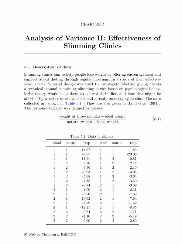
CHAPTER 5

Analysis of Variance II: Effectiveness ofSlimming Clinics


Slimming clinics aim to help people lose weight by offering encouragement andsupport about dieting through regular meetings. In a study of their effective-ness, a 2×2 factorial design was used to investigate whether giving clientsa technical manual containing slimming advice based on psychological behav-iorist theory would help them to control their diet, and how this might beaffected by whether or not a client had already been trying to slim. The datacollected are shown in Table 5.1. (They are also given in Hand et al, 1994).The response variable was defined as follows:

weight at three months − ideal weightnatural weight − ideal weight

(5.1)

Table 5.1: Data in slim.dat

cond status resp cond status resp

1 1 -14.67 1 1 -1.851 1 -8.55 1 1 -23.031 1 11.61 1 2 0.811 2 2.38 1 2 2.741 2 3.36 1 2 2.101 2 -0.83 1 2 -3.051 2 -5.98 1 2 -3.641 2 -7.38 1 2 -3.601 2 -0.94 2 1 -3.392 1 -4.00 2 1 -2.312 1 -3.60 2 1 -7.692 1 -13.92 2 1 -7.642 1 -7.59 2 1 -1.622 1 -12.21 2 1 -8.852 2 5.84 2 2 1.712 2 -4.10 2 2 -5.192 2 0.00 2 2 -2.80


The number of observations in each cell of the design is not the same, sothis is an example of a unbalanced 2×2 design.

5.2 Analysis of variance model

A suitable analysis of variance model for the data is

yijk = µ+ αi + βj + γij + εijk (5.2)

where yijk represents the weight change of the kth individual having status jand condition i, µ is the overall mean, αi represents the effect of condition i,βj the effect of status j, γij the status × condition interaction and εijk theresiduals–these are assumed to have a normal distribution with variance σ2.

The unbalanced nature of the slimming data presents some difficulties foranalysis not encountered in factorial designs having the same number of ob-servations in each cell (see the previous chapter). The main problem is thatwhen the data are unbalanced there is no unique way of finding a ‘sum ofsquares’ corresponding to each main effect and their interactions, since theseeffects are no longer independent of one another. If the data were balanced, theamong cells sum of squares would partition orthogonally into three componentsums of squares representing the two main effects and their interaction. Sev-eral methods have been proposed for dealing with this problem and each leadsto a different partition of the overall sum of squares. The different methodsfor arriving at the sums of squares for unbalanced designs can be explainedin terms of the comparisons of different sets of specific models. For a designwith two factors A and B, Stata can calculate the following types of sums ofsquares.

5.2.1 Sequential sums of squares

Sequential sums of squares (also known as hierarchical) represent the effect ofadding a term to an existing model. So, for example, a set of sequential sumsof squares such as

Source SSA SSAB SSB|AAB SSAB|A,B

represent a comparison of the following models:

• SSAB|A,B—model including an interaction and main effects compared withone including only main effects.

• SSB|A—model including both main effects, but with no interaction, com-pared with one including only the main effects of factor A.


• SSA—model containing only the A main effect compared with one contain-ing only the overall mean.

The use of these sums of squares in a series of tables in which the effects areconsidered in different orders (see later) will often provide the most satisfactoryway of deciding which model is most appropriate for the observations. (Theseare SAS Type I sums of squares—see Everitt and Der, 1996.)

5.2.2 Unique sums of squares

By default, Stata produces unique sums of squares that represent the contribu-tion of each term to a model including all the other terms. So, for a two-factordesign, the sums of squares represent the following.

Source SSA SSA|B,ABB SSB|A,ABAB SSAB|A,B

(These are SAS Type III sums of squares.) Note that these sums of squaresgenerally do not add up to the total sums of squares.

5.2.3 Regression

As we have shown in Chapter 4, ANOVA models may also be estimated usingregression by defining suitable dummy variables. Assume that A is representedby a single dummy variable. The regression coefficients for A represents thepartial contribution of that variable, adjusted for all other variables in themodel, say B. This is equivalent to the contribution of A to a model alreadyincluding B. A complication with regression models is that, in the presenceof an interaction, the p-values of the terms depend on the exact coding of thedummy variables (see Aitkin, 1978). The unique sums of squares correspond toregression where dummy variables are coded in a particular way, for examplea two-level factor can be coded as -1,1.

There have been numerous discussions over which sums of squares are mostappropriate for the analysis of unbalanced designs. The Stata manual appearsto recommend its default for general use. Nelder (1977) and Aitkin (1978)however, are strongly critical of ‘correcting’ main effects for an interactionterm involving the same factor; their criticisms are based on both theoreticaland pragmatic arguments and seem compelling. A frequently used approachis therefore to test the highest order interaction adjusting for all lower orderinteractions and not vice versa. Both Nelder and Aitkin prefer the use of Type Isums of squares in association with different orders of effects as the proceduremost likely to identify an appropriate model for a data set. For a detailedexplanation of the various types of sums of squares, see Boniface (1995).



The data can be read in from an ASCII file, slim.dat in the usual way using

infile cond status resp using slim.dat

A table showing the unbalanced nature of the 2×2 design can be obtainedfrom

tabulate cond status

| statuscond | 1 2 | Total

-----------+----------------------+----------1 | 5 12 | 172 | 11 6 | 17

-----------+----------------------+----------Total | 16 18 | 34

We now use the anova command with no options specified to obtain theunique (Type III) sums of squares:

anova resp cond status cond*status


Source | Partial SS df MS F Prob > F-----------+----------------------------------------------------

Model | 287.231861 3 95.7439537 2.66 0.0659|

cond | 2.19850409 1 2.19850409 0.06 0.8064status | 265.871053 1 265.871053 7.39 0.0108

cond*status | .130318264 1 .130318264 0.00 0.9524|

Residual | 1078.84812 30 35.961604-----------+----------------------------------------------------

Total | 1366.07998 33 41.3963631

Our recommendation is that the sums of squares shown in this table are notused to draw inferences because the main effects have been adjusted for theinteraction.

Instead we prefer an analysis that consists of obtaining two sets of sequentialsums of squares, the first using the order cond status cond*status and thesecond the order status cond cond*status; the necessary instructions are

anova resp cond status cond*status, sequential



Source | Seq. SS df MS F Prob > F-----------+----------------------------------------------------

Model | 287.231861 3 95.7439537 2.66 0.0659|

cond | 21.1878098 1 21.1878098 0.59 0.4487status | 265.913733 1 265.913733 7.39 0.0108

cond*status | .130318264 1 .130318264 0.00 0.9524|

Residual | 1078.84812 30 35.961604-----------+----------------------------------------------------

Total | 1366.07998 33 41.3963631

anova resp status cond cond*status, sequential


Source | Seq. SS df MS F Prob > F-----------+----------------------------------------------------

Model | 287.231861 3 95.7439537 2.66 0.0659|

status | 284.971071 1 284.971071 7.92 0.0085cond | 2.13047169 1 2.13047169 0.06 0.8094

cond*status | .130318264 1 .130318264 0.00 0.9524|

Residual | 1078.84812 30 35.961604-----------+----------------------------------------------------

Total | 1366.07998 33 41.3963631

The sums of squares corresponding to model and residuals are, of course, thesame in both tables, as is the sum of squares for the interaction term. Whatdiffers are the sums of squares in the cond and status rows in the two tables.The terms of most interest are the sum of squares of status|cond which isobtained from the table as 265.91, and the sum of squares of cond|statuswhich is 2.13. These sums of squares are less than the sums of squares forstatus and cond alone (284.97 and 21.19, respectively), by an amount of19.06, a portion of the sums of squares which cannot be uniquely attributedto either of the variables. The associated F-tests in the two tables make itclear that there is no interaction effect and that status|cond is significant butcond|status is not. The conclusion is that only status, i.e., whether or notthe woman had been slimming for over one year, is important in determiningweight change. Provision of the manual appears to have no discernible effect.

Results equivalent to the unique (Type III) sums of squares can be obtainedusing regression:

gen cond1=condrecode cond1 1=-1 2=1


gen status1=statusrecode status1 1=-1 2=1gen statcond = cond1*status1regress res cond1 status1 statcond



Total | 1366.07998 33 41.3963631 Root MSE = 5.9968

------------------------------------------------------------------------------resp | Coef. Std. Err. t P>|t| [95% Conf. Interval]

---------+--------------------------------------------------------------------cond1 | .2726251 1.102609 0.247 0.806 -1.979204 2.524454

status1 | 2.998042 1.102609 2.719 0.011 .746213 5.24987statcond | -.066375 1.102609 -0.060 0.952 -2.318204 2.185454

_cons | -3.960958 1.102609 -3.592 0.001 -6.212787 -1.70913------------------------------------------------------------------------------

These results differ from the regression used by Stata’s anova with the optionregress:

anova resp cond status cond*status, regress



Total | 1366.07998 33 41.3963631 Root MSE = 5.9968

------------------------------------------------------------------------------resp Coef. Std. Err. t P>|t| [95% Conf. Interval]

------------------------------------------------------------------------------_cons -.7566666 2.448183 -0.309 0.759 -5.756524 4.24319cond

1 -.4125001 2.9984 -0.138 0.891 -6.536049 5.7110492 (dropped)

status1 -5.863333 3.043491 -1.927 0.064 -12.07897 .35230442 (dropped)

cond*status1 1 -.2655002 4.410437 -0.060 0.952 -9.272815 8.7418151 2 (dropped)2 1 (dropped)2 2 (dropped)

------------------------------------------------------------------------------

because this uses different dummy variables. The dummy variables are equalto 1 for the levels to the left of the reported coefficient and zero otherwise, i.e.,the dummy variable for cond*status is one when status and cond are both1.


A table of mean values helpful in interpreting these results can be foundusing

table cond status, c(mean resp) row col f(%8.2f)

----------+--------------------| status

cond | 1 2 Total----------+--------------------

1 | -7.30 -1.17 -2.972 | -6.62 -0.76 -4.55

|Total | -6.83 -1.03 -3.76

----------+--------------------

The means demonstrate that experienced slimmers achieve the greatestweight reduction.

5.4 Exercises

1. Investigate what happens to the sequential sums of squares if the cond*statusinteraction term is given before the main effects cond status in the anovacommand with the sequential option.

2. Use regress to reproduce the analysis of variance by coding both conditionand status as (0,1) dummy variables and creating an interaction variable asthe product of these dummy variables.

3. Use regress in conjunction with xi: to fit the same model without theneed to generate any dummy variables (see help xi:).

4. Reproduce the results of anova resp cond status cond*status, regressusing regress by making xi: omit the last category instead of the first (seehelp xi).

See also the exercises in Chapters 7 and 13.


CHAPTER 6

Logistic Regression: Treatment of LungCancer and Diagnosis of Heart Attacks


Two datasets will be analyzed in this chapter. The first dataset shown in Ta-ble 6.1 originates from a clinical trial in which lung cancer patients were ran-domized to receive two different kinds of chemotherapy (sequential therapy andalternating therapy). The outcome was classified into one of four categories:progressive disease, no change, partial remission, or complete remission. Thedata were published in Holtbrugge and Schumacher (1991) and also appear inHand et al (1994). The main aim of any analysis will be to assess differencesbetween the two therapies.

Table 6.1: Tumor Data

Progressive No Partial CompleteTherapy Sex disease change remission remission

Sequential Male 28 45 29 26Female 4 12 5 2

Alternative Male 41 44 20 20Female 12 7 3 1

The second dataset in this chapter arises from a study to investigate the useof Serum Creatine Kinase (CK) levels for the diagnosis of myocardial infarction(heart attack). Patients admitted to a coronary care unit because they weresuspected of having had a myocardial infarction within the last 48 hours hadtheir CK levels measured on admission and the next two mornings. A clinicianwho was “blind” to the CK results came to an independent “gold standard”diagnosis using electrocardiograms, clinical records and autopsy reports. Themaximum CK levels for 360 patients are given in Table 6.2 together with theclinician’s diagnosis. The table was taken from Sackett et al (1991), whereonly the ranges of CK levels were given, not their precise values.

The main question of interest here is how well CK discriminates betweenthose with and without myocardial infarction and to investigate the charac-teristics of the diagnostic test for different thresholds.


Table 6.2: Diagnosis of myocardial infarction from Serum Creatine Kinase(CK)(Taken from Sackett et al (1991) with permission of the publisher, LittleBrown & Company)

Maximum CK Infarct Infarctlevel present absent

0-39 2 8840-79 13 2680-119 30 8120-159 30 5160-199 21 0200-239 19 1240-279 18 1280-319 13 1320-359 19 0360-399 15 0400-439 7 0440-479 8 0480- 35 0

6.2 The logistic regression model

Logistic regression is used when the response variable is dichotomous. In thiscase, we are interested in how the probability that the response variable takeson the value of interest (usually coded as 1, the other value being zero) dependson a number of explanatory variables. The probability π that y = 1 is just theexpected value of y. In linear regression (see Chapter 2), the expected value ofy is modeled as a linear function of the explanatory variables,

E[y] = β0 + β1x1 + β2x2 + · · · + βpxp. (6.1)

However, there are two problems with using the method of linear regressionwhen y is dichotomous: (1) the predicted probability must satisfy 0 ≤ π ≤ 1whereas a linear predictor can yield any value from minus infinity to plusinfinity, and (2) the observed values of y do not follow a normal distributionwith mean π, but rather a Bernoulli (or Binomial(1,π)) distribution.

In logistic regression, the first problem is addressed by replacing the prob-ability π = E[y] on the left hand side of equation (6.1) by the logit of theprobability, giving

logit(π) = log(π/(1 − π)) = β0 + β1x1 + β2x2 + · · · + βpxp. (6.2)

The logit of the probability is simply the log of the odds of the event of interest.Writing β and xi for the column vectors (β0, · · · , βp)T and (1, x1i, · · · , xpi)T ,


respectively, the predicted probability as a function of the linear predictor is

π(βT xi) =exp(βT xi)

1 + exp(βT xi)

=1

1 + exp(−βT xi). (6.3)

When the logit takes on any real value, this probability always satisfies 0 ≤π(βT xi) ≤ 1.

The second problem relates to the estimation procedure. Whereas maximumlikelihood estimation in linear regression leads to (weighted) least squares, thisis not the case in logistic regression. The log likelihood function for logisticregression is

l(β;y) =∑

i

[yi log(π(βT xi)) + (1 − yi) log(1 − π(βT xi))]. (6.4)

This log likelihood is maximized numerically using an iterative algorithm.For full details of logistic regression, see for example Collett (1991).

Logistic regression can be generalized to the situation where the responsevariable has more than two ordered response categories y1, · · · , yI by thinkingof these categories as resulting from thresholding an unobserved continuousvariable S = βT x + u at a number of cut-points κj , j = 1, · · · , I − 1 so thaty = y1 if S ≤ κ1, y = y2 if κ1 < S ≤ κ2, ... and y = yI if κI−1 < S. Thevariable u is assumed to have the standard logistic distribution Pr(u ≤ X) =1/(1+exp(−X)) so that the cumulative probability γj of a response up to andincluding yj , Pr(y ≤ yj), is

γj = Pr(S ≤ κj) = Pr(S − βT x ≤ κj − βT x)

=1

1 + exp(βT x − κj)(6.5)

where κI is taken to be ∞ so that γI = 1. The probability of the jth responsecategory is then simply πj = γj − γj−1.

The ordinal regression model is called the proportional odds model becausethe log odds that y > yj is

log(1 − γj(x)γj(x)

) = βT x − κj (6.6)

so that the log odds ratio for two values of x is βT (x1−x2) and is independentof j. Therefore, exp(βk) is the odds ratio that y > yj for any j when xk

increases by 1.In ordinary logistic regression, y1 = 0, y2 = 1, κ1 = 0 and exp(βk) is the

odds ratio that y = 1 when xk increases by 1.Note that the probit and ordinal probit models correspond to logistic and


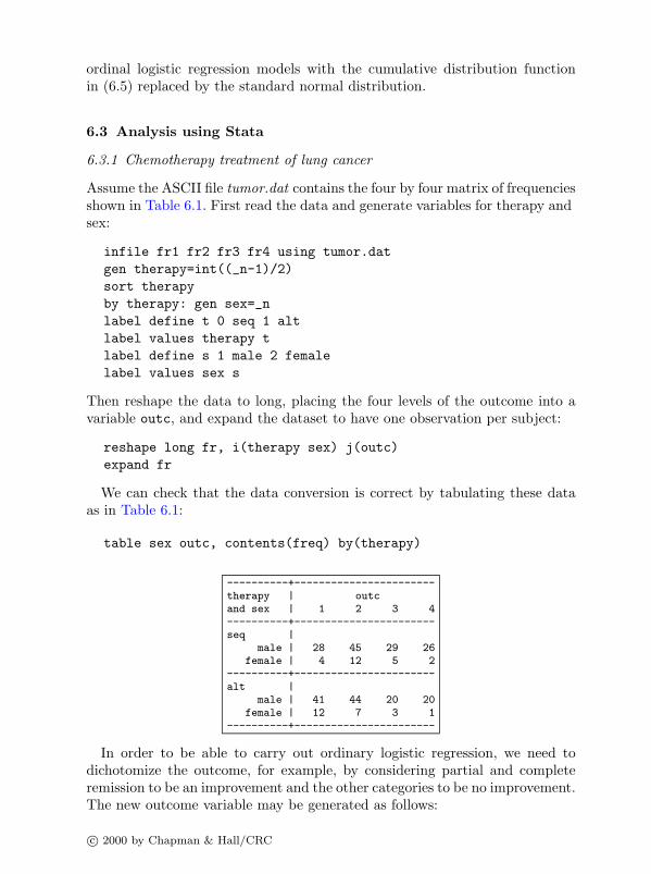
ordinal logistic regression models with the cumulative distribution functionin (6.5) replaced by the standard normal distribution.


6.3.1 Chemotherapy treatment of lung cancer

Assume the ASCII file tumor.dat contains the four by four matrix of frequenciesshown in Table 6.1. First read the data and generate variables for therapy andsex:

infile fr1 fr2 fr3 fr4 using tumor.datgen therapy=int((_n-1)/2)sort therapyby therapy: gen sex=_nlabel define t 0 seq 1 altlabel values therapy tlabel define s 1 male 2 femalelabel values sex s

Then reshape the data to long, placing the four levels of the outcome into avariable outc, and expand the dataset to have one observation per subject:

reshape long fr, i(therapy sex) j(outc)expand fr

We can check that the data conversion is correct by tabulating these dataas in Table 6.1:

table sex outc, contents(freq) by(therapy)

----------+-----------------------therapy | outcand sex | 1 2 3 4----------+-----------------------seq |

male | 28 45 29 26female | 4 12 5 2

----------+-----------------------alt |

male | 41 44 20 20female | 12 7 3 1

----------+-----------------------

In order to be able to carry out ordinary logistic regression, we need todichotomize the outcome, for example, by considering partial and completeremission to be an improvement and the other categories to be no improvement.The new outcome variable may be generated as follows:


gen improve=outcrecode improve 1/2=0 3/4=1

The command logit for logistic regression follows the same syntax as regressand all other estimation commands. For example, automatic selection proce-dures can be carried out using sw and post-estimation commands such astestparm are available. First, include therapy as the only explanatory vari-able:

logit improve therapy

Iteration 0: Log Likelihood =-194.40888Iteration 1: Log Likelihood =-192.30753Iteration 2: Log Likelihood =-192.30471

Logit Estimates Number of obs = 299chi2(1) = 4.21Prob > chi2 = 0.0402

Log Likelihood = -192.30471 Pseudo R2 = 0.0108

------------------------------------------------------------------------------improve | Coef. Std. Err. z P>|z| [95% Conf. Interval]

---------+--------------------------------------------------------------------therapy | -.4986993 .2443508 -2.041 0.041 -.977618 -.0197805

_cons | -.361502 .1654236 -2.185 0.029 -.6857263 -.0372777------------------------------------------------------------------------------

The algorithm takes three iterations to converge. The coefficient of therapyrepresents the difference in the log odds (of an improvement) between the alter-nating and sequential therapies. The negative value indicates that sequentialtherapy is superior to alternating therapy. The p-value of the coefficient is 0.041in the table. This was derived from the Wald-statistic, z, which is equal to thecoefficient divided by its asymptotic standard error (Std. Err.) as derivedfrom the Hessian matrix of the log likelihood function, evaluated at the max-imum likelihood solution. This p-value is less reliable than the p-value basedon the likelihood ratio between the model including only the constant andthe current model, which is given at the top of the output (chi2(1)=4.21).Here, minus twice the log of the likelihood ratio is equal to 4.21 which has anapproximate χ2-distribution with one degree of freedom (because there is oneadditional parameter) giving a p-value of 0.040, very similar to that based onthe Wald-test. The coefficient of therapy represents the difference in log oddsbetween the therapies and is not easy to interpret apart from the sign. Takingthe exponential of the coefficient gives the odds ratio and exponentiating the95% confidence limits gives the confidence interval for the odds ratio. Fortu-nately, the command logistic may be used to obtain the required odds ratioand its confidence interval


logistic improve therapy



------------------------------------------------------------------------------improve | Odds Ratio Std. Err. z P>|z| [95% Conf. Interval]

---------+--------------------------------------------------------------------therapy | .6073201 .1483991 -2.041 0.041 .3762061 .9804138

------------------------------------------------------------------------------

The standard error now represents the approximate standard error of the oddsratio (calculated using the delta method). However, the Wald statistic andconfidence interval are derived using the log odds and its standard error asthe sampling distribution of the log odds is much closer to normal than thatof the odds. In order to be able to test whether the inclusion of sex in the modelsignificantly increases the likelihood, the current likelihood can be saved using

lrtest, saving(1)

Including sex gives

logistic improve therapy sex



------------------------------------------------------------------------------improve | Odds Ratio Std. Err. z P>|z| [95% Conf. Interval]

---------+--------------------------------------------------------------------therapy | .6051969 .1486907 -2.044 0.041 .3739084 .9795537

sex | .5197993 .1930918 -1.761 0.078 .2509785 1.076551------------------------------------------------------------------------------

The p-value of sex based on the Wald-statistic is 0.078 and a p-value for thelikelihood ratio test is obtained using

lrtest, saving(0)lrtest, model(1) using(0)

Logistic: likelihood-ratio test chi2(1) = 3.35Prob > chi2 = 0.0674

which is not very different to the value of 0.078. Note that model(1) refersto the model which is nested in the more complicated model referred to byusing(0). If the two models had been fitted in the reverse order, it would nothave been necessary to specify these options because lrtest assumes that the


current model is nested in the last model saved using lrtest, saving(0).Retaining the variable sex in the model, the predicted probabilities can beobtained using

predict prob

and the four different predicted probabilites may be compared with the ob-served proportions as follows:

table sex , contents(mean prob mean improve freq) by(therapy)

----------+--------------------------------------------therapy |and sex | mean(prob) mean(improve) Freq.----------+--------------------------------------------seq |

male | .4332747 .4296875 128female | .2843846 .3043478 23

----------+--------------------------------------------alt |

male | .3163268 .32 125female | .1938763 .173913 23

----------+--------------------------------------------

The agreement is good, so there appears to be no strong interaction betweensex and type of therapy. (We could test for an interaction between sex andtherapy by using xi: logistic improve i.therapy*i.sex). Residuals arenot very informative for these data because there are only four different pre-dicted probabilities.

We now fit the proportional odds model using the full ordinal response vari-able outc:

ologit outc therapy sex, table

The results are shown in Display 6.1. Both therapy and sex are more sig-nificant than before. The coefficients represent the log odds ratios of being incomplete remission versus being at best in partial remission; or equivalently,the log odds ratio of being at least in partial remission rather than havingprogressive disease or no change. The option table has produced the last partof the output to remind us how the proportional odds model is defined. Wecould calculate the probability that a male (sex=1) who is receiving sequentialtherapy (therapy=0) will be in complete remission (outc=4) using 1−γ3 (seeequation (6.5))

display 1-1/(1+exp(-0.5413938-0.758662))

.21415563

However, a much quicker way of computing the predicted probabilities forall four responses and all combinations of explanatory variables is to use thecommand predict


Iteration 0: Log Likelihood =-399.98398Iteration 1: Log Likelihood =-394.53988Iteration 2: Log Likelihood =-394.52832

Ordered Logit Estimates Number of obs = 299chi2(2) = 10.91Prob > chi2 = 0.0043


------------------------------------------------------------------------------outc | Coef. Std. Err. z P>|z| [95% Conf. Interval]

---------+--------------------------------------------------------------------therapy | -.580685 .2121432 -2.737 0.006 -.9964781 -.164892

sex | -.5413938 .2871764 -1.885 0.059 -1.104249 .0214616---------+--------------------------------------------------------------------

_cut1 | -1.859437 .3828641 (Ancillary parameters)_cut2 | -.2921603 .3672626_cut3 | .758662 .3741486

------------------------------------------------------------------------------

outc | Probability Observed---------|-------------------------------------

1 | Pr( xb+u<_cut1) 0.28432 | Pr(_cut1<xb+u<_cut2) 0.36123 | Pr(_cut2<xb+u<_cut3) 0.19064 | Pr(_cut3<xb+u) 0.1639

Display 6.1

predict p1 p2 p3 p4

and to tabulate the results as follows:

table sex, contents(mean p1 mean p2 mean p3 mean p4) by(therapy)

----------+-----------------------------------------------therapy |and sex | mean(p1) mean(p2) mean(p3) mean(p4)----------+-----------------------------------------------seq |

male | .2111441 .3508438 .2238566 .2141556female | .3150425 .3729235 .175154 .1368799

----------+-----------------------------------------------alt |

male | .3235821 .3727556 .1713585 .1323038female | .4511651 .346427 .1209076 .0815003

----------+-----------------------------------------------

6.3.2 Diagnosis of heart attacks

The data in sck.dat are read in using

infile ck pres abs using sck.dat


Each observation represents all subjects with maximum creatine kinase val-ues in the same range. The total number of subjects is pres+abs

gen tot=pres+abs

and the number of subjects with the disease is pres. The probability associatedwith each observation is Binomial(tot, π). The programs logit and logisticare for data where each observation represents a single Bernouilli trial, withprobability Binomial(1, π). Another program, blogit can be used to analyzethe “grouped” data with “denominators” tot:

blogit pres tot ck



------------------------------------------------------------------------------_outcome | Coef. Std. Err. z P>|z| [95% Conf. Interval]---------+--------------------------------------------------------------------

ck | .0351044 .0040812 8.601 0.000 .0271053 .0431035_cons | -2.326272 .2993611 -7.771 0.000 -2.913009 -1.739535

------------------------------------------------------------------------------

There is a very significant association between CK and the probability of in-farct. We now need to investigate whether it is reasonable to assume that thelog odds depends linearly on CK. Therefore, plot the observed proportions andpredicted probabilities as follows:

gen prop = pres/totpredict pred, plabel variable prop "observed"label variable pred "predicted"graph pred prop ck, c(s.) xlab ylab l1("Probability") gap(4)

The predict command gives predicted counts by default and therefore the poption was used to obtain predicted probabilities instead. The option c(s.) inthe graph command causes the first set of points to be connected by a smoothcurve. In the resulting graph in Figure 6.1, the curve fits the data reasonablywell, the largest discrepency being at CK=280.

We will now plot some residuals and then consider the sensitivity and speci-ficity of CK as a diagnostic tool for different thresholds. There are some usefulpost-estimation commands available for these purposes for use after logisticthat are not available after blogit. We therefore transform the data into theform required for logistic, i.e. one observation per Bernouilli trial with out-come infct equal to 0 or 1 so that the number of ones per CK level equalspres:


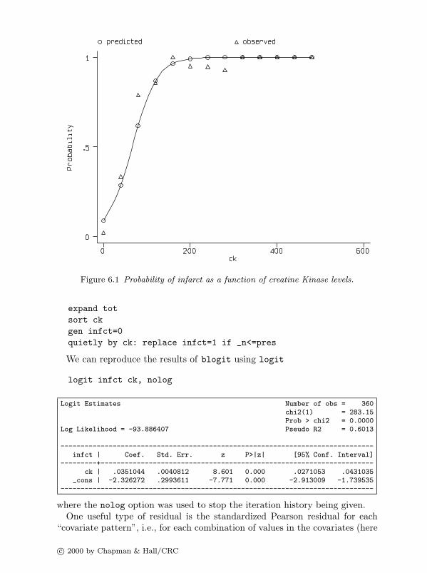
Figure 6.1 Probability of infarct as a function of creatine Kinase levels.

expand totsort ckgen infct=0quietly by ck: replace infct=1 if _n<=pres

We can reproduce the results of blogit using logit

logit infct ck, nolog



------------------------------------------------------------------------------infct | Coef. Std. Err. z P>|z| [95% Conf. Interval]

---------+--------------------------------------------------------------------ck | .0351044 .0040812 8.601 0.000 .0271053 .0431035

_cons | -2.326272 .2993611 -7.771 0.000 -2.913009 -1.739535------------------------------------------------------------------------------

where the nolog option was used to stop the iteration history being given.One useful type of residual is the standardized Pearson residual for each

“covariate pattern”, i.e., for each combination of values in the covariates (here


for each value of CK). These residuals may be obtained and plotted as follows:

predict resi, rstandardgraph resi ck, s([ck]) psize(150) xlab ylab gap(5)

The graph is shown in Figure 6.2. There are several large outliers. The largest

Figure 6.2 Standardized Pearson residuals vs creatine Kinase level.

outlier at CK=280 is due to one subject out of 14 not having had an infarctalthough the predicted probability of an infarct is almost 1.

We now determine the accuracy of the diagnostic test. A classification tableof the predicted diagnosis (using a cut-off of the predicted probability of 0.5)versus the true diagnosis may be obtained using

lstat

giving the table shown in Display 6.2. Both the sensitivity and specificity arerelatively high. These characteristics are generally assumed to generalize toother populations whereas the positive and negative predictive values dependon the prevalence (or prior probability) of the condition (for example, seeSackett et al, 1991).

The use of other probability cut-offs could be investigated using the optioncutoff(#) in the above command or using the commands lroc to plot a


Logistic model for infct

-------- True --------Classified | D ~D Total-----------+--------------------------+-----------

+ | 215 16 | 231- | 15 114 | 129

-----------+--------------------------+-----------Total | 230 130 | 360

Classified + if predicted Pr(D) >= .5True D defined as infct ~= 0--------------------------------------------------Sensitivity Pr( +| D) 93.48%Specificity Pr( -|~D) 87.69%Positive predictive value Pr( D| +) 93.07%Negative predictive value Pr(~D| -) 88.37%--------------------------------------------------False + rate for true ~D Pr( +|~D) 12.31%False - rate for true D Pr( -| D) 6.52%False + rate for classified + Pr(~D| +) 6.93%False - rate for classified - Pr( D| -) 11.63%--------------------------------------------------Correctly classified 91.39%--------------------------------------------------

Display 6.2

ROC-curve (specificity vs sensitivity for differenct cut-offs) or lsens to plotsensitivity and specificity against cut-off (see exercises).

The above classification table may be misleading because we are testing themodel on the same sample that was used to derive it. An alternative approachis to compute predicted probabilities for each observation from a model fittedto the remaining observations. This method, called “leave one out” methodor jacknifing (see Lachenbruch and Mickey, 1986), can be carried out rela-tively easily for our data because we only have a small number of covariateand response patterns. Instead of looping through all observations, excludingeach observation in the logistic regression command and computing that ob-servation’s predicted probability, we can loop through a subset of observationsrepresenting all combinations of covariates and responses found in the data.

First, label each unique covariate pattern consecutively in a variable numusing predict with the number option:

predict num, number

Now generate first, equal to one for the first observation in each group ofunique covariate and response patterns and zero otherwise:

sort num infctquietly by num infct : gen first = _n==1


Now define grp, equal to the cumulative sum of first, obtained using thefunction sum(). This variable numbers the groups of unique covariate andresponse patterns consecutively:

gen grp=sum(first)

(An alternative way of generating grp without having to first create firstwould be to use the command egen grp=group(num infct).) Now determinethe number of unique combinations of CK levels and infarct status:

summ grp

Variable | Obs Mean Std. Dev. Min Max---------+-----------------------------------------------------

grp | 360 8.658333 6.625051 1 20

Since there are 20 groups, we need to run logistic 20 times (for each valueof grp), excluding one observation from grp to derive the model for predictingthe probability for all observations in grp.

First generate a variable, nxt, that consecutively labels the 20 observationsto be excluded in turn:

gen nxt = 0replace nxt = grp if first==1

Now build up a variable prp of predicted probabilities as follows:gen prp=0for num 1/20:logistic infct ck if nxt~=X \ predict p \ /*

*/ replace prp=p if grp==X \ drop p

Here we used back-slashes to run four commands in each iteration of theloop, to1. derive the model excluding one observation from grp

2. obtain the predicted probabilities p ( predict produces results for the wholesample, not just the estimation sample)

3. set prp to the predicted probability for all observations in grp and4. drop p so that it can be defined again in the next iteration.

The classification table for the jacknifed probabilities can be obtained using

gen class=cond(prp>=0.5, 1, 0)tab class infct

| infctclass | 0 1 | Total

-----------+----------------------+----------0 | 114 15 | 1291 | 16 215 | 231

-----------+----------------------+----------Total | 130 230 | 360

giving the same result as before (this is not generally the case).


6.4 Exercises

1. Read in the data without using the expand command and reproduce theresult of ordinal logistic regressions by using the appropriate weights.

2. Test for an association between depress and life for the data described inChapter 2 using

(a) ordinal logistic regression with depress as dependent variable.(b) logisitc regression with life as dependent variable.

3. Use sw together with logistic to find a model for predicting life us-ing the data from Chapter 2 with different sets of candidate variables (seeChapter 3).

4. Produce a graph similar to that in Figure 6.1 using probit analysis (see helpfor bprobit).

5. Explore the use of lstat, cutoff(#), lroc and lsens for the diagnosisdata.


CHAPTER 7

Generalized Linear Models: AustralianSchool Children


This chapter reanalyzes a number of datasets discussed in previous chaptersand, in addition, describes the analysis of a new dataset given in Aitkin (1978) .These data come from a sociological study of Australian Aboriginal and whitechildren. The sample included children from four age groups (final year inprimary school and first three years in secondary school) who were classifiedas slow or average learners. The number of days absent from school during theschool year was recorded for each child. The data are given in Table 7.1. Thevariables are as follows:• eth: ethnic group (A=aboriginal, N=white)• sex: sex (M=male, F=female)• age: class in school (F0, F1, F2, F3)• lrn: average or slow learner(SL=slow learner, AL=average learner)• days: number of days absent from school in one year

7.2 Generalized linear models

Previous chapters have described linear and logistic regression. In this chapter,we will describe an even more general class of models, called generalized linearmodels, of which linear regression and logistic regression are special cases.

Both linear and logistic regression involve a linear combination of the ex-planatory variables, called the linear predictor, of the form

η = β0 + βx1 + βx2 + · · · + βxp

= βT x. (7.1)

In both types of regression, the linear predictor determines the expectation µof the response variable. In linear regression, where the response is continuous,µ is directly equated with the linear predictor. This is not advisable when theresponse is dichotomous because in this case the expectation is a probabilitywhich must satisfy 0 ≤ µ ≤ 1. In logistic regression, the linear predictor is


Table 7.1 Data in quine.dta presented in four columns to save space. (Taken fromAitkin (1978) with permission of the Royal Statistical Society)

eth sex age lrn days eth sex age lrn days eth sex age lrn days eth sex age lrn days

A M F0 SL 2 A M F0 SL 11 A M F0 SL 14 A M F0 AL 5A M F0 AL 5 A M F0 AL 13 A M F0 AL 20 A M F0 AL 22A M F1 SL 6 A M F1 SL 6 A M F1 SL 15 A M F1 AL 7A M F1 AL 14 A M F2 SL 6 A M F2 SL 32 A M F2 SL 53A M F2 SL 57 A M F2 AL 14 A M F2 AL 16 A M F2 AL 16A M F2 AL 17 A M F2 AL 40 A M F2 AL 43 A M F2 AL 46A M F3 AL 8 A M F3 AL 23 A M F3 AL 23 A M F3 AL 28A M F3 AL 34 A M F3 AL 36 A M F3 AL 38 A F F0 SL 3A F F0 AL 5 A F F0 AL 11 A F F0 AL 24 A F F0 AL 45A F F1 SL 5 A F F1 SL 6 A F F1 SL 6 A F F1 SL 9A F F1 SL 13 A F F1 SL 23 A F F1 SL 25 A F F1 SL 32A F F1 SL 53 A F F1 SL 54 A F F1 AL 5 A F F1 AL 5A F F1 AL 11 A F F1 AL 17 A F F1 AL 19 A F F2 SL 8A F F2 SL 13 A F F2 SL 14 A F F2 SL 20 A F F2 SL 47A F F2 SL 48 A F F2 SL 60 A F F2 SL 81 A F F2 AL 2A F F3 AL 0 A F F3 AL 2 A F F3 AL 3 A F F3 AL 5A F F3 AL 10 A F F3 AL 14 A F F3 AL 21 A F F3 AL 36A F F3 AL 40 N M F0 SL 6 N M F0 SL 17 N M F0 SL 67N M F0 AL 0 N M F0 AL 0 N M F0 AL 2 N M F0 AL 7N M F0 AL 11 N M F0 AL 12 N M F1 SL 0 N M F1 SL 0N M F1 SL 5 N M F1 SL 5 N M F1 SL 5 N M F1 SL 11N M F1 SL 17 N M F1 AL 3 N M F1 AL 4 N M F2 SL 22N M F2 SL 30 N M F2 SL 36 N M F2 AL 8 N M F2 AL 0N M F2 AL 1 N M F2 AL 5 N M F2 AL 7 N M F2 AL 16N M F2 AL 27 N M F3 AL 0 N M F3 AL 30 N M F3 AL 10N M F3 AL 14 N M F3 AL 27 N M F3 AL 41 N M F3 AL 69N F F0 SL 25 N F F0 AL 10 N F F0 AL 11 N F F0 AL 20N F F0 AL 33 N F F1 SL 5 N F F1 SL 7 N F F1 SL 0N F F1 SL 1 N F F1 SL 5 N F F1 SL 5 N F F1 SL 5N F F1 SL 5 N F F1 SL 7 N F F1 SL 11 N F F1 SL 15N F F1 AL 5 N F F1 AL 14 N F F1 AL 6 N F F1 AL 6N F F1 AL 7 N F F1 AL 28 N F F2 SL 0 N F F2 SL 5N F F2 SL 14 N F F2 SL 2 N F F2 SL 2 N F F2 SL 3N F F2 SL 8 N F F2 SL 10 N F F2 SL 12 N F F2 AL 1N F F3 AL 1 N F F3 AL 9 N F F3 AL 22 N F F3 AL 3N F F3 AL 3 N F F3 AL 5 N F F3 AL 15 N F F3 AL 18N F F3 AL 22 N F F3 AL 37


therefore equated with a function of µ, the logit, η = log(µ/(1−µ)). In gener-alized linear models, the linear predictor may be equated with any of a numberof different functions g(µ) of µ, called link functions; that is,

η = g(µ). (7.2)

In linear regression, the probability distribution of the response variable isassumed to be normal with mean µ. In logistic regression a binomial distribu-tion is assumed with probability parameter µ. Both distributions, the normaland Binomial distributions, come from the same family of distributions, calledthe exponential family,

f(y; θ, φ) = exp{(yθ − b(θ))/a(φ) + c(y, φ)}. (7.3)

For example, for the normal distribution,

f(y; θ, φ) =1√

(2πσ2)exp{−(y − µ)2/2σ2}

= exp{(yµ− µ2/2)/σ2 − 12(y2/σ2 + log(2πσ2))} (7.4)

so that θ = µ, b(θ) = θ2/2, φ = σ2 and a(φ) = φThe parameter θ, a function of µ, is called the canonical link. The canonical

link is frequently chosen as the link function (and is the default link in the Statacommand for fitting generalized linear models, glm) although the canonicallink is not necessarily more appropriate than any other link. Table 7.2 listssome of the most common distributions and their canonical link functionsused in generalized linear models. The mean and variance of Y are given by

Table 7.2: Probability distributions and their canonical link functions

Variance Dispersion LinkDistribution function parameter function g(µ) = θ(µ)

Normal 1 σ2 identity µBinomial µ(1 − µ) 1 logit log(µ/(1 − µ))Poisson µ 1 log ln(µ)Gamma µ2 ν−1 reciprocal 1/µ

E(Y ) = b′(θ) = µ (7.5)and

var(Y ) = b′′(θ)a(φ) = V (µ)a(φ) (7.6)where b′(θ) and b′′(θ) denote the fist and second derivative of b(θ) with respectto θ and the variance function V (µ) is obtained by expressing b′′(θ) as a func-tion of µ. It can be seen from (7.4) that the variance for the normal distribution


is simply σ2 regardless of the value of the mean µ, i.e., the variance functionis 1.

The data on Australian school children will be analyzed by assuming a Pois-son distribution for the number of days absent from school. The Poisson distri-bution is the appropriate distribution of the number of events observed, if theseevents occur independently in continuous time at a constant instantaneousprobability rate (or incidence rate), see for example Clayton and Hills (1993).The Poisson distribution is given by

f(y;µ) = µye−µ/y!, y = 0, 1, 2, · · · . (7.7)

Taking the logarithm and summing over observations, the log likelihood is

l(µ;y) =∑

i

{(yi lnµi − µi) − ln(yi!)} (7.8)

so that θ = lnµ, b(θ) = exp(θ), φ = 1, a(φ) = 1 and var(y) = exp(θ) = µ.Therefore, the variance of the Poisson distribution is not constant, but equalto the mean. Unlike the normal distribution, the Poisson distribution has noseparate parameter for the variance and the same is true of the Binomialdistribution. Table 7.2 shows the variance functions and dispersion parametersfor some commonly used probability distributions.

7.2.1 Model selection and measure of fit

Lack of fit may be expressed by the deviance, which is minus twice the dif-ference between the maximized log likelihood of the model and the maximumlikelihood achievable, i.e., the maximized likelihood of the full or saturatedmodel. For the normal distribution, the deviance is simply the residual sum ofsquares. Another measure of lack of fit is the generalized Pearson X2,

X2 =∑

i

(yi − µi)2/V (µi), (7.9)

which, for the Poisson distribution, is just the familiar statistic for two-waycross-tabulations (since V (µ) = µ). Both the deviance and Pearson X2 haveχ2 distributions when the sample size tends to infinity. When the dispersionparameter φ is fixed (not estimated), an analysis of deviance may be used fortesting nested models in the same way as analysis of variance is used for linearmodels. The difference in deviance between two models is simply comparedwith the χ2 distribution with degrees of freedom equal to the difference inmodel degrees of freedom.

The Pearson and deviance residuals are defined as the (signed) square rootsof the contributions of the individual observations to the Pearson X2 and de-viance respectively. These residuals may be used to assess the appropriatenessof the link and variance functions.

A relatively common phenomenon with binary and count data is overdis-persion, i.e., the variance is greater than that of the assumed distribution


(binomial and Poisson respectively). This overdispersion may be due to extravariability in the parameter µ which has not been completely explained by thecovariates. One way of addressing the problem is to allow µ to vary randomlyaccording to some (prior) distribution and to assume that conditional on theparameter having a certain value, the response variable follows the binomial(or Poisson) distribution. Such models are called random effects models.

A more pragmatic way of accommodating overdispersion in the model isto assume that the variance is proportional to the variance function, but toestimate the dispersion rather than assuming the value 1 appropriate for thedistributions. For the Poisson distribution, the variance is modelled as

var(Y ) = φµ (7.10)

where φ is estimated from the Deviance or Pearson X2. (This is analogousto the estimation of the residual variance in linear regresion models from theresidual sums of squares.) This parameter is then used to scale the estimatedstandard errors of the regression coefficients. If the variance is not proportionalto the variance function, robust standard errors can be used, see next section.This approach of assuming a variance function that does not correspond to anyprobability distribution is an example of quasi-likelihood, see also Chapter 9.

see McCullagh and Nelder (1989) for more details on generalized linear mod-els.

7.2.2 Robust standard errors of parameter estimates

A very useful feature of Stata is that robust standard errors of estimated pa-rameters can be obtained for many estimation commands. In maximum likeli-hood estimation, the standard errors of the estimated parameters are derivedfrom the Hessian of the log-likelihood. However, these standard errors are cor-rect only if the likelihood is the true likelihood of the data. If this assumptionis not correct, due to misspecification of the covariates, the link function, orthe probability distribution function, we can still use robust estimates of thestandard errors known as the Huber, White or sandwich variance estimates(for details, see Binder (1983) ).

In the description of the robust variance estimator in the Stata User’s Guide(Section 23.11), it is pointed out that the use of robust standard errors impliesa slightly less ambitious interpretation of the parameter estimates and theirstandard errors than a model-based approach. The parameter estimates areunbiased estimates of the estimates that would be obtained if we had an infinitesample (not of any true parameters), and their standard errors are the standarddeviations under repeated sampling followed by estimation (see also the FAQby Sribney, 1998).

Another approach to estimating the standard errors without making anydistributional assumptions is bootstrapping (Efron and Tibshirani, 1993). If we


could obtain repeated samples from the population (from which our data weresampled), we could obtain an empirical sampling distribution of the parameterestimates. In Monte-Carlo simulation, the required samples are drawn from theassumed distribution. In bootstrapping, the sample is resampled “to approx-imate what would happen if the population were sampled” (Manley, 1997) .Bootstrapping works as follows. Take a random sample of n observations, withreplacement, and estimate the regression coefficients. Repeat this a number oftimes to obtain a sample of estimates. From this sample, estimate the variance-covariance matrix of the parameter estimates. Confidence intervals may beconstructed using the estimated variance or directly from the appropriate cen-tiles of the empirical distribution of parameter estimates. See Manley (1997)and Efron and Tibshirani (1993) for more information on the bootsrap.


The glm command can be used to fit generalized linear models. The syntaxis analogous to logistic and regress except that the options family() andlink() are used to specify the probability distribution of the response and thelink function, respectively.

7.3.1 Datasets from previous chapters

First, we show how linear regression can be carried out using glm. In Chapter 3,the U. S. air-pollution data were read in using the instructions

infile str10 town so2 temp manuf pop wind precip days /**/ using usair.dat

drop if town=="Chicago"

and now we regress so2 on a number of variables using

glm so2 temp pop wind precip, fam(gauss) link(id)


Iteration 1 : deviance = 10150.1520

Residual df = 35 No. of obs = 40Pearson X2 = 10150.15 Deviance = 10150.15Dispersion = 290.0043 Dispersion = 290.0043

Gaussian (normal) distribution, identity link------------------------------------------------------------------------------

so2 | Coef. Std. Err. t P>|t| [95% Conf. Interval]---------+--------------------------------------------------------------------

temp | -1.810123 .4404001 -4.110 0.000 -2.704183 -.9160635pop | .0113089 .0074091 1.526 0.136 -.0037323 .0263501

wind | -3.085284 2.096471 -1.472 0.150 -7.341347 1.170778precip | .5660172 .2508601 2.256 0.030 .0567441 1.07529_cons | 131.3386 34.32034 3.827 0.001 61.66458 201.0126

------------------------------------------------------------------------------(Model is ordinary regression, use regress instead)

The results are identical to those of the regression analysis as the remark atthe bottom of the output points out. The dispersion parameter represents theresidual variance given under Residual MS in the analysis of variance table ofthe regression analysis in Chapter 3. We can estimate robust standard errorsusing regress with the option robust (the robust estimator is not yet availablefor glm although a Roger Newson has written a program rglm for this purpose,published in STB-50 sg114):

reg so2 temp pop wind precip, robust

Regression with robust standard errors Number of obs = 40F( 4, 35) = 9.72Prob > F = 0.0000R-squared = 0.3446Root MSE = 17.03

------------------------------------------------------------------------------| Robust

so2 | Coef. Std. Err. t P>|t| [95% Conf. Interval]---------+--------------------------------------------------------------------

temp | -1.810123 .3462819 -5.227 0.000 -2.513113 -1.107134pop | .0113089 .0084062 1.345 0.187 -.0057566 .0283743

wind | -3.085284 1.792976 -1.721 0.094 -6.72522 .554651precip | .5660172 .1919587 2.949 0.006 .1763203 .955714_cons | 131.3386 19.23291 6.829 0.000 92.29368 170.3835

------------------------------------------------------------------------------

giving slightly different standard errors which indicates that the assumptionof identically normally distributed residuals may not be entirely satisfied.

We now show how an analysis of variance model can be fitted using glm,using the slimming clinic example of chapter 5. The data are read using

infile cond status resp using slim.dat

and the full, saturated model may be obtained using


xi: glm resp i.cond*i.status, fam(gauss) link(id)

i.cond Icond_1-2 (naturally coded; Icond_1 omitted)i.status Istatu_1-2 (naturally coded; Istatu_1 omitted)i.cond*i.status IcXs_#-# (coded as above)




resp | Coef. Std. Err. t P>|t| [95% Conf. Interval]---------+--------------------------------------------------------------------Icond_2 | .6780002 3.234433 0.210 0.835 -5.927593 7.283594

Istatu_2 | 6.128834 3.19204 1.920 0.064 -.3901823 12.64785IcXs_2_2 | -.2655002 4.410437 -0.060 0.952 -9.272815 8.741815

_cons | -7.298 2.68185 -2.721 0.011 -12.77507 -1.820931------------------------------------------------------------------------------(Model is ordinary regression, use regress instead)

This result is identical to that obtained using the command

xi: regress resp i.cond*i.status

(see Chapter 5, Exercises).We can obtain the F-statistics for the interaction term by saving the deviance

of the above model (residual sum of squares) in a local macro and refitting themodel with the interaction removed:

local dev0=e(deviance)

xi: glm resp i.cond i.status, fam(gauss) link(id)

i.cond Icond_1-2 (naturally coded; Icond_1 omitted)i.status Istatu_1-2 (naturally coded; Istatu_1 omitted)




resp | Coef. Std. Err. t P>|t| [95% Conf. Interval]---------+--------------------------------------------------------------------Icond_2 | .5352102 2.163277 0.247 0.806 -3.876821 4.947242

Istatu_2 | 5.989762 2.167029 2.764 0.010 1.570077 10.40945_cons | -7.199832 2.094584 -3.437 0.002 -11.47176 -2.927901

------------------------------------------------------------------------------(Model is ordinary regression, use regress instead)


The increase in deviance caused by the removal of the interaction term rep-resents the sum of squares of the interaction term after eliminating the maineffects:

local dev1=e(deviance)local ddev=‘dev1’-‘dev0’display ‘ddev’

.13031826

and the F-statistic is simply the mean sum of squares of the interaction termafter eliminating the main effects divided by the residual mean square of thefull model. The numerator and denominator degrees of freedom are 1 and 30respectively so that F and the associated p-value may be obtained as follows:

local f=(‘ddev’/1)/(‘dev0’/30)display ‘f’

.00362382

display fprob(1,30,‘f’)

.95239706

The general method for testing the difference in fit of two nested generalizedlinear models, using the difference in deviance, is not appropriate here becausethe dispersion parameter φ = σ2 was estimated.

The logistic regression analysis of chapter 6 may also be repeated using glm.We first read the data as before, without replicating records.

infile fr1 fr2 fr3 fr4 using tumor.dat, cleargen therapy=int((_n-1)/2)sort therapyby therapy: gen sex=_nreshape long fr, i(therapy sex) j(outc)gen improve=outcrecode improve 1/2=0 3/4=1list


therapy sex outc fr improve1. 0 1 1 28 02. 0 1 2 45 03. 0 1 3 29 14. 0 1 4 26 15. 0 2 1 4 06. 0 2 2 12 07. 0 2 3 5 18. 0 2 4 2 19. 1 1 1 41 0

10. 1 1 2 44 011. 1 1 3 20 112. 1 1 4 20 113. 1 2 1 12 014. 1 2 2 7 015. 1 2 3 3 116. 1 2 4 1 1

The glm command may be used with weights just like other estimationcommands, so that we can analyze the table using the fweight option.

glm improve therapy sex [fweight=fr], fam(binomial) link(logit)

Iteration 1 : deviance = 381.8102Iteration 2 : deviance = 381.2637Iteration 3 : deviance = 381.2634Iteration 4 : deviance = 381.2634


Bernoulli distribution, logit link------------------------------------------------------------------------------improve | Coef. Std. Err. z P>|z| [95% Conf. Interval]

---------+--------------------------------------------------------------------therapy | -.5022014 .2456898 -2.044 0.041 -.9837444 -.0206583

sex | -.6543125 .3714737 -1.761 0.078 -1.382388 .0737625_cons | .3858095 .451417 0.855 0.393 -.4989515 1.270571

------------------------------------------------------------------------------

The likelihood ratio test for sex can be obtained as follows:

local dev0=e(deviance)quietly glm improve therapy [fweight=fr], fam(binomial) link(logit)local dev1=e(deviance)dis ‘dev1’-‘dev0’

3.3459816

dis chiprob(1,‘dev1’-‘dev0’)

.0673693

which gives the same result as in Chapter 6.


7.3.2 Australian school-children

We now analyze the data in Table 7.1:. The data are available as a Stata filequine.dta and may therefore be read simply by using the command

use quine, clear

The variables are of type string and can be converted to numeric using theencode command as follows:

encode eth, gen(ethnic)drop ethencode sex, gen(gender)drop sexencode age, gen(class)drop ageencode lrn, gen(slow)drop lrn

The number of children in each of the combinations of categories of gender,class and slow can be found using

table slow class ethnic, contents(freq) by(gender)

----------+-------------------------------------------------| ethnic and class

gender | ---------- A --------- ---------- N ---------and slow | F0 F1 F2 F3 F0 F1 F2 F3----------+-------------------------------------------------F |

AL | 4 5 1 9 4 6 1 10SL | 1 10 8 1 11 9

----------+-------------------------------------------------M |

AL | 5 2 7 7 6 2 7 7SL | 3 3 4 3 7 3

----------+-------------------------------------------------

This reveals that there were no “slow learners” in class F3. A table of themeans and standard deviations is obtained using

• table slow class ethnic, contents(mean days sd days) /**/ by(gender) format(%4.1f)


----------+-------------------------------------------------| ethnic and class

gender | ---------- A --------- ---------- N ---------and slow | F0 F1 F2 F3 F0 F1 F2 F3----------+-------------------------------------------------F |

AL | 21.2 11.4 2.0 14.6 18.5 11.0 1.0 13.5| 17.7 6.5 14.9 10.7 8.9 11.5|

SL | 3.0 22.6 36.4 25.0 6.0 6.2| 18.7 26.5 4.2 5.0

----------+-------------------------------------------------M |

AL | 13.0 10.5 27.4 27.1 5.3 3.5 9.1 27.3| 8.0 4.9 14.7 10.4 5.4 0.7 9.5 22.9|

SL | 9.0 9.0 37.0 30.0 6.1 29.3| 6.2 5.2 23.4 32.5 6.1 7.0

----------+-------------------------------------------------

where the format() option causes only a single decimal place to be given. Thistable suggests that the variance associated with the Poisson distribution is notappropriate here since squaring the standard deviations (to get the variances)results in values that are greater than the means, i.e., there is overdispersion.In this case, the overdispersion is probably due to the fact that there is asubstantial variability in children’s underlying tendency to miss days of schoolthat cannot be fully explained by the variables we have included in the model.

Ignoring the problem of overdispersion, a generalized linear model with aPoisson family and a log link can be fitted using

glm days slow class ethnic gender, fam(pois) link(log)

Iteration 1 : deviance = 1796.1923Iteration 2 : deviance = 1768.7236Iteration 3 : deviance = 1768.6453Iteration 4 : deviance = 1768.6453


Poisson distribution, log link------------------------------------------------------------------------------

days | Coef. Std. Err. z P>|z| [95% Conf. Interval]---------+--------------------------------------------------------------------

slow | .2661578 .0445711 5.972 0.000 .1788001 .3535155class | .2094662 .0218242 9.598 0.000 .1666916 .2522408

ethnic | -.5511688 .0418388 -13.174 0.000 -.6331713 -.4691663gender | .2256243 .0415924 5.425 0.000 .1441048 .3071438_cons | 2.336676 .1427907 16.364 0.000 2.056812 2.616541

------------------------------------------------------------------------------

The algorithm takes four iteration to converge to the maximum likelihood (orminimum deviance) solution. In the absence of overdispersion, the dispersion


parameters based on the Pearson X2 or the Deviance should be close to 1. Thevalues of 14.1 and 12.5, respectively, therefore indicate that there is overdisper-sion. The confidence intervals are therefore likely to be too narrow. McCullaghand Nelder (1989) use the Pearson X2 divided by the degrees of freedom toestimate the dispersion parameter for the quasi-likelihood method for Poissonmodels. This may be achieved using the option scale(x2):

glm days slow class ethnic gender, fam(pois) link(log) /**/ scale(x2) nolog




slow | .2661578 .1674485 1.589 0.112 -.0620352 .5943508class | .2094662 .0819911 2.555 0.011 .0487667 .3701657

ethnic | -.5511688 .1571835 -3.507 0.000 -.8592428 -.2430948gender | .2256243 .1562578 1.444 0.149 -.0806353 .531884_cons | 2.336676 .5364486 4.356 0.000 1.285256 3.388096

------------------------------------------------------------------------------(Standard errors scaled using square root of Pearson X2-based dispersion)

Here, the option nolog was used to stop the iteration log being printed. Al-lowing for overdipersion has had no effect on the regression coefficients, but alarge effect on the p-values and confidence intervals so that gender and sloware now no longer significant. These terms will be removed from the model.The coefficients can be interpreted as the difference in the logs of the predictedmean counts between groups. For example, the log of the predicted mean num-ber of days absent from school for white children is −0.55 lower than that forAboriginals.

ln(µ2) = ln(µ1) − 0.55 (7.11)

Exponentiating the coefficients yields count ratios (or rate ratios). Stata ex-ponentiates all coefficients and confidence intervals when the option eform isused:

glm days class ethnic, fam(pois) link(log) scale(x2) /**/ eform nolog




days | IRR Std. Err. z P>|z| [95% Conf. Interval]---------+--------------------------------------------------------------------

class | 1.177895 .0895243 2.154 0.031 1.014874 1.367102ethnic | .5782531 .0924968 -3.424 0.001 .4226303 .79118


Therefore, white children are absent from school about 58% as often as Abo-riginal children (95% confidence interval from 42% to 79%) after controllingfor class. We have treated class as a continuous measure. To see whetherthis appears to be appropriate, we can form the square of class and includethis in the model:

gen class2=class^2glm days class class2 ethnic, fam(pois) link(log) scale(x2) /*

*/ eform nolog



days | IRR Std. Err. z P>|z| [95% Conf. Interval]---------+--------------------------------------------------------------------

class | 1.059399 .4543011 0.135 0.893 .4571295 2.455158class2 | 1.020512 .0825501 0.251 0.802 .8708906 1.195839ethnic | .5784944 .092643 -3.418 0.001 .4226525 .7917989


This term is not significant so we can return to the simpler model. (Note thatthe interaction between class and ethnic is also not significant, see exercises.)

We now look at the residuals for this model. The post-estimation functionpredict that was used for regress and logistic can be used here as well. Toobtain standardized Pearson residuals, use the pearson option with predictand divide the residuals by the square-root of the estimated dispersion param-eter stored in e(dispersp):

qui glm days class ethnic, fam(pois) link(log) scale(x2)predict resp, pearsongen stres=resp/sqrt(e(dispersp))

The residuals are plotted against the linear predictor using

predict xb, xbgraph stres xb, xlab ylab l1("Standardized Residuals") gap(3)


Figure 7.1 Standardized residuals against linear predictor.

with the result shown in Figure 7.1.There is one large outlier. In order to find out which observation this is, we

list a number of variables for cases with large standardized Pearson residuals:

predict mu, mulist stres days mu ethnic class if stres>2|stres<-2

stres days mu ethnic class45. 2.03095 53 19.07713 A F146. 2.09082 54 19.07713 A F158. 2.070247 60 22.47085 A F259. 3.228685 81 22.47085 A F272. 4.924755 67 9.365361 N F0

104. 3.588988 69 15.30538 N F3109. 2.019528 33 9.365361 N F0

Case 72, a white primary school child, has a very large residual.We now also check the assumptions of the model by estimating robust stan-

dard errors. Since glm does not have the robust option, we use the poissoncommand here.

poisson days class ethnic, robust nolog


Poisson regression Number of obs = 146Wald chi2(2) = 16.01Prob > chi2 = 0.0003

Log likelihood = -1205.9792 Pseudo R2 = 0.0939

------------------------------------------------------------------------------| Robust


class | .1637288 .0766153 2.137 0.033 .0135655 .313892ethnic | -.5477436 .1585381 -3.455 0.001 -.8584725 -.2370147_cons | 3.168776 .3065466 10.337 0.000 2.567956 3.769597

------------------------------------------------------------------------------

Giving almost exactly the same p-values as the quasi-likelihood solution,

glm days class ethnic, fam(pois) link(log) scale(x2) nolog




class | .1637288 .0760037 2.154 0.031 .0147643 .3126932ethnic | -.5477436 .159959 -3.424 0.001 -.8612575 -.2342298_cons | 3.168776 .3170113 9.996 0.000 2.547446 3.790107


Alternatively, we can use the bootstrap command bs, followed by the estima-tion command in quotes, followed, in quotes, by expressions for the estimatesfor which bootstrap standard errors are required. To be on the safe side, wewill ask for 500 bootstrap samples using the option reps(500). First, we setthe seed of the pseudorandom number generator using the set seed commandso that we can run the sequence of commands again in the future and obtainthe same results.

set seed 12345678bs "poisson days class ethnic" "_b[class] _b[ethnic]", reps(500)

Bootstrap statistics

Variable | Reps Observed Bias Std. Err. [95% Conf. Interval]---------+-------------------------------------------------------------------

bs1 | 500 .1637288 .0026568 .0708082 .0246099 .3028477 (N)| .0203793 .3041895 (P)| .014529 .2918807 (BC)

---------+-------------------------------------------------------------------bs2 | 500 -.5477436 -.0126206 .1462108 -.8350082 -.260479 (N)

| -.8556656 -.2822307 (P)| -.8363549 -.2529301 (BC)

-----------------------------------------------------------------------------N = normal, P = percentile, BC = bias-corrected


This compares very well with the robust Poisson and quasi-likelihood results.We could also model overdispersion by assuming a random effects model

where each child has an unobserved, random proneness to be absent fromschool. This proneness (called frailty in a medical context) multiplies the ratepredicted by the covariates so that some children have higher or lower rates ofabsence from school than other children with the same covariates. The observedcounts are assumed to have Poisson distribution conditional on the randomeffects. If the frailties are assumed to have a gamma distribution, then the(marginal) distribution of the counts has a negative binomial distribution. Thenegative binomial model may be fitted using nbreg as follows:

nbreg days class ethnic, nolog

Negative binomial regression Number of obs = 146LR chi2(2) = 15.77Prob > chi2 = 0.0004


------------------------------------------------------------------------------days | Coef. Std. Err. z P>|z| [95% Conf. Interval]

---------+--------------------------------------------------------------------class | .1505165 .0732832 2.054 0.040 .0068841 .2941489

ethnic | -.5414185 .1578378 -3.430 0.001 -.8507748 -.2320622_cons | 3.19392 .3217681 9.926 0.000 2.563266 3.824574

---------+--------------------------------------------------------------------/lnalpha | -.1759664 .1243878 -.4197619 .0678292---------+--------------------------------------------------------------------

alpha | .8386462 .1043173 8.039 0.000 .6572032 1.070182------------------------------------------------------------------------------Likelihood ratio test of alpha=0: chi2(1) = 1309.47 Prob > chi2 = 0.0000

All four methods of analyzing the data lead to the same conclusions. ThePoisson model is a special case of the negative binomial model with α = 0. Thelikelihood ratio test for α is therefore a test of the negative binomial againstthe Poisson distribution. The very small p-value “against Poisson” indicatesthat there is significant overdispersion.

7.4 Exercises

1. Calculate the F-statistic and difference in deviance for status controllingfor cond for the data in slim.dat.

2. Fit the model using only status as the independent variable, using robuststandard errors. How does this compare with a t-test with unequal vari-ances?

3. Test the significance of the interaction between class and ethnic for thedata in quine.dta.

4. Excluding the outlier (case 72), fit the model with explanatory variablesethnic and class.


5. Dichotomize days absent from school by classifying 14 days or more asfrequently absent. Analyze this new response using both the logistic andprobit link and the binomial family.

6. Use logit and probit to estimate the same models with robust standarderrors and compare this with the standard errors obtained using bootstrap-ping.

See also the Exercises in Chapter 10.


CHAPTER 8

Analysis of Longitudinal Data I: TheTreatment of Post-Natal Depression


The data set to be analyzed in this chapter originates from a clinical trialof the use of estrogen patches in the treatment of postnatal depression; fulldetails are given in Gregoire et al (1996). Sixty one women with majordepression, which began within 3 months of childbirth and persisted for upto 18 months postnatally, were allocated randomly to the active treatmentor a placebo (a dummy patch); 34 received the former and the remaining 27received the latter. The women were assessed pretreatment and monthly for sixmonths after treatment on the Edinburgh postnatal depression scale (EPDS),higher values of which indicate increasingly severe depression. The data areshown in Table 8.1; a value of -9 in this table indicates that the observation ismissing.

Table 8.1: Data in depress.dat

subj group pre dep1 dep2 dep3 dep4 dep5 dep61 0 18 17 18 15 17 14 152 0 27 26 23 18 17 12 103 0 16 17 14 -9 -9 -9 -94 0 17 14 23 17 13 12 125 0 15 12 10 8 4 5 56 0 20 19 11.54 9 8 6.82 5.057 0 16 13 13 9 7 8 78 0 28 26 27 -9 -9 -9 -99 0 28 26 24 19 13.94 11 9

10 0 25 9 12 15 12 13 2011 0 24 14 -9 -9 -9 -9 -912 0 16 19 13 14 23 15 1113 0 26 13 22 -9 -9 -9 -914 0 21 7 13 -9 -9 -9 -915 0 21 18 -9 -9 -9 -9 -916 0 22 18 -9 -9 -9 -9 -917 0 26 19 13 22 12 18 1318 0 19 19 7 8 2 5 619 0 22 20 15 20 17 15 13.7320 0 16 7 8 12 10 10 1221 0 21 19 18 16 13 16 1522 0 20 16 21 17 21 16 1823 0 17 15 -9 -9 -9 -9 -924 0 22 20 21 17 14 14 10


Table 8.1: Data in depress.dat (continued)

25 0 19 16 19 -9 -9 -9 -926 0 21 7 4 4.19 4.73 3.03 3.4527 0 18 19 -9 -9 -9 -9 -928 1 21 13 12 9 9 13 629 1 27 8 17 15 7 5 730 1 15 8 12.27 10 10 6 5.9631 1 24 14 14 13 12 18 1532 1 15 15 16 11 14 12 833 1 17 9 5 3 6 0 234 1 20 7 7 7 12 9 635 1 18 8 1 1 2 0 136 1 28 11 7 3 2 2 237 1 21 7 8 6 6.5 4.64 4.9738 1 18 8 6 4 11 7 639 1 27.46 22 27 24 22 24 2340 1 19 14 12 15 12 9 641 1 20 13 10 7 9 11 1142 1 16 17 26 -9 -9 -9 -943 1 21 19 9 9 12 5 744 1 23 11 7 5 8 2 345 1 23 16 13 -9 -9 -9 -946 1 24 16 15 11 11 11 1147 1 25 20 18 16 9 10 648 1 22 15 17.57 12 9 8 6.549 1 20 7 2 1 0 0 250 1 20 12.13 8 6 3 2 351 1 25 15 24 18 15.19 13 12.3252 1 18 17 6 2 2 0 153 1 26 1 18 10 13 12 1054 1 20 27 13 9 8 4 555 1 17 20 10 8.89 8.49 7.02 6.7956 1 22 12 -9 -9 -9 -9 -957 1 22 15.38 2 4 6 3 358 1 23 11 9 10 8 7 459 1 17 15 -9 -9 -9 -9 -960 1 22 7 12 15 -9 -9 -961 1 26 24 -9 -9 -9 -9 -9

8.2 The analysis of longitudinal data

The data in Table 8.1 consist of repeated observations over time on each ofthe 61 patients; such data are generally referred to as longitudinal. There is alarge body of methods which can be used to analyze longitudinal data, rangingfrom the simple to the complex. Some useful references are Diggle et al. (1994),Everitt (1995), and Hand and Crowder (1996). In this chapter we shall con-centrate on the following approaches:

• Graphical displays• Summary measure or response feature analysis

In the next chapter, more formal modeling techniques will be applied to thedata.



Assuming the data are in an ASCII file, depress.dat as listed in Table 8.1, theymay be read into Stata for analysis using the following instructions:

infile subj group pre dep1 dep2 dep3 dep4 dep5 dep6 /**/ using depress.dat

mvdecode _all, mv(-9)

The second of these instructions converts the ‘-9’s in the data to missingvalues.

It is useful to begin examination of these data using the summarize procedureto calculate means, variances etc., within each of the two treatment groups:

summarize pre-dep6 if group==0


pre | 27 20.77778 3.954874 15 28dep1 | 27 16.48148 5.279644 7 26dep2 | 22 15.88818 6.124177 4 27dep3 | 17 14.12882 4.974648 4.19 22dep4 | 17 12.27471 5.848791 2 23dep5 | 17 11.40294 4.438702 3.03 18dep6 | 17 10.89588 4.68157 3.45 20

summarize pre-dep6 if group==1


pre | 34 21.24882 3.574432 15 28dep1 | 34 13.36794 5.556373 1 27dep2 | 31 11.73677 6.575079 1 27dep3 | 29 9.134138 5.475564 1 24dep4 | 28 8.827857 4.666653 0 22dep5 | 28 7.309286 5.740988 0 24dep6 | 28 6.590714 4.730158 1 23

There is a general decline in the EPDS over time in both groups, with thevalues in the active treatment group appearing to be consistently lower.

8.3.1 Graphical displays

A useful preliminary step in the analysis of longitudinal data is to graph theobservations in some way. The aim is to highlight two particular aspects ofthe data, namely, how they evolve over time and how the measurements madeat different times are related. A number of graphical displays can be used,including


• separate plots of each subject’s responses against time, differentiating insome way between subjects in different groups

• box plots of the observations at each time point by treatment group• a plot of means and standard errors by treatment group for every time point• a scatterplot matrix of the repeated measurements.

To begin, plot the required scatterplot matrix, identifying treatment groupswith the labels 0 and 1, using

graph pre-dep6, matrix symbol([group]) ps(150)

The resulting plot is shown in Figure 8.1. The most obvious feature of thisdiagram is the increasingly strong relationship between the measurements ofdepression as the time interval between them decreases. This has importantimplications for the models appropriate for longitudinal data, as seen in Chap-ter 9.

Figure 8.1 Scatter-plot matrix for depression scores at six visits.

To obtain the other graphs mentioned above, the data needs to be restruc-tured from its present wide form to the long form using the reshape command.Before running reshape, we will preserve the data using the preserve com-mand so that they can later be restored using restore:


preservereshape long dep, i(subj) j(visit)list in 1/13

subj visit group pre dep1. 1 1 0 18 172. 1 2 0 18 183. 1 3 0 18 154. 1 4 0 18 175. 1 5 0 18 146. 1 6 0 18 157. 2 1 0 27 268. 2 2 0 27 239. 2 3 0 27 18

10. 2 4 0 27 1711. 2 5 0 27 1212. 2 6 0 27 1013. 3 1 0 16 17

There are a number of methods for obtaining diagrams containing separateplots of each individual’s responses against time from the restructured data butthe simplest is to use the connect(L) option which ‘tricks’ Stata into drawinglines connecting points within a specified grouping variable in a single graph.Here, the required grouping variable is subj, the y variable is dep and the xvariable is visit. Before plotting, the data needs to be sorted by the groupingvariable and by the x variable:

sort group subj visitgraph dep visit, by(group) c(L)

The c(L) option connects points only so long as visit is ascending. Forobservations with subj equal to one this is true; but for the second subject,visit begins at one again, so the last point for subject one is not connectedwith the first point for subject two. The remaining points for this subject are,however, connected and so on. Using the by(group) option with only twogroups produces a display that is half empty; we therefore use the commands

sort subj visitgraph dep visit if group==0, c(L) ylab l1("depression") /*

*/ t1("placebo group") gap(3)graph dep visit if group==1, c(L) ylab l1("depression") /*

*/ t1("estrogen patch group") gap(3)

to obtain the diagrams shown in Figure 8.2. The individual plots reflect the gen-eral decline in the depression scores over time indicated by the means obtainedusing the summarize command; there is, however, considerable variability. No-tice that some profiles are not complete because of the presence of missingvalues.


Figure 8.2 Individual response profiles by treatment group.

To obtain the boxplots of the depression scores at each visit for each treat-ment group, the following instructions can be used:

sort visitgraph dep if group==0, box by(visit) l1("depression") /*

*/ ylab t1("placebo group") t2(" ") gap(3)graph dep if group==1, box by(visit) l1("depression") /*

*/ ylab t1("estrogen patch group") t2(" ") gap(3)

The resulting graphs are shown in Figure 8.3. Again, the general declinein depression scores in both treatment groups can be seen and, in the activetreatment group, there is some evidence of outliers which may need to beexamined. (Figure 8.2 shows that four of the outliers are due to one subjectwhose response profile lies above the others.)

Figure 8.3 Boxplots for six visits by treatment group.

A plot of the mean profiles of each treatment group, which includes infor-mation about the standard errors of each mean, can be obtained using thecollapse instruction that produces a dataset consisting of selected summarystatistics. Here, we need the mean depression score on each visit for each group,


the corresponding standard deviations, and a count of the number of observa-tions on which these two statistics are based.

collapse (mean) dep (sd) sddep=dep (count) n=dep, by(visit group)list in 1/10

visit group dep sddep n1. 1 0 16.48148 5.279644 272. 1 1 13.36794 5.556373 343. 2 0 15.88818 6.124177 224. 2 1 11.73677 6.575079 315. 3 0 14.12882 4.974648 176. 3 1 9.134138 5.475564 297. 4 0 12.27471 5.848791 178. 4 1 8.827857 4.666653 289. 5 0 11.40294 4.438702 17

10. 5 1 7.309286 5.740988 28

The mean value is now stored in dep; but since more than one summarystatistic for the depression scores were required, the remaining statistics weregiven new names in the collapse instruction.

The required mean and standard error plots can now be found using

sort groupgen high=dep+2*sddep/sqrt(n)gen low=dep-2*sddep/sqrt(n)graph dep high low visit, by(group) c(lll) sort

Again, we can obtain better looking graphs by plotting them separately bygroup.

graph dep high low visit if group==0, c(lll) sort s(oii) /**/ pen(322) yscale(5,20) ylab l1("depression") gap(3) /**/ t1("placebo group")

graph dep high low visit if group==1, c(lll) sort s(oii) /**/ pen(322) yscale(5,20) ylab l1("depression") gap(3) /**/ t1("estrogen patch group")

Here, we have set the range of the y-axes to the same values using the optionyscale() and have used the option pen() to display the confidence limits inthe same colour. Before printing, we have changed the line thickness of pen3 to 4 units (click into Prefs in the menu bar, select Graph Preferencesetc.). The resulting diagrams are shown in Figure 8.4

8.3.2 Response feature analysis

A relatively straightforward approach to the analysis of longitudinal data isthat involving the use of summary measures, sometimes known as response


Figure 8.4 Mean and standard error plots; the envelopes represent ± 2 standard er-rors.

Table 8.2: Response features suggested in Mathews et al. (1990)

Type of Property to be compareddata between groups Summary measure

Peaked overall value of response mean or area under curve

Peaked value of most extreme response maximum (minimum)

Peaked delay in response time to maximum or minimum

Growth rate of change of response linear regression coefficient

Growth final level of response final value or (relative) differencebetween first and last

Growth delay in response time to reach a particular value

feature analysis. The responses of each subject are used to construct a sin-gle number that characterizes some relevant aspect of the subject’s responseprofile. (In some situations more than a single summary measure may be re-quired.) The summary measure needs to be chosen prior to the analysis of thedata. The most commonly used measure is the mean of the responses over timesince many investigations, e.g., clinical trials, are most concerned with differ-ences in overall levels rather than more subtle effects. Other possible summarymeasures are listed in Matthews et al. (1990) and are shown here in Table 8.2:.

Having identified a suitable summary measure, the analysis of the data gen-erally involves the application of a simple univariate test (usually a t-test orits nonparametric equivalent) for group differences on the single measure nowavailable for each subject. For the estrogen patch trial data, the mean over


time seems an obvious summary measure. The mean of all non-missing valuesis obtained (after restoring the data) using

restoreegen avg=rmean(dep1 dep2 dep3 dep4 dep5 dep6)

The differences between these means may be tested using a t-test assumingequal variances in the populations:

ttest avg, by(group)

Two-sample t test with equal variances


---------+--------------------------------------------------------------------0 | 27 14.75605 .8782852 4.563704 12.95071 16.561391 | 34 10.55206 .9187872 5.357404 8.682772 12.42135

---------+--------------------------------------------------------------------combined | 61 12.41284 .6923949 5.407777 11.02785 13.79784---------+--------------------------------------------------------------------

diff | 4.20399 1.294842 1.613017 6.794964------------------------------------------------------------------------------Degrees of freedom: 59

Ho: mean(0) - mean(1) = diff = 0

Ha: diff < 0 Ha: diff ~= 0 Ha: diff > 0t = 3.2467 t = 3.2467 t = 3.2467

P < t = 0.9990 P > |t| = 0.0019 P > t = 0.0010

Now relax the assumption of equal variances:

ttest avg, by(group) unequal

Two-sample t test with unequal variances


---------+--------------------------------------------------------------------0 | 27 14.75605 .8782852 4.563704 12.95071 16.561391 | 34 10.55206 .9187872 5.357404 8.682772 12.42135

---------+--------------------------------------------------------------------combined | 61 12.41284 .6923949 5.407777 11.02785 13.79784---------+--------------------------------------------------------------------

diff | 4.20399 1.271045 1.660343 6.747637------------------------------------------------------------------------------Satterthwaite’s degrees of freedom: 58.6777

Ho: mean(0) - mean(1) = diff = 0

Ha: diff < 0 Ha: diff ~= 0 Ha: diff > 0t = 3.3075 t = 3.3075 t = 3.3075

P < t = 0.9992 P > |t| = 0.0016 P > t = 0.0008

Both tests and the associated confidence intervals indicate clearly that thereis a substantial difference in overall level in the two treatment groups.


8.4 Exercises

1. How would you produce boxplots corresponding to those shown in Figure 8.3using the data in the wide form?

2. Compare the results of the t-tests given in the text with the correspondingt-tests calculated only for those subjects having observations on all six post-randomization visits.

3. Repeat the summary measures analysis described in the text using now themean over time divided by the standard deviation over time.

4. Test for differences in the mean over time controlling for the baseline mea-surement using

(a) a change score defined as the difference between the mean over time andthe baseline measurement,

(b) analysis of covariance of the mean over time using the baseline measure-ment as a covariate.

See also Exercises in Chapter 9.


CHAPTER 9

Analysis of Longitudinal Data II:Epileptic Seizures and Chemotherapy

9.1 Introduction

In a clinical trial reported by Thall and Vail (1990), 59 patients with epilepsywere randomized to groups receiving either the anti-epileptic drug progabide,or a placebo, as an adjutant to standard chemotherapy. The number of seizureswas counted over four 2-week periods. In addition, a baseline seizure rate wasrecorded for each patient, based on the eight-week prerandomization seizurecount. The age of each patient was also noted. The data are shown in Table 9.1.(These data also appear in Hand et al., 1994.)

Table 9.1: Data in chemo.dat

subj y1 y2 y3 y4 treatment baseline age

1 5 3 3 3 0 11 312 3 5 3 3 0 11 303 2 4 0 5 0 6 254 4 4 1 4 0 8 365 7 18 9 21 0 66 226 5 2 8 7 0 27 297 6 4 0 2 0 12 318 40 20 23 12 0 52 429 5 6 6 5 0 23 37

10 14 13 6 0 0 10 2811 26 12 6 22 0 52 3612 12 6 8 4 0 33 2413 4 4 6 2 0 18 2314 7 9 12 14 0 42 3615 16 24 10 9 0 87 2616 11 0 0 5 0 50 2617 0 0 3 3 0 18 2818 37 29 28 29 0 111 3119 3 5 2 5 0 18 3220 3 0 6 7 0 20 2121 3 4 3 4 0 12 2922 3 4 3 4 0 9 2123 2 3 3 5 0 17 32


Table 9.1: Data in chemo.dat (continued)

24 8 12 2 8 0 28 2525 18 24 76 25 0 55 3026 2 1 2 1 0 9 4027 3 1 4 2 0 10 1928 13 15 13 12 0 47 2229 11 14 9 8 1 76 1830 8 7 9 4 1 38 3231 0 4 3 0 1 19 2032 3 6 1 3 1 10 3033 2 6 7 4 1 19 1834 4 3 1 3 1 24 2435 22 17 19 16 1 31 3036 5 4 7 4 1 14 3537 2 4 0 4 1 11 2738 3 7 7 7 1 67 2039 4 18 2 5 1 41 2240 2 1 1 0 1 7 2841 0 2 4 0 1 22 2342 5 4 0 3 1 13 4043 11 14 25 15 1 46 3344 10 5 3 8 1 36 2145 19 7 6 7 1 38 3546 1 1 2 3 1 7 2547 6 10 8 8 1 36 2648 2 1 0 0 1 11 2549 102 65 72 63 1 151 2250 4 3 2 4 1 22 3251 8 6 5 7 1 41 2552 1 3 1 5 1 32 3553 18 11 28 13 1 56 2154 6 3 4 0 1 24 4155 3 5 4 3 1 16 3256 1 23 19 8 1 22 2657 2 3 0 1 1 25 2158 0 0 0 0 1 13 3659 1 4 3 2 1 12 37

9.2 Possible models

The data listed in Table 9.1 consist of repeated observations on the same sub-ject taken over time, and are a further example of a set of longitudinal data.During the last decade, statisticians have considerably enriched the methodol-ogy available for the analysis of such data (see Diggle, Liang and Zeger, 1994)and many of these developments are implemented in Stata.


Models for the analysis of longitudinal data are similar to the generalized lin-ear models encountered in Chapter 7, but with one very important difference,namely, the residual terms are allowed to be correlated rather than indepen-dent. This is necessary since the observations at different time points in alongitudinal study involve the same subjects, thus generating some pattern ofdependence which needs to be accounted for by any proposed model.

9.2.1 Normally distributed responses

If we suppose that a normally distributed response is observed on each indi-vidual at T time points, then the basic regression model for longitudinal databecomes (cf. equation (3.2))

yi = Xβ + εi (9.1)

where y′i = (yi1, yi2, · · · , yiT ), ε′ = (εi1, · · · , εiT ), X is a T × (p + 1) design

matrix and β′ = (β0, · · · , βp) is a vector of parameters. Assuming the residualterms have a multivariate normal distribution with a particular covariancematrix, allows maximum likelihood estimation to be used; details are givenin Jennrich and Schluchter, (1986). If all covariance parameters are estimatedindependently, giving an unstructured covariance matrix, then this approach isessentially equivalent to multivariate analysis of variance for longitudinal data.

Another approach is to try to explain the covariances by introducing latentvariables, the simplest example being a random intercept model given by

yij = βT xij + ui + εij (9.2)

where the unobserved random effects ui and the residuals εij are assumed to beindependently normally distributed with zero means and constant variances.This random effects model implies that the covariances of the responses yij andyik at different time points are all equal to each other and that the variancesat each time point are constant, a structure of the covariance matrix known ascompound symmetry (see, for example, Winer, 1971). If compound symmetryis assumed, this is essentially equivalent to assuming a split-plot design.

Other correlation structures include autoregressive models where the corre-lations decrease with the distance between time-points and the off-diagonals ofthe correlation matrix a constant. Whatever the assumed correlation structure,all models may be estimated by maximum likelihood.

9.2.2 Non-normal responses

In cases where normality cannot be assumed, it is not possible to specify alikelihood with an arbitrary correlation structure. We can define random effectsmodels by introducing a random intercept into the linear predictor,

ηij = βT xij + ui (9.3)


where the ui are independently distributed. (The negative binomial model isan example of the model above where there is only one observation per sub-ject, see Chapter 7.) The attraction of such models, also known as generalizedlinear mixed models, is that they correspond to a probabilistic mechanism thatmay have generated the data and that estimation is via maximum likelihood.However, generalized linear mixed models tend to be difficult to estimate (forexample see Goldstein, 1995) and the implied correlation structures (of ran-dom intercept models) are not sufficiently general for all purposes.

In the generalized estimating equation approach introduced by Liang andZeger (1986), any required covariance structure and any link function may beassumed and parameters estimated without specifying the joint distribution ofthe repeated observations. Estimation is via a quasi-likelihood approach (seeWedderburn, 1974 ). This is analogous to the approach taken in Chapter 7where we freely estimated the dispersion φ for a Poisson model that is charac-terized by φ = 1.

Since the parameters specifying the structure of the correlation matrix arerarely of great practical interest (they are what is known as nuisance parame-ters), simple structures are used for the within-subject correlations giving riseto the so-called working correlation matrix. Liang and Zeger (1986) show thatthe estimates of the parameters of most interest, i.e., those that determine themean profiles over time, are still valid even when the correlation structure isincorrectly specified.

The two approaches – random effects modeling and generalized estimatingequations – lead to different interpretations of between subject effects. In ran-dom effects models, a between-subject effect represents the difference betweensubjects conditional on having the same random effect, whereas the parametersof generalized estimating equations represent the average difference betweensubjects. The two types of model are therefore also known as conditional andmarginal models, respectively. In practice, this distinction is important onlyif link functions other than the identity or log link are used, for example inlogistic regression (see Diggle et al., 1994).

A further issue with many longitudinal data sets is the occurrence of dropouts,i.e., subjects who fail to complete all scheduled visits. (The depression data ofthe previous chapter suffered from this problem.) A taxonomy of dropouts isgiven in Diggle, Liang and Zeger (1994) where it is shown that it is necessaryto make particular assumptions about the dropout mechanism for the analysesdescribed in this chapter to be valid.


We will first describe the generalized estimating equations approach to model-ing longitudinal data which has been implemented in the xtgee command ofStata. The main components of a model which have to be specified are:


• the assumed distribution of the response variable, specified in the family()option;

• the link between the response variable and its linear predictor, specified inthe link() option; and

• the structure of the working correlation matrix, specified in the correlations()option.

In general, it is not necessary to specify both family() and link() since, asexplained in Chapter 7, the default link is the canonical link for the specifiedfamily.

The xtgee command will often be used with the family(gauss) option,together with the identity link function, giving rise to multivariate normal re-gression, the multivariate analogue of multiple regression as described in Chap-ter 3. We will illustrate this option on the post-natal depression data used inthe previous chapter.

9.3.1 Post-natal depression data

The data are obtained using the instructions

infile subj group pre dep1 dep2 dep3 dep4 dep5 dep6 /**/ using depress.dat

reshape long dep, i(subj) j(visit)mvdecode _all, mv(-9)

To begin, fit a model that regresses depression on group, pre and visitunder the unrealistic assumptions of independence. The necessary instructionwritten out in its fullest form is

xtgee dep group pre visit, i(subj) t(visit) corr(indep) /**/ link(iden) fam(gauss)

(see Display 9.1)Here, the fitted model is simply the multiple regression model described in

Chapter 3 for 295 observations which are assumed to be independent of oneanother; the scale parameter is equal to the residual mean square and thedeviance is equal to the residual sum of squares. The estimated regressioncoefficients and their associated standard errors indicate that the covariatesgroup, pre, and visit are all significant. However, treating the observationsas independent is unrealistic and will almost certainly lead to poor estimatesof the standard errors. Standard errors for between subject factors (here groupand pre) are likely to be underestimated because we are treating observationsfrom the same subject as independent, thus increasing the apparent samplesize; standard errors for within subject factors (here visit) are likely to beoverestimated.


Iteration 1: tolerance = 1.174e-14

GEE population-averaged model Number of obs = 295Group variable: subj Number of groups = 61Link: identity Obs per group: min = 1Family: Gaussian avg = 4.8Correlation: independent max = 6

Wald chi2(3) = 144.15Scale parameter: 25.80052 Prob > chi2 = 0.0000

Pearson chi2(291): 7507.95 Deviance = 7507.95Dispersion (Pearson): 25.80052 Dispersion = 25.80052

------------------------------------------------------------------------------dep | Coef. Std. Err. z P>|z| [95% Conf. Interval]

---------+--------------------------------------------------------------------group | -4.290664 .6072954 -7.065 0.000 -5.480941 -3.100387

pre | .4769071 .0798565 5.972 0.000 .3203913 .633423visit | -1.307841 .169842 -7.700 0.000 -1.640725 -.9749569_cons | 8.233577 1.803945 4.564 0.000 4.697909 11.76924

------------------------------------------------------------------------------

Display 9.1

Now abandon the assumption of independence and estimate a correlationmatrix having compound symmetry (i.e., constrain the correlations betweenthe observations at any pair of time points to be equal). Such a correlationalstructure is introduced using corr(exchangeable), or the abbreviated formcorr(exc). The model can be fitted as follows:

xtgee dep group pre visit, i(subj) t(visit) corr(exc) /**/ link(iden) fam(gauss)

Instead of specifying the subject and time identifiers using the options i()and t(), we can also declare the data as being of the form xt (for cross-sectionaltime series) as follows:

iis subjtis visit

and omit the i() and t() options from now on. Since both the link andfamily corespond to the default options, the same analysis may be carried outusing the shorter command

xtgee dep group pre visit, corr(exc)

(see Display 9.2)After estimation, xtcorr reports the working correlation matrix.

xtcorr


Iteration 1: tolerance = .04955537Iteration 2: tolerance = .00043788Iteration 3: tolerance = 4.514e-06Iteration 4: tolerance = 4.659e-08

GEE population-averaged model Number of obs = 295Group variable: subj Number of groups = 61Link: identity Obs per group: min = 1Family: Gaussian avg = 4.8Correlation: exchangeable max = 6



---------+--------------------------------------------------------------------group | -4.026258 1.085886 -3.708 0.000 -6.154556 -1.897961

pre | .4599716 .1447738 3.177 0.001 .1762202 .743723visit | -1.227231 .1188545 -10.325 0.000 -1.460182 -.9942806_cons | 8.432182 3.134731 2.690 0.007 2.288222 14.57614

------------------------------------------------------------------------------

Display 9.2

Estimated within-subj correlation matrix R:

c1 c2 c3 c4 c5 c6r1 1.0000r2 0.5510 1.0000r3 0.5510 0.5510 1.0000r4 0.5510 0.5510 0.5510 1.0000r5 0.5510 0.5510 0.5510 0.5510 1.0000r6 0.5510 0.5510 0.5510 0.5510 0.5510 1.0000

Note that the standard errors for group and pre have increased whereas thatfor visit has decreased as expected. The estimated within subject correlationmatrix demonstrates the compound symmetry structure.

As we pointed out before, compound symmetry arises when a random subjecteffect is introduced into the linear model for the observations. Such a randomeffects model can be fitted by restricted maximum likelihood using xtreg

xtreg dep group pre visit, i(subj)

(see Display 9.3) giving almost the same parameter estimates as the GEEmodel. We also obtain the variance components, with the between subjectstandard deviation, sigma u, estimated as 3.78 and the within-subject standarddeviation, sigma e, estimated as 3.36. The correlation between time-pointspredicted by this model is the ratio of the between-subject variance to thetotal variance and may be calculated using

disp 3.777959^2/ 5.053135^2

.55897538


Random-effects GLS regression Number of obs = 295Group variable (i) : subj Number of groups = 61

R-sq: within = 0.2984 Obs per group: min = 1between = 0.3879 avg = 4.8overall = 0.3312 max = 6

Random effects u_i ~ Gaussian Wald chi2(3) = 134.33corr(u_i, X) = 0 (assumed) Prob > chi2 = 0.0000


---------+--------------------------------------------------------------------group | -4.023373 1.089009 -3.695 0.000 -6.157792 -1.888954

pre | .4598446 .1452149 3.167 0.002 .1752288 .7444605visit | -1.22638 .1176654 -10.423 0.000 -1.457 -.9957599_cons | 8.433315 3.143717 2.683 0.007 2.271742 14.59489

---------+--------------------------------------------------------------------sigma_u | 3.7779589sigma_e | 3.3557717

rho | .55897526 (fraction of variance due to u_i)------------------------------------------------------------------------------

Display 9.3

(given under rho in the output) which is also close to the GEE estimate.The above model was fitted using restricted maximum likelihood (REML). Useoption mle to obtain the maximum likelihood solution.

The compound symmetry structure for the correlations implied by the ran-dom effects model is frequently not acceptable since it is more likely that cor-relations between pairs of observations widely separated in time will be lowerthan for observations made closer together. This pattern was apparent fromthe scatterplot matrix given in the previous chapter.

To allow for a more complex pattern of correlations amongst the repeatedobservations, we can move to an autoregressive structure. For example, in afirst order autoregressive specification the correlation between time points rand s is assumed to be ρ|r−s|. The necessary instruction for fitting the pre-viously considered model but with this first order autoregressive structure forthe correlations is

xtgee dep group pre visit, corr(ar1)

The output shown in Display 9.4 includes the note that eight subjects hadto be excluded because they had fewer than two observations so that theycould not contribute to the estimation of the correlation matrix. The estimatesof the regression coefficients and their standard errors have changed but notsubstantially. The estimated within-subject correlation matrix may again beobtained using

xtcorr


note: some groups have fewer than 2 observationsnot possible to estimate correlations for those groups8 groups omitted from estimation

Iteration 1: tolerance = .10123769Iteration 2: tolerance = .00138587Iteration 3: tolerance = .00002804Iteration 4: tolerance = 5.704e-07

GEE population-averaged model Number of obs = 287Group and time vars: subj visit Number of groups = 53Link: identity Obs per group: min = 2Family: Gaussian avg = 5.4Correlation: AR(1) max = 6



---------+--------------------------------------------------------------------group | -4.217426 1.062939 -3.968 0.000 -6.300747 -2.134104

pre | .4265161 .1388479 3.072 0.002 .1543792 .6986531visit | -1.181364 .1918328 -6.158 0.000 -1.55735 -.805379_cons | 9.042893 3.062883 2.952 0.003 3.039752 15.04603

------------------------------------------------------------------------------

Display 9.4


c1 c2 c3 c4 c5 c6r1 1.0000r2 0.6835 1.0000r3 0.4671 0.6835 1.0000r4 0.3192 0.4671 0.6835 1.0000r5 0.2182 0.3192 0.4671 0.6835 1.0000r6 0.1491 0.2182 0.3192 0.4671 0.6835 1.0000

which has the expected pattern in which correlations decrease substantially asthe separation between the observations increases.

Other correlation structures are available using xtgee, including the optioncorrelation(unstructured) in which no constraints are placed on the cor-relations (This is essentially equivalent to multivariate analysis of variance forlogitudinal data, except that the variance is assumed to be constant.) It mightappear that using this option would be the most sensible one to choose for alldata sets. This is not, however, the case since it necessitates the estimation ofmany nuisance parameters. This can, in some circumstances, cause problemsin the estimation of those parameters of most interest, particularly when thesample size is small and the number of time points is large.


9.3.2 Chemotherapy data

We now analyze the chemotherapy data using a similar model as for the de-pression data, again using baseline, group, and time variables as covariates, butusing the Poisson distribution and log link. Assuming the data are available inan ASCII file called chemo.dat, they may be read into Stata in the usual wayusing

infile subj y1 y2 y3 y4 treat baseline age using chemo.dat

Some useful summary statistics can be obtained using

summarize y1 y2 y3 y4 if treat==0


y1 | 28 9.357143 10.13689 0 40y2 | 28 8.285714 8.164318 0 29y3 | 28 8.785714 14.67262 0 76y4 | 28 7.964286 7.627835 0 29

summarize y1 y2 y3 y4 if treat==1


y1 | 31 8.580645 18.24057 0 102y2 | 31 8.419355 11.85966 0 65y3 | 31 8.129032 13.89422 0 72y4 | 31 6.709677 11.26408 0 63

The largest value of y1 in the progabide group seems out of step with theother maximum values and may indicate an outlier. Some graphics of the datamay be useful for investigating this possibility further, but first it is convenientto transform the data from its present ‘wide’ form to the ‘long’ form. Thenecessary command is as follows:

reshape long y, i(subj) j(week)sort subj treat weeklist in 1/12


subj week treat baseline age y1. 1 1 0 11 31 52. 1 2 0 11 31 33. 1 3 0 11 31 34. 1 4 0 11 31 35. 2 1 0 11 30 36. 2 2 0 11 30 57. 2 3 0 11 30 38. 2 4 0 11 30 39. 3 1 0 6 25 2

10. 3 2 0 6 25 411. 3 3 0 6 25 012. 3 4 0 6 25 5

Perhaps, the most useful graphical display for investigating the data is aset of graphs of individual response profiles. To include the baseline value inthe graphs, we duplicate the first observation for each subject (week=1) andchange one of the duplicates for each subject to represent the baseline measure(week=0). Since the baseline measure represents seizure counts over an eight-week period, compared with two-week periods for each of the other time-points,we divide the baseline measure by 4:

expand 2 if week==1sort subj weekqui by subj: replace week=0 if _n==1replace y=baseline/4 if week==0

Since we are planning to fit a Poisson model with the log link to the data,we take the log transformation before plotting the response profiles. (We needto add 1 because some seizure counts are zero.)

gen ly = log(y+1)

To avoid too much overlap between subjects, we use nine graphs in each group.First we produce a grouping variable dum9 that splits each treatment groupinto nine groups. If subjects are numbered by a variable i, we can apply thefunction mod(i,9) to create a variable that numbers subjects from 0, · · ·,8,0· · ·, 8, · · ·. The graphs are clearer to read if the baseline values within a graphare not too similar. We therefore sort by baseline within each treatment groupand define i to number subjects in this order.

sort treat baseline subj weekgen i=0quietly by treat baseline subj: replace i=1 if _n==1replace i=sum(i)gen dum9=mod(i,9)

We can now produce the graphs:

sort dum9 subj weekgraph ly week if treat==0, c(L) s([subj]) by(dum9) /*


*/ l1(" ") bs(5) b1("placebo group") b2(" ")graph ly week if treat==1, c(L) s([subj]) by(dum9) /*

*/ l1(" ") bs(5) b1("progabide group") b2(" ")drop if week==0

Figure 9.1 Response profiles in placebo group.

The resulting graphs are shown in Figure 9.1 and 9.2. There is no obviousimprovement in the progabide group. Subject 49 had more epileptic fits overallthan any other subject. However, since we are going to control for the baselinemeasure, it is an unusual shape (not the overall level) of the response profilethat makes a subject an outlier.

As discussed in Chapter 7, the most plausible distribution for count data isthe Poisson distribution. The Poisson distribution is specified in xtgee modelsusing the option family(poisson). The log link is implied (since it is thecanonical link). The summary tables for the seizure data given above providestrong empirical evidence that there is overdispersion (the variances are greaterthan the means) and this can be incorporated using the scale(x2) option toallow the dispersion parameter φ to be estimated (see Chapter 7).

iis subjxtgee y treat baseline age week, corr(exc) family(pois) /*

*/ scale(x2)


Figure 9.2 Response profiles in the treated group.

The output assuming an exchangeable correlation structure is given in Dis-play 9.5 and the estimated correlation matrix is obtained using xtcorr.

xtcorr


c1 c2 c3 c4r1 1.0000r2 0.4004 1.0000r3 0.4004 0.4004 1.0000r4 0.4004 0.4004 0.4004 1.0000

In Display 9.5, the parameter φ is estimated as 5.11, indicating the severeover-dispersion in these data. We briefly illustrate how important it was toallow for overdispersion by omitting the scale(x2) option:

xtgee y treat baseline age week, corr(exc) family(pois)

The results given in Display 9.6 show that the variable treat becomes sig-nificant leading to a qualitatively different conclusion about the effectiveness ofthe treatment. Even if overdispersion had not been suspected, this error couldhave been detected by using the robust option (see Chapter 7):


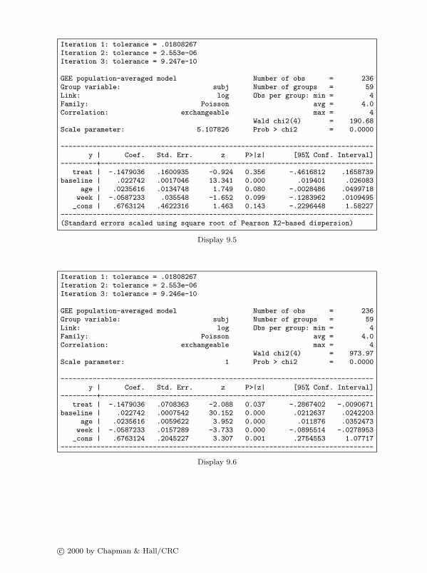
Iteration 1: tolerance = .01808267Iteration 2: tolerance = 2.553e-06Iteration 3: tolerance = 9.247e-10

GEE population-averaged model Number of obs = 236Group variable: subj Number of groups = 59Link: log Obs per group: min = 4Family: Poisson avg = 4.0Correlation: exchangeable max = 4


------------------------------------------------------------------------------y | Coef. Std. Err. z P>|z| [95% Conf. Interval]

---------+--------------------------------------------------------------------treat | -.1479036 .1600935 -0.924 0.356 -.4616812 .1658739

baseline | .022742 .0017046 13.341 0.000 .019401 .026083age | .0235616 .0134748 1.749 0.080 -.0028486 .0499718

week | -.0587233 .035548 -1.652 0.099 -.1283962 .0109495_cons | .6763124 .4622316 1.463 0.143 -.2296448 1.58227


Display 9.5



Wald chi2(4) = 973.97Scale parameter: 1 Prob > chi2 = 0.0000


---------+--------------------------------------------------------------------treat | -.1479036 .0708363 -2.088 0.037 -.2867402 -.0090671

baseline | .022742 .0007542 30.152 0.000 .0212637 .0242203age | .0235616 .0059622 3.952 0.000 .011876 .0352473

week | -.0587233 .0157289 -3.733 0.000 -.0895514 -.0278953_cons | .6763124 .2045227 3.307 0.001 .2754553 1.07717

------------------------------------------------------------------------------

Display 9.6


xtgee y treat baseline age week, corr(exc) family(pois) robust



Wald chi2(4) = 603.44Scale parameter: 1 Prob > chi2 = 0.0000

(standard errors adjusted for clustering on subj)------------------------------------------------------------------------------

| Semi-robusty | Coef. Std. Err. z P>|z| [95% Conf. Interval]

---------+--------------------------------------------------------------------treat | -.1479036 .1701506 -0.869 0.385 -.4813928 .1855855

baseline | .022742 .0012542 18.133 0.000 .0202839 .0252001age | .0235616 .0119013 1.980 0.048 .0002355 .0468877

week | -.0587233 .035298 -1.664 0.096 -.1279062 .0104595_cons | .6763124 .3570204 1.894 0.058 -.0234346 1.376059

------------------------------------------------------------------------------

Display 9.7

The results of the robust regression in Display 9.7 are remarkably similarto those of the overdispersed Poisson model, indicating that the latter is areasonable model for the data.

The estimated coefficient of treat describes the difference in the log ofthe average seizure counts between the placebo and progabide treated groups.The negative value indicates that the treatment is more effective than theplacebo in controlling the seizure rate although this is not significant. Theexponentiated coefficient gives an incidence rate ratio; here it represents theratio of average seizure rates, measured as the number of seizures per two-weekperiod, for the treated patients compared to that among the control patients.The exponentiated coefficient and the corresponding confidence interval canbe obtained directly using the eform option in xtgee:

xtgee y treat baseline age week, corr(exc) /**/ scale(x2) family(pois) eform

The results in Display 9.8 indicate that there is a 14% reduction in theincidence rate of epileptic seizures in the treated group compared with thecontrol group. According to the confidence interval, the reduction could be aslow as 37% or there could be a much as an 18% increase.





------------------------------------------------------------------------------y | IRR Std. Err. z P>|z| [95% Conf. Interval]

---------+--------------------------------------------------------------------treat | .8625142 .1380829 -0.924 0.356 .6302232 1.180424

baseline | 1.023003 .0017438 13.341 0.000 1.01959 1.026426age | 1.023841 .0137961 1.749 0.080 .9971555 1.051241

week | .9429676 .0335206 -1.652 0.099 .8795048 1.01101------------------------------------------------------------------------------(Standard errors scaled using square root of Pearson X2-based dispersion)

Display 9.8

When these data were analysed by Thall and Vail (1990), a possible interac-tion between baseline seizure count and treatment group was allowed for. Sucha model is easily fitted using the following instructions:

gen blint = treat*baselinextgee y treat baseline age week blint, /*

*/corr(exc) scale(x2) family(pois) eform

There is no evidence of an interaction in Display 9.9. Other correlation struc-tures might be explored for these data (see Exercises).

We now look at the standardized Pearson residuals of the previous modelseparately for each week, as an informal method for finding outliers (see equa-tion (7.9)). This can be done using the predict command to obtain estimatedcounts and computing the standardized Pearson residuals as follows:

quietly xtgee y treat baseline age week, corr(exc) /**/ family(pois) scale(x2)

predict pred, xbreplace pred = exp(pred)gen pres = (y-pred)/sqrt(pred)gen stpres = pres/sqrt(e(chi2_dis))sort weekgraph stpres, box s([subj]) by(week) ylab

The resulting graph is shown in Figure 9.3


Iteration 1: tolerance = .01714003Iteration 2: tolerance = .00001041Iteration 3: tolerance = 1.088e-08



------------------------------------------------------------------------------y | IRR Std. Err. z P>|z| [95% Conf. Interval]

---------+--------------------------------------------------------------------treat | .7735759 .1991683 -0.997 0.319 .4670343 1.281318

baseline | 1.021598 .0031501 6.930 0.000 1.015443 1.027791age | 1.025588 .0142413 1.820 0.069 .9980523 1.053884

week | .9429676 .0336645 -1.645 0.100 .8792419 1.011312blint | 1.001998 .003713 0.539 0.590 .994747 1.009302


Display 9.9

Figure 9.3 Standardized Pearson Residuals.


Here subject 25 is shown to be an outlier in week 3. In Figure 9.1 it isapparent that this is due to a large increase in the log of the seizure counts atweek 3.

9.4 Exercises

1. For the depression data, run the random effects model using different esti-mation methods available for xtreg. (See the Stata Reference Manual under‘xtreg’ for the interpretation of the fe and be options.)

2. Compare the result of the above with the result of running ordinary linearregression with standard errors corrected for the within-subject correlationusing

(a) the option, robust, cluster(subj), see help for regress, and(b) bootstrapping, by sampling subjects with replacement, not observations.

This may be achieved using the bs command, together with the optioncluster(subj).

3. Explore other possible correlational structures for the seizure data in thecontext of a Poisson model. Examine the robust standard errors in eachcase.

4. Investigate what Poisson models are most suitable when subject 25 is ex-cluded from the analysis.

5. Repeat the analysis treating the baseline measure (divided by four) as an-other response variable and replacing the variable week by a simple indicatorvariable, post, which is 0 at baseline and 1 subsequently. Is there a signifi-cant treatment effect, now represented by the interaction between post andtreat?


CHAPTER 10

Some Epidemiology


This chapter illustrates a number of different problems in epidemiology usingfour datasets that are presented in the form of cross-tabulations in Table 10.1.The first table (a) is taken from Clayton and Hills (1993). The data result froma cohort study which was carried out to investigate the relationship betweenenergy intake and ischaemic heart disease (IHD). Low energy intake indicateslack of physical exercise and is therefore considered a risk factor. The tablegives frequencies of IHD by ten year age-band and exposure to a high or lowcalory diet. The total person-years of observation are also given for each cell.

The second dataset (b) is the result of a case-control study investigatingwhether keeping a pet bird is a risk factor for lung cancer. This dataset isgiven in Hand et al. (1994).

The last two datasets (c) and (d) are from matched case control studies.In dataset (c), cases of endomitral cancer were matched on age, race, date ofadmission, and hospital of admission to a suitable control not suffering fromcancer. Past exposure to conjugated estrogens was determined. The datasetis described in Everitt (1994). The last set of data, described in Clayton andHills (1993), arise from a case-control study of breast cancer screening. Womenwho had died of breast cancer were matched with three control women. Thescreening history of the subjects in each matched case-control set was assessedover the period up to the time of diagnosis of the case.

10.2 Introduction to Epidemiology

Epidemiology is the study of diseases in populations, in particular the search forcauses of disease. For ethical reasons, subjects cannot be randomised to possiblerisk factors in order to establish whether these are associated with an increasein the incidence of disease. Instead, epidemiology is based on observationalstudies, the most important types being cohort studies and case-control studies.We will give a very brief description of the design and analysis of these twotypes of studies, following closely the explanations and notation given in theexcellent book, Statistical Models in Epidemiology by Clayton and Hills (1993)

In a cohort study, a group of subjects free of the disease is followed up and thepresence of risk factors as well as the occurrence of the disease of interest are


Table 10.1 Simple tables in epidemiology (a) number of IHD cases and person-years of observation by age and exposure to low energy diet; (b) The number of lungcancer cases and controls who keep a pet bird; (c) frequency of exposure tooral conjugated estrogens among cases of endomitral cancer and their matchedcontrols; (d) Screening history in subjects who died of breast cancer and 3matched controls. (Tables (a) and (d) taken from Clayton and Hills (1993)with permission of their publisher, Oxford University Press.)

(a) Cohort Study

Exposed Unexposed< 2750 kcal ≥ 2750 kcal

Age Cases Pers-yrs Cases Pers-yrs

40-49 2 311.9 4 607.950-59 12 878.1 5 1272.160-69 14 667.5 8 888.9

(b) Case-Control Study

Kept pet birds Cases Controls

yes 98 101no 141 328Total 239 429

(c) 1:1 Matched Case-Control Study

Controls

+ - TotalCases + 12 43 55

- 7 121 128Total 19 164 183

(d) 1:3 Matched Case-Control Study

Number ofcontrols screened

Status of the case 0 1 2 3

Screened 1 4 3 1Unscreened 11 10 12 4

recorded. This design is illustrated in Figure 10.1. An example of a cohort studyis the study described in the previous section where subjects were followed up inorder to monitor the occurrence of ischaemic heart disease in two risk groups,those with high and low energy intake, giving the results in Table 10.1 (a).The incidence rate λ (of the disease) may be estimated by the number of newcases of the disease D during a time interval divided by the person-time ofobservation Y , the sum of all subjects’ periods of observation during the timeinterval:

λ =D

Y. (10.1)

This is the maximum likelihood estimator of λ assuming that D follows a Pois-son distribution (independent events occurring at a constant probability ratein continuous time) with mean λY . The most important quantity of interest ina cohort study is the incidence rate ratio (or relative risk) between subgroupsof subjects defined by their exposure to the risk factor. This may be estimatedby

θ =D1/Y1

D0/Y0(10.2)


Cohortfree ofdisease2000

100 withdisease

1900 withoutdisease

✘✘✘✘✘✘✘✘✘✘✘✘✘✘✘✘✘✘✘✿

�

Now ✲ Future

Figure 10.1 Cohort Study.

where the subscripts 1 and 0 denote exposed and unexposed groups, respec-tively. This estimator may be derived by maximizing the conditional likelihoodthat there were D1 cases in the exposed group conditional on there being atotal of D = D0 + D1 cases. Since this conditional likelihood for θ is a truelikelihood based on the binomial distribution, exact confidence intervals maybe obtained. However, a potential problem in estimating this rate ratio is con-founding arising from systematic differences in prognostic factors between thegroups. This problem can be dealt with by dividing the cohort into groups orstrata according to such prognostic factors and assuming that the rate ratio forexposed and unexposed subjects is the same in each stratum. If there are Dt

cases and Y t person-years of observation in stratum t, then the common rateratio may be estimated using the method of Mantel and Haenszel as follows

θ =∑

t Dt1Y

t0 /Y

t∑t D

t0Y

t1 /Y

t. (10.3)

Note that the strata might not correspond to groups of subjects. For example,if the confounder is age, subjects who cross from one age-band into the nextduring the study, contribute parts of their periods of observation to differentstrata. This is how Table 10.1(a) was constructed. Another way of controllingfor confounding variables is to use Poisson regression to model the numberof failures. If a log link is used, the expected number of failures can be madeproportional to the person-years of observation by adding the log of the person-years of observation to the linear predictor as an offset (a term that is addedto the linear predictor without estimating a regression coefficient for it), giving

log(D) = log(Y ) + βT x. (10.4)


Exponentiating the equation gives

D = Y exp(βT x) (10.5)

as required.If the incidence rate of a disease is small, a cohort study requires a large

number of person-years of observation making it very expensive. A more fea-sible type of study in this situation is a case-control study in which cases ofthe disease of interest are compared with non-cases, called controls, with re-spect to exposure to possible risk factors in the past. A diagram illustratingthe basic idea of case-control studies is shown in Figure 10.2. The assumption

Population, 20000

Now

Past✻

Noncases19000

sample 0.53%

100 Controls

Exposed Nonexposed

��

��✒

❅❅

❅❅

Cases1000

sample 10%

100 Cases

Exposed Nonexposed

��

��✒

❅❅

❅❅

Figure 10.2 Case-Contr ol Study.

here is that the probability of selection into the study is independent of theexposures of interest. The data in Table 10.1(b) derive from a case-controlstudy in which cases with lung cancer and healthy controls were interviewedto ascertain whether or not they had been “exposed” to a pet bird.

Let D and H be the number of cases and controls respectively and let thesubscripts 0 and 1 denote “unexposed” and “exposed”. Since the proportion ofcases was determined by the design, it is not possible to estimate the relativerisk of disease between exposed and nonexposed subjects. However, the oddsof exposure in the cases or controls may be estimated and the ratio of theseodds

D1/D0

H1/H0=

D1/H1

D0/H0(10.6)

is equal to the odds ratio of being a case in the exposed group compared withthe unexposed group. If we model the (log) odds of being a case using logisticregression with the exposure as an explanatory variable, then the coefficientof the exposure variable is an estimate of the true log odds ratio even though


the estimate of the odds itself (reflected by the constant) only reflects theproportion of cases in the study. Logistic regression may therefore be used tocontrol for confounding variables.

A major difficulty with case-control studies is to find suitable controls whoare similar enough to the cases (so that differences in exposure can resonablybe assumed to be due their association with the disease) without being over-matched, which can result in very similar exposure patterns. The problem offinding cases who are similar enough is often addressed by matching cases in-dividually to controls according to important variables such as age and sex.Examples of such matched case-control studies are given in Table 10.1(b) and(c). In the screening study, matching had the following additional advantagenoted in Clayton and Hill (1993). The screening history of controls could bedetermined by considering only the period up to the diagnosis of the case, en-suring that cases did not have a decreased opportunity for screening becausethey would not have been screened after their diagnosis. The statistical analysishas to take account of the matching. Two methods of analysis are McNemar’stest in the case of two by two tables and conditional logistic regression in thecase of several controls per case and/or several explanatory variables.

Since the case-control sets have been matched on variables that are believedto be associated with disease status, the sets can be thought of as strata withsubjects in one stratum having higher or lower odds of being a case than thosein another after controlling for the exposures. A logistic regression model wouldhave to accommodate these differences by including a parameter ωc for eachcase-control set so that the log odds of being a case for subject i in case-controlset c would be

log(ωci) = log(ωc) + βT xi. (10.7)However, this would result in too many parameters to be estimated. Further-more, the parameters ωc are of no interest to us. In conditional logistic regres-sion, these nuisance parameters are eliminated as follows. In a 1:1 matchedcase-control study, ignoring the fact that each set has one case, the probabilitythat subject 1 in the set is a case and subject 2 is a noncase is

Pr(1) =ωc1

1 + ωc1× 1

1 + ωc2(10.8)

and the probability that subject 1 is a noncase and subject 2 is a case is

Pr(2) =1

1 + ωc1× ωc2

1 + ωc2. (10.9)

However, conditional on there being one case in a set, the probability of subject1 being the case is simply

Pr(1)Pr(1) + Pr(2)

= ωc1/(ωc1 + ωc2) =exp(βT x1)

exp(βT x1) + exp(βT x2)(10.10)

since ωc cancels out, see equation (10.7). The expression on the right-hand


side of equation (10.10) is the contribution of a single case-control set to theconditional likelihood of the sample. Similarly, it can be shown that if there arek controls per case and the subjects within each case-control set are labelled 1for the case and 2 to k + 1 for the controls then the log-likelihood becomes

∑c

log

(exp(βT x1)∑k+1

i=2 exp(βT xi)

). (10.11)


There is a collection of instructions in Stata, the epitab commands, that maybe used to analyse small tables in epidemiology. These commands either refer tovariables in an existing dataset or can they take cell counts as arguments (i.e.,there are immediate commands, see Chapter 1).

The first dataset (a) is given in a file as tabulated and may be read using

infile str5 age num0 py0 num1 py1 using ihd.dat,cleargen agegr= nreshape long num py, i(agegr) j(exposed)

Ignoring age, the incidence rate ratio may be estimated using

ir num exposed py

| exposed || Exposed Unexposed | Total

-----------------+------------------------+----------num | 17 28 | 45py | 2769 1857 | 4626

-----------------+------------------------+----------| |

Incidence Rate | .0061394 .0150781 | .0097276| || Point estimate | [95% Conf. Interval]|------------------------+----------------------

Inc. rate diff. | -.0089387 | -.0152401 -.0026372Inc. rate ratio | .4071738 | .2090942 .7703146 (exact)Prev. frac. ex. | .5928262 | .2296854 .7909058 (exact)Prev. frac. pop | .3548499 |

+-----------------------------------------------(midp) Pr(k<=17) = 0.0016 (exact)(midp) 2*Pr(k<=17) = 0.0031 (exact)

The incidence rate ratio is estimated as 0.41 with a 95% confidence intervalfrom 0.21 to 0.77. The terms (exact) imply that that the confidence intervalsare exact (no approximation was used). Controlling for age using the epitabcommand

ir num exposed py, by(age)


age | IRR [95% Conf. Interval] M-H Weight-----------------+-------------------------------------------------

40-49 | 1.026316 .1470886 11.3452 1.321739 (exact)50-59 | .2876048 .0793725 .8770737 7.099535 (exact)60-69 | .4293749 .1560738 1.096694 7.993577 (exact)

-----------------+-------------------------------------------------Crude | .4071738 .2090942 .7703146 (exact)

M-H combined | .4161246 .2262261 .7654276-----------------+-------------------------------------------------Test for heterogeneity (M-H) chi2(2) = 1.57 Pr>chi2 = 0.4554

gives very similar estimates as shown in the row labelled “M-H combined” (theMantel Haentzel estimate). Another way of controlling for age is to carry outPoisson regression with the log of py as an offset. The offset may be specifiedusing the exposure(py) option:

poisson num exposed, exposure(py) irr

Iteration 0: log likelihood = -13.906416Iteration 1: log likelihood = -13.906416

Poisson regression Number of obs = 6LR chi2(1) = 8.89Prob > chi2 = 0.0029


------------------------------------------------------------------------------num | IRR Std. Err. z P>|z| [95% Conf. Interval]

---------+--------------------------------------------------------------------exposed | .4072982 .125232 -2.921 0.003 .2229428 .7441002

py | (exposure)------------------------------------------------------------------------------

showing that there is an incidence rate ratio of 0.41 with a 95% confidenceinterval from 0.22 to 0.74. Another way of achieving the same result is usingglm with the offset option which requires the logarithm of the person-yearsto be computed.

gen lpy=log(py)glm num exposed, fam(poisson) link(log) offset(lpy) eform

where the eform option is used to obtain exponentiated coefficients.We will analyze the case-control study using the “immediate” command cci.

The following notation is used for cci

Exposed Unexposed

Cases a bNoncases c d

where the quantities a, b, etc. in the table are used in alphabetical order, i.e.,

cci a b c d


(See help epitab for the arguments required for other immediate epitab com-mands.) The bird data may therefore be analyzed using the immediate com-mand for case-control studies, cci, as follows:

cci 98 141 101 328

Proportion| Exposed Unexposed | Total Exposed

-----------------+------------------------+----------------------Cases | 98 141 | 239 0.4100

Controls | 101 328 | 429 0.2354-----------------+------------------------+----------------------

Total | 199 469 | 668 0.2979| || Pt. Est. | [95% Conf. Interval]|------------------------+----------------------

Odds ratio | 2.257145 | 1.606121 3.172163 (Cornfield)Attr. frac. ex. | .5569624 | .3773821 .6847577 (Cornfield)Attr. frac. pop | .2283779 |

+-----------------------------------------------chi2(1) = 22.37 Pr>chi2 = 0.0000

There is therefore a significant association between keeping pet birds and de-veloping lung cancer. The word (Cornfield) is there to remind us that anapproximation, the Cornfield approximation, was used to estimate the confi-dence interval (see for example Rothman, 1986).

The matched case-control study with one control per case may be ana-lyzed using the immediate command mcci where the columns of the two-waycrosstabulation represent exposed and unexposed controls:

mcci 12 43 7 121

| Controls |Cases | Exposed Unexposed | Total-----------------+------------------------+----------

Exposed | 12 43 | 55Unexposed | 7 121 | 128

-----------------+------------------------+----------Total | 19 164 | 183

McNemar’s chi2(1) = 25.92 Pr>chi2 = 0.0000Exact McNemar significance probability = 0.0000

Proportion with factorCases .3005464Controls .1038251 [95% conf. interval]

--------- --------------------difference .1967213 .1210924 .2723502ratio 2.894737 1.885462 4.444269rel. diff. .2195122 .1448549 .2941695

odds ratio 6.142857 2.739803 16.18481 (exact)


suggesting an increased odds of endimetrial cancer in subjects exposed to oralconjugated estrogens.

The matched case-control study with three controls per case cannot be an-alyzed using epitab. Instead, we will use conditional logistic regression. Weneed to convert the data from the table shown in 10.1 (d) into the form re-quired for conditional logistic regression; that is, one observation per subject(including cases and controls); an indicator variable, cancer, for cases; anotherindicator variable, screen, for screening and a third variable, caseid, givingthe id for each case-control set of four women.

First, read the data and transpose them so that the columns in the trans-posed dataset have variable names ncases0 and ncases1. The rows in thisdataset correspond to different numbers of matched controls who have beenscreened, which will be called nconstr. Then reshape to long, generating anindicator, casescr for whether or not the case was screened:

infile v1-v4 using screen.dat,cleargen str8 _varname="ncases1" in 1replace _varname="ncases0" in 2xpose, cleargen nconscr=_n-1reshape long ncases, i(nconscr) j(casescr)list

nconscr casescr ncases1. 0 0 112. 0 1 13. 1 0 104. 1 1 45. 2 0 126. 2 1 37. 3 0 48. 3 1 1

The next step is to replicate each of the records ncases times so that we haveone record per case-control set. Then define the variable caseid and expandthe dataset four times in order to have one record per subject. The four subjectswithin each case-control are arbitrarily labelled 0 to 3 in the variable controlwhere 0 stands for “the case” and 1, 2 and 3 for the controls.

expand ncasessort casescr nconscrgen caseid=_nexpand 4sort caseidquietly by caseid: gen control=_n-1list in 1/8


nconscr casescr ncases caseid control1. 0 0 11 1 02. 0 0 11 1 13. 0 0 11 1 24. 0 0 11 1 35. 0 0 11 2 06. 0 0 11 2 17. 0 0 11 2 28. 0 0 11 2 3

Now screen, the indicator whether a subject was screened, is defined to bezero except for the cases who were screened and for as many controls as werescreened according to nconscr. The variable cancer is one for cases and zerootherwise.

gen screen=0replace screen=1 if control==0&casescr==1 /* the case */replace screen=1 if control==1&nconscr>0replace screen=1 if control==2&nconscr>1replace screen=1 if control==3&nconscr>2gen cancer=cond(control==0,1,0)

We can reproduce Table 10.1(d) by temporarily collapsing the data (usingpreserve and restore to revert back to the original data) as follows:

preservecollapse (sum) screen (mean) casescr , by(caseid)gen nconscr=screen-casescrtabulate casescr nconscrrestore

(mean) | nconscrcasescr | 0 1 2 3 | Total

-----------+--------------------------------------------+----------0 | 11 10 12 4 | 371 | 1 4 3 1 | 9

-----------+--------------------------------------------+----------Total | 12 14 15 5 | 46

And now we are ready to carry out conditional logistic regression:

clogit cancer screen, group(caseid) or


Iteration 0: Log Likelihood =-62.404527Iteration 1: Log Likelihood =-59.212727Iteration 2: Log Likelihood = -59.18163Iteration 3: Log Likelihood =-59.181616

Conditional (fixed-effects) logistic regression Number of obs = 184chi2(1) = 9.18Prob > chi2 = 0.0025


------------------------------------------------------------------------------cancer | Odds Ratio Std. Err. z P>|z| [95% Conf. Interval]

---------+--------------------------------------------------------------------screen | .2995581 .1278367 -2.825 0.005 .1297866 .6914043

------------------------------------------------------------------------------

Screening is therefore protective of death from breast cancer, reducing the oddsto a third (95% 0.13 to 0.69).

10.4 Exercises

1. Carry out conditional logistic regression to estimate the odds ratio for thedata in Table 10.1 (c). The data are given in the same form as in the tablein a file called estrogen.dat.

2. For the data ihd.dat, use the command iri to calculate the incidence rateratio for IHD without controlling for age.

3. Use Poisson regression to test whether the effect of exposure on incidenceof IHD differs significantly between age groups.

4. Repeat the analysis of exercise 5 in Chapter 9, using the raw seizure counts(without dividing the baseline count by 4) as dependent variables and thelog of the observation time (8 weeks for baseline and 2 weeks for all othercounts) as an offset.


CHAPTER 11

Survival Analysis: Retention of HeroinAddicts in Methadone Maintenance

Treatment


The “survival data” to be analysed in this chapter are the times that heroinaddicts remained in a clinic for methadone maintenance treatment. The dataare given in Table 11.1. Here the endpoint of interest is not death as the word“survival” suggests, but termination of treatment. Some subjects were still inthe clinic at the time these data were recorded and this is indicated by thevariable status, which is equal to one if the person departed and 0 other-wise. Possible explanatory variables for retention in treatment are maximummethadone dose and a prison record as well as which of two clinics the addictwas treated in. These variables are called dose, prison and clinic respec-tively. The data were first analyzed by Caplehorn and Bell (1991) and alsoappear in Hand et al. (1994).

Table 11.1: Data in heroin.dat

id clinic status time prison dose id clinic status time prison dose1 1 1 428 0 50 132 2 0 633 0 702 1 1 275 1 55 133 2 1 661 0 403 1 1 262 0 55 134 2 1 232 1 704 1 1 183 0 30 135 2 1 13 1 605 1 1 259 1 65 137 2 0 563 0 706 1 1 714 0 55 138 2 0 969 0 807 1 1 438 1 65 143 2 0 1052 0 808 1 0 796 1 60 144 2 0 944 1 809 1 1 892 0 50 145 2 0 881 0 80

10 1 1 393 1 65 146 2 1 190 1 5011 1 0 161 1 80 148 2 1 79 0 4012 1 1 836 1 60 149 2 0 884 1 5013 1 1 523 0 55 150 2 1 170 0 4014 1 1 612 0 70 153 2 1 286 0 4515 1 1 212 1 60 156 2 0 358 0 6016 1 1 399 1 60 158 2 0 326 1 6017 1 1 771 1 75 159 2 0 769 1 4018 1 1 514 1 80 160 2 1 161 0 4019 1 1 512 0 80 161 2 0 564 1 8021 1 1 624 1 80 162 2 1 268 1 7022 1 1 209 1 60 163 2 0 611 1 4023 1 1 341 1 60 164 2 1 322 0 5524 1 1 299 0 55 165 2 0 1076 1 8025 1 0 826 0 80 166 2 0 2 1 4026 1 1 262 1 65 168 2 0 788 0 70


Table 11.1: Data in heroin.dat (continued)

27 1 0 566 1 45 169 2 0 575 0 8028 1 1 368 1 55 170 2 1 109 1 7030 1 1 302 1 50 171 2 0 730 1 8031 1 0 602 0 60 172 2 0 790 0 9032 1 1 652 0 80 173 2 0 456 1 7033 1 1 293 0 65 175 2 1 231 1 6034 1 0 564 0 60 176 2 1 143 1 7036 1 1 394 1 55 177 2 0 86 1 4037 1 1 755 1 65 178 2 0 1021 0 8038 1 1 591 0 55 179 2 0 684 1 8039 1 0 787 0 80 180 2 1 878 1 6040 1 1 739 0 60 181 2 1 216 0 10041 1 1 550 1 60 182 2 0 808 0 6042 1 1 837 0 60 183 2 1 268 1 4043 1 1 612 0 65 184 2 0 222 0 4044 1 0 581 0 70 186 2 0 683 0 10045 1 1 523 0 60 187 2 0 496 0 4046 1 1 504 1 60 188 2 1 389 0 5548 1 1 785 1 80 189 1 1 126 1 7549 1 1 774 1 65 190 1 1 17 1 4050 1 1 560 0 65 192 1 1 350 0 6051 1 1 160 0 35 193 2 0 531 1 6552 1 1 482 0 30 194 1 0 317 1 5053 1 1 518 0 65 195 1 0 461 1 7554 1 1 683 0 50 196 1 1 37 0 6055 1 1 147 0 65 197 1 1 167 1 5557 1 1 563 1 70 198 1 1 358 0 4558 1 1 646 1 60 199 1 1 49 0 6059 1 1 899 0 60 200 1 1 457 1 4060 1 1 857 0 60 201 1 1 127 0 2061 1 1 180 1 70 202 1 1 7 1 4062 1 1 452 0 60 203 1 1 29 1 6063 1 1 760 0 60 204 1 1 62 0 4064 1 1 496 0 65 205 1 0 150 1 6065 1 1 258 1 40 206 1 1 223 1 4066 1 1 181 1 60 207 1 0 129 1 4067 1 1 386 0 60 208 1 0 204 1 6568 1 0 439 0 80 209 1 1 129 1 5069 1 0 563 0 75 210 1 1 581 0 6570 1 1 337 0 65 211 1 1 176 0 5571 1 0 613 1 60 212 1 1 30 0 6072 1 1 192 1 80 213 1 1 41 0 6073 1 0 405 0 80 214 1 0 543 0 4074 1 1 667 0 50 215 1 0 210 1 5075 1 0 905 0 80 216 1 1 193 1 7076 1 1 247 0 70 217 1 1 434 0 5577 1 1 821 0 80 218 1 1 367 0 4578 1 1 821 1 75 219 1 1 348 1 6079 1 0 517 0 45 220 1 0 28 0 5080 1 0 346 1 60 221 1 0 337 0 4081 1 1 294 0 65 222 1 0 175 1 6082 1 1 244 1 60 223 2 1 149 1 8083 1 1 95 1 60 224 1 1 546 1 5084 1 1 376 1 55 225 1 1 84 0 4585 1 1 212 0 40 226 1 0 283 1 8086 1 1 96 0 70 227 1 1 533 0 5587 1 1 532 0 80 228 1 1 207 1 5088 1 1 522 1 70 229 1 1 216 0 5089 1 1 679 0 35 230 1 0 28 0 5090 1 0 408 0 50 231 1 1 67 1 5091 1 0 840 0 80 232 1 0 62 1 6092 1 0 148 1 65 233 1 0 111 0 55


Table 11.1: Data in heroin.dat (continued)

93 1 1 168 0 65 234 1 1 257 1 6094 1 1 489 0 80 235 1 1 136 1 5595 1 0 541 0 80 236 1 0 342 0 6096 1 1 205 0 50 237 2 1 41 0 4097 1 0 475 1 75 238 2 0 531 1 4598 1 1 237 0 45 239 1 0 98 0 4099 1 1 517 0 70 240 1 1 145 1 55

100 1 1 749 0 70 241 1 1 50 0 50101 1 1 150 1 80 242 1 0 53 0 50102 1 1 465 0 65 243 1 0 103 1 50103 2 1 708 1 60 244 1 0 2 1 60104 2 0 713 0 50 245 1 1 157 1 60105 2 0 146 0 50 246 1 1 75 1 55106 2 1 450 0 55 247 1 1 19 1 40109 2 0 555 0 80 248 1 1 35 0 60110 2 1 460 0 50 249 2 0 394 1 80111 2 0 53 1 60 250 1 1 117 0 40113 2 1 122 1 60 251 1 1 175 1 60114 2 1 35 1 40 252 1 1 180 1 60118 2 0 532 0 70 253 1 1 314 0 70119 2 0 684 0 65 254 1 0 480 0 50120 2 0 769 1 70 255 1 0 325 1 60121 2 0 591 0 70 256 2 1 280 0 90122 2 0 769 1 40 257 1 1 204 0 50123 2 0 609 1 100 258 2 1 366 0 55124 2 0 932 1 80 259 2 0 531 1 50125 2 0 932 1 80 260 1 1 59 1 45126 2 0 587 0 110 261 1 1 33 1 60127 2 1 26 0 40 262 2 1 540 0 80128 2 0 72 1 40 263 2 0 551 0 65129 2 0 641 0 70 264 1 1 90 0 40131 2 0 367 0 70 266 1 1 47 0 45

The main reason why survival data require special methods of analysis is be-cause they often contain right censored observations; that is, observations forwhich the endpoint of interest has not occurred during the period of observa-tion; all that is known about the true survival time is that it exceeds the periodof observation. Even if there are no censored observations, survival times tendto have positively skewed distributions that can be difficult to model.

11.2 Describing survival times and Cox’s regression model

The survival time T may be regarded as a random variable with a probabilitydistribution F (t) and probability density function f(t). Then an obvious func-tion of interest is the probability of surviving to time t or beyond, the survivorfunction or survival curve S(t), which is given by

S(t) = P (T ≥ t) = 1 − F (t). (11.1)

A further function which is of interest for survival data is the hazard function;this represents the instantaneous failure rate; that is, the probability that anindividual expriences the event of interest at a time point given that the event


has not yet occurred. It can be shown that the hazard function is given by

h(t) =f(t)S(t)

, (11.2)

the instantaneous probability of failure at time t divided by the probability ofsurviving up to time t. Note that the hazard function is just the incidence ratediscussed in Chapter 10. It follows from (11.1) and (11.2) that

−d log(S(t))dt

= h(t) (11.3)

so thatS(t) = exp(−H(t)) (11.4)

where H(t) is the integrated hazard function, also known as the cumulativehazard function.

11.2.1 Cox’s Regression

Cox’s regression is a semi-parametric approach to survival analysis. The methoddoes not require the probability distribution F (t) to be specified; however, un-like most nonparametric methods, Cox’s regression does use regression param-eters in the same way as generalized linear models. The model can be writtenas

h(t) = h0(t) exp(βT x) (11.5)so that the hazard functions of any two individuals are assumed to be constantmultiples of each other, the multiple being exp(βT (xi − xj)), the hazard ratioor incidence rate ratio. The assumption of a constant hazard ratio is calledthe proportional hazards assumption. The set of parameters h0(t), called thebaseline hazard function, can be thought of as nuisance parameters whosepurpose is merely to control the parameters of interest β for any changes inthe hazard over time. The parameters β are estimated by maximizing thepartial log likelihood given by

∑f

log

(exp(βT xf )∑

i∈r(f) exp(βT xi)

)(11.6)

where the first summation is over all failures f and the second summation isover all subjects r(f) still alive (and therefore “at risk”) at the time of failure.It can be shown that this log-likelihood is a log profile likelihood (i.e., thelog of the likelihood in which the nuisance parameters have been replaced byfunctions of β which maximise the likelihood for fixed β). Note also that thelikelihood in equation (11.6) is equivalent to the likelihood for matched case-control studies described in Chapter 10 if the subjects at risk at the time ofa failure (the risk set) are regarded as controls matched to the case failing atthat point in time (see Clayton and Hills, 1993).


The baseline hazards may be estimated by maximizing the full log likelihoodwith the regression parameters evaluated at their estimated values. These haz-ards are nonzero only when a failure occurs. Integrating the hazard functiongives the cumulative hazard function

H(t) = H0(t) exp(βT x) (11.7)

where H0(t) is the integral of h0(t). The survival curve may be obtained fromH(t) using equation (11.4).

It follows from equation (11.4), that the survival curve for a Cox model isgiven by

S(t) = S0(t)exp(βTx) (11.8)

The log of the cumulative hazard function predicted by the Cox model isgiven by

log(H(t)) = log H0(t) + βT x, (11.9)

so that the log cumulative hazard functions of any two subjects i and j areparallel with constant difference given by βT (xi − xj).

If the subjects fall into different groups and we are not sure whether wecan make the assumption that the group’s hazard functions are proportionalto each other, we can estimate separate log cumulative hazard functions forthe groups using a stratified Cox model. These curves may then be plotted toassess whether they are sufficiently parallel. For a stratified Cox model, thepartial likelihood has the same form as in equation (11.6) except that the riskset for a failure is now confined to subjects in the same stratum.

Survival analysis is described in detail in Collett (1994) and in Clayton andHills (1993).


The data are available as an ASCII file called heroin.dat on the disk accom-panying Hand et al. (1994). Since the data are stored in a two-column formatwith the set of variables repeated twice in each row, as shown in Table 11.1,we have to use reshape to bring the data into the usual form:

infile id1 clinic1 status1 time1 prison1 dose1 /**/ id2 clinic2 status2 time2 prison2 dose2 /**/ using heroin.dat

gen row=_nreshape long id clinic status time prison dose, /*

*/ i(row) j(col)drop row col

Before fitting any survival time models, we declare the data as being of theform “st” (for survival time) using the stset command


stset time, failure(status)

failure event: status ~= 0 & status ~= .obs. time interval: (0, time]exit on or before: failure

------------------------------------------------------------------------------238 total obs.

0 exclusions------------------------------------------------------------------------------

238 obs. remaining, representing150 failures in single record/single failure data

95812 total analysis time at risk, at risk from t = 0earliest observed entry t = 0

last observed exit t = 1076

and look at a summary of the data using

stsum

failure _d: statusanalysis time _t: time

| incidence no. of |------ Survival time -----|| time at risk rate subjects 25% 50% 75%

---------+---------------------------------------------------------------------total | 95812 .0015656 238 212 504 821

There are therefore 238 subjects with a median survival time of 504 days. Ifthe incidence rate (i.e. the hazard function) could be assumed to be constant,it would be estimated as 0.0016 per day which corresponds to 0.57 per year.

The data come from two different clinics and it is likely that these clinics havedifferent hazard functions which may well not be parallel. A Cox regressionmodel with clinics as strata and the other two variables, dose and prison asexplanatory variables is fitted using the stcox command with the strata()option:

stcox dose prison, strata(clinic)

giving the output shown in Display 11.1. Therefore, subjects with a prison his-tory are 47.5% more likely to drop out at any given time (given that they re-mained until that time) than those without a prison history. For every increasein methadone dose by one unit (1mg), the hazard is multiplied by 0.965. Thiscoefficient is very close to one, but this may be because one unit of methadonedose is not a large quantity. Even if we know little about methadone mainte-nance treatment, we can assess how much one unit of methadone dose is byfinding the sample standard deviation:

summarize dose


dose | 238 60.39916 14.45013 20 110



Iteration 0: log likelihood = -614.68365Iteration 1: log likelihood = -597.73516Iteration 2: log likelihood = -597.714Refining estimates:Iteration 0: log likelihood = -597.714

Stratified Cox regr. -- Breslow method for ties

No. of subjects = 238 Number of obs = 238No. of failures = 150Time at risk = 95812

LR chi2(2) = 33.94Log likelihood = -597.714 Prob > chi2 = 0.0000

------------------------------------------------------------------------------_t |_d | Haz. Ratio Std. Err. z P>|z| [95% Conf. Interval]

---------+--------------------------------------------------------------------dose | .9654655 .0062418 -5.436 0.000 .953309 .977777

prison | 1.475192 .2491827 2.302 0.021 1.059418 2.054138------------------------------------------------------------------------------

Stratified by clinic

Display 11.1

indicating that a unit is not much at all; subjects often differ from each otherby 10 to 15 units. To find the hazard ratio of two subjects differing by onestandard deviation, we need to raise the hazard ratio to the power of onestandard deviation, giving 0.965465514.45013 = 0.60179167. We can obtain thesame result (with greater precision) using the stored macros b[dose] for thelog hazard ratio and r(Var) for the variance,

disp exp( b[dose]*sqrt(r(Var)))

.60178874

In the above calculation we simply rescaled the regression coefficient beforetaking the exponential. To obtain this hazard ratio in the Cox regression,standardize dose to have unit standard deviation. In the command below wealso standardize to mean zero although this will make no difference to theestimated coefficients (except the constant):

egen zdose=std(dose)

we repeat the Cox regresion with the option bases(s) which results in thebaseline survival function S0(t) being estimated and stored in s:

stcox zdose prison, strata(clinic) bases(s)



Iteration 0: log likelihood = -614.68365Iteration 1: log likelihood = -597.73516Iteration 2: log likelihood = -597.714Refining estimates:Iteration 0: log likelihood = -597.714





---------+--------------------------------------------------------------------zdose | .6017887 .0562195 -5.436 0.000 .5010998 .7227097

prison | 1.475192 .2491827 2.302 0.021 1.059418 2.054138------------------------------------------------------------------------------


The coefficient of zdose is identical to that calculated previously and maynow be interpreted as indicating a decrease of the hazard by 40% when themethadone dose increases by one standard deviation.

One question to investigate is whether the clinics need to be treated as strataor whether the hazard functions are in fact proportional. We may do this byplotting the log cumulative hazard function for the two clinics and visually as-sessing whether these curves are approximately parallel. The variables requiredfor the graph are obtained as follows:

gen lh1=log(-log(s)) if clinic==1gen lh2=log(-log(s)) if clinic==2

To find out where the two curves end so that we can label them at those point,we sort the data by time within clinic and list the last observation within clinic

sort clinic timeby clinic: list clinic status time lh1 lh2 if n== N

-> clinic= 1clinic status time lh1 lh2

163. 1 0 905 1.477235 .

-> clinic= 2clinic status time lh1 lh2

238. 2 0 1076 . -.4802778


showing that the curves end at times 905 and 1075, respectively, with corre-sponding values on the vertical axis of 1.48 and −0.48. In order to plot labels“clin1” and “clin2” near these points, we can define new variables pos1 andpos2 equal to the y-positions for the two labels when time is equal to therequired positions on the time-axis and equal to missing for all other valuesof time. We also need two string variables, lab1 and lab2 to hold the corre-sponding labels, to be applied at the points in pos1 and pos2 using the s()option.

gen pos1=1.48+0.2 if time==905gen str5 lab1="clin1"gen pos2=-0.48+0.2 if time==1076gen str5 lab2="clin2"

The graph is produced using

graph lh1 lh2 pos1 pos2 time, sort s(ii[lab1][lab2]) c(JJ..) /**/ xlabel ylabel pen(6311) psize(130) t1(" ") gap(3) /**/ l1("Log of cumulative hazard")

Here, the option connect(J), abbreviated c(J), causes points to be connectedusing a step function and pen(6311) was used to control the colours (and thick-nesses) of the lines and plotting symbols, mainly to have the labels appear inthe same colour (pen=1) as the axes and titles. The resulting graph is shownin Figure 11.1. In these curves, the increment at each failure represents theestimated log of the hazards at that time. Clearly, the curves are not paralleland we will therefore continue treating the clinics as strata. Note that a quickerway of producing a similar graph would be to use the stphplot command asfollows:

stphplot, strata(clinic) xlabel ylabel adjust(zdose prison) /**/ zero gap(3) psize(130)

Here the adjust() option specifies the covariates to be used in the Cox regres-sion, and the zero option specifies that these covariates are to be evaluated atzero. As a result, minus the log of the baseline survival functions (stratified byclinics) are plotted agains the log of the survival time, see Figure 11.2.

11.3.1 Model presentation and diagnostics

Assuming the variables prison and zdose satisfy the proportional hazardsassumption (see Section 11.3.2), we now discuss how to present the model.

A good graph for presenting the results of a Cox regression is a graph ofthe survival curves fitted for groups of subjects when the continuous variablestake on their mean values. Such a graph may be produced by first generating


Figure 11.1 Log of minus the log of the survival functions for the two clinics estimatedby stratified Cox regression.

variables surv1 and surv2 to hold the fitted baseline survival curves for thetwo groups and then applying equation (11.8) to obtain the survival curves forparticular covariate values:

stcox zdose prison, strata(clinic) bases(s_strat)egen mdose=mean(zdose), by(clinic)gen surv1=s_strat^exp(_b[zdose]*mdose) if prison==0gen surv2=s_strat^exp(_b[zdose]*mdose+_b[prison]) if prison==1

Note that the survival functions represent the expected survival function for asubject having the clinic-specific mean dose. We now transform time to timein years and plot the survival curves separately for each clinic:

gen tt=time/365.25label variable tt "time in years"graph surv1 surv2 tt, sort c(JJ) s(..) by(clinic) t1(" ") /*

*/ xlabel ylabel(0.0,0.2,0.4,0.6,0.8,1.0)

resulting in two graphs displayed side by side at the top of the graphics windowseparated by a wide gap from a title at the bottom of the window. A better


Figure 11.2 Minus the log of minus the log of the survival functions for the two clinicsversus log survival time, estimated by stratified Cox regression.

looking figure can be produced by displaying separate graphs for the clinicsside by side where, the separate graphs are created using

graph surv1 surv2 tt if clinic==1 , sort c(JJ) s(..) gap(3) /**/ xlabel(0,1,2,3) ylabel(0.0,0.2,0.4,0.6,0.8,1.0) /**/ t1("clinic 1") l1("fraction remaining")

and similarly for clinic 2. The result is shown in Figure 11.3.According to Caplehorn and Bell (1991), the more rapid decline in the pro-

portion remaining in clinic 1 compared with clinic 2 may be due to the policyof clinic 1 to attempt to limit the duration of maintenance to two years.

It is probably a good idea to produce some residual plots, for example a graphof the deviance residuals against the linear predictor. In order for predict tobe able to compute the deviance residuals, we must first store the martingaleresiduals (see for example Collett, 1994) using stcox with the mgale() option:

stcox zdose prison, strata(clinic) mgale(mart)predict devr, deviancepredict xb, xbgraph devr xb, xlabel ylabel s([id]) gap(3) /*


Figure 11.3 Survival curves.

*/ l1("Deviance Residuals")

with the result shown in Figure 11.4. There appear to be no serious outliers.

Figure 11.4 Deviance residuals for survival analysis.

Another type of residual is a score residual, defined as the first derivative ofthe partial log likelihood function with respect to an explanatory variable. Thescore residual is large in absolute value if a case’s explanatory variable differssubstantially from the explanatory variables of subjects whose estimated risk


of failure is large at the case’s time of failure or censoring. Since our model hastwo explanatory variables, we can compute the score residuals for zdose andprison and store them in score1 and score2 using the command

drop s stratstcox zdose prison, strata(clinic) bases(s strat) esr(score*)

These residuals can be plotted against survival time using

label variable score1 "score residuals for zdose"graph score1 tt, s([id]) gap(3) xlabel ylabel

and similarly for score2. The resulting graphs are shown in Figures 11.5and 11.6. Subject 89 has a low value of zdose (-1.75) compared with othersubjects at risk of failure at such a late time. Subjects 8, 27, 12 and 71 leaverelatively late considering that they have a police record whereas other re-mainers at their time of leaving (or censoring) tend to have no police record.

Figure 11.5 Score residuals for zdose.


Figure 11.6 Score residuals for prison.

11.3.2 Cox’s regression with time-varying covariates

In order to determine whether the hazard functions for those with and withouta prison history are proportional, we could split the data into four strata byclinic and prison. However, as the strata get smaller, the estimated survivalfunctions become less precise (due to the risk sets in equation (11.6) becomingsmaller). Also, a similar method could not be used to check the proportionalhazard assumption for the continuous variable zdose. Another way of testingthe proportional hazards assumption of zdose, say, is to introduce a time-varying covariate equal to the interaction between the survival time variableand zdose. In order to estimate this model, the terms in equation (11.6) needto be evaluated using the values of the time-varying covariates at the timesof the failure. These values are not available in the present dataset since eachsubject is represented only once, at the time of their own failure. We thereforeneed to expand the dataset so that each subject’s record appears (at least)as many times as that subject contributes to a risk set in equation (11.6),with the time variable equal to the corresponding failure times. The simplestway to achieve this for discrete survival times is to represent each subject by tiobservations (where ti is subject i’s survival time) with the variable time equalto 1,2,· · ·,ti. The invented survival times are times beyond which the subject


survives, so the status variable fail, is set to zero for all invented times andequal to status for the original survival time. The following code is adaptedfrom the Stata FAQ by W. Gould (1999) (to look at the FAQ, do a search withkeyword equal to “time-varying”, click into url of the appropriate FAQ entry).

expand timesort idquietly by id: gen t = _ngen fail = 0quietly by id: replace fail = status if _n==_N

The same may be achieved with a more concise syntax:

stset time, failure(status) id(id)quietly summarize _t, meanonlystsplit cat, at(0(1)`r(max)´)

A problem with applying this code to our data is that our survival times aremeasured in days with a median survival of 504 days. Unless we are willingto round time, for example to integer number of months, we would have toreplicate the data by a factor of about 500! Therefore a more feasible methodis described in several stages.

Before we begin, we must make sure that we have enough memory allocatedto Stata to hold the increased dataset. The memory may be set to 3 mega-bytesusing

clearset memory 3m

(the data have to be read in again after this). If set memory does not work,add the /k3000 option to the command for running Stata, e.g.,

C:\Stata\wstata.exe /k3000

in the Target field of the Shortcut tab accessed by right-mouse clicking intothe Stata icon and selecting Properties. We will also need to define matricesand in order to ensure that we do not exceed the maximum matrix size, weincrease the limit to 300 using set matsize:

set matsize 300

The first step is to determine the sets of unique failure times for the two clinicsand store these in matrices t1 and t2 using the command mkmat:

sort clinic status timegen unft=0 /* indicator for unique failure times */quietly by clinic status time: replace unft=1 if _n==1&status==1


sort timemkmat time if (unft==1)&clinic==1,matrix(t1)sort timemkmat time if (unft==1)&clinic==2,matrix(t2)

We can look at the contents of t2 using

matrix list t2

with the result shown in Display 11.2. Note that t2 is a matrix although it

t2[27,1]time

r1 13r2 26r3 35r4 41r5 79r6 109r7 122r8 143r9 149

r10 161r11 170r12 190r13 216r14 231r15 232r16 268r17 280r18 286r19 322r20 366r21 389r22 450r23 460r24 540r25 661r26 708r27 878

Display 11.2

only holds a one-dimensional array of numbers. This is because there are novectors in Stata. The matrix is r × 1 where r can be found using the functionrowsof(t2). Elements of the matrix may be accessed using the expressiont2[3,1] for the third unique failure time in clinic2.

Next, determine num, the number of replicates required of each subject’srecord. Initially, num is set equal to the number of unique survival times ineach subject’s clinic, i.e. the number of rows of the corresponding matrix:

local nt1=rowsof(t1)


local nt2=rowsof(t2)gen num=cond(clinic==1,`nt1´,`nt2´)

However, the number of required replicates is just the number of uniquesurvival times which are less than the subject’s own survival time, time becausethe subject ceases to contribute to future risk sets once it has failed (or hasbeen censored). Therefore, reduce num until t1[num,1] is less than time forthe first time, implying that t1[num+1,1] is greater than time:

local i=1while ì´<=`nt1´

qui replace num=num-1 /**/ if clinic==1&time<=t1[`nt1´-ì´+1,1]

local i=ì´+1

local i=1while ì´<=`nt2´

qui replace num=num-1 /**/ if clinic==2&time<=t2[`nt2´-ì´+1,1]

local i=ì´+1

We need one extra record for each subject to hold their own survival time:

replace num=num+1

We are now ready to expand the dataset and fill in the unique survivaltimes for the first num-1 records of each subject, followed by the subject’s ownsurvival time in the last record. All except the last values of the new variablefail (for failure status) will be 0 (for censored) and the last value will be equalto the subject’s status at the time of their own failure or censoring:

compressdisp _Nexpand numdisp _N

sort id timequietly by id: gen t=cond(clinic==1,t1[_n,1],t2[_n,1])sort id tquietly by id: replace t=time if _n==_N

gen fail=0 /* indicator for failure */sort id tquietly by id: replace fail=status if _n==_N


The command compress was used before expand to ensure that the variablesare stored as compactly as possible before another 10990 observations werecreated. The data are now in a suitable form to perfom Cox regression withtime-varying covariates. We first verify that the data are equivalent to theoriginal form by repeating the simple Cox regression

stset t, failure(fail) id(id)stcox zdose prison, strata(clinic)

which gives the same result as before. We can now generate a time-varyingcovariate for zdose as follows:

gen tdose=zdose*(t-504)/365.25

where we have subtracted the median survival time so that the effect of theexplanatory variable zdose can be interpreted as the effect of zdose at themedian survival time. We have divided by 365.25 to see by how much theeffect of zdose changes between intervals of one year. We now fit the Coxregression, allowing the effect of zdose to vary with time:

stcox zdose tdose prison, strata(clinic)

In the output shown in Display 11.3, the estimated increase in the hazardratio for zdose is 15% per year. This small effect is not significant at the 5%level which is confirmed by carrying out the likelihood ratio test as follows:

lrtest, saving(0)quietly stcox zdose prison, strata(clinic)lrtest

Cox: likelihood-ratio test chi2(1) = 0.85Prob > chi2 = 0.3579

giving a very similar p-value as before and confirming that there is no evidencethat the effect of dose on the hazard varies with time. A similar test can becarried out for prison (see Exercise 5).

We can now return back to the original data, either by reading them againor by dropping all the newly created observations as follows:

sort id tquietly by id: drop if n< Nstset t, failure(fail)stcox zdose prison, strata(clinic) bases(s strat)

11.4 Exercises

1. In the original analysis of this data, Caplehorn and Bell (1991) judged thatthe hazards were approximately proportional for the first 450 days (see


failure _d: failanalysis time _t: t

id: id

Iteration 0: log likelihood = -614.68365Iteration 1: log likelihood = -597.32655Iteration 2: log likelihood = -597.29131Iteration 3: log likelihood = -597.29131Refining estimates:Iteration 0: log likelihood = -597.29131





---------+--------------------------------------------------------------------zdose | .6442974 .0767535 -3.690 0.000 .5101348 .8137442tdose | 1.147853 .1720104 0.920 0.357 .8557175 1.539722

prison | 1.481193 .249978 2.328 0.020 1.064036 2.061899------------------------------------------------------------------------------


Display 11.3

Figure 11.1). They therefore analyzed the data for this time period usingclinic as a covariate instead of stratifying by clinic. Repeat this analysis,using prison and dose as further covariates.

2. Following Caplehorn and Bell (1991), repeat the above analysis treatingdose as a categorical variable with three levels (< 60, 60 − 79, ≥ 80) andplot the predicted survival curves for the three dose categories when prisonand clinic take on one of their values.

3. Test for an interaction between clinic and the methadone dose using bothcontinuous and categorical scales for dose.

4. Create a “do-file” containing the commands given above to expand the datafor Cox regression with time-varying covariates.

5. Read and expand the data (using the “do-file”) and check the proportionalhazards assumption for prison using the same method we used for dose.


CHAPTER 12

Principal Components Analysis:Hearing Measurement using an

Audiometer


The data in Table 12.1 are adapted from those given in Jackson (1991), andrelate to hearing measurement with an instrument called an audiometer. Anindividual is exposed to a signal of a given frequency with an increasing inten-sity until the signal is perceived. The lowest intensity at which the signal isperceived is a measure of hearing loss, calibrated in units referred to as deci-bel loss in comparison to a reference standard for that particular instrument.Observations are obtained one ear at a time, for a number of frequencies. Inthis example the frequencies used were 500 Hz, 1000 Hz, 2000 Hz and 4000Hz. The limits of the instrument are -10 to 99 decibels. (A negative value doesnot imply better than average hearing; the audiometer had a calibration ‘zero’and these observations are in relation to that).

Table 12.1: Data in hear.dat (Taken from Jackson (1992) with per-mission of his publisher, John Wiley and Sons).

id l500 l1000 l2000 l4000 r500 r1000 r2000 r4000

1 0 5 10 15 0 5 5 152 -5 0 -10 0 0 5 5 153 -5 0 15 15 0 0 5 154 -5 0 -10 -10 -10 -5 -10 105 -5 -5 -10 10 0 -10 -10 506 5 5 5 -10 0 5 0 207 0 0 0 20 5 5 5 108 -10 -10 -10 -5 -10 -5 0 59 0 0 0 40 0 0 -10 10

10 -5 -5 -10 20 -10 -5 -10 1511 -10 -5 -5 5 5 0 -10 512 5 5 10 25 -5 -5 5 1513 0 0 -10 15 -10 -10 -10 1014 5 15 5 60 5 5 0 5015 5 0 5 15 5 -5 0 2516 -5 -5 5 30 5 5 5 25


Table 12.1: Data in hear.dat (Taken from Jackson (1992) with permissionof his publisher, John Wiley and Sons) (continued)

17 0 -10 0 20 0 -10 -10 2518 5 0 0 50 10 10 5 6519 -10 0 0 15 -10 -5 5 1520 -10 -10 -5 0 -10 -5 -5 521 -5 -5 -5 35 -5 -5 -10 2022 5 15 5 20 5 5 5 2523 -10 -10 -10 25 -5 -10 -10 2524 -10 0 5 15 -10 -5 5 2025 0 0 0 20 -5 -5 10 3026 -10 -5 0 15 0 0 0 1027 0 0 5 50 5 0 5 4028 -5 -5 -5 55 -5 5 10 7029 0 15 0 20 10 -5 0 1030 -10 -5 0 15 -5 0 10 2031 -10 -10 5 10 0 0 20 1032 -5 5 10 25 -5 0 5 1033 0 5 0 10 -10 0 0 034 -10 -10 -10 45 -10 -10 5 4535 -5 10 20 45 -5 10 35 6036 -5 -5 -5 30 -5 0 10 4037 -10 -5 -5 45 -10 -5 -5 5038 5 5 5 25 -5 -5 5 4039 -10 -10 -10 0 -10 -10 -10 540 10 20 15 10 25 20 10 2041 -10 -10 -10 20 -10 -10 0 542 5 5 -5 40 5 10 0 4543 -10 0 10 20 -10 0 15 1044 -10 -10 10 10 -10 -10 5 045 -5 -5 -10 35 -5 0 -10 5546 5 5 10 25 10 5 5 2047 5 0 10 70 -5 5 15 4048 5 10 0 15 5 10 0 3049 -5 -5 5 -10 -10 -5 0 2050 -5 0 10 55 -10 0 5 5051 -10 -10 -10 5 -10 -10 -5 052 5 10 20 25 0 5 15 053 -10 -10 50 25 -10 -10 -10 4054 5 10 0 -10 0 5 -5 1555 15 20 10 60 20 20 0 2556 -10 -10 -10 5 -10 -10 -5 -1057 -5 -5 -10 30 0 -5 -10 1558 -5 -5 0 5 -5 -5 0 1059 -5 5 5 40 0 0 0 1060 5 10 30 20 5 5 20 6061 5 5 0 10 -5 5 0 10


Table 12.1: Data in hear.dat (Taken from Jackson (1992) with permissionof his publisher, John Wiley and Sons) (continued)

62 0 5 10 35 0 0 5 2063 -10 -10 -10 0 -5 0 -5 064 -10 -5 -5 20 -10 -10 -5 565 5 10 0 25 5 5 0 1566 -10 0 5 60 -10 -5 0 6567 5 10 40 55 0 5 30 4068 -5 -10 -10 20 -5 -10 -10 1569 -5 -5 -5 20 -5 0 0 070 -5 -5 -5 5 -5 0 0 571 0 10 40 60 -5 0 25 5072 -5 -5 -5 -5 -5 -5 -5 573 0 5 45 50 0 10 15 5074 -5 -5 10 25 -10 -5 25 6075 0 -10 0 60 15 0 5 5076 -5 0 10 35 -10 0 0 1577 5 0 0 15 0 5 5 2578 15 15 5 35 10 15 -5 079 -10 -10 -10 5 -5 -5 -5 580 -10 -10 -5 15 -10 -10 -5 581 0 -5 5 35 -5 -5 5 1582 -5 -5 -5 10 -5 -5 -5 583 -5 -5 -10 -10 0 -5 -10 084 5 10 10 20 -5 0 0 1085 -10 -10 -10 5 -10 -5 -10 2086 5 5 10 0 0 5 5 587 -10 0 -5 -10 -10 0 0 -1088 -10 -10 10 15 0 0 5 1589 -5 0 10 25 -5 0 5 1090 5 0 -10 -10 10 0 0 091 0 0 5 15 5 0 0 592 -5 0 -5 0 -5 -5 -10 093 -5 5 -10 45 -5 0 -5 2594 -10 -5 0 10 -10 5 -10 1095 -10 -5 0 5 -10 -5 -5 596 5 0 5 0 5 0 5 1597 -10 -10 5 40 -10 -5 -10 598 10 10 15 55 0 0 5 7599 -5 5 5 20 -5 5 5 40

100 -5 -5 -10 -10 -5 0 15 10

12.2 Principal component analysis

Principal components analysis is one of the oldest but still most widely usedtechniques of multivariate analysis. Originally introduced by Pearson (1901)


and independently by Hotelling (1933), the basic idea of the method is totry to describe the variation of the variables in a set of multivariate data asparsimoniously as possible using a set of derived uncorrelated variables, each ofwhich is a particular linear combination of those in the original data. In otherwords, principal components analysis is a transformation from the observedvariables, x1, · · · , xp to new variables y1, · · · , yp where

y1 = a11x1 + a12x2 + · · · + aipxp

y2 = a21x1 + a22x2 + · · · + a2pxp

... =... +

... +... +

...yp = ap1x1 + ap2x2 + · · · + appxp.

(12.1)

The new variables are derived in decreasing order of importance so that thefirst principal component y1 accounts for as much of the variation of the originalvariables as possible. The second principal component y2 accounts for as muchof the remaining variation as possible conditional on being uncorrelated withy1 and so on. The usual objective of this type of analysis is to assess whetherthe first few components account for a substantial proportion of the variationin the data. If they do, they can be used to summarize the data with littleloss of information. This may be useful for obtaining graphical displays of themultivariate data or for simplifying subsequent analysis.

The coefficients defining the principal components are obtained from theeigenvalues of either the covariance or correlation matrix of the original vari-ables (giving different results). The variances of the derived variables are givenby the eigenvalues of the corresponding matrix. A detailed account of principalcomponents analysis is given in Everitt and Dunn, (1991).


The data can be read in from an ASCII file hear.dat as follows:

infile id l500 l1000 l2000 l4000 r500 r1000 r2000 r4000 /**/ using hear.dat

summarize


id | 100 50.5 29.01149 1 100l500 | 100 -2.8 6.408643 -10 15

l1000 | 100 -.5 7.571211 -10 20l2000 | 100 2.45 11.94463 -10 50l4000 | 100 21.35 19.61569 -10 70r500 | 100 -2.6 7.123726 -10 25

r1000 | 100 -.7 6.396811 -10 20r2000 | 100 1.55 9.257675 -10 35r4000 | 100 20.95 19.43254 -10 75


Before undertaking a principal components analysis, some graphical explo-ration of the data may be useful. A scatter-plot matrix, for example, withpoints labeled with a subject’s identification number can be obtained using

graph l500-r4000, matrix half symbol([id]) ps(150)

The resulting diagram is shown in Figure 12.1. The diagram looks a little‘odd’ due to the largely ‘discrete’ nature of the observations. Some of theindividual scatterplots suggest that some of the observations might perhaps beregarded as outliers; for example, individual 53 in the plot involving l2000,r2000. This subject has a score of 50 at this frequency in the left ear, but ascore of -10 in the right ear. It might be appropriate to remove this subject’sobservations before further analysis, but we shall not do this and will continueto use the data from all 100 individuals.

As mentioned in the previous section, principal components may be ex-tracted from either the covariance matrix or the correlation matrix of theoriginal variables. A choice needs to be made since there is not necessarily anysimple relationship between the results in each case. The summary table showsthat the variances of the observations at the highest frequencies are approx-imately nine times those at the lower frequencies; consequently, a principalcomponents analysis using the covariance matrix would be dominated by the4000 Hz frequency. But this frequency is not more clinically important thatthe others, and so, in this case, it seems more reasonable to use the correlationmatrix as the basis of the principal components analysis.

To find the correlation matrix of the data requires the following instruction:

correlate l500-r4000

and the result is given in Display 12.1. Note that the highest correlationsoccur between adjacent frequencies on the same ear and between correspondingfrequencies on different ears.

To obtain the principal components of this correlation matrix requires theuse of the factor procedure:

factor l500-r4000, pc

which give the results shown in Display 12.2. (The pc option was used to obtainprincipal components rather than a factor analysis solution.)

An informal rule for choosing the number of components to represent a setof correlations is to use only those components with eigenvalues greater thanone. Here, this would lead to retaining only the first two components. Anotherinformal indicator of the appropriate number of components is the scree-plot,a plot of the eigenvalues. A scree-plot may be obtained using

greigen, gap(3)


Fig

ure

12.1

Figure 12.1 Scatterplot matrix of hearing loss at different frequencies for left and right ear.


(obs=100)

| l500 l1000 l2000 l4000 r500 r1000 r2000--------+---------------------------------------------------------------

l500| 1.0000l1000| 0.7775 1.0000l2000| 0.3247 0.4437 1.0000l4000| 0.2554 0.2749 0.3964 1.0000r500| 0.6963 0.5515 0.1795 0.1790 1.0000

r1000| 0.6416 0.7070 0.3532 0.2632 0.6634 1.0000r2000| 0.2399 0.3606 0.5910 0.3193 0.1575 0.4151 1.0000r4000| 0.2264 0.2109 0.3598 0.6783 0.1421 0.2248 0.4044

| r4000--------+---------

r4000| 1.0000

Display 12.1

Figure 12.2 Scree Plot.

with the result shown in Figure 12.2. An ‘elbow’ in the scree-plot indicatesthe number of eigenvalues to choose. From Figure 9.2 this would again appearto be two. The first two components account for 68% of the variance in thedata.


(obs=100)

(principal components; 8 components retained)Component Eigenvalue Difference Proportion Cumulative------------------------------------------------------------------

1 3.82375 2.18915 0.4780 0.47802 1.63459 0.72555 0.2043 0.68233 0.90904 0.40953 0.1136 0.79594 0.49951 0.12208 0.0624 0.85845 0.37743 0.03833 0.0472 0.90556 0.33910 0.07809 0.0424 0.94797 0.26101 0.10545 0.0326 0.98068 0.15556 . 0.0194 1.0000

EigenvectorsVariable | 1 2 3 4 5 6

----------+-----------------------------------------------------------------l500 | 0.40915 -0.31257 0.13593 -0.27217 -0.16650 0.41679

l1000 | 0.42415 -0.23011 -0.09332 -0.35284 -0.49977 -0.08474l2000 | 0.32707 0.30065 -0.47772 -0.48723 0.50331 0.04038l4000 | 0.28495 0.44875 0.47110 -0.17955 0.09901 -0.51286r500 | 0.35112 -0.38744 0.23944 0.30453 0.62830 0.17764

r1000 | 0.41602 -0.23673 -0.05684 0.36453 -0.08611 -0.54457r2000 | 0.30896 0.32280 -0.53841 0.51686 -0.16229 0.12553r4000 | 0.26964 0.49723 0.41499 0.19757 -0.17570 0.45889

EigenvectorsVariable | 7 8

----------+---------------------l500 | 0.28281 -0.60077

l1000 | -0.02919 0.61330l2000 | -0.27925 -0.06396l4000 | 0.43536 -0.02978r500 | 0.12745 0.36603

r1000 | -0.46180 -0.34285r2000 | 0.44761 0.02927r4000 | -0.47094 0.07469

Display 12.2

The elements of the eigenvectors defining the principal components are scaledso that their sums of squares are unity. A more useful scaling is often obtainedfrom multiplying the elements by the square root of the corresponding eigen-value, in which case the coefficients represent correlations between an observedvariable and a component.

Examining the eigenvectors defining the first two principal components, wesee that the first accounting for 48% of the variance has coefficients that areall positive and all approximately the same size. This principal componentessentially represents the overall hearing loss of a subject and implies thatindividuals suffering hearing loss at certain frequencies will be more likely tosuffer this loss at other frequencies as well. The second component, accountingfor 20% of the variance, contrasts high frequencies (2000 Hz and 4000 Hz) and


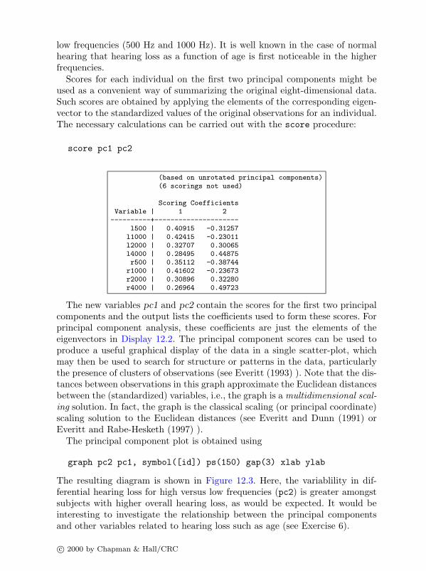
low frequencies (500 Hz and 1000 Hz). It is well known in the case of normalhearing that hearing loss as a function of age is first noticeable in the higherfrequencies.

Scores for each individual on the first two principal components might beused as a convenient way of summarizing the original eight-dimensional data.Such scores are obtained by applying the elements of the corresponding eigen-vector to the standardized values of the original observations for an individual.The necessary calculations can be carried out with the score procedure:

score pc1 pc2

(based on unrotated principal components)(6 scorings not used)

Scoring CoefficientsVariable | 1 2

----------+---------------------l500 | 0.40915 -0.31257

l1000 | 0.42415 -0.23011l2000 | 0.32707 0.30065l4000 | 0.28495 0.44875r500 | 0.35112 -0.38744

r1000 | 0.41602 -0.23673r2000 | 0.30896 0.32280r4000 | 0.26964 0.49723

The new variables pc1 and pc2 contain the scores for the first two principalcomponents and the output lists the coefficients used to form these scores. Forprincipal component analysis, these coefficients are just the elements of theeigenvectors in Display 12.2. The principal component scores can be used toproduce a useful graphical display of the data in a single scatter-plot, whichmay then be used to search for structure or patterns in the data, particularlythe presence of clusters of observations (see Everitt (1993) ). Note that the dis-tances between observations in this graph approximate the Euclidean distancesbetween the (standardized) variables, i.e., the graph is a multidimensional scal-ing solution. In fact, the graph is the classical scaling (or principal coordinate)scaling solution to the Euclidean distances (see Everitt and Dunn (1991) orEveritt and Rabe-Hesketh (1997) ).

The principal component plot is obtained using

graph pc2 pc1, symbol([id]) ps(150) gap(3) xlab ylab

The resulting diagram is shown in Figure 12.3. Here, the variablility in dif-ferential hearing loss for high versus low frequencies (pc2) is greater amongstsubjects with higher overall hearing loss, as would be expected. It would beinteresting to investigate the relationship between the principal componentsand other variables related to hearing loss such as age (see Exercise 6).


Figure 12.3 Principal component plot.

12.4 Exercises

1. Rerun the principal components analysis described in this chapter using thecovariance matrix of the observations. Compare the results with those basedon the correlation matrix.

2. Interpret components 3 through 8 in the principal components analysisbased on the correlation matrix.

3. Create a scatterplot matrix of the first five principal components scores.4. Investigate other methods of factor analysis available in factor applied to

the hearing data.5. Apply principal component analysis to the air pollution data analyzed in

Chapter 3, exluding the variable so2, and plot the first two principal compo-nents (i.e., the 2-d classical scaling solution for Euclidean distances betweenstandardized variables)

6. Regress so2 on the first two principal components and add a line correspond-ing to this regression (the direction of steapest increase in so2 predicted bythe regression plane) into the multidimenional scaling solution.


CHAPTER 13

Maximum Likelihood Estimation: Ageof Onset of Schizophrenia


In Table 13.1 the ages of onset of schizophrenia in 99 women (determined asage on first admission) are given. These data will be used in order to investi-gate whether there is any evidence for the subtype model of schizophrenia (seeLewine, 1981). According to this model, there are two types of schizophrenia.One is characterised by early onset, typical symptoms and poor premorbidcompetence and the other by late onset, atypical symptoms and good premor-bid competence. We will investigate this question by fitting a mixture of twonormal distributions to the ages.

13.2 Finite mixture distributions

The most common type of finite mixture distribution encountered in practiceis a mixture of univariate Gaussian distributions of the form

f(yi;p,µ,σ) = p1g(yi;µ1, σ1) + p2g(yi; µ2, σ2) + · · · + pkg(yi;µk, σk) (13.1)

where g(y;µ, σ) is the Gaussian density with mean µ and standard deviationσ,

g(y;µ, σ) =1

σ√

2πexp

{−1

2

(y − µ

σ

)2}

(13.2)

and p1, · · · , pk, are the mixing probabilities.The parameters p1, · · · , pk, µ1, · · · , µk and σ1, · · · , σk are usually estimated

by maximum likelihood. Standard errors may be obtained in the usual way fromthe observed information matrix (i.e., the inverse of the Hessian matrix, thematrix of second derivatives of the log-likelihood). Determining the numberof components in the mixture, k, is more problematic. This question is notconsidered here.

For a short introduction to finite mixture modeling, see Everitt (1996); amore comprehensive account is given in McLachlan and Basford (1988).


Table 13.1 Onset age of schizophrenia in 99 women. The data are in onset.dat

Age of onset

20 30 21 2330 25 13 1916 25 20 2527 43 6 2115 26 23 2123 23 34 1417 18 21 1635 32 48 5351 48 29 2544 23 36 5828 51 40 4321 48 17 2328 44 28 2131 22 56 6015 21 30 2628 23 21 2043 39 40 2650 17 17 2344 30 35 2041 18 39 2728 30 34 3330 29 46 3658 28 30 2837 31 29 3248 49 30


Stata has a set of commands, called ml, which can be used to maximize auser-specified log-likelihood using a modified Newton-Raphson algorithm. Thealgorithm is iterative. Starting with initial parameter estimates, the programevaluates the first and second derivatives of the log-likelihood in order to up-date the parameters in such a way that the log-likelihood is likely to increase.The updated parameters are then used to re-evalute the derivatives etc., un-til the program has converged to the maximum. The user needs to write aprogram which enables the ml program to evaluate the log-likelihood and itsderivatives.

There are four alternative methods available with ml, d0, d1, d2 and lf.The method d0 does not require the user’s program to evaluate any derivativesof the log-likelihood, d1 requires first derivatives only and d2 requires both firstand second derivatives. When d0 is chosen, first and second derivatives are


determined numerically; this makes this alternative slower and less accuratethan d1 or d2.

The simplest approach to use is lf which also does not require any derivativesto be programmed. Instead, the structure of most likelihood problems is usedto increase both the speed and accuracy of the numerical estimation of firstand second derivatives of the log-likelihood function. Whereas d0 to d2 can beused for any maximum likelihood problem, method lf may only be used if thelikelihood satisfies the following two criteria:

1. The observations in the dataset are independent, i.e., the log-likelihood isthe sum of the log-likelihood contributions of the observations.

2. The log-likelihood contributions have a linear form, i.e., they are (not nec-essarily linear) functions of linear predictors of the form ηi = x1iβi + · · · +xkiβk.

The first restriction is usually met, an exception being clustered data. Thesecond restriction is not as severe as it appears because there may be severallinear predictors, as we shall see later.

In this chapter we will give only a brief introduction to maximum likelihoodestimation using Stata, restricting our examples to the lf method. We recom-mend the book on Maximum Likelihood Estimation with Stata by Gould andSribney (1999) for a thorough treatment of the topic.

We will eventually fit a mixture of normals to the age of onset data, but willintroduce the ml procedure by a series of more simple steps. To begin with,we will fit a normal distribution with standard deviation fixed at 1 to a set ofsimulated data. A (pseudo)-random sample from the normal distribution withmean 5 and variance 1 may be obtained using the instructions

clearset obs 100set seed 12345678gen y = invnorm(uniform())+5

where the purpose of the set seed command is simply to ensure that thesame data will be generated each time. We use summarize to confirm that thesample has a mean close to 5 and a standard deviation close to 1.

summarize y


y | 100 5.002311 1.053095 2.112869 7.351898

First, define a program, mixing0, to evaluate the likelihood contributionswhen called from ml. The function must have two arguments; the first is thevariable name where ml will look for the computed log-likelihood contributions;


the second is the variable name containing the ‘current’ value of the linearpredictor during the iterative maximization procedure:

capture program drop mixing0program define mixing0

version 6args lj xb

tempname sscalar `s´ = 1tempvar f

quietly gen double `f´ = /**/ exp(-.5*(($ML_y1-`xb´)/`s´)^2)/(sqrt(2*_pi)*`s´)quietly replace `lj´ = ln(`f´)

end

After giving names lj and xb to the arguments passed to mixing0 by ml,mixing0 defines a temporary name stored in the local macro s and sets it equalto the standard deviation (1) in the next command. A temporary variable withits name stored in the local macro f is then defined to hold the normal densityfor each observation. The reason for defining s and f is to make subsequentcommands easier to read. Using temporary names avoids any confusion withvariables that may exist in the dataset and causes the scalar and variable todisappear when the program has finished running.

The normal density in equation (13.2) is a function of the difference betweenthe dependent variable, whose name is stored in the global macro ML y1 by mland the linear predictor or the mean `xb´. The final command replace `lj´=ln(`f´) places the log-likelihood functions into the variable `lj´as required bythe calling program.

Note that all variables defined within a program to be used with ml should beof storage type double to enable ml to estimate accurate numerical derivatives.Scalars should be used instead of local macros to hold constants as scalars havehigher precision.

The command

ml model lf mixing0 (xb: y=)

specifies the method as lf and the program to evaluate the log-likelihoodcontributions as mixing0.

The dependent and explanatory variable are specified by the “equation” inbrackets. The name before the colon, xb, is the name of the equation, thevariable name after the colon, y, is the dependent variable, and the variablenames after the ‘=’ give the explanatory variables for the linear predictor. Noexplanatory variables are given, so a constant only model will be fitted.


As a result of this model definition, ML y1 will be equal to y and in mixing0`xb´ will be equal to the intercept parameter (the mean) that is going to beestimated by ml.

Now maximize the likelihood using

ml maximize

giving the results shown in Display 13.1. The program converged in three itera-

initial: log likelihood = -1397.9454alternative: log likelihood = -1160.3298rescale: log likelihood = -197.02113Iteration 0: log likelihood = -197.02113Iteration 1: log likelihood = -146.79076Iteration 2: log likelihood = -146.78981Iteration 3: log likelihood = -146.78981

Number of obs = 100Wald chi2(0) = .

Log likelihood = -146.78981 Prob > chi2 = .


---------+--------------------------------------------------------------------_cons | 5.002311 .1 50.023 0.000 4.806314 5.198307

------------------------------------------------------------------------------

Display 13.1

tions and the maximum likelihood estimate of the mean is equal to the samplemean of 5.002311. If we are interested in observing the change in the estimateof the mean in each iteration, we can use the trace option in the ml maximizecommand. The Wald chi2(0) output is empty because we have not specifieda likelihood with which to compare the current model. We can suppress thisuninformative output using ml maximize with the noheader option.

We now need to extend the program step by step until it can be used toestimate a mixture of two Gaussians. The first step is to allow the standarddeviation to be estimated. Since this parameter does not contribute linearlyto the linear predictor used to estimate the mean, we need to define anotherlinear predictor by specifying another equation with no dependent variable inthe ml model command as follows:

ml model lf mixing1 (xb: y=) (lsd:)

The new equation has the name lsd, has no dependent variable and the linearpredictor is simply a constant. A short-form of the above command is

ml model lf mixing1 (xb: y=) /lsd

We intend to use lsd as the log-standard deviation. Estimating the log of the


standard deviation will ensure that the standard deviation itself is positive. Wenow need to modify the function mixing0 so that it has an additional argumentfor the log standard deviation.


version 6.0args lj xb ls

tempvar f s

quietly gen double `s´ = exp(`ls´)quietly gen double `f´ = /**/ exp(-.5*(($ML_y1-`xb´)/`s´)^2)/(sqrt(2*_pi)*`s´)quietly replace `lj´ = ln(`f´)

end

In mixing1, s is now the name of a variable instead of a scalar because,in principal, the linear predictor `ls´, defined in the ml model command,may contain covariates (see exercises) and hence differ between observations.Making these changes and using

ml maximize

gives the output shown in Display 13.2.

initial: log likelihood = -1397.9454alternative: log likelihood = -534.94948rescale: log likelihood = -301.15405rescale eq: log likelihood = -180.56802Iteration 0: log likelihood = -180.56802Iteration 1: log likelihood = -146.65085Iteration 2: log likelihood = -146.56478Iteration 3: log likelihood = -146.56469Iteration 4: log likelihood = -146.56469------------------------------------------------------------------------------

y | Coef. Std. Err. z P>|z| [95% Conf. Interval]---------+--------------------------------------------------------------------xb |

_cons | 5.002311 .1047816 47.740 0.000 4.796942 5.207679---------+--------------------------------------------------------------------lsd |

_cons | .0467083 .0707107 0.661 0.509 -.091882 .1852987------------------------------------------------------------------------------

Display 13.2

The standard deviation estimate is obtained by taking the exponential ofthe estimated coefficient of cons in equation lsd. Instead of typing displayexp(0.0467083), we can use following the syntax for accessing coefficients andtheir standard errors:


display [lsd] b[ cons]

.04670833

display [lsd] se[ cons]

.07071068

We can also omit “ b” from the first expression and compute the requiredstandard deviation using

display exp([lsd][ cons])

1.0478163

This is smaller than the sample standard deviation from summarize becausethe maximum likelihood estimate of the standard deviation is given by

σ =

√√√√ 1n

n∑i=1

(yi − y)2 (13.3)

where n is the sample size, whereas the factor 1n−1 is used in summarize. Since

n is 100 in this case, the maximum likelihood estimate must be blown up by afactor of

√100/99 to obtain the sample standard deviation:

display exp([lsd][ cons])*sqrt(100/99)

1.053095

The program can now be extended to estimate a mixture of two Gaussians.In order to be able to test the program on data from a known distribution,we will generate a sample from a mixture of two Gaussians with variances of1 and means of 0 and 5 and with mixing probabilities p1 = p2 = 0.5. This canbe done in two stages; first randomly allocate observations to groups (variablez) with probabilities p1 and p2 and then sample from the different componentdensities according to group membership.

clearset obs 300set seed 12345678gen z = cond(uniform()<0.5,1,2)gen y = invnorm(uniform())replace y = y + 5 if z==2

We now need five equations, one for each parameter to be estimated: µ1,µ2, σ1, σ2 and p1 (since p2 = 1 − p1). As before, we can ensure that the


estimated standard deviations are positive by taking the exponential insidethe program. The mixing proportion p1 must lie in the range 0 ≤ p1 ≤ 1. Oneway of ensuring this is to interpret the linear predictor as representing the logodds (see Chapter 6) so that p1 is obtained from the linear predictor of the logodds, lo1 using the transformation 1/(1+exp(-lo1)). The program mixing1now becomes


version 6.0args lj xb xb2 lo1 ls1 ls2

tempvar f1 f2 p s1 s2

quietly gen double `s1´ = exp(`ls1´)quietly gen double `s2´ = exp(`ls2´)quietly gen double `p´ = 1/(1+exp(-`lo1´))

quietly gen double `f1´ = /**/ exp(-.5*(($ML_y1-`xb´)/`s1´)^2)/(sqrt(2*_pi)*`s1´)quietly gen double `f2´ = /**/ exp(-.5*(($ML_y1-`xb2´)/`s2´)^2)/(sqrt(2*_pi)*`s2´)quietly replace `lj´ = ln(`p´*`f1´ + (1-`p´)*`f2´)

end

Stata simply uses the value 0 as the initial value for all parameters. Whenfitting a mixture distribution, it is not advisable to start with the same initialvalue for both means. Therefore, the initial values should be set. This can bedone using the ml init command between the ml model and ml maximizecommands as follows:

ml model lf mixing2 (xb1: y=) /xb2 /lo1 /lsd1 /lsd2ml init 1 6 0 0.2 -0.2, copyml maximize, noheader

The first two values will be the initial values for the means, the third theinitial log odds and the third and fourth the initial values of the logs of thestandard deviations. The results are shown in Display 13.3

The standard deviations are therefore estimated as

display exp([lsd1][ cons])

.97290582

and


initial: log likelihood = -746.68918rescale: log likelihood = -746.68918rescale eq: log likelihood = -676.61764Iteration 0: log likelihood = -676.61764 (not concave)Iteration 1: log likelihood = -630.71045Iteration 2: log likelihood = -625.88875Iteration 3: log likelihood = -622.23405Iteration 4: log likelihood = -622.21162Iteration 5: log likelihood = -622.21162------------------------------------------------------------------------------

y | Coef. Std. Err. z P>|z| [95% Conf. Interval]---------+--------------------------------------------------------------------xb1 |

_cons | -.0457452 .0806427 -0.567 0.571 -.203802 .1123117---------+--------------------------------------------------------------------xb2 |

_cons | 4.983717 .0863492 57.716 0.000 4.814476 5.152958---------+--------------------------------------------------------------------lo1 |

_cons | .1122415 .1172032 0.958 0.338 -.1174725 .3419555---------+--------------------------------------------------------------------lsd1 |

_cons | -.027468 .0627809 -0.438 0.662 -.1505164 .0955804---------+--------------------------------------------------------------------lsd2 |

_cons | -.0173444 .0663055 -0.262 0.794 -.1473008 .1126121------------------------------------------------------------------------------

Display 13.3

display exp([lsd2][ cons])

.9828052

and the probability of membership in group 1 is

display 1/(1 + exp(-[lo1][ cons]))

.52803094

Alternative estimates of mixing proportion and means and standard deviations,knowing group membership in the sample, are obtained using

table z, contents(freq mean y sd y)

----------+-----------------------------------z | Freq. mean(y) sd(y)

----------+-----------------------------------1 | 160 -.0206726 1.0032542 | 140 5.012208 .954237

----------+-----------------------------------

The estimated parameters agree quite closely with the true parameters and


with those estimated by knowing the group membership. The true proportionwas 0.5 and the realized proportion is 160/300 = 0.53, also very close to themaximum likelihood estimate.

The standard errors of the estimated means are given in the regression ta-ble in Display 13.3 (0.081 and 0.086). We can estimate the standard errorsof the standard deviations and of the probability from the standard errorsof the log standard deviations and log odds using the delta-method (see forexample Dunn, 1989). According to the delta-method, if y = f(x), then ap-proximately, se(y) = |f ′(x)|se(x) where f ′(x) is the first derivative of f(x) withrespect to x evaluated at the estimated value of x. For the standard deviation,sd = exp(lsd), so that, by the delta method,

se(sd) = sd ∗ se(lsd). (13.4)

For the probability, p = 1/(1 + exp(−lo)), so that

se(p) = p(1 − p) ∗ se(lo). (13.5)

The approximate standard errors for the standard deviations are therefore

scalar x = exp([lsd1][_cons])display [lsd1]_se[_cons]*scalar(x)

.06107994

scalar x = exp([lsd2][_cons])display [lsd2]_se[_cons]*scalar(x)

.06516543

and for the probability

scalar x = 1/(1 + exp(-[lo1][_cons]))display [lo1]_se[_cons]*scalar(x*(1-x))

.0292087

In the above commands, the function scalar() was used to make sure thatx is interpreted as the scalar we have defined and not as a variable we mayhappen to have in the dataset. This was not necessary in the program mixing2because there we used a temporary name; temporary names look somethinglike 0009J4 and are defined deliberately to be different to any variable namein the dataset.

We can now apply the same program to the age of onset data. The data canbe read in using

infile y using onset.dat, cleargen ly=ln(y)label variable y "age of onset of schizophrenia"


A useful graphical display of the data is a histogram found from

graph y, hist bin(10) xlab ylab gap(3)

which is shown in Figure 13.1.

Figure 13.1 Histogram of age of onset of schizophrenia in women.

It seems reasonable to use initial values of 20 and 45 for the two means. Inaddition, we will use a mixing proportion of 0.5 and log standard deviationsof 2 as initial values.

ml model lf mixing2 (y: y=) /xb2 /lo1 /lsd1 /lsd2ml init 20 45 0 2 2, copyml maximize, noheader

The output is given in Display 13.4. The means are estimated as 24.8 and46.4 the standard deviations are estimated as 6.5 and 7.1 for groups 1 and2, respectively, and the mixing proportions are estimated 0.74 and 0.26. Theapproximate standard errors may be obtained as before; see exercises. Thehistogram strongly suggests that there are two subpopulations. In order to testthis more formally, we could also fit a single normal distribution and comparethe likelihoods. Wolfe (1971) suggests, on the basis of a limited simulationstudy, that the difference in minus twice the log-likelihood for a model with c


initial: log likelihood = -391.61146rescale: log likelihood = -391.61146rescale eq: log likelihood = -391.61146Iteration 0: log likelihood = -391.61146 (not concave)Iteration 1: log likelihood = -374.66666 (not concave)Iteration 2: log likelihood = -374.36519Iteration 3: log likelihood = -373.93993Iteration 4: log likelihood = -373.67089Iteration 5: log likelihood = -373.66896Iteration 6: log likelihood = -373.66896------------------------------------------------------------------------------

y | Coef. Std. Err. z P>|z| [95% Conf. Interval]---------+--------------------------------------------------------------------xb1 |

_cons | 24.79772 1.133545 21.876 0.000 22.57601 27.01942---------+--------------------------------------------------------------------xb2 |

_cons | 46.44685 2.740866 16.946 0.000 41.07485 51.81885---------+--------------------------------------------------------------------lo1 |

_cons | 1.034415 .3697502 2.798 0.005 .3097178 1.759112---------+--------------------------------------------------------------------lsd1 |

_cons | 1.877698 .1261092 14.889 0.000 1.630529 2.124868---------+--------------------------------------------------------------------lsd2 |

_cons | 1.955009 .25692 7.609 0.000 1.451455 2.458563------------------------------------------------------------------------------

Display 13.4

components compared with a model with c+1 components has approximatelya χ2 distribution with 2ν−2 degrees of freedom where ν is the number of extraparameters in the c + 1 component mixture. The log-likelihood of the currentmodel may be accessed using e(ll). We store this in a local macro

local ll = e(ll)

and fit the single normal model using the program mixing1 as follows:ml model lf mixing1 (xb: y=) /lsdml init 30 1.9, copyml maximize, noheader

with the result shown in Display 13.5We can now compare the log-likelihoods using the method proposed by

Wolfe:

local chi2 = 2*(`ll´-e(ll))display chiprob(4,`chi2´)

.00063994

This test confirms that there appear to be two subpopulations.


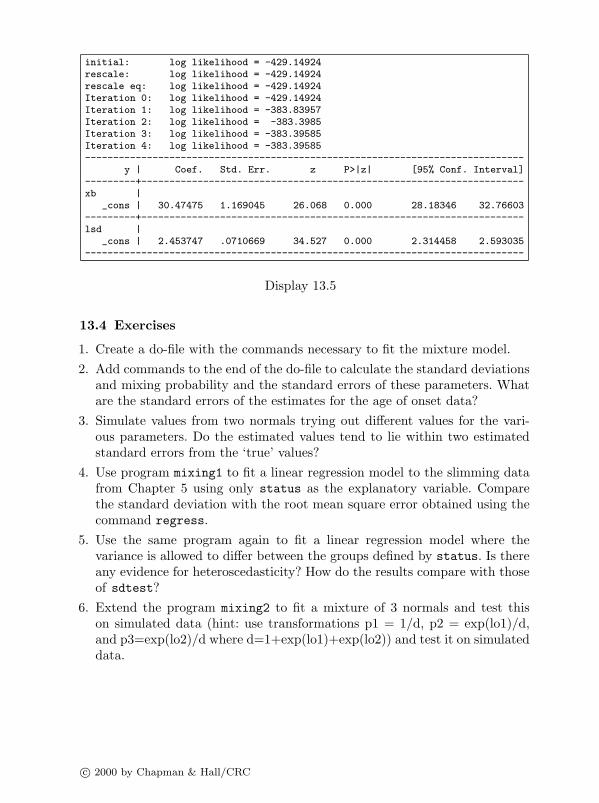
initial: log likelihood = -429.14924rescale: log likelihood = -429.14924rescale eq: log likelihood = -429.14924Iteration 0: log likelihood = -429.14924Iteration 1: log likelihood = -383.83957Iteration 2: log likelihood = -383.3985Iteration 3: log likelihood = -383.39585Iteration 4: log likelihood = -383.39585------------------------------------------------------------------------------

y | Coef. Std. Err. z P>|z| [95% Conf. Interval]---------+--------------------------------------------------------------------xb |

_cons | 30.47475 1.169045 26.068 0.000 28.18346 32.76603---------+--------------------------------------------------------------------lsd |

_cons | 2.453747 .0710669 34.527 0.000 2.314458 2.593035------------------------------------------------------------------------------

Display 13.5

13.4 Exercises

1. Create a do-file with the commands necessary to fit the mixture model.2. Add commands to the end of the do-file to calculate the standard deviations

and mixing probability and the standard errors of these parameters. Whatare the standard errors of the estimates for the age of onset data?

3. Simulate values from two normals trying out different values for the vari-ous parameters. Do the estimated values tend to lie within two estimatedstandard errors from the ‘true’ values?

4. Use program mixing1 to fit a linear regression model to the slimming datafrom Chapter 5 using only status as the explanatory variable. Comparethe standard deviation with the root mean square error obtained using thecommand regress.

5. Use the same program again to fit a linear regression model where thevariance is allowed to differ between the groups defined by status. Is thereany evidence for heteroscedasticity? How do the results compare with thoseof sdtest?

6. Extend the program mixing2 to fit a mixture of 3 normals and test thison simulated data (hint: use transformations p1 = 1/d, p2 = exp(lo1)/d,and p3=exp(lo2)/d where d=1+exp(lo1)+exp(lo2)) and test it on simulateddata.


Appendix: Answers to SelectedExercises

Chapter 1

Assuming that the data are stored in the directory c:\user,2. cd c:\user

insheet using test.dat, clear

4. label define s 1 male 2 femalelabel values sex s

5. gen id=_n

6. rename v1 time1rename v2 time2rename v3 time3

or

for var v1-v3 \ num 1/3: rename X timeY

7. reshape long time, i(id) j(occ)

8. egen d=mean(time), by(id)replace d=(time-d)^2

9. drop if occ==3&id==2

Chapter 2

1. table depress, contents(mean weight)

2. for var iq age weight: table life, contents(mean X sd X)

3. search mannhelp signrank

4. ranksum weight, by(life)

5. gen iq1=iq if life==2gen iq2=iq if life==1label variable iq1 "no"label variable iq2 "yes"graph iq1 iq2 age, s(dp) xlabel ylabel jitter(2) l1("IQ")


6. Save the commands in the “Review” window and edit the file using theDo-file Editor or any texteditor, e.g., Notepad. Add the commands given inthe do-file template in Section 1.9 and save the file with the extension .do.Run the file by typing the command do filename.

Chapter 4

1. infile bp11 bp12 bp13 bp01 bp02 bp03 using bp.raw

2. sort druggraph bp, box by(drug)sort dietgraph bp, box by(diet)sort biofeedgraph bp, box by(biofeed)

4. sort idsave bpinfile id age using age.dat, clearsort idmerge id using bpanova bp drug diet biofeed age, continuous(age)

Chapter 5

1. anova resp cond*status status cond, sequential

2. gen dcond=cond-1gen dstat=status-1gen dinter=dcond*dstatregress resp dcond dstat dinter

3. xi: regress resp i.cond*i.status

4. char cond[omit] 2char status[omit] 2xi: regress resp i.cond*i.status

Chapter 6

1. ologit outc therapy sex [fweight=fr], table

2.(a) ologit depress life

(b) replace life=life-1logistic life depress

3. Even if we use very lenient inclusion and exclusion criteria,


sw logistic life depress anxiety iq sex sleep, /**/ pr(0.2) pe(0.1) forward

only depress is selected. If we exclude depress from the list of candidatevariables, anxiety and sleep are selected.

4. bprobit pres tot ckpredict predpgraph predp prop ck, c(s.)

Chapter 7

1. xi: glm resp i.cond i.status, fam(gauss) link(id)local dev1=e(deviance)xi: glm resp i.cond, fam(gauss) link(id)local dev2=e(deviance)local ddev=`dev2´-`dev1´/* F-test equivalent to anova cond status, sequential */local f=(`ddev´/1)/(`dev1´/31)disp `f´disp fprob(1,31,`f´)/* difference in deviance */disp `ddev´disp chiprob(1, `ddev´)

2. reg resp status, robustttest resp, by(status) unequal

3. gen cleth=class*ethnicglm days class ethnic cleth, fam(poiss) link(log)

4. glm days class ethnic if stres<4, fam(poiss) link(log)

or, assuming the data has not been sorted,

glm days class ethnic if _n~=72, fam(poiss) link(log)

5. gen abs=cond(days>=14,1,0)glm abs class ethnic, fam(binomial) link(logit)glm abs class ethnic, fam(binomial) link(probit)

6. logit abs class ethnic, robustprobit abs class ethnic, robustbs "logit abs class ethnic" "_b[class] _b[ethnic]", reps(500)bs "probit abs class ethnic" "_b[class] _b[ethnic]", reps(500)

Chapter 8

1. graph dep1-dep6, box by(group)


2. We can obtain the mean over visits for subjects with complete data usingthe simple command (data in ‘wide’ form)

gen av2 = (dep1+dep2+dep3+dep4+dep5+dep6)/6

The t-tests are obtained using

ttest av2, by(group)ttest av2, by(group) unequal

3. egen avg = rmean(dep1-dep6)egen sd = rsd(dep1-dep6)gen stdav= avg/sdttest stdav, by(group)

4.(a) gen diff = avg-prettest diff, by(group)

(b) anova avg group pre, continuous(pre)

Chapter 9

2.(a) infile subj group pre dep1 dep2 dep3 dep4 dep5 dep6 /**/ using depress.dat

mvdecode _all, mv(-9)reshape long dep, i(subj) j(visit)reg dep group pre visit, robust cluster(subj)

(b) bs "reg dep group pre visit" "_b[group] _b[pre] _b[visit]", /**/ cluster(subj) reps(500)

5. infile subj y1 y2 y3 y4 treat baseline age using chemo.datreshape long y, i(subj) j(week)expand 2 if week==1sort subj weekqui by subj: replace week=0 if _n==1replace y=baseline/4 if week==0gen post=week!=0xi: xtgee y i.treat*i.post age, i(subj) t(week) corr(exc) /*

*/ family(pois) scale(x2) eform

Chapter 10

1. infile v1-v2 using estrogen.dat, cleargen str8 _varname="ncases1" in 1replace _varname="ncases0" in 2xpose,cleargen conestr=2-_nreshape long ncases, i(conestr) j(casestr)


expand ncasessort casestr conestrgen caseid=_nexpand 2sort caseidquietly by caseid: gen control=_n-1 /*control=1,case=0 */gen estr=0replace estr=1 if control==0&casestr==1replace estr=1 if control==1&conestr>0gen cancer=control==0clogit cancer estr, group(caseid) or

2. table exposed, contents(sum num sum py)iri 17 28 2768.9 1857.5

3. xi: poisson num i.age*exposed, e(py) irrtestparm IaX*

The interaction is not statistically significant at the 5% level.4. infile subj y1 y2 y3 y4 treat baseline age using chemo.dat

reshape long y, i(subj) j(week)expand 2 if week==1sort subj weekqui by subj: replace week=0 if _n==1replace y=baseline if week==0gen post=week!=1gen ltime=log(cond(week==0,8,2))xi: xtgee y i.treat*i.post age , i(subj) t(week) corr(exc) /*

*/ family(pois) scale(x2) offset(ltime)

Chapter 11

1. We consider anyone still at risk after 450 days as being censored at 450 daysand therefore need to make the appropriate changes to status and timebefore running Cox regression.

replace status=0 if time>450replace time=450 if time>450stset time, failure(status)stcox dose prison clinic

2. The model is fitted using

gen dose_cat=0 if dose~=.replace dose_cat=1 if dose>=60replace dose_cat=2 if dose>=80xi: stcox i.dose_cat i.prison i.clinic, bases(s)


The survival curves for no prison record, clinic 1 are obtained using

gen s0 = s if dose_cat==0gen s1 = s^(exp(_b[Idose__1]))gen s2 = s^(exp(_b[Idose__2]))graph s0 s1 s2 time, sort c(JJJ) s(...) xlab ylab gap(3)

Note that the baseline survival curve is the survival curve for someone whosecovariates are all zero. If we had used clinic instead of i.clinic above,this would have been meaningless; we would have had to exponentiate s0,s1 and s2 by b[clinic] to calculate the survival curves for clinic 1.

3. Treating dose as continuous:

gen clindose=clinic*dosestcox dose prison clinic clindose

Treating dose as categorical:

xi: stcox i.dose_cat*i.clinic i.prisontestparm IdX*

5. gen tpris=prison*(t-504)/365.25stcox dose prison tpris, strata(clinic)lrtest, saving(0)stcox dose prison, strata(clinic)lrtest

Chapter 12

1. factor l500-r4000, pc cov

3. capture drop pc*factor l500-r4000, pcscore pc1-pc5graph pc1-pc5, matrix

5. infile str10 town so2 temp manuf pop wind precip days using usair.datfactor temp manuf pop wind precip days,pcscore pc1 pc2graph pc2 pc1, symbol([town]) ps(150) gap(3) xlab ylab

6. regress so2 pc1 pc2gen line=pc1*_b[pc2]/_b[pc1]graph pc2 line pc1, s([town]i) c(.l) ps(150) gap(3) xlab ylab

Chapter 13

2. scalar x = exp([lsd1][_cons])disp "st. dev. 1 = " scalar(x) ", standard error = " /*


*/ [lsd1]_se[_cons]*scalar(x)

scalar x = exp([lsd2][_cons])disp "st. dev. 2 = " scalar(x) ", standard error = " /*

*/ [lsd2]_se[_cons]*scalar(x)

scalar x = 1/(1 + exp(-[lo1][_cons]))disp "probability = " scalar(x) ", standard error = "/*

*/ [lo1]_se[_cons]*scalar(x*(1-x))

giving the results

st. dev. 1 = 6.5384366, standard error = .82455744st. dev. 2 = 7.0639877, standard error = 1.8148844probability = .7377708, standard error = .07153385

4. The only thing that is different from fitting a normal distribution withconstant mean is that the mean is now a linear function of status so thatthe ml model command changes as shown below

infile cond status resp using slim.dat, clearml model lf mixing1 (xb: resp = status) /lsdml maximize, noheader

In linear regression, the mean square error is equal to the sum of squaresdivided by the degrees of freedom, n-2. The maximum likelihood estimateis equal to the sum of squares divided by n. We can therefore get the rootmean square error for linear regression using

disp exp([lsd][_cons])*sqrt(_N/(_N-2))

Note that the standard error of the regression coefficients need to be cor-rected by the same factor, i.e.,

disp [xb]_se[status]*sqrt(_N/(_N-2))

Compare this with the result of

regress resp status

5. Repeat the procedure above but replace the ml model command by

ml model lf mixing1 (resp = status) (lsd: status)

The effect of status on the standard deviation is significant (p=0.003)which is not too different from the result of

sdtest resp, by(status)

6. capture program drop mixing3program define mixing3


version 6.0args lj xb xb2 xb3 lo1 lo2 ls1 ls2 ls3

tempvar f1 f2 f3 p1 p2 p3 s1 s2 s3 d

quietly gen double `s1´ = exp(`ls1´)quietly gen double `s2´ = exp(`ls2´)quietly gen double `s3´ = exp(`ls3´)quietly gen double `d´ = 1 + exp(`lo1´) + exp(`lo2´)quietly gen double `p1´ = 1/`d´quietly gen double `p2´ = exp(`lo1´)/`d´quietly gen double `p3´ = exp(`lo2´)/`d´

quietly gen double `f1´ = /**/ exp(-.5*(($ML_y1-`xb´)/`s1´)^2)/(sqrt(2*_pi)*`s1´)quietly gen double `f2´ = /**/ exp(-.5*(($ML_y1-`xb2´)/`s2´)^2)/(sqrt(2*_pi)*`s2´)quietly gen double `f3´ = /**/ exp(-.5*(($ML_y1-`xb3´)/`s3´)^2)/(sqrt(2*_pi)*`s3´)quietly replace `lj´ = ln(`p1´*`f1´ + `p2´*`f2´ + `p3´*`f3´)

end

clearset obs 300set seed 12345678gen z = uniform()gen y = invnorm(uniform())replace y = y + 5 if z<1/3replace y = y + 10 if z<2/3&z>=1/3ml model lf mixing3 (xb1: y=) /xb2 /xb3 /lo1 /lo2 /lsd1 /lsd2 /lsd3ml init 0 5 10 0 0 0 0 0, copyml maximize, noheader trace


References

Aitkin, M. 1978. The analysis of unbalanced cross-classifications (with discussion).Journal of the Royal Statistical Society, A, 41, 195–223.

Binder, D. A. 1983. On the variances of asymptotically normal estimators fromcomplex surveys. International Statistical Review, 51, 279–292.

Boniface, D. R. 1995. Experimental Design and Statistical Methods. London: Chap-man & Hall.

Caplehorn, J., & Bell, J. 1991. Methadone dosage and the retention of patients inmaintenance treatment. The Medical Journal of Australia, 154, 195–199.

Chatterjee, S., & Price, B. 1991. Regression Analysis by Example (2nd Edition). NewYork: Wiley.

Clayton, D., & Hills, M. 1993. Statistical Models in Epidemiology. Oxford: OxfordUniversity Press.

Collett, D. 1991. Modelling Binary Data. London: Chapman & Hall.Collett, D. 1994. Modelling Survival Data in Medical Research. London: Chapman

& Hall.Cook, R. D. 1977. Detection of influential observations in linear regression. Techno-

metrics, 19, 15–18.Cook, R. D. 1979. Influential observations in linear regression. Journal of the Amer-

ican Statistical Association, 74, 164–174.Cook, R. D., & Weisberg, S. 1982. Residuals and Influence in Regression. London:

Chapman & Hall.Diggle, P. J., Liang, K-Y, & Zeger, S. L. 1994. Analysis of Longitudinal Data. Oxford:

Oxford University Press.Dunn, G. 1989. Design and Analysis of Reliability Studies. Oxford: Oxford University

Press.Efron, B., & Tibshirani, R. 1993. An Introduction to the Bootstrap. London: Chapman

& Hall.Everitt, B. S. 1993. Cluster Analysis. London: Edward Arnold.Everitt, B. S. 1994. Statistical Methods for Medical Investigations. London: Edward

Arnold.Everitt, B. S. 1995. The analysis of repeated measures: A practical review with

examples. The Statistician, 44, 113–135.Everitt, B. S. 1996. An introduction to finite mixture distributions. Statistical Meth-

ods in Medical Research, 5, 107–127.Everitt, B. S., & Der, G. 1996. A Handbook fo Statistical Analyses using SAS. London:

Chapman & Hall.Everitt, B. S., & Dunn, G. 1991. Applied Multivariate Analysis. London: Edward

Arnold.


Everitt, B. S., & Rabe-Hesketh, S. 1997. The Analysis of Proximity Data. London:Edward Arnold.

Goldstein, H. 1995. Multilevel Statistical Models. London: Edward Arnold.Gould, W. 1999. Estimating a cox model with continuously time-varying parameter.

Stata FAQ.Gould, W., & Sribney, W. 1999. Maximum Likelihood Estimation with Stata. College

Station, TX: Stata Press.Gregoire, A. J. P., Kumar, R., Everitt, B. S., Henderson, A. F., & Studd, J. W. W.

1996. Transdermal oestrogen for the treatment of severe post-natal depression.The Lancet, 347, 930–934.

Hamilton, L. C. 1998. Statistics with Stata 5. Belmont, CA: Duxbury Press.Hand, D. J., & Crowder, M. 1996. Practical Longitudinal Data Analysis. London:

Chapman & Hall.Hand, D. J., Daly, F., Lunn, A. D., McConway, K. J., & Ostrowski, E. 1994. A

Handbook of Small Data Sets. London: Chapman & Hall.Holtbrugge, W., & Schumacher, M. 1991. A comparison of regression models for the

analysis of ordered categorical data. Applied Statistics, 40, 249–259.Hotelling, H. 1933. Analysis of complex statistical variables into principal compo-

nents. Journal of Education Psychology, 24, 417–441.Jackson, J. E. 1991. A User’s Guide to Principal Components. New York: Wiley.Jennrich, R. I., & Schluchter, M. D. 1986. Unbalanced repeated measures models

with unstructured covariance matrices. Biometrics, 42, 805–820.Lachenbruch, P., & Mickey, R. M. 1986. Estimation of error rates in discriminant

analysis. Technometrics, 10, 1–11.Lewine, R. R. J. 1981. Sex differences in schizophrenia: timing or subtypes? Psycho-

logical Bulletin, 90, 432–444.Liang, K-Y., & Zeger, S. L. 1986. Longitudinal data analysis using generalised linear

models. Biometrika, 73, 13–22.Mallows, C. L. 1986. Some comments on Cp. Technometrics, 15, 661–675.Manly, B. F. J. 1997. Randomisation, Bootstrap and Monte Carlo Methods in Biology.

London: Chapman & Hall.Mathews, J. N. S., Altman, D. G., Campbell, M. J., & Royston, P. 1990. Analysis of

seriel measurements in medical research. British Medical Journal, 300, 230–235.Maxwell, S. E., & Delaney, H. D. 1990. Designing Experiments and Analysing Data.

California: Wadsworth.McCullagh, P., & Nelder, J. A. 1989. Generalized Linear Models. London: Chapman

& Hall.McKay, R. J., & Campbell, N. A. 1982a. Variable selection techniques in discriminant

analysis. I Description. British Journal of Mathematical and Statistical Psychology,35, 1–29.

McKay, R. J., & Campbell, N. A. 1982b. Variable selection techniques in discriminantanalysis. II Allocation. British Journal of Mathematical and Statistical Psychology,35, 30–41.

McLachlan, G. J., & Basford, K. E. 1988. Mixture Models; Inference and Applicationto Clustering. New York: Marcel Dekker, Inc.

Nelder, J. A. 1977. A reformulation of linear models. Journal of the Royal StatisticalSociety, A, 140, 48–63.


Pearson, K. 1901. On lines and planes of closest fit to points in space. PhilosophicalMagazine, 2, 559–572.

Rawlings, J. O. 1988. Applied Regression Analysis. California: Wadsworth Books.Rothman, K. J. 1986. Modern Epidemiology. Boston: Little, Brown & Company.Sackett, D. L., Haynes, R. B., Guyatt, G. H., & Tugwell, P. 1991. Clinical Epidemi-

ology. Massachusetts: Little Brown & Company.Sokal, R. R., & Rohlf, F. J. 1981. Biometry. San Francisco: W. H. Freeman.Sprent, P. 1993. Applied Nonparametric Statistical Methods. Chapman & Hall: P.

Sprent.Sribney, B. 1998. What are the advantages of using robust variance estimators over

standard maximum-likelihood estimators in logistic regression. Stata FAQ.Stata Getting Started 1999. Getting Started with Stata for Windows. College Station,

TX: State Press.Stata Graphics Manual. 1999. Stata Graphics Manual. College Station, TX: State

Press.Stata Manuals 1-4. 1999. Stata Reference Manuals. College Station, TX: State Press.Stata User’s Guide. 1999. Stata User’s Guide. College Station, TX: State Press.Thall, P. F., & Vail, S. C. 1990. Some covariance models for longitudinal count data

with overdispersion. Biometrics, 46, 657–671.Wedderburn, R. W. M. 1974. Quasilikelihoodfunctions, generalised linear models and

the Gauss-Newton method. Biometrika, 61, 439–47.Winer, B. J. 1971. Statistical Principles in Experimental Design. New York: McGraw-

Hill.Wolfe, J. H. 1971. A Monte Carlo study of the sampling distribution of the likelihood

ratio for mixtures of multinormal distributions. Technical Bulletin, vol. STB72-2.San Diego: Naval Personnel and Training Research Laboratory.


Statistical Analysisi Usin STATA

Documents

Transcript of Statistical Analysisi Usin STATA