STAR and ANN models: Forecasting performance on the Spanish “Ibex-35” stock index

Jorge V. Pérez-Rodríguez

Department of Quantitative Methods University of Las Palmas de Gran Canaria

Campus de Tafira, Tafira Baja. E-35017, Las Palmas. Spain

Phone:+34 928 458222 y Fax: +34 928-458225 / 1829 (Email: jorge@empresariales.ulpgc.es)

Salvador Torra

Department of Econometrics, Statistics and Spanish Economy University of Barcelona

(Email: storra@eco.ub.es )

and

Julian Andrada-Félix

Department of Quantitative Methods University of Las Palmas de Gran Canaria

(Email: julian@empresariales.ulpgc.es)

Corresponding author: Dr. Jorge V. Pérez-Rodríguez Department of Quantitative Methods University of Las Palmas de Gran Canaria Campus de Tafira, Tafira Baja. E-35017, Las Palmas. Spain

1

Abstract: This paper examines the out-of-sample forecast performance of smooth transition

autoregressive (STAR) models and artificial neural networks (ANNs) when applied to daily

returns on the Ibex-35 stock index, during the period from 30 December 1989 to 10

February 2000. The forecasts are evaluated with statistical criteria such as goodness of

forecast, including tests of forecast encompassing, directional accuracy and the equality of

mean squared prediction error; the relative forecast performance is assessed with economic

criteria in a simple trading strategy including the impact of transaction costs on trading

strategy profits. In terms of statistical criteria, the results show that different artificial neural

network specifications forecast better than the AR model and smooth transition non-linear

models. In terms of the economic criteria in the out-of-sample forecasts, we assess

profitability and combine a simple trading strategy known as the filter technique by using a

range filter percentage and trading costs. The results indicate a better fit for ANN models,

in terms of the Sharpe risk-adjusted ratio. These results show there is a good chance of

obtaining a more accurate fit and forecast of the daily stock index returns by using non-

linear models, but that these are inherently complex and present a difficult economic

interpretation.

Keywords : Non- linearities, statistical criteria, trading strategies.

JEL classifications: C22, C45, C52.

2

1. Introduction

Some researchers have questioned the hypothesis of Efficient Markets (HEM), i.e. that

the random walk model is a reasonable description of asset price movement and that linear

models successfully describe the evolution of such prices. For example, Hinich and

Paterson (1985), Cochrane (1988), Fama and French (1988), Lo and McKinlay (1988),

White (1988), Sheinkman and LeBaron (1989), Hsieh (1991), Granger (1992), Gençay

(1996), Campbell, Lo and McKinlay (1997), De Lima (1998), Fernández, García and

Sosvilla (1999) and García and Gençay (2000) have raised the question of whether the

behaviour of asset returns is completely random; whether linear modelling techniques are

appropriate to capture some of the complex models that chartists have observed in the

evolution of asset prices and the market negotiation process; whether it is possible to

identify and exploit the behaviour of asset returns over time; or whether the adjustments

made in the market in response to price deviations and their theoretical value might not be

proportional to the quantity by which prices deviate from their real value.

Theoretical and practical interest in non-linear time series models has increased rapidly

in recent years. Various factors might account for non-linearity. On the one hand, we could

admit the possibility that not all the agents simultaneously receive all the information; there

may be important differences in targets and in negotiation time; or those agents with more

complex algorithms might be able to make better use of the available information1.

However, there are several reasons why non- linear modelling is not easy. First, because

there exist a great number of options, i.e. bilinear models, ARCH and its extensions,

smooth transition autoregressive models (STAR), artificial neural networks (ANN),

wavelets and even chaotic dynamics. Second, because the flexibility inherent in its use can

create spurious fits [Granger and Teräsvirta (1993)]; and third, because when considering a

long period of time there can appear the problem of structural change and the existence of

more outliers, which makes model estimation difficult [De Lima (1998)].

1 For example, Granger (1992) argues that if we spread the time horizon, use seasonally adjusted data, give a suitable treatment to exceptional events and outliers and, in particular, consider non-linearity, we can achieve better returns. However, if there is no rule about profits and no profits are made over a long period, then the weak hypothesis of Efficient Market (WHEM) should not be rejected.

3

Due to their variety and flexibility, one class of regime switching models and ANN

models has become popular in the class of non- linear models. The regime switches in

economic time series can be described by STAR models. These models imply the existence

of two distinct regimes, with potentially different dynamic properties, but with a smooth

transition between regimes. On the other hand, ANN is considered to be a universal

approximator in a wide variety of non-linear patterns, including regime switches and other

non-linearities. Both models are examined in this study. The purpose of this article is to

evaluate their adequacy and validity and to compare the forecasting performance of

different STAR and ANN models in predicting Ibex-35 Spanish stock index returns2. In

this sense, the work in this paper is empirical, and we do not attempt to explain the results

obtained, or those claimed by other researchers, on theoretical grounds.

The out-of sample one-step-ahead forecasts from different models are evaluated using

statistical criteria such as mean squared prediction error (MSPE), tests for forecast

encompassing [Chong and Hendry (1986)]3, equality of accuracy of competing forecasts or

MSPE of competing models [Diebold and Mariano (1995)] and directional accuracy [DA,

Pesaran and Timmermann (1992)]. We examine whether out-of-sample forecasts generated

by the non- linear models are more accurate and preferable to out-of-sample forecasts

generated by linear ARMA models for stock index returns. We also analyse whether non-

linear ANNs really are superior to linear and STAR models in practice, assessing the

relative forecast performance with economic criteria. For example, we use the return

forecasts from the different linear and non-linear models in a simple trading strategy and

compare pay-offs to determine if ANNs are useful forecasting tools for an investor. As

shown by Leitch and Tanner (1991) and Satchell and Timmermann (1995), the use of

statistical or economic criteria can lead to very different outcomes. The correlation between

MSPE and trading profits, for example, is usually quite small. The performance of a

particular model in terms of DA is often a better indicator of its performance in a trading

strategy. However, given that some papers find that neural networks do not perform much

2 We analyze one of the official indexes of the Madrid Stock Market: the Ibex35, an index composed of the 35 most liquid values listed in the Computer Assisted Trading System (CATS). This index was designed to be used as a reference value in the trade of derivatives products, i.e. options and futures. This continuous system was introduced onto the Madrid Exchange Market in December 1989.

4

better than linear and STAR models in terms of DA, we would not find it surprising if it

turned out that ANNs do not offer significantly higher trading profits. Finally, it would also

be useful to examine the impact of transaction costs on the profits of trading strategies.

This paper is structured as follows. Section 2 describes the main characteristics of STAR

and ANN non-linear models. In Section 3, we describe the Ibex35 data and some statistical

properties. Section 4 shows non- linear model estimates. In Section 5, we examine the

predictive capacity of some non-linear models over a long period, and in Section 6, we

examine the trading strategy profits. Finally, Section 7 summarises the most important

conclusions of this study.

2. Regime switching models and ANNs for stock index returns

In this section we briefly explain regime switching models such as STAR and a class of

flexible non- linear models inspired by the way in which the human brain processes

informatio n. Let us consider an asset which provides a daily return equal to rt, t = 1,...,T.

Consider the asset market as an information processing system. The information set

constantly changes, and the processing of market information produces a fitting of prices

towards the perceived market value. The market is considered to form an expectation for

the next period, depending on current information, which could be written mathematically

as: [ ] ( )11 −− = ttt frE ψ where ψt is the information set during period t and the f(·) function

could be either linear or characterised by complex non- linear functions. Some authors argue

that the asset market has the capacity to be a non- linear dynamic system. In this sense, we

could say that the return during the period t is equal to:

( ) ttt fr εψ += −1 [1]

where ε t is a prediction error.

In the following sub-sections, we assume that ( )1−tf ψ can be modelled by p-order AR

in a non-linear way. We also assume that lagged returns are needed in the conditional mean

specification, because autocorrelation in stock returns can appear because of non-

3 A set of forecasts is said to encompass a competing set if the latter should optimally receive a zero weight in a composite predictor that is a weighted average of the two individual predictors.

5

synchronous trading effects. In this sense, we describe the STAR and ANN models that are

compared in this paper.

3.1. Specification and estimation of STAR models for stock index returns

Non-linear time series models have become very popular in recent years. Regime

switching models are very popular in the class of non-linear models and they are an

alternative way to investigate potential non- linearities and cyclical behaviour in stock

returns. Estimates based on non-linear models suggest that stock price growth rates are

characterised by asymmetric cycles in most countries, with the speed of transit ion between

expansion and contraction regimes being relatively slow. The regime switching models we

consider here are known as smooth transition regression (STAR), and they are a flexible

family of non- linear time series models that have also been used for modelling economic

data. STAR models have been described by Teräsvirta, Tjostheim and Granger (1994).

This paper evaluates the statistical adjustment and the forecast performance of different

STAR models using the Ibex-35 index of stock returns. A simple first-order STAR model

with two regimes is defined as follows:

( ) ttdt

p

iiti

p

iitit csFrrr εγφφφφ +

+++= ∑∑

=−

=− ,;,

1220

1110 [2]

where rt are the returns, φ ij, (i=1,2, j=0,1,2..,p) are the unknown parameters that correspond

to each of the two regimes. ( )csF tdt ,;, γ is the transition function, assumed to be twice

differentiable and bounded between 0 and 1, γ is the transition rate or smoothness

parameter, c is the threshold value which represents the change from one regime to another,

and d is the number of lags of transition variable. This function introduces regime

switching and non- linearity into the parameters of the model. Although there are few

theoretical results regarding the stationarity of the STAR model, a sufficient condition is

jiij ,,1 ∀<φ . The transition variable, st, is usually (but not always) defined as a linear

combination of the lagged values of rt, as: ∑=

−=d

iitit rs

1

α .

6

Regarding the choice of transition function, the two most widely used in the literature

are the first-order logistic function:

( ) ( )[ ]{ } 0,exp1,; 1, >−−+= − γγγ cscsF ttdt , [3]

in which case the model is called logistic STAR or LSTAR(p;d); and by the first-order

exponential function, for which:

( ) ( )[ ]{ } 0,exp1,; 2, >−−−= γγγ cscsF ttdt , [4]

and in this case, the model is called exponential STAR or ESTAR(p;d). In both cases, the

transition variable can be any variable in the information set 1−tψ . In order to use this model

effectively, it is important to choose the appropriate transition function and threshold

variable. There exist many LM-type tests to determine the appropriate choice of

( )csF tdt ,;, γ and ts . However, LSTAR and ESTAR models describe different types of

dynamic behaviour. The LSTAR model allows the expansion and contraction regimes to

have different dynamics, with a smooth transition from one to another. On the contrary, the

ESTAR model suggests that two regimes have similar dynamics, while the behaviour in the

transition period (middle regime) may be different. Both models characterise asymmetric

cycles.

Such models are often estimated by non- linear least squares (NLS) or by maximum

likelihood estimations (MLE). If tε is normal, NLS is equivalent to MLE (but not

generally), otherwise it can be interpreted as QMLE. Under suitable regularity conditions,

NLS is consistent and asymptotic normal. After many iterations we would probably reach

the optimal value of the target function.

3.2. Specification and estimation of ANN models for stock index returns

Though not without their critics, ANNs have come into wide use in recent years, due to

the advantages such models offer analysts and forecasters in the financial markets4. In

particular, non-parametric and non- linear models can be trained to map past values of a

time series for purposes of classification or function estimation, and allow us to depict non-

4 For a detailed discussion of ANNs and their econometric applications, see Kuan and White (1994).

7

linear complex relationships automatically; they are universal approximators; they describe

various forms of regime switching, and thus different asymmetric effects, which leads us to

suggest that some subperiods are more predictable than others; finally, they are good

predictors5 [see Swanson and White (1997)]. Perhaps, the ANN methodology is preferred

to other non- linear models because it is non-parametric.

This technique consists of modelling in a non-linear fashion the relationships between

variables to construct a forecast. An ANN is a collection of transfer functions which relate

the dependent variable, rt, to certain vectors of explanatory variables, R, which can even be

functions of other explanatory variables. In this sense, ANNs are a class of non-linear

regression models and in particular mechanisms for non-parametric statistical inference.

Two basic aspects characterize them: a parametric specification or network topology, and

estimation mechanism or network training. These representations nest many familiar

statistical models, such as linear and non-linear regressions, classification (i.e. logit and

probit), latent variable models (MIMIC), principal component analysis and time series

analysis (ARMA, GARCH).

Three ANN models are examined in this paper. The lagged stock returns are taken as

explanatory variables, because we assume that a forecasting relationship for tr can be

derived from the information revealed by p inputs, ( )′= −−− pttt rrrR ,,,,1 21 L , including a

constant term. Thus, an ANN model for tr can be taken as an extension of a basic linear

regression. Like the STAR model, the ANN model can describe regime switches in

economic time series, at least when these are confined to the intercepts.

The ANN models are the multilayer perceptron model (MLP), jump connection nets

(JCN) and a partial recurrent network by Elman (1990). Such networks are capable of rich

dynamic behaviour. MLP and JCN networks are referred to in the literature as feedforward

5 Their application in economics is mainly in management. For example, in the areas of cross-sectional data, bankruptcy prediction [Tam and Kiang (1992)], the ratings of corporate bonds [Surkan and Singleton (1990), Moody and Utans (1995)], in the area of time series prediction, the study of asset returns [White (1988)], and decision-related topics [Sharda and Patil (1992) and Hill, Márquez, O’Connor and Remus (1994), among others. In general, almost every study has analysed the predictive capacity of networks by comparing several models, both linear and non -linear. The results obtained have shown the moderate advantage of ANN prediction against any of the linear ARIMA and non-linear GARCH time -series models analysed.

8

networks, while Elman is designated as a recurrent network, because it exhibits memory

and context sensitivity.

The first model that we built was a multilayer perceptron model (MLP) with a single

hidden layer, and q hidden units. This is the most commonly found neural model in the

specialized literature. In general, a non- linear regression model which represents the

MLP(p;q) has the following form for a single hidden layer network:

tj

p

iitijj

q

jt rgr εφφββ +

+Σ+= ∑

=−= 0

110 [5]

where rt is the return in t or system output 6; the parameter vector is ( )′′′= φβθ , , where

( )′= ′qβββ ,,1 L and ( )′= pjj φφφ ,,1 L , j=1,..,q, brings together all the network weights,

with jβ representing the weights from the hidden to the output unit and ijφ the weights

from the input layer to the hidden unit j; g(.) can take several functional forms, such us the

threshold function, which produces binary ( 1± ) or (0/1) output, or the sigmoid function,

which produces an output between 0 and 17. This function determines the connections

between nodes of the hidden layer, and it is used as the hidden-unit activation function to

enhance the non- linearity of the model; and ε t is a resid ual i.i.d..

6 Hornik, Stinchcombe and White (1990) showed that the ANNs of the type defined in Eq.[5] are universal approximators in a wide variety of function spaces of practical interest. We specified one hidden layer on the basis that single hidden layer MLPs possess the universal approximation property, namely they can approximate any nonlinear function to an arbitrary degree of accuracy with a suitable number. 7 Function g(.) is sigmoid if g: R→[0,1]; g(a)→0 when a →-∞; g(a)→1 when a →∞. For example, g can be

the logistic activation cumulative distribution function: ( ) ( )[ ] 1exp1

−−+= aag . It could also be a bipolar

function: ( ) ( ) 12 −= agah . Or it could be defined by the hyperbolic tangent function:

( ) ( ) ( )[ ] ( ) ( )[ ]aaaaatanh −+−−= expexpexpexp . There are some heuristic rules for the selection of the activation function. For example, Klimasauskas (1991) suggests logistic activation functions for classification problems and hyperbolic tangent functions if the problem involves learning about deviations from the average, such as the forecasting problem. However, it is not clear whether different activation functions have a greater effect on the performance of the networks [see Zhang et al. (1998)].

9

0β1z 2z

jβ

ijφ

j0φ

qz

tr

1−tr 2−tr 3−tr ptr−...........

......

Figure 1. Hidden layer network for stock index returns.

The network interpretation of Eq. [5] is as follows (see Figure 1). The explanatory

variables (or input units) defined in R send signals to each of the hidden units, jz , that

represent the output vectors of hidden units. The signal from the i-th input unit to the j-th

hidden unit is weighted, denoted by ijφ , before it reaches the hidden unit number i. All

signals arriving at the hidden units are first summed and then converted to a hidden unit

activation by the operation of the hidden unit activation function g(.) that transforms the

signal into a value between 0 and 1. The next layer operates similarly with connections sent

to the dependent variable (or output unit). As before, these signals are attenuated or

amplified by weights jβ and summed.

The second model that we use is a network with direct connections between the inputs

and outputs, called jump connection nets (JCN). According to Kuan and White (1994), the

parametric specification for the output of the model adds the p-order AR to the MLP

network. In this sense, the ANN with a single hidden layer has a linear component

augmented by non-linear terms, and it is written as JCN(p;q) by:

t

p

ijitijj

q

j

p

iitit rgrr εφφββα +

+Σ++= ∑∑

=−=

=−

1010

1

[6]

where pαα ,...,1 are direct input-output weights (see Figure 2). Eq.[6] nests the linear model

because it includes the term ∑=

−

p

iitir

1

α as a linear autoregressive component.

10

0β

1z 2z

jβ

ijφj0φ

qz

iα

tr

1−tr 2−tr 3−tr ptr −

......

.........

Figure 2. Augmented hidden layer network for stock index returns.

The network interpretation of Eq. [6] is similar to that of Eq. [5], but with one added

aspect. Also, signals are sent directly from all the explanatory variables to the dependent

variable with weights iα . The latter signals effectively constitute the linear part of this JCN

model8. This model nests the linear model within the JCN, and ensures that the JCN will

perform in-sample at least as well as the linear model.

Finally, the third model we use is a partially recurrent network, as proposed by Elman

(1990). This has the ability to recognize and, sometimes, to reproduce sequences. This type

of ANN is somewhat more complex than the unidirectional ANNs defined by Eq. [5] and

by Eq. [6]. In the specific case of a recurrent Elman(p,q) type network, this is characterized

by a dynamic structure where the hidden layer output feeds back into the hidden layer with

a time delay. This model can take the form in the single hidden layer as:

++=

+Σ+=

−=

−

=

∑ 1,01

,

,10

tjijj

p

iitijtj

ttjj

q

jt

zrgz

zr

δφφ

εββ [7]

where zj is the output vector of the hidden units, and ijδ are the weights between the hidden

units evaluated in t and t-1. In econometric terms, a model of the form Eq. [7] can be

viewed as a non- linear dynamic latent variable model [see Kuan and White (1994)]. Elman

8 In its most complex version, the topology allows us to introduce one or more hidden layers between the output and the inputs. The main advantage of this model is its capacity to act as an approximation of non-linear complex relationships. Its main disadvantage is its static nature, which is overcome by other topologies that incorporate the dynamics of input-output relationships with time.

11

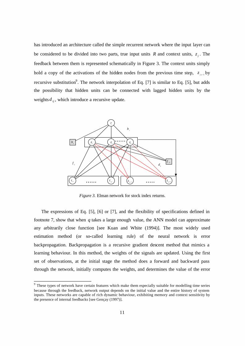
has introduced an architecture called the simple recurrent network where the input layer can

be considered to be divided into two parts, true input units R and context units, jz . The

feedback between them is represented schematically in Figure 3. The context units simply

hold a copy of the activations of the hidden nodes from the previous time step, 1, −tjz by

recursive substitution9. The network interpolation of Eq. [7] is similar to Eq. [5], but adds

the possibility that hidden units can be connected with lagged hidden units by the

weights ijδ , which introduce a recursive update.

jβ

1z2

z0

β

1,1 −tz

qz

j0φij

φij

δ

tr

1−tr ptr

− 1, −tqz

......

...... .....

Figure 3. Elman network for stock index returns.

The expressions of Eq. [5], [6] or [7], and the flexibility of specifications defined in

footnote 7, show that when q takes a large enough value, the ANN model can approximate

any arbitrarily close function [see Kuan and White (1994)]. The most widely used

estimation method (or so-called learning rule) of the neural network is error

backpropagation. Backpropagation is a recursive gradient descent method that mimics a

learning behaviour. In this method, the weights of the signals are updated. Using the first

set of observations, at the initial stage the method does a forward and backward pass

through the network, initially computes the weights, and determines the value of the error

9 These types of network have certain features which make them especially suitable for modelling time series because through the feedback, network output depends on the initial value and the entire history of system inputs. These networks are capable of rich dynamic behaviour, exhibiting memory and context sensitivity by the presence of internal feedbacks [see Gençay (1997)].

12

function, recomputes the weights, and redetermines the value of the error the target values

of the output variable. At the next stage, it uses the second set of observations, and so on.

This estimation procedure is characterized by the recursive process. The learning algorithm

converges and thus the process stops when the value of the error function is lower than a

predetermined convergence criterion.

More specifically, the network weight vector θ is chosen to minimize the sum of the

squared-error loss:

[ ]∑=

−T

ttt rr

1

2ˆmin

θ,

where T is the sample size, and tr is the calculated output value from Eq.[5], Eq.[6] and

Eq.[7]. Then the iterative step of the gradient descent algorithm takes θ to θθ ∆+ , and

( ) tttRf εθηθ ˆˆ,∇−=∆ ,

where η is the “learning rate”; ( )ttRf θ,∇ is the gradient of ( )ttRf θ, with respect to θ (a

column vector of parameters); and rtt rr ˆˆ −=ε is the “network error” between the computed

output and the target return value, tr . For recurrent networks, the network output depends

on θ directly and indirectly through the presence of lagged hidden-unit activations. For this

reason, the model can be estimated by the recurrent backpropagation algorithm and by the

recurrent Newton algorithm [see Gençay (1997) for details].

3. Data and preliminary statistics

This study uses the daily closing prices of the Spanish Ibex-35stock index, from 30

December 1989 to 10 February 2000, with a total of 2520 observations. The Ibex-35 index

(It) comprises the 35 most liquid values negotiated in the continuous system which during

the control period had the highest trading volume in cash pesetas. The Ibex-35 is a

composite index which is highly representative and is fitted by capitalisation and dividends

of the assets included, but not by expansions in capital. The series is transformed into

logarithms to compute continuous returns, according to the following expression:

=

−1

logt

tt I

Ir , where log is the natural logarithm.

13

Figure 4 shows the evolution of the index and its daily returns. Its sharp increase since

1996 is due to the downturn in risk- free interest rates and the sequential move by investors

towards the stock market. The period of special interest for the evolution of prices and

returns is the Asiatic crisis of 27-29 October 1997, when returns fell abruptly.

Figure 4. Time evolution of daily closing Ibex35 and returns. (i) Closing prices(ii) Returns

We study some statistical properties of the Ibex35 index, shown in Tables AI.1, AI.2

and AI.3 (see Appendix I). Table AI.1 reports the augmented Dickey-Fuller (ADF) and

Phillips and Perron (PP) statistics for non-stationarity for the logarithm index and returns.

The statistics indicate that log It is non-stationary and that the index of returns is stationary.

Another statistical test for the null hypothesis of stationarity, Kwiatkowski, Phillips,

Schmidt and Shin (KPSS), obtains the same results. Table AI.2 reports the variance-ratio

test. The results show the existence of negative autocorrelations or mean reversion (for

values between 452 ≤≤ q days). This test rejects the null hypothesis of random walk at the

10% significance level. Finally, the Table AI.3 reports the Brock, Dechert and Scheinkman

(BDS) test. This test indicates the presence of non-linearities and, therefore, of complex

models in the data10. The main conclusion is that Ibex35 stock index returns may be

predicted using non- linear models.

10 In order to avoid possible rejections of the null hypothesis due to non-stationarity the BDS test is commonly applied to the estimated residuals of the ARIMA process. The asymptotic distribution of BDS is not affected when linear filters are applied to data. Table AI-3 also shows “shuffled” residuals, i.e., recreated randomly as if they were “sample” data without replacement. We use this technique following Scheinkman and LeBaron (1989) in order to reinforce the results, so that in this case we should not reject the null

0

2000

4000

6000

8000

10000

12000

14000

9/1/92 14/1/94 22/1/96 16/1/98 14/1/00-0.12

-0.08

-0.04

0.00

0.04

0.08

9/1/92 14/1/94 22/1/96 16/1/98 14/1/00

14

4. Non-linear model estimates

The BDS statistic reveals considerable evidence of non- linearity, and the variance ratio

test shows that mean reversion exists. In this section, we analyse the non-linear model

estimates from the STAR and ANN models, which we consider to represent some stylised

facts of the short-term dynamics of stock index returns. The fitted period is 30 December

1989 to 30 April 1999 (T=2320 observations). We did not include GARCH models in the

set of forecasting models because these models parameterise the conditional variance,

whereas the object to be forecast is the stock index returns, not their volatility. However,

we tested for any omitted ARCH non- linearity.

4.1. STAR Models

This section investigates empirical issues regarding STAR models with Gaussian errors.

In this paper we do not distinguish between regimes of low and high volatility, because our

aim is to analyse stock index returns, not their volatility. Therefore, we evaluated different

models that show regime switching, for example, Eq. [2] with the ESTAR and LSTAR

function11. The modelling procedure for building STAR models is carried out in three

stages [see Granger and Teräsvirta (1993, pp.113-124), Teräsvirta (1994), and Eitrheim and

Teräsvirta (1996)]. The first stage is to specify a linear AR(p) model. We estimated

different AR models and chose p on the basis of the AIC, SBIC and Ljung-Box (LB)

statistics for autocorrelation. The AR model has a relatively short order. We chose p=2 on

the basis of AIC and SBIC equal to -5.92 and LB(1)=0.0 (P-value is 1.0), LB(5)=-0.001 (P-

value is 0.98) and LB(10)=0.039 (P-value is 0.78), which indicates that the AR(2) model

has white noise residuals. The second stage is to test the linearity against STAR models,

hypothesis of the i.i.d. linear process. Thus, we will be able to prove that there is a non-linear structure in the original data which has been removed by the “shuffling”. In both situations, we use m=2 to 8 and a value for ε between 0.5 σ and 2σ, using σ=0.1088. The results show that there are non -linear structures in data in the logarithm of the Ibex35 index, since the tests applied to residuals and to “shuffled” residuals show the rejection of the null hypothesis in the first case and its non-rejection in the second case. 11 Also, STAR models have been estimated assuming conditional heteroscedasticity or GARCH errors, but the results are worse than those obtained without considering such an assumption. For this reason, we have not shown it. Lundbergh and Teräsvirta (1998) made an extensive study of STAR models with GARCH errors.

15

for different values of the delay parameter d, using the linear model specified at the first

stage. This stage tests the parameter constancy, such as testing whether STAR is more

appropriate than a single AR model. Therefore, we tested whether non- linear functions of

lagged regressor variables contribute significantly to the fit (after correction for a linear AR

part), using dtt rs −= . The linearity test is based on the auxiliary regression:

∑ ∑∑∑= =

−−=

−−−−=

− +++++=p

j

p

jtdtjtj

p

jdtjtjdtjtj

p

iitit vrrrrrrrr

1 1

33

1

221

1110 βββφφ

To specify the value of the delay parameter d, the estimation of the auxiliary regression is

carried out for a wide range of values, Dd ≤≤1 , given uncertainty about the most

appropriate value of d. The null hypothesis is jiij ,,0 ∀=β . The F-test values for the

significance of the regressor added to the linear AR regressions can be used to test the null

hypothesis of linearity. We can obtain a first impression of the d value by looking at the

relative value of the F-test statistics, that is, the d for which the corresponding P-value is

smallest may be selected, and this corresponds to the largest 2R of the regression model. In

carrying out linearity tests, we considered values for the delay parameter over the range

121 ≤≤ d (Table 1). The d value selected is 6, because it has the lowest P-value. The

linearity is rejected at the 5% level of significance because the minimum P-value is

0.000001.

Table 1. P-values for linearity test and sequential procedure. Linearity test Choosing between ESTAR and LSTAR Delay 0: 3210 === βββH 0: 301 =βH 00: 3202 == ββH 00: 32103 === βββH 1 2 3 4 5 6 7 8 9 10 11 12

0.000017 0.003785 0.000155 0.001467 0.21942 0.000001ª 0.00608 0.00194 0.0005 0.0004 0.1787 0.0116

0.05234 0.6991 0.3504 0.001320 0.89108 0.000004b 0.004892 0.05794 0.05888 0.60798 0.02942 0.8671

0.000003 0.000221 0.00009 0.2169 0.8022 0.03413 0.04378 0.000930 0.02621 0.3756 0.8538 0.2582

0.7227 0.4296 0.04344 0.07367 0.02238 0.02762 0.5614 0.5462 0.00355 0.000017 0.4638 0.0012

Note: a indicates lowest P-value for the null hypothesis of linearity over the interval 120 ≤≤ d . b indicates lowest P-value when d=6.

16

The third stage is to choose between ESTAR and LSTAR models where linearity is

rejected. Teräsvirta (1994) suggests applying the following sequence of nested tests: (i) test

whether all fourth-order terms are insignificant, jj ∀= ,03β ; (ii) conditional on all fourth-

order terms being zero, test the joint significance of all third-order terms

jjj ∀== ,00 32 ββ , and (iii) conditional on all third and fourth-order terms being zero,

test the significance of the second-order terms, jjjj ∀=== ,00 231 βββ . If the test in (i)

does not reject the null hypothesis, we choose the LSTAR model. If we accept (i) and reject

(ii), we choose the ESTAR model. Finally, accepting the null hypothesis in (i) and (ii), but

rejecting (iii), we can choose an LSTAR model. We used P-values for the F-tests and made

the choice of the STAR model on the basis of the lowest P-value. The P-values obtained

were (i) 0.00004, (ii) 0.0341 and (iii) 0.02762. Thus, we chose to fit an LSTAR model

(Table 1).

The next step is to estimate the parameters in the STAR models. Table 1 summarises

the estimation results, including the ESTAR model. We used the MLE and BFGS

numerical algorithms, which satisfy various regularity conditions (such as stationary,

ergodicity, consistency and asymptotic normality). We now comment on some specific

aspects of the two models, although the model selected was LSTAR in terms of the

sequential procedure suggested by Teräsvirta (1994)12. The estimated coefficients are lower

than unity, jiij ,,1 ∀<φ . The ML estimations of the STAR model parameters of the two

regimes are similar. The t-statistics, reported in Table 2, are adjusted for heteroskedasticity

using White heteroskedasticity-consistent standard errors to assess the significance of the

parameter estimates.

With respect to the smoothness parameter (γ),this is always positive, small in the case

of ESTAR and large in the case of LSTAR. The LSTAR estimation suggests that regime

shifts or transitions between the regimes are smooth.

12 In general, the LSTAR and ESTAR models have the same number of parameters, and the comparison of their log-likelihoods may be meaningful. In this sense, the results show that both estimations are possible but, statistically, LSTAR(2;3) seems to fit better than ESTAR(2;3), in terms of the log-likelihood value. However, similar likelihood values might suggest that these models are likely to produce a similar forecast performance.

17

Table 2. MLE (BFGS) for STAR models. Period from 30-12-1989 to 30-04-1999. T=2350.

10φ 11φ 12φ 20φ 21φ 22φ γ c LogL

ESTAR 0.059 (1.26)

0.1801 (15.5)

-0.015 (-1.10)

-0.033 (0.32)

-0.1214 (-4.99)

-0.049 (1.76)

1.869 (2.11)

0.00159 (0.59)

-1685.0

LSTAR 0.044 (1.72)

0.1265 (13.01)

-0.015 (-1.29)

0.0435 (0.81)

-0.0423 (-1.77)

-0.1754 (5.74)

7.345 (1.75)

0.01214 (7.84)

-1683.1

Note: The t-Student values for the null hypothesis that the parameter is equal to zero are given in parentheses. These values are calculated using White heteroskedastic-consistent standard errors.

The regime shift or threshold parameter (c) indicates the halfway point between the

expansion and contraction regimes. This is positive and statistically significant at the 5%

level of significance in the ESTAR model and at 10% in the LSTAR model. Both models

are in the range of the transition variable 6−= tt rs (which varies between about -0.06 and

0.06). The transition is slow at the values for tr of c , with transition probabilities

( )csF tt ˆ,ˆ;ˆ6, γ switching from 0 to 1 at this point. The two regimes can be described as

follows: when 0=F , which we might refer to as the lower regime in the LSTAR model

and the middle regime in the ESTAR model, the mean process for tr is an AR(2) with

complex roots (i.e. for the ESTAR model i08.009.0 ± , having a modulus of 0.12; and for

the LSTAR model it is i22.0006.0 ±− with a modulus equal to 0.22). When 1=F , we

might refer to it as the upper or expansion regime in the LSTAR model and the outer

regime (expansion and contraction regime) in the ESTAR model. In this case, the mean

process for tr is also an AR(2) with complex roots (i.e. for the ESTAR model i10.006.0 ±

having a modulus of 0.12; and for the LSTAR model it is i42.0021.0 ±− with a modulus

equal to 0.42). So, if 6−tr exceeds 0.00159 in the ESTAR model and 0.01242 in the LSTAR

model, ( )csF tt ˆ,ˆ;ˆ6, γ can take values close to one, but with different dynamic properties.

Figure 5a shows the graph of ( )csF tt ˆ,ˆ;ˆ6, γ versus time in days, and Figure 5b displays

( )csF tt ˆ,ˆ;ˆ6, γ versus 6−tr for the ESTAR model. In this model, high values for the transition

probabilities imply that stock index returns are either in an expansion or in a contraction

regime (outer regime). From Figure 5b we observe that the behaviour of stock index returns

in the transition period or middle regime is different, but that the two regimes have similar

dynamics. In this sense, we cannot identify expansionary and contractionary phases, but we

can distinguish between the outer regime and the middle regime. Figures 6a and 6b show

18

the same relationships when the model is LSTAR. In this model, the cyclical behaviour of

stock returns can be inferred from the estimates of transition probabilities. When the

( )csF tt ˆ,ˆ;ˆ6, γ transition probabilities are greater than 0.5, the stock market could be

considered to be in an expansion regime. Figure 6a shows the probability of an expansion

regime ( )csF tt ˆ,ˆ;ˆ6, γ . We can clearly observe the periods of high and low returns and, from

Figure 6b, we see that the transition between high and low returns (expansion and

contraction regimes) is reasonably smooth, although there are not many data points for

which 6−tr exceeds c .

0.0

0.2

0.4

0.6

0.8

1.0

500 1000 1500 2000

Figure 5a. ( )csF tt ˆ,ˆ;ˆ6, γ ESTAR versus time.

0.0

0.2

0.4

0.6

0.8

1.0

-0.10 -0.05 0.00 0.05 0.10

Figure 5b. ( )csF tt ˆ,ˆ;ˆ6, γ ESTAR vs. 6−tr .

0.0

0.2

0.4

0.6

0.8

1.0

500 1000 1500 2000

Figure 6a. ( )csF tt ˆ,ˆ;ˆ6, γ LSTAR versus time.

0.0

0.2

0.4

0.6

0.8

1.0

-0.10 -0.05 0.00 0.05 0.10

Figure 6b. ( )csF tt ˆ,ˆ;ˆ6, γ LSTAR vs. 6−tr .

19

To evaluate the within-sample performance of the estimated STAR mode ls, we used

some misspecification tests, only for the LSTAR model. We did not use the Ljung-Box test

for serial correlation because simulation studies suggest that 2χ asymptotic distribution

may not be valid. Methods of testing the adequacy of fitted STAR models are discussed in

Eirtheim and Teräsvirta (1996). These authors contribute to the evaluation stage of a

proposed specification, estimation and evaluation of these models. To determine whether

such a model is adequate, we first tested the hypothesis of no error autocorrelation or serial

independence, but we did not reject the null hypothesis at the 5% level of significance.

Secondly, to test against general neglected non- linearity or remaining linearity, second and

third-order terms of the form jtit rr −− for i=1,..,p and j=i,...,p, and ktjtit rrr −−− for k=j,..,p may

be added to the LSTAR model and tested for significance. Doing so for the fitted

LSTAR(2;3) model leads to a statistic that is significant at any level (P-value equal to

0.00), which confirms the possibility of additive non-linearity, although a rejection as such

in general does not give much orientation as to what to do next [see Eitrheim and Teräsvirta

(1996)]. In this sense, if the non- linearity is manifests in the conditional variance, then we

would expect to find significant ARCH effects. Using the Lagrange multiplier test for

ARCH effects, we obtained a P-value that suggested the presence of this type of non-

linearity (i.e. ARCH(1) Lagrange Multiplier test with P-value equal to 0.00, ARCH(5)

equal to 0.00 and ARCH(10) equal to 0.00).

Another important assumption is test parameter constancy. Eitrheim and Teräsvirta

(1996) postulate a parametric alternative parameter constancy in STAR models, which

explicitly allows the parameters to change smoothly over time. These tests are monotonic

parameter change, a symmetric non-monotonic change and a more flexible test that allows

monotically and non-monotonically changing parameters. For these tests, the P-values are

0.5335, 0.9521 and 0.3564, respectively. In none of the three cases do we reject the null

hypothesis at the 5% level of significance.

Thus, the validity of the LSTAR model for stock returns depends on the existence of

remaining non-linearity and ARCH errors. We treat these empirical facts by reducing the

magnitudes of extreme observations and outliers, and explore the estimation of the MLE for

GARCH and STAR-type models by using two highly flexible non-linear models, namely

STAR-GARCH and STAR-Smooth Transition GARCH [see Lundbergh and Teräsvirta

20

(1998)]. These authors have extended the STAR model by incorporating the concept of

smooth transition into the GARCH component (STGARCH). This model is non- linear not

only in the conditional mean, but also in the conditional variance. Moreover, tε is assumed

to follow a GARCH(1,1) process that is useful for capturing volatility clustering, while the

threshold variables are useful if the data exhibit regime switching behaviour for varying

stock returns and tε . In the case of STGARCH-type models, we consider ( )epH t ,;ξ as a

transition function which satisfies the same conditions as ( )csF tdt ,;, γ . We assume there

exist two regimes with the transition variable 1−= ttp ε ; ξ is the transition rate; e is the

threshold value, and regarding the choice of transition function, we employ the first-order

logistic function. The following implications follow from the estimates in the LSTAR-

GARCH(1,1) and LSTAR-STGARCH(1,1) models. First, the MLE is extremely sensitive

to the choice of initial values. Second, convergence is achieved after very iterations. In the

case of LSTAR-GARCH(1,1), it is easily achieved but the transition variable selected for

the mean process is 2−tr . The estimated coefficients 4.31ˆ =γ and 03.0ˆ =c are significant

at the 5% level of significance, but the AR(2) parameters are not significant at any level.

The GARCH coefficients meet the sufficient conditions for strict positive conditional

variance ( 003.0ˆ =ω , 11.0ˆ1 =α and 82.01 =β , respectively). However, the results for the

LSTAR-STGARCH(1,1) model appear to be worse after such adjustments.

We conclude that the estimated models based on adjusted data perform similarly and do

not improve on the within-sample estimates in Table 2 for stock index returns. Although

the effects of misspecification of non- linear models are generally unknown, it is difficult to

draw firm conclusions about the effects of outliers and remaining non-linearity, because

there are difficulties in fitting the LSTAR-STGARCH model for two regimes.

4.2. Artificial neural network models

In this section we employ the technique of ANN estimation to obtain out-of-sample

forecasts. An important feature of ANNs is that they are non-parametric models. We do not

want to treat the ANN as a “black box”, in the sense that no analysis of the characteristics

21

and properties of the estimated networks is performed and no explanation is given as to

why these models perform quite well in the forecasting exercise.

The specific types of ANN estimated in this study are MLP(p,q), JCN(p,q) and

Elman(p,q) as discussed in Section 2. The architecture of these models includes one hidden

layer and various hidden units or elements of the single hidden layer (q). The output

variable is the daily stock return. The input variables selected in the input layer include

lagged stock index returns, p (the number of lags in the autoregressive part), and are scaled

assuming a uniform distribution within the interval [-1;1]. The p-order lagged returns are

calculated by sequential validation, and so we estimate ANN models with different values

of p and q. The rank of the terms employed is p,q=1,…,5. The inclusion of these lags is

based on the evidence in Section 4.1 that suggests lagged returns are needed in the

conditional mean specification, while autocorrelation in the stock index returns can appear

because of non-synchronous trading effects. Moreover, a link was introduced between the

input variables and the output variable. As there is no reliable method of specifying the

optimal number of hidden layers, we specified one hidden layer. This choice was made

because many studies that carry out sensitivity analysis to determine the optimal number of

hidden layers have found that one hidden layer is generally effective in capturing non-linear

structures [see Adya and Collopy (1998) for an overview]. The hidden unit activation

function g(.) is the hyperbolic tangent function [see footnote 7], because it produces a better

fit. We did not choose p, q and g(.) a priori.

The ANN models were trained over a training period (i.e. training sample) using 1500

training cycles and crossvalidation. The training set was used to estimate the neural

network weights. To improve on the in-sample fitting performance of the ANN models, the

estimated set of weights was used as a set of initial values for training. We used cross-

validation strategy in training to avoid overfitting (good in-sample, but poor out-sample

performance). The training phase of the ANN was performed with 1855 observations,

whereas in the “test” phase 463 observations were used, both sizes being randomly

determined. The two hundred final observations were set aside to make predictions. The

decrease in the error rate in the training and “test” phases was then tested. The output was

compared to the sample of original values of the output by comparing the root mean

squared error (RMSE). We observed as the RMSE declines over successive training (i.e.,

22

n). When RMSE reaches a minimum and then starts increasing, this indicates that

overfitting may occur. On the basis of the estimated weights from n-th training over the

training period, out-of-sample forecasts were generated for subsequent “test” periods.

Table 3. MSE and MAE statistics of the ANN models with a single hidden layer during the training phase (period from 30-12-1989 to 17-06-97) and the “test” phase (period from 18-06-1999 to 30-04-99).

MLP(p,q) JCN(p,q) Elman(p,q) Training Test Training Test Training Test p q MSE MAE MSE MAE MSE MAE MSE MAE MSE MAE MSE MAE 1 1 15.04 3.735 17.39 3.852 1.220 0.805 3.313 1.373 15.18 3.753 17.53 3.869 2 1.598 0.915 3.937 1.503 1.268 0.825 3.419 1.343 1.384 0.881 3.470 1.388 3 1.220 0.804 3.309 1.372 1.602 0.923 4.090 1.566 1.210 0.803 3.287 1.357 4 1.194 0.800 3.219 1.328 1.183 0.793 3.218 1.334 1.204 0.799 3.249 1.356 5 1.241 0.811 3.371 1.392 1.185 0.795 3.213 1.326 1.186 0.795 3.208 1.332 2 1 1.895 1.078 3.873 1.458 1.250 0.821 3.398 1.340 2.167 1.178 4.130 1.523 2 1.307 0.830 3.726 1.440 1.198 0.800 3.195 1.322 3.195 1.247 9.849 2.193 3 1.209 0.805 3.333 1.335 2.539 1.198 5.864 1.764 1.186 0.794 3.193 1.332 4 1.119 0.798 3.202 1.318 1.218 0.803 3.235 1.322 1.190 0.797 3.205 1.325 5 1.323 0.838 3.708 1.439 1.184 0.794 3.237 1.337 1.183 0.793 3.227 1.332 3 1 2.752 1.391 4.936 1.785 1.477 0.891 4.144 1.516 2.395 1.273 4.573 1.698 2 1.653 0.996 3.772 1.498 1.541 0.905 3.838 1.447 1.772 1.045 3.897 1.532 3 1.182 0.793 3.232 1.332 1.185 0.794 3.214 1.338 1.183 0.796 3.183 1.324 4 1.350 0.846 3.858 1.461 1.213 0.803 3.345 1.365 1.260 0.818 3.590 1.411 5 1.180 0.792 3.205 1.327 1.182 0.792 3.201 1.326 1.424 0.870 3.595 1.371 5 1 1.190 0.796 3.249 1.344 2.304 1.193 5.020 1.683 1.181 0.793 3.224 1.330 2 2.620 1.352 4.759 1.752 1.570 0.914 4.258 1.548 1.945 1.114 4.060 1.579 3 1.413 0.869 3.845 1.452 1.280 0.831 3.546 1.397 1.188 0.796 3.314 1.353 4 1.594 0.917 4.497 1.544 1.538 0.907 4.257 1.512 1.292 0.836 3.666 1.409 5 1.422 0.861 3.987 1.490 1.178 0.793 3.225 1.330 1.196 0.798 3.209 1.322 Note: Bold type denotes the MAE and MSE in the training and test phases which correspond to the best MSE in the out -of-sample phase.

Table 3 shows the final results in the training and “test” phases in the last iteration for

mean squared error (MSE) and mean absolute error (MAE) statistics. The estimates of

network patterns present the following aspects. In terms of the minimum MSE in the out-

of-sample phase, the best adjusted model holds two-explanatory variables, p=2 (i.e. the

one-period and two-period lagged stock index returns, 1−tr and 2−tr , as ESTAR and LSTAR

estimated models in Section 4.1), and q=4 hidden units in the single hidden layer in Eq. [5]

and Eq. [6], and q=3 in Eq. [7]. We can write these models as MLP(2,4), JCN(2,4) and

23

Elman (2,3) artificial neural networks. For these selected models, the MLP model has a

lower MSE and MAE than the JCN and Elman models in the training phase (within-

sample). If we compare the ANN results with the AR and STAR models, the ANN models

fit the within-sample data better than the other models (i.e. regarding the MSE and MAE

statistics, AR(2) has 1.526 and 1.098; ESTAR(2;3) has 1.173 and 0.791; and LSTAR(2;3)

has 1.171 and 0.788).

We do not report the estimated weights from training the ANN model given in Eq.[5],

Eq.[6] and Eq.[7] for the training period. However, there are some similarities regarding the

magnitudes and signs of the weights that appear in all these models, such as jijj ,00ˆˆ,ˆ,ˆ φφββ ,

i=1,…,p, j=1,..,q.

Let us consider what kind of non- linear relationships between the return and past

returns are picked up by ANNs. Like Qi and Maddala (1999), to visualize what relationship

between returns and the underlying predicting variables has been captured by the neural

network, we report the results of sensitivity analysis and compare it with the observed

returns. As an illustrative graph of possible non-linearity, let us consider Figure 7, which

plots the observed returns ( tr ) against the one-period lagged return ( 1−tr ) and the two-

period lagged return ( 2−tr ) in three samples: (i) the first sample is similar to the training set;

(ii) the second is similar to the “test” phase; and (iii) the third is equivalent to the forecast

phase. Figure 8 contains various groups of graphs (Figures 8a, 8b and 8c), which show the

estimated returns in the training, “test” and forecast phases from the neural network for

MLP (Figure 8a), JCN (Figure 8b) and Elman (Figure 8c) aga inst the observed 1−tr and

2−tr . In Figures 8a, 8b and 8c, case (c) plots the simulated stock return ( tr ) from the neural

network for MLP, JCN and Elman in the forecast phase against 1−tr and 2−tr . From these

graphs, we can observe a complex non- linear relationship between returns and lagged

returns, showing that this series displays a cyclical behaviour around points that shift over

time when these shifts are endogenous, i.e., caused by past observations on tr themselves,

which can be viewed as a typical feature of non-linear time series. MLP and Elman ANNs

perform better than JCN.

24

Figure 7. Observed returns.

(i) First sample (ii) Second sample (iii ) Third sample

Figure 8. Sensitivity analysis

Figure 8a. MLP(2,4) estimated returns and lagged observed returns.

(a) Training (b) Test (c) Forecast

Figure 8b. JCN(2,4) estimated returns and lagged observed returns.

(a) Training (b) Test (c) Forecast

25

Figure 8c. Elman(2,3) estimated returns and lagged observed returns.

(a) Training (b) Test (c) Forecast

The better fit of the neural network model reported above is not surprising given its

universal approximation property.

5. Statistical assessment of the out-of-sample forecast

This section focuses on the out-of-sample forecasting ability of the STAR and ANN

models in terms of statistical accuracy. The randomly selected prediction period

corresponds to the last 200 periods of the sample. This forecast period was from 3 May

1999 to 10 February 2000. One-step-ahead forecasts were generated from all models.

It is generally impossible to specify a forecast evaluation criterion that is universally

acceptable. In order to assess the predictive ability of the different models, we use various

statistics of prediction accuracy. The measures of accuracy used in this paper are based on

h=1,...,H prediction periods for rh, called hr . Although ANN is expected to have a superior

in-sample performance, since it nests the AR linear model and STAR model, there is no

guarantee that it will predominate in the out-of-sample period. The relationship between

stock returns and lagged stock returns was investigated by comparing the predictions of AR

and non-linear models that can be used for return prediction.

The forecast evaluation was made between the results from the following models for

stock index returns: AR(2), LSTAR(2;3), ESTAR(2;3), MLP(2,4), JCN(2,4), and

Elman(2,3), strictly for the prediction period. We did not include GARCH models in the set

of forecasting models because these models parameterise the conditional variance, whereas

the object to be forecast is the stock index returns, not its volatility.

26

We compared the out-of-sample forecasts using two different testing approaches. First,

we examined the forecast accuracy from all the estimated models by calculating the MAE,

mean absolute percentage error (MAPE), RMSE, U-Theil and the proportion of times the

signs of returns are correctly forecasted (Table 4, Panel A). In terms of classic forecast

evaluation criteria, the best results are the lowest values. As indicated in this table, the

MAE, RMSE and U-Theil of the forecasts from the ANN models are lower than those of

the linear model, except in the Elman net for RMSE. In terms of MAPE, AR is better than

the other models. However, the signs correctly estimated are slightly superior in ANNs,

with 55% success in the MLP model. This result implies that the ANN-based forecasts are

in general more accurate than those of the linear and STAR models.

Second, to examine the directional prediction of changes, the forecast encompassing

and to analyse whether the difference between the RMSEs is statistically significant for our

out-of-sample forecasts, we employed various tests of hypotheses, such as the Pesaran and

Timmermann (DA, 1992) test, which was used as a directional prediction test of changes.

Under the null hypothesis, the real and predicted values are independent. The distribution

of the DA statistic is N(0,1), and it has the following structure:

( ) ( )[ ] ( )SRISRSRISRDA −−= − 5.0varvar , where [ ]∑=

− >=H

hhhi yyIHSR

1

1 0ˆ. and

( )( )1111 ˆ11ˆ ppppSRI −−+= , where SRI is the success ratio in the case of independence

between the real and predicted values under the null hypothesis. The other elements

are: [ ]∑=

− >=H

hhi yIHp

1

11 0 , [ ]∑

=

− >=H

hhi yIHp

1

11 0ˆˆ , ( ) ( )[ ]SRISRIHSR −= − 1var 1 and

( ) ( ) ( ) ( ) ( ) ( )( )[ ]1111112

1112

12 ˆ11ˆ4ˆ1ˆ1211ˆ2var ppppppppppHHSRI −−+−−+−−= − . The

results are reported in Table 4, Panel B. At the 5% significance level these results do not

reject the null hypothesis that forecasts and realizations are independent, which indicates

that independence is not rejected for all the linear and non-linear models analysed.

We employed the forecast encompassing testing approach for our out-of-sample

forecasts. In forecast encompassing, the criterion is that the i-th model should be preferred

to the j–th model if the former can explain what the latter cannot. Let ( )jtit ff , be two

competing forecasts of stock returns. When itf encompasses tf2 , Chong and Hendry (1986)

27

and Clements and Hendry (1993) refer to this concept as “forecast conditionally

efficiency”. The encompassing test of Chong and Hendry (1986) explores the

encompassing forecast. To illustrate this, let ie be the forecast error for model i and je the

forecast error from model j (i,j=AR, ESTAR, LSTAR, MLP, JCN and Elman). Given

forecasts from these models, we can test the null hypothesis that neither model

encompasses the other by running two regressions: the first involves regressing by ordinary

least squares (OLS) the forecast error from the i-th model on the difference of forecasts

between two models. Then, the equation to be estimated is:

( ) hjhihih ueee +−+= 11 λα ,

thus obtaining the estimated coefficient 1λ . The second involves the regression of the

forecast error from the j-th model on the difference of forecasts:

( ) hjhihjh ueee +−+= 22 λα

and obtaining the estimated coefficient 2λ (13).

The results appear in Table 4, Panel C. In this panel, we also consider the prediction

error of the random walk, erw. In this case, we want to know if the prediction of the i-th

model includes or is conditionally more efficient than the prediction of the random walk.

This panel reports the t-statistics of the estimated coefficients and P-values in brackets. In

this case, the standard regression-based statistic for testing the null hypothesis is corrected

by using the Harvey, Leybourne and Newbold (1998) correction, because these authors

have shown that the tests of forecast encompassing and equality of MSE (like the Diebold

and Mariano test) are affected by the non-normality of forecast errors.

13 Applying the standard regression-based test of the null hypothesis λ1=0 and λ2=0, if 1λ is not statistically

significant and 2λ is statistically significant, then we reject the null hypothesis that neither model encompasses the other in favour of the alternative hypothesis that the i-th model encompasses the j-th model. If 1λ is significant and 2λ is not significant, then the j-th model encompasses the i-th model. If both 1λ and

2λ are significant or if neither are significant, then we fail to reject the null hypothesis that neither model encompasses the other.

28

Table 4. Forecast evaluation. Statistical criteria for the linear and non- linear stock return models. Period from 3-05-1999 to 10-02-2000. H=200.

RW AR ESTAR LSTAR MLP JCN Elman Panel A: Goodness of forecast

MAE MAPE RMSE U-Theil Signs

1.000

0.9042 112.77 1.1353 0.8821 0.505

0.9104 116.31 1.1417 0.8782 0.515

0.9049 115.22 1.1345 0.8750 0.515

0.9000 115.99 1.1309 0.8883 0.555

0.9014 116.90 1.1331 0.8779 0.534

0.9095 118.93 1.1410 0.8675 0.525

Panel B: Pesaran and Timmermann test DA 0.2066

[0.42] -0.3837 [0.65]

-0.0292 [0.51]

0.7677 [0.22]

0.01798 [0.49]

0.2162 [0.41]

Panel C: Chong and Hendry test Upper triangular matrix: 1λ and P-value

RW

AR

ESTAR

LSTAR

MLP

JCN

Elman

2λ

--

0.52 [0.0] 0.85 [0.0] 0.07 [0.0] -0.01 [0.0] -0.05 [0.0] -0.11 [0.0]

0.48 [0.40]

--

-2.87 [0.01] -0.18 [0.88] -0.10 [0.89] -0.44 [0.35] -1.45 [0.08]

0.14 [0.79] -1.87 [0.10]

--

0.88 [0.39] 0.38

[0.59] -0.19 [0.69] -0.25 [0.77]

0.53 [0.33] 0.82

[0.50] 1.88

[0.07] --

-0.20 [0.81] -0.48 [0.36] -1.13 [0.16]

0.86 [0.28] 0.89

[0.24] 1.38

[0.05] 0.80

[0.32] --

-1.15 [0..38] -0.93 [0.09]

0.57 [0.37] 0.56

[0.24] 0.81

[0.09] 0.52

[0.31] -0.15 [0.91]

--

-0.66 [0.09]

0.31 [0.50] -0.45 [0.58] 0.75

[0.38] -0.13 [0.87] 0.07

[0.89] 0.33

[0.39] --

Note: P-values appear between brackets. In the case of the Chong and Hendry test, the standard regression-based statistic for testing the null hypothesis is corrected by using the Harvey, Leybourne and Newbold (1998) expressions.

The upper triangular matrix of this panel shows t-statistics and P-values for 1λ and the

lower triangular matrix shows t-statistics and P-values for 2λ . If the P-values of both

estimated coefficients are lower than 5%, then the null hypothesis should be accepted (that

neither model encompasses the other). If the P-value of 1λ is lower than 5% and the P-value

of 2λ is higher than 5%, then the null hypothesis should be rejected in favour of the

alternative hypothesis that the i-th model encompasses the j-th model. Finally, if the P-

value of 1λ is higher than 5% and the P-value of 2λ is lower than 5%, the null hypothesis

is rejected in favour of the alternative that the j-th model encompasses the i-th model. For

example, as shown in Table3, Panel C, the null hypothesis is not rejected for all models.

When the i-th model is equal to an ANN model and the j-th model is an AR model, this

29

means that the ANN model explains the forecast error of the linear model, whereas the

linear model cannot explain the forecast error of the ANN. Also, comparing the random

walk and the other models, we do not always reject the null hypothesis for 1λ at any

significance level. In this sense, the prediction of the i-th model is conditionally more

efficient than the predic tion of the random walk.

Finally, we evaluated the equality of competitive forecasts by the Diebold and Mariano

(DM, 1995) test, which examines whether the difference in the RMSE of the forecasts of

the two models is statistically significant. Given two h-step-ahead predictors, and denoting

the corresponding prediction errors by e1h and e2h, then the null hypothesis is tested that

[ ] ( )hhhh eefddE 21 ,,0 == where dh is a function of the prediction errors. These authors

assume that the f(.) case is of the type ( ) ( )hhh egegd 21 −= . For example, if 22

21 hhh eed −= ,

the null hypothesis is that the two forecasts have an equal mean squared error. The

statistical test is based on the sample mean d . It is ( )[ ] ddVS2/1ˆ −

= , where ( )dV is a

consistent estimator of the variance of the sample distribution of d . The statistic has a

standard normal asymptotic distribution under the null hypothesis. The consistent estimator

is given by: ( ) ( ) ( )( )

,ˆ0ˆ2ˆ1

1∑

−

+−=

==k

kddfdV

τ

τγπ and ( ) ( )( )ddddH h

H

hhd −−= −

+=

− ∑ ττ

τγ1

1ˆ .

However, Harvey, Leybourne and Newbold (1997, 1998 and 1999) have shown that the

tests of forecast encompassing and the DM test are affected by non-normality of forecast

errors and by the presence of ARCH effects. In particular, under these circumstances the

tests are heavily oversized. Non-normality and ARCH are most likely to be important

properties of the forecast errors in the present application to daily stock index returns.

Hence, it would be useful to use the modified versions of the forecast evaluation tests

developed by Harvey et al. (1997, 1998 and 1999), which were designed to alleviate the

problem of size distortion.

Tables 5 and 6 show the corrected results of the Diebold and Mariano test (S) for the

assumptions that hhh eed 21 −= and 22

21 hhh eed −= , respectively. We consider 2e forecast

errors in columns and 1e in rows. The null hypothesis that 0=hd is rejected at the 5%

significance level in both cases. The sign of S is important. If 0<S , then 0<d , and so

the RMSE of model 1 is significantly smaller than that of the model 2 forecasts. On the

30

contrary, if 0>d , then the RMSE of model 2 is significantly smaller than that of the

model 1 forecasts. For example, if we use the random walk as 2e and use different forecast

errors as 1e (for example, AR2, ESTAR, LSTAR, MLP, JCN and Elman), we observe that

0<d in all cases. In this sense, the model considered as 1 always has a smaller RMSE

than the random walk. Another interesting result is that the ANN models are preferred to

the linear and STAR models, because the Diebold and Mariano test is positive. Also, the

MLP model is preferred to the JCN and Elman models, because when we consider MLP as

1e and JCN and Elman as 2e , we have 0<d .

Table 5. Diebold and Mariano test (S) with ttt eed 21 −= , for the linear and non-linear model of returns. Period from 3-05-1999 to 10-02-2000. H=200.

2e RW AR2 ESTAR LSTAR MLP JCN Elman RW -- 106.07 104.71 105.75 96.48 90.64 107.53 AR2 -106.07 -- -23.87 -2.03 6.82 2.34 -16.74 ESTAR -104.71 23.87 -- 14.77 15.67 9.01 2.17 LSTAR -105.75 2.03 -14.77 -- 8.14 3.20 -10.90 MLP -96.48 -6.82 -15.67 -8.14 -- -5.57 -11.69 JCN -90.64 -2.34 -9.01 -3.20 5.57 -- -7.02

1e

Elman -107.53 16.74 -2.17 10.90 11.69 7.02 -- Note: Critical distribution values N(0,1) are 1.645, 1.96, 2.576 at 10%, 5%, and 1%, respectively.

Table 6. Diebold and Mariano test (S) with 22

21 ttt eed −= , for the linear and non-linear

model of returns. Period from 3-05-1999 to 10-02-2000. H=200.

2e RW AR2 ESTAR LSTAR MLP JCN Elman RW -- 84.78 86.13 84.98 80.84 78.14 85.09 AR2 -84.78 -- -18.67 3.97 7.41 1.48 -25.68 ESTAR -86.13 18.67 -- 14.76 15.41 8.39 1.60 LSTAR -84.98 -3.97 -14.76 -- 5.17 0.23 -19.60 MLP -80.84 -7.41 -15.41 -5.17 -- -8.81 -13.75 JCN -78.14 -1.48 -8.39 -0.23 8.81 -- -7.36

1e

Elman -85.09 25.68 -1.60 19.60 13.75 7.36 -- Note: Critical distribution values N(0,1) are 1.645, 1.96, 2.576 at 10%, 5%, and 1%, respectively.

Thus, we conclude that in terms of classic forecast evaluation criteria, directional

prediction tests and MSE, the ANN prediction slightly improves on the results of linear AR

and STAR regime switching models.

31

6. Assessment the relative forecast performance with economic criteria in a simple trading strategy.

We must consider why ANN mode ls perform well in the forecasting exercise. In this

Section, we assess the economic criteria. We could use the return forecasts from the

different models in a simple trading strategy and compare the pay-offs to determine if

ANNs are useful forecasting tools for an investor. As shown by Leitch and Tanner (1991)

and by Satchell and Timmermann (1995), the use of statistical or economic criteria can lead

to very different outcomes. In fact, the correlation between MSPE and trading profits, for

example, is usua lly quite small, and the performance of a particular model in terms of DA

is often a better indicator of its performance in a trading strategy. Given that the present

paper finds that neural networks do not perform much better than linear and STAR models

in terms of DA, we would not find it surprising if it turned out that ANNs do not offer

significantly higher trading profits. Finally, it would also be useful to examine the impact

of transaction costs on the profits of trading strategies.

As pointed out by Satchell and Timmermann (1995), standard forecasting criteria are

not necessarily particularly well suited for assessments of economic value of predictions of

a non- linear process.

In order to assess the economic significance of predictable patterns in the Ibex-35

series, it is necessary to consider explicitly how investors may exploit the computed local

predictions as trading rules.

The trading rules considered in this paper are based on a simple market timing strategy,

consisting of investing total funds in either the stock market or a risk-free security. The

forecast from each predictor is used to classify each trading day into periods “in” (earning

the market return) or “out” of the market (earning the risk-free rate of return security). The

trading strategy specifies the position to be taken the following day, given the current

position and the “buy” or “sell” signals generated by the different predictors. On the one

hand, if the current state is “in” (i. e., holding the market) and the share prices are expected

to fall on the basis of a sell signal generated by one particular predictor, then shares are sold

and the proceeds from the sale invested in the risk- free security (earning the risk- free rate

of return ftr ). On the other hand, if the current state is “out” and the predictor indicates that

32

share market prices will increase in the near future, the rule returns a “buy” signal and then

the risk- free security is sold and shares are bought (earning the market rate of return ftr ).

Finally, in the other two cases, the current state is preserved (Fernández, Sosvilla and

Andrada, 2002).

The trading rule return over the predicted period of 1 to H can be calculated as:

+−

⋅+⋅+⋅= ∑∑== c

cnIrIrr sh

H

hfhbh

H

hh 1

1log

11

where hr is the market rate of return constructed over the closing price (or level of the

Ibex-35 stock index, hP ) on day h; bhI and shI are indicator variables equal to one when

the predictor signals are to buy and sell, respectively, and zero otherwise, satisfying the

relation [ ]HhII shbh ,1,0 ∈∀=⋅ ; n is the number of transactions; and c denotes the one-way

transaction costs (expressed as a fraction of the price). Regarding the transaction costs,

results by Sweeny (1988) suggest that large institutional investors could achieve in the mid-

1970s one-way transaction costs in the range of [0.1-0.2%]. Even though there have been

substantial reductions in costs in recent decades, we initially used one-way transaction costs

of 0.15%. We also investigated the robustness of the results with transaction costs of

0.25%.

In order to assess profitability, it is necessary to compare the return from the trading

rule based on the predictors to an appropriate benchmark. To that end, we constructed a

weighted average of the return from being long in the market and the return from holding

no position in the market and thus earning the risk- free rate of return. The return on this

risk-adjusted buy-and-hold strategy can be written as:

( )

+−

⋅+−+= ∑∑== c

crrr

H

hfh

H

hhbh 1

1log21

11

ββ

where β is the proportion of trading days that the rule is in the market.

In this paper we combine a simple and popular trading strategy known as the filter

technique, originally analysed by Alexander (1961) and Fama and Blume (1966), with

parametric and non-parametric forecasts, and compare the return obtained with this risk-

adjusted buy-and-hold strategy. In the empirical implementation, we modified the simple

rule by introducing a filter in order to reduce the number of false buy and sell signals, by

33

eliminating “whiplash” signals when one selected predictor at date t is around the closing

price at t-1 . This filtered rule will generate a buy (sell) signal at date t if the predictor is

greater than (is less than) the closing price at t-1 by a percentage δ of the standard

deviation σ of the return time series from 1 to t-1. Therefore, if hr denotes the prediction

for hr :

• If σδ ⋅+> −1ˆ hh rr and we are out of the market, a buy signal is generated. If we are

in the market, the trading rule suggests we should continue holding the market.

• If σδ ⋅−< −1ˆ hh rr and we are in the market, a sell signal is generated. If we are out

of the market, we continue holding the risk-free security.

We used a range filter percentage 0:0.025:0.3, because higher filters generate no

signals.

Table 7. Cost of 0.15%. Different filters. Statistics AR2 ESTAR LSTAR MLP JCN Elman

Panel A: Filter 0.0*σ r -0.00005 -0.00039 0.00009 0.00046 0.00005 -0.00002

bhr 0.00059 0.00059 0.00058 0.00070 0.00068 0.00055

arRS − -0.00714 -0.05518 0.01237 0.05190 0.00534 -0.00251 Panel B: Filter 0.3*σ

r 0.00096 0.00096 0.00096 0.00046 0.00123 0.00058

bhr 0.00052 0.00052 0.00052 0.00021 0.00062 0.00076

arRS − 0.15567 0.15567 0.15567 0.34451 0.16237 0.06010 Table 8. Cost of 0.25%. Different filters. Statistics AR2 ESTAR LSTAR MLP JCN Elman

Panel A: Filter 0.0*σ r -0.00058 -0.00095 -0.00052 0.00003 -0.00036 -0.00054

bhr 0.00058 0.00058 0.00057 0.00069 0.00067 0.00054

arRS − -0.08084 -0.13313 -0.07477 0.00366 -0.04248 -0.08338 Panel B: Filter 0.3*σ

r 0.00095 0.00095 0.00095 0.00045 0.00122 0.00055

bhr 0.00052 0.00052 0.00052 0.00020 0.00061 0.00075

arRS − 0.15403 0.15403 0.15403 0.33687 0.16104 0.05698

34

Given that individuals are generally risk averse, besides the excess return, we also

considered a version of the Sharpe ratio (Sharpe, 1966). This is a risk-adjusted return

measure given by:

*br

ar

rRS

σ=−

where r is the average return of the trading strategy and ** σβσ ⋅=br

is the proportion of

standard deviation of daily trading rule returns from being long in the market. As can be

seen, the higher the Sharpe risk-adjusted ratio, the higher the mean net return and the lower

the volatility returns from being long in the market.

The out-of-sample statistics with transaction costs of 0.15% and 0.25% are reported in

Tables 7 and 8, respectively. In both cases we used the filter technique with extreme filters

of 0.0% and 0.3% (Panels A and B, respectively)14 .

As can be seen in Panel A of Table 7, we find non-negative mean returns for the out-of-

sample period considered (except for the AR2, ESTAR, and ELMAN models). The MLP

model of artificial neural networks yields higher mean returns than all other models. The

results are similar in the Sharpe risk-adjusted ratio.

The introduction of the percentage band increases the spread between the number of

buy and sell signals generated by each model. As can be seen in Panel B, we also found

non-negative mean returns for the out-of-sample period considered, with all models. This

panel reveals a high Sharpe risk-adjusted ratio from the MLP model, even though this gives

the lower mean return. The results obtained show that the JCN model performs best.

These findings are similar to those given in Panel B of Table 8, but in Panel A we get

non-negative mean returns and the Sharpe risk-adjusted ratio for the out-of-sample period

was considered only for the MLP model.

In general, the filter techniques show that the MLP model improves on the mean returns

from parametric specifications, which are common in financial market returns, in nine of

the thirteen filters analysed. However, if we compare them with a risk-adjusted buy-and-

hold strategy, we get a higher mean return for filters higher than 0.125% with both

transaction costs.

35

7. Conclusions.

The present paper compares out-of-sample forecasts of daily returns for the Ibex-35

index, generated by six competing models, namely a linear AR model, the ESTAR and

LSTAR smooth transition autoregressive models and three ANN models: MLP, JCN and

Elman networks. We only considered the lagged returns as explanatory variables, because

we wanted to analyse the dynamic characteristics of returns from the stock index. The

comparison of out-of-sample forecasts was carried out on the basis of two approaches:

different statistical criteria and by assessing the economic value of the predictors. In terms

of the statistical criteria, we calculated various measures. First, we calculated the MAE,

MAPE, RMSE, U-Theil and the number of corrected signs predicted. Second, we used the

Pesaran and Timmermann test, and Chong and Hendry’s forecast encompassing test. Third,

we tested whether RMSE differences between the six competitors (and adding a random

walk model) are statistically significant. In all cases, the results suggest that the out-of-

sample ANN forecasts are more accurate than AR and STAR models. Furthermore, the

ANN forecasts can explain the forecast errors of the former models. For this reason, we

conclude that ANN models provide a better fit than the other models, and that MLP gives

the best values.

In terms of the economic criteria in the out-of-sample forecasts, we assessed

profitability by means of a simple trading strategy known as the filter technique, using a

range filter percentage and trading costs. The results indicate a better fit for the ANN

models, in terms of the Sharpe risk-adjusted ratio.

After assessing different statistical and economic criteria, we conclude that the return

on the Ibex-35 index can be predicted by using ANN models.

14 Complete results are available on request to the authors.

36

References Adya, M. and Collopy, F. (1998). “How Effective are Neural Networks at Forecasting and

Prediction?. A Review and Evaluation”. Journal of forecasting, 17, 481-495. Reference:

Alexander, S. (1961): “Price Movements in Speculative Markets: Trends or Random Walks”. Industrial Management Review, 2, 7-26.

Brock, W., Dechert, W. and Scheinkman, J. (1987): “A Test for Independence based on the Correlation Dimension”. University of Wisconsin, Dept. of Economics. Revised in Brock, W., Dechert, W., Scheinkman, J. and LeBaron, B. (1996), Econometric Reviews, 15, 197-235.

Campbell, J., Lo, A. and MacKinley, A. (1997): The Econometric of Financial Markets. Princeton University Press, Princeton, New Jersey.

Chong, Y. and Hendry, D. (1986): “Econometric Evaluation of Linear Macroeconomic Models”. Review of Economic Studies, 53, 671-690.

Clements, M. and Hendry, D. (1993): “On the Limitations of Comparing Mean Square Forecast Errors”. Journal of Forecasting, 12, 617-637.

Clements, M. and Hendry, D. (1998): Forecasting Economic Time Series. Cambridge, UK: Cambridge University Press.

Cochrane, J. (1988): “How Big is the Random Walk in GNP?”. Journal of Political Economy, 96, 893.920.

De Lima, P. (1998): “Non Linearities and Nonstationarities in Stock Return”. Journal of Business and Economic Statistics, 16(2), 227-236.

Diebold, F. and Mariano, R. (1995): “Comparing Predictive Accuracy”. Journal of Business & Economic Statistics , 13(3), 253-263.

Elman, J.L. (1990): “Finding Structure in Time”. Cognitive Sciencie 14, 179-211. Eitrheim, O and Teräsvirta, T. (1996): “Testing the Adequacy of Smooth Transition Autoregressive

Models”. Journal of Econometrics, 74, 59-75. Fama, E. and Blume, M. (1966): “Filters Rules and Stock Market Trading Profits”. Journal of

Business , 39, 226-241. Fama, E. and French, K. (1988): “Permanent and Temporary Components of Stock Prices”. Journal

of Political Economy, 96(2), 246-273. Fernández, F., Sosvilla, S. y García, D. (1997): “Using Nearest-Neighbour Predictors to Forecast

the Spanish Stock Market”. Investigaciones Económicas, 21, 75-91. Fernández, F., García, D. and Sosvilla, S. (1999): “Dancing with Bulls and Bears: Nearest-

Neighbour Forecast for the Nikkei Index”. Japan and the World Economy, 11, 395-413. Fernández, F., González, Ch. y Sosvilla, S. (2000): “On the Profitability of Technical Trading Rules

based on Artificial Neural Networks: Evidence from the Madrid Stock Market”. Economic Letters, 69(1), 89-94. Reference:

Fernández, F., Sosvilla, S. y Andrada, J. (2002). “Technical analysis in foreign exchange Markets: Evidence from the EMS” ,, forthcoming in Applied Financial Economics.

García, R. and Gençay, R. (2000): “Pricing and Hedging Derivative Securities with Neural Networks and a Homogeneity Hint”. Journal of Econometrics, 94, 93-115.

Gençay, T. (1996): “Non-Linear Prediction of Security Return with Moving Average Rules”. Journal of Forecasting, 15, 165-174.

Gençay R. and Liu T. (1997): “Nonlinear Modeling and Prediction with Feedforward and Recurrent Networks”. Physica D, 108, 119-134.

Granger, C.W.J. (1992): “Forecasting Stock Market Proces: Lessons for Forecasters”. International Journal of Forecasting, 8, 3-13.

37

Granger, C.W.J. and Teräsvirta, T. (1993): Modelling Nonlinear Economic Relationships. Oxford, UK: Oxford University Press.

Harvey, D., Leybourne, S. and Newbold, P. (1997): “Testing the Equality of Prediction Mean Squared Errors”. International Journal of Forecasting, 13, 281-291.

Harvey, D., Leybourne, S. and Newbold, P. (1998): “Tests for Forecast Encompa ssing”. Journal of Business & Economic Statistics, 16, 254-259.

Harvey, D., Leybourne, S. and Newbold, P. (1999): “Forecast Evaluation Tests in the Presence of ARCH”. Journal of Forecasting, 18, 435-445.

Hill, T., Marquez, L., O’Connor, L. and Remus, W. (1 994): “Artificial Neural Network Models for Forecasting and Decision Making”. International Journal of Forecasting, 10, 5-15.

Hinich, M. and Paterson, D. (1985): “Evidence of Nonlinearity in Stock Returns”. Journal of Business and Economic Statistics, 3, 69-77.

Hornik, K., Stinchcombe,M. and White, H. (1990): “Universal Approximation of an Unknown Mapping and its Derivatives Using Multilayer Feedforward Networks”. Neural Networks, 3, 551-560.

Hsieh, D. (1991): “Chaos and Nonlinear Dynamics: Applications to Financial Markets”. Journal of Finance , 46, 1839-1878.

Kuan, C. and White, H. (1994): “Artificial Neural Networks: An Econometric Perspective”. Econometric Reviews, 13, 1-91.

Kwiatkowski, D., Phillips, P.C.B., Schmidt, P. and Shin, Y. (1992): “Testing the Null Hypothesis of Stationary Against the Alternative of a Unit Root”, Journal of Econometrics, 54, 159-178.

Leitch, G. and Tanner, J. (1991): “Economic Forecast Evaluation: Profits versus the Conditional Error Measures”. American Economic Review, 81, 580-590.

Lo, A. and MacKinley, A. (1988): “Stock Market Prices Do Not Follow Random Walks: Evidence from a Simple Specification Test”. Review of Financial Studies, 1, 41-66.

Lundbergh, S. and Teräsvirta, T. (1998): “Modelling Economic High-frequency Time Serie s with STAR-GARCH Models”. Working Papers in Economic and Finance, nº. 291, Stockholm School of Economics.

Moody, J. and Utans, J. (1995): “Arquitecture Selection Strategies for Neural Networks: Application to Bond Rating Prediction”. In Refenes, A.-P.N. (ed.), Neural Networks in the Capital Markets, New York, Wiley.

Pesaran, M.H. and Timmermann ,P. (1992): “A Simple Nonparametric Test of Predictive Performance”. Journal of Business and Economic Statistics, 10, 461-465.

Pesaran, M. H. and Timmerman, A. (1995): “Predictability of Stock Returns: Robustness and Economic Significance”, Journal of Finance, 50, 1201-1228.

Qi, M. and Maddala, G.S. (1999): “Economic Factors and the Stock Market: A New Perspective”. Journal of Forecasting, 18, 151-166.

Satchell, S. and Timmermann, A. (1995): “An Assesment of the Economic Value of Non-linear Foreign Exchange Rate Forecasts”. Journal of Forecasting, 14, 477-497.

Schnader, M. and Stekler, H. (1990): “Evaluating Predictions of Change”. Journal of Business, 63, 99-107.

Sharda, R. and Patil, R. (1992): “Connectionist Approach to Time Series Prediction: An Empricial Test”. Journal of Intelligent Manufacturing, 3, 317-323.

Scheinkman, J. and LeBaron, B. (1989): “Nonlinear Dynamics and Stock Returns”. Journal of Business , 62, 311-338.

Sharpe, W. (1966): “Mutual Fund Performance”. Journal of Finance, 39, 119-138. Surkan, A. and Singleton, J. (1990): “Neural Networks for Bond Rating Improved by Multiple

Hidden Layers”. International Joint Conference on Neural Networks, Vol.2, San Diego, CA(IEEE, New York), 157-162.

38

Swanson, N. and White, H (1995): “A Model-Selection Approach to Assesing the Information in the Term Structure Using Linear Models and Artificial Neural Networks”. Journal of Business & Economic Statistics, 13(3), 265-275.

Swanson, N.R. and White, H. (1997): “Forecasting Economic Time Series Using Flexible Versus Fixed Specification and Linear Versus Nonlinear Econometric Models”. International Journal of Forecasting, 13, 439-461.

Sweeney, R. J. (1988): “Some New Filter Rule Tests: Methods and Results”. Journal of Financial and Quantitative Analysis, 23, 285-300.

Tam, K. and Kiang, M. (1992): “Managerial Applications of Neural Networks: The Case of Bank Failure Predictions”. Management Science, 38, 926-947.

Teräsvirta, T. (1994): “Specification, Estimation and Evaluation of Smooth Transition Autoregressive Models”. Journal of the American Statistical Association, 89, 208-218.

Teräsvirta, T., Tjφstheim, D. and Granger, C.W.J. (1994): “Aspects of Modelling Nonlinear Time Series”. En Handbook of Econometrics, Vol. IV, Cap. 48, 2919-2957. Eds. R.F. Engle and D.L McFadden. Elsevier Science.

White, H. (1987): “Some Asymptotic Results for Back-Propagation”. Proceedings of IEEE First International Conference on Neural Networks, San Diego, New York: IEEE, Press, III, 261-266.

White, H. (1988): “Economic Prediction Using Neural Networks: The Case of IBM Daily Stock Returns”. Proceedings of the IEEE International Conference on Neural Networks, San Diego, California.

Zhang, G.; Patuwo, E. and Hu, M.Y. (1998): “Forecasting with Artificial Neural Networks: The State of the Art”. International Journal of forecasting, 14, 35-62.

39

APPENDIX I UNIT ROOT, MEAN REVERSION AND LINEARITY TESTS

Table AI-1. Conventional unit root tests. Period from 30-12-1989 to 10-02-2000.

ADF(p=4) PP(l=8) KPSS(l=8) Series Constant Trend Constant Trend Constant Trend

Log It Rt

0.7974 -22.055ª

-2.2433 -22.147ª

-0.8302 -44.901ª

-2.2154 -44.948ª

24.517 0.4111b

5.0945 0.0475b

1% 5%

-3.4360 -2.8632

-3.9671 -3.4142

-3.4360 -2.8632

-3.9671 -3.4142

0.739 0.463

0.216 0.146

Note: The final two lines show the critical values of the ADF and PP tests obtained by MacKinnon, and the critical values of the KPSS test. The number of lags p for the ADF test was decided on the basis of the information criterion of

Akaike, while the cut-off lag selected – to estimate the Newey -West variance – was ( )

= 9/2100/4int Tl , where

int is the integer of the number that does not exceed the argument. The returns derived from Ibex35 are denoted by a the rejection of the null hypothesis of the ADF and PP tests. b denotes the non-rejection of the null hypothesis of stationarity in the KPSS test. Table AI-2. Values of the variance-ratio statistic for various q [VR(q)]. Period from 30-12-1989 to 10-02-2000. T=2520 observations.

Values of q (days) 2 5 10 15 30 45 60 90 180 VR(q) 0.9043

(-4.80) 0.8839 (-2.66)

0.8748 (-1.86)

0.8233 (-2.09)

0.7314 (-2.19)

0.7177 (-1.86)

0.7212 (-1.58)

0.7364 (-1.22)

0.8464 (-0.50)

Note: The statistic value z(q) is given between brackets. The null hypothesis is that log It is a random walk. The critical values of the N(0,1) distribution are 1.96 (5%) and 2.576 (10%).

Table AI-3. BDS test ( mV ,ε ) applied to the residuals of the ARIMA(2,1,0) model and “shuffled” residuals. Period from 30-12-1989 to 10-02-2000. ε=0.5σ ε=0.75σ ε=σ ε=1.25σ ε=1.5σ ε=1.75σ ε=2σ

mV ,ε Residuals m=2 m=3 m=4 m=5 m=6 m=7 m=8

7.8404 11.177 15.024 18.654 24.188 30.773 39.572

8.2212 11.474 14.847 17.903 22.037 26.367 31.219

8.8818 12.013 14.978 17.429 20.520 23.708 27.211

9.7587 12.805 15.471 17.483 19.759 21.955 24.280

10.881 13.811 16.117 17.773 19.420 10.885 22.371

11.943 14.755 16.745 18.136 19.364 20.343 21.307

12.950 15.647 17.369 18.565 19.523 20.204 20.843

mV ,ε “shuffled” residuals m=2 m=3 m=4 m=5 m=6 m=7 m=8

-0.4842 -0.3970 -0.0027 0.1409 0.0466 -0.3157 -0.8812

-0.7235 -0.0621 -0.2828 -0.0571 0.0494 -0.0593 -0.3359

-1.0446 -0.9401 -0.5809 -0.2599 -0.0091 -0.1203 -0.0064

-1.0478 -0.9087 -0.4720 -0.1457 0.2312 0.2543 0.4339

-1.0067 -0.8017 -0.3162 0.0006 0.4054 0.5042 0.7234

-0.8652 -0.6099 -0.1315 0.1641 0.5754 0.7394 0.9813

-0.4988 -0.2802 0.1551 0.3998 0.7738 0.9674 1.2159

Note : The critical values of the N(0,1) distribution are 1.645, 1.96 y 2.576 at 10%, 5%, and 1%, respectively.