Neural Networks for Macroeconomic Forecasting:

A Complementary Approach to Linear Regression Models

BySteven Gonzalez

Working Paper 2000-07

The author would like to thank François Delorme, Gaetan Pilon, Robert Lamy and ToddMattina of Finance Canada and Alain Paquet of UQAM for their helpful comments. Theviews expressed in this paper are solely those of the author. No responsibility for themshould be attributed to the Department of Finance.

Working papers are intended to make analytical work undertaken at the Department ofFinance available to a wider readership. They have received only limited evaluation anddo not reflect the views of the Department of Finance. Comments on working papers areinvited and may be sent to the author. They are circulated in the language of preparation.

ABSTRACT

In recent years, neural networks have received an increasing amount of attentionamong macroeconomic forecasters because of their potential to detect and reproducelinear and nonlinear relationships among a set of variables. This paper provides a highlyaccessible introduction to neural networks and establishes several parallels with standardeconometric techniques. To facilitate the presentation, an empirical example isdeveloped to forecast Canada's real GDP growth. For both the in-sample and out-of-sample periods, the forecasting accuracy of the neural network is found to be superior toa well-established linear regression model developed in the Department, with the errorreduction ranging from 13 to 40 per cent. However, various tests indicate that there islittle evidence that the improvement in forecasting accuracy is statistically significant.

A thorough review of the literature suggests that neural networks are generallymore accurate than linear models for out-of-sample forecasting of economic output andvarious financial variables such as stock prices. However, the literature should still beconsidered inconclusive due to the relatively small number of reliable studies on thetopic. Despite these encouraging results, neural networks should not be viewed as apanacea, as this method also presents various weaknesses. Contrary to many researchersin the field, who tend to adopt an all-or-nothing approach to this issue, we argue thatneural networks should be considered as a powerful complement to standard econometricmethods, rather than a substitute. The full potential of neural networks can probably beexploited by using them in conjunction with linear regression models. Hence, neuralnetworks should be viewed as an additional tool to be included in the toolbox ofmacroeconomic forecasters.

INTRODUCTION

The human brain constitutes the most complex computer known to mankind. Inorder to better understand the brain, many researchers have attempted to duplicate itsvarious abilities through the development of artificial intelligence. Part of this research,led by cognitive scientists over the last half-century, focused on artificial neuralnetworks. Simply put, a neural network is a mathematical model that is structured like abrain and that attempts to identify patterns among a group of variables. The scientists thatpioneered the research in this field were attempting to develop a system that could learnthrough experience in order to further their understanding of the brain's learning abilities.However, the surprising "learning" capacity displayed by neural networks subsequentlyled to their application in a wide variety of tasks such as translating printed English textinto speech (Sejnowski and Rosenberg, 1986), playing backgammon (Tesauro, 1989),recognizing hand-written characters (LeCun et al., 1990), playing music (Brecht andAiken, 1995) and diagnosing automobile engine misfires (Armstrong and Gross, 1998).

Recent research also suggests that neural networks may prove useful to forecastvolatile financial variables that are difficult to forecast with conventional statisticalmethods, such as exchange rates (Verkooijen, 1996) and stock performance (Refenes,Zapranis and Francis, 1994). Neural networks have also been successfully applied tomacroeconomic variables such as economic growth (Tkacz, 1999), industrial production(Moody, Levin and Rehfuss, 1993) and aggregate electricity consumption (McMenamin,1997). Applications to macroeconomics are quite novel and are still considered to be atthe frontier of empirical economic methods.

As it will be shown, the simplest types of neural networks are closely linked tostandard econometric techniques. Throughout this paper, parallels will be establishedbetween neural networks and econometric methods in order to facilitate thecomprehension of readers versed in econometrics. A better understanding of neuralnetworks will help economists decide on the relevance of using these models formacroeconomic and financial forecasting.

The paper also provides a thorough review of the empirical literature applyingneural networks to macroeconomic forecasting. However, this literature should still beviewed as inconclusive due to the relatively limited number of reliable studies available.To enhance the discussion, this paper then examines the relative advantages anddisadvantages of these models from a more theoretical point of view, in order to helpidentify the areas where their application may be potentially fruitful. Several mythsabout neural networks are also dispelled.

The paper is organized as follows. Section 1 presents some basic characteristicsof the brain that inspired the design of the first neural networks. Section 2 presents a veryaccessible introduction to neural networks that establishes parallels with standardeconometric techniques. Section 3 explains how the network is estimated from the data.Section 4 presents an empirical example of a neural network forecasting real GDP growthand compares its forecasting accuracy to a linear regression model. Section 5 reviews the

2

empirical literature comparing these models to econometric techniques. Section 6reviews the relative strengths and weaknesses of neural networks from a more theoreticalpoint of view and Section 7 concludes.

1. BASIC CHARACTERISTICS OF THE BRAIN

As cognitive scientists studied the brain and its ability to learn, they identifiedsome key characteristics that seemed particularly important to the brain's success. Theseattributes were then used as a basis to construct neural networks. To achieve a betterunderstanding of these networks, it is therefore useful to examine briefly these keyfeatures of the brain.

The brain is composed of billions of simple units called neurons (Figure 1) thatare grouped into a vast network. Biological research suggests that neurons perform therelatively simple task of selectively transmitting electrical impulses among each other.When a neuron receives impulses from neighbouring neurons, its reaction will varydepending on the intensity of the impulses received and on its own particular "sensitivity"towards the neurons that sent them. Some neurons will not react at all to certainimpulses. When a neuron does react (or is activated), it will send impulses to otherneurons. The intensity of the impulses emitted will be proportional to the intensity of theimpulses received. As impulses are transmitted among neurons, eventually a "cloud" ofneurons becomes simultaneously activated, thus giving rise to thoughts or emotions.

Figure 1Basic illustration of a neuron

Source: Brown & Benchmark Introductory Psychology Electronic Image Bank, 1995. Times Mirror Higher Education Group, Inc.

3

The power of the brain seems to stem from this complex network of connectionsbetween neurons and the manner in which the activity of millions of neurons can besynchronised and combined in a fraction of a second. Keeping in mind these stylizedfacts, let us now move on to a basic description of a neural network.

2. THE SIMPLEST FORM OF NEURAL NETWORK1

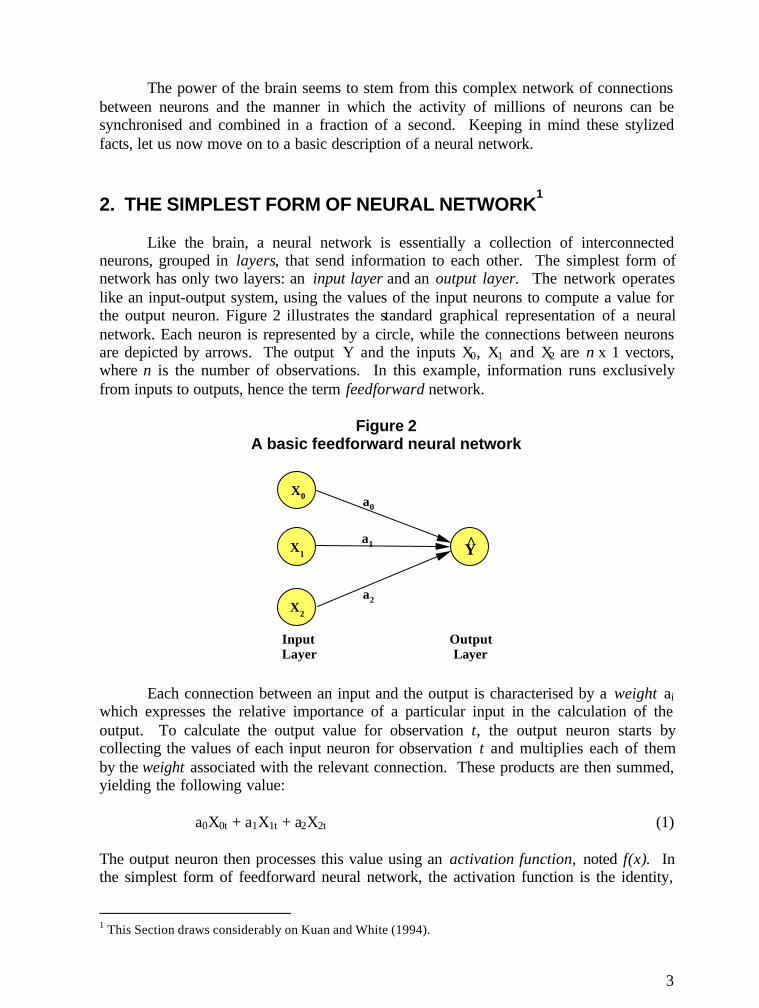
Like the brain, a neural network is essentially a collection of interconnectedneurons, grouped in layers, that send information to each other. The simplest form ofnetwork has only two layers: an input layer and an output layer. The network operateslike an input-output system, using the values of the input neurons to compute a value forthe output neuron. Figure 2 illustrates the standard graphical representation of a neuralnetwork. Each neuron is represented by a circle, while the connections between neuronsare depicted by arrows. The output Y and the inputs X0, X1 and X2 are n x 1 vectors,where n is the number of observations. In this example, information runs exclusivelyfrom inputs to outputs, hence the term feedforward network.

Figure 2A basic feedforward neural network

InputLayer

Output Layer

X0

X1

X2

a0

a1

a2

Y

Each connection between an input and the output is characterised by a weight aiwhich expresses the relative importance of a particular input in the calculation of theoutput. To calculate the output value for observation t, the output neuron starts bycollecting the values of each input neuron for observation t and multiplies each of themby the weight associated with the relevant connection. These products are then summed,yielding the following value:

a0X0t + a1X1t + a2X2t (1)

The output neuron then processes this value using an activation function, noted f(x). Inthe simplest form of feedforward neural network, the activation function is the identity,

1 This Section draws considerably on Kuan and White (1994).

4

i.e. f(x) = x. In this case, the value given in (1) would constitute the final output of thenetwork for observation t :

Yt = a0X0t + a1X1t + a2X2t (2)

Typically, one of the inputs, called the bias, is equal to 1 for all observations. Assumingthat X0 is the bias, the output of the network is given by:

Yt = a0 + a1X1t + a2X2t (3)

In general, the researcher also provides the network with the target output value(noted Yt) that the network should try to reproduce through its computations, given thevalue of the inputs. A forecasting error for each observation is then computed as thedifference between Yt and Yt. Using various iterative algorithms (the most common ofwhich is called the backpropagation algorithm), the weights of the network will bemodified until the forecasting errors across the entire sample are minimized, as measuredby the sum of squared errors or the mean absolute error. As the weights are changed witheach iteration, the network is said to be learning.

From the above discussion, it is obvious that a two-layer feedforward neuralnetwork with an identity activation function is identical to a linear regression model.The input neurons are equivalent to independent variables or regressors, while the outputneuron is the dependent variable. The various weights of the network are equivalent tothe estimated coefficients of a regression model and the bias is simply the intercept term.Note that in equations (2) and (3), the error term et is omitted as only the mathematicalexpression of the computed output value, i.e. the "fit", is being provided.

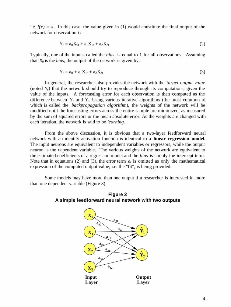
Some models may have more than one output if a researcher is interested in morethan one dependent variable (Figure 3).

Figure 3A simple feedforward neural network with two outputs

InputLayer

Output Layer

X1

X2

X3

X0a01a02

a11

a12

a21

a22

a31

a32

Y1^

Y2^

5

In this figure, aij denotes the weight that links input i to output j. Assuming again that X0

is a bias term, the network output is given by:

Y1 = a01 + a11X1 + a21X2 + a31X3

Y2 = a02 + a12X1 + a22X2 + a32X3 (4)

We obtain a system of linear equations very similar to a system of seemingly unrelatedregression equations (à la Zellner). In the presence of time-series data, we can constructa neural network equivalent to a vector autoregressive model by simply adding laggedvalues of the dependent and independent variables to the group of inputs. By introducinga link between Y1 and Y2, we would obtain a neural network equivalent to a system ofsimultaneous equations .

2.1 Nonlinear activation functions

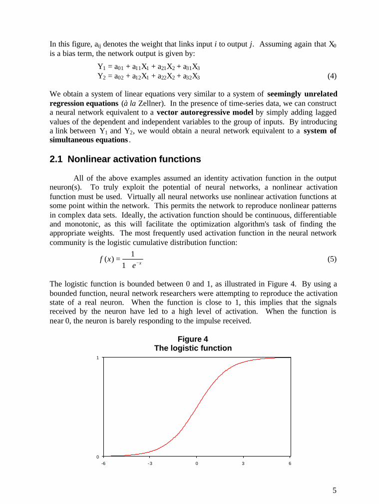
All of the above examples assumed an identity activation function in the outputneuron(s). To truly exploit the potential of neural networks, a nonlinear activationfunction must be used. Virtually all neural networks use nonlinear activation functions atsome point within the network. This permits the network to reproduce nonlinear patternsin complex data sets. Ideally, the activation function should be continuous, differentiableand monotonic, as this will facilitate the optimization algorithm's task of finding theappropriate weights. The most frequently used activation function in the neural networkcommunity is the logistic cumulative distribution function:

xexf

−+=

11

)( (5)

The logistic function is bounded between 0 and 1, as illustrated in Figure 4. By using abounded function, neural network researchers were attempting to reproduce the activationstate of a real neuron. When the function is close to 1, this implies that the signalsreceived by the neuron have led to a high level of activation. When the function isnear 0, the neuron is barely responding to the impulse received.

Figure 4The logistic function

0

1

-6 -3 0 3 6

6

If we are forecasting a variable that may take negative values, it is better to usethe hyperbolic tangent as an activation function:

)()()( xx

xx

eeeexf −

−

+−= (6)

The hyperbolic tangent function has the same profile as the logistic function, but isbounded between -1 and 1.

Returning to the simple feedforward network of Figure 2, a logistic activationfunction in the output neuron would lead to the following output for observation t :

Yt = f(a0 + a1X1t + a2X2t) = )XaXaa( t22t110e11

++−+(7)

The resulting network is the same as a binary logit probability model. If the activationfunction were a normal cumulative distribution function, we would obtain a binaryprobit model. The use of other bounded functions would yield many other networkscapable of dealing with nonlinear problems where the dependent variable is bounded.

When dealing with a dependent variable that is not bounded, we could choose anunbounded nonlinear activation function such as f(x) = x3. However, neural networkresearchers have preferred to maintain bounded activation functions, and to allow for anunbounded dependent variable by adding hidden layers to the structure of the network.

2.2 Neural networks with hidden layers

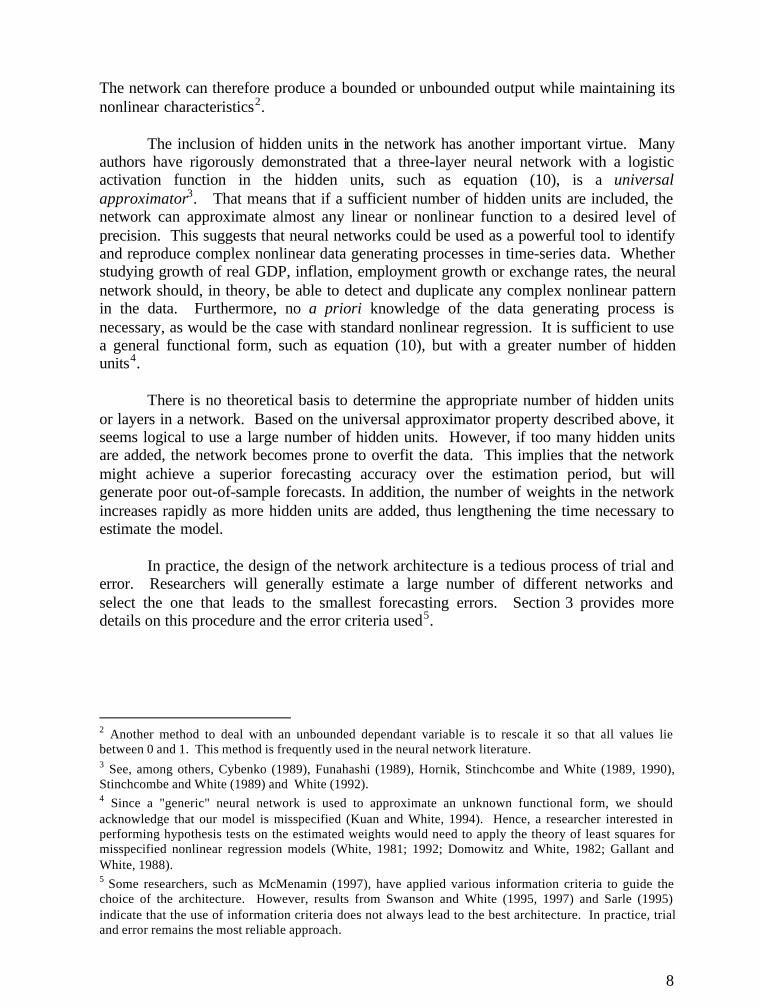
The networks described thus far had a very simple two-layer structure linkinginputs to outputs. In real world applications, the network structure is generally morecomplex. Researchers almost always design a structure that includes one or more hiddenlayers, as in Figure 5. In this figure, aij denotes the weight for the connection linkinginput i to the hidden unit j. We assume that X0 is a bias term (i.e. an intercept term) forthe hidden units while B is a bias term for the output unit.

Contrary to the input and output units, the hidden units do not represent any realconcept. They have no interpretation or meaning. They are merely an intermediate resultin the process of calculating the output value. Hence, they have no parallel ineconometrics. Hidden units behave like output units, i.e. they compute the weighted sumof the input variables and then process the result using an activation function, almostalways a logistic function. In the network illustrated in Figure 5, the result produced bythe hidden units would be:

H1 = f(a01 + a11X1 + a21X2) = )XaXaa( 22111101e11

++−+(8)

H2 = f(a02 + a12X1 + a22X2) = )XaXaa( 22211202e11

++−+(9)

7

Figure 5A feedforward neural network with one hidden layer

InputLayer

Hidden Layer

X1

X2

H 2

X0

H1

a01a02

a11

a12

a21

a22

Output Layer

b1

b2

B

b0

Y

By placing the logistic activation function in the hidden units rather than in theoutput unit, the network is no longer limited to producing estimates of bounded variables.If the dependent variable is unbounded, the output unit will generally use an identityactivation function, i.e. the output will be equal to the weighted sum of the hidden unitvalues, weighted by the bj coefficients. This will yield a continuous, nonlinear,unbounded output as expressed in equation (10):

Y = b0 + b1H1 + b2H2

Y = b0 + )XaXaa(1

22111101e1b

++−+ + )XaXaa(

222211202e1

b++−+

(10)

If the dependent variable is bounded, the output unit will generally use a logisticactivation function, thus generating a bounded output, as in equation (11):

Y = f(b0 + b1H1 + b2H2)

Y = e1

1 )Hb Hb (b- 22110 +++

++

++−

++−++−

+)2X22a1X12a02a(

2)2X21a1X11a01a(

10

e1b

e1b

b

e1

1 (11)Y =

8

The network can therefore produce a bounded or unbounded output while maintaining itsnonlinear characteristics2.

The inclusion of hidden units in the network has another important virtue. Manyauthors have rigorously demonstrated that a three-layer neural network with a logisticactivation function in the hidden units, such as equation (10), is a universalapproximator3. That means that if a sufficient number of hidden units are included, thenetwork can approximate almost any linear or nonlinear function to a desired level ofprecision. This suggests that neural networks could be used as a powerful tool to identifyand reproduce complex nonlinear data generating processes in time-series data. Whetherstudying growth of real GDP, inflation, employment growth or exchange rates, the neuralnetwork should, in theory, be able to detect and duplicate any complex nonlinear patternin the data. Furthermore, no a priori knowledge of the data generating process isnecessary, as would be the case with standard nonlinear regression. It is sufficient to usea general functional form, such as equation (10), but with a greater number of hiddenunits4.

There is no theoretical basis to determine the appropriate number of hidden unitsor layers in a network. Based on the universal approximator property described above, itseems logical to use a large number of hidden units. However, if too many hidden unitsare added, the network becomes prone to overfit the data. This implies that the networkmight achieve a superior forecasting accuracy over the estimation period, but willgenerate poor out-of-sample forecasts. In addition, the number of weights in the networkincreases rapidly as more hidden units are added, thus lengthening the time necessary toestimate the model.

In practice, the design of the network architecture is a tedious process of trial anderror. Researchers will generally estimate a large number of different networks andselect the one that leads to the smallest forecasting errors. Section 3 provides moredetails on this procedure and the error criteria used5.

2 Another method to deal with an unbounded dependant variable is to rescale it so that all values liebetween 0 and 1. This method is frequently used in the neural network literature.3 See, among others, Cybenko (1989), Funahashi (1989), Hornik, Stinchcombe and White (1989, 1990),Stinchcombe and White (1989) and White (1992).4 Since a "generic" neural network is used to approximate an unknown functional form, we shouldacknowledge that our model is misspecified (Kuan and White, 1994). Hence, a researcher interested inperforming hypothesis tests on the estimated weights would need to apply the theory of least squares formisspecified nonlinear regression models (White, 1981; 1992; Domowitz and White, 1982; Gallant andWhite, 1988).5 Some researchers, such as McMenamin (1997), have applied various information criteria to guide thechoice of the architecture. However, results from Swanson and White (1995, 1997) and Sarle (1995)indicate that the use of information criteria does not always lead to the best architecture. In practice, trialand error remains the most reliable approach.

9

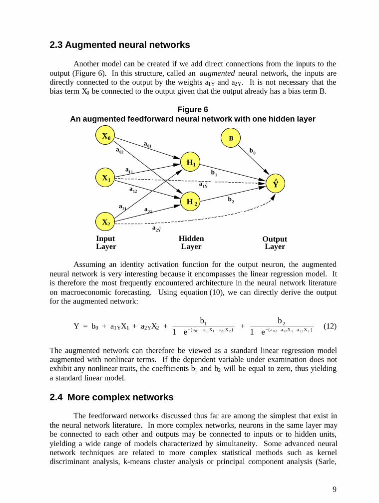
2.3 Augmented neural networks

Another model can be created if we add direct connections from the inputs to theoutput (Figure 6). In this structure, called an augmented neural network, the inputs aredirectly connected to the output by the weights a1Y and a2Y. It is not necessary that thebias term X0 be connected to the output given that the output already has a bias term B.

Figure 6An augmented feedforward neural network with one hidden layer

InputLayer

Hidden Layer

X1

X2

H 2

X0

H1

a01a02

a11

a12

a21 a22

Output Layer

b1

b2

B

b0

Ya1Y^

a2Y^

Assuming an identity activation function for the output neuron, the augmentedneural network is very interesting because it encompasses the linear regression model. Itis therefore the most frequently encountered architecture in the neural network literatureon macroeconomic forecasting. Using equation (10), we can directly derive the outputfor the augmented network:

Y = b0 + a1YX1 + a2YX2 + )XaXaa(1

22111101e1b

++−+ + )XaXaa(

222211202e1

b++−+

(12)

The augmented network can therefore be viewed as a standard linear regression modelaugmented with nonlinear terms. If the dependent variable under examination does notexhibit any nonlinear traits, the coefficients b1 and b2 will be equal to zero, thus yieldinga standard linear model.

2.4 More complex networks

The feedforward networks discussed thus far are among the simplest that exist inthe neural network literature. In more complex networks, neurons in the same layer maybe connected to each other and outputs may be connected to inputs or to hidden units,yielding a wide range of models characterized by simultaneity. Some advanced neuralnetwork techniques are related to more complex statistical methods such as kerneldiscriminant analysis, k-means cluster analysis or principal component analysis (Sarle,

10

1998). Some neural networks do not have any close parallel in statistics, such asKohonen's self-organizing maps and reinforcement learning. These advanced methodsexceed the scope of this paper and will not be addressed here. It is also uncertain whetherthese techniques could be useful for the type of forecasting performed in economics.

3. ESTIMATION OF NETWORK WEIGHTS

The network weights are estimated using a variety of iterative algorithms, themost popular being the backpropagation algorithm. Sarle (1994) argues that thesealgorithms are generally inefficient because they are very slow. Results can be obtainedmuch faster by using a standard numerical optimization algorithm such as those used innonlinear regression. Sarle (1994) concludes by stating: "Hence, for most practical dataanalysis applications, the usual neural network algorithms are not useful. You do notneed to know anything about neural network training methods such as backpropagation touse neural networks." In accordance with this view, we will not expand further on neuralnetwork training algorithms6.

Neural networkers usually divide their sample into two separate data sets. Thetraining set is used by the algorithm to estimate the network weights, while the test set isused to evaluate the forecasting accuracy of the network. Since the test set is not usedduring the estimation of the network weights, the forecasts made from the test set amountto an ex post out-of-sample forecast. The neural networker aims at minimizing theforecasting error in the training set using a criterion such as the mean squared error(MSE).

3.1 Early stopping

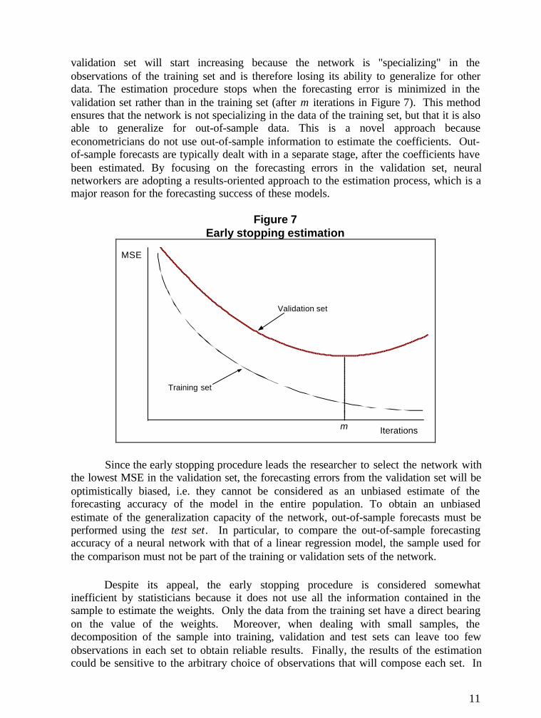
Experience has shown that neural networks are prone to overfit the data in thetraining set, thus yielding poor out-of-sample forecasts. To minimize this problem,several procedures have been developed. One of the most frequently used procedures iscalled early stopping7, which involves the division of the data set into three parts: atraining set, a test set and a validation set. As discussed above, the training set is used bythe algorithm to estimate the network weights, while the test set is set aside for out-of-sample forecasting. The validation set is a portion of the data that is not used during thetraining (i.e. the algorithm never "sees" the validation set), but which serves as anindicator of the out-of-sample forecasting accuracy of the network. After each iterationin the estimation process, an out-of-sample forecast is generated using the observations inthe validation set and the MSE is calculated. Figure 7 shows the typical evolution of theMSE in the training and validation sets throughout the estimation process. As the numberof iterations increases, the MSE in both the training and validation sets will generallydecline. Experience suggests that after a certain number of iterations, the MSE in the

6 The interested reader is referred to Gibb (1996) for a discussion on training algorithms.7 Sarle (1998) discusses other commonly used methods to minimize the overfitting problem, such as"weight decay" and adding "noise" to the inputs.

11

validation set will start increasing because the network is "specializing" in theobservations of the training set and is therefore losing its ability to generalize for otherdata. The estimation procedure stops when the forecasting error is minimized in thevalidation set rather than in the training set (after m iterations in Figure 7). This methodensures that the network is not specializing in the data of the training set, but that it is alsoable to generalize for out-of-sample data. This is a novel approach becauseeconometricians do not use out-of-sample information to estimate the coefficients. Out-of-sample forecasts are typically dealt with in a separate stage, after the coefficients havebeen estimated. By focusing on the forecasting errors in the validation set, neuralnetworkers are adopting a results-oriented approach to the estimation process, which is amajor reason for the forecasting success of these models.

Figure 7Early stopping estimation

Iterations

MSE

Training set

Validation set

m

Since the early stopping procedure leads the researcher to select the network withthe lowest MSE in the validation set, the forecasting errors from the validation set will beoptimistically biased, i.e. they cannot be considered as an unbiased estimate of theforecasting accuracy of the model in the entire population. To obtain an unbiasedestimate of the generalization capacity of the network, out-of-sample forecasts must beperformed using the test set. In particular, to compare the out-of-sample forecastingaccuracy of a neural network with that of a linear regression model, the sample used forthe comparison must not be part of the training or validation sets of the network.

Despite its appeal, the early stopping procedure is considered somewhatinefficient by statisticians because it does not use all the information contained in thesample to estimate the weights. Only the data from the training set have a direct bearingon the value of the weights. Moreover, when dealing with small samples, thedecomposition of the sample into training, validation and test sets can leave too fewobservations in each set to obtain reliable results. Finally, the results of the estimationcould be sensitive to the arbitrary choice of observations that will compose each set. In

12

spite of these shortcomings, the early stopping procedure is frequently used in theliterature and has enabled researchers to develop accurate networks.

3.2 Designing the model

When an econometrician is building a linear regression model for forecastingpurposes, a significant part of the work consists in identifying the explanatory variablesand the number of lags that will allow the most accurate forecasts. This will generallyrequire many hours of experimentation with alternative specifications. Fortunately, theestimation of each alternative specification is instantaneous and the out-of-sampleforecasts can be rapidly generated and assessed. Once the researcher has found thespecification that minimizes the forecasting errors, a substantial portion of the work iscompleted and the researcher can then focus his/her efforts on diagnostic tests.

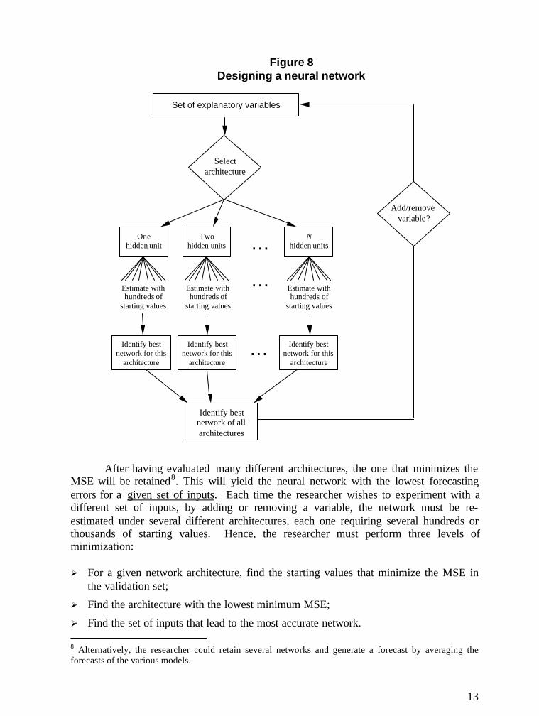
When constructing a neural network, the overall task is much longer. The neuralnetworker must not only choose a set of inputs, but must also identify the networkarchitecture that leads to the best forecasts. Changes to the architecture canfundamentally alter the forecasts produced by the network, even when no changes aremade to the inputs, outputs or sample size. To find the best architecture, the neuralnetworker must proceed by trial and error. This process is summarized in Figure 8.

As with any nonlinear estimation technique, one can never be sure that the globalminimum has been attained. In practice, this implies that the results of the estimationprocedure are sensitive to the initial values of the weights. Thus, for a given set of inputsand a given network architecture, the early stopping procedure described above must berepeated hundreds or thousands of times using different starting values for the weights.The estimated weights that lead to the lowest MSE in the validation set will be consideredas the best possible outcome for that specific network architecture and for the specific setof inputs that was used in the network.

To assess the performance of other architectures, the researcher must modify thearchitecture of the network by changing the number of hidden units or by adding orremoving certain network connections. The whole early stopping procedure must againbe repeated hundreds of times in the new architecture, by varying the starting values, inthe hope of finding the global minimum. The two architectures may then be evaluated bycomparing the minimum of the MSE attained in each architecture.

13

Figure 8Designing a neural network

…

Set of explanatory variables

Selectarchitecture

Onehidden unit

Twohidden units … N

hidden units

Estimate withhundreds of

starting values

Identify bestnetwork for this

architecture

…

Identify bestnetwork of allarchitectures

Add/remove variable?

Estimate withhundreds of

starting values

Estimate withhundreds of

starting values

Identify bestnetwork for this

architecture

Identify bestnetwork for this

architecture

After having evaluated many different architectures, the one that minimizes theMSE will be retained8. This will yield the neural network with the lowest forecastingerrors for a given set of inputs. Each time the researcher wishes to experiment with adifferent set of inputs, by adding or removing a variable, the network must be re-estimated under several different architectures, each one requiring several hundreds orthousands of starting values. Hence, the researcher must perform three levels ofminimization:

Ø For a given network architecture, find the starting values that minimize the MSE inthe validation set;

Ø Find the architecture with the lowest minimum MSE;

Ø Find the set of inputs that lead to the most accurate network. 8 Alternatively, the researcher could retain several networks and generate a forecast by averaging theforecasts of the various models.

14

When designing a linear regression model, only the last stage of minimizationneeds to be done, i.e. the selection of the most relevant set of explanatory variables.Thus, it is clear that the design of a neural network is much more time consuming thanthe design of a linear model. Fortunately, this process can be somewhat shortened with alittle programming. As will be explained later, the use of a linear regression model toassist in the selection of the inputs can also greatly reduce the length of this process.

4. AN APPLICATION TO REAL GDP FORECASTING

An empirical example is perhaps the best way to illustrate the differences betweena neural network and a linear regression model. A neural network has therefore beenconstructed to forecast quarterly growth of Canada's real GDP. This model is comparedto a linear regression model developed in the Department of Finance by Lamy (1999). Tofacilitate the comparison, the neural network uses exactly the same explanatory variablesand the same sample period as the linear regression model. Any differences in the resultscan therefore be attributed solely to the estimation procedure.

4.1 The linear regression model

Lamy (1999) has developed an accurate model for one-quarter ahead forecasts ofquarterly growth of Canada's real GDP. The model has performed very well, both in-sample and out-of-sample. Over the period from 1978Q1 to 1998Q2, his model explains82 per cent of the variance of real GDP growth. The estimated coefficients are also verystable when the model is estimated over different sample periods. In addition, the modelis quite parsimonious, as it contains only the following six explanatory variables (withtheir abbreviation in parenthesis):

Ø The quarterly growth rate of Finance Canada's index of leading indicators ofeconomic activity (one-quarter lag) (Lt-1)

Ø Employment growth (contemporaneous) (Et)Ø Employment growth (one-quarter lag) (Et-1)Ø The Conference Board's index of consumer confidence (contemporaneous) (Ct)Ø The first difference of the real long term interest rate (nine-quarter lag) (Rt-9)Ø The first difference of the federal government budgetary balance as a share of GDP

(three-quarter lag) (Ft-3)

Four dummy variables were added to control for four quarters considered asoutliers9. For the purposes of the present illustration and in order to leave some data forout-of-sample forecasts, the linear regression model was estimated using data from1978Q1 to 1993Q2 (62 observations). The estimation results are given in equation (13):

GDPt = -1.695 + 0.075·Lt-1 + 0.304·Et + 0.251·Et-1 + 0.019·Ct - 0.175·Rt-9

- 0.320·Ft-3 - 1.155·D1 + 1.168·D2 - 0.906·D3 - 0.843·D4 + et (13) 9 The four quarters in question are 1980Q3, 1981Q1, 1986Q4 and 1991Q3.

15

where D1, D2, D3 and D4 are the dummy variables and et is the residual term. Allcoefficients are significantly different from zero at a confidence level of 95 per cent.

4.2 The neural network equivalent

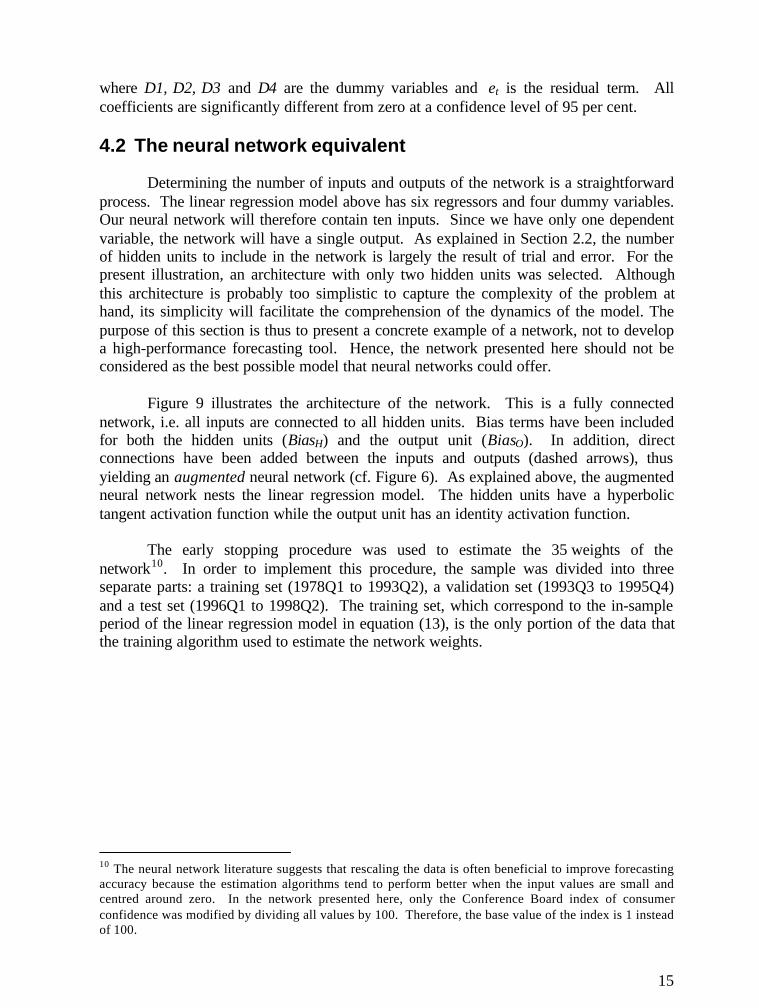
Determining the number of inputs and outputs of the network is a straightforwardprocess. The linear regression model above has six regressors and four dummy variables.Our neural network will therefore contain ten inputs. Since we have only one dependentvariable, the network will have a single output. As explained in Section 2.2, the numberof hidden units to include in the network is largely the result of trial and error. For thepresent illustration, an architecture with only two hidden units was selected. Althoughthis architecture is probably too simplistic to capture the complexity of the problem athand, its simplicity will facilitate the comprehension of the dynamics of the model. Thepurpose of this section is thus to present a concrete example of a network, not to developa high-performance forecasting tool. Hence, the network presented here should not beconsidered as the best possible model that neural networks could offer.

Figure 9 illustrates the architecture of the network. This is a fully connectednetwork, i.e. all inputs are connected to all hidden units. Bias terms have been includedfor both the hidden units (BiasH) and the output unit (BiasO). In addition, directconnections have been added between the inputs and outputs (dashed arrows), thusyielding an augmented neural network (cf. Figure 6). As explained above, the augmentedneural network nests the linear regression model. The hidden units have a hyperbolictangent activation function while the output unit has an identity activation function.

The early stopping procedure was used to estimate the 35 weights of thenetwork10. In order to implement this procedure, the sample was divided into threeseparate parts: a training set (1978Q1 to 1993Q2), a validation set (1993Q3 to 1995Q4)and a test set (1996Q1 to 1998Q2). The training set, which correspond to the in-sampleperiod of the linear regression model in equation (13), is the only portion of the data thatthe training algorithm used to estimate the network weights.

10 The neural network literature suggests that rescaling the data is often beneficial to improve forecastingaccuracy because the estimation algorithms tend to perform better when the input values are small andcentred around zero. In the network presented here, only the Conference Board index of consumerconfidence was modified by dividing all values by 100. Therefore, the base value of the index is 1 insteadof 100.

16

Figure 9An augmented neural network to forecast real GDP growth

InputLayer

Hidden Layer

Output Layer

Lt-1

Et

Et-1

Ct

Rt-9

Ft-3

D1

D2

D3

D4

GDPt

H1

H2

BiasH

BiasO

17

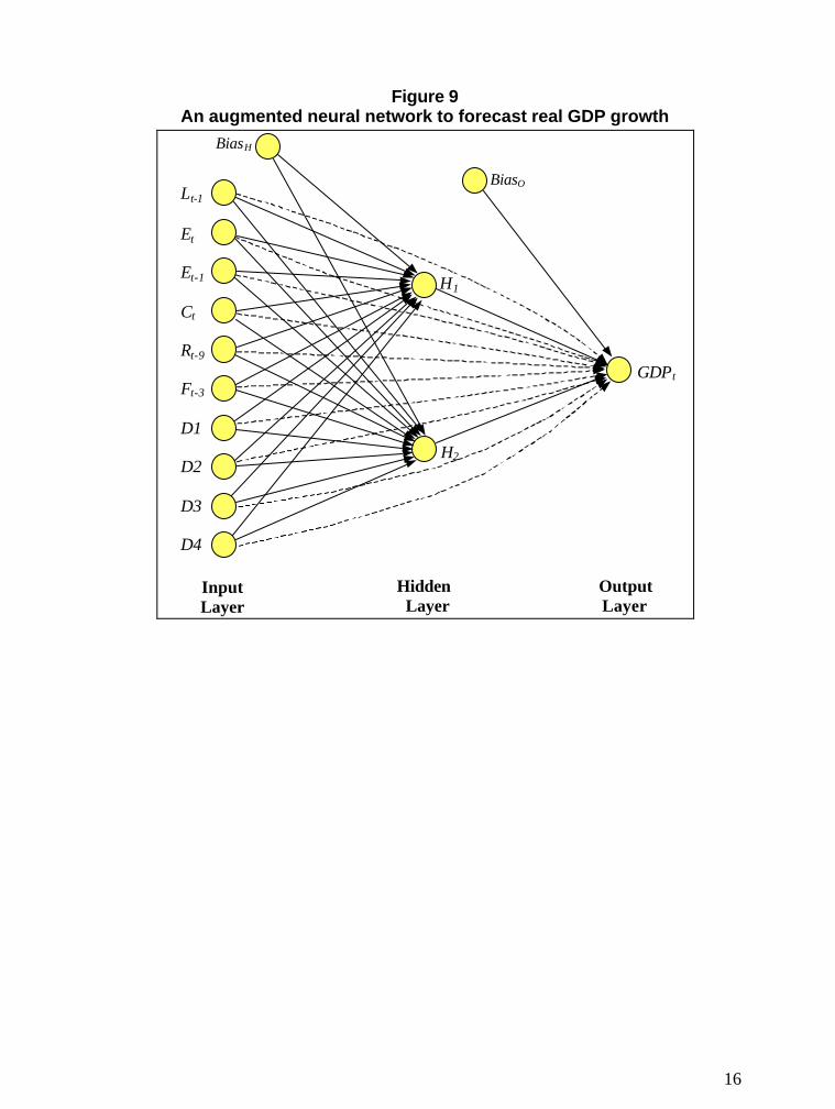
Figure 10 illustrates the evolution of the mean absolute error (MAE)11 in thetraining and validation sets throughout the iteration process. The MAE in the validationset reaches a minimum after 819 iterations, while the MAE in the training set continues todecline continuously. To reduce the risk of overfitting the network, the procedure wastherefore stopped after 819 iterations, with a MAE of 0.118 in the validation set.

Figure 10Results of the early stopping estimation procedure

0

0.1

0.2

0.3

0.4

0.5

0.6

0.7

0.8

1 200 400 600 800 1000 1200 1400 1600

MAE

Iterations

Validation set

Training set

Minimum

11 The software used to estimate the network weights (MATLAB with the Netlab toolbox) was programmedto provide the mean absolute forecasting error, rather than the mean squared error as discussed in Section 3.This does not have a significant effect on the results. The Netlab toolbox can be downloaded free of chargefrom http://www.ncrg.aston.ac.uk/netlab/index.html.

18

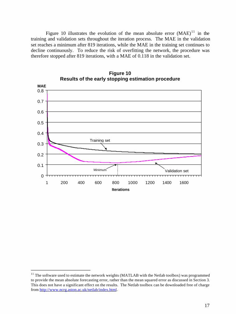
In Figure 11, the estimated weights are presented for various sections of thenetwork. The connections from the inputs and BiasH to the hidden unit H1 are presentedin Panel A. Panel B presents a similar diagram for the connections between the inputsand H2. Panel C displays the estimated weights between the hidden units and the outputunit and Panel D illustrated the direct connections from the inputs to the output.

Figure 11Estimated weights

Panel A

Lt-1

Et

Et-1

Ct

Rt-9

Ft-3

D1

D2

D3

D4

H1

BiasH

-0.058

0.292

-0.401

-0.207

0.550

0.754

0.294

-1.038

0.487

-0.290

-0.209

Panel B

Lt-1

Et

Et-1

Ct

Rt-9

Ft-3

D1

D2

D3

D4

H2

BiasH

-0.327

0.229

-0.731

-0.732

-0.269

0.666

0.085

0.325

-0.317

-0.229

-0.072

Panel C

GDP t

H1

H2

BiasO

1.450

0.604

-0.081

Panel D

Lt-1

Et

Et-1

Ct

Rt-9

Ft-3

D1

D2

D3

D4

GDPt

0.084

0.335

0.751

0.339

-1.067

-0.649

0.048

0.210

-0.256

-0.550

19

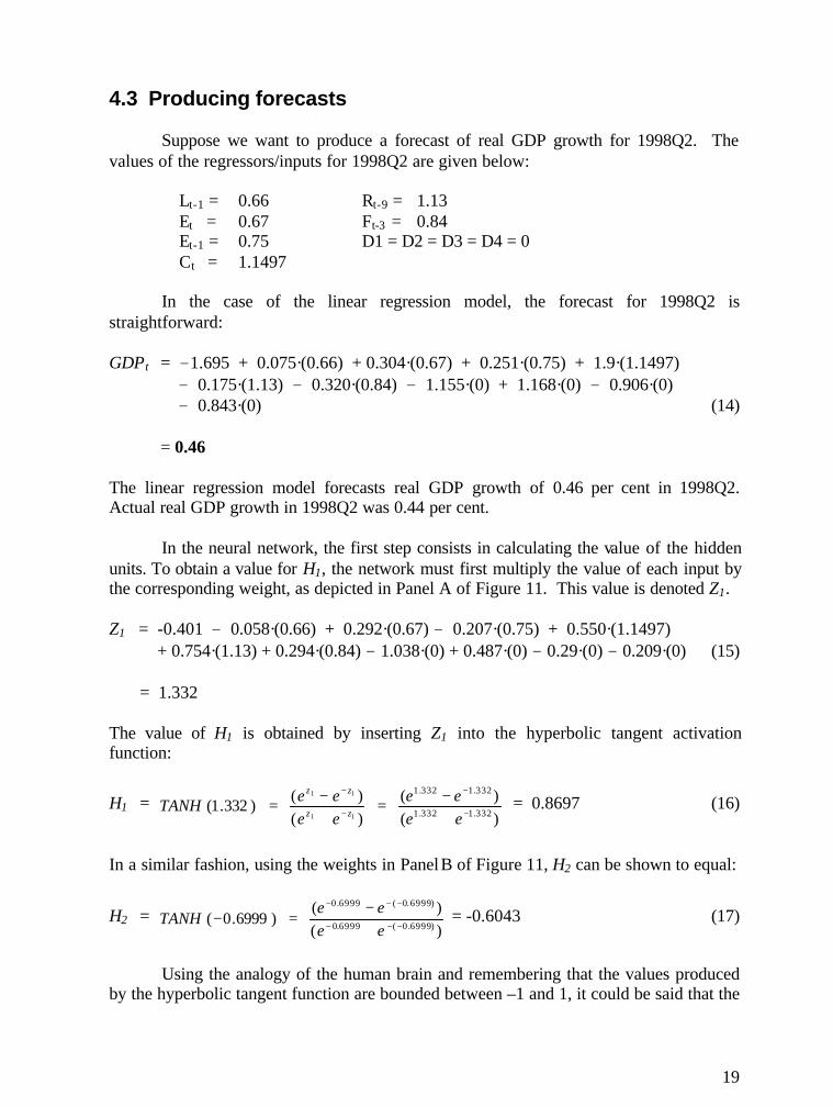
4.3 Producing forecasts

Suppose we want to produce a forecast of real GDP growth for 1998Q2. Thevalues of the regressors/inputs for 1998Q2 are given below:

Lt-1 = 0.66 Rt-9 = 1.13Et = 0.67 Ft-3 = 0.84Et-1 = 0.75 D1 = D2 = D3 = D4 = 0Ct = 1.1497

In the case of the linear regression model, the forecast for 1998Q2 isstraightforward:

GDPt = -1.695 + 0.075·(0.66) + 0.304·(0.67) + 0.251·(0.75) + 1.9·(1.1497) - 0.175·(1.13) - 0.320·(0.84) - 1.155·(0) + 1.168·(0) - 0.906·(0) - 0.843·(0) (14)

= 0.46

The linear regression model forecasts real GDP growth of 0.46 per cent in 1998Q2.Actual real GDP growth in 1998Q2 was 0.44 per cent.

In the neural network, the first step consists in calculating the value of the hiddenunits. To obtain a value for H1, the network must first multiply the value of each input bythe corresponding weight, as depicted in Panel A of Figure 11. This value is denoted Z1.

Z1 = -0.401 - 0.058·(0.66) + 0.292·(0.67) – 0.207·(0.75) + 0.550·(1.1497) + 0.754·(1.13) + 0.294·(0.84) – 1.038·(0) + 0.487·(0) - 0.29·(0) - 0.209·(0) (15)

= 1.332

The value of H1 is obtained by inserting Z1 into the hyperbolic tangent activationfunction:

H1 = )()(

)()()332.1( 332.1332.1

332.1332.1

11

11

−

−

−

−

+−=

+−=

eeee

eeeeTANH zz

zz

= 0.8697 (16)

In a similar fashion, using the weights in Panel B of Figure 11, H2 can be shown to equal:

H2 = )()(

)6999.0( )6999.0(6999.0

)6999.0(6999.0

−−−

−−−

+−

=−eeee

TANH = -0.6043 (17)

Using the analogy of the human brain and remembering that the values producedby the hyperbolic tangent function are bounded between –1 and 1, it could be said that the

20

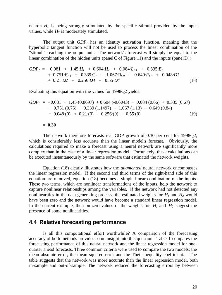
neuron H1 is being strongly stimulated by the specific stimuli provided by the inputvalues, while H2 is moderately stimulated.

The output unit GDPt has an identity activation function, meaning that thehyperbolic tangent function will not be used to process the linear combination of the"stimuli" reaching the output unit. The network's forecast will simply be equal to thelinear combination of the hidden units (panel C of Figure 11) and the inputs (panel D):

GDPt = -0.081 + 1.45·H1 + 0.604·H2 + 0.084·Lt-1 + 0.335·Et

+ 0.751·Et-1 + 0.339·Ct - 1.067·Rt-9 - 0.649·Ft-3 + 0.048·D1 + 0.21·D2 - 0.256·D3 - 0.55·D4 (18)

Evaluating this equation with the values for 1998Q2 yields:

GDPt = -0.081 + 1.45·(0.8697) + 0.604·(-0.6043) + 0.084·(0.66) + 0.335·(0.67) + 0.751·(0.75) + 0.339·(1.1497) - 1.067·(1.13) - 0.649·(0.84) + 0.048·(0) + 0.21·(0) - 0.256·(0) - 0.55·(0) (19)

= 0.30

The network therefore forecasts real GDP growth of 0.30 per cent for 1998Q2,which is considerably less accurate than the linear model's forecast. Obviously, thecalculations required to make a forecast using a neural network are significantly morecomplex than in the case of a linear regression model. Fortunately, these calculations canbe executed instantaneously by the same software that estimated the network weights.

Equation (18) clearly illustrates how the augmented neural network encompassesthe linear regression model. If the second and third terms of the right-hand side of thisequation are removed, equation (18) becomes a simple linear combination of the inputs.These two terms, which are nonlinear transformations of the inputs, help the network tocapture nonlinear relationships among the variables. If the network had not detected anynonlinearities in the data generating process, the estimated weights for H1 and H2 wouldhave been zero and the network would have become a standard linear regression model.In the current example, the non-zero values of the weights for H1 and H2 suggest thepresence of some nonlinearities.

4.4 Relative forecasting performance

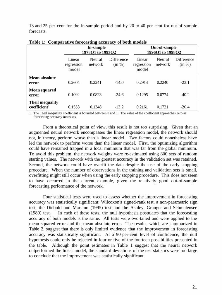
Is all this computational effort worthwhile? A comparison of the forecastingaccuracy of both methods provides some insight into this question. Table 1 compares theforecasting performance of this neural network and the linear regression model for one-quarter ahead forecasts. Three common criteria were used to compare the two models: themean absolute error, the mean squared error and the Theil inequality coefficient. Thetable suggests that the network was more accurate than the linear regression model, bothin-sample and out-of-sample. The network reduced the forecasting errors by between

21

13 and 25 per cent for the in-sample period and by 20 to 40 per cent for out-of-sampleforecasts.

Table 1: Comparative forecasting accuracy of both modelsIn-sample

1978Q1 to 1993Q2 Out-of-sample

1996Q1 to 1998Q2

Linearregression

model

Neuralnetwork

Difference(in %)

Linearregression

model

Neuralnetwork

Difference(in %)

Mean absoluteerror 0.2604 0.2241 -14.0 0.2914 0.2240 -23.1

Mean squarederror 0.1092 0.0823 -24.6 0.1295 0.0774 -40.2

Theil inequalitycoefficient1 0.1553 0.1348 -13.2 0.2161 0.1721 -20.41. The Theil inequality coefficient is bounded between 0 and 1. The value of the coefficient approaches zero as

forecasting accuracy increases.

From a theoretical point of view, this result is not too surprising. Given that anaugmented neural network encompasses the linear regression model, the network shouldnot, in theory, perform worse than a linear model. Two factors could nonetheless haveled the network to perform worse than the linear model. First, the optimizing algorithmcould have remained trapped in a local minimum that was far from the global minimum.To avoid this problem, the network weights were re-estimated using 800 sets of randomstarting values. The network with the greatest accuracy in the validation set was retained.Second, the network could have overfit the data despite the use of the early stoppingprocedure. When the number of observations in the training and validation sets is small,overfitting might still occur when using the early stopping procedure. This does not seemto have occurred in the current example, given the relatively good out-of-sampleforecasting performance of the network.

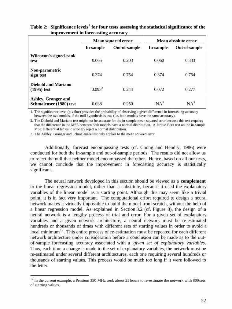
Four statistical tests were used to assess whether the improvement in forecastingaccuracy was statistically significant: Wilcoxon's signed-rank test, a non-parametric signtest, the Diebold and Mariano (1995) test and the Ashley, Granger and Schmalensee(1980) test. In each of these tests, the null hypothesis postulates that the forecastingaccuracy of both models is the same. All tests were two-tailed and were applied to themean squared error and the mean absolute error. The results, which are summarized inTable 2, suggest that there is only limited evidence that the improvement in forecastingaccuracy was statistically significant. At a 90-per-cent level of confidence, the nullhypothesis could only be rejected in four or five of the fourteen possibilities presented inthe table. Although the point estimates in Table 1 suggest that the neural networkoutperformed the linear model, the standard deviations of the test statistics were too largeto conclude that the improvement was statistically significant.

22

Table 2: Significance levels1 for four tests assessing the statistical significance of theimprovement in forecasting accuracy

Mean squared error Mean absolute error In-sample Out-of-sample In-sample Out-of-sample

Wilcoxon's signed-ranktest 0.065 0.203 0.060 0.333

Non-parametricsign test 0.374 0.754 0.374 0.754

Diebold and Mariano(1995) test 0.0952 0.244 0.072 0.277

Ashley, Granger andSchmalensee (1980) test 0.038 0.250 NA3 NA3

1. The significance level (p-value) provides the probability of observing a given difference in forecasting accuracybetween the two models, if the null hypothesis is true (i.e. both models have the same accuracy).

2. The Diebold and Mariano test might not be accurate for the in-sample mean squared error because this test requiresthat the difference in the MSE between both models have a normal distribution. A Jarque-Bera test on the in-sampleMSE differential led us to strongly reject a normal distribution.

3. The Ashley, Granger and Schmalensee test only applies to the mean squared error.

Additionally, forecast encompassing tests (cf. Chong and Hendry, 1986) wereconducted for both the in-sample and out-of-sample periods. The results did not allow usto reject the null that neither model encompassed the other. Hence, based on all our tests,we cannot conclude that the improvement in forecasting accuracy is statisticallysignificant.

The neural network developed in this section should be viewed as a complementto the linear regression model, rather than a substitute, because it used the explanatoryvariables of the linear model as a starting point. Although this may seem like a trivialpoint, it is in fact very important. The computational effort required to design a neuralnetwork makes it virtually impossible to build the model from scratch, without the help ofa linear regression model. As explained in Section 3.2 (cf. Figure 8), the design of aneural network is a lengthy process of trial and error. For a given set of explanatoryvariables and a given network architecture, a neural network must be re-estimatedhundreds or thousands of times with different sets of starting values in order to avoid alocal minimum12. This entire process of re-estimation must be repeated for each differentnetwork architecture under consideration before a conclusion can be made as to the out-of-sample forecasting accuracy associated with a given set of explanatory variables.Thus, each time a change is made to the set of explanatory variables, the network must bere-estimated under several different architectures, each one requiring several hundreds orthousands of starting values. This process would be much too long if it were followed tothe letter.

12 In the current example, a Pentium 350 MHz took about 25 hours to re-estimate the network with 800 setsof starting values.

23

It is far more efficient to start by using a linear regression model to experimentwith different sets of explanatory variables. Once a satisfactory set of variables has beenidentified, the researcher can proceed to evaluate different architectures. Thus, one of thethree levels of minimization identified in Section 3.2 can be greatly shortened using alinear regression model. The linear model is thus an essential tool to facilitate theimplementation of a neural network.

5. OTHER EXAMPLES OF NEURAL NETWORK APPLICATIONS

Obviously, one empirical example cannot serve as a basis to assess theeffectiveness of neural networks. The empirical literature on the subject providesadditional information in this respect. This section presents only a sample of the workthat has been done. Much of the research performed in the fields of economics andfinance has focused on forecasting the behaviour of various financial instruments, such asexchange rates or the prices of stocks, options and commodities. In this section, we willemphasize studies that forecast macroeconomic variables of interest to economists.

5.1 Encouraging results

The literature on neural networks contains numerous articles that proclaim theusefulness of these models for various forecasting exercices. However, as stressed byChatfield (1993), many of these papers are unreliable because they lack methodologicalrigour. One frequently encountered deficiency occurs when researchers use theobservations of their test set to guide the training process. Tal and Nazareth (1995) andAndersson and Falksund (1994) seem to have fallen into this trap. As explained inSection 3.2, the resulting forecasting errors are biased in favour of the neural network.Other authors provide their neural network with many more explanatory variables thanthe competing models (e.g. Bramson and Hoptroff, 1990), thus making the comparisonsomewhat unfair. Some authors do not even attempt to compare the accuracy of theirnetworks with that of competing models. The authors simply calculate the averageforecasting errors of their networks and conclude that the errors are “small” (e.g. Aiken,1999 and Aiken and Bsat, 1999).

This kind of result cannot be used to judge the relative merits of neural networks.Thus, in the following discussion, we will only mention the articles that seem to haveapplied a more rigorous methodology. As will be shown, the literature suggests thatneural networks perform well for forecasting economic output and various financialvariables.

Hill et al. (1994) surveyed the literature comparing the forecasting performance ofneural networks and statistical models. In the studies surveyed, neural networksperformed as well as or better than standard statistical techniques for the forecasting ofmacroeconomic variables, measured in terms of the mean absolute percentage error. Intime-series applications, results from some papers suggested that neural networks weremore accurate in the later periods of the forecast horizon. They also seemed to perform

24

better for higher frequency data (i.e. with monthly and quarterly data), leading the authorsto speculate that higher frequency data contained more nonlinearities. However, theauthors concluded that the literature on the subject was still inconclusive.

This relatively positive outlook for neural networks is confirmed by three studiesattempting to forecast economic output. Tkacz (1999) compared the accuracy of linearmodels and neural networks in forecasting Canada's real GDP growth using a series offinancial indicators. At the 1-quarter and 4-quarter horizons, neural networks producedmore accurate out-of-sample forecasts than the linear models. Using various tests, theimprovement in forecasting accuracy obtained by the networks was generally found to bestatistically significant. The author concluded that the networks may have been capturingsome nonlinearities in the relationship between real GDP growth and financial indicators.Similarly, Fu (1998) found that neural networks outperformed linear regression modelsfor out-of-sample forecasts of US real GDP growth. The neural networks were able toreduce the out-of-sample sum of squared residuals by between 10 and 20 per cent.Moody, Levin and Rehfuss (1993) obtained analogous results when forecasting thegrowth rate of the U.S. Index of Industrial Production. For all forecast horizonsconsidered (which ranged from 1 to 12 months ahead), their two neural networks werefound to be more accurate than a univariate autoregressive model and a multivariatelinear regression model.

In the field of financial markets, several studies have reported favourable resultsregarding neural networks. We will only discuss two studies that focus on variables ofinterest to macroeconomists. Verkooijen (1996) compared the accuracy of variousmodels in forecasting the monthly US dollar–Deutsche Mark exchange rate at horizonsvarying between 1 and 36 months ahead. For out-of-sample forecasts, the neural networkmodels were found to be slightly more accurate than linear regression models and randomwalk forecasts, particularly at longer forecast horizons. The relative performance of thenetworks was even better when forecasting the direction of change of the exchange rate.In another study, Refenes, Zapranis and Francis (1994) compared the accuracy of afeedforward neural network and a multivariate linear regression model in forecastingstock performance within the framework of the arbitrage pricing theory. Their resultsshowed that the neural network was more precise for both in-sample and out-of-sampleforecasting.

Donaldson and Kamstra (1996) produced perhaps the only study examining theadvantages of using neural networks to combine the forecasts of various models. Theindividual forecasts in their combining exercise were forecasts of the volatility of dailyreturns of four major stock market indices, as produced by a moving-average variancemodel (MAV) and a GARCH(1,1) model. When these individual forecasts werecombined with neural networks, the resulting forecast generally had a lower out-of-sample mean squared error than when they were combined with linear techniques, suchas the simple average of individual forecasts or a weighted sum of individual forecasts.Furthermore, encompassing tests revealed that the neural network pooled forecastencompassed several of the other pooled forecasts, but it was the only model that was

25

never encompassed by any other. Thus, they concluded that neural network combiningproduced better forecasts than the more traditional combining methods.

5.2 Less promising results

Church and Curram (1996) seems to be the only reliable study that has not foundneural networks to be more accurate than linear models for macroeconomic forecasting.These authors compared the accuracy of neural networks with some linear models inforecasting aggregate consumption in the U.K. in the late 1980s. The linear models weretaken from the literature that has sought to explain the significant decline in the growthrate of consumer spending in the late 1980s. Using the same explanatory variables as inthe linear models, the networks produced forecasts that were equivalent to but no betterthan the linear forecasts. They conclude that, regardless of which type of model isestimated, the choice of explanatory variables is the main determinant of forecastingaccuracy.

Although three other studies have concluded that neural networks are no betterthan linear models, these papers contain methodological deficiencies that make theirresults less reliable. These three studies will be discussed below, since they have receivedsome attention in the economic literature on neural networks.

To our knowledge, Stock and Watson (1998) is the largest forecastingcompetition for macroeconomic time series that includes neural networks. A total of49 univariate forecasting methods – including 15 feedforward neural networks – andvarious forecast pooling procedures were used to forecast 215 U.S. monthlymacroeconomic time series at three forecasting horizons. The various pooling proceduresprovided the most accurate out-of-sample forecasts, suggesting that neural networks mayhelp improve forecasting accuracy when combined with other forecasts13. However,when comparing the out-of-sample forecasting accuracy of individual models, the neuralnetworks performed poorly relative to a "naïve" AR(4) forecast and relative to most othermethods in the competition. The networks were also worse than the only other nonlinearmethod included in the competition, the logistic smooth transition autoregression model.Unfortunately, it does not appear that the authors applied the early stopping procedure orany other method to minimize the overfitting problem. This would explain the poor out-of-sample forecasting performance of their networks. In addition, it seems that arelatively small number of parameter vectors were used as initial values for the Gauss-Newton minimizing algorithm, thus reducing the likelihood of finding a solution close tothe global minimum. These two factors, combined with the fact that the paper onlyexamined univariate models, limit the scope of their results.

In another forecasting competition, Swanson and White (1997) compared variousmethodologies for forecasting nine U.S. macroeconomic variables. The methods studiedincluded autoregressive models, vector autoregressive systems, feedforward neural

13 The literature contains very little research on the merits of combining neural network forecasts with thoseof other models. Further research in this area would be very useful.

26

networks, professional "consensus" forecasts and a "no change" rule. A similarmethodology was used in Swanson and White (1995) to compare various models for out-of-sample forecasting of spot interest rates. In both papers, the neural networks posted arather ordinary performance. However, two factors tend to reduce the scope of theseresults. First, as in the case of Stock and Watson (1998), it seems that the authors did notapply any procedure to minimize the overfitting problem. Furthermore, the architecturesfor all the networks in Swanson and White (1995 and 1997) were selected using theSchwarz Information Criterion (SIC). After discussing the results in their 1997 paper, theauthors acknowledged that this criterion "cannot reliably be used as a shortcut toidentifying models that will perform optimally out of sample." A little further, theyconcluded that "in-sample SIC does not appear to offer a convenient shortcut to true out-of-sample performance measures for selecting models, or for configuring ANN [ArtificialNeural Network] models when forecasting macroeconomic variables." The wording ofthe conclusion in the 1995 paper is almost identical to the above quotes. Hence, theirconclusions suggest that the framework of their papers and the use of the SIC did not dojustice to the true potential of the neural network methodology.

As it can be seen from the above discussion, the empirical literature on neuralnetworks does not offer a unanimous verdict, as empirical evidence on macroeconomicforecasting remains sparse. This problem is compounded by the fact that many studiesseem to have methodological deficiencies. As suggested by Chatfield (1993), a greatereffort must be made to establish fair comparisons between both approaches before anyfirm conclusions can be reached.

Overall, there seem to be more studies that conclude in favour of neural networksthan against them. However, since the literature is not entirely conclusive, it may bepreferable to examine the relative advantages and disadvantages of neural networks froma more theoretical point of view. This may help us isolate the areas where theirapplication may be potentially fruitful.

6. RELATIVE STRENGTHS AND WEAKNESSES OF NEURALNETWORKS VERSUS OTHER STATISTICAL TECHNIQUES

Despite progress made in nonlinear regression theory, the vast majority ofapplications in econometrics continue to assume a linear relationship between thedependent variable and the regressors. The simplicity of the linear model and thepossibility of linearizing certain nonlinear relationships make the linear regression modela very attractive and powerful tool. The largest part of our discussion will therefore focuson comparing neural networks to linear regression models. Table 3 summarizes therelative strengths and weaknesses of neural networks that will be discussed in thefollowing sections.

27

Table 3: Relative strengths and weaknesses of neural networksStrengths

Can successfully model nonlinear relationshipsDo not require a priori information on the functional form of a relationshipThe same architecture is very flexible

WeaknessesIt is difficult to interpret the estimated network weights ("black box" problem)Unlikely to find the global minimumUsually require large samplesThe construction of the network architecture can be time consuming.

6.1 Relative strengths of neural networks

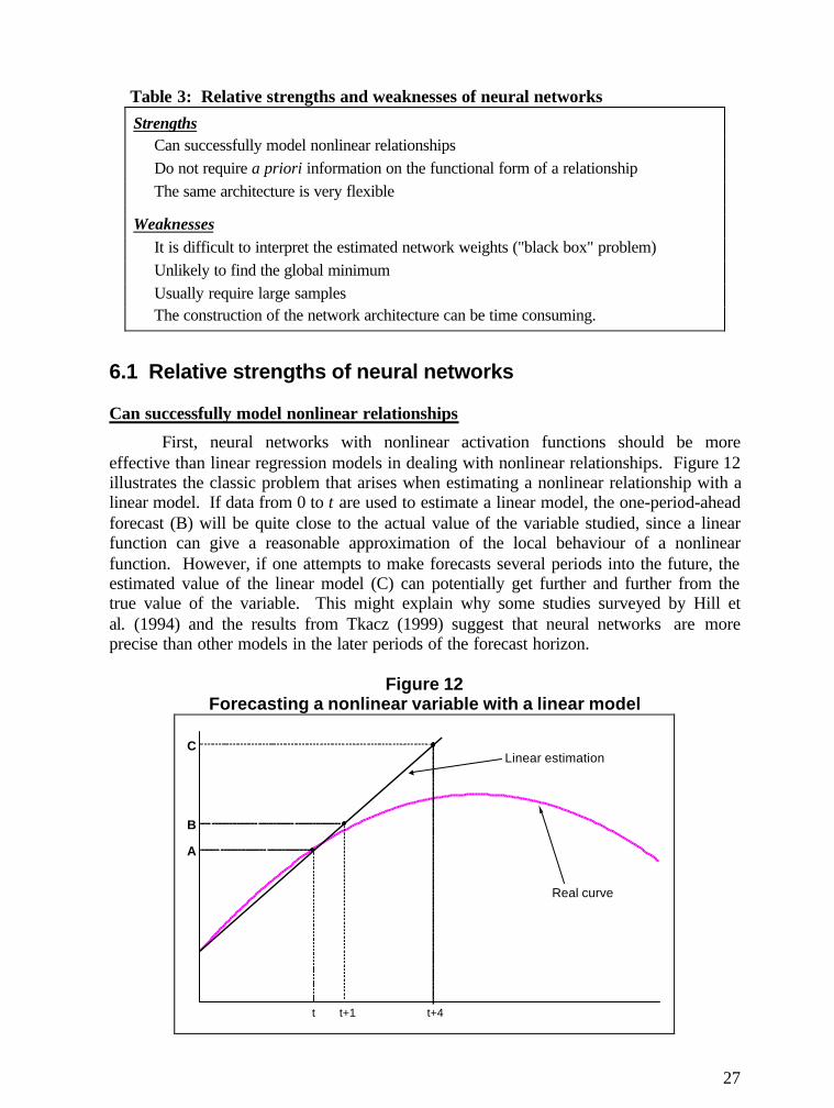
Can successfully model nonlinear relationships

First, neural networks with nonlinear activation functions should be moreeffective than linear regression models in dealing with nonlinear relationships. Figure 12illustrates the classic problem that arises when estimating a nonlinear relationship with alinear model. If data from 0 to t are used to estimate a linear model, the one-period-aheadforecast (B) will be quite close to the actual value of the variable studied, since a linearfunction can give a reasonable approximation of the local behaviour of a nonlinearfunction. However, if one attempts to make forecasts several periods into the future, theestimated value of the linear model (C) can potentially get further and further from thetrue value of the variable. This might explain why some studies surveyed by Hill etal. (1994) and the results from Tkacz (1999) suggest that neural networks are moreprecise than other models in the later periods of the forecast horizon.

Figure 12Forecasting a nonlinear variable with a linear model

t t+1 t+4

B

C

A

Real curve

Linear estimation

28

Do not require a priori information on the functional form of a relationship

Although many nonlinear functions can be linearized using relatively simplemathematical transformations, this supposes that the researcher has some a prioriknowledge of the nature of the nonlinearity that enables him to identify the appropriatetransformation to apply to the data. Needless to say, such information is rarely availablein the field of macroeconomic forecasting.

One could argue that nonlinear regression techniques would perform as well asneural networks when dealing with a nonlinear phenomenon. In theory, this is absolutelytrue. However, in practice, the estimation of a nonlinear regression model requires theeconometrician to assume an a priori functional form for the relationship studied.Selecting the wrong functional form will lead to imprecise coefficient estimates and badforecasts. On the other hand, when estimating a neural network, the researcher does notreally need to worry about the functional form of the phenomenon studied because the"universal approximator" property of networks will allow it to mimic almost anyfunctional form. No a priori knowledge is necessary to obtain precise forecasts.

The same architecture is very flexible

A third advantage of neural networks stems from the relative flexibility ofnetwork architectures. As illustrated at the beginning of this paper, a wide spectrum ofstatistical techniques (e.g. linear regression, a binary probit model, autoregressive models,etc.) can be specified by simply making minor modifications to the activation functionsand the network structure (such as changing the number of units in each layer). The samebasic architecture is therefore very flexible and can accommodate both discrete andcontinuous dependent variables.

6.2 Weaknesses and limitations of neural networks

It is difficult to interpret the estimated network weights ("black box" problem)

The complex nonlinear functional form of the network makes it very difficult tointerpret the estimated network weights. In linear regression models, the values of theestimated coefficients provide a direct measure of the contribution of each variable to themodel's output. In the case of neural networks, it is very complicated to analyticallyidentify the impact of an input on the estimated output value. Even in the simplest ofnetworks, such as in Figure 5, each input is fed through a nonlinear activation functionand is also affected by two different weights (aij and bj). Looking at equation (10), it isvery difficult to trace the impact of either X1 or X2 on Y. Because of these difficulties,neural networks are sometimes called "a black box": the network uses the inputs tocalculate the output, but the researcher does not clearly understand why a given value isforecasted. It must be noted that this problem can be greatly alleviated by applying thesensitivity analysis proposed by Refenes, Zapranis and Francis (1994). This procedurewill be discussed in Section 6.3.

29

Unlikely to find the global minimum

As with all nonlinear estimation methods, it is difficult to find the globalminimum of the error function. According to Goffe, Ferrier and Rogers (1994), anestimation problem with 35 weights (such as the network developed in Section 4) couldyield several quintillion local minima. Nonetheless, some local minima could producevery accurate forecasts if they are reasonably close to the global minimum.

Usually require large samples

A relatively simple neural network can contain a large number of weights. Insmall samples, this leaves a limited number of degrees of freedom, which will often leadto an overfitting of the training set, even when the early stopping procedure is used. Infact, the early stopping procedure can exacerbate this problem because it requires that thesample be split into three data sets, thus limiting the number of observations available forestimation and out-of-sample forecasting. For researchers interested in forecasting thedaily price of gold, data availability is not a problem because of the high frequency natureof the data. However, as shown in Section 4, an economist might encounter dataconstraints when attempting to forecast quarterly macroeconomic variables. Some of thestudies mentioned earlier were nonetheless able to successfully forecast macroeconomicvariables using relatively small samples. Our example from Section 4 also achieved acertain degree of success despite a modest sample size. Hence, the large-samplerequirement of neural networks does not seem to constitute an insurmountable problem.

The construction of the network architecture can be time consuming

As explained above, the network architecture must be designed by trial and error.Even though this process can be greatly shortened by programming the software packageto evaluate several architectures and by using a linear regression model to accelerate thechoice of network inputs (cf. Section 4.4), the designing and estimation of a network isstill considerably longer than in the case of a linear model.

6.3 A possible cure for the black box problem

As mentioned previously, neural networks are often called a "black box" becauseof the difficulty in establishing the direct relationship between a given input and theoutput. To address this issue, Refenes, Zapranis and Francis (1994) designed a simplebut effective way of assessing the sensitivity of the output to each input. Their methodconsists in charting the value of the output for a range of values of a given input 14, whileall other inputs are fixed at their sample mean. If the value of the output remainsrelatively stable for different values of the input in question (within a reasonable range),we can assume that this input does not contribute significantly to the predictive power ofthe network. By applying this process to all inputs, the researcher can better understandthe dynamics within the network and evaluate the contribution of each input to the

14 This procedure requires that each input be roughly bounded within a certain range. This is the case forvirtually all macroeconomic variables that are expressed as a growth rate.

30

estimated output value. The network can then be "pruned" through the elimination ofirrelevant inputs.

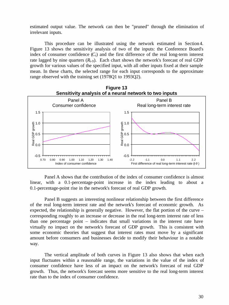
This procedure can be illustrated using the network estimated in Section 4.Figure 13 shows the sensitivity analysis of two of the inputs: the Conference Board'sindex of consumer confidence (Ct) and the first difference of the real long-term interestrate lagged by nine quarters (Rt-9). Each chart shows the network's forecast of real GDPgrowth for various values of the specified input, with all other inputs fixed at their samplemean. In these charts, the selected range for each input corresponds to the approximaterange observed with the training set (1978Q1 to 1993Q2).

Figure 13Sensitivity analysis of a neural network to two inputs

Panel A Consumer confidence

-0.5

0.0

0.5

1.0

1.5

0.70 0.80 0.90 1.00 1.10 1.20 1.30 1.40

Rea

l GD

P g

row

th

Index of consumer confidence

Panel B Real long-term interest rate

-0.5

0.0

0.5

1.0

1.5

-2.2 -1.1 0.0 1.1 2.2

Rea

l GD

P g

row

th

First difference of real long-term interest rate (t-9 )

Panel A shows that the contribution of the index of consumer confidence is almostlinear, with a 0.1-percentage-point increase in the index leading to about a0.1-percentage-point rise in the network's forecast of real GDP growth.

Panel B suggests an interesting nonlinear relationship between the first differenceof the real long-term interest rate and the network's forecast of economic growth. Asexpected, the relationship is generally negative. However, the flat portion of the curve –corresponding roughly to an increase or decrease in the real long-term interest rate of lessthan one percentage point – indicates that small variations in the interest rate havevirtually no impact on the network's forecast of GDP growth. This is consistent withsome economic theories that suggest that interest rates must move by a significantamount before consumers and businesses decide to modify their behaviour in a notableway.

The vertical amplitude of both curves in Figure 13 also shows that when eachinput fluctuates within a reasonable range, the variations in the value of the index ofconsumer confidence have less of an impact on the network's forecast of real GDPgrowth. Thus, the network's forecast seems more sensitive to the real long-term interestrate than to the index of consumer confidence.

31

Given the nonlinear nature of the network forecasts, the sensitivity of the outputto each input will change when the values of the other inputs are modified. Fixing theother inputs at their sample mean is somewhat arbitrary. The researcher can thereforeexperiment by fixing the other inputs at different values. In particular, the researcher canfix all other inputs at their current value (i.e. their value at the end of the sample) in orderto evaluate the imminent impact of a given scenario (e.g. if interest rates were to increasein the upcoming quarter).

In addition to this sensitivity analysis, a researcher may apply the optimal brainsurgeon (OBS) test, developed by Hassibi and Stork (1993), to prune the network. TheOBS test is essentially a Wald test that allows the researcher to assess if a given weight issignificantly different from zero. Hence, the researcher may gain even more insight intothe internal dynamics of the model and eliminate superfluous connections from thenetwork.

6.4 A few myths about neural networks

The growth in popularity of neural networks in recent years has led someresearchers to make partial judgements in favour or against these models. In this section,we will review a few of these claims (Table 4).

Table 4: Pseudo-strengths and pseudo-weaknesses of neural networksPseudo-strengths

Networks do not require the type of distributional assumptions used in econometricsNetworks are intelligent systems that learn

Pseudo-weaknessesThe architecture of a neural network is totally unrelated to economic theoryThe early stopping procedure requires arbitrary decisions by the researcher

6.4.1 Pseudo-strengths of neural networks

Networks do not require the type of distributional assumptions used in econometrics

Some researchers, such as Aiken and Bsat (1999), claim that neural networks arenot constrained by the distributional assumptions used in other statistical methods.However, as demonstrated by Sarle (1998), neural networks involve exactly the sametype of distributional assumptions as other statistical methods. For more than a century,statisticians have studied the properties of various estimators and have identified theconditions under which these estimators are optimal, i.e. when they yield consistentunbiased estimates with a minimal variance. They discovered, for example, that optimalresults are obtained when the errors have a zero mean, are uncorrelated with each other,and have a constant variance throughout the sample. By rigorously identifying theseoptimality conditions, statisticians have been able to assess the consequences of theviolation of these conditions. Since many neural networks are equivalent to statistical

32

methods, they require the exact same conditions to attain an optimal performance. Thisimplies, among others, that the residuals of a neural network should be subjected to thesame diagnostic tests that are applied to the residuals of a linear regression model.Researchers who ignore these optimality conditions and proceed to estimate their networkweights will obtain sub-optimal estimates. Most empirical studies involving neuralnetworks do not pay attention to these optimality conditions.

Unfortunately, the literature does not contain any thorough investigation of thestatistical properties of the neural network estimators. In particular, it would beworthwhile to develop a greater understanding of the variance of the network weights,which could be used to assess the variance of the network forecasts.

Moreover, researchers also tend to ignore issues of stationarity when buildingtheir network. A prudent researcher should verify that all variables in the network arestationary before experimenting with different architectures. In fact, level variables thatare trend stationary but that are not bounded could also pose problems for the network.Since a hidden unit produces a value that is bounded, the use of input variables that growcontinuously over time could eventually lead the hidden units to reach their maximal orminimal value. The contribution of each hidden unit to the network's output (which isgiven by the value of the hidden unit multiplied by the weight connecting it to the outputunit) would then remain constant, even if the boundless input continues to grow overtime. This would result in a deterioration of forecasting accuracy for subsequentperiods15. Similar problems would arise when attempting to forecast a level variable thatgrows continuously over time. Hence, even trend stationary level variables should betransformed so that they do not grow continuously over time (e.g. by using the firstdifference, the growth rate, the ratio to GDP, etc.)

Networks are intelligent systems that learn

Many researchers place great emphasis on the ability of feedforward neuralnetworks to "learn" relationships from a set of variables. They are therefore credited asbeing "intelligent" systems. In reality, the so-called "learning" ability of feedforwardneural networks is simply the result of applying an algorithm to minimize an errorfunction in order to fit the network output to a given data series. As such, these networksdo not have any additional "learning" capabilities than say, a linear regression model.Both methods simply extract correlations from the data to approximate the behaviour of agiven variable. The terms "learning" and "intelligent", probably borrowed from theresearchers in the field of artificial intelligence that invented neural networks, tend tocreate confusion as to the true capabilities of these models.

15 It is important to note that an augmented network's output is not bounded. The linear terms included inthe network would still allow its forecast to grow continuously over time, but the network would loose itsnonlinear properties once all hidden units reach their boundary.

33

6.4.2 Pseudo-weaknesses of neural networks

The architecture of a neural network is totally unrelated to economic theory

In econometrics, it is standard practice to choose a functional form that is basedon a theoretical model. However, when working with neural networks, the same basicfunctional form (e.g. equation [10]) will be used for a variety of heterogeneousapplications, from forecasting quarterly real GDP growth to predicting the daily price ofIBM ordinary shares. The "atheoretical" nature of the neural network functional formcould thus be viewed as a weakness to this approach.

However, one must remember that the functional forms used in theoreticaleconomic models are chosen quite arbitrarily. Economic theory only providesinformation on the explanatory variables to be considered and not on the functional formof a relationship. Although the actual functional form used in a theoretical model ischosen based on certain characteristics that are consistent with economic theory – such asbeing concave or convex, bounded or unbounded, etc. – economic theory itself does notspecify any functional form. The lack of theoretical underpinnings in the selection of thefunctional form is a problem inherent to all empirical analyses in economics, not justneural networks.

The early stopping procedure requires arbitrary decisions by the researcher

When implementing the early stopping procedure, the researcher must make acertain number of arbitrary decisions that can have a significant bearing on the estimationresults. First, the researcher must divide the sample into training, validation and test sets.A commonly used "rule of thumb" consists in retaining 25 per cent of the sample for thevalidation set and an equal proportion for the test set, with the remainder being allocatedto the training set. However, this guideline does not have any theoretical or empiricalfoundations. In addition, the researcher must decide which observations to include ineach set. Some researchers assemble their validation set from the most recentobservations in their time series, while others randomly select observations from theentire sample. Once again, there is no objective rule to this effect.

These criticisms should not be overemphasized since a researcher can estimate thenetwork using different allotments of the data into the various sets and thus assess thesensitivity of the results to this allotment. Moreover, it is important to remember thateconometricians make similar arbitrary decisions when they withhold observations fromtheir sample in order to make out-of-sample forecasts. Econometricians using time-seriesdata typically withhold an arbitrary number of observations from the end of their sample,since they are interested in assessing the model's capacity to forecast the future. To theextent that researchers in the neural network field assemble their validation and test setsfrom the last observations of the sample, they will be consistent with standardeconometric practice.

34

7. CONCLUSION: ARE NEURAL NETWORKS RELEVANT FORMACROECONOMIC FORECASTING?

The success of some of the studies described above and of the example developedin Section 4 suggest that some macroeconomic variables lend themselves to accurateforecasting with neural networks. These results also suggest that the four weaknessesdiscussed above do not seem to pose insurmountable obstacles to the effective use ofneural networks.

Ultimately, neural networks will be able to improve on linear models if therelationships studied present significant nonlinearities. Although some of the studiessurveyed by Hill et al. (1994) concluded that neural networks were more accurate forhigh frequency data, we would argue that these results were obtained only because thespecific time series used in those studies exhibited more nonlinearities in their highfrequency format and because the large samples available with high frequency datareduced the problem of overfitting16. Thus, those results may have had less to do with thedata frequency than with the fundamental characteristics of the data set.

Neural networks should be viewed as a natural complement to the linearregression model. Researchers interested in constructing a neural network would benefitfrom using their best linear model as a starting point. As explained in Section 4.4, alinear regression model should be used to help choose the network inputs. Additionally,a researcher can use the estimated coefficients from the linear model as starting values forthe augmented terms in the network (with the other weights being randomized at verysmall values). By proceeding in this way, we can maximize the probability of finding anetwork that will perform better than the linear model.

It is only after this avenue has been explored that the researcher should considermaking more substantial departures from the linear model, such as using inputs that werenot significant in the linear estimations. In the case of variables that can be accuratelyforecasted with linear models, the gains from departing from the linear model are likelyto be small, as the data generating process probably contains few nonlinearities. In thecase of variables that are not easily modelled with a linear equation, the researcher mighthave to experiment with networks that depart significantly from the linear model.

Overall, neural networks seem to have some potential to assist economists in theirmacroeconomic forecasting. At the very least, they deserve to be studied further, perhapsthrough forecasting competitions with other methods. It is only by implementing neuralnetworks in a specific context that economists will be able to evaluate their true potential.

Obviously, acquiring the expertise to implement a high-quality neural networkwould involve a substantial investment in time and effort. This investment could be 16 We see no reason to believe that all time series will necessarily exhibit more nonlinearities when they aremeasured in higher frequencies. However, at high frequencies, some financial series have a non-gaussianconditional distribution and some also exhibit an asymmetric behaviour that could be better captured byneural networks. This remains an empirical issue.

35

justified only if the potential gains from improved forecasting accuracy outweigh theinvestment required to implement the network. This will generally be true in the case ofmacroeconomic variables for which there is a lot of room for improved forecasting, i.e.variables that give rise to substantial forecasting errors with existing techniques(commodity prices might represent a good candidate in that respect). This would also betrue for variables that are of such great importance that even a marginal improvement inforecasting accuracy would be desirable. This could be the case for nominal GDP growthor interest rates, which have far-reaching implications for the design of fiscal andmonetary policies.

36

REFERENCES

Aiken, Milam (1999): "Using a Neural Network to Forecast Inflation", IndustrialManagement and Data Systems.

Aiken, Milam and Bsat, Mohammad (1999): "Forecasting with Neural Networks",Information Systems Management.

Andersson, Tomas and Falksund, Victoria (1994): "Using Neural Nets to Analyse GlobalMarkets", AI in Finance, Fall 1994, p.7-17.

Armstrong, Larry and Gross, Neil (1998): "Ford Slips a Neural Net Under the Hood",Business Week, Issue 3597, September 28, 1998, p. 81.

Ashley, R.; Granger, C.W.J. and Schmalensee R. (1980): "Advertising and AggregateConsumption: An Analysis of Causality", Econometrica, Vol. 48, No. 5(July 1980), p. 1149-1167.

Bramson, M.J. and Hoptroff, R.G. (1990): "Forecasting the Economic Cycle: A NeuralNetwork Approach", paper presented at the Workshop on Neural Networks forStatistical and Economic Data, Dublin, 10-11 December, 1990.

Brecht, Bennett C. and Aiken, Jim (1995): "A Lot of Nerve", Keyboard Magazine, June1995.

Chatfield, Chris (1993): "Neural networks: Forecasting Breakthrough or Passing Fad?",International Journal of Forecasting 9, p.1-3.

Chong, Y.Y. and Hendry, D.F. (1986): "Econometric Evaluation of LinearMacroeconomic Models", Review of Economic Studies, 53, p.671-90.

Church, Keith B. and Curram, Stephen P. (1996): "Forecasting Consumers' Expenditure:A Comparison between Econometric and Neural Network Models,"International Journal of Forecasting, 12, p.255-267.

Cybenko, G. (1989): "Approximation by Superpositions of a Sigmoid Function,"Mathematics of Control, Signals, and Systems 2, p.303-314.

Diebold, Francis X. and Mariano, Roberto S. (1995): "Comparing Predictive Accuracy",Journal of Business and Economic Statistics, Vol. 13, No. 3 (July 1995),p.253-263.

37

Domowitz, I. and White, Halbert (1982): "Misspecified Models with DependentObservations," Journal of Econometrics 20, p.35-58.

Donaldson, Glen R. and Kamstra, Mark (1996): "Forecast Combining with NeuralNetworks", Journal of Forecasting, Vol. 15, p.49-61.

Funahashi, K. (1989): "On the Approximate Realization of Continuous Mappings byNeural Networks," Neural Networks 2, p.183-192.

Fauvel, Yvon; Paquet, Alain and Zimmermann, Christian (1999): "A Survey on InterestRate Modelling and Forecasting," Working Paper of the Centre for Researchon Economic Fluctuations and Employment (CREFE), Université du Québec àMontréal, March 1999.

Fu, Jiarong (1998): "A Neural Network Forecast of Economic Growth and Recession,"The Journal of Economics, XXIV, No. 1, p.51-66.

Gallant, A.R. and White, Halbert (1988): A Unified Theory of Estimation and Inferencefor Non-linear Dynamic Models. Oxford: Basil Blackwell.

Gibb, Jondarr (1996): "Back Propagation Family Album", Technical Report C/TR96-05,Macquarie University, August 1996.

Goffe, William L; Ferrier, Gary D. and Rogers, John (1994): "Global Optimization ofStatistical Functions with Simulated Annealing", Journal of Econometrics,Vol. 60, p.6s-99.

Hassibi, B. and Stork, D.G. (1993): "Second Order Derivatives for Network Pruning:Optimal Brain Surgeon," in Hanson, Stephen José; Cowan, Jack D.; and Giles,C. Lee editors, Advances in Neural Information Processing Systems, 5,p.164-171, Morgan-Kaufmann, San Mateo, CA.

Hill, Tim; Marquez, Leorey; O'Connor, Marcus and Remus, William (1994): "ArtificialNeural Network Models for Forecasting and Decision Making", InternationalJournal of Forecasting, 10, p.5-15.

Hornik, K.; Stinchcombe, M. and White, Halbert (1989): "Multi-Layer FeedforwardNetworks Are Universal Approximators," Neural Networks 2, p.359-366.

Hornik, K.; Stinchcombe, M. and White, Halbert (1990): "Universal Approximation of anUnknown Mapping and Its Derivatives Using Multilayer FeedforwardNetworks," Neural Networks 3, p.551-560.

38

Kuan, Chung-Ming and White, Halbert (1994): "Artificial Neural Networks: AnEconometric Perspective", Econometric Reviews, 13(1), p.1-91.

Lamy, Robert (1999): "Finance Indicator Models: Short-Term Outlook for Growth,Inflation and the Business Cycle", Finance Canada, internal document.

LeCun, Y.; Boser, B.; Denker, J.S.; Henderson, D.; Howard, R.E.; Hubbard, W. andJackel, L.D. (1990), "Backpropagation Applied to Handwritten Zip CodeRecognition.", Neural Computation, 1, p.541-551.

Lim, Tjen-Sien; Loh, Wei-Yin and Shih, Yu-Shan (1998): "An Empirical Comparison ofDecision Trees and Other Classification Methods", Technical Report 979,Department of Statistics of the University of Wisconsin, Madison, January 27,1998.

McCann, Peter J. and Kalman, Barry L. (1994): "A Neural Network Model for the GoldMarket", working paper of the Department of Computer Science, WashingtonUniversity.

McMenamin, Stuart J. (1997): "A primer on neural networks for forecasting", Journal ofBusiness Forecasting, Vol. 16, Fall 1997, p.17-22.

Moody, John; Levin, Uzi and Rehfuss, Steve (1993): "Predicting the U.S. index ofindustrial production", Neural Network World, 3(6), p.791-794 in special issue:Proceedings of Parallel Applications in Statistics and Economics '93, MirkoNovak (ed.).

Refenes, Apostolos Nicholas; Zapranis, Achileas and Francis, Gavin (1994): "StockPerformance Modelling Using Neural Networks: A Comparative Study WithRegression Models", Neural Networks, Vol. 7, No. 2, p.375-388.

Sarle, Warren S. (1994): "Neural Networks and Statistical Models", Proceeds of theNineteenth Annual SAS Users Group International Conference, April 1994.

Sarle, Warren S. (1995): "Stopped Training and Other Remedies for Overfitting",Proceedings of the 27th Symposium on the Interface, 1995.

Sarle, Warren S. (1998): "Neural Network FAQ, part 1: Introduction", monthly postingon the Web site of the SAS Institute at ftp://ftp.sas.com/pub/neural/FAQ.html,May 1998.

39

Sejnowski, T. and Rosenberg, C. (1986): "NETalk: A Parallel Network That Learns toRead Aloud", John Hopkins University Department of Electrical Engineeringand Computer Science, Technical Report 86/01.

Stinchcombe, M. and White, Halbert (1989): "Universal Approximation UsingFeedforward Networks With Non-Sigmoid Hidden Layer ActivationFunctions," Proceedings of the International Joint Conference on NeuralNetworks, San Diego. New York: IEEE Press, p. I:612-617.

Stock, James H. and Watson, Mark W. (1998): "A Comparison of Linear and Nonlinearunivariate models for Forecasting Macroeconomic Time Series," NationalBureau of Economic Research Working Paper 6607, June 1998.

Swanson, Norman R. and White, Halbert (1995): "A Model-Selection Approach toAssessing the Information in the Term Structure Using Linear Models andArtificial Neural Networks," Journal of Business and Economic Statistics, July1995, Vol. 13, No. 3, p.265-275.

Swanson, Norman R. and White, Halbert (1997): "A Model Selection Approach to Real-Time Macroeconomic Forecasting Using Linear Models and Artificial NeuralNetworks", Review of Economics and Statistics, 79, November 1997,p.540-550.

Tal, Benny and Nazareth, Linda (1995): "Artificial Intelligence and EconomicForecasting", Canadian Business Economics, Spring 1995, p.69-74.

Tamura, Shin'ichi and Tateishi, Masahiko (1997): "Capabilities of a Four-LayeredFeedforward Neural Network: Four Layers Versus Three", in IEEETransactions on Neural Networks, Vol. 8, No. 2, March 1997.

Tesauro, G. (1989): "Neurogammon Wins Computer Olympiad," Neural Computation 1,p.321-323.

Tkacz, Greg (1999): "Neural Network Forecasts of Canadian GDP Growth UsingFinancial Variables," Bank of Canada, mimeo, April 1999.

Verkooijen, William (1996): “A Neural Network Approach to Long-Run Exchange RatePrediction,” Computational Economics, 9, p.51-65

White, Halbert (1981): "Consequences and Detection of Misspecified NonlinearRegression Models," Journal of the American Statistical Association 76,p.419-433.

40

White, Halbert (1992): Estimation, Inference and Specification Analysis. New York:Cambridge University Press.

20002000-07 Networks for Macroeconomic Forecasting: A Complementary Approach to Linear Regression Models – Steven Gonzalez

2000-06 Forecasting employment Rates: A Cohort Approach – Marie-France Paquet and Timothy C. Sargent

2000-05 Measuring Human Capital in Canada - Mireille Laroche and Marcel Mérette of the University of Ottawa

2000-04 L’écart à terme comme indicateur de l’activité économique : L’expérience des années 90 Paul Delâge et Jean-François Fillion

2000-03 Croissance endogène et vieillissement démographique : le cas d’une petite économie ouverte* Maxime Fougère

2000-02 “Modeling Federal Finances under Uncertainty” Derek Hermanutz and Chris Matier

2000-01 “Liability Management Using Dynamic Portfolio Strategies” Richard Black, Colin R. Telmer

1999

99-03 “An Econometric Examination of the Impact of Population Ageing on Personal Savings in Canada” , Maxime Fougère - Finance, Marcel Mérette - University of Ottawa

99-02 “Analyzing and Forecasting Credit Ratings: Some Canadian Evidence” Patrick Sabourin

99-01 “Taxation and Economic Performance: A Cross-Country Comparison and Model Sensitivity Analysis” Jing Xu

1998

98-09 “The BU Ratio: Prospect and Retrospect” Timothy C. Sargent

98-08 “Youth and the 1990s Labour Market” Carolyn Wilkins

98-07 “The Canadian Economic and Fiscal Model – 1996 Version: Part 3 – Empirical Specificationand Statistical Assessment” Jian-Guo Cao and Benoît Robidoux

98-06 “The Canadian Economic and Fiscal Model – 1996 Version: Part 2 – Dynamic Forecasting andSimulation Properties” Alain DeSerres, Benoît Robidoux and Bing-Sun Wong

98-05 “The Canadian Economic and Fiscal Model – 1996 Version: Part 1 – Model Structure” BenoîtRobidoux and Bing-Sun Wong

98-04 “Population Ageing and the Current Account in Selected OECD Countries” Maxime Fougèreand Marcel Mérette

98-03 “Population Ageing and Economic Growth in Seven OECD Countries” Maxime Fougère andMarcel Mérette

98-02 “The Persistence of Low Income Spells in Canada, 1982-1993” Mireille Laroche

98-01 “On the Concept and Dimensions of Human Capital in a Knowledge-Based Economy Context”Mireille Laroche, Marcel Mérette and G.C. Ruggeri

1997

97-08 “Estimating the Economic Efficiency Consequences of Alternative Tax Reforms Using a CGE Model: Homogeneous Vs Heterogeneous Labour Specifications” Louis Beauséjour, Mokhtar Souissi, Carole Vincent and G.C. Ruggeri

97-07 “Tax Expenditures and Tax Preferences in the Personal Income Tax System of Selected OECD Countries: A Suggested Classification, G.C. Ruggeri and Carole Vincent

97-06 “Income Taxes, Life-Cycles and Growth”, Marcel Mérette

97-05 “Effective Income Tax Rates in Macroeconomics: An Update for Canada”, G.C. Ruggeri, Mireille Laroche and Carole Vincent

97-04 “A Public versus a Private Canada Pension Plan: A Survey of the Economics” Steven James

97-03 “Forecasting Canadian Recessions with Macroeconomic Indicators” Robert Lamy

97-02 “The Dynamic Effects of Taxes and Government Spending in a Calibrated Canadian Endogenous Growth Model” Jing Xu

97-01 “The Impact of Fiscal Policy on the Risk Premium of Government Long-Term Debt: Some Canadian Evidence” Todd Mattina and François Delorme

1996

96-06 “Does the Length of the Current Expansion Increase the Probability of Recession?” Lisa Backa

96-02 “Do Mechanical Filters Provide a Good Approximation of Business Cycles?”, Alain Guay and Pierre St-Amant

96-01 “An Indicator Model of Core Inflation in Canada” Robert Lamy and Paul Rochon

1995

95-12 “Potential Economic Effects of Experience-Rating the Unemployment Insurance System Using a Multi-Sector General Equilibrium Model of Canada” Louis Beauséjour, Munir A. Sheikh and Baxter Williams

95-11 “Active Labour Market Policies: An Evaluation” Lori Marchildon

95-10 “An Index of Unemployment Insurance Disincentives” Timothy C. Sargent

95-09 “The Economics of Canada Pension Plan Reforms” Steven James, Chris Matier, Humam Sakhnini and Munir Sheikh

95-08 “The Long-Run Economic Impacts of Government Debt Reduction” Steven James and Chris Matier

95-07 “Time Series Properties of Canadian Real Interest Rates”, Chris Matier and Werner Schüle

95-06 “Interpreting Sacrifice Ratios Across Countries and Over Time” Brenda Lipsett and Steven James

95-05 “Effective Rates of Assistance: An Old Idea Whose Time Has Come?” Louis Beauséjour and Munir A. Sheikh

95-04 “Aggregate Fluctuations, Monetary Policy and Nominal Wage Rigidities in a New-Classical Setting: Results for Canada” Humam Sakhnini

95-03 “Ricardian Equivalence and the Permanent Income Hypothesis: An Empirical Investigation”Benoit Perron

95-02 “Are New-Classical Models Becoming Relevant Policy Tools: A Survey of Recent New- Classical Models” Humam Sakhnini

95-01 “Fluctuations économiques dans un environnement de stabilité des prix” Claude LavoiePlease note that this working paper is available in French only.

1994

94-06 “Conditional Productivity Convergence in Canada” Frank C. Lee

94-05 “A Guide to Applied Modern Macroeconometrics” Alain Paquet

94-04 “Interindustry Wage Differentials: Evidence, Explanations and Potential Distortions” Mario Iacobacci

94-03 “Regional Productivity Convergence in Canada” Frank C. Lee and Serge Coulombe

94-02 “Regional Economic Disparities in Canada” Serge Coulombe and Frank C. Lee

94-01 “The Interaction of Inflation with a Canadian-Type Capital Tax System: A Dynamic General Equilibrium Analysis Incorporating Endogenous Leverage and Heterogeneous Households” Steven James

1992

92-04 “An Environmental CGE Model of Canada and the United States” Louis Beauséjour, Gordon Lenjosek and Michael Smart

92-03 “Estimating Trend Total Factor Productivity Growth in Canada” Carolyn Wilkins, Frank Lee and Steven James

92-02 “Un indice de prix régional de biens et services comparables au Canada et son application aux disparités régionales de revenu” Raynald Létourneau. Available in French only.

92-01 “A New Composite Leading Indicator of the Canadian Economy” Robert Lamy

1990

90-07 “Une analyse empirique des déterminants du taux d'intérêt réel mondial” Benoît RobidouxPlease note that this working paper is available in French only.

90-06 “Real Interest Rates in Historical Perspective” Paul Jenkins

90-05 “The Contribution of Fiscal Policy to Real Interest Rate Movements in the 1980s” Paul Jenkins

90-04 “The Constant Price Hypothesis in Multi-Industry Cross-Section Studies: The Impact on Cost Function Estimates” Benoît Robidoux and John Lester

90-03 “The Cyclically-Adjusted Output Methodology” Mario Albert, Nathalie Boisvert and Robert Fonberg

90-02 “The Determination of Real Interest Rates” Joel Fried and David Burgess

90-01 “La voie des dépenses fiscales : le point sur les questions conceptuelles et les controverses”Neil Bruce. Available in French only.

1989

89-07 “INTERMOD 2.0: Model Specification and Simulation Properties” Guy Meredith

89-06 “The Calculation of Marginal Effective Tax Rates in the 1987 White Paper on Tax Reform”Jack Jung

89-05 “Effects of Changing Age Structure on Consumption and Saving” Paul Jenkins

89-04 “Expectations, Policy Shocks, and Output Behaviour in a Multi-Country Macroeconomic Model”

Guy Meredith

89-03 “The Goods and Services Tax: A General Equilibrium Analysis” Bob Hamilton and Chun-Yan Kuo

89-02 “A Survey of Some Recent Developments in Macroeconomics” Michael Devereux

89-01 “Closed Economy Analysis of the Dynamics of Deficits and Debt in a Unitary and Federal State” - Carolyn Wilkins and Mario Albert

1988

88-10 “A Guide to the GET Model” Richard G. Harris

88-09 “INTERMOD Model User's and Developer's Guide for PC Systems” Philip Bagnoli and Anders Kruus

88-08 “The Trade Sector in INTERMOD” Guy Meredith

88-07 “INTERMOD 1.1: A G-7 Version of the IMF's Multimod” John F. Helliwell, Guy Meredith, Yves Durand and Philip Bagnoli

88-06 “Resolutions of the U.S. Trade Imbalances: How Painful Will the Adjust Be?” Janice Haritos

88-05 “Econometric Estimates of Import Price Elasticities for Canada” Raynald Létourneau and John Lester

88-04 “Econometric Estimates of Scale Economies in Canadian Manufacturing” Benoît Robidoux and John Lester

88-03 “Trade Barriers Between Canada and the United States” John Lester and Tony Morehen

88-02 “New Estimates of Canadian Tariff Rates by Industry and Commodity” John Lester and Tony Morehen

88-01 “Geographic Labour Mobility in Canada” Louis Grignon and Kei Moray

1987

87-01 “Économies d'échelle : Un survol des techniques d'estimation et des problèmes méthodologiques”

Benoît Robidoux. Available in French only.1986

86-01 “The Structure of Production in Ten Canadian Industries” François Delorme and John Lester