Equity Valuation An examination of which investment valuation method appears to attain

the closest value to the market price of a stock

Master’s Thesis within Business Administration

Author: Nathalie Söderlund

Tutor: Johan Eklund, Andreas Högberg

Jönköping June 2011

Master’s Thesis within Business Administration

Title: Equity Valuation – An examination of which investment valuation

method appears to attain the closest value to the market price of a

stock

Author: Nathalie Söderlund

Tutor: Johan Eklund, Andreas Högberg

Date: 2011-06-01

Subject terms: Equity valuation, Discount valuation models, Valuation Error

Abstract

PURPOSE- This paper empirically evaluate the ability among various types

of parsimonious equity valuation models in order to ascertain which model

represents the value of equity the best and thereby manage to withstand fac-

tors causing valuation errors. The more complicated models applied, the

more underlying assumptions are needed. The trade-off here, which will be

investigated, is if the benefit of using more difficult models outweighs the

cost of including the extra assumptions. Further on the empirical research´s

results will be compared with the results provided by this previous studies

examinating American companies.

METHOD- Six valuation models using a discounting valuation method are

evaluated; the Present Value of Expected Dividends (PVED), Residual In-

come Valuation (RIV), Residual Income Valuation Terminal Value Con-

strained [RIV(TVC)], Abnormal Earning Growth approach (AEG), Abnor-

mal Earning Growth Terminal Value Constrained approach [AEG(TVC)]

and Free Cash Flow to the Firm model (FCFF). The five latter investment

models are all based on the first model.

FINDINGS- The aim of finding the smallest absolute valuation error in the

empirical study is given to PVED, a model including little underlying as-

sumptions and inputs. Hence, the implication of the application of valuation

models can be summarized as that there are no clear benefits of applying

complex models for Swedish companies, and the trade-off between using

more complex models and thereby including more assumptions is not com-

pelling given that the benefit does not exceed the cost. All the earnings

methods are all found to be superior to the FCFF model, while the con-

strained RIV and AEG methods provide higher valuation errors than the un-

constrained versions.

The superiority of the PVED model is inconsistent with the previous results

examining American firms, in which the RIV model is preferred. One of the

reasons for the difference is the use of different accounting standards in the

counties, and thereby the companies´ capital structure and the inputs used in

the investment valuation may be somewhat unlike.

Abbreviations

In order to simplify the notation, the following abbreviations are used;

Abs(V.E) = Absolute Valuation Error

AEG = Abnormal Earnings Growth model

AEG(TVC)= Abnormal Earnings Growth model Terminal Value Constrained

βSn = Equity beta for security n

Bvt = Book value of share at time t, after capital transactions at time t

Cbt = Conservative valuation bias at time t in equity of the company

Cov ( Sn,M ) = Covariance between security Sn and market portfolio (OMX30)

CSR = Clean surplus relation

D = The company´s amount of debt

Divt = The dividend paid out at time t

E = The company´s amount of Equity

EBIT = Earnings Before Interest and Tax

Et(…)= Expectation operator at time t

FCFF= Free Cash Flow to the Firm model

g = Company´s Growth rate in earnings in the steady state of the firm

GAAP = Generally Accepted Accounting Principles

HA = Alternative hypothesis

H&M= Hennes and Mauritz

HO = Null hypothesis

IFRS = International Financial Reporting Standards

k = Dividend payout ratio

Mi = Observation i for the market portfolio

N = Total number of observations

Pt = Price of the stock at time t, the market price

PVED= Present value of Expected Dividends (also called the dividend discount model)

PVEE= Present Value of Expected Earnings

PWC = Price Waterhouse Coopers

rD = Required rate of return by the debt holders

rE = Required rate of return of the equity holders

RE = rE + 1

rF = Risk free rate

RIV= Residual Income Valuation

RIV(TVC) = Residual Income Valuation Terminal Value Constrained

rM = Return of the market (based on the market portfolio)

rP = rF – rM, The market risk premium, i.e. the extra return required by investors for

holding a risky securities rather than a risk-free security

rwacc = Weighted Average Cost of Capital

Rwacc = rwacc + 1

SCA= Svenska Cellulosa Akitebolaget

SEB= Skandinaviska Enskilda Banken

Sn = Security n

T= Tax rate

UB = Unbiased accounting

Var(M) = Variance of the market

Var(Sn) = Variance of security n

V.E = Valuation Error

Vt = Value of the firm given by the investment model at time t

Xt = Accounting net earnings accumulated over the period

Yi = Observation i for security n

µSn = The mean for security n

ν = The mean of the market index

i

Table of Contents

1 Introduction .......................................................................... 3

1.1 Purpose ......................................................................................... 4 1.2 Background ................................................................................... 4

1.2.1 Investment models .............................................................. 5

1.2.2 Accounting standards ......................................................... 6 1.3 Previous research ......................................................................... 7 1.4 Method .......................................................................................... 8 1.5 Hypotheses ................................................................................. 10 1.6 Limitations of the study ................................................................ 11

1.7 Outline of the paper ..................................................................... 12

2 Investment valuation models ............................................. 13

2.1 Underlying assumptions for investment models used ................. 13 2.2 Discount rate ............................................................................... 13 2.3 Present Value of Expected Dividends, PVED ............................. 15

2.4 Earning´s models ........................................................................ 16 2.4.1 Residual Income Valuation, RIV ....................................... 16 2.4.2 Abnormal Earning Growth, AEG ....................................... 17

2.5 Free Cash Flow to Firm, FCFF .................................................... 18

3 Methodology ....................................................................... 20

3.1 Tax-rate, t .................................................................................... 20

3.2 Discount rates ............................................................................. 21

3.2.1 Risk-free rate, rF ............................................................... 21

3.2.2 Cost of equity, rE ............................................................... 21 3.2.3 Cost of debt, rD ................................................................. 22

3.3 Growth rate, g ............................................................................. 22 3.4 Modeling assumptions ................................................................. 23 3.5 Company information .................................................................. 23

3.5.1 Scania ............................................................................... 23 3.5.2 SCA .................................................................................. 24

3.5.3 Axfood .............................................................................. 24 3.5.4 H&M .................................................................................. 24 3.5.5 Tele2 ................................................................................. 24 3.5.6 SEB .................................................................................. 24

4 Empirical research ............................................................. 26

4.1 Summary of the companies ......................................................... 27 4.2 Present Value of Expected Dividends, PVED ............................. 28 4.3 Earning´s models ........................................................................ 29

4.3.1 Residual Income Valuation, RIV ....................................... 30 4.3.2 Residual Income Valuation Terminal Value Constrained, RIV(TVC) ............................................................... 31 4.3.3 Abnormal Earning Growth, AEG ....................................... 33 4.3.4 Abnormal Earning Growth Terminal Value Constrained, AEG(TVC) .............................................................. 34

4.4 Free Cash Flow to the Firm, FCFF .............................................. 35

5 Analysis and hypotheses testing ...................................... 37

ii

5.1 Testing hypotheses 1-6 ............................................................... 37 5.2 Testing hypothesis 7 ................................................................... 37 5.3 Testing hypotheses 8 - 11 ........................................................... 39

5.3.1 Residual Income Valuation, RIV ....................................... 39 5.3.2 Residual Income Valuation Terminal Value Constrained, RIV(TVC) ............................................................... 41 5.3.3 Abnormal Earning Growth, AEG ....................................... 43 5.3.4 Abnormal Earning Growth Terminal Value Constrained, AEG(TVC) .............................................................. 45 5.3.5 Results .............................................................................. 48

5.4 Testing hypothesis 12 ................................................................. 48 5.5 Testing hypotheses 13 & 14 ........................................................ 49

5.6 Fundamentals of companies ....................................................... 49

6 Discussion of empirical results ......................................... 51

6.1 Hypotheses and results ............................................................... 51 6.2 Company information and valuation bias .................................... 55 6.3 Swedish versus American companies ......................................... 56

7 Conclusion .......................................................................... 58

8 List of references ................................................................ 61

9 Appendix ............................................................................. 64

9.1 Appendix 1: Valuation errors in AEG(TVC) and RIV(TVC) .......... 64

9.2 Appendix 2: Valuation model´s result .......................................... 65

9.3 Appendix 3: Valuation errors and absolute valuation errors ........ 66

3

1 Introduction

_____________________________________________________________________________

Below is an introduction of investment valuation as well as a presentation of the problems

connected to the valuation process. The section also includes an outline of the study, which

helps address the problems and examines how previous research has approached the prob-

lems.

All assets can be assigned a value. In order to be successful in the market place as an

investor, one needs to understand not only the value of the asset, but also the primary

sources of value.

Deciding an assets value under uncertainty is difficult, since the value of an asset may

be ambiguous. Every year public listed companies need to produce financial statements,

helping analysts and investors understand the value of firms. Accounting is a phenome-

non created by humans but made up by regulations and laws, i.e. it is not something

naturally shaped. Even though the statements are created following regulations, they

should be used with caution. Managers can attempt to manipulate the statements in or-

der to make the company value larger so that the management´s options will be more

worth. Alternatively, if the managers make the company´s value on the financial state-

ments look less, “hidden” money can be collected. (Penman, 2001)

Making decisions under uncertainty is difficult, since the uncertainty may prevent the

investor to make an optimal choice. As an investor any reduction in uncertainty should

lead to better investment decisions. One way of trying to reduce uncertainty is to use in-

vestment valuation models before taking on an investment in order to find a price-worth

stock (French & Gabrielli, 2004). Investment valuation relates to when the fundamental

value of an investment is calculated, and various models exist. Valuation models that

require few assumptions and have a high ability to withstand strong impact of factors

are attractive to use.

The problem nowadays is not to find an investment model; it is to find the most appro-

priate one. What may strike as surprising are not the differences in the technique across

various assets, but the amount of relationships in the underlying principles in valuation.

(Damodaran, 2002)

The underlying idea behind the discount model is that the value of a stock can be found

by calculating a certain payoff back to present value (Damodaran, 2002). Most econo-

mists nowadays accept the usage of discounted valuation approach, but little empirical

evidence has been shown that using discounted investment model valuation actually

provides a correct valuation of the firm (Kaplan & Ruback, 1995). But which payoff to

discount in order to represent the most accurate value of equity is unclear, and will be

investigated in the empirical analysis.

The discount models rely on strong assumptions and the mechanical valuation technique

is sensitive for alterations in these assumptions. The more complicated discount models

used the more underlying assumptions. Hence, there is a trade-off here which will be

investigated; does the benefit of using more complex models outweigh the cost of the

extra assumptions needed to be included? What are the reasons and underlying assump-

tions causing the valuation bias?

4

1.1 Purpose

If perfect investment model existed, choosing the right securities for a portfolio would

be easy. The weakness of discounted cash flow models lie in deciding which payoff to

discount in order to reflect the value of equity the best. A perfect model has not yet been

found, but various investment models can be compared in order to ascertain the most

robust and appropriate model. According to the efficient market hypothesis, the market

price of a stock includes all available information (Elton, Gruber, Brown & Goetzmann,

2010). Even if the market is on average efficient, there are periods when the value of the

stock does not capture all information in the price and thereby over- or underpricing ap-

pears. By finding a model where the true equity value is reflected, periodic mispriced

stocks can be found and thereby investor can benefit from the mispricing.

The purpose of this research is to analyze which valuation model gives the best fore-

casted values compared to the actual market price. Hence, the investment models´ abil-

ity to withstand the factors causing valuation error will be empirically evaluated. The

primary idea behind this research is to compare the results provided by the various in-

vestment models to the market prices and observe how large valuation errors occur.

Further on important underlying assumptions and inputs will be introduced and exam-

ined in order to find out how these assumptions affect the models. What is the underly-

ing reason causing the model fail or work?

Previous studies have mostly exanimated American companies. The American compa-

nies are using General Accepted Accounting Principles (GAAP), while the Swedish

companies are using the somewhat different accounting standards, International Finan-

cial Reporting Standards (IFRS). The differences between IFRS and GAAP may create

somewhat different capital structure in the financial statements in the two countries,

leading to somewhat different inputs used in the investment valuation models. This will

be further investigated in order to find out if the accounting standards have any effect on

the choice of valuation method, and if Swedish companies prefer any other model com-

pared to the American firms.

Another area to investigate is if the information for a company not directly stated in the

numbers in the financial statements also affect the choice of investment models. Does

the age of the company play an important role? Are there other factors affecting the

market price?

The empirical research is supposed to help investors to chose the best security to invest

in by using the most appropriate investment model, thereby creating better investment

decisions. Hence, the results are supposed to help individuals to reduce uncertainty and

valuation errors when deciding which investment valuation model to use. The best

model also contributes with the best help when finding out whether stocks are currently

mispriced or not.

1.2 Background

In this section the background behind the investment models and the accounting stand-

ards are explained.

5

1.2.1 Investment models

There are various discount models suggesting which payoff to discount in order to rep-

resent the most accurate value of the company. Six different discount models are used in

the empirical study; Present Value of Expected Dividends (PVED), Residual Income

Valuation (RIV), Residual Income Valuation Terminal Value Constrained [RIV(TVC)],

Abnormal Earnings Growth (AEG), Abnormal Earnings Growth Terminal Value Con-

strained [AEG(TVC)] and Free Cash Flow to Firm (FCFF). For the five latter approach-

es PVED serves as a benchmark and thereby lays the foundation of the models (Skogvik

& Juettner-Nauroth, 2009).

The PVED model, also called the dividend discount model, was recognized by Williams

(1938, cited in Francis, Olsson, & Oswald, 2000). The model bases the value of the firm

on the future dividends (Francis, Olsson & Oswald 2000). This is the most commonly

used and simplest discount approach (Penman & Sougiannis, 1998).

Both RIV and AEG models have its roots in the clean surplus relation (CSR), claiming

that any modification in the book values will adjust the earnings and the dividends and

vice versa. Changes in book value between two periods are equal to the difference between

earnings and dividends. (Francis, Olsson & Oswald, 2000) Hence, changes in the share-

holder equity need to be stated in the income statement. The extra identification of value

leads to a separation between the creations of the wealth from the distribution of wealth.

(Ohlson, 1995)

The RIV model has its benchmark in the book value of owners’ equity, anchoring the

residual earnings to the firm´s creation of values. The current value of a stock is defined

by adding together the book value and the present value of the upcoming residual in-

come. (Skogsvik & Juettner-Nauroth, 2009)

The AEG model was recently introduced by Ohlson and Juettner-Nauroth (2005, cited

in Skogsvik and Juettner-Nauroth, 2009). The model starting points is the upcoming

earnings calculated to perpetuity added together with the present value of future abnor-

mal earnings growth (Skogsvik & Juettner-Nauroth, 2009).

Both RIV and AEG model has parsimonious versions where the terminal value is set to

zero at the horizon point of time, creating RIV(TVC) and AEG(TVC) models. The con-

strained models are more or less influenced by conservative accounting and company´s

distance to when a steady state at the horizon time is reached. (Skogsvik & Juettner-

Nauroth, 2009)

Together the RIV, RIV(TVC), AEG and AEG(TVC) model will be called the earnings

model, due to their recognition and inclusion of earnings.

The FCFF uses a more extensive approach compared to PVED. The model substitutes

the dividends into the free cash flow created by the firm, which represents the cash flow

available to all investors after reinvestment needs are subtracted. The amount of rein-

vestment measures how much is invested back to the firm in order to generate future

growth and earnings. The reinvestment rate can directly be connected to the dividend

payout ratio, since the more dividends are paid out the less is reinvested back into the

firm. The sum of the payout ratio plus the reinvestment rate must total one. (Damo-

daran, 2002)

6

1.2.2 Accounting standards

The effects of the accounting standard on the quality and quantity of information in the

financial statements cannot be dismissed. The accounting system used in Sweden, IFRS,

and in America, GAAP, includes accruals accounting (Penman, 2010). Accrual account-

ing refers to the fact that a company´s position is measured by recognizing economic

events regardless of when cash transactions occur. Matching revenues with expenses

when the transaction occurs rather than when the payment is made is supposed to pro-

vide a more accurate picture of a company's current financial situation.

Accounting conservatism refers to cautious use of the accounting principles when fi-

nancial statements are created, in the sense that

- The acquisition costs are written down more quickly than necessary to fair cost

matching principles.

- When operating assets and liabilities are valued in compliance with “lower his-

torical cost or market” and “higher of contractual obligation or market”.

- The unrealized losses in inventory and work-in-progress are recognized in the

financial statements while the unrealized profits and holding gains are not and

occur instead when can be foreseen.

- Positive net present value of current or future projects are not recognized in the

financial statements.

Conservative accounting focuses on the systematic bias in book value, created by the

principle of conservatism influence the setting and implementation of accounting stand-

ards. Assuming the CSR holds, the definition of conservative accounting concentrate on

the measurement bias of book value of owners´ equity, i.e. the financial and operating

assets subtracted by the financial and operating liabilities. (Skogsvik & Juettner-

Nauroth, 2009)

According to Feltham and Ohlson (1995) conservative and unbiased accounting are de-

fined in terms of how the book value differs on average from the market price.

Formula 1.1 Unbiased Accounting

Lim Et [BvT+t] / E [PT+t] = 1, regardless of date t information T→∞

The accounting policy is unbiased if the book value on average equals market price.

Formula 1.2 Conservative Accounting

Lim Et [BvT+t] / E [PT+t] < 1, regardless of date t information T→∞

Conservative accounting hence means that the book value is expected to be negatively

biased.

The conservative bias at time zero can be expressed with the formula;

Formula 1.3 Cb0

V0 – P0 = Bv0 – Bv0(UB)

= -Cb0

The formula above can be developed further and taking into account that the company is

acting in a steady state.

7

Formula 1.4 Cb0 and steady state company

Bv0 – Bv0(UB)

= Cb0 ≥ 0

E0 (Bvt(UB)

)-Bvt = E0 (Cbt) ≥ 0

E0 (Xt)= E0 [Xt(UB)

- (Cbt- Cbt-1)] = E0 (Xt(UB)

)- E0[ ∆(Cbt)]

The formula above implies that the market price of the stock is the same as the book

value of owners´ equity when the steady state is reached. However, one needs to re-

member that the effect of earnings is ambiguous. (Skogsvik & Juettner-Nauroth, 2009)

The RIV and AEG models are unaffected by conservative accounting (Penman 2006,

cited in Skogsvik & Juettner-Nauroth, 2009) while book value, PVED, RIV(TVC),

AEG(TVC) and FCFF are affected. Skogsvik and Juettner-Nauroth (2009) claim that if

the company is assumed to act in a steady state the valuation bias in the RIV(TVC) and

AEG(TVC) models are created from different sources. The valuation bias in the

RIV(TVC) model depends on the conservative bias of the value of equity at the horizon

time, while the valuation bias of the AEG(TVC) model depends on the capitalized

growth of the conservative bias in the terminal period. The valuation error for the

AEG(TVC) model will be less than the valuation error for the RIV(TVC) model if the

growth in the terminal period is small enough.

U.S. GAAP is generally considered to be more conservative than the IFRS due to the

controversial nature of the U.S. legal environment. U.S. accountants prefer clear rules in

decision making rather than subjective judgment. One example is how earnings can be

recognized. The GAAP require the money from the buyer is fixed or received, while the

IFRS require that the amount of earnings can be measured with reliability. (Ernst and

Young, 2009)

1.3 Previous research

Penman and Sougiannis (1998) made an empirical study of which payoff would give the

company the best valuation using ex post payoffs in discount models. The payoff used

by Penman and Sougiannis were dividends, cash flows and residual income. The securi-

ties consisted of portfolio combinations chosen from NYSE, AMEX and NASDAQ.

The time horizon examined contributed from one- to ten-years, and no matter which

horizon chosen the RIV approach turned out to be preferred compared to the dividend

model and the cash flow approach.

Francis, Olsson and Oswald (2000) investigate the same models as Penman and

Sougiannis above, but instead individual securities and forecasted data were used. Fore-

casted data contains unpredictable components which can confuse the evaluation be-

tween the valuation models. Francis, Olsson and Oswald’s results also indicate the su-

periority of the RIV model compared to the cash flow and dividend model. In both arti-

cles mentioned above the RIV model is referred to as the AE model.

Skogvik and Juettner-Nauroth (2009) instead evaluate the RIV and the AEG models

against each other. According to the authors’ results, the AEG(TVC) model provides

smaller valuation errors than the RIV(TVC) model if the growth in the terminal period

is small enough.

8

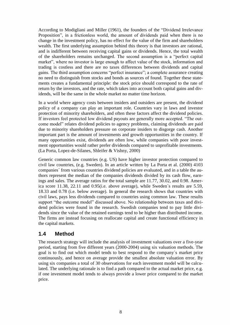
According to Modigliani and Miller (1961), the founders of the “Dividend Irrelevance

Proposition”, in a frictionless world, the amount of dividends paid when there is no

change in the investment policy, has no effect for the value of the firm and shareholders

wealth. The first underlying assumption behind this theory is that investors are rational,

and is indifferent between receiving capital gains or dividends. Hence, the total wealth

of the shareholders remains unchanged. The second assumption is a “perfect capital

market”, where no investor is large enough to affect value of the stock, information and

trading is costless and there are no taxes differences between dividends and capital

gains. The third assumption concerns “perfect insurance”; a complete assurance creating

no need to distinguish from stocks and bonds as sources of found. Together these state-

ments creates a fundamental principle: the stock price should correspond to the rate of

return by the investors, and the rate, which takes into account both capital gains and div-

idends, will be the same in the whole market no matter time horizon.

In a world where agency costs between insiders and outsiders are present, the dividend

policy of a company can play an important role. Countries vary in laws and investor

protection of minority shareholders, and often these factors affect the dividend policies.

If investors feel protected low dividend payouts are generally more accepted. “The out-

come model” relates dividend policies to agency problems, claiming dividends are paid

due to minority shareholders pressure on corporate insiders to disgorge cash. Another

important part is the amount of investments and growth opportunities in the country. If

many opportunities exist, dividends are often low, while companies with poor invest-

ment opportunities would rather prefer dividends compared to unprofitable investments.

(La Porta, Lopez-de-Silanes, Shleifer & Vishny, 2000)

Generic common law countries (e.g. US) have higher investor protection compared to

civil law countries, (e.g. Sweden). In an article written by La Porta et al. (2000) 4103

companies´ from various countries dividend policies are evaluated, and in a table the au-

thors represent the median of the companies dividends divided by its cash flow, earn-

ings and sales. The average ratios for the total sample are 11.77, 30.02, and 0.98. Amer-

ica score 11.38, 22.11 and 0.95(i.e. above average), while Sweden´s results are 5.59,

18.33 and 0.78 (i.e. below average). In general the research shows that countries with

civil laws, pays less dividends compared to countries using common law. These results

support “the outcome model” discussed above. No relationship between taxes and divi-

dend policies were found in the research. Swedish companies tend to pay little divi-

dends since the value of the retained earnings tend to be higher than distributed income.

The firms are instead focusing on reallocate capital and create functional efficiency in

the capital markets.

1.4 Method

The research strategy will include the analysis of investment valuations over a five-year

period, starting from five different years (2000-2004) using six valuation methods. The

goal is to find out which model tends to best respond to the company´s market price

continuously, and hence on average provide the smallest absolute valuation error. By

using six companies a total of 30 observations for each investment model will be calcu-

lated. The underlying rationale is to find a path compared to the actual market price, e.g.

if one investment model tends to always provide a lower price compared to the market

price.

9

The proposition that securities markets are efficient forms the basis for most research in

financial economics (Summers, 1986). Perfect market efficiency1 will be assumed,

thereby creating the assumption that the actual stock price represents the true value of

the equity since all information is incorporated in the price. Even if the market is effi-

cient and stocks are on average correctly priced, stocks may be mispriced during shorter

periods (Elton, Gruber, Brown & Goetzmann, 2010). By finding an investment where

the calculated value differs from the market price, over- and undervaluation of a stock

can be recognized and as an investor one can take advantage of the mispricing.

The numbers used as inputs are found in the firm’s financial statements and are realiza-

tions. Thereby, the assumption is made that the valuation errors between the market

prices and the investment models are results from the errors in the investment valuation

model. If there are continuously large gaps between the fundamental values and the cur-

rent market prices, examinations of the errors will be done in order to find out why the

errors arise and which of the underlying assumptions are causing the model to fail.

The study in this paper is an explanatory study since the link between the causes and re-

sults of the evidence are examined. In order to receive conclusions from the investment

valuation analysis, the results will be evaluated in Microsoft Excel2 using quantitative

research.

Information about the company and the accounting procedures used in order to perceive

the financial statement from which inputs are estimated will also be taken into account

in order to understand the results better. Thereby, qualitative research will also be used.

By using both qualitative and quantitative research, a better and clearer perspective is

received.

The investment valuation models examined was chosen mainly due to commonly occur-

rence in scientific articles (PVED, RIV and cash flow model). Further on, due to the

previous success of the RIV model which is an earnings model, another model basing

value on earnings were selected, the AEG model. Both the RIV and AEG have terminal

value constrained versions which also has been studied.

The investment valuation time period used is five years, due to the fact that previous

studies often have included this time frame (sometimes along with other time periods).

The companies chosen, Scania, Svenska Cellulosa Akitebolaget (SCA), Axfood,

Hennes and Mauritz (H&M), Tele2 and Skandinaviska Enskilda Banken (SEB), was se-

lected in order to include various sector and at the same time making sure that all com-

panies had been public listed since year 2000.

The empirical results can be sensitive to the sample selection. In this paper only six

companies from Stockholm’s exchange will be evaluated, and thereby potential sample

bias is possible. Reliability refers to the consistency of the measurement, and in order to

examine the reliability the variances of the models are represented as a measure of the

reliability. The more variance, the more deviations from the mean, and thereby the low-

er reliability of the model.

1 The market is efficient if the market price of a stock includes all available information (Elton, Gruber,

Brown & Goetzmann, 2010).

2 Statistical software

10

Validity is instead referred to as the strength of our conclusions, inferences or proposi-

tions. In order to capture how strong my test results are, three different significance lev-

els are used for the t-tests.

1.5 Hypotheses

In order to find out whether the null hypothesis will be accepted or rejected t-tests are

conducted basing the results on the pairs in the empirical research, using a paired t-test.

The market price and the calculated investment valuation result are considered as pairs.

The t-test relies on the assumption of normal distribution. By either comparing the p-

value with the significance level or the t-value with the critical t-value we can find out if

a significant difference exists. A low P-value corresponds to low likelihood of the null

hypothesis to be true. The first six hypotheses examines if there is a significant differ-

ence between the mean of the results and the mean of the market prices.

Hypothesis 1: there is no significant difference between the mean of the valuation error

results of the PVED model and the market prices.

Hypothesis 2: there is no significant difference between the mean of the valuation error

results of the RIV model and the market prices.

Hypothesis 3: there is no significant difference between the mean of the valuation error

results of the RIV(TVC) model and the market prices.

Hypothesis 4: there is no significant difference between the mean of the valuation re-

sults error of the AEG model and the market prices.

Hypothesis 5: there is no significant difference between the mean of the valuation error

results of the AEG(TVC) model and the market prices.

Hypothesis 6: there is no significant difference between the mean of the valuation error

results of the FCFF model and the market prices.

Hence, all the alternative hypothesis states there are a significant difference between the

means of the investment valuation model and the market price.

The FCFF model´s payoff represents what could be paid out as dividends, while PVED

discounts the actual dividends paid out. If the potential dividend is the same as the actu-

al, the two models provide the same result. Since companies do not always pay out

what they can afford in dividends, skewed estimates are possible. (Damodaran, 2002)

By comparing these two models one can investigate how much dividends represents the

market price the best. This will be further investigated in hypothesis 7.

Hypothesis 7: there is no significant difference between the mean of the absolute valua-

tion results of the FCFF model and PVED model.

Penman and Sougiannis (1998) and Francis, Olsson and Oswald´s (2000) results indi-

cate the RIV model provides less valuation bias compared to both FCFF and PVED.

This will be investigated further in hypotheses 8-11, including both the constrained and

unconstrained versions of RIV and AEG.

Hypothesis 8: RIV on average provides no significant difference in absolute errors re-

sults compared to both PVED and FCFF.

11

Hypothesis 9: RIV(TVC) provides no significant difference in absolute errors results

compared to both PVED and FCFF.

Hypothesis 10: AEG provides no significant difference in absolute errors results com-

pared to both PVED and FCFF.

Hypothesis 11: AEG(TVC) provides no significant difference in absolute errors results

compared to both PVED and FCFF.

Skogvik and Juettner-Nauroth (2009) claims the AEG(TVC) model provides smaller

valuation errors than the RIV(TVC). This will be further investigated in hypothesis 12.

Hypothesis 12: AEG(TVC) provides no significant absolute errors results compared to

RIV(TVC).

The constrained and unconstrained versions of RIV and AEG model will be compared,

in order to see whether including the terminal or not provides smaller valuation bias.

Hypothesis 13: RIV(TVC) provides no significant absolute errors results compared to

RIV.

Hypothesis 14: AEG(TVC) provides no significant absolute errors results compared to

AEG.

1.6 Limitations of the study

Strong assumptions and limited consistency of the data triggers discussion of the validi-

ty and robustness of the results. Since the investment valuation models require strict

treatment of accounting numbers and underlying assumptions, the results cannot be ex-

pected to fully hold in practice. The observed error variations in the statistical results

can generally be seen as robust over time and recognizing rules of thumb to apply on

companies has difficulties. Neither can one conclude which model is the best one for the

market nor that the model preferred is already used by the market and is with necessity

imprecise. Hence, the results from the empirical research cannot conclude if or which

model drives the price setting.

A perfect efficient market is assumed, but with awareness that there are limitations of

the perfect efficient market and the hypothesis is often questioned. Assuming market ef-

ficiency hold there is no idea to evaluate the firms, since all information is already re-

flected in the prices and thereby no stocks would be over- or underpriced on average.

But the underlying assumptions of market efficiency do not necessary hold, and even if

information would be available to everyone, there are costs of analysing and collecting

the data. (Grossman, Stiglitz 1980) If the securities in the market are not reflecting all

available information it is thereby possible to make investment valuation in order to find

over- and undervalued stocks (Summers, 1986).

The relationship between investor´s expectations and price movement of a stock is hard

to understand since fundamental values and investors´ beliefs are unobservable. Neither

can the factors be separated. As the market is repeated and as prices better reflect the

fundamentals, predictions starts to better correspond to fundamental values and thereby

prediction bias decreases. As long as the prices do not fully reflect the fundamentals and

are not perfectly efficient, traders´ expectations play an important role when predicting

future movements. The prediction bias is only absent when prices are tracking funda-

12

mentals. (Haruvy, Lahav, & Noussair, 2007) The companies selected for the empirical

research have been listed for more than ten years, which should lead to a smaller predic-

tion bias than selecting new companies, but may still exist.

Investment valuations models will in general do a poor job on firms not fitting into the

general frame. Examples of these types of companies are firms in trouble (the cash flow

does not represent the company´s true potential), cyclical firms, firms with nonutilized

assets, firms with patents and product options, firms in the process of reconstruction,

firms involved in acquisitions and private firms. If the company continuously loses

money, investment valuation models tend to do a poor job. (Damodaran, 2002) Stock-

holm OMX has 350 listed companies, but only 206 companies had positive net income

in 2009 (Bureau van Dijk, n.d.).

Companies are today acting in various countries, forcing the firms to cope with regula-

tions and laws from different countries and thereby additional economic, accounting and

legal issues need to be considered when analyzing their financial reports. Thereby, the

data might not be completely valid and comparable among the companies and countries.

When calculating the equity discount rate the CAPM (Capital Asset Pricing Model) is

used. The CAPM is often questioned due to the fact it is assumed the only factors af-

fecting the return for the investor is the market risk. The APT (Arbitrage Pricing Theo-

ry) is another approach used when calculating the discount rate which is more elaborat-

ed. This approach requires the return on any stock to be linearly related to a set of indi-

ces; hence it is a multi-index model looking to capture more of the explainability of why

investors want compensation for risk taken on. Examples of other factors affecting the

return of a stock according to the APT are e.g. inflation, term structure of interest rates,

risk premia and industrial production. APT theory provides a rate of return which repre-

sents a completer description of returns compared to the CAPM. The weakness of this

model is the fact that the indices which should be used are not specified. (Elton et al.,

2010) The CAPM formula is used in the articles written by Penman and Sougiannis,

(1998) and Francis, Olsson, and Oswald (2000). The reason for larger possibility for bi-

as in this paper is the fact that fewer companies are used. The larger amount of compa-

nies the larger possibility that the errors cancel each other out.

1.7 Outline of the paper

The outline of the paper is as follows: the next section discusses investment valuation

models and its assumptions. In section three, the inputs are explained how forecasted.

Analysis and discussion of the results are presented in section four and five respective-

ly. In closing, concluding remarks are high- lighted, followed by further possible stud-

ies. The appendices provide explanatory tables and information.

13

2 Investment valuation models

_____________________________________________________________________________

This chapter present the theory behind investment valuation methods. This information will

further be taken into account in the empirical studies in order to conduct appropriate anal-

ysis.

As told above, all assets, no matter financial or physical, have value. The key to be a

successful investor lies in the way of understanding not only the value of the asset, but

also the underlying sources of value. Valuation models are considered as pro forma ac-

counting methods with various regulations for what to be valued in order to represent

the value of equity. One type of investment valuation model is discount valuation mod-

el, claiming the value of equity is represented by calculating future payoffs back to pre-

sent value. All the discount models are expressed within a framework created by special

cases of the generic accounting model, the PVED model. (Penman & Sougiannis, 1998)

2.1 Underlying assumptions for investment models used

1. Dividends and new issue of equity capital are marked to market and will be set-

tled at the end of the forthcoming time period.

2. The investment risk is included in the discount rate, either as the required rate of

return of equity/ equity and debt.

3. The valuation will be done for time zero throughout the whole paper.

4. The rate of return used as discount rate is non-stochastic and the term structure

of the rates is flat. (Skogsvik & Juettner-Nauroth, 2009)

2.2 Discount rate

All types of discount models need to have a discount rate when calculating the present

value of future payoffs. The risk of the investment is reflected in the discount rate and

refers to the likelihood that an investor will receive another return from the investment

compared to the expected return. The more variations in the expected rate of return the

riskier stock. The discount rate used in order to calculate the present value is made up of

the cost of equity and/or the cost of debt, depending on whether the equity or the whole

company is evaluated. (Damodaran, 2002)

The required return by the equity investors, the stockholders, can be calculated by using

the CAPM. CAPM can be expressed with the formula;

Formula 2.1 CAPM

rE = rF + βE * rP

rP represents the risk premium in the market, which also can be expressed as the market

return, rM, subtracted with the risk-free rate, rF. (Damodaran, 2002) The rP is considered

as the compensation when investors are taking on more risk than existing in the market

portfolio (Ruback, 2002). By calculating the beta of a company, one can find out the

risk that the investment adds on to the market portfolio (Damodaran, 2002). Stockholm

OMX30 will represent the market portfolio since Swedish stock market companies are

evaluated, and the index is the best proxy to a perfectly diversified portfolio in the Swe-

dish market.

14

The debt holders also require a return on their investment. According to Damodaran

(2002), the cost of debt is measured as the costs for a company to finance a project,

based on the company´s risk and the probability of default creating the formula;

Formula 2.2 rD

rD = rF + default spread

The easiest way of measuring rD is when the company has widely traded outstanding

long term bonds. By using the market price combined with the coupons and maturity the

yield can be calculated. Credit rating is another good way to find out company’s ability

to fulfill its duties and financial obligations if long term bond are not available. The

company´s interest coverage ratio, EBIT divided by the firm´s interest expense, explains

how many times the interest expenses could be paid by the operated earnings. The table

below shows, the higher interest coverage ratio, the less spread need to be added to the

rD. The credit rating below represents the ratios for Standard & Poor’s rating class larger

and smaller capitalized firms. Market capitalization refers to the total dollar market val-

ue of all of a company's outstanding shares. (Damodaran, 2002)

Table 2.1 Interest coverage ratios and ratings: High-Market-Cap Firms

Table 2.2 Interest coverage ratios and ratings: Low-Market-Cap Firms

Interest Coverage ratio Rating Spread

> 8.50 AAA 0.75%

6.50 - 8.50 AA 1.00%

5.50 - 6.50 A+ 1.50%

4.25 - 5.50 A 1.80%

3.00 - 4.25 A– 2.00%

2.50 - 3.00 BBB 2.25%

2.00 - 2.50 BB 3.50%

1.75 - 2.00 B+ 4.75%

1.50 - 1.75 B 6.50%

1.25 - 1.50 B – 8.00%

0.80 - 1.25 CCC 10.00%

0.65 - 0.80 CC 11.50%

0.20 - 0.65 C 12.70%

< 0.20 D 14.00%

15

The after-tax rD can also be calculated by multiplying the rD with one minus the margin-

al tax rate, i.e. rD*(1-t). (Damodaran, 2002)

2.3 Present Value of Expected Dividends, PVED

In the strictest sense, the money an investor receives from a firm when purchasing

shares is the dividend. The PVED is the simplest way of valuing equity; the equity val-

ue is predicted in terms of future dividends. The formula represents the present value of

the expected future dividends.

Formula 2.3 PVED*

∞

V0PVED*

= ∑ E0(Divt)/RET

t=1

Since dividends cannot be estimated for infinity, Damodaran (2002) suggests that the

terminal value, also called the continuation value, needs to be calculated. By inserting a

horizon in time t= T, an unconstrained form of the PVED can be calculated.

Formula 2.4 PVED

T

V0PVED

= ∑ E0(Divt)/REt + E0(PT)/RE

T

t=1

T

V0PVED

= ∑ E0(Divt)/REt + E0(DivT+1/(rE

T+1-g))/RE

T

t=1

As investment analysis is done for multiple different time periods, the first expression

will respond to the time horizon of the valuation, e.g., if a five year analysis is made,

five dividends will be discounted followed by a terminal value calculation. This will al-

so result in six different discount rates to be used, one for each year and one used in the

terminal value calculation. The terminal value calculation will assume the company

grows at a constant nominal rate in perpetuity (Damodaran, 2002).

Interest Coverage ratio Rating Spread

> 12.50 AAA 0.75%

9.50 - 12.50 AA 1.00%

7.50 - 9.50 A+ 1.50%

6.00 - 7.50 A 1.80%

4.50 - 6.00 A– 2.00%

3.50 – 4.50 BBB 2.25%

3.00 - 3.50 BB 3.50%

2.50 - 3.00 B+ 4.75%

2.00 – 2.50 B 6.50%

1.50 – 2.00 B – 8.00%

1.25 - 1.50 CCC 10.00%

0.80 – 1.25 CC 11.50%

0.50 - 0.80 C 12.70%

< 0.50 D 14.00%

16

This model targets distributions to the shareholders, and thereby the riskiness is ex-

pressed as the required rate of return by the equity holder, i.e. rE. (Damodaran, 2002)

Modigliani and Miller´s (1961) “Dividend irrelevance proposition” claiming prices are

unrelated to dividends paid out, does not support the PVED model. For going concerns

the proposed dividends in a finite horizon will not provide any information about the

price, unless the dividend policy can be connected to the value generating attributes of

the firm.

2.4 Earning´s models

Preinreich (1938), Edward and Bell (1961) were the founders of the discounted residual

earnings model and Ohlson (1995), Feltham & Ohlson (1995), and Ohlson & Juettner-

Nauroth (2005) developed the idea further (cited in Skogsvik & Juettner-Nauroth,

2009). The first two articles explain how the accounting serves as help instead of intro-

ducing distortions in the RIV model and how equity value can be expressed both as a

function of the book value and the residual income. Hence, the residual income bears

the value between the market and book value, the firm´s goodwill. In the third article,

the AEG model is introduced, claiming the firm´s earnings and the earning´s growth

should be a major issue in accounting-based valuation.

Both the RIV and the AEG approaches are connected to accrual accounting, where earn-

ings are taken into account both when realized and recognized. Under this type of ac-

counting earnings are in the balance sheet added to stockholder´s equity. This valuation

approach examines how the changes in the market price depend on the earnings and the

book values. (Penman, 2010)

RIV and AEG formulae are assumed to derive from the clean surplus relation (CSR)3.

The extra identification of value leads to a separation between the creations of the

wealth from the distribution of wealth (Ohlson, 1995).

Formula 2.5 CSR

E0(Bvτ+1) = E0(Bvτ) + E0(Xτ+1) – E0(Divτ+1)

The earnings need to align with the net investment, hence its book value. The dividends

affect the book value, which in turn have an indirect impact on the future earnings.

(Ohlson, 1995)

2.4.1 Residual Income Valuation, RIV

Book value (Bv) denotes the value of shareholders´ investment in the firm, and depends

on the current book value of equity found on the balance sheet.

Formula 2.6 Bv0

V0 = Bv0

3 CSR states that the transactions which create changes in the shareholder equity need to be stated in the

income statement. Book values, earnings and dividends need to align with each other. Changes in book

value between two periods is equal to the difference between earnings and dividends.

17

The Bv does not take into account the expected income related to the shareholders´ in-

vestment. Hence, it does not fully reflect the value of a share. (Skogsvik & Juettner-

Nauroth, 2009) The RIV model takes into account the linearity of the model and under-

stands the relationship of the behaviors of residual earnings across time, using the Bv as

a benchmark. Together these assumptions create a linear closed-form valuation model

illuminating the goodwill. (Ohlson, 1995)

Assuming CSR holds, the E0(Divt) in the PVED formula can be rewritten in accounting

terms. As the time horizon is t = T, the PVED can also be stated as

T

V0= ∑ E0 (Divt) / REt + E0 (PT) / RE

T

t=1

E0(Bτ+1) = E0(Bvτ) + E0(Xτ+1) – E0(Divτ+1)

By changing the CSR and making the E0(Divτ) the dependent variable incorporated into

PVED, the unconstrained model, denoted RIV, is created.

Formula 2.7 RIV

T

V0RIV

= Bv0 + ∑ E0 (Xt – rEt * Bvt-1 ) / (RE)

t + E0 (PT – BvT ) / (RE)

T

t=1

Hence, the intrinsic value in the RIV model is created out of three factors; the book

value Bv, the present value of forthcoming residual income “Xt – rE * Bvt-1” and the

present value of the goodwill or badwill of owners´ at the horizon point in time, which

is explained by the present value of all future residual income. (Skogsvik & Juettner-

Nauroth, 2009)

The formula does not directly depend on current dividends or future dividend policy, in-

stead the dividends are captured in the underlying CSR. If the accounting is done in

compliance with the CSR, the RIV and PVED will provide the same results. If con-

servative accounting principles are used, the higher excess profits taken into account in

the RIV model will give us higher results. (Skogsvik & Juettner-Nauroth, 2009)

If the company is in a steady state no goodwill/badwill is created, and given unbiased

accounting the terminal value drops out and could be set to zero in a parsimonious ter-

minal value constrained version of the model.

Formula 2.8 RIV(TVC)

T

V0RIV(TVC)

= Bv0 + ∑ E0 (Xt – rEt * Bvt-1 ) / (RE)

t

t=1

If the accounting is conservatively biased and goodwill/badwill still exists, the

RIV(TVC) model will be affected by valuation bias in the calculated value of owners´

equity since the terminal value is not included. (Skogsvik & Juettner-Nauroth, 2009)

2.4.2 Abnormal Earning Growth, AEG

The unconstrained AEG model, V0 AEG

can also be derived from a rewritten version of

the PVED expression;

18

T

V0AEG

= ∑ E0 (Divt) / REt + E0 (PT) / RE

T

t=1

= E0 (X1) / rE + E0 (Div1) / RE – E0 (X1) / r +

E0 (X2) / rE *R + E0 (Div2) / RE

2 – E0 (X2) / r *R + … +

E0 (XT) / rE *RT-1

+ E0 (Div2) / RET – E0 (XT) / r * R

T-1 + E0 (PT) / R

T

Formula 2. 9 AEG

T

V0AEG

= E0 (X1) / rE + ∑ E0 [(Xt+1 + rE

t * Divτ - Xτ * RE

t) /rE

t ] / (RE)

t +

t=1

E0 (PT + DivT – XT * RET /rE

T ) / (RE)

T

The model consists of three components; the first captures the capitalized value of (ex-

pected) earnings in the first period. The second component is the present value of capi-

talized (expected) abnormal earning´s growth over the period of τ=2, 3, T. The third

component is the present value of the difference between the value of owners´ equity

and the capitalized earnings at T, the horizon point of time. (Skogsvik & Juettner-

Nauroth, 2009)

The underlying idea behind the AEG model is that the equity value is built upon how

much the firm earn. Given the assumptions behind the model hold, the measures of the

abnormal earning´s growth will have a strong relationship with the residual income in

the RIV model. (Skogsvik & Juettner-Nauroth, 2009)

In similar manner as the RIV model, the AEG model can also leave out the terminal

value component, given unbiased accounting and a steady state assumption of the com-

pany. Thereby the terminal value equal zero, creating the terminal value constrained ap-

proach;

Formula 2.10 AEG(TVC)

T

V0AEG(TVC)

= E0 (X1) / rE + ∑ E0 [(Xt+1 + rE

t * Divτ - Xτ * RE

t) /rE

t ] / (RE)

t

t=1

If the AEG(TVC) model is used when a steady state is not yet reached valuation errors

arise in the owner´s equity valuation if the accounting is conservatively biased.

(Skogsvik & Juettner-Nauroth, 2009)

2.5 Free Cash Flow to Firm, FCFF

The cash flow model is of the same model as the abnormal earning approach; only the

way of looking at revenues differ (Lücke, Feltham & Ohlson, 1995). According to the

FCFF and cash accounting, the value which should be discounted is the earned cash

flow, while the AEG and RIV model and its accrual accounting also takes into account

both the earned and the recognized earnings (Penman & Sougiannis, 1998). Damodaran

(2002) explains how to progress from earnings to cash flow. The underlying idea behind

the framework is that cash flow represents the true value of the firm since accounting

leads to distortions (Penman & Sougiannis, 1998). Hence, the choice concerns which

types of accounting model to choose, not between which investment models to use

(Penman, 2001).

19

When calculating free cash flow to the firm the approach starts with earnings before tax

and interest. The model takes into account the accounting information and adjusts for

depreciation, changes in net working capital and capital expenditures. Hence, the rein-

vestment needs are taken away from the cash flow and the thereby the cash flow which

could be paid out as dividends, the potential dividend, has been calculated. (Damodaran,

2002)

EBIT*(1-t)

+ Depreciation

-1 Change in net working capital

-1 Capital expenditures

= Free Cash Flows to Firm (FCFF)

Formula 2.11 FCFF

T

V0FCFF

= ∑ E0(FCFFt)/Rwacct + [E0(FCFFT+1)/(rE

T+1-g)]/Rwacc

T

t=1

The discount rate used in the PVED, RIV and AEG models is the cost of equity, while

FCFF uses the weighted average cost of capital (rWACC) after tax. rwacc is an appropriate

discount rate for the FCFF model since the cash flow includes claims from both debt-

and equity holders. After evaluating the whole company, the debt will be subtracted in

order to find out what is left for the equity holders. (Damodaran, 2002)

Formula 2.12 rWACC

rwacc = D/ (D+E)*rD*(1-T) + E/ (D+E)*rE

An important factor in the cash flow calculations is the fact that capital expenditures

should be at least the same amount as the depreciation and the amortization, if growing

perpetuity is assumed (Ruback, 2002).

20

3 Methodology

_____________________________________________________________________________

In this chapter the methods used in in the research are explained and how the inputs used in the

investment models are calculated.

As told above, the payoffs used as inputs in the investment valuation models are realiza-

tions, i.e. the actual numbers taken from the financial statements and dividend infor-

mation. Thereby the expectation signs drop from all previous formulas, since the num-

bers used are not estimated. 4

The financial statements among the companies are not always created in the same man-

ner and thereby creating difficulties in which numbers to use. In order to solve this is-

sue, standard rules of where the number should be taken from and calculated were cre-

ated.

The book value is the net equity value expressed in per share terms, i.e. the total amount

of equity divided by the current number of shares, and is used as an estimator for Bvt.

The dividends consist of the total amount paid out to the company´s common stock in-

vestors divided by the current number of common stocks for the year, adjusted for splits

and reverse splits. Dividends per share are used as an estimator of Divt.

The earnings per share are the amount of company´s profit in per share terms. Hence,

the total profit divided by current outstanding shares of common stock. Earnings per

share are used as an estimator for Xt.

The price per share represents the market price of the value of owner´s equity per com-

mon share. Price per share is used as an estimator for Pt, calculated by taking the aver-

age share price of the year.

Observation with negative earnings has been adjusted to zero in order to prevent the

negative earnings from having a positive impact on the value. The idea behind the ad-

justment is self-evident, since it cannot hold neither in the long run or if earnings are

capitalized.

The market price which is compared with the investment models´ results is the average

yearly value. For all share prices, the adjusted closing prices are used.

For the cash flow model the change in working capital is found in the cash flow state-

ment. The capital expenditure has been calculated by taking this year´s balance of tan-

gible plus intangible assets, subtracting the last year´s balance and adding the deprecia-

tion. The depreciation is found in the income statement.

The only inputs left not found in the financial statement which needed to be calculated

are the discount rate, growth rate, beta of equity and the tax rate for all companies.

3.1 Tax-rate, t

The tax rate used for all the companies is 30%. The tax rate is only needed when calcu-

lating the discount rate, rwacc and EBIT(1-t) for the FCFF model.

4 Inputs and data used are available on request from the author.

21

3.2 Discount rates

This section explains how the cost of equity and cost of debt´s inputs were calculated.

3.2.1 Risk-free rate, rF

rF is the expected return if no risk is involved. For both cost of equity and cost of debt rF

is used as benchmark in the formulas. The rF is based on the long-term government

bond rate. (Damodaran, 2002) The rF used in this paper is the Swedish rikbank´s (n.d.)

annual rate for a 10 year-to-maturity bond.

Table 3.1 Swedish government bonds 10 years annual rate

3.2.2 Cost of equity, rE

Beta explains how much extra risk the company has taken on compared to a perfectly

diversified market portfolio. Hence, it is a measure of the systematic risk of the compa-

ny. The more undiversifiable risk an investor takes on, the more compensation can be

required in terms of higher expected return. The riskless asset has a beta of zero. The

beta of security n can be calculated with the formula;

Formula 3.1 βSn

βSn

= Cov ( Sn,M ) / Var ( M

)

In order to be able to calculate beta the market variance needs to be estimated on the

weekly stock prices of the market, Var(M). The market variance tells how distributed

the numbers are from the market´s mean, ν. The total numbers of observations are de-

noted by N.

Formula 3.2 Var(M)

N

Var(M) = (1/N) * ∑ E ((Yi – ν ) 2

)

i=1

Damodaran (2002) explains how covariance between the market and the security n is al-

so necessary when calculating beta. The covariance explains how the observations are

distributed in relation to the mean and of the security and the mean of the market portfo-

lio. The covariance of the market portfolio is its variance, and thereby the beta of the

market portfolio equals one.

Period Swedish government bonds 10 years

2000 5, 36%

2001 5, 10%

2002 5, 30%

2003 4, 64%

2004 4, 42%

2005 3, 38%

2006 3, 70%

2007 4, 17%

2008 3, 90%

2009 3, 25%

22

Formula 3.3 Cov (Sn,M)

N

Cov (Sn,M) = (1/N)* ∑ E((Yi – μSn)(Mi – ν))

i=1

Every year Price Waterhouse Coopers (PWC) makes an investigation of what the mar-

ket demand as an extra return in order to compensate the extra risk taken on. The expec-

tations on OMX30, the Swedish market´s index, is included in the calculations for the

market return and hence the risk premium. The risk-free rate used by PWC is the same

as we calculated above, the ten year government bond, assuming OMX30 as the market

portfolio.

Table 3.2 Market returns

During 2002 no studies was conducted. (PWC, 2010) Since the study for 2001 was done

in December 2001, 4, 5% will also be used as the risk premium for 2002.

3.2.3 Cost of debt, rD

As stated above, rD is the default spread added together with rF. When calculating the

default spread table 2.1 and 2.2 are used, basing the default spread on the interest cover-

age ratio. (Damodaran, 2002) This is done for all companies except SEB, since the

company´s interest coverage ratio does not provide a fair picture due to the nature of the

firm’s interest expenses. Instead the credit rating by Standard & Poor was used (SEB,

2010).

3.3 Growth rate, g

The growth rate (g) is needed in the terminal value calculation for both PVED and

FCFF calculations. The growth rate in the stable phase of the firm should not exceed the

growth rate of the economy. (Damodaran, 2002) Research conducted by Ekonomifakta

(2011) investigates the yearly percental growth. From 2000 until 2009, the average an-

nual GDP growth has been 1,959 %. This is the growth rate which will be used for the

companies when the stable phase is reached.

Table 3.3 Growth in GDP Sweden

Year Risk premium

2000 4,3%

2001 4,5%

2002 Not announced

2003 4,6%

2004 4,3%

2005 4,3%

2006 4,5%

2007 4,3%

2008 4,9%

2009 5,4%

23

3.4 Modeling assumptions

The market price (Pt) is assumed to reflect the true value of the owners´ equity at the

year for which the investment analysis was done (t=0). The market price will be ex-

pressed as the average annual stock price. The valuation error (V.E) will be calculated

by subtracting the market price of the owner´s equity (P0) from the estimated value (V0).

Formula 3.4 V.E

V.E = V0 – P0

In order to be able to make comparisons between the models, the normalized valuation

error will be used in order to perceive a fair picture.

Formula 3.5 Normalized V.E

V.E = ( V0 – P0 ) / Po

The absolute valuation error will also be calculated. Absolute valuation is used in order

to understand how much in total the results provided by the investment model differ

from the market price, without that the negative and positive signs have an opposite ef-

fect of each other on the mean errors.

Formula 3.6 Abs (V.E)

Abs(V.E) = ǀV0 – P0 ǀ

Formula 3.7 Normalized Abs (V.E)

Abs(V.E) = ( ǀV0 – P0 ǀ ) / P0

3.5 Company information

In the section below information about the evaluated companies are discussed.

3.5.1 Scania

Scania was listed on large cap on Stockholm exchange in 1996. The company´s busi-

ness model is to deliver heavy trucks and buses, engines and services. Scania is one of

the leading companies in the world, operating in 100 countries with a total of 34,000

employees. (Scania, n.d.) The beta of the company calculated by using covariance be-

BNP

Year Yearly percental growth of GDP, Sweden

2000 4,45%

2001 1,26%

2002 2,48%

2003 2,34%

2004 4,23%

2005 3,16%

2006 4,30%

2007 3,31%

2008 -0,61%

2009 -5,33%

mean 1,96%

24

tween Scania A share and OMX30 turned out to be 1,086, which means that Scania is a

marginally more risky than the market portfolio. The riskiness is partly due to cyclical

earnings (Scania, n.d.). The Scania growth rate will be the same as the Swedish Econo-

my, 1,959%. The average net sales for the company from year 2000 to year 2009 was

62 872 million SEK.

3.5.2 SCA

1950 was the year SCA became a public company and listed on Stockholm´s exchange

large cap market. The original core business was forest products, but as the company

developed its business area widened and now the company produces various types of

personal care products, tissues and packaging. (SCA, n.d.) The company´s growth rate

used will be the same as the Swedish GDP growth, 1,959%. The average revenue for

year 2000 to year 2009 totaled 86 379 million SEK. The beta of the company was calcu-

lated to 0,49.

3.5.3 Axfood

Axfood is a company within food retail and wholesale trade. The retail business in-

cludes the wholly owned chains Willys, Hemköp and PrisXtra. The Group owns 230

stores but Axfood also cooperates with a large number of proprietor run stores that are

tied to Axfood through agreements. Axfood listed in 1997 (former Hemköp, year 2000

via a reverse fusion took Axfood over Hemköp´s stocks) on Stockholm exchange´s

large Cap list. (Axfood, n.d.) The average revenue between the years 2000-2009 totaled

30 817 million SEK. The company´s Beta used is 0,43.

3.5.4 H&M

H&M is a company mainly selling clothes, and is today operating in 38 countries with

the firm´s 87 000 employees. The company is listed since 1974 on Stockholm´s ex-

change large cap. (H&M, n.d.) Between years 2005-2009 the revenue were on average

72 190 million SEK. The beta of the company is estimated to 0, 63, and hence their sys-

tematic risk is considered low.

3.5.5 Tele2

Tele2 is one of the leading telecom operators in Europe. The company´s goal is to offer

competitive price and communication services which are easy to use. The three main

products the company offers mobile telephony, broadband and fixed telephony. The

company listed in the telecommunication sector of the Stockholm exchange in 1996.

(Tele2, n.d.) The company´s revenue between the years 2000-2009 averaged 33 809

million SEK. The company´s beta was calculated to 0,84.

3.5.6 SEB

SEB was founded 1856 and today the company is one of the leading Nordic financial

concerns. SEB is represented in 20 countries around the world, with just over 17 000

employees. In 1972 SEB was listed in the financial sector of the Stockholm exchange.

(SEB, n.d.) The company has had an average of 34 225 million SEK in revenues be-

tween the years of 2000-2009. The beta of the company totaled 1,45.

It is difficult to define both reinvestment needs and debt for a bank. When evaluating a

financial service firm some necessary changes have to be made to the cash flow in order

25

to adjust for the nature of the firm. EBT is used instead of EBIT as a starting point to

the FCFF calculation, due to the fact that interest can be classified as raw material rather

than debt. (Damodaran, 2002)

26

4 Empirical research

_____________________________________________________________________________

Below are the results of the empirical research. The data has been evaluated in Excel.

Valuation error is a good way of measuring if a method is over- or undervaluing com-

panies, but a better estimate than valuation error is absolute valuation error in terms of

finding out how great a model can withstand valuation bias. On average, the smallest

valuation error is provided by AEG, followed by AEG(TVC), PVED, FCFF, RIV and

RIV(TVC). Even if the AEG and the AEG(TVC) models generate the smallest mean of

valuation errors, the models also provide a large variance. Since both positive and nega-

tive equity valuation is present to somewhat the same degree, the mean tend to level off.

The smallest absolute valuation error is on average given to PVED followed by RIV,

RIV(TVC), AEG(TVC), AEG and FCFF. Hence, the PVED model provides results with

the smallest valuation bias.

The two types of error for all investment methods are summarized below. The errors are

calculated as a mean for all companies for all investment valuation years.

Chart 4.1 Average V.E and Abs(V.E)

PVED and RIV(TVC) are all investment valuation models which on average produce

underestimate of the value of the share while RIV, AEG, AEG(TVC) and FCFF on av-

erage generate overestimations of value. The RIV(TVC) model produces underestima-

tion for all companies, and generates the highest valuation error with an average of -

44,26%. The model is also providing the least spread in the values and thereby the

smallest confidence interval. An investor can be 95% sure that the investment model

will perform an underestimation of -53,09 % to -35,43 % of the market price.

Table 4.1 V.E and Abs(V.E)

-60%

-40%

-20%

0%

20%

40%

60%

80%

100%

120%

PVED RIV RIV(TVC) AEG AEG(TVC) FCFF

Mean of Valuation error Mean of Absolute valuation error

V.E 95% C.I. Abs.(V.E) 95% C.I.

Mean Std. Error Lower Upper Rank(V.E) Mean Std. Error Lower Upper Rank Abs(V.E.)

PVED -13,41% 0,481 -31,38% 4,57% 3 34,06% 0,361 20,58% 47,54% 1

RIV 21,10% 0,558 0,28% 41,92% 5 42,31% 0,415 26,83% 57,79% 2

RIV(TVC) -44,26% 0,237 -53,09% -35,43% 6 44,26% 0,237 35,43% 53,09% 3

AEG 0,54% 0,684 -26,07% 27,14% 1 49,03% 0,468 31,64% 66,41% 4

AEG(TVC) 1,54% 0,621 -21,64% 24,72% 2 49,54% 0,363 35,98% 63,09% 5

FCFF 16,87% 1,462 -37,72% 71,46% 4 103,57% 1,028 65,18% 141,97% 6

27

Penman and Sougiannis (1998) average valuation error for the 400 portfolios containing

200 securities in each was -17 % (PVED), -76% (FCFF) and 6 % (RIV). Francis, Ols-

son and Oswald´s (2000) result based on 30 portfolios with 50-60 securities in each, av-

eraged a valuation error of -68% (PVED), 18% (FCFF) and -13% (RIV). Hence, the re-

sults achieved in this paper based on fewer securities are not far from these results, with

a valuation error of -13 % (PVED), 21 % (RIV) and 17 % (FCFF).

4.1 Summary of the companies

The next two tables represent the average valuation error and absolute valuation error

for all companies. H&M, Tele2 and SEB have on average been undervalued, while Sca-

nia, SCA and Axfood have on average been overvalued.

Table 4.2 V.E For all companies

H&M is the company on average providing the smallest valuation error, followed by

Axfood, SCA, SEB, Scania and Tele2. Tele2 is the company which has been stock ex-

change listed the shortest amount of time, and is also the only company which was un-

dervalued by all the investment models.

Table 4.3 Abs(V.E) For all companies

The company which has on average the greatest ability to withstand absolute valuation

bias is H&M, followed by SCA, Tele2, Scania, SEB and Axfood.

Table 4.4 Company information

Average valuation error

Company PVED RIV RIV(TVC) AEG AEG(TVC) FCFF Total average V.E

Scania -20,65% 60,35% -29,23% 45,87% 52,43% 89,56% 33,06%

SCA -8,74% -4,69% -16,89% 0,94% 7,42% 174,58% 25,44%

Axfood 53,43% 67,13% -42,68% -51,29% 58,37% 60,03% 24,17%

H&M -25,51% 25,25% -73,31% 17,01% -16,16% 5,02% -11,28%

Tele2 -72,75% -32,66% -51,81% -39,64% -81,64% -58,93% -56,24%

SEB -6,23% 11,23% -51,63% 30,33% -11,19% -169,04% -32,76%

Mean, total -13,41% 21,10% -44,26% 0,54% 1,54% 16,87% -2,94%

Average absolute valuation error

Company PVED RIV RIV(TVC) AEG AEG(TVC) FCFF Total average Abs.V.E

Scania 20,65% 70,04% 29,23% 61,97% 61,17% 101,22% 57,38%

SCA 20,25% 14,41% 16,89% 11,20% 43,95% 174,58% 46,88%

Axfood 55,71% 67,13% 42,68% 111,89% 58,37% 60,03% 65,97%

H&M 25,51% 37,59% 73,31% 34,67% 29,80% 18,76% 36,61%

Tele2 72,75% 32,68% 51,81% 39,64% 81,64% 58,93% 56,24%

SEB 9,50% 31,99% 51,63% 34,78% 22,29% 207,91% 59,68%

Mean, total 34,06% 42,31% 44,26% 49,03% 49,54% 103,57% 53,79%

28

*GICS = Global Industry Classification Standards

**Earnings, income, ROE (Return On Equity) and ROA (Return On Assets) has been

calculated as an average of the years 2000-2009. Earnings and income are in million

SEK.

H&M is a stable company with high average earnings. Hence, the company should fit

into the frame of which companies investment methods on average will perform a better

results. As one can see, this is true. The smallest average absolute valuation error is giv-

en to H&M.

4.2 Present Value of Expected Dividends, PVED

This model assumes that the dividends are the payout to be discounted in order to reflect

the value of the firm. As discussed above, Sweden is recognized for paying out little

dividends. PVED should thereby generate undervaluation on average for the Swedish

companies. And this is true. PVED provides undervaluation for all the companies ex-

cept one (Axfood).

Table 4.5 PVED (V.E) and Abs(V.E)

The PVED method provides the smallest valuation errors results for SEB, SCA and

Scania while Tele2 has a hard time being evaluated by this type of model, due to the

fact that the company has had an unstable dividend policy. Tele2 did not pay any divi-

dends from 2000 until 2004. (Tele2, n.d.)

Axfood is the company with the most stable dividend policy, and always pays out at

least 50 % of the earnings in dividends (Axfood, n.d.). Hence, the overvaluation provid-

ed by the PVED model is not strange due to the company´s high payout ratio.

Chart 4.2 PVED (V.E) and Abs(V.E)

Company information

Company GICS Sector* Earnings** Income** ROE** ROA** Stock exch. listning

Scania Industrials 63 000 4339 5,29% 20,12% 1996

SCA Materials 86 000 5221 9,74% 4,35% 1950

Axfood Cons. staples 31 000 612 27,53% 8,73% 1997

H&M Cons. Discret. 72 000 9103 33,91% 25,90% 1974

Tele2 Telecom. service 34 000 1358 5,01% 2,87% 1996

SEB Financial 34 000 7522 12,76% 0,44% 1972

Mean, total 53 333 4 693 15,71% 10,40%

PVED V.E 95% C.I. Abs.(V.E) 95% C.I.

Mean Std. Error Lower Upper Rank(V.E) Mean Std. Error Lower Upper Rank Abs(V.E.)

Scania -20,65% 0,12 -35,02% -6,27% 3 20,65% 0,12 6,27% 35,02% 3

SCA -8,74% 0,23 -37,32% 19,85% 2 20,25% 0,11 7,08% 33,43% 2

Axfood 53,43% 0,75 -39,08% 145,95% 5 55,71% 0,72 -34,18% 145,60% 5

H&M -25,51% 0,06 -32,82% -18,20% 4 25,51% 0,06 18,20% 32,82% 4

Tele2 -72,75% 0,09 -83,67% -61,84% 6 72,75% 0,04 61,84% 83,67% 6

SEB -6,23% 0,12 -21,05% 8,58% 1 9,50% 0,09 -1,48% 20,48% 1

Total -13,41% 0,48 -31,38% 4,57% 34,06% 0,36 20,58% 47,54%

29

The valuation error for the companies during investment valuation years 2000-2004 are

summarized below. For year 2000, the companies on average showed the highest valua-

tion error, followed by 2001. Both Axfood and Tele2 were quite new on the market at

that time, contributing to uncertain future, dividends and expectations.

Chart 4.3 PVED (V.E) Year for year

Penman and Sougiannis (1998) average valuation error based on realization was for

PVED -17 % while Francis, Olsson and Oswald´s (2000) results, also based on realiza-

tions, averaged a valuation error of -68% for the PVED model. My results are based on

fewer securities and Swedish companies averaged a valuation error of -13 %, somewhat

higher compared to the Penman and Sougiannis´s result.

4.3 Earning´s models

The table below compares the price to earnings and Book value (Bv) for the companies,

used later on in comparisons.

Table 4.6 Price to Earnings and Price to Book Value

-100%

-80%

-60%

-40%

-20%

0%

20%

40%

60%

80%

100%

Scania SCA Axfood H&M Tele2 SEB

Valuation error Absolute valuation error

-100%

-50%

0%

50%

100%

150%

200%

2000 2001 2002 2003 2004

Scania SCA H&M Tele2 SEB Axfood

Scania SCA Axfood H&M Tele2 SEB

Price/Earnings 0,50 0,27 0,27 0,77 0,87 0,34

Price/Book Value 2,32 1,40 4,56 11,22 3,64 2,59

30

The RIV models are based on linearity of the relationship of the behaviors of residual

income across time. The book value is used as an anchor, and the residual income is a

measure of the firm´s value creation. The intrinsic value is created as the sum of book

value to equity and the present value of forthcoming residual income to estimate the in-

trinsic value, “Xt – rE * Bvt-1” (Skogsvik & Juettner-Nauroth, 2009). If the company is

not yet in a steady state and/ or unbiased accounting is not yet achieved, the terminal

value calculation,” PT – BvT”, should also be included forming the RIV model.

(Skogsvik & Juettner-Nauroth, 2009)

Table 4.7 V.E and Abs(V.E) for BV, RIV and RIV(TVC)

The results show RIV and RIV(TVC)´s valuation error better resist valuation biases

than book value alone. Hence, the value of a stock price also is better reflected if residu-

al income is recognized.

The AEG model instead has its starting point in the earnings, calculated to perpetuity

using the discount rate, adding on the abnormal earnings, “Xt+1 + rE * Divτ - Xτ * RE

/rE”. If the company has not yet reached a stable state and/ or unbiased accounting is not

achieved, the terminal value calculation, “PT + DivT – XT * RE /rE“, should also be in-

cluded. (Skogsvik & Juettner-Nauroth, 2009)

Table 4.8 V.E and Abs(V.E) for Capitalized earnings, AEG and AEG(TVC)

The extra inclusion of abnormal earnings did payoff, since both the valuation error and

absolute valuation error is smaller for both AEG and AEG(TVC) compared to the capi-

talized earnings. The smallest valuation errors and absolute valuation errors are provid-

ed by AEG comparing the three models.

4.3.1 Residual Income Valuation, RIV

The RIV model performed overvaluation of the companies with an average of 21, 1%,

while the absolute valuation error averaged 42, 31%.

Table 4.9 RIV (V.E) and Abs(V.E)

V.E Abs(V.E)

Scania SCA Axfood H&M Tele2 SEB Mean Scania SCA Axfood H&M Tele2 SEB Mean

BV -55,6% -28,2% -77,5% -90,2% -42,5% -60,2% -59,0% 55,6% 28,2% 77,5% 90,2% 42,5% 60,2% 59,0%

RIV 60,4% -4,7% 67,1% 25,3% -32,7% 11,2% 21,1% 70,0% 14,4% 67,1% 37,6% 32,7% 32,0% 42,3%

RIV(TVC) -29,2% -16,9% -42,7% -73,3% -51,8% -51,6% -44,3% 29,2% 16,9% 42,7% 73,3% 51,8% 51,6% 44,3%

V.E Abs(V.E)

Scania SCA Axfood H&M Tele2 SEB Mean Scania SCA Axfood H&M Tele2 SEB Mean

Earnings/rt -21,4% 37,0% -93,6% -56,9% -73,2% -51,7% -43,3% 25,4% 37,0% 93,6% 56,9% 73,2% 51,7% 56,3%

AEG 45,9% 0,9% -51,3% 17,0% -39,6% 30,3% 0,5% 62,0% 11,2% 111,9% 34,7% 39,6% 34,8% 49,0%

AEG(TVC) 52,4% 7,4% 58,4% -16,2% -81,6% -11,2% 1,5% 61,2% 43,9% 58,4% 29,8% 81,6% 22,3% 49,5%

RIV V.E 95% C.I. Abs.(V.E) 95% C.I.

Mean Std. Error Lower Upper Rank(V.E) Mean Std. Error Lower Upper Rank Abs(V.E.)

Scania 60,35% 0,74 -31,39% 152,09% 5 70,04% 0,62 -7,30% 147,38% 6

SCA -4,69% 0,18 -26,95% 17,58% 1 14,41% 0,09 2,68% 26,15% 1

Axfood 67,13% 0,53 1,56% 132,70% 6 67,13% 0,53 1,56% 132,70% 5

H&M 25,25% 0,41 -25,19% 75,70% 3 37,59% 0,26 5,19% 70,00% 4

Tele2 -32,66% 0,38 -79,40% 14,07% 4 32,68% 0,38 -14,02% 79,39% 3

SEB 11,23% 0,42 -40,62% 63,08% 2 31,99% 0,25 1,02% 62,96% 2

Total 21,10% 0,56 0,28% 41,92% 42,31% 0,41 26,83% 57,79%

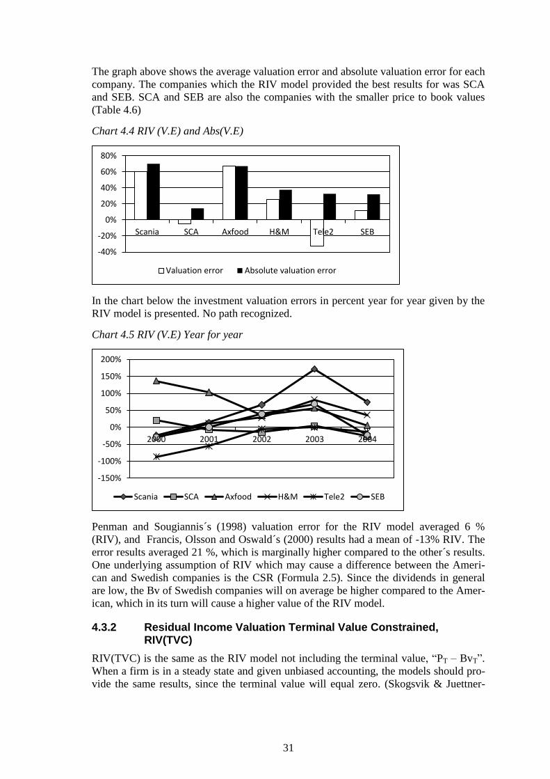
31

The graph above shows the average valuation error and absolute valuation error for each

company. The companies which the RIV model provided the best results for was SCA

and SEB. SCA and SEB are also the companies with the smaller price to book values

(Table 4.6)

Chart 4.4 RIV (V.E) and Abs(V.E)

In the chart below the investment valuation errors in percent year for year given by the

RIV model is presented. No path recognized.

Chart 4.5 RIV (V.E) Year for year

Penman and Sougiannis´s (1998) valuation error for the RIV model averaged 6 %

(RIV), and Francis, Olsson and Oswald´s (2000) results had a mean of -13% RIV. The

error results averaged 21 %, which is marginally higher compared to the other´s results.

One underlying assumption of RIV which may cause a difference between the Ameri-

can and Swedish companies is the CSR (Formula 2.5). Since the dividends in general

are low, the Bv of Swedish companies will on average be higher compared to the Amer-

ican, which in its turn will cause a higher value of the RIV model.

4.3.2 Residual Income Valuation Terminal Value Constrained, RIV(TVC)

RIV(TVC) is the same as the RIV model not including the terminal value, “PT – BvT”.

When a firm is in a steady state and given unbiased accounting, the models should pro-

vide the same results, since the terminal value will equal zero. (Skogsvik & Juettner-

-40%

-20%

0%

20%

40%

60%

80%

Scania SCA Axfood H&M Tele2 SEB

Valuation error Absolute valuation error

-150%

-100%

-50%

0%

50%

100%

150%

200%

2000 2001 2002 2003 2004

Scania SCA Axfood H&M Tele2 SEB

32

Nauroth, 2009) Based on the average absolute valuation error the model is ranked 3rd

,

and last when it comes to valuation error.

Table 4.10 RIV(TVC) (V.E) and Abs(V.E)

The companies which RIV(TVC) provided the best results for was SCA and Scania. As

stated above, these are the companies with the smallest price to book values.

Chart 4.6 RIV(TVC) (V.E) and Abs(V.E)

The undervaluation is clearly shown in the table. One reason for the consistent under-

valuation is due to the fact that the terminal value is not included and the Bv is not equal

to the price of the share at time T (after five years in this empirical study). Thereby, val-

uation bias is created since the companies on average have goodwill not taken into ac-

count in the formula.

Chart 4.7 RIV(TVC) (V.E) year for year

RIV(TVC) V.E 95% C.I. Abs.(V.E) 95% C.I.

Mean Std. Error Lower Upper Rank(V.E) Mean Std. Error Lower Upper Rank Abs(V.E.)

Scania -29,23% 0,186 -52,36% -6,09% 2 29,23% 0,186 6,09% 52,36% 2

SCA -16,89% 0,111 -30,65% -3,12% 1 16,89% 0,111 3,12% 30,65% 1

Axfood -42,68% 0,129 -58,67% -26,68% 3 42,68% 0,129 26,68% 58,67% 3

H&M -73,31% 0,092 -84,72% -61,90% 6 73,31% 0,092 61,90% 84,72% 6

Tele2 -51,81% 0,282 -86,83% -16,80% 5 51,81% 0,282 16,80% 86,83% 5

SEB -51,63% 0,111 -65,45% -37,82% 4 51,63% 0,111 37,82% 65,45% 4

Total -44,26% 0,237 -53,09% -35,43% 44,26% 0,237 35,43% 53,09%

-100%

-50%

0%

50%

100%

Scania SCA Axfood H&M Tele2 SEB

Valuation error Absolute valuation error

-120%

-100%

-80%

-60%

-40%

-20%

0%

2000 2001 2002 2003 2004

Scania SCA Axfood H&M Tele2 SEB

33

4.3.3 Abnormal Earning Growth, AEG

A large amount of the model´s value comes from the earnings per share, while the book

value only affects the value indirectly via the CSR. The underlying idea behind the

AEG model is that the equity value is built upon how much the firm earns, and should

therefore represent the share value. (Skogsvik & Juettner-Nauroth, 2009)

Table 4.11 AEG(V.E) and Abs(V.E)

AEG model performs on average an overestimation of 0,54 % of the value of the firm.

Even if the average valuation error was small, the absolute valuation error is as large as

49,03 %.Only FCFF and AEG(TVC) valuation model provided larger absolute valua-

tion error. The dispersion around the mean was also the second largest of all investment

models.

Chart 4.8 AEG (V.E) and Abs(V.E)

The smallest valuation bias and hence absolute valuation error are given to SCA, H&M

and SEB. SCA and SEB have the lowest and third lowest price to earnings ratio (Table

4.6). Both H&M and SEB has had a strong increase in the earnings per share for the

valued years, while SCA´s earnings has not grown to the same extent, but keeping a

stable level which seems to be preferable for the model. Due to the stability in the earn-

ings, SCA´s result is low with a small dispersion around the mean. Both Axfood and

Tele2 have had negative earnings for one versus two years during the investment valua-

tion period. This number was set to zero, but this affects the results and intervene the

preciseness of the model.

Chart 4.9 AEG (V.E) year for year

AEG V.E 95% C.I. Abs.(V.E) 95% C.I.

Mean Std. Error Lower Upper Rank(V.E) Mean Std. Error Lower Upper Rank Abs(V.E.)

Scania 45,87% 0,736 -45,54% 137,29% 5 61,97% 0,570 -8,81% 132,76% 5

SCA 0,94% 0,152 -17,89% 19,78% 1 11,20% 0,086 0,50% 21,91% 1

Axfood -51,29% 1,206 -201,02% 98,44% 6 111,89% 0,467 53,92% 169,87% 6

H&M 17,01% 0,434 -36,89% 70,92% 2 34,67% 0,273 0,80% 68,54% 2

Tele2 -39,64% 0,209 -65,61% -13,68% 4 39,64% 0,209 13,68% 65,61% 4

SEB 30,33% 0,448 -25,26% 85,93% 3 34,78% 0,405 -15,55% 85,11% 3

Total 0,54% 0,531 -65,37% 66,45% 49,03% 0,335 7,42% 90,63%

-60%

-40%

-20%

0%

20%

40%

60%

80%

100%

120%

140%

Scania SCA Axfood H&M Tele2 SEB

Valuation error Absolute valuation error

34

Axfood is the company with the highest variation from year to year, mostly due to both

negative and positive earnings. Both Axfood and Tele2´s negative earnings generate an

undervaluation and Axfood and Tele2. These companies are also the only two compa-

nies undervalued on average.

4.3.4 Abnormal Earning Growth Terminal Value Constrained, AEG(TVC)

The AEG(TVC) models are based on the AEG model, excluding the terminal value cal-

culation. In a similar manner to the RIV model, the AEG(TVC) assumes unbiased ac-

counting and that the company is acting in a steady state. Thereby the expression “PT +

DivT – XT * RE /rE“ is assumed to be zero. If this is not true, the model will provide val-

uation error. (Skogsvik & Juettner-Nauroth, 2009)

The valuation error and absolute valuation error are summarized below.

Table 4.12 AEG(TVC) (V.E) and Abs(V.E)

The empirical research shows both over- and undervaluation exists for the companies

using this method. On average, the model performed a 1,54% overestimation of value,

and an absolute valuation error on 49,54%. The average absolute valuation error was the

second largest out of the six models.

Chart 4.10 AEG(TVC) (V.E) and Abs(V.E)

-200%

-150%

-100%

-50%

0%

50%

100%

150%

200%

2000 2001 2002 2003 2004

Scania SCA Axfood H&M Tele2 SEB

AEG(TVC) V.E 95% C.I. Abs.(V.E) 95% C.I.

Mean Std. Error Lower Upper Rank(V.E) Mean Std. Error Lower Upper Rank Abs(V.E.)

Scania 52,43% 0,593 -21,23% 126,09% 4 61,17% 0,477 1,89% 120,45% 5

SCA 7,42% 0,586 -65,34% 80,18% 1 43,95% 0,330 2,99% 84,91% 3

Axfood 58,37% 0,427 5,41% 111,33% 5 58,37% 0,427 5,41% 111,33% 4

H&M -16,16% 0,334 -57,67% 25,34% 3 29,80% 0,183 7,11% 52,49% 2

Tele2 -81,64% 0,283 -116,82% -46,45% 6 81,64% 0,283 46,45% 116,82% 6

SEB -11,19% 0,261 -43,62% 21,25% 2 22,29% 0,148 3,97% 40,61% 1

Total 1,54% 0,621 -21,64% 24,72% 49,54% 0,363 35,98% 63,09%

35

The model performed the best valuation on SEB, H&M and SCA, the same as the AEG

model. The largest valuation is found when evaluating Tele2. As told above, this mod-

el´s benchmark is capitalized earnings. Tele2 has not had a consistent flow of income

during the investment years, leading to difficulties using this model. Negative earnings

are another part affecting the outcome.

Chart 4.11 AEG(TVC) (V.E) year for year

The valuation error varies from year to year and no specific path is found.

4.4 Free Cash Flow to the Firm, FCFF

As stated above, FCFF bases the investment valuation on the potential dividend.

Table 4.13 FCFF (V.E) and Abs(V.E)

-100%

-80%

-60%

-40%

-20%

0%

20%

40%

60%

80%

100%

Scania SCA Axfood H&M Tele2 SEB

Valuation error Absolute valuation error

-150%

-100%

-50%

0%

50%

100%

150%

2000 2001 2002 2003 2004

Scania SCA Axfood H&M Tele2 SEB

FCFF V.E 95% C.I. Abs.(V.E) 95% C.I.

Mean Std. Error Lower Upper Rank(V.E) Mean Std. Error Lower Upper Rank Abs(V.E.)

Scania 89,56% 0,724 -0,31% 179,44% 4 101,22% 0,496 39,65% 162,79% 4

SCA 174,58% 0,487 114,06% 235,10% 6 174,58% 0,487 114,06% 235,10% 5

Axfood 60,03% 0,563 -9,90% 129,96% 3 60,03% 0,563 -9,90% 129,96% 3

H&M 5,02% 0,223 -22,72% 32,76% 1 18,76% 0,095 6,95% 30,58% 1

Tele2 -58,93% 0,267 -92,12% -25,74% 2 58,93% 0,267 25,74% 92,12% 2

SEB -169,04% 2,289 -453,22% 115,13% 5 207,91% 1,846 -21,26% 437,09% 6

Total 16,87% 1,462 -37,72% 71,46% 103,57% 1,028 65,18% 141,97%

36

The FCFF model performs an overestimation of 16, 87 % on average. The absolute val-

uation error is as high as 103, 57 %, indicating the fact that the model contribute with

the least similar results to the actual market price of the share. The model does also have

the highest standard deviation.

Chart 4.12 FCFF (V.E) and Abs(V.E)

The model provided the best results to H&M, Tele2 and Axfood.

Chart 4.13 FCFF (V.E) year for year

As one can note from the table, large valuation errors exist for most of the companies.

SEB´s valuation from year to year varies, while Tele2 is consistent undervalued. SEB´s

FCFF result can be somewhat biased, due to the fact that FCFF fall short when evaluat-

ing a financial company due to the fact that these types of companies do not fit into the

general frame since the proportion of debt compared to equity is much higher for finan-

cial companies.

Penman and Sougiannis (1998) average valuation error for the FCFF approach averaged

-76%, while Francis, Olsson and Oswald´s (2000) result averaged 18%. This research

average valuation error turned out to be an overvaluation of 17 %, not far from Francis,

Olsson and Oswald´s results. The benchmark used in this model, EBIT, may vary due to

different accounting standards in IFRS and GAAP creating the differences in the results.

-200%

-100%

0%

100%

200%

300%

Scania SCA Axfood H&M Tele2 SEB

Valuation error Absolute valuation error

-600%

-500%

-400%

-300%

-200%

-100%

0%

100%

200%

300%

2000 2001 2002 2003 2004

Scania SCA Axfood H&M Tele2 SEB

37

5 Analysis and hypotheses testing

_____________________________________________________________________________

In this chapter a complete analysis is undertaken of the hypotheses and the investment models

connected to the theory described in section 2. Detailed answers to the stated questions found in

the hypotheses section are provided.

5.1 Testing hypotheses 1-6

Hypotheses 1-6 investigated if there were a significant difference between the mean of

the results provided by the investment models and the mean of the market prices. The

null hypothesis, HO, claims no significant difference exists between the means of the in-

vestment valuation model´s results and the market prices, while the alternative hypothe-

sis, HA, states that a significant difference exist. The tests were performed on the 1 %, 5

% and 10 % level of significance. The critical t-value for the empirical research is 2,76

for the 1% significance level, 2,05 for the 5% significance level and 1,70 for the 10 %

significance level.

If the hypothesis is accepted, no significant difference exists between the between the

results provided by the investment model and the market prices, while if the hypothesis

is rejected a significant difference exists.

Table 5.1 Results from the t-test

The result shows all investment models except the RIV(TVC) on the 1% and 5 % level

of significance accepted the null hypotheses and thereby no significant difference exists

between the results of the models and the market prices. On the significance level of 10

%, the PVED model was also rejected. What cannot be ignored is the fact that this test

is based on the means of both the market prices and the investment model´s results. If a

model is constantly over- or undervaluing, no fair result is attained since the mean

achieved by the investment model´s results will be higher or lower than the mean of the

market prices. This is the case for the RIV(TVC) model, the only investment model

constantly undervaluing all companies.

Result 1: All investment models’ results except RIV(TVC) provides no significant dif-

ference from the means of the market prices on 1 % and 5 % significance level.

5.2 Testing hypothesis 7

As recognized above, FCFF claims the value of the firm is represented by the potential

dividends while PVED states the actual dividends. As Swedish companies tend to have

a dividend policy which contains low dividend payouts and more reinvestment, the dif-

ference between the actual versus the potential dividends contribute to an interesting ex-

amination.

Diff FCFF-PVED= Abs(V.E)FCFF – Abs(V.E)PVED

Paired t-test of the means

Mean Val. model Mean Market value p-value t-value Sign. level 10% Sign. level 5% Sign. level 1%

PVED 70,35 86,43 0,06 1,95 Reject Ho Accept Ho Accept Ho

RIV 96,65 86,43 0,26 -1,14 Accept Ho Accept Ho Accept Ho

RIV(TVC) 44,11 86,43 0,00 6,14 Reject Ho Reject Ho Reject Ho

AEG 71,33 86,43 0,12 1,59 Accept Ho Accept Ho Accept Ho

AEG(TVC) 82,37 86,43 0,69 0,41 Accept Ho Accept Ho Accept Ho

FCFF 100,91 86,43 0,42 -0,82 Accept Ho Accept Ho Accept Ho

38

If the mean difference tested in the t-test is significant negative (positive) mean values

implies that the absolute valuation error for FCFF on average is smaller (greater) than

the valuation error in PVED. The null hypothesis states no difference exists between the

models´ valuation errors.

Table 5.2 T-test FCFF and PVED

The mean represents the mean difference between the absolute valuation errors. A sig-

nificant difference exists, and FCFF tends to provide higher valuation errors compared

to PVED. Thereby the value of equity tend on average be better represented by the actu-

al dividend than the potential dividend.

Chart 5.1 Abs(V.E) for PVED and FCFF

PVED provide on average smaller absolute valuation for four out of six companies

(Scania, SCA, Axfood and SEB). The largest difference between the two models can be

found when evaluating SEB. SEB pays out dividends around 40% of earnings, which

tends to better reflect the market price than the potential dividend. The large gap ob-

served is also partly due to the fact that the FCFF model does not provide fair results

when the level of debt compared to the level of equity in the balance sheet is high

(which it is in SEB:s case, due to the company´s financial nature).

The smallest valuation error difference between the FCFF and PVED model was found

when evaluating H&M and Axfood. Axfood´s dividend policy includes paying out at

least 50% of the profit after tax and H&M dividends also equal around half amount of

the profit after tax. Hence, the higher actual dividends, the closer to potential dividends

which will make the FCFF and PVED results more similar. Tele2 has no specific divi-

dend policy. SCA has stable and rising dividends, approximately 1/3 of the cash flow

after interest and tax. Scania focuses on long term value rather than fixed dividend poli-

cy.

The difference between the valuation results for all observations can be observed below.

Chart 5.2 Abs(V.E)FCFF – Abs(V.E)PVED

Paired t-test of the means Mean P-value t-value Sign. level 10% Sign. level 5% Sign. level 1%

Total 69,51% 0,00222 3,36 Reject Ho Reject Ho Reject Ho

0%

50%

100%

150%

200%

250%

Scania SCA Axfood H&M Tele2 SEB

PVED FCFF

39

The expression Abs(V.E)FCFF – Abs(V.E)PVED is mostly positive, which means in gen-

eral Abs(V.E)FCFF is larger than Abs(V.E)PVED.

Result 2: The PVED provide on average smaller absolute valuation errors compared to

FCFF, for four out of six companies (Scania, SCA, Axfood and SEB).

5.3 Testing hypotheses 8 - 11

As stated above, in previous studies investigated American companies by Pennman and

Sougiannis (1998) and Francis, Olsson and Oswald (2000), results show that the RIV

method (and hence earnings methods) dominate the cash flow and the dividend tech-

niques. These results will be investigated further in order to find out if this is the same

for the empirical results in this paper considering Swedish companies. In hypotheses 8

and 9 RIV and RIV(TVC) absolute valuation errors are explored and compared to both

PVED and FCFF models. Hypotheses 10 and 11 include the same procedure for AEG

and AEG(TVC) models.

5.3.1 Residual Income Valuation, RIV

The RIV model was first compared to PVED model.

Diff PVED-RIV= Abs(V.E)PVED – Abs(V.E)RIV

Table 5.3 Paired t-test PVED and RIV

PVED provides smaller absolute evaluation error, compared to RIV model, but no sig-

nificant difference exists.

The chart below emphasizes the absolute valuation errors for all the companies, stated

as a mean for all investigated investment years.

Chart 5.3 Abs(V.E) PVED and RIV

-200%

0%

200%

400%

600%

0 5 10 15 20 25 30 35

Abs(V.E)FCFF-Abs(V.E)PVED

Paired t-test of the means Mean P-value t-value Sign. level 10% Sign. level 5% Sign. level 1%

Total -8,25% 0,309 -1,04 Accept Ho Accept Ho Accept Ho

40

The absolute valuation error is mostly similar on SCA, Axfood and H&M.

The chart below shows all 30 investment valuation results difference in valuation error.

Chart 5.4 Abs(V.E)PVED – Abs(V.E)RIV

On average it is 8,25 % negative, and thereby larger valuation errors are on average

provided by RIV.

The next t-test is exploring the difference between RIV and FCFF.

Diff FCFF-RIV= Abs(V.E)FCFF – Abs(V.E)RIV

Table 5.4 Paired t-test FCFF and RIV

A major difference exists between the valuation errors, and RIV errors are smaller and

hence preferable. The hypothesis is rejected on all levels.

Chart 5.5 Abs(V.E) FCFF and RIV

0%

10%

20%

30%

40%

50%

60%

70%

80%

Scania SCA Axfood H&M Tele2 SEB

PVED RIV

-200%

-150%

-100%

-50%

0%

50%

100%

0 5 10 15 20 25 30 35

Abs(V.E)PVED-Abs(V.E)RIV

Paired t-test of the means Mean P-value t-value Sign. level 10% Sign. level 5% Sign. level 1%

Total 61,27% 0,00442 3,09 Reject Ho Reject Ho Reject Ho

41

The companies with the smallest difference between the absolute valuation errors are

Axfood and H&M, while SEB and SCA have the largest difference.

All difference in the valuation errors can be observed below.

Chart 5.6 Abs(V.E)FCFF – Abs(V.E)RIV

The valuation error spreads are on average providing a positive difference, emphasizing

the smaller valuation bias for the RIV model.

5.3.2 Residual Income Valuation Terminal Value Constrained, RIV(TVC)

The difference between the valuation errors are compared for the RIV(TVC) and the

PVED model.

Diff PVED-RIV(TVC)= Abs(V.E)PVED – Abs(V.E)RIV(TVC)

Table 5.5 Paired t-test PVED and RIV(TVC)

0%

50%

100%

150%

200%

250%

Scania SCA Axfood H&M Tele2 SEB

FCFF RIV

-100%

0%

100%

200%

300%

400%

500%

600%

0 5 10 15 20 25 30 35

Abs(V.E)FCFF-Abs(V.E)RIV

Paired t-test of the means Mean P-value t-value Sign. level 10% Sign. level 5% Sign. level 1%

Total -10,20% 0,202 -1,31 Accept Ho Accept Ho Accept Ho

42

The result indicates the recognition of the higher valuation errors provided by

RIV(TVC), but not significantly large since the t-test is not rejected on the three various

levels. On average the difference is - 10,2 % in the absolute valuation error.

The companies´ absolute valuation errors are summarized below.

Chart 5.7 Abs(V.E) PVED and RIV(TVC)

PVED provided smaller valuation errors for Scania, H&M and SEB. The largest differ-

ences exist when valuating H&M and SEB.

The chart below all observation differences can be observed.

Chart 5.8 Abs(V.E)PVED – Abs(V.E)RIV(TVC)

The results are mostly negative, emphasizing the superiority of the PVED model.

The valuation errors between RIV(TVC) and FCFF are also compared.

Diff FCFF-RIV(TVC)= Abs(V.E)FCFF – Abs(V.E)RIV(TVC)

Table 5.6 Paired t-test FCFF and RIV(TVC)

0%

10%

20%

30%

40%

50%

60%

70%

80%

Scania SCA Axfood H&M Tele2 SEB

PVED RIV(TVC)

-100%

-50%

0%

50%

100%

150%

0 5 10 15 20 25 30 35

Abs(V.E)PVED-Abs(V.E)RIV(TVC)

Paired t-test of the means Mean P-value t-value Sign. level 10% Sign. level 5% Sign. level 1%

Total 59,32% 0,00686 2,91 Reject Ho Reject Ho Reject Ho

43

FCFF provides larger valuation errors, and significant valuation errors between the

models exist on all levels and the null hypothesis is rejected.

FCFF and RIV(TVC) valuation errors for the companies are summarized in the chart

below.

Chart 5.9 Abs(V.E) FCFF and RIV(TVC)

RIV(TVC) provided smaller errors for all companies except H&M. The largest valua-

tion errors are found when valuating SCA and SEB (the same as when RIV and FCFF

models are compared).

The difference between the valuations errors are shown in the chart below.

Chart 5.10 Abs(V.E)FCFF – Abs(V.E)RIV(TVC

The difference tends to be positive, indicating higher errors for the FCFF model.

5.3.3 Abnormal Earning Growth, AEG

The PVED model is compared with the AEG model.

Diff PVED-AEG= Abs(V.E)PVED – Abs(V.E)AEG

Table 5.7 Paired t-test PVED and AEG

0%

50%

100%

150%

200%

250%

Scania SCA Axfood H&M Tele2 SEB

FCFF RIV(TVC)

-100%

0%

100%

200%

300%

400%

500%

0 5 10 15 20 25 30 35

Abs(V.E)FCFF-Abs(V.E)RIV(TVC)

Paired t-test of the means Mean P-value t-value Sign. level 10% Sign. level 5% Sign. level 1%

Total -14,96% 0,0888 -1,76 Reject Ho Accept Ho Accept Ho

44

When comparing PVED and AEG approach, the results show smaller valuation errors

for PVED with a mean of 14,96%, but at the 1 % and 5 % significance level no signifi-

cant difference between the means of the valuation errors existed. The null hypothesis is

rejected at the 10 % level.

The companies´ absolute valuation errors for PVED and AEG are summarized below.

Chart 5.11 Abs(V.E) PVED and AEG

The largest difference in valuation errors can be found when evaluating Axfood and

Scania. PVED provides smaller average evaluation error on all companies except for

Tele2 and SCA.

All observed differences in errors are summarized in the table below.

Chart 5.12 Abs(V.E)PVED – Abs(V.E)AEG

Mostly negative differences for the valuation errors can be observed in the chart.

FCFF and AEG were also compared.

Diff FCFF-AEG= Abs(V.E)FCFF – Abs(V.E)AEG

Table 5.8 Paired t-test FCFF and AEG

0%

20%

40%

60%

80%

100%

120%

Scania SCA Axfood H&M Tele2 SEB

PVED AEG

-200%

-150%

-100%

-50%

0%

50%

100%

0 5 10 15 20 25 30 35

Abs(V.E)PVED-Abs(V.E)AEG

Paired t-test of the means Mean P-value t-value Sign. level 10% Sign. level 5% Sign. level 1%

Total 54,55% 0,0165 2,55 Reject Ho Reject Ho Accept Ho

45

The valuation errors for FCFF were larger. Significant difference exists between the

valuation errors between the models on 5 % and 10 % level. The difference in the valu-

ation errors for FCFF and AEG models is on average 54,55 % larger for the FCFF.

The absolute valuation errors for all companies are summarized below.

Chart 5.13 Abs(V.E) FCFF and AEG

FCFF provided much larger errors for SCA and SEB. Scania´s FCFF error was also

larger. For H&M and Axfood AEG model performed larger valuation errors.

All observations’ valuation error differences are summarized in the chart below.

Chart 5.14 Abs(V.E)FCFF – Abs(V.E)AEG

The differences tend on average to be positive, claiming superiority of the AEG model.

5.3.4 Abnormal Earning Growth Terminal Value Constrained, AEG(TVC)

AEG(TVC) and PVED absolute valuation errors were also examined.

Diff PVED-AEG(TVC)= Abs(V.E)PVED – Abs(V.E)AEG(TVC)

Table 5.9 Paired t-test PVED and AEG(TVC)

0%

50%

100%

150%

200%

250%

Scania SCA Axfood H&M Tele2 SEB

FCFF AEG

-200%

0%

200%

400%

600%

0 5 10 15 20 25 30 35

Abs(V.E)FCFF-Abs(V.E)AEG

Paired t-test of the means Mean P-value t-value Sign. level 10% Sign. level 5% Sign. level 1%

Total -15,47% 0,0195 -2,47 Reject Ho Reject Ho Accept Ho

46

PVED provided smaller valuation errors than AEG(TVC), and the null hypothesis is ac-

cepted on the 1 % level of significance, but rejected on the 5 % and 10 % level.

All the observations´ difference in valuation error can be observed in the diagram be-

low.

Chart 5.15 Abs(V.E) PVED and AEG(TVC)

The differences are on average negative by -15, 47 %, indicating that the AEG(TVC)

model on average provides higher valuation error.

The chart below summarizes the absolute valuation errors for the companies.

Chart 5.16 Abs(V.E)PVED – Abs(V.E)AEG(TVC)

PVED provides smaller valuation errors for all the companies. The least difference be-

tween the valuation errors existed when evaluating Axfood.

The FCFF model´s valuation errors are also examined in relation to the AEG(TVC) val-

uation errors.

Diff FCFF-AEG(TVC)= Abs(V.E)FCFF – Abs(V.E)AEG(TVC)

Table 5.10 Paired t-test FCFF and AEG(TVC)

-150%

-100%

-50%

0%

50%

100%

0 5 10 15 20 25 30 35

Abs(V.E)PVED-Abs(V.E)AEG(TVC)

0%

10%

20%

30%

40%

50%

60%

70%

80%

90%

Scania SCA Axfood H&M Tele2 SEB

PVED AEG(TVC)

47

Even if AEG(TVC) produces larger valuation error than PVED, the FCFF´s valuation

errors are larger compared to AEG(TVC). A significant difference exists between the

valuation errors and the null hypothesis is rejected on all significance levels. Hence, a

significant difference exists between the results provided by FCFF model and the

AEG(TVC) model, in favor of the AEG(TVC) model.

The absolute valuation error for each company is summarized below.

Chart 5.17 Abs(V.E) FCFF and AEG(TVC)

H&M and Tele2 were the only two firms which FCFF investment model provided better

results for. Large valuation error differences exist when evaluating SCA and SEB.

All the observations´ differences of valuation error can be observed below.

Chart 5.18 Abs(V.E)FCFF – Abs(V.E)AEG(TVC)

Paired t-test of the means Mean P-value t-value Sign. level 10% Sign. level 5% Sign. level 1%

Total 54,04% 0,00863 2,82 Reject Ho Reject Ho Reject Ho

0,00%

50,00%

100,00%

150,00%

200,00%

250,00%

Scania SCA Axfood H&M Tele2 SEB

FCFF AEG(TVC)

-200,00%

-100,00%

0,00%

100,00%

200,00%

300,00%

400,00%

500,00%

600,00%

0 5 10 15 20 25 30 35

Abs(V.E)FCFF-Abs(V.E)AEG(TVC)

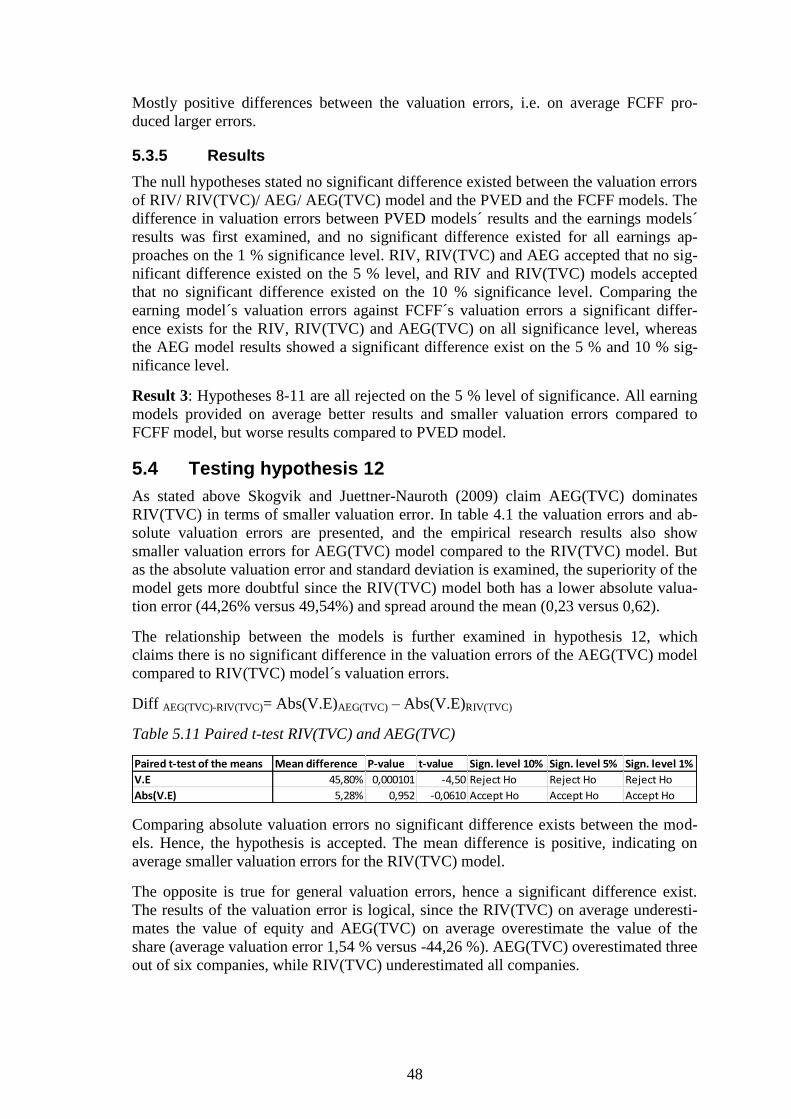
48

Mostly positive differences between the valuation errors, i.e. on average FCFF pro-

duced larger errors.

5.3.5 Results

The null hypotheses stated no significant difference existed between the valuation errors

of RIV/ RIV(TVC)/ AEG/ AEG(TVC) model and the PVED and the FCFF models. The

difference in valuation errors between PVED models´ results and the earnings models´

results was first examined, and no significant difference existed for all earnings ap-

proaches on the 1 % significance level. RIV, RIV(TVC) and AEG accepted that no sig-

nificant difference existed on the 5 % level, and RIV and RIV(TVC) models accepted

that no significant difference existed on the 10 % significance level. Comparing the

earning model´s valuation errors against FCFF´s valuation errors a significant differ-

ence exists for the RIV, RIV(TVC) and AEG(TVC) on all significance level, whereas

the AEG model results showed a significant difference exist on the 5 % and 10 % sig-

nificance level.

Result 3: Hypotheses 8-11 are all rejected on the 5 % level of significance. All earning

models provided on average better results and smaller valuation errors compared to

FCFF model, but worse results compared to PVED model.

5.4 Testing hypothesis 12

As stated above Skogvik and Juettner-Nauroth (2009) claim AEG(TVC) dominates

RIV(TVC) in terms of smaller valuation error. In table 4.1 the valuation errors and ab-

solute valuation errors are presented, and the empirical research results also show

smaller valuation errors for AEG(TVC) model compared to the RIV(TVC) model. But

as the absolute valuation error and standard deviation is examined, the superiority of the

model gets more doubtful since the RIV(TVC) model both has a lower absolute valua-

tion error (44,26% versus 49,54%) and spread around the mean (0,23 versus 0,62).

The relationship between the models is further examined in hypothesis 12, which

claims there is no significant difference in the valuation errors of the AEG(TVC) model

compared to RIV(TVC) model´s valuation errors.

Diff AEG(TVC)-RIV(TVC)= Abs(V.E)AEG(TVC) – Abs(V.E)RIV(TVC)

Table 5.11 Paired t-test RIV(TVC) and AEG(TVC)

Comparing absolute valuation errors no significant difference exists between the mod-

els. Hence, the hypothesis is accepted. The mean difference is positive, indicating on

average smaller valuation errors for the RIV(TVC) model.

The opposite is true for general valuation errors, hence a significant difference exist.

The results of the valuation error is logical, since the RIV(TVC) on average underesti-

mates the value of equity and AEG(TVC) on average overestimate the value of the

share (average valuation error 1,54 % versus -44,26 %). AEG(TVC) overestimated three

out of six companies, while RIV(TVC) underestimated all companies.

Paired t-test of the means Mean difference P-value t-value Sign. level 10% Sign. level 5% Sign. level 1%

V.E 45,80% 0,000101 -4,50 Reject Ho Reject Ho Reject Ho

Abs(V.E) 5,28% 0,952 -0,0610 Accept Ho Accept Ho Accept Ho

49

Result 4: The paired t-test shows no significant difference exist between the means of

AEG(TVC) and RIV(TVC) absolute valuation errors. RIV(TVC) provides on average

smaller absolute valuation errors, thereby creating smaller valuation bias, even if not

significant. A significant difference exists when valuation errors are compared. The dif-

ference is created since the result provided by AEG(TVC) model is on average to high,

while RIV(TVC) provides to low estimation.

5.5 Testing hypotheses 13 & 14

As mentioned above both the RIV and the AEG models have a constrained and an un-

constrained version. If the firm is in steady state there should be no need for including

the terminal value, since it should equal zero. In hypotheses 13 & 14 the valuation er-

rors results will be examined to find out whether including or not including the terminal

value calculation provides a significant difference in the valuation errors.

Diff AEG-AEG(TVC)= Abs(V.E)AEG – Abs(V.E)AEG(TVC)

Diff RIV-RIV(TVC)= Abs(V.E)RIV – Abs(V.E)RIV(TVC)

Table 5.12 Paired t-tests RIV and RIV(TVC) , AEG and AEG(TVC)

When testing the various approaches in paired t-test, neither of the approaches´ versions

provide significant differences between the valuation errors, so neither null hypothesis

can be neglected. The inclusion of the terminal value does not provide a significant dif-

ference, even though it contributes to smaller valuation bias on average since the con-

servative accounting is taken into account.

Result 5: Neither the constrained nor the unconstrained versions of the RIV or AEG

approaches provide a significant difference in the size of the valuation errors. On aver-

age, the unconstrained versions of RIV and AEG provide smaller absolute valuation er-

rors, which mean that on average including the terminal value paid off. Hence, on aver-

age companies are not acting in a steady state and goodwill/badwill exists produced by

conservative accounting.

5.6 Fundamentals of companies

The expectations, as well as company information, tend to have influence on the stock

price. By investigating the fundamentals of a company and comparing it to the various

model´s valuation errors my purpose was to see if any connections to the valuation

model´s result could be found.

The table below shows the ranking of which model provided the smallest absolute valu-

ation results for each company.

Table 5.13 Ranking of Abs(V.E)

Paired t-test of the means Mean difference P-value t-value Sign. level 10%Sign. level 5%Sign. level 1%

RIV, RIV(TVC) -1,95% 0,833 -0,213 Accept Ho Accept Ho Accept Ho

AEG, AEG(TVC) -0,51% 0,952 -0,0610 Accept Ho Accept Ho Accept Ho

50

In table 4.2 and 4.3 all the companies´ valuation errors and absolute valuation errors are

summarized. The investment method which provided the least absolute valuation error

for Scania was PVED, for SCA AEG, for Axfood RIV(TVC), for H&M FCFF, for

Tele2 RIV and for SEB PVED. Table 4.3 and 5.13 emphasizes the superiority of the

PVED and the high level of valuation bias for the FCFF model. FCFF is the model with

the highest level of valuation bias for three companies, hence 50 %.

Table 5.14 Investment models result information

Overview of results from the empirical results, (+) represents positive average valuation

error and (-) negative average valuation error.

The average absolute valuation error for all investment methods was smallest on H&M,

followed by SCA, Scania, SEB, Tele2 and Axfood (table 4.3). An underestimation was

on average done on H&M, Tele2 and SEB, while Scania, SCA and Axfood were over-

valued on average. The investment valuation methods perform the best on companies

listed for the longest number of years. On average, the highest valuation error arises

when valuating Tele2, the company listed on the stock exchange the shortest amount of

time.

SCA is the company with the average highest earnings, followed by H&M, Scania,

SEB, Tele2 and Axfood. Switching H&M´s and SCAs positions creates exactly the

same order as the average absolute error. Hence, the larger earnings the less absolute

valuation errors.

Result 6: On average, companies with larger earnings and longer listed on the exchange

leading to less valuation bias.

Company PVED RIV RIV(TVC) AEG AEG(TVC) FCFF

Scania 1 5 2 4 3 6

SCA 4 2 3 1 5 6

Axfood 2 5 1 6 3 4

H&M 2 5 6 4 3 1

Tele2 5 1 2 4 6 3

SEB 1 3 5 4 2 6

Mean 2,5 3,5 3,167 3,833 3,667 4,333

Average V.E. Average absolute V.E.

over-/underestimation largest error Smallest error Largest error Smallest error

PVED Underest. 5/6 companies Tele2(-), Axfood (+) SEB (-), SCA(-) Tele2, Axfood SEB, SCA

RIV Overest. 4/6 companies Scania (+) Axfood (+) SCA (-), SEB (+) Scania, Axfood SCA,SEB

RIV(TVC) Under all companies H&M (-), tele2 (-) SCA (-), Scania (-) H&M, Tele2 SCA, Scania

AEG Underest. 2/6 companies Tele2 (-), Axfood (-) SCA (+), H&M (+) Axfood, Tele2 SCA, H&M

AEG(TVC) Over 3/6 companies Tele2(-), Axfood (+) SCA (+), SEB (-) Tele2, Scania SEB, H&M

FCFF Over 4 /6 companies SCA (+), SEB(-) H&M (+), Tele2 (-) SEB, SCA H&M, Tele2

51

6 Discussion of empirical results

_____________________________________________________________________________ Below the hypotheses and the results are summarized. Further the results are discussed in

more detail.

6.1 Hypotheses and results

In order to provide an overview, the hypotheses and the results are summarized in the

table below.

Table 6.1 Summarization of hypotheses and results

Null Hypothesis Result

1. No significant difference between the

mean of the results of the PVED model

and the market prices exist.

Accept the null hypothesis on 1 % and 5

% significance level.

2. No significant difference between the

mean of the results of the RIV model and

the market prices exist.

Accept null hypothesis for all significance

levels.

3. No significant difference between the

mean of the results of the RIV(TVC)

model and the market prices exist.

Reject null hypothesis for all significance

levels.

4. No significant difference between the

mean of the results of the AEG model and

the market prices exist.

Accept null hypothesis for all significance

levels.

5. No significant difference between the

mean of the results of the AEG(TVC)

model and the market prices exist.

Accept null hypothesis for all significance

levels.

6. No significant difference between the

mean of the results of the FCFF model

and the market prices exist.

Accept null hypothesis on all significance

levels.

7. No significant difference between the

mean of the absolute valuation results of

the FCFF model and the PVED model.

Reject null hypothesis on all significance

levels. PVED model provides significant

smaller absolute valuation errors.

8. RIV on average provides no significant

difference in the absolute valuation errors

results compared to both PVED and

FCFF.

Reject null hypothesis. The RIV model

provides on average no significant differ-

ence in absolute valuation errors com-

pared with the PVED model on all levels,

but compared with the FCFF model a sig-

nificant difference on all levels.

9. RIV(TVC) on average provides no sig-

nificant difference in absolute valuation

errors results compared to both PVED and

Reject null hypothesis. The RIV(TVC)

model provides on average no significant

difference in absolute valuation errors

52

FCFF. compared with the PVED model on all

levels, but compared with the FCFF mod-

el a significant difference on all levels.

10. AEG on average provides no signifi-

cant difference in absolute valuation er-

rors results compared to both PVED and

FCFF.

Reject null hypothesis. The AEG model

provides on average a significant differ-

ence in absolute valuation errors com-

pared with the PVED model on the 10 %

level, and compared with the FCFF model

a significant difference on the 5 % and 10

% level.

11. AEG(TVC) on average provides no

significant difference in absolute valuation

errors results compared to both PVED and

FCFF.

Reject null hypothesis. The AEG(TVC)

model provides on average a significant

difference in absolute valuation errors

compared with the PVED model on the 5

% and 10 % level, and compared to the

FCFF model a significant difference on all

levels.

12. AEG(TVC) provides no significant

difference in the absolute valuation errors

results compared to RIV(TVC).

Accept the null hypothesis for all signifi-

cance levels. Absolute valuation errors

provided by RIV(TVC) model are smaller,

but not significant different. The

AEG(TVC) model has a larger variation

than RIV(TVC) model.

13. RIV(TVC) provides no significant ab-

solute errors results compared to RIV.

Accept the null hypothesis on all signifi-

cance levels. The RIV model provides

smaller absolute valuation errors, but not

significant different.

14. AEG(TVC) provides no significant

absolute errors results compared to AEG.

Accept the null hypothesis on all signifi-

cance levels. The AEG model provides

smaller absolute valuation errors, but not

significant different.

Hypotheses 1-6 investigated if a significant difference exists between the mean of the

market prices and the mean of the investment model´s results. Accepting the null hy-

pothesis means that no significant gap exists between the mean of the investment mod-

el´s results and the mean of the market prices. For hypotheses 1-6 all hypotheses except

1 and 3 (including PVED and RIV(TVC) model) accepted the null hypotheses, thereby

claiming no significant difference exist on all the significance levels. Hence, the validity

is high for the RIV, AEG, AEG(TVC) and FCFF, since all the levels of significance

were accepted.

Hypothesis 1 investigated the difference between the market prices and the PVED mod-

el´s results. The hypothesis is rejected on the 10 % level. Hypothesis 3 examined

RIV(TVC) model´s results and the market prices, and rejects the null hypothesis on all

levels, and thereby a significant difference exists. The test is neglected for the

53

RIV(TVC) model due to the fact that the model provides underestimation for all the

companies, thereby creating a much smaller mean compared to the market prices´ mean.

The same is true for PVED, since the model undervalued five out of six companies.

When it comes to the absolute valuation error, RIV(TVC) contributes to the third small-

est while PVED has the smallest absolute valuation error. The RIV(TVC) model also

provided the smallest dispersion around the mean, and thereby has a high reliability.

The low level of variation makes the model attractive to use even if undervaluation is

achieved, since a small confidence interval is created. An investor can be 95% sure that

the model´s result will be -53,09% to -35.43% lower than the market price.

Both AEG and AEG(TVC) models´ t-test showed no results of neglecting hypotheses 3

and 4. The smallest average valuation error among all models was provided by AEG,

followed by AEG(TVC). Hence, this information claims the same results as Skogvik

and Juettner-Nauroth (2009) outcome. Even if small valuation errors are achieved, the

standard deviations for both models are large. The models provide almost the same

amount of over- and undervaluation of the companies [AEG overestimates two and

AEG(TVC) three out of six companies] and thereby the high and the low valuations

tend to cancel each other out, resulting in small means. Hence, basing the choice of a

single stock on AEG or AEG(TVC)’s results share is a risky choice, while a portfolio

composition may appear to be a better decision.

In hypothesis 6 FCFF model´s results are examined in relation to the market prices, and

no significant difference exists. In hypothesis 7 the FCFF model´s results are also in-

cluded, but the relationship between the FCFF and PVED models´ results are instead

compared. Hypothesis 7 is rejected, claiming a significant difference exists between the

investment models results, in favor of PVED.

On average, PVED model provided undervaluation while FCFF model generated over-

valuation. The signs of the valuation errors make sense since using potential dividend

(FCFF) is generally larger than the actual dividends (PVED). The higher actual divi-

dends the closer to potential dividends, creating the FCFF and the PVED models´ re-

sults more similar.

One reason for the PVED model´s superiority to the FCFF model is that management

easier can control the actual dividends than the potential dividends, contributing to less

variation for the PVED model. The PVED model´s variance is almost 3 times smaller

than the FCFF model´s (0,361 versus 1,028). Valuing a company with a stable dividend

policy is preferred when the PVED model is applied. This is due to the fact that a con-

sistent flow of value creates higher investment valuation results.

The only company the PVED model overestimated was Axfood, which does not strike

as surprising since the company has a dividend policy including the highest payout ratio

Axfood´s dividend policy is a promise to pay out at least 50% of the profit after tax,

while the other companies use approximations in the policy.

The best results and hence the smallest valuation error using the PVED model was pro-

vided when evaluating SEB, followed by SCA. SEB pay out dividends around 40% of

earnings, while SCA policy contains stable and rising dividends, and approximately 1/3

of the cash flow after interest and tax are paid out. Hence, the PVED model seems to

create the smallest valuation errors for those companies paying out little less than half

the amount of profits in dividends.

54

As told above, PVED generate undervaluation and FCFF undervaluation on average.

Hence, the actual dividends do not capture the whole market price, while potential divi-

dends characterize too much of the value. A mixed model of these valuation methods

would on average better fit the Swedish companies with its low paying dividends and

large reinvestment amounts. An alternative approach of the PVED model is the Present

Value of Expected Earnings (PVEE) model, in which the dividend payout ratio, k, is in-

cluded.

Formula 6.1 PVEE

T

V0PVEE

= ∑ E0(kt*Xt)/REt + E0((kT+1 * XT+1)/(rE

T+1-g))/RE

T

t=1

PVEE is an attractive model to use, since the model does not depend on the dividend

policies, while the major drawback is the fact that it is solely focusing on the future

earnings when calculating the value of owners´ equity.

By comparing the PVED results with the PVEE results gaps may be found. If large gaps

exist, the valuation results should be used with suspicion. The company´s dividend poli-

cy or the actual dividend might not represent a fair value of the firm´s equity and there-

by the PVEE and PVED model respectively do not provide reasonable results, and

thereby using other models may be preferred.

In hypotheses 8 – 11 all the earnings methods are compared to the PVED and the FCFF

model. All earnings methods are preferred over FCFF, and the underlying idea of the

FCFF model that cash flow represents the true value of the firm since accounting leads

to distortions (Penman & Sougiannis, 1998) is not supported by these results. The

PVED model was also preferred over the earnings methods, supporting the idea that

dividends are the payoff which represents the value of a company best.

As told above, the AEG(TVC) model provides on average smaller valuation errors

compared to RIV(TVC) model if the growth in the terminal period is small enough. The

valuation errors for the AEG(TVC) approach arise due to the capitalized growth of the

conservative bias in the terminal period while RIV(TVC) valuation errors are caused by

the magnitude of the conservative bias of owners´ equity value at the terminal point of

time. (Skogsvik & Juettner-Nauroth, 2009)

The terminal value constrained versions of AEG and RIV models are compared in hy-

pothesis 12. Skogvik and Juettner-Nauroth (2009) claim AEG(TVC) model dominates

RIV(TVC) model in terms of smaller valuation error. This supports the results from this

paper as well, since the AEG(TVC) method on average provides smaller valuation error

(1,54%, compared to -44,26%). Thereby, the growth in the terminal period is small

enough. But no significant difference exists in the paired t-test comparing the

RIV(TVC) and AEG(TVC) model. But as standard deviation (0,363 versus 0,237) and

absolute valuation error (49, 54% versus 44, 26%) for the RIV(TVC) and AEG(TVC)

models are considered, the superiority of the AEG(TVC) model gets doubtful. The

RIV(TVC) model has a greater ability to withstand the valuation bias since the absolute

valuation error is smaller, thereby making the model more robust to withstand valuation

bias.

As told above in section 4.4, book value and earnings calculated to perpetuity are the

benchmarks for the RIV and the AEG models respectively. Both these inputs provide

55

constant undervaluation for the companies over time, supporting the statement that a

premium exists and should be included in order to estimate a more fair value of equity.

When the residual income or abnormal earnings are added to the benchmarks, smaller

valuation bias is achieved. In hypothesis 13 and 14 the earnings formulas are further in-

vestigated in order to find out whether including the terminal calculation is worthwhile.

In hypothesis 13, RIV is compared to RIV(TVC). Even though the t-test results show no

significant difference exist between the valuation errors, the RIV provides both better

valuation error and absolute valuation error on average.

In hypothesis 14 AEG and AEG(TVC) models are compared. The null hypothesis

states no significant difference exists is not rejected, but the AEG model is on average

providing somewhat smaller valuation error and absolute valuation error (0,54 % and

49,08 % compared to 1,54 % and 49,54 %). A low price to earnings ratio leads in gen-

eral to better estimates using these models.

On one hand, RIV and AEG models are unaffected by conservative accounting. On the

other hand, RIV(TVC) and AEG(TVC) models are affected, creating a possible valua-

tion bias. Thereby, the difference between these models valuation errors are caused by

conservative accounting, and the RIV(TVC) model´s valuation error depends on the

conservative bias of the value of equity at the horizon time, while the valuation bias of

the AEG(TVC) model depends on the capitalized growth of the conservative bias in the

terminal period. The results show that the unconstrained versions provide smaller valua-

tion bias, and thereby one can conclude that conservative accounting is on average pre-

sent and generate valuation bias for the RIV(TVC) and AEG(TVC) models. Hence, on

average companies are not acting in a steady state and goodwill/badwill exists at the

chosen horizon of time, T.

6.2 Company information and valuation bias

The companies which on average were undervalued were H&M, Tele2 and SEB, while

Scania, SCA and Axfood were on average overvalued (Table 4.2). The high variance

provided by Axfood is mostly due to a high variance in the earnings, which have been

both negative and positive.

The smallest average absolute valuation error for the companies was given to H&M,

followed by SCA, Scania, SEB, Tele2 and Axfood (Table 4.3). The results indicate that

investment valuation results are on average more accurate for companies with larger

earnings and longer public listing. Hence, more stable firms tend to be easier to esti-

mate. New corporations have a tendency to have more expectations and less certain fu-

ture, which is often reflected in the share price. Expectations make investment valuation

problematic, and even more challenging for more complex models since ambiguous in-

puts needs to be estimated.

H&M turned out to be the company with the lowest level of valuation bias, and the

company is acting in a market with a high market share and many tangible assets

marked to market on the balance sheet. H&M tend to have high reliability in their re-

sults as well, since H&M has the lowest variance.

Tele2 is instead a company operating within information technology, an industry often

recognized with a high amount of intangible assets hidden on the balance sheet, thereby

creating difficulties when evaluating the company using investment models based on

56

numbers from the financial statements. Thereby, the average undervaluation of the

company does not strike surprising. The company has also been listed short amount of

time compared to the other companies, and thereby the fundamentals may not yet be

perfectly reflected in the market value. 5

6.3 Swedish versus American companies

Countries with civil laws, e.g. Sweden, pay on average fewer dividends compared to

countries using common law, e.g. USA (La Porta et al., 2000). Since the Swedish firms

are instead focusing on the reinvestment needs the financial statements look slightly dif-

ferent and thereby somewhat altered benchmark is created when evaluating Swedish

and American companies. The level of conservative accounting is another issue affect-

ing the financial statements in the countries. The somewhat different financial state-

ments is one reason why the results provided in this paper is to some extent inconsistent

with the results generated by Penman and Sougiannis (1998) and Francis, Olsson and

Oswald (2000), examining American firms. The results in this paper indicate a superior-

ity of the PVED model, while the two articles mentioned above favored the RIV model.

Keeping that in mind, the correlation between the models is as high as 0,84, indicating

the superiority of both the models. In the two articles mentioned above the RIV model

was preferred due to the recognition of non-cash value changes. The model can be con-

nected to accrual accounting, where earnings are considered not only earned, but also

recognized. This is what separates the earnings methods to the FCFF and the PVED

models, which models only take into account realized payoffs.

The RIV model´s valuation errors generated on average an overvaluation of 21,1 % in

this paper, while the two articles mentioned above averaged valuation errors of 6 % and

-13 % respectively. The RIV model is unaffected by conservative accounting (Penman

2006, cited in Skogsvik & Juettner-Nauroth, 2009), thereby creating other sources for

the valuation bias. Relating to the CSR (Formula 2.5), the starting point for the RIV

model is the book value of the company´s equity, may be higher on average for the

Swedish companies´ financial statements since fewer dividends are paid out and thereby

more money kept within the company. The amount of earnings which can be recognized

in the financial statement is often less for American companies, since the GAAP has

stricter rules compared to the IFRS for when earnings can be recognized. This does also

lead to higher book value for Swedish companies if CSR is applied. Hence, the underly-

ing assumption for the RIV model that the residual income generated by company is

best reflected the value of equity is questionable, since the recognition of non-cash val-

ue changes for Swedish companies tend to result in overvaluation. A better payoff to

represent the value of Swedish firms in the discount valuation models is the dividends.

It would make sense that the Swedish companies using the PVED model were more un-

dervalued in the results than the American firms used in Penman and Sougiannis (1998)

and in Francis, Olsson and Oswald´s (2000) results. The empirical research in this paper

provided results by the PVED model which averaged -13 %, while the articles men-

tioned above valuation errors averaged -17 % and -68% respectively. The results sup-

port the contention if more unstable firms would have been included in the analysis the

results would have been even lower. The reason why younger companies were not in-

5 Refers to the theory explained above by Harvy, Lahav & Noussair (2007), page. 10

57

cluded was that in order to be able to make my analysis based on realizations the com-

pany needed to been listed on the exchange since year 2000 or earlier.

The empirical research in this paper provided higher overvaluation on average for the

FCFF model (17 %) compared to the article written by Penman and Sougiannis (1998)

(-76 %) and almost the same results as Francis, Olsson and Oswald´s (2000) empirical

research (18%). One of the reasons for the difference is the level of conservative ac-

counting, since as told above IFRS can take into account earnings more easily than

GAAP and thereby the benchmark used for FCFF (EBIT), may be somewhat higher for

Swedish companies. IFRS realize earnings when the amount or revenue can be meas-

ured with reliability, while the GAAP require the money to be received from the buyer

is fixed or determinable (Ernst and Young, 2010).

58

7 Conclusion

_____________________________________________________________________________ This chapter represents the summary of the conclusions based on the findings of the research as

well as the theory connected.

This paper provides a summary of valuation techniques that predict companies “true”

equity value with the purpose of bringing the models to a unifying framework and focus

on the difference between them. All the models use different ways of predicting a fair

value of owner´s equity, and the empirical research investigates which model provides

the closest results to the market price.

The empirical testing was performed on six Swedish companies starting from five dif-

ferent years using six different valuation models; PVED, RIV, RIV(TVC), AEG,

AEG(TVC) and FCFF. Valuation errors are calculated by finding the difference be-

tween the market prices and the investment models´ result in order to demonstrate the

models´ ability to reflect the market prices. The numbers used in the investment calcula-

tions are actual realizations, and thereby the errors arising are results from the invest-

ment models. The absolute valuation error is the measure used in order to find out

which model best withstands valuation bias. Other areas investigated were if the infor-

mation of a company could be connected to the results and if this paper´s results were

consistent with previous research results.

The success or failure of a model depends on its underlying assumptions. More complex

models require more assumptions and inputs, and thereby greater possibility for mis-

takes, inputs to be misinterpreted and unrealistic rules exists. The results shown above

indicate that the trade-off between using more complex models and including more in-

puts and assumptions is not enough, hence the benefit does not exceed the cost for Swe-

dish companies. The PVED model provides the closest estimates to the market price.

The model includes few underlying assumptions and easy calculations, which also is the

model´s strength. The next model to be preferred is RIV, followed by RIV(TVC), AEG,

AEG(TVC) and FCFF.

The variance and hence the variation among the results are the smallest for the

RIV(TVC) model, followed by the PVED model. Thereby, these model has a high reli-

ability. The RIV(TVC) model provides a larger absolute valuation error, and undervalue

the companies on average with -44,26% compared to the PVED model´s -13,41 %.

Keeping the undervaluation in mind, the model can be useful due to its small variations

in the results.

Both the constrained and unconstrained versions of RIV and AEG model provide small-

er absolute valuation error compared to the book value and capitalized earnings alone

respectively. Thereby one can conclude that the extra inclusion of the residual income

or abnormal earnings lead to smaller valuation bias.

Adjusting the RIV(TVC) and AEG(TVC) formula for the valuation bias provided by

conservative accounting at the horizon point of time, and thus creating RIV and AEG

model, compensate with smaller valuation errors. Thereby, capturing the goodwill/

badwill generated by the conservative is a feasible extension of the model assuming an

accurate estimate of the valuation bias is possible.

59

The RIV formula overestimates on average, while the RIV(TVC) model on average un-

derestimates. The extra inclusion of the (on average) goodwill, seems too much of the

goodwill, leading to overvaluation.

The same is true for actual versus potential dividends, i.e. the PVED and the FCFF

model, in which under- and overvaluation are provided respectively. Hence, the amount

of equity value does not fully reflect the actual dividends, while the potential dividend

represents too much value. The market price should be better reflected with a combina-

tion of actual and potential dividends.

The results also indicate that investment valuation results are on average more accurate

for companies with larger earnings and longer public listing. More stable firms tend to

be easier to estimate. New corporations may have more expectations reflected in the

share price, thereby making investment valuation problematic and even more challeng-

ing for more complex models since ambiguous inputs needs to be estimated.

The results generated in this paper are somewhat different to previous results provided

by Penman and Sougiannis (1998) and Francis, Olsson and Oswald (2000). These two

articles empirical result emphasize the RIV model´s superiority over PVED model. One

reason for the difference in the results is that Swedish and American companies respec-

tively are evaluated, using somewhat different accounting standards and dividend poli-

cies. Swedish companies tend to better fit with the PVED model, and worse with the

earning models compared to the American companies. Since Swedish companies in

general pay low dividends and keep more money within the company the book value of

equity increase leading to higher overvaluation in the RIV model. Another reason for

the difference among countries is the level of conservative accounting, since IFRS is not

as strict as GAAP is in general (Ernst & Young, 2009).

The absolute valuation error for the PVED model averaged 34,06 % while RIV model

generate a mean of 42,31 %. The correlation between the results of the PVED and RIV

model is as high as 0,84, indicating the superiority of both these models, even though

the RIV provides higher undervaluation and a larger absolute valuation error.

In both the results in this paper and the previous research claim that the FCFF and other

cash flow models provide the highest valuation bias. The statement that “accounting

leads to distortions”, is not supported in the results.

Many studies have been conducted within this area, and still many questions remain un-

answered creating opportunities for further research. Studies involving investment mod-

els could be done containing more Swedish companies in the research, thereby creating

more powerful results. Various sectors may be studied in order to generate better esti-

mates of which type of investment model is preferred for a specific type of company

and industry.

A continuation to this paper would be constructing portfolios based on the various in-

vestment models recommendations and keeping the portfolios for a certain time period.

After the time period is finished, the returns can be studied in order to find out if the re-

turn provided by the portfolio created with help of the PVED model is superior to the

other investment models portfolios’ return. Including forecasted data instead of realized

numbers in the investment valuation process would also be an alternative study for the

same type of empirical research as in this paper.

60

In the modern world technology challenges a company´s existing business model, at

every increasing rates the underlying sources of value for assets may not remain the

same. The payoff which represents the best value of equity may change. Thereby, these

results may or may not work in the future, and should be used with caution. Neither can

it be overly emphasized that problems are created with the variations in the empirical

results, generating difficulties in order to find appropriate rules of thumb to follow.

61

8 List of references

Axfood, (n.d.). Om Axfood. Retrieved 2011-02-21, from

http://www.axfood.com/sv/Om-Axfood/

Axfood, (2000-2009). Annual report 2000-2009. Retrieved 2011-02-21, from

www.axfood.com

Bureau van Dijk (n.d.). Company research. Retrieved 2011-05-07, from

https://amadeus-bvdinfo-com.bibl.proxy.hj.se/version-

2011429/Search.QuickSearch.serv?context=9INO6LED8A56SVW&_cid=3553

Damodaran, A. (2002). Investment Valuation: Tools and Techniques for Determining

the Value of Any Asset. 2nd

edition. New York: John Wiley & Sons.

Ernst & Young (2009). US GAAP vs IFRS: The basics. Retrieved 2011-05-15, from

http://www.ey.com/Publication/vwLUAssets/IFRS_v_GAAP_basics_Jan09/$file/IFRS_

v_GAAP_basics_Jan09.pdf

Elton, E.J., Gruber, M.J., Brown, S.J., & Goetzmann W.N. (2010) Modern Portfolio

Theory and investment valuation. 8th

edition. Asia: John Wiley & Sons.

Feltham, G., & Ohlson, J. (1995). Valuation and clean surplus accounting for operating

and financial activities. Contemporary Accounting Research 11, 689–731.

Francis, J., Olsson, P., & Oswald, D.R. (2000). Comparing the Accuracy and Explaina-

bility of Dividend, Free Cash Flow, and Abnormal Earnings Equity Value Estimates.

Journal of Accounting Research, 38(1), 45-70.

French, N., & Gabrielli L. (2004). The uncertainty of valuation. Journal of property in-

vestment and finance, 22(6),484.

Ekonomifakta, (2011). BNP- Bruttonationalprodukt. Retrieved 2011-02-22, from

http://www.ekonomifakta.se/sv/Fakta/Ekonomi/Tillvaxt/BNP---Bruttonationalprodukt/

Grossman, S.J., & Stiglitz J.E. (1980). On the Impossibility of Informationally Efficient

Markets. The American Economic Review, 70(3), 393-408.

Haruvy, Lahav, & Noussair, E., Lahav, Y., & Noussair C.N. (2007). Traders' expecta-

tions in asset markets: experimental evidence. The American economic review, 97(5),

1901-1920.

H&M, (n.d.). Om H&M. Retrieved 2011-02-21, from

http://www.hm.com/se/omhm__abouthm.nhtml

H&M, (2000-2009). Annual report 20002-2009. Retrieved 2011-02-21, from

http://www.hm.com/se/annualreportarchive.ahtml

Kaplan, S.N., & Ruback R.S. (1995). The Valuation of Cash Flow Forecasts: An Empir-

ical Analysis. The Journal of Finance, 50(4), 1059-1093.

NASDAQ OMX (n.d.) Scania A, SCA A, Axfood, Hennes & Mauritz B, Tele2 B, SEB A

& OMX30 historiska kurser. Retrieved 2011-02-21, from

http://www.nasdaqomxnordic.com/shares?languageId=3

62

Miller, M.H., & Modigliani, F. (1961). Dividend Policy, Growth, and the Valuation of

Shares. The Journal of Business, 34(4), 411-433.

Ohlson, J.A. (1995). Earnings, Book Values, and Dividends in Equity Valuation. Con-

temporary Accounting Research, 11(2), 661.

Penman, S. H., & Sougiannis, T. (1998). A Comparison of Dividend, Cash Flow, and

Earnings Approaches to Equity Valuation. Contemporary Accounting Research, 15(3),

343–383.

Penman, S.H., (2001). On Comparing Cash Flows and Accrual Accounting Models For

Use In Equity Valuation, Contemporary Accounting Research, 18(4), 681.211.. 228

Penman, S.H. (2010). Financial Forecasting, Risk and Valuation: Accounting for the

Future. ABACUS, 46(2), 211.

La Porta, R., Lopez-de-Silanes, F., Shleifer, A., & Vishny. R.W. (2000). Agency Prob-

lems and Dividends Policies around the World, The Journal of Finance, 55(1), 1.

Price Waterhouse Coopers, (2010). Riskpremien på den svenska aktiemarknaden. Re-

trieved 2011-03-11, from

http://www.pwc.com/sv_SE/se/publikationer/assets/pdf/riskpremiestudien-2010.pdf

Ruback, R.S. (2002). A Simple Approach to Valuing Risky Cash Flows, Financial

Management, 31(2), 85-103.

SCA, (n.d.). SCA at a glance. Retrieved 2011-02-11, from

http://www.sca.com/en/About_SCA/SCA_in_Brief/

SCA, (2000-2009). Annual report 2000-2009. Retrieved 2011-02-11, from

http://www.sca.com/en/Investors/Reports/Annual-reports/

Scania, (n.d.). Scania in brief. Retrieved 2011-02-04, from http://scania.com/scania-

group/scania-in-brief/

Scania, (2000-2009). Annual report 2000-2009. Retrieved 2011-02-04, from

http://scania.com/media/financial-reports/index.aspx>

SEB, (n.d.). SEB i korthet. Retrieved 2011-03-21, from

http://www.seb.se/pow/wcp/sebgroup.asp?website=TAB3&lang=se

SEB, (2000-2009). Annual report 2000-2009. Retrieved 2011-03-21, from

http://www.seb.se/pow/wcp/sebgroup.asp?website=TAB3&lang=se

SEB Newsroom, (2010). Standard & Poor’s gives SEB Asset Selection top ranking. Re-

trieved 2011-03-21, from http://newsroom.sebgroup.com/en/News/2010/Standard--

Poors-gives-SEB-Asset-Selection-top-ranking/

Skogsvik, K., & Juettner-Nauroth, B.E. (2009). Valuation Errors Caused by Conserva-

tive Accounting in Residual Income and Abnormal Earnings Growth Valuation Models.

SSE/EFI Working Paper Series in Business Administration, 2009:11, Stockholm School

of Economics.

Summers L.H. (1986). Does the Stock Market Rationally Reflect Fundamental Values?.

The Journal of Finance, 41(3), 591-601.

63

Sveriges riksbank (n.d.), Advanced search of interest rates and exchange rates. Re-

trieved 2011-03-28, from http://www.riksbank.com/templates/stat.aspx?id=17216

Tele2, (n.d.). Om Tele2. Retrieved 2011-03-03, from

http://www.tele2.se/kundservice/om-tele2.html

Tele2, (2001). Annual report 2001. Stockholm: Tele2.

Tele2, (2003). The best year ever. Still hungry…, Annual report 2003. Stockholm:

Tele2.

Tele2, (2005-2009). Annual report 2005-2009. Retrieved 2011-03-03, from

http://www.tele2.com/explore-our-financials/2162.html

Yahoo finance (n.d.), OMX30 Historical prices. Retrieved 2011-02-21, from

http://uk.finance.yahoo.com/q/hp?s=^OMX&b=1&a=00&c=2005&e=31&d=11&f=200

5&g=w

Appendix

64

9 Appendix

9.1 Appendix 1: Valuation errors in AEG(TVC) and RIV(TVC)

The valuation error for the RIV(TVC) model equal V0,CBRIV(TVC)

- V0,UBRIV(TVC)

= -

E0(CbT*)/ RET*

. Assuming valuation bias is negative due to conservative biased account-

ing, the signs is unknown for the AEG(TVC) model:

V0,CBAEG(TVC)

- V0,UBAEG(TVC)

= E0 [-∆(Cb T*+1))+ (CbT*)* RE)] /rE / (RE)T*

- E0 [∆(Cb T*)* RE)] /rE / (RE)T*

= E0 [∆(Cb T*+1)] /rE / (RE)T*

In order for AEG(TVC) to master RIV(TVC), two conditions must be satisfied;

V0,CBAEG(TVC)

- V0,UBAEG(TVC)

> - E0 (Cb T*+1)] / (RE)T*

and

V0,CBAEG(TVC)

- V0,UBAEG(TVC)

< E0 (Cb T*+1)] / (RE)T*

The equations above can be solved;

- E0 [∆(Cb T*)] /(rE * RET*

) > E0 (Cb T*)] / (RE)T*

≡

E0 [Cb T* * rE - ∆(Cb T*+1)] > 0

- E0 [∆(Cb T*+1)] /(rE * RET*

) < - E0 (Cb T*)] / (RE)T*

≡

E0 [Cb T* * rE - ∆(Cb T*+1)] > 0

These calculations indicates that if the expected growth of the conservative bias in dur-

ing the period T*+1 is less than E0 (Cb T* ) * rE but larger than - E0 (Cb T* ) * rE, the

RIV(TVC) valuation error will be larger than AEG(TVC).

(Skogsvik & Juettner-Nauroth, 2009)

Appendix

65

9.2 Appendix 2: Valuation model´s result

MV refers to the average annual market price.

In order to be able to make the analysis information was gathered from the annual re-

ports provided by Axfood (2000-2009), H&M (2000-2009), SCA (2000-2009), Scania

(2000-2009), SEB (2000-2009) and Tele2 (2000-2009). Historical stock prices were

found on NASDAQ OMX (n.d.) and Yahoo finance (n.d.).

Scania SCA

2000 2001 2002 2003 2004 2000 2001 2002 2003 2004

PVED 34,5 34,9 35,7 36,9 38,1 80,8 77,8 72,2 71,8 78,4

RIV 40,4 48,9 64,4 114,1 94,1 77,3 70,4 89,4 97,5 70,3

RIV(TVC) 22,7 26,2 31,2 37,1 43,9 64,2 64,2 71,9 75,6 77,8

AEG 37,2 38,5 57,5 108,2 88,6 68,2 67,9 87,8 115,7 97,1

AEG(TVC) 41,7 46,3 62,3 93,8 103,6 82,9 6,6 108,8 150,2 129,4

FCFF 37,8 75,0 83,6 107,1 124,8 170,4 267,7 229,5 243,5 262,7

MV 53,4 42,8 38,7 42,0 54,1 64,2 75,6 103,9 93,8 96,2

Axfood H&M

2000 2001 2002 2003 2004 2000 2001 2002 2003 2004

PVED 165,3 161,8 154,0 160,1 181,2 70,8 70,2 68,2 70,2 76,9

RIV 149,2 164,1 196,3 238,6 202,1 75,7 103,5 118,2 159,7 133,3

RIV(TVC) 44,5 57,6 65,5 82,0 88,8 15,5 19,7 25,0 30,7 35,3

AEG 158,5 -53,8 66,6 24,5 -5,9 69,6 85,6 104,8 156,0 135,6

AEG(TVC) 138,0 148,5 205,6 208,8 214,5 44,7 59,7 73,5 100,6 117,8

FCFF 148,5 164,9 177,1 200,1 208,0 71,9 105,1 101,1 106,0 113,7

MV 63,0 80,8 146,1 152,8 192,1 109,5 92,8 91,9 88,0 98,4

Tele2 SEB

2000 2001 2002 2003 2004 2000 2001 2002 2003 2004

PVED 26,0 26,6 26,8 28,6 31,2 47,3 47,0 46,9 46,5 43,5

RIV 23,0 49,4 67,1 97,1 86,2 37,7 49,7 64,4 73,4 43,9

RIV(TVC) 4,8 49,8 55,9 55,3 58,8 17,3 21,1 24,3 27,1 29,5

AEG 65,7 45,8 47,8 80,8 75,0 47,2 54,5 72,7 85,1 56,9

AEG(TVC) 32,9 45,6 -10,1 -4,5 52,1 31,1 34,2 48,2 53,8 50,5

FCFF 40,7 63,7 52,9 43,6 7,2 -228,4 97,5 -25,9 -24,8 2,3

MV 182,8 111,9 71,3 97,0 100,4 52,7 49,5 46,4 43,4 57,3

Appendix

66

9.3 Appendix 3: Valuation errors and absolute valuation er-rors

V.E Abs. (V.E)

Scania 2000 2001 2002 2003 2004 2000 2001 2002 2003 2004

PVED -35,4% -18,4% -7,9% -12,1% -29,5% 35,4% 18,4% 7,9% 12,1% 29,5%

RIV -24,2% 14,3% 66,2% 171,4% 74,0% 24,2% 14,3% 66,2% 171,4% 74,0%

RIV(TVC) -57,4% -38,7% -19,5% -11,8% -18,8% 57,4% 38,7% 19,5% 11,8% 18,8%

AEG -30,3% -9,9% 48,5% 157,4% 63,8% 30,3% 9,9% 48,5% 157,4% 63,8%

AEG(TVC) -21,8% 8,3% 60,9% 123,2% 91,5% 21,8% 8,3% 60,9% 123,2% 91,5%

FCFF -29,1% 75,3% 116,0% 154,8% 130,9% 29,1% 75,3% 116,0% 154,8% 130,9%

V.E Abs. (V.E)

SCA 2000 2001 2002 2003 2004 2000 2001 2002 2003 2004

PVED 25,9% 2,9% -30,5% -23,5% -18,5% 25,9% 2,9% 30,5% 23,5% 18,5%

RIV 20,4% -6,9% -13,9% 3,9% -26,9% 20,4% 6,9% 13,9% 3,9% 26,9%

RIV(TVC) 0,0% -15,1% -30,8% -19,4% -19,1% 0,0% 15,1% 30,8% 19,4% 19,1%

AEG 6,1% -10,2% -15,5% 23,3% 0,9% 6,1% 10,2% 15,5% 23,3% 0,9%

AEG(TVC) 29,1% -91,3% 4,7% 60,1% 34,6% 29,1% 91,3% 4,7% 60,1% 34,6%

FCFF 165,2% 254,0% 121,0% 159,5% 173,2% 165,2% 254,0% 121,0% 159,5% 173,2%

V.E Abs. (V.E)

Axfood 2000 2001 2002 2003 2004 2000 2001 2002 2003 2004

PVED 162,3% 100,3% 5,5% 4,8% -5,7% 162,3% 100,3% 5,5% 4,8% 5,7%

RIV 136,7% 103,2% 34,4% 56,2% 5,2% 136,7% 103,2% 34,4% 56,2% 5,2%

RIV(TVC) -29,5% -28,6% -55,1% -46,3% -53,8% 29,5% 28,6% 55,1% 46,3% 53,8%

AEG 151,5% -166,5% -54,4% -83,9% -103,1% 151,5% 166,5% 54,4% 83,9% 103,1%

AEG(TVC) 119,0% 83,8% 40,8% 36,7% 11,7% 119,0% 83,8% 40,8% 36,7% 11,7%

FCFF 135,6% 104,1% 21,2% 30,9% 8,3% 135,6% 104,1% 21,2% 30,9% 8,3%

V.E Abs. (V.E)

H&M 2000 2001 2002 2003 2004 2000 2001 2002 2003 2004

PVED -35,3% -24,4% -25,8% -20,2% -21,9% 35,3% 24,4% 25,8% 20,2% 21,9%

RIV -30,8% 11,6% 28,6% 81,4% 35,5% 30,8% 11,6% 28,6% 81,4% 35,5%

RIV(TVC) -85,8% -78,7% -72,8% -65,1% -64,1% 85,8% 78,7% 72,8% 65,1% 64,1%

AEG -36,4% -7,7% 14,1% 77,2% 37,9% 36,4% 7,7% 14,1% 77,2% 37,9%

AEG(TVC) -59,2% -35,7% -20,0% 14,3% 19,8% 59,2% 35,7% 20,0% 14,3% 19,8%

FCFF -34,4% 13,3% 10,1% 20,5% 15,6% 34,4% 13,3% 10,1% 20,5% 15,6%

V.E Abs. (V.E)

Tele2 2000 2001 2002 2003 2004 2000 2001 2002 2003 2004

PVED -85,8% -76,2% -62,4% -70,6% -68,9% 85,8% 76,2% 62,4% 70,6% 68,9%

RIV -87,4% -55,9% -5,9% 0,1% -14,2% 87,4% 55,9% 5,9% 0,1% 14,2%

RIV(TVC) -97,4% -55,5% -21,7% -43,0% -41,5% 97,4% 55,5% 21,7% 43,0% 41,5%

AEG -64,1% -59,1% -33,0% -16,7% -25,3% 64,1% 59,1% 33,0% 16,7% 25,3%

AEG(TVC) -82,0% -59,3% -114,2% -104,6% -48,1% 82,0% 59,3% 114,2% 104,6% 48,1%

FCFF -77,7% -43,1% -25,9% -55,1% -92,8% 77,7% 43,1% 25,9% 55,1% 92,8%

V.E Abs. (V.E)

SEB 2000 2001 2002 2003 2004 2000 2001 2002 2003 2004

PVED -10,2% -4,9% 1,1% 7,1% -24,2% 10,2% 4,9% 1,1% 7,1% 24,2%

RIV -28,4% 0,5% 38,6% 68,9% -23,5% 28,4% 0,5% 38,6% 68,9% 23,5%

RIV(TVC) -67,1% -57,3% -47,6% -37,5% -48,6% 67,1% 57,3% 47,6% 37,5% 48,6%

AEG -10,4% 10,2% 56,6% 95,9% -0,7% 10,4% 10,2% 56,6% 95,9% 0,7%

AEG(TVC) -41,0% -30,8% 3,9% 23,9% -11,9% 41,0% 30,8% 3,9% 23,9% 11,9%

FCFF -533,7% 97,2% -155,7% -157,0% -95,9% 533,7% 97,2% 155,7% 157,0% 95,9%