“Inference by Eye“

Standard deviation, standard error

and confidence intervals as error bars

Gabriela Czanner PhD CStat

Department of Biostatistics

Department of Eye and Vision Science

10 October 2012

MERSEY POSTGRADUATE TRAINING PROGRAMME

Workshop Series: Basic Statistics for Eye Researchers and Clinicians

Inference by eye

“Inference by eye is the interpretation of graphically presented

data” - Cumming, Finch 2005

Two goals to draw a picture

• To enhance description of data

• To visualize results of statistical inference

On first seeing the figure on left, what questions should spring

to our mind?

• What is the centre?

• What are the error bars i.e. the antenas in the picture?

• 1 Standard deviation, 2 x Standard deviation (or 1.96),

• Standard errors, Confidence interval (2 x Standard error),

• Range i.e. min and max

Outline

• Fundamental statistical concepts

• Mean

• Standard deviation

• Normal distribution

• Standard error

• Confidence interval for the mean

• What error bars should we use?

• References

Fundamental statistical concepts

We aim to learn about population.

• Population is theoretical concept used to describe

the entire group.

• Characteristics of a population can be described

by quantities called parameters.

We choose sample of subjects and collect data on the

sample.

• Data are used to provide estimates of population

parameters.

• We describe the sample using graphs and

numerical summaries. Called descriptive statistics

• We use data to make inference about the parameters

of the population. Called statistical inference.

Inference about

populations of like

individuals (or eyes)

5

We want to investigate the mean value of mfERG of patients with diabetic maculopathy without CSMO who are 25 to 75 years old.

We randomly chose 20 patients.

We measured their mfERG central density: 18.5, 19.5, 20.4, 20.7, 23.5, 23.8, 25.3, 26.7, 27.2, 28.0, 28.5, 29.5, 29.7, 30.7, 31.3, 31.8, 33.7, 33.9, 33.9 and 36.8.

Population of interest:

People with diabetic maculopathy without CSMO who are 25 to 75 years old

Parameter of interest:

Mean mfERG

Example – population and

parameter of interest

6

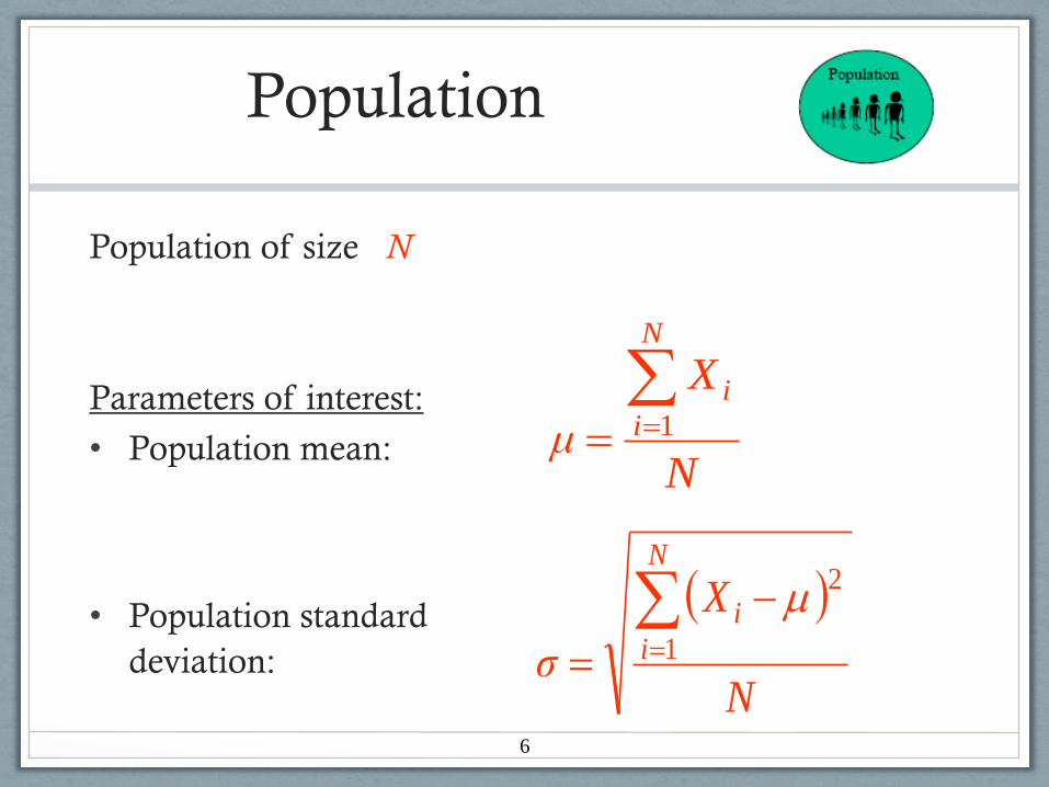
Population

Population of size N

Parameters of interest:

• Population mean:

• Population standard

deviation:

N

X

μ

N

i

i 1

N

X

σ

N

i

i

1

2

Sample

Random sample of size n

Estimates of interest:

Sample mean: best possible estimate of population mean

Sample standard deviation (S or SD):

an estimate of population

standard deviation

7

1

1

2

n

xx

s

n

i

i

n

x

x

n

i

i 1

Now we know how calculate standard deviation but how to use it in

construction of the error bars? We need to know more about its interpretation.

8

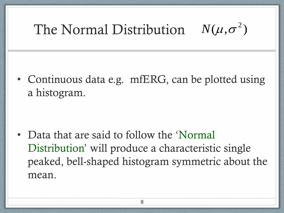
The Normal Distribution

• Continuous data e.g. mfERG, can be plotted using

a histogram.

• Data that are said to follow the ‘Normal

Distribution’ will produce a characteristic single

peaked, bell-shaped histogram symmetric about the

mean.

),( 2N

Normal distribution with mean

and standard deviation

9

Possible values for the variable x

from the population

(16%) (16%)

(68%) 2

),( 2N

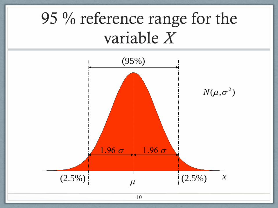
95 % reference range for the

variable X

10

),( 2N

1.96

(95%)

(2.5%) (2.5%)

1.96

x

11

Summary of main properties of the Normal

distribution

• Exactly 95% of the distribution lies between

µ - 1.96 · and µ + 1.96 ·

• This range defines the interval within which 95% of

observations in the population lie.

• Referred to as a reference range or prediction interval

• In practice, µ and are estimated from a sample.

We can use 1.96 ∙ s as an error bar and it will indicate that 95% of subjects

are within such error bars. Or we can use s as error bar and it will indicate

68% of all subjects. These error bars get more accurate with more data,

and they effectively describe the data.

12

Example - reference range

• In our sample of 20 patients we found mean and standard deviation of mfERG:

• A 95% reference range for the mfERG for a person with DM without CSMO and age 25-75 would therefore be:

27.67 - 1.96 · 5.3135 to 27.67 + 1.96 · 5.3135

i.e. 17.26 to 38.08.

Approximately 95% of mfERG of 25-75 yrs patients with DM without CSMO lie in this interval.

5.3135 and27.67 s = = x

Different sample means are obtained

from different samples.

• How good is our estimate of the population mean from

a single sample?

• How large an error might we make if we infer this to be

the population mean?

• Sample means ( ) vary about the population mean (µ)

• This variability can be quantified using the Standard

Error of the Sample Mean (SE)

13

x

Standard error is another measure used to construct error bars. How do we

calculate it and use it properly?

Standard error of the sample mean

14

• Standard Error of the Sample Mean (SE) is given by

(σ estimated by s)

• This is a measure of the precision with which the

population mean is estimated

• SE increases as variability of individual observations (σ)

increases

• SE decreases as sample size (n) increases

n

σSE

SE is a measure of how variable the mean will be, if you repeat the

whole study many times.

Confidence interval for population

mean

We wish to make inference about population mean.

One solution is to find its confidence interval.

• Sample mean ( ) is an estimate of the unknown

population mean (µ)

• A confidence interval for the population mean is a

range of values which we are confident (to some

degree) includes the true value of the population

mean

15

x

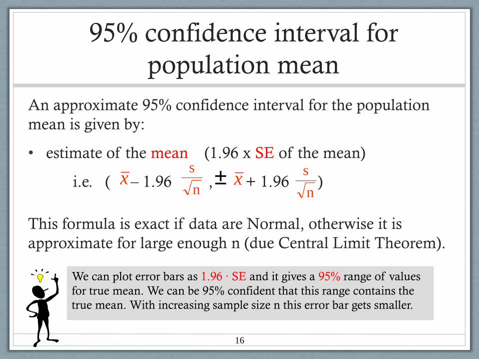
95% confidence interval for

population mean

An approximate 95% confidence interval for the population

mean is given by:

• estimate of the mean (1.96 x SE of the mean)

i.e. ( – 1.96 , + 1.96 )

This formula is exact if data are Normal, otherwise it is

approximate for large enough n (due Central Limit Theorem).

16

±x xn

s

n

s

We can plot error bars as 1.96 ∙ SE and it gives a 95% range of values

for true mean. We can be 95% confident that this range contains the

true mean. With increasing sample size n this error bar gets smaller.

17

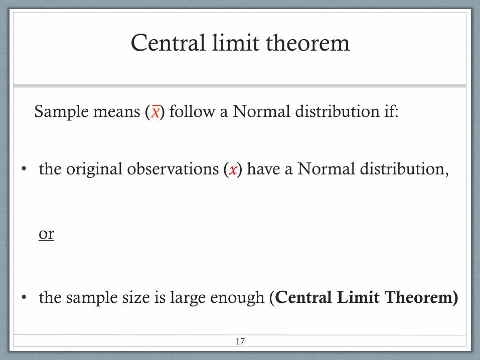
Central limit theorem

Sample means ( ) follow a Normal distribution if:

• the original observations (x) have a Normal distribution,

or

• the sample size is large enough (Central Limit Theorem)

x

18

Central Limit Theorem

2n

2/

x

30n

x

30/

x

Population

1n

Normal

distribution

Skewed

distribution

x xx

1n 2n 30n

Central Limit Theorem: Whatever is the distribution of the variable in the population, the

distribution of the sample mean will be nearly Normal as long as the samples are large enough.

19

Example – confidence interval

• The mean and standard deviation of the mfERG of a

random sample of 20 patients were 27.67 and 5.3135.

• The standard error of the sample mean is estimated by:

• The 95% confidence interval for the population mean is

• i.e.(25.3, 30.0). We are 95% confident that the true

population mean lies within this interval.

1881.120

3135.5

1.1881)*1.96+27.67 1.1881,*1.96-(27.67

Cumming and Finch, 2005

We say we are 95% confident that true

mean is in the CI.

It means that the procedure that we

used does produce a CI that contains

the true mean value in 95%

independent replications.

Figure: The 95 % confidence intervals

for the population mean for 20

independent replications of a study.

Each sample has size n=36.

What we mean by 95%

confidence

Which error bars to use in graphs

Now we know how to construct 4 types of error bars:

• Range i.e. min to max

• Standard deviation: s

• Standard error: SE

• Confidence interval: CI

Which measure is the appropriate one when graphing data?

It depends on the question or aspect of data analysis to be illustrated.

There are 2 situations: descriptive and inferential.

Descriptive error bars

We need descriptive error bars if we want to:

• Indicate the spread in the population.

• We have an observation for a new patient and we

need to know if it is a typical value.

• We want to describe the data at hand.

Can we use error bars:

• Range i.e. min to max ? Yes

• Mean+-S ? Yes

• Mean+-SE ? No

• Mean +-1.96 SE ? No

Holopigian and Bach, 2010

Inferential error bars

We need inferential error bars if our goal is:

• Indicate plausible values of the population mean i.e. to do inference about it.

• Compare two groups of patients i.e. to do inference if the two population means are different.

Can we use error bars:

• Range i.e. Min to max? No

• Mean+-S ? No

• Mean+-SE ? Yes

• Mean +-1.96 SE ? Yes

Holopigian and Bach, 2010

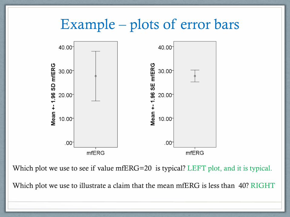
Example – plots of error bars

Which plot we use to see if value mfERG=20 is typical? LEFT plot, and it is typical.

Which plot we use to illustrate a claim that the mean mfERG is less than 40? RIGHT

Summary

• Concepts

• Population and sample

• Population mean and sample mean

• Descriptive statistics and inferential statistics

• They are 2 types of error bars

• Descriptive error bars

• Range, standard deviation

• Inference error bars

• Standard error and confidence interval

• When showing error bars, always describe in the figure legends what they are (e.g. s, or 1.96 SE).

Resources

Books

• Practical statistics for medical research by Douglas G. Altman

• Medical Statistics from Scratch by David Bowers

Journals’ with series on how to do statistics in clinical research

• American Journal of Ophthalmology has Series on Statistics

• British Medical Journal has series Statistics Notes

Papers on “inference by eye”

• Holopigian and Bach, A primer on common statistical errors in clinical ophthalmology,

Doc. Ophthalmology, 2010

• Cumming G, Finch S, Inference by eye: confidence intervals and how to read pictures of

data, Am Psychol 60, 2005

• Cumming G, Fidler F, Vaux DL, Error bars in experimental biology, J Cell Biol 177: 7-

11, 2007

Thank you for your attention

Email: g.czanner@liverpool.ac.uk

Slides can be found on: http://pcwww.liv.ac.uk/~czanner/

Suggestions for topics for future workshops?