Stable Mesh Decimation

Chandrajit BajajDepartment of Computer

SciencesUniversity of Texas at Austin

bajaj@cs.utexas.edu

Andrew GilletteDepartment of MathematicsUniversity of Texas at Austin

agillette@math.utexas.edu

Qin ZhangDepartment of Computer

SciencesUniversity of Texas at Austinzqyork@ices.utexas.edu

ABSTRACTCurrent mesh reduction techniques, while numerous, all pri-marily reduce mesh size by successive element deletion (e.g.edge collapses) with the goal of geometric and topologicalfeature preservation. The choice of geometric error used toguide the reduction process is chosen independent of thefunction the end user aims to calculate, analyze, or adap-tively refine. In this paper, we argue that such a decou-pling of structure from function modeling is often unwiseas small changes in geometry may cause large changes inthe associated function. A stable approach to mesh decima-tion, therefore, ought to be guided primarily by an analysisof functional sensitivity, a property dependent on both theparticular application and the equations used for computa-tion (e.g. integrals, derivatives, or integral/partial differen-tial equations). We present a methodology to elucidate thegeometric sensitivity of functionals via two major functionaldiscretization techniques: Galerkin finite element and dis-crete exterior calculus. A number of examples are given toillustrate the methodology and provide numerical examplesto further substantiate our choices.

1. INTRODUCTIONFor function computations carried out on large meshes, meshdecimation is an essential first step. Mesh decimation tech-niques are distinguished by the cost function they attemptto minimize as they collapse edges in the mesh. In thispaper, we show that given a particular partial differentialequation (PDE) problem, an analysis of the geometric sen-sitivity of the functions involved should guide the choice ofcost function for pre-computation decimation.

We consider such function-guided decimation in two realms:adaptive finite element methods (AFEM) and discrete exte-rior calculus (DEC) methods. There are three main steps insuch methods: formulating a weak version of the governingPDEs, discretizing the problem, and solving the resultinglinear system. Each step introduces a different type of er-ror to the process. Formulating a weak problem may create

what is known as model error. Reducing to a linear sys-tem causes discretization error. Implementing the numericalmethod inevitably causes some solver error.

Adaptive finite element methods aim to control solver errorby selective local refinement of the input mesh (h-adaptivity),the degree of the basis functions (p-adaptivity), or both (hp-adaptivity). While each flavor of adaptive method has metsuccess in particular applications, we will show that their ap-plicability does not immediately transfer to problems thatrequire mesh decimation as a pre-processing step. Mesh dec-imation causes a certain loss of geometric information whileadaptive refinement is an approximation of missing functioninformation. For this reason, it is important that the lossof function information accrued during mesh decimation bebounded a priori so that the adaptive method can have ahope of converging to a meaningful result.

Discrete exterior calculus methods control solver error bydiscretizing the functions and operators of the PDE with re-spect to their algebraic relationships. This type of analysisleads to specific conclusions about where values of the loaddata and solution data should be assigned or computed; inmany cases, values belong most naturally somewhere otherthan mesh vertices, e.g. on mesh edges or at the circumcen-ters of triangles. Therefore, an error bound on function in-formation loss for mesh decimation prior to a DEC methodmust, by necessity, take into account the locations of thesamples of the various variables in the problem.

We describe a framework for selecting an appropriate meshdecimation technique given a PDE and an approach to solv-ing it. The discretization from the AFEM or DEC methodyields a linear system of the form Ax = b whose solution re-quires inverting the matrix A. Our contention is that meshdecimation should be guided by an attempt to avoid largeentries in the matrix A which can make A ill-conditionedand hence destabilize the numerical method.

In Section 2, we discuss prior work on AFEM, DEC, andmesh decimation. In Section 3, we first give a general overviewof AFEM and DEC methods and then explain how each cansuggest a mesh decimation technique through a variety ofexamples. In Section 4, we describe the cost functions as-sociated to two existing techniques as well two novel costfunctions for use in molecular solvation energetics computa-tions. In Section 5, we present initial experimental resultscomparing our technique to prior ones.

Permission to make digital or hard copies of all or part of this work for personal or classroom use is granted without fee provided that copies are not made or distributed for profit or commercial advantage and that copies bear this notice and the full citation on the first page. To copy otherwise, or republish, to post on servers or to redistribute to lists, requires prior specific permission and/or a fee. 2009 SIAM/ACM Joint Conference on Geometric and Physical Modeling (SPM ’09), October 4-9, 2009, San Francisco, CA. Copyright 2009 ACM 978-1-60558-711-0/09/10…$10.00.

277

2. PRIOR WORKWe discuss the three main topics of prior work related to ourapproach: adaptive finite element methods, discrete exteriorcalculus methods, and mesh decimation methods.

Finite element methods (FEM) have witnessed an explosivegrowth both in the literature and in industrial applicationin the past few decades. Adaptive methods [2] have gainedtraction for their ability to increase local accuracy in a so-lution. Beginning with a coarse mesh, AFEM refine by sub-dividing certain elements into smaller pieces (h-adaptivity)[16], increasing the degree of polynomial approximation onsome elements (p-adaptivity) [3], or a combination of thetwo (hp-adaptivity) [14]. Recently AFEM have been ap-plied to computational biology disciplines. Baker et al. haveworked on a parallel implementation of an AFEM to solvethe Poisson-Boltzmann equation [8] which generates a meshof the molecular surface via a subdivision scheme. Recentwork by Chen et al. [12] provides a FEM for the nonlin-ear Poisson-Boltzmann equation with rigorous convergenceestimates.

Discrete Exterior Calculus (DEC) is an attempt to createfrom scratch a discrete theory of differential geometry andtopology whose definitions and theorems mimic their smoothcounterparts. This theoretical foundation allows the canon-ical prescription of a discretization scheme for a given PDEproblem that enforces topological constraints combinatori-ally instead of numerically, thereby providing for increasedrobustness in implementation. This approach has been em-ployed by an increasing number of authors in recent yearsto develop multigrid solvers [9], solve Darcy flow problems[22], and geometrize elasticity [29]. For a complete introduc-tion to DEC theory, see Hirani [21] and Desbrun et al. [15].In this paper, we give a brief introduction to the theory inSection 3 and an example in Section 3.3.

Mesh decimation techniques are abundant in geometry pro-cessing literature. A useful survey of many methods wasgiven by Heckbert and Garland [20] and a more recent bookby Luebke et al. [27] provides a thorough overview of meshsimplification techniques. Bajaj and Schikore [6] have givenan error bounded mesh decimation technique for 2D scalarfield data. We focus on mesh decimation of unstructuredsurface meshes via edge contraction including the approachesof Garland and Heckbert [18] and Lindstrom and Turk [23,24]. These are explained in Section 4.

3. METHODOLOGY FOR ELUCIDATINGGEOMETRY SENSITIVE FUNCTIONALS

We begin with a general problem: find u ∈ V such that

Lu = f on Ω, (1)

where L is a linear operator, V is the appropriate solutionspace for the problem, and Ω is a simplicial complex embed-ded in R3. There are two main techniques used to discretizethis into a linear system: Galerkin methods and DiscreteExterior Calculus (DEC) methods. We describe how eachcould be used and how a mesh decimation technique shouldbe chosen accordingly.

The Galerkin finite element method begins by putting (1)

into the weak form: find u ∈ V such that

a(u, v) = (f, v)L2 ∀v ∈ V, (2)

where a is the operator L phrased as a bilinear form (usuallysymmetric) and f is treated as a functional (f, ·)L2 on V .An appropriate finite dimensional subspace Vh ⊂ V is chosenand an answer to the following discretized problem is sought:find u ∈ Vh such that

a(u, v) = (f, v)L2 ∀v ∈ Vh.

Since Vh is finite-dimensional, we can fix a basis {φi : 1 ≤i ≤ n} of Vh. The size of the basis is proportional to thenumber of elements in the mesh Ω. Write u =

∑nj=1 Ujφj ,

Kij = a(φj , φi) and Fi = (f, φi). Set U = (Uj), K = (Kij)F = (Fi). Then solving (2) over Vh is the same as solvingthe matrix equation

KU = F. (3)

For a proof and detailed discussion, see [11].

A significant amount of care goes into the selection of Vh

to ensure that the method is both well-posed and stable.“Well-posed” means the system has a unique solution and“stable” means there exists a constant C > 0 independent ofh such that

||u − uh||V ≤ C infwh∈Vh

||u − wh||V .

In other words, a method is stable if the error between thetrue solution u and approximate solution uh is boundedabove uniformly by a constant multiple of the minimal ap-proximation error for Vh. The famous Babuska inf-sup con-dition [1] is often used to simultaneously prove both well-posedness and stability of a FEM and hence provide an apriori bound on solver error. We note, however, that thestability error bound does not account for error due to naivemesh decimation.

If the mesh Ω has too many elements, (3) will be too largefor the solver, making decimation necessary. For decimationto be useful, however, it must not create very large or smallentries in K which might make K ill-conditioned. Since theentries of K are a functional a(·, ·) on the basis functions φi,mesh decimation must be guided by the geometry-sensitivecomponents of a as opposed to the geometry of Ω alone.Such components are necessarily problem-specific as we elu-cidate in examples presented in Sections 3.1 and 3.2.

The method of Discrete Exterior Calculus is an alternativeapproach which focuses on correctly discretizing the opera-tor L instead of the solution space V . The viewpoint pro-vided by differential geometry and topology reveals how thisought to be done. Common operators such as grad, curl, anddiv are all manifestations of the exterior derivative operatord in dimensions 1, 2, and 3, respectively. Equations relatingquantities of complementary dimensions, such as the con-stitutive relations in Maxwell’s equations, involve a Hodgestar operator ∗ which provides the canonical mapping. TheLaplacian operator Δ can be written as δd + dδ where δ isthe coderivative operator, defined by δ := ∗d∗. Each opera-tor has a discrete version designed to mimic the propertiesof its smooth counterpart. The discrete versions of the op-erators are written as matrices whose entries depend onlyon the topology and geometry of the mesh Ω.

278

To solve (1), an analysis is made as to the dimension ofu as a k-form based on either the problem context or thetype of operator acting on it. The div operator in 3D, forexample, acts on 2-forms while grad acts on 0-forms. Thevariable u is replaced by a vector �u with one entry for eachk-simplex in the mesh of Ω and the operator L is replacedby its discrete counterpart, written as a matrix L. The load

data f is converted to a vector �f accordingly. This yieldsthe equation

L�u = �f, (4)

which can then be solved by linear methods.

Again, it may be necessary to decimate Ω so that the lin-ear system (4) is tractable on a computer. The size of theentries of L depend heavily on the geometry-sensitive op-erators such as ∗ and δ and less on the topology sensitiveoperators such as d. Therefore, to prevent an ill-conditionedL, mesh decimation must be guided based on the definitionof the discrete operators as opposed to the definition of thesolution space. We discuss an example in Section 3.3.

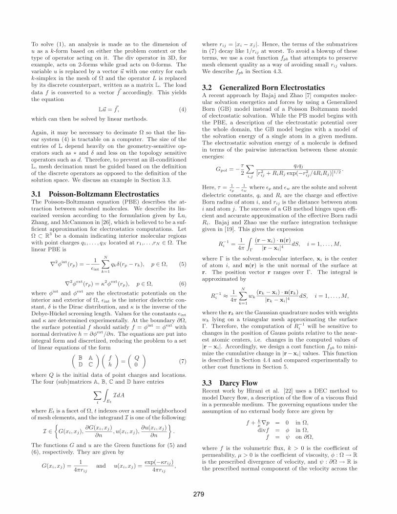
3.1 Poisson-Boltzmann ElectrostaticsThe Poisson-Boltzmann equation (PBE) describes the at-traction between solvated molecules. We describe its lin-earized version according to the formulation given by Lu,Zhang, and McCammon in [26], which is believed to be a suf-ficient approximation for electrostatics computations. LetΩ ⊂ R3 be a domain indicating interior molecular regionswith point charges q1, . . . , qN located at r1,. . . ,rN ∈ Ω. Thelinear PBE is

∇2φint(rp) = − 1

εint

N∑k=1

qkδ(rp − rk), p ∈ Ω, (5)

∇2φext(rp) = κ2φext(rp), p ∈ Ω, (6)

where φint and φext are the electrostatic potentials on theinterior and exterior of Ω, εint is the interior dielectric con-stant, δ is the Dirac distribution, and κ is the inverse of theDebye-Huckel screening length. Values for the constants εint

and κ are determined experimentally. At the boundary ∂Ω,the surface potential f should satisfy f = φint = φext withnormal derivative h = ∂φext/∂n. The equations are put intointegral form and discretized, reducing the problem to a setof linear equations of the form(

B A

D C

) (fh

)=

(Q0

)(7)

where Q is the initial data of point charges and locations.The four (sub)matrices A, B, C and D have entries∑

t

∫Et

IdA

where Et is a facet of Ω, t indexes over a small neighborhoodof mesh elements, and the integrand I is one of the following:

I ∈{

G(xi, xj),∂G(xi, xj)

∂n, u(xi, xj),

∂u(xi, xj)

∂n

}.

The functions G and u are the Green functions for (5) and(6), respectively. They are given by

G(xi, xj) =1

4πrijand u(xi, xj) =

exp(−κrij)

4πrij,

where rij = |xi − xj |. Hence, the terms of the submatricesin (7) decay like 1/rij at worst. To avoid a blowup of theseterms, we use a cost function fpb that attempts to preservemesh element quality as a way of avoiding small rij values.We describe fpb in Section 4.3.

3.2 Generalized Born ElectrostaticsA recent approach by Bajaj and Zhao [7] computes molec-ular solvation energetics and forces by using a GeneralizedBorn (GB) model instead of a Poisson Boltzmann modelof electrostatic solvation. While the PB model begins withthe PBE, a description of the electrostatic potential overthe whole domain, the GB model begins with a model ofthe solvation energy of a single atom in a given medium.The electrostatic solvation energy of a molecule is definedin terms of the pairwise interaction between these atomicenergies:

Gpol = −τ

2

∑i,j

qiqj

[r2ij + RiRj exp(−r2

ij/4RiRj)]1/2.

Here, τ = 1εp

− 1εw

where εp and εw are the solute and solvent

dielectric constants, qi and Ri are the charge and effectiveBorn radius of atom i, and rij is the distance between atomi and atom j. The success of a GB method hinges upon effi-cient and accurate approximation of the effective Born radiiRi. Bajaj and Zhao use the surface integration techniquegiven in [19]. This gives the expression

R−1i =

1

4π

∫Γ

(r − xi) · n(r)

|r − xi|4 dS, i = 1, . . . , M,

where Γ is the solvent-molecular interface, xi is the centerof atom i, and n(r) is the unit normal of the surface atr. The position vector r ranges over Γ. The integral isapproximated by

R−1i ≈ 1

4π

N∑k=1

wk(rk − xi) · n(rk)

|rk − xi|4 dS, i = 1, . . . , M,

where the rk are the Gaussian quadrature nodes with weightswk lying on a triangular mesh approximating the surfaceΓ. Therefore, the computation of R−1

i will be sensitive tochanges in the position of Gauss points relative to the near-est atomic centers, i.e. changes in the computed values of|r− xi|. Accordingly, we design a cost function fgb to mini-mize the cumulative change in |r−xi| values. This functionis described in Section 4.4 and compared experimentally toother cost functions in Section 5.

3.3 Darcy FlowRecent work by Hirani et al. [22] uses a DEC method tomodel Darcy flow, a description of the flow of a viscous fluidin a permeable medium. The governing equations under theassumption of no external body force are given by

f + kμ∇p = 0 in Ω,

divf = φ in Ω,f = ψ on ∂Ω,

where f is the volumetric flux, k > 0 is the coefficient ofpermeability, μ > 0 is the coefficient of viscosity, φ : Ω → R

is the prescribed divergence of velocity, and ψ : ∂Ω → R isthe prescribed normal component of the velocity across the

279

vR

v1

v2

v21

v22 v2

...

v2U

v11 v1

D

v12 v1

...

0c 2

1c2

2c2

Uc2

0c1Dc1

...c 2

...c 11c1 2c1

vR

v21

v22 v2

...

v2U

v11 v1

D

v12 v1

...

vL vL

0c2

1c2

2c2 ...c 2

Uc2

Dc1

...c 12c1

1c1

0c1

v

(a) (b)

Figure 1: Notation for collapse of edge (v1, v2) tov. Black vertices and edges are unchanged in thecollapse while red vertices and dashed edges maychange.

boundary. They discretize the operators ∇ and div basedon DEC theory to arrive at the linear system[ −(μ/k)Mn−1 DT

n−1

Dn−1 0

] [fp

]=

[0φ

].

Here, Dk is the discrete exterior derivative operator that actson k-cochains and Mk is a diagonal matrix representing theHodge Star operator on k-cochains.

We now consider the effect of a priori mesh decimation forthis scheme. The DEC analysis used to derive this methodrequires that the solution [f p]T provide values of the fluxf on (n − 1)-simplicies (i.e. edges in triangle meshes andtriangles in tetrahedral meshes) and values of the pressurep at the circumcenters of n-simplicies.

For the pressure values to have any meaning, the mesh mustbe well-centered meaning the circumcenter of each simplexmust lie in the interior of the simplex. Since this criterionis often violated by meshing schemes (e.g. an obtuse tri-angle is not well-centered), pressure is assigned instead tothe barycenters of n-simplicies. The authors point out thatthe error introduced by this modification prevents the ex-act representation of linear variation of pressure over thedomain. Therefore, an appropriate cost function for thismethod should be weighted to favor the creation of simpli-fied meshes with good quality elements (e.g. elements withgood aspect ratios). This would minimize the distance be-tween the barycenter and circumcenter, making the calcula-tions more robust.

4. DESCRIPTION OF COST FUNCTIONS4.1 Quadratic Error Cost FunctionThe quadric error measure we use comes from Garland andHeckbert [18]. First, an error metric Δ(v) is establishedfor each vertex v, based on the planes P (v) that containthe triangles incident to v. A plane p ∈ P (v) given byax + by + cz + d = 0 is represented as [a b c d]T . Thevertex v is represented as [vx vy vz 1]T . Then the errormetric Δ(v) is defined by

Δ(v) = vT

⎛⎝ ∑

p∈P (v)

ppT

⎞⎠ v.

For a vertex vi, let Qi =∑

p∈P (vi)ppT . Then the cost of

collapsing edge (v1,v2) to some point v is

fqe(v1,v2;v) := vT (Q1 + Q2)v.

We use the publicly available software QSlim [17] to im-plement this cost function. For a given edge, the programattempts to find an optimal placement of v by solving acertain linear system derived from the Qi. If the matrix as-sociated to this system is not invertible, it tries to place voptimally on (v1,v2). If this fails, it sets v to be either v1,v2, or the midpoint of the edge, whichever minimizes fqe.

4.2 Volumetric Error Cost FunctionThe volumetric error measure we use comes from Lindstromand Turk [23, 24]. First, we establish the notation for thesigned volume V of a tetrahedron bounded by a vertex v andthe vertices vti

0 , vti1 , vti

2 of a triangle ti. As before, verticesare written as four component vectors, e.g. v is representedby [vx vy vz 1]T . Then V is defined by

V (v,vti0 ,vti

1 ,vti2 ) =

1

6det(v vti

0 vti1 vti

2 ) =:1

6Gtiv

where Gti is a 1 by 4 matrix defined by the above equation.The cost of collapsing edge (v1,v2) to some point v is

fvol(v1,v2;v) :=1

2vT

(1

18

∑i

GTtiGti

)v,

where i indexes over triangles ti incident to at least one of{v1,v2}. This cost function is ultimately quite similar tofqe except that fqe weights the distance between v and aplane by the area of the triangle defining the plane whilefvol weights it by the square of the triangle area. As isexplained in [23, 24], this weighting better serves the goalof volume preservation. We use a package from the publiclyavailable software TeraScale Browser [25] to implement thiscost function.

4.3 Poisson Boltzmann Cost FunctionIn Section 3.1 we discuss how Poisson Boltzmann (PB) com-putations are sensitive to Gaussian quadrature points com-ing into close proximity. Hence, we define a cost functionfpb which penalizes such occurrences.

We fix the following notation for the collapse of edge (v1,v2)to the point v. Consider the union of triangles incident to v1

or v2. These are the only vertices, edges, and triangles whosegeometry may be changed by the edge collapse. Althoughall these objects lie in R3, their generic connectivity infor-mation is captured in R2 by Figure 1 (a). Taking (v1,v2)to be vertical with v1 at the bottom, the triangle to the left(resp. right) of the edge has vL (vR) as its third vertex.We proceed from vL to vR along the upper (resp. lower)vertices labeling them v1

2, v22, . . ., vU

2 (v11, v2

1, . . ., vD1 (D for

down)). Set v02 := v0

1 := vL and vU+12 := vD+1

1 := vR. Wedenote the centers of the triangles not adjacent to (v1,v2)as

cu2 :=

1

3

(v2 + vu

2 + vu+12

), u = 0, 1, . . . , U,

cd1 :=

1

3

(v1 + vd

1 + vd+11

), d = 0, 1, . . . , D.

280

The collapse operation moves v1 and v2 to v. The result isshown in Figure 1 (b). The {vd

1} and {vu2} are unchanged,

but the new centers are {cu2} and {cd

1} where v replaces v2

or v1 in the expression of the center. Re-index cd1 and cu

2 asci.

If the triangles indexed by the ci are of good quality, meaningnearer-to-equilateral, their Gaussian quadrature points willbe better spaced. We approximate the quality of a triangleT by

q(T ) :=l(T )

s(T )+

maxa(T )

mina(T ),

where l(T ) (resp. s(T )) denotes the longest (shortest) sideand maxa(T ) (resp. mina(T )) denotes its maximum (minu-mum) angle. The best quality triangles have the minimumq value of 2. We denote triangles in Figure 1 by their centerci or ci. The cost function is then defined to be

fpb(v1,v2;v) :=∑

i

q(Tci) − q(Tci).

To further improve element quality, we decimate in stagesand run a quality improvement code based on geometric flow[28] in between stages.

4.4 Generalized Born Cost FunctionIn Section 3.2 we discuss how the Generalized Born (GB)computations are sensitive to changes in the location ofGaussian quadrature points {ci} relative to the atomic cen-ters {xj} of the molecule in question. Hence, we define a costfunction fgb which penalizes edge collapses with a larger cu-mulative change in |ci − xj | values. Since it would be toocomputationally expensive to compute the complete changefor every edge collapse, we use a restricted set of pertinent{ci} and {xj} values described below.

We take the {ci} described in Section 4.3 as our set of per-tinent Gaussian quadrature points. We set {xj} to be thoseatomic centers lying within a fixed distance ρ of either v1 orv2. Since Born radii are on the order of 1-2 A, ρ should beset between 2 and 5 to capture a manageable, non-empty setof nearby atoms. In the future, we will devise a parametersweep to optimize the value of ρ.

We want to minimize the atomic center functional fac

fac :=

∣∣∣∣∣∑i,j

|ci − xj |2 − |ci − xj |2∣∣∣∣∣ ,

which can be re-written as

fac =

∣∣∣∣∣∑i,j

cTi ci − cT

i ci + 2(cTi − cT

i )xj

∣∣∣∣∣ .

All the variables in the above expression are known, savefor the ci which are linear functions of v. We define theGB-dependent cost function to be

fgb(v1,v2;v) := |v1 − v2| + λfac(v1,v2;v).

The first term is used to promote the collapse of shorteredges and thereby improve triangle quality. The weight fac-tor λ is chosen so that the two terms are of the same orderof magnitude.

Figure 2: Top: Surface rendering of mAChE beforedecimation. The original mesh of the surface hasabout 200,000 vertices and 400,000 faces. In theinset, the fine mesh is visible. This pocket region ofthe molecule aids in its biological function. Bottom:The mesh of the pocket after decimation to 25,500faces using fqe (left) and a modified version of fgb

(right).

5. EXPERIMENTAL RESULTS AND CON-CLUSIONS

To test the validity of our claims, we work with MouseAcetylcholinesterase (mAChE). This macromolecule servesan important regulatory function as it terminates the ac-tion of the neurotransmitter acetylcholine (ACh). The ini-tial mesh of the molecular surface is generated from a Pro-tein Data Bank (PDB) [10] file of the molecule using ourin-house software TexMol [13]. We show a picture of theinitial mesh in Figure 2. We decimate this mesh using thecost function fqe and a modified version of fgb which uses fqe

instead of |v1 − v2|. We use a Dynamic Packing Grid datastructure [5] to efficiently compute the set {xj} of nearbycenters for each mesh edge. We set ρ = 5 and λ = 10−8 andcompute the polarized and non-polarized energy for eachmesh using the nFFGB code described in [7]. The meshesare only marginally different as shown in Figure 2 and thusproduce similar energy values as shown in the charts in Fig-ure 3. With further experimentation and parameter sweeps,we believe fgb will begin to out-perform fqe. Still, Figure 3shows that fvol is a decidedly worse choice for non-polarizedenergy computations as it does not respect the functionalsensitivity of the problem. In future work, we will also im-plement fpb and use PB-CFM code by Bajaj and Chen [4]to compute and compare PB energetics.

6. ACKNOWLEDGMENTSWe would like to thank Dr. Peter Lindstrom for his helpwith the TeraScale Browser software and Dr. Wenqi Zhaofor her help with the energetics calculations. This researchwas supported in part by NSF grants DMS-0636643, CNS-0540033 and NIH contracts R01-EB00487, R01-GM074258,R01-GM07308.

281

Figure 3: Effect of cost function used for decimationon computed GB energy values for mAChE.

7. REFERENCES[1] I. Babuska and A. Aziz. Survey lectures on the

mathematical foundations of the finite elementmethod. In The Mathematical Foundations of theFEM with Applications to PDEs, Proc. Sympos., 1972.

[2] I. Babuska, J. Chandra, and J. E. Flaherty. AdaptiveComputational Methods for Partial DifferentialEquations. SIAM, Philadelphia, PA, USA, 1983.

[3] I. Babuska, O. C. Zienkiewicz, J. Gago, and E. R.de A. Oliveira. Accuracy Estimates and AdaptiveRefinements in Finite Element Computations. JohnWiley and Sons, Chichester, 1986.

[4] C. Bajaj and A. Chen. Efficient and accuratehigher-order fast multipole bem for poisson-boltzmannelectrostatics. SIAM J. on Sci. Comp., Submitted.

[5] C. Bajaj, R. Chowdhury, and M. Rasheed. A dynamicdata structure for flexible molecular maintenance andinformatics. In SIAM/ACM GDSPM09, Accepted.

[6] C. Bajaj and D. Schikore. Topology preserving datasimplification with error bounds. Computers andGraphics, 22:3–12(10), 25 February 1998.

[7] C. Bajaj and W. Zhao. Fast molecular solvationenergetics and forces computation. SIAM J. Sci.Comp., Submitted.

[8] N. A. Baker, D. Sept, M. J. Holst, and J. A.McCammon. The adaptive multilevel finite elementsolution of the Poisson-Boltzmann equation onmassively parallel computers. J. Comput. Chem, 21,2000.

[9] W. N. Bell. Algebraic multigrid for discrete differentialforms (dissertation). Technical report, University of

Illinois at Urbana-Champaign, 2008.

[10] H. M. Berman, J. Westbrook, Z. Feng, G. Gilliland,T. Bhat, H. Weissig, I. Shindyalov, and P. Bourne.The Protein Data Bank. Nucleic Acids Research,pages 235–242, 2000.

[11] S. Brenner and L. Scott. The Mathematical Theory ofFinite Element Mehtods. Springer-Verlag, New York,2002.

[12] L. Chen, M. J. Holst, and J. Xu. The finite elementapproximation of the nonlinear poisson-boltzmannequation. SIAM J. Numer. Anal., 45(6):2298–2320,2007.

[13] CVC. TexMol. http://ccvweb.csres.utexas.edu/ccv/projects/project.php?proID=8.

[14] L. Demkowicz. Computing with hp-adaptive finiteelements. Chapman and Hall / CRC, 2007.

[15] M. Desbrun, A. N. Hirani, M. Leok, and J. E.Marsden. Discrete Exterior Calculus.arXiv:math/0508341, 2005.

[16] J. E. Flaherty, M. Shepard, P. Paslow, andD. Vasilakis. Adaptive Methods for Partial DifferentialEquations. SIAM, Philadelphia, PA, USA, 1989.

[17] M. Garland. QSlim. http://graphics.cs.uiuc.edu/∼garland/software/qslim.html, 2004.

[18] M. Garland and P. S. Heckbert. Surface simplificationusing quadric error metrics. In SIGGRAPH ’97, pages209–216, New York, NY, USA, 1997.

[19] A. Ghosh, C. S. Rapp, and R. A. Friesner. Generalizedborn model based on a surface integral formulation.The Journal of Physical Chemistry B,102(52):10983–10990, 1998.

[20] P. Heckbert and M. Garland. Survey of polygonalsurface simplification algorithms. Technical report,Carnegie Mellon University, 1995.

[21] A. N. Hirani. Discrete exterior calculus (dissertation).Technical report, Cal Tech, 2003.

[22] A. N. Hirani, K. B. Nakshatrala, and J. H. Chaudhry.Numerical method for Darcy flow derived usingDiscrete Exterior Calculus. arXiv:0810.3434, 2008.

[23] P. Lindstrom and G. Turk. Fast and memory efficientpolygonal simplification. In VIS ’98, pages 279–286,1998.

[24] P. Lindstrom and G. Turk. Evaluation of memorylesssimplification. IEEE Transactions on Visualizationand Computer Graphics, 5(2):98–115, 1999.

[25] LLNL. TeraScale Browser.https://computing.llnl.gov/vis/terascale.shtml, 2007.

[26] B. Lu, D. Zhang, and J. A. McCammon. Computationof electrostatic forces between solvated moleculesdetermined by the poisson–boltzmann equation usinga boundary element method. Journal of ChemicalPhysics, 122(21):214102–1–7, 2005.

[27] D. Luebke, B. Watson, J. D. Cohen, M. Reddy, andA. Varshney. Level of Detail for 3D Graphics. ElsevierScience Inc., New York, 2002.

[28] G. Xu, Q. Pan, and C. L. Bajaj. Discrete surfacemodelling using partial differential equations. CAGD,23(2):125–145, 2006.

[29] A. Yavari. On geometric discretization of elasticity.Journal of Mathematical Physics, 49(2):1–36, 2008.

282