Stabilization of the Buckling

by High-frequency Excitation

Koji TSUMOTO

(Doctoral Program in Intelligent Interaction Technologies)

Advised by Hiroshi YABUNO

Submitted to the Graduate School of

Systems and Information Engineeringin Partial Fulfillment of the Requirements

for the Degree of Master of Engineeringat the

University of Tsukuba

January 2006

Abstract

Beam is one of fundamental elements in complex structures. It is very significant to clarifyits stability under various circumstances. In particular, the buckling phenomenon charac-terized as a pitchfork bifurcation has accepted much interest by many researchers. In thispaper, we propose a stabilization control method for the first-mode buckling phenomenon inthe clamped-clamped beam without feedback control. We theoretically analyze the stabilityof a buckled beam under high-frequency excitation. It is experimentally clarified that thehigh-frequency excitation shifts the bifurcation point and increases the critical compressiveforce.

Contents

1 Introduction 1

2 Theoretical Analysis 22.1 Analytical model and equation of motion . . . . . . . . . . . . . . . . . . . 22.2 Behavior of a buckled beam under high-frequency excitation . . . . . . . . . 4

2.2.1 Buckling of clamped-clamped beam and mode shape . . . . . . . . . 42.2.2 Derivation of averaged equation using the method of multiple scales 52.2.3 Stability of buckled beam under high-frequency excitation . . . . . . 9

2.3 Postbuckling behavior under high-frequency excitation . . . . . . . . . . . . 13

3 Experiment 163.1 Experimental Setup . . . . . . . . . . . . . . . . . . . . . . . . . . . . . . . 163.2 Experimental result and discussion . . . . . . . . . . . . . . . . . . . . . . . 19

4 Conclusion 29

Acknowledgements 30

Bibliography 31

Related Presentation 31

Appendix A 32

Appendix B 34

i

List of Figures

2.1 Beam subjected to axially high-frequency excitation . . . . . . . . . . . . . 22.2 Comparison between stability in unexcited system and excited system . . . 112.3 Theoretical dependence of the increment of ∆pcr on K(= EI/ρAl4N2) . . . 122.4 Theoretical dependence of the increment of ∆pcr on the amplitude of excitation 122.5 Theoretical bifurcation diagram illustrating the equilibrium points obtained

from averaged equation (2.71) . . . . . . . . . . . . . . . . . . . . . . . . . . 15

3.1 Experimental setup of clamped-clamped beam . . . . . . . . . . . . . . . . 173.2 Picture of experimental setup . . . . . . . . . . . . . . . . . . . . . . . . . . 183.3 Picture of end can fleely move in axial direction . . . . . . . . . . . . . . . . 183.4 Deflection of the beam against the excitation amplitude (N/2π = 18 Hz) . . 203.5 Relationship between deflection of the beam v and axial compressive force P 223.6 Focus on each data of the defleciton v against compressive force P under

excitation in Figure 3.5(b) . . . . . . . . . . . . . . . . . . . . . . . . . . . . 233.7 Relationship between deflection of the beam v and axial compressive force P

under the excitation(Excitation frequency = 20 Hz, Amplitude of excitation= 0.14 mm) . . . . . . . . . . . . . . . . . . . . . . . . . . . . . . . . . . . . 24

3.8 Dependence of the excitation frequency on critical buckling force(a = 0.14mm) . . . . . . . . . . . . . . . . . . . . . . . . . . . . . . . . . . . . . . . . 25

3.9 Behavior of the beam under the excitation condition in the region A(a=0.14mm) . . . . . . . . . . . . . . . . . . . . . . . . . . . . . . . . . . . . . . . . 26

3.10 Dependence of the increment of critical buckling force on the excitation am-plitude (N/2π = 33 Hz) . . . . . . . . . . . . . . . . . . . . . . . . . . . . . 28

B1 Experimental setup of the simply supported beam . . . . . . . . . . . . . . 34B2 Radial bearing of supporting point of beam . . . . . . . . . . . . . . . . . . 35B3 equilibrium region of the deflection of the beam v against the axial compres-

sive force P without excitation . . . . . . . . . . . . . . . . . . . . . . . . . 35B4 Relationship between deflection of the beam v and axial compressive force P

under the excitation . . . . . . . . . . . . . . . . . . . . . . . . . . . . . . . 36

ii

Chapter 1

Introduction

Buckling phenomenon is known as one of most fundamental bifurcation problems. It isproduced when the compressive force makes the stiffness of system zero and the trivialequilibrium state becomes unstable. The stability of beams, which are fundamental elementof complex structure, has been analyzed in many studies. However, there have been fewreports on stabilization method for the buckling. The simplest method is of course toincrease the stiffness of systems. If it is impossible, it is proposed by Pinto et al feedbackcontrol can be utilized to enlarge the stiffness[1].

On the other hand, Chelomei shows the possibility of stabilization control without feed-back for the buckling phenomenon of a straight beam. This method is based on the dynamicstabilization phenomenon such as seen in Kapitza pendulum in which the inverted positionis stabilized with high-frequency excitation[3]. In the dynamic stabilization phenomenon,the force causing destabilization is equivalently cancelled by the high-frequency excitationin the same direction as the destabilized force. In the strategy of Chelomei, a harmonicload is superimposed on the static compressive force[2]. In this research, we deals with thebuckling of a clamped-clamped beam with axial compressive force. Then, the critical forceof the buckling is increased by excitation in the axial direction. By considering the non-linear curvature the governing equation of motion is derived under inextensible condition.Applying the method of multiple scales yields approximate solution and averaged equation.The bifurcation diagrams are obtained in the cases with and without excitation. The in-crease of the critical point of buckling is clarified and the stable buckled deflection is shownunder excitation. Some experiments are performed, and the increase of the critical pointof the buckling is experimentally confirmed. Hysteresis of the steady state which can notbe predicted by theoretical analysis of third order is observed. Furthermore, in a range ofexcitation frequency, chaotic phenomena under high-frequency excitation is experimentallyobserved.

1

Chapter 2

Theoretical Analysis

2.1 Analytical model and equation of motion

x

y

O

l

mv(s,t)

s

P

y'

x'O '

a cos Nt g

Figure 2.1: Beam subjected to axially high-frequency excitation

We consider a clamped-clamped beam at the end mass to which the axial compressiveforce P is applied as shown in Figure 2.1. Periodic excitation for stabilization of buckling isa cos Nt, where a and N are excitation amplitude and frequency, respectively. The notationemployed in this analysis is as follows: t is the time; s is the distance along deformed ornot deformed neutral axis; x and y are the inertial coordinates; u(s, t) and v(s, t) arethe displacements of the centroid at the curve length s, x and y, respectively; and otherparameters are as follows:

l : Length of beam [m]m: End mass [kg]

ρA: Line density of beam [kg/m]E : Young modulus [N/m 2]I : Moment of inertia of cross-sectional area [m4].

Using Bernoulli-Euler beam theory and assuming the inextensible condition, the equationof motion considered until cubic nonlinearity and the associated boundary conditions for

2

the beam are represented as:

ρAv + EI(v′′′′ + v′′′′v′2 + 4v′v′′v′′′ + v′′3)

+ ρAv′′∫ s

l

∫ s

0(v′2 + v′v′)dsds

+ ρAv′∫ s

l(v′2 + v′v′)ds + mv′′

∫ l

0(v′2 + v′v′)ds

+ v′′(

1 +32v′2

)P − ρAaN2 cos Nt{(l − s)v′′ − v′}

− maN2v′′ cos Nt = 0 (2.1)

v∣∣s=0

= v′∣∣s=0

= v∣∣s=l

= v′∣∣s=l

= 0, (2.2)

where [˙] and [′] stand for the derivatives with respect to time t and coordinate s, respectively.The above equation of motion has time varying coefficients and is a Mathieu type. As

mentioned in many articles (for example [6]), parametric resonances can be produced inthe special conditions of the excitation frequency. However, that high-frequency excitationcan stabilize the trivial static unstable equilibrium states and this phenomenon is known as“dynamic stabilization phenomenon.”

Next, we rewrite Eq. (2.1) in the dimensionless form. Using the representative time 1/Nand the representative length l, we set the dimensionless parameters as follows:

t∗ =t

T, s∗ =

s

l, v∗ =

v

l, a∗ =

a

l, m∗ =

m

ρAl,

P ∗ =P

ρAl2N2,K∗ =

EI

ρAl4N2.

Here P ∗ is a dimensionless compressive force, K∗ is a dimensionless flexural rigidity. Equa-tions (2.1) and (2.2) are transformed into dimensionless forms as

v∗ + K∗(v∗′′′′ + v∗′′′′v∗′2 + 4v∗′v∗′′v∗′′′ + v∗′′3)

+ v∗′′∫ s∗

1

∫ s∗

0( ˙v∗′

2+ v∗′v∗′)ds∗ds∗

+ v∗′∫ s∗

1( ˙v∗′

2+ v∗′v∗′)ds∗ + m∗v∗′′

∫ 1

0( ˙v∗′

2+ v∗′v∗′)ds∗

+ v∗′′(

1 +32v∗′2

)P ∗ − a∗ cos t∗{(1 − s∗)v∗′′ − v∗′}

− m∗a∗v∗′′ cos t∗ = 0 (2.3)

v∗∣∣s∗=0

= v∗′∣∣s∗=0

= v∗∣∣s∗=1

= v∗′∣∣s∗=1

= 0, (2.4)

where [˙] and [′] are replaced by ∂∂t∗ and ∂

∂s∗ , respectively.Hereafter, the asterisk( ∗) is omitted for simplification.

3

2.2 Behavior of a buckled beam under high-frequency exci-tation

2.2.1 Buckling of clamped-clamped beam and mode shape

First, by neglecting terms, we analyze the equation of motion in the case without periodicalexcitation for the stabilization control to calculate the mode shape as follows:

v + Pv′′ + Kv′′′′ = 0 (2.5)v(0) = v′(0) = v(1) = v′(1) = 0.

It is possible to separate variables as

v = X(t)φ(s), (2.6)

where φ is the solution of boundary-value problem:

Kφ′′′′ + Pφ′′ − ω2φ = 0 (2.7)φ(0) = φ′(0) = φ(1) = φ′(1) = 0, (2.8)

and X is the ordinary differential equation

X + ω2X = 0. (2.9)

The four eigenvalues in Eq. (2.9) are expressed as follows:

Λ = ±α,±iβ,

(2.10)

where

α =

√−P +

√P 2 + 4Kω2

2K,

β =

√P +

√P 2 + 4Kω2

2K.

The compressive force P for the case of ω = 0, i.e., α = 0, β2 = P/K, corresponds thecritical value for the buckling; hereafter the critical force is expressed by Pcr.

The mode shape when P = Pcr the boundary-value problem is rewritten as

Kφ′′′′ + Pcrφ′′ = 0 (2.11)

φ(0) = φ′(0) = φ(1) = φ′(1) = 0. (2.12)

The general solution can be expressed as

φ = c1 + c2s + c3 cos βs + c4 sin βs,

where c1, c2, c3 and c4 are constant and determined by the boundary conditions. Followingsimultaneous equations

φ(0) = c1 + c3 = 0 (2.13a)φ′(0) = c2 + βc4 = 0 (2.13b)φ(1) = c1 + c2 + c3 cos β + c4 sin β = 0 (2.13c)φ′(1) = c2 − βc3 sin β + βc4 cos β = 0 (2.13d)

4

lead to

c3 = −c1, c4 = − 1β

c2. (2.14)

Substituting Eq. (2.14) into Eqs. (2.13c) and (2.13d),

φ(1) = (1 − cos β)c1 + (1 − 1β

sin β)c2 = 0 (2.15)

φ′(1) = β sin β c1 + (1 − cos β) c2 = 0. (2.16)

For a nontrivial solution, the determinant in Eqs. (2.15) and (2.16) must be zero; that is,∣∣∣∣1 − cos β 1 − 1β sin β

β sin β 1 − cos β

∣∣∣∣ = 2 − 2 cos β − β sinβ = 0.

(2.17)

The parameter β for the buckling point (P = Pcr) is determined by Eq. (2.17). The lowestvalue of β corresponding to the first mode is 2π. Therefore, the critical force Pcr is expressedas follows:

Pcr = β2K = 4π2K. (2.18)

The parameters, c2, c3 and c4, are

c2 = −β(1 − cos β)β − sinβ

c1 = 0

c3 = −c1

c4 =1 − cos β

β − sin βc1 = 0, (2.19)

and the mode shape of the buckling point is obtained as follows:

φ(s) = 1 − cos βs. (2.20)

2.2.2 Derivation of averaged equation using the method of multiple scales

Next, we perform the linear analysis for the effect of axial high-frequency excitation. Theequation of motion without nonlinear terms is as follows:

v + Pv′′ + Kv′′′′ + a cos t{(1 + m − s)v′′ − v′} = 0 (2.21)v(0) = v′(0) = v(1) = v′(1) = 0.

By the method of multiple scales, we analyze the equation of motion (2.21), which includesthe effect of the excitation for the stabilization control. We seek a third-order uniformexpansion as

v = εv1 + ε2v2 + ε3v3, (2.22)

where ε is a small parameter (|ε| � 1) of a book-keeping device. Multiple time scales areintroduced as follows:

t0 = t, t1 = εt, t2 = ε2t. (2.23)

5

We rewrite the compressive force P as

P = Pcr + ∆p, (2.24)

where ∆p is a detuning parameter which expresses the nearness of the compressive force Pfrom the critical force Pcr and ∆p > 0 denotes post buckling case. We perform the scalingof parameters as follows:

a = εa,∆p = ε2∆p, (2.25)

where ˆ stands for O(1). We substitute Eq. (2.22) into Eqs. (2.21) and (2.4). Consideringup to the accuracy of O(ε3) and equating the coefficients of like powers of ε yields:

O(ε) : D20v1 + Pcrv

′′1 + Kv′′′′1 = 0 (2.26)

O(ε2) : D20v2 + Pcrv

′′2 + Kv′′′′2 = −2D0D1v1 + mav′′1 cos t0

+a cos t0{(1 − s)v1′′ − v1

′} (2.27)O(ε3) : D2

0v3 + Pcrv′′3 + Kv′′′′3 = −2D0D1v2 − 2D0D2v1 − D2

1v1

−∆pv′′1 + mav′′2 cos t0

+a cos t0{(1 − s)v2′′ − v2

′}, (2.28)

where Dn = ∂/∂tn. The boundary conditions are

v1(0) = v′1(0) = v1(1) = v′1(1) = 0v2(0) = v′2(0) = v2(1) = v′2(1) = 0v3(0) = v′3(0) = v3(1) = v′3(1) = 0. (2.29)

From Eq. (2.26), v1 can be expressed in the neighborhood of the critical compressive forceas

v1 = X1(t0)Φ1(s). (2.30)

Substituting Eq. (2.30) into Eq. (2.26) and the boundary conditions (2.29) yields

D20X1Φ1 + PcrX1Φ′′

1 + KX1Φ′′′′1 = 0 (2.31)

Φ1(0) = Φ′1(0) = Φ1(1) = Φ′

1(1) = 0. (2.32)

Taking into account the buckling condition (ω = 0), Eq. (2.31) can be rewritten as:

D20X1

X1= −K

Φ′′′′1

Φ1− Pcr

Φ′′1

Φ1= −ω2 = 0. (2.33)

From result of the preceding section, we obtain the mode shape as follows:

Φ1(s) = 1 − cos βs. (2.34)

On the other hand, Eq. (2.33) is also the equation governing the time variation of X1 as

D20X1 = 0. (2.35)

The solution is

X1 = A0(t1, t2)t0 + A1(t1, t2). (2.36)

6

We consider the initial velocity is small as O(ε), D0X1 = O(ε). Then, X1 is not function oft0 and can be expressed as follows:

X1 = A1(t1, t2). (2.37)

The v1 is obtained as

v1 = A1(t1, t2)Φ1(s). (2.38)

Substituting Eq. (2.38) into Eq. (2.27), we obtain the following equation:

D20v2 + Pcrv

′′2 + Kv′′′′2 =

a

2[{(1 − s)Φ1

′′ − Φ1′} + mΦ′′

1

]A1(t1, t2)eit0 + c.c., (2.39)

where c.c. denotes the complex conjugate of the preceding terms. Hereafter, c.c. is utilizedas the same meaning. Because this equation is linear, a particular solution of v2 can bewritten as follows:

v2 = aΦ2(s)A1(t1, t2)eit0 + c.c. (2.40)

Substituting Eq. (2.40) into Eq. (2.39) yields

KΦ′′′′2 + PcrΦ′′

2 − Φ2

=12{(1 − s)Φ1

′′ − Φ1′} +

12mΦ′′

1,

=12

(β2 cos βs − β sin βs − β2s cos βs

)+

12mβ2 cos βs. (2.41)

Associated boundary condition is

Φ2(0) = Φ′2(0) = Φ2(1) = Φ′

2(1) = 0. (2.42)

The general solution of Φ2 is expressed as

Φ2 = Φ2 + Φ2p, (2.43)

where Φ2 and Φ2p are the homogeneous and particular solutions, respectively. Letting Φ2p

as

Φ2p = c5 cos βs + c6 sin βs + c7s cos βs (2.44)

and substituting Eq. (2.44) into Eq. (2.41) yields

K{β4c5 cos βs + β3(βc6 + 4c7) sin βs + β4c7s cos βs}+Pcr{−β2c5 cos βs − β(βc6 + 2c7) sin βs − β2c7s cos βs}−(c5 cos βs + c6 sin βs + c7s cos βs)

=12{β2 cos βs − β sin βs − β2s cos βs}

+12mβ2 cos βs. (2.45)

Taking into account β2 = Pcr/K, the coefficients of Φ2p are obtained as:

c5 = −12β2(1 + m), c6 =

(2K − 1)β5 + β3 + β

2(β4 − β2 − 1), c7 =

−β2

2(β4 − β2 − 1). (2.46)

7

Next, we seek the homogeneous solution Φ2 by examining

KΦ′′′′2 + 4PcrΦ′′

2 − Φ2 = 0. (2.47)

The eigenfunction is governed with

Kη4 + Pcrη2 − 1 = 0, (2.48)

and Φ2 is expressed as follows:

Φ2 = b1 cos qs + b2 sin qs + b3 cosh ps + b4 sinh ps, (2.49)

where

p =

√−Pcr +

√Pcr

2 + 4K2K

,

q =

√Pcr +

√Pcr

2 + 4K2K

.

The general solution of Φ2 can be expressed as

Φ2 = b1 cos qs + b2 sin qs + b3 cosh ps + b4 sinh ps

+c5 cos βs + c6 sin βs + c7s cos βs. (2.50)

Using the boundary conditions, we obtain the following equations:

Φ2(0) = b1 + b3 + c5 = 0Φ′

2(0) = qb2 + pb4 + βc6 + c7 = 0Φ2(1) = b1 cos q + b2 sin q + b3 cosh p + b4 sinh p + c5 + c7 = 0Φ′

2(1) = −qb1 sin q + qb2 cos q + pb3 sinh p + pb4 cosh p + βc6 + c7 = 0. (2.51)

Solving these simultaneous equations, we determine b1, b2, b3 and b4, which are shown inAppendix A. The general solution of v2 can be expressed as

v2 = a{A1(t1, t2)eit0 + c.c.}Φ2. (2.52)

Inserting the general solution of v2 into Eq. (2.28) gives

D20v3 + Pcrv

′′3 + Kv′′′′3

= −D21A1Φ1 − Pcr∆pA1Φ1

′′ +12a2A1{(1 + m − s)Φ2

′′ − Φ2′}

+c.c. + n.s.t., (2.53)

where n.s.t. stands for terms not produce secular terms in v3. We focus on only the particu-lar solution by DC component because we don’t need to consider the periodical componentsto analyze the buckling problem which is a static unstable phenomenon. The particular so-lution can be in the form:

v3p = Φ3DC(t1, t2, s) + · · ·.(2.54)

8

Substituting Eq. (2.54) into Eq. (2.53), we obtain

KΦ′′′′3DC + PcrΦ′′

3DC = −D21A1Φ1 − ∆pA1Φ1

′′

+12a2A1{(1 + m − s)Φ2

′′ − Φ2′}. (2.55)

Associated boundary conditions are

Φ3DC(0) = Φ′3DC(0) = Φ3DC(1) = Φ′

3DC(1) = 0. (2.56)

In order to determine the solvability condition of Eq. (2.55), we multiply the both sides ofEq. (2.55) by Φ1 and integrate by s from 0 to 1. By using the boundary conditions (2.32)and (2.56), Eq. (2.55) becomes∫ 1

0Φ2

1ds · D21A1 +

∫ 1

0Φ1Φ1

′′ds · ∆pA1

−12

∫ 1

0Φ1{(1 + m − s)Φ2

′′ − Φ2′}ds · a2A1 = 0. (2.57)

The above equation can be simplified as

D21A1 + (C1a

2 − C2∆p)A1 = 0, (2.58)

where

C1 = −12

∫ 1

0Φ1{(1 + m − s)Φ2

′′ − Φ2′}ds

/∫ 1

0Φ2

1ds

C2 = −∫ 1

0Φ1Φ1

′′ds

/∫ 1

0Φ2

1ds.

The parameter C2 is a positive constant. C1 implicitly depends on the dimensionlessflexural rigidity K. Equation (2.58) is a differential equation with respect to the slow timescale t1. This means that A1 changes slowly compared with excitation.

2.2.3 Stability of buckled beam under high-frequency excitation

From the above result, we can express the approximate solution of Eq. (2.21) in theneighborhood of the critical point for the first mode buckling as follows:

v ≈ εv1 = εA1Φ1 = A1(t)Φ1(s) = A1(t)(1 − cos βs). (2.59)

The equation governing the dynamics of deflection A1(= εA1) is derived by multiplying Eq.(2.58) by ε3 and is expressed as

d2A1

dt2+ (C1a

2 − C2∆p)A1 = 0. (2.60)

and β is the smallest value of Eq. (2.17). Equation (2.60) enables us to perform the stabilityanalysis of the trivial equilibrium point under the excitation. The sign of the coefficient ofthe second term in the left-hand side kequiv i.e. equivalent stiffness, determines the stability.When the sign is positive and negative, the trivial equilibrium point is stable and unstable,respectively. In the case of zero coefficient, the system is in the critical for the buckling.

In the case without excitation (a = 0), the sign of the coefficient of the second term isdetermined by the sign of ∆p and in the critical point (P = Pcr), ∆p is equal to 0. So, the

9

critical point without excitation is obtained as ∆p = 0, or P = Pcr. Bifurcation diagram inthe case without excitation is shown in Figure 2.2(a).

In the case with excitation (a > 0), we can find that the effect of the excitation inhibitsthe occurrence of the buckling by increasing the equivalent stiffness. The ∆pcr is defined as

∆pcr ≡ C1a2

C2(> 0), (2.61)

When ∆p = ∆pcr in the case with excitation kequiv is equal to zero. Eq. (2.61) indicatesthe amount of the increase of the critical buckling force by the excitation.

Figure 2.2(a) and 2.2(b) show the stability of the trivial equilibrium points in the caseswithout and with excitation, respectively. The solid and dashed lines stand for the stableand unstable equilibrium points, respectively. In the case without excitation, the criticalpoint is P = Pcr. It is clarified from Figure 2.2(b) that the excitation increases the criticalpoint. The critical point is shifted to Pcr+∆pcr = 2.29×10−4 in the subsequent experiment.

Next, Figure 2.3 shows between ∆pcr against K. Here, the amplitude of the excitationis 3.11 × 10−4. Recalling K = EI/ρAl4N2, K is inversely proportional to the square ofN . Decreasing of K corresponds to increasing of N and vice versa. With this discussion inmind, the critical buckling force is increased with the excitation frequency. The dependenceof ∆pcr on the excitation amplitude is shown in Figure 2.4. The critical buckling force isalso increased with the excitation amplitude.

10

-100

0

50

100

-1.5 -1.0 -0.5 0.0 0.5 1.0 1.5 10-3

10-3

∆p

v

-50

Critical point

(a) Stability of the trivial equilibrium points against ∆pcr

without excitation

-100

0

50

100

-1.5 -1.0 -0.5 0.0 0.5 1.0 1.5

10-3

-50

10-3

∆p

v

∆pcr

Critical point

(b) Stability of the trivial equilibrium points against ∆pcr

under excitation (N=33Hz)

Figure 2.2: Comparison between stability in unexcited system and excited system

11

46.4444

46.4442

46.4440

46.4438

46.4436

46.4434

46.4432

1.00.80.60.40.20.0

10-6

K

∆pcr

Figure 2.3: Theoretical dependence of the increment of ∆pcr on K(= EI/ρAl4N2)

0.14

0.12

0.10

0.08

0.06

0.04

0.02

0.00

140120100806040200 10-6

∆pcr

a

Figure 2.4: Theoretical dependence of the increment of ∆pcr on the amplitude of excitation

12

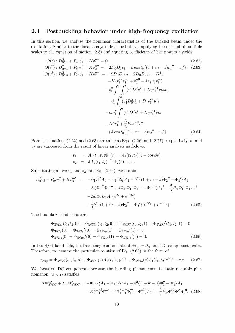
2.3 Postbuckling behavior under high-frequency excitation

In this section, we analyze the nonlinear characteristics of the buckled beam under theexcitation. Similar to the linear analysis described above, applying the method of multiplescales to the equation of motion (2.3) and equating coefficients of like powers ε yields

O(ε) : D20v1 + Pcrv

′′1 + Kv′′′′1 = 0 (2.62)

O(ε2) : D20v2 + Pcrv

′′2 + Kv′′′′2 = −2D0D1v1 − a cos t0{(1 + m − s)v1

′′ − v1′} (2.63)

O(ε3) : D20v3 + Pcrv

′′3 + Kv′′′′3 = −2D0D1v2 − 2D0D2v1 − D2

1v1

−K(v′12v′′′′1 + v′′1

3 − 4v′1v′′1v′′′1 )

−v′′1

∫ s

1

∫ s

0(v′1D

20v

′1 + D0v

′12)dsds

−v′1

∫ s

1(v′1D

20v

′1 + D0v

′12)ds

−mv′′1

∫ s

1(v′1D

20v

′1 + D0v

′12)ds

−∆pv′′1 +32Pcrv

′12v′′1

+a cos t0{(1 + m − s)v2′′ − v2

′}. (2.64)

Because equations (2.62) and (2.63) are same as Eqs. (2.26) and (2.27), respectively, v1 andv2 are expressed from the result of linear analysis as follows:

v1 = A1(t1, t2)Φ1(s) = A1(t1, t2)(1 − cos βs)v2 = aA1(t1, t2)eit0Φ2(s) + c.c.

Substituting above v1 and v2 into Eq. (2.64), we obtain

D20v3 + Pcrv

′′3 + Kv′′′′3 = −Φ1D

21A1 − Φ1

′′∆pA1 + a2{(1 + m − s)Φ2′′ − Φ2

′}A1

−K(Φ1′2Φ1

′′′′ + 4Φ1′Φ1

′′Φ1′′′ + Φ1

′′3)A13 − 3

2PcrΦ′

12Φ′′

1A13

−2iaΦ2D1A1(eit0 + e−it0)

+12a2{(1 + m − s)Φ2

′′ − Φ2′}(e2it0 + e−2it0). (2.65)

The boundary conditions are

Φ3NDC(t1, t2, 0) = Φ3NDC′(t1, t2, 0) = Φ3NDC(t1, t2, 1) = Φ3NDC

′(t1, t2, 1) = 0Φ3Nt0(0) = Φ3Nt0

′(0) = Φ3Nt0(1) = Φ3Nt0′(1) = 0

Φ3N2t0(0) = Φ3N2t0′(0) = Φ3N2t0(1) = Φ3N2t0

′(1) = 0. (2.66)

In the right-hand side, the frequency components of ±t0, ±2t0 and DC components exist.Therefore, we assume the particular solution of Eq. (2.65) in the form of

v3np = Φ3NDC(t1, t2, s) + Φ3Nt0(s)A1(t1, t2)eit0 + Φ3N2t0(s)A1(t1, t2)e2it0 + c.c. (2.67)

We focus on DC components because the buckling phenomenon is static unstable phe-nomenon. Φ3NDC satisfies

KΦ′′′′3NDC + PcrΦ′′

3NDC = −Φ1D21A1 − Φ1

′′∆pA1 + a2{(1+m− s)Φ′′2 − Φ′

2}A1

−K(Φ′12Φ′′′′

1 + 4Φ′1Φ

′′1Φ

′′′1 + Φ′′

13)A1

3 − 32PcrΦ′

12Φ′′

1A13. (2.68)

13

Multiplying Eq. (2.68) by Φ1, integrating the result from s=0 to s=1, and taking intoaccount Eq. (2.66), the solvability condition of the boundary-value problem of Eqs. (2.68)and (2.66) can be expressed as

D21A1 + (C1∆p − C2a

2)A1 + (C3K + C4Pcr)A13 = 0, (2.69)

where

C1 =∫ 1

0Φ1Φ1

′′ds

/∫ 1

0Φ1

2ds

C2 =∫ 1

0Φ1{(1+m− s)Φ2

′′ − Φ2′}ds

/∫ 1

0Φ1

2ds

C3 =∫ 1

0Φ1(Φ1

′2Φ1′′′′ + 4Φ1

′Φ1′′Φ1

′′′ + Φ1′′3)ds

/ ∫ 1

0Φ1

2ds

C4 =32

∫ 1

0Φ1Φ′

12Φ′′

1Φ1ds

/∫ 1

0Φ1

2ds. (2.70)

Furthermore, taking into account Eq. (2.59) and A1 = εA1, we obtain the averaged equationconsidered up to cubic nonlinearity

d2A1

dt2+ (C1∆p − C2a

2)A + (C3K + C4Pcr)A3 = 0, (2.71)

where A indicates the deflection at the midpoint of the beam. This equation governsmodulation of shape of the beam. This averaged equation governed with slow time t1expresses the dynamics of the deflection of a beam. Equation (2.71) is autonomous equationand makes it much easier to perform the bifurcation analysis. As it appears, the linear partof this equation is identical to Eq. (2.60). The equilibrium points and their stability areexamined from Eq. (2.71). Figure 2.5 is the bifurcation diagram which is the relationshipbetween the equilibrium points and the axial compressive force. Figure thbif-no shows thatin the case without excitation. When ∆p < 0 or P < Pcr, the trivial equilibrium v = 0is stable, whereas when ∆p > 0 or P > Pcr, there are two stable nontrivial equilibriaobtained by cubic nonlinearity and there is the unstable trivial equilibrium in-between.This bifurcation is supercritical pitchfork bifurcation.

Figure 2.5(b) is the bifurcation diagram under high-frequency excitation. The excitationamplitude a and frequency N/2π are 3.11 × 10−4 and 33Hz, respectively; this excitationcondition corresponds to that in subsequent experiment. The shift of the critical point isproduced as predicted by linear theory in the previous section. Every nontrivial equilibriumpoint is stable. In the area of 0 < ∆p < 2.29 × 10−4, there are two nontrivial stableequilibrium points and one trivial unstable equilibrium point in the case without excitation.However, in this region there is only one trivial stable equilibrium point by the excitation.Hence, the avoidance of the buckling by high-frequency excitation is anticipated in thatarea.

14

-100

0

50

100

-1.5 -1.0 -0.5 0.0 0.5 1.0 1.5 10-3

10-3

∆p

v

-50

(a) Theoretical bifurcation of the beam v against ∆pcr

without excitation

-100

0

50

100

-1.5 -1.0 -0.5 0.0 0.5 1.0 1.5

10-3

-50

10-3

∆p

v

(b) Theoretical bifurcation of the beam v against ∆pcr

under excitation (N/2π=33Hz)

Figure 2.5: Theoretical bifurcation diagram illustrating the equilibrium points obtainedfrom averaged equation (2.71)

15

Chapter 3

Experiment

3.1 Experimental Setup

We experimentally investigate the increase of critical buckling force of the beam by high-frequency excitation. In Figure 3.1, we show the experimental setup. The beam is rigidlyclamped at the both ends. The beam has a length of 450 mm. The beam width and beamthickness are 10 mm and 0.7 mm, respectively. The first natural frequency is 12.55 Hz, andsecond one is 34.5 Hz. The boundary condition is clamped-clamped. One end is fixed andthe other can freely move in the axial direction. The movable end has mass of 0.51 kg. Thestatic compressive force is applied to the mass by linear motors (SHOWA Electric Wire &Cable Corp., 26-02R). Force of the motor is proportional to the input current to the motor.The current is produced by a power supply unit (KIKUSUI Corp., PBX40-10). When thecompressive force is more than the critical force Pcr, the beam is buckled. Then the parthatched in Figure 3.1 is excited by the shaker (EMIC Corp., 371-A) in the axial direction.The excitation amplitude and frequency are adjusted by a function generator (TOA Corp.,FS-2201). The laser displacement sensors (KEYENCE Corp., LB-01) are not used for thecontrol, but for collecting experimental data. And the sensor 2 measuring the deflection ofthe beam is located at quarter length of the beam from the fixed end. The values of theparameters corresponding to the preceding theoretical analysis are

l : 4.50 ×10−1 mm : 5.1 ×10−1 kg

ρA : 6.21 ×10−2 kg/mE : 1.11 ×1011 N/m2

I : 2.86 ×10−13 m4.

16

FFT analyzer

Sensor

Slide bearing

Displacementsensor 2

Beam

Function generator

Power amplifier

Shaker

amplifier

Slidebearing

Displacementsensor 1

Linear motor

DC/CC power supply

SensorCurrent

This part is excited

Figure 3.1: Experimental setup of clamped-clamped beam

17

Shaker

Linear motors Beam

Figure 3.2: Picture of experimental setup

Beam

Slide bearing

Figure 3.3: Picture of end can fleely move in axial direction

18

3.2 Experimental result and discussion

First, we apply the compressive force and measure the critical compressive force Pcr withoutexcitation. Then, Pcr is 5.925 N.

Next, we observe the deflection of the buckled beam under excitation. In this experiment,we keep the excitation frequency constant (N/2π =18 Hz), where we manually increase theamplitude of the excitation. Figures 3.4(a) and 3.4(b) show the time history of the deflectionof the beam and that of the excitation, respectively. In these figures, the beam is buckled inthe initial state. We start exciting the beam at t = 3s and gradually increase the excitationamplitude until a =0.29 mm. When the amplitude becomes 0.27 mm, the transient state ofthe beam starts. Finally, the buckled beam is stabilized in the neighborhood of the trivialequilibrium point which is unstable in the case without control.

19

10

8

6

4

2

0

-2

-4

v [m

m]

302520151050

t [s]

(a) Time history of the deflection of the beam v

-0.4

-0.2

0.0

0.2

0.4

Am

pli

tude

[mm

]

302520151050

t [s]

(b) Time history of the excitation amplitude

Figure 3.4: Deflection of the beam against the excitation amplitude (N/2π = 18 Hz)

20

Figure 3.5 shows the experimental bifurcation diagram expressing the relationship be-tween the compressive force P and the deflection of the beam v at a quarter of the beamspan from the fixed end. In the case without excitation, it is seen from Figure 3.5(a) thatthe beam is tend to bend to the positive direction because the beam has geometrically im-perfection and it is imperfect supercritical pitchfork bifurcation. This result qualitativelycorresponds to the theoretical bifurcation diagram of Figure 2.5(a) except for the imperfec-tion. The critical buckling force is 5.925 N in experiment, whereas theoretical prediction is6.174 N.

Figure 3.6(a) shows the experimental result under the excitation. The excitation am-plitude and frequency are a = 1.4×10−4m, N/2π = 33Hz, respectively. In this figure, �represents the plot in the quasistationary forward sweep of P . � stands for the quasistation-ary backward sweep of P from the upper right endpoint. � stands for the quasistationarybackward sweep of P from the lower right endpoint. As theoretically predicted in the linearanalysis, we confirm critical point for the buckling is shifted to 6.186 N from 5.925 N by theexcitation, or the critical buckling force increase 0.261 N. However, we observe the nonlin-ear characteristic different from theoretical analysis. In the nonlinear theoretical analysis,the excitation shifts the supercritical pitchfork bifurcation into the right direction on thebifurcation diagram. In the left-hand side of the increased critical force, only stable triv-ial equilibrium point exists. In the right-hand side, the unstable trivial equilibrium pointcoexists with two stable nontrivial ones.

As can be seen from the experiment result Figure 3.5(b), in the left region of the increasedcritical force, two stable nontrivial ones coexist the trivial stable equilibrium point. In theregion, there are five equilibrium points because there must be an unstable equilibriumpoint between two stable ones. So it is derived from the analysis considering up to fifthnonlinear terms. We do not mention the nonlinear property more because we perform thenonlinear analysis considering up to cubic nonlinearity.

21

-40

-30

-20

-10

0

10

20

30v

[mm

]

6.46.26.05.85.6

P [N]

(a) Without excitation

-40

-30

-20

-10

0

10

20

30

v [m

m]

6.46.26.05.85.6

P [N]

(b) With excitation (excitation frequency = 33 Hz, excita-tion amplitude = 0.14 mm)

Figure 3.5: Relationship between deflection of the beam v and axial compressive force P

22

-40

-30

-20

-10

0

10

20

30

6.46.26.05.85.6

v [m

m]

P [N]

(a) Increase P

-30

-20

-10

0

10

20

6.46.26.05.85.6

v [m

m]

P [N]P

(b) Decrease P (Initial condition of v is theupper right end point)

-30

-20

-10

0

10

20

6.46.26.05.85.6

v [m

m]

P [N]

(c) Decrease P (Initial condition of v is thelower right end point)

Figure 3.6: Focus on each data of the defleciton v against compressive force P underexcitation in Figure 3.5(b)

23

Additionally we examine the case when the excitation frequency is changed to 20 Hzunder the same excitation amplitude. We draw the result in Figure 3.7(a) in which Figure3.7(b) is the extended figure of the fragment B. The symbols stand for the same way of thesweep of P same as Figure 3.2. The increase of the critical buckling force is less than inthe case of 33 Hz. The critical buckling force is shifted to 5.991 N or increment of criticalvalue is 0.066 N.

-40

-30

-20

-10

0

10

20

30

6.46.26.05.85.6

P [N]

v [m

m]

B

(a) Bifurcation diagram illustrating the rela-tionship between the deflection of the beamv and the compressive force P . Excitationparameters are as follows: a = 0.14 mm,N/2π = 20 Hz.

-15

-10

-5

0

5

10

15

6.106.056.005.955.90

P [N]

v [m

m]

(b) The enlarged figure of the fragment B in fig-ure 3.7(a)

Figure 3.7: Relationship between deflection of the beam v and axial compressive force Punder the excitation(Excitation frequency = 20 Hz, Amplitude of excitation = 0.14 mm)

We investigate change of the critical buckling force depending on the excitation frequency,under the constant excitation amplitude. Figure 3.8 shows the relationship between the ex-citation frequency N and the difference ∆p between the compressive force P and the criticalforce Pcr without excitation. Experimental results are in good qualitatively agreement with

24

theoretical ones as shown by the solid curve.In the region A, however, we could not find the critical buckling force because the beam

oscillates with various frequency which is not theoretically predicted. We show the behaviorof the beam under an excitation frequency in the region A of Figs. 3.2. The excitationamplitude and frequency are a = 0.14 mm, N/2π = 29 Hz, respectively, and the compressiveforce is 6.05 N which is anticipated neighborhood of the critical force from other results.Figure 3.9(a) shows the time history of the deflection of the beam. In this figure, excitationfrequency is 29 Hz, but the biggest frequency component is 1.95 Hz, and other frequencycomponents also exist.

0.25

0.20

0.15

0.10

0.05

0.00

302520151050

N / 2π [Hz]

∆pcr

[N

]

A

Figure 3.8: Dependence of the excitation frequency on critical buckling force(a = 0.14 mm)

25

-8

-6

-4

-2

0

2

4

6

8

v [m

m]

2.52.01.51.00.50.0

t [s]

(a) Time history of the deflection of the beam v

2.5

2.0

1.5

1.0

0.5

0.0

Po

wer

sp

ectr

um

[m

m]

403020100

N / 2π [Hz]

1.95Hz

3.9Hz23.5Hz

23.9Hz

27.05Hz

29Hz

30.95Hz

(b) Power spectrum of the deflection of the beamv

0.16

0.14

0.12

0.10

0.08

0.06

0.04

0.02

0.00

a [

mm

]

403020100

N / 2π [Hz]

(c) Power spectrum of the excitation

Figure 3.9: Behavior of the beam under the excitation condition in the region A(a=0.14mm)

26

27

0.25

0.20

0.15

0.10

0.05

0.00

0.140.120.100.080.060.040.020.00

∆pcr

[N

]

a [mm]

Figure 3.10: Dependence of the increment of critical buckling force on the excitation am-plitude (N/2π = 33 Hz)

Finally, we investigate change of the critical buckling force depending on the excitationamplitude under the constant excitation frequency(33 Hz). Figure 3.10 shows the rela-tionship between the critical buckling force and the amplitude of the excitation. In thisexperiment the frequency is kept 33 Hz. The critical buckling force is monotonically in-creased with the excitation amplitude. The experimental results quantitatively correspondswell to the theoretical ones.

28

Chapter 4

Conclusion

In this research, we proposed a stabilization method of buckled beam without feedbackcontrol. The dynamic stabilization phenomenon under the high-frequency excitation isutilized and the critical buckling point is shifted to the larger value than that in the casewithout excitation.

It is theoretically clarified that the axial excitation increases equivalently the stiffness ofthe beam and makes it possible to raise the critical compressive force for the buckling. Thenonautonomous equation of motion is transformed into an autonomous equation by usingthe method of multiple time scales introducing three time scales. The autonomous equationenables us to perform nonlinear analysis and gives the approximate solution of the equationof the motion of axially compressed under high-frequency excitation. Then, the effect ofthe high-frequency excitation for increasing the critical buckling force is analytically clari-fied. Furthermore, experimental results confirm the increase of the critical buckling pointunder excitation. However, nonlinear characteristics under the excitation is different fromtheoretical ones. Namely, hysteresis of the equilibrium points in the bifurcation diagramis observed. Also, in a frequency range of the excitation, the beam exhibits modulatedbehavior.

29

Acknowledgements

I would like to express my sincere appreciation to Professor Hiroshi Yabuno who has exploredand given me the opportunity to make a start on this study. This work would not havecompleted without his unstinting support.

I would also like to express my gratitude to Professor Nobuharu Aoshima not only for hiswarm assistance, but accurate and adequate advice thorough out my career.

I am thankful to adviser Professor Youhei Kawamura who have been like my reliable elderbrother who had let me learn and assimilate many things from him.

I would also like to acknowledge Mr. Yohta Kunitoh, the colleague of YABUNO LAB andMr. Mamoru Tsurushima, and all the other junior/senior member of AOSHIMA/YABUNOLAB, who have been very helpful.

Lastly, I am deeply grateful to my parents who have kept supporting me in many waysthroughout my long student life.

30

Bibliography

[1] Pinto, O. C., Goncalves, P. B.: Active non-linear control of buckling and vibrations ofa flexible buckled beam. Chaos Solitons and Fractals, 14, 227-329 (2002)

[2] Chelomei, V. N.: On the possibility of increasing the stability of elastic systems by usingvibration. Doklady Akademii Nauk SSSR, 110(3), 345-347 (1956)[in Russian].

[3] P. L. Kapitza.: Collected Papers by P.L. Kapitza. Perfamon Press, London, 2, 714-726(1965)

[4] Yabuno, H., Miura, M., Aoshima, N.: Bifurcation in an Inverted Pendulum with TiltedHigh-Frequency Excitation (Analytical and Experimental Investigations on Symmetry-Breaking of the Bifurcation). J Sound Vib, 273, 493-513 (2004)

[5] Yabuno, H., Goto, K., Aoshima, N.: Swing-Up and Stabilization of an UnderactuatedManipulator without State Feedback of Free Joint. IEEE Transactions on Robotics andAutomation, 20, 359-365 (2004)

[6] Nayfeh, A. H. and Mook, D. T.: Nonlinear Oscillations. Wiley, New York, 21-26 (1979)

[7] Blekhman, I. I.: Vibrational Mechanics. World Scientific, Singapore (2000)

[8] Yabuno, H., Oowada, R., Aoshima, N.: Effect of Coulomb damping on buckling of asimply supported beam. Proc. of DETC99, Las Vegas, NV, September (1999)

[9] Tcherniak, D. M., Thomsen, J. J.: Slow effects of fast harmonic excitation elastic struc-tures. Nonliner Dynamics, 17, 227-246 (1998)

[10] Tcherniak, D. M.: The influence of fast excitation on a continuous system. J SoundVib, 227(2), 343-360 (1999)

[11] Thomsen, J. J.: Theories and experiments on the stiffening effect of high-frequencyexcitation for continuous elastic systems. J Sound Vib, 260, 117-139 (2002)

[12] Thomsen, J. J.: Slow high-frequency effects in mechanics: problems, solutions, poten-tials. Proc. of ENOC-2005, Eindhoven, August 7-12, 143-193 (2005)

[13] Jensen, J. S., Tcherniak, D. M., Thomsen, J. J.: Stiffening effecs of high-frequencyexcitation: experiments for an axially loaded beam. Journal of Applied Mechanics, 67,397-402 (1999)

[14] Jensen J. S.: Buckling of an elastic beam with added high-frequency excitation. Non-linear Dynamics, 35(2), 217-227 (2000)

[15] Champneys, A. R., Fraser, W. B.: The ‘indian rope trick’ for a paramentrically excitedflexible rod: linearized analysis. Proc. R. Soc. Lond., 456, 553-570 (2000)

31

Related Presentation

• Tsumoto, T., Yabuno, H., Aoshima, N.: Stabilization of the Buckling of a Pendulum-Type Spring-Rod System (Stabilization without Feedback Control). Proc. of D&D2004, No. 651 (2004)(Presentation at Dynamics and Design Conference 2004, Semptember 27-30, 2004,Tokyo Institute of Technology)

• Tsumoto, T., Yabuno, H., Aoshima, N.: Passsive Stabilization of a Buckled Beam(Linear Theoretical Analysis). Proc. of IECON ’04, No.TC-64 (2004)(Presentation at the 30th Annual Conference of the IEEE Industrial Electronics So-ciety, November 2-6, 2004, Paradise Hotel, Busan, Korea)

• Tsumoto, T., Yabuno, H., Aoshima, N.: Stabilization of a Buckled Beam withoutFeedback Control, No. 20317 (2005)(Presentation at the 11th Kanto Branch Conference of the Japan Society of MechanicalEngineers, March 18-19, 2005, Tokyo Metropolitan University)

• Tsumoto, T., Yabuno, H. Aoshima, N.: Bifurcation Control for the Buckling in an Ax-ially Compressed Beam (Actuation of the bifurcation point by using High-FrequencyExcitation). Proc. of D&D 2005, No. 220 (2005)(Presentation at Dynamics and Design Conference 2005, August 27-30, 2005, TOKIMESSE Niigata Convention Center, Niigata)

• Tsumoto, T., Yabuno, H. Aoshima, N.: Increase of Critical Buckling Force of a Buck-led Beam by High-Frequency Excitation (Linear Analysis and Experiments). Proc.of DETC 2005, No. 84947 (2005)(Presentation at The 2005 ASME International Design Engineering Technical Con-ferences, September 24-28, 2005, Hyatt Regency Long Beach, Long Beach, California,USA)

32

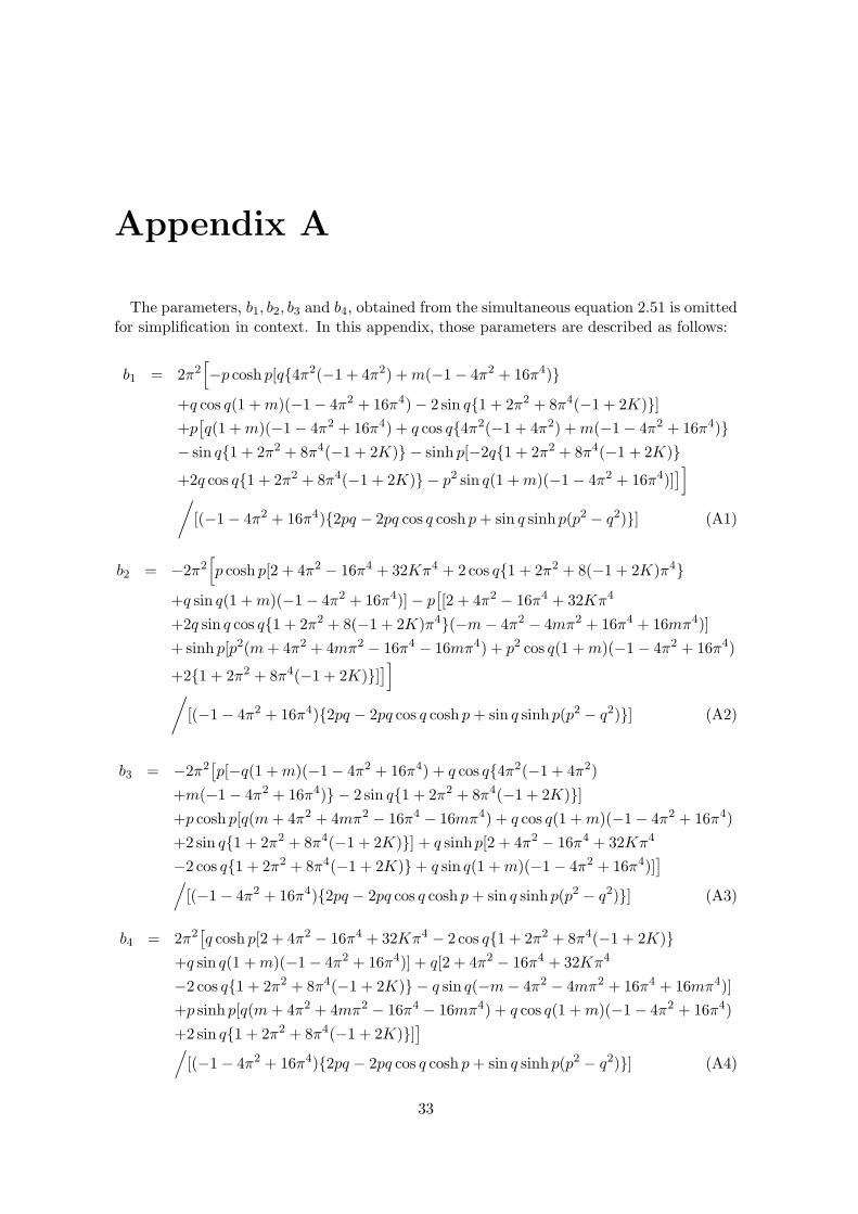
Appendix A

The parameters, b1, b2, b3 and b4, obtained from the simultaneous equation 2.51 is omittedfor simplification in context. In this appendix, those parameters are described as follows:

b1 = 2π2[−p cosh p[q{4π2(−1 + 4π2) + m(−1 − 4π2 + 16π4)}

+q cos q(1 + m)(−1 − 4π2 + 16π4) − 2 sin q{1 + 2π2 + 8π4(−1 + 2K)}]+p

[q(1 + m)(−1 − 4π2 + 16π4) + q cos q{4π2(−1 + 4π2) + m(−1 − 4π2 + 16π4)}

− sin q{1 + 2π2 + 8π4(−1 + 2K)} − sinh p[−2q{1 + 2π2 + 8π4(−1 + 2K)}+2q cos q{1 + 2π2 + 8π4(−1 + 2K)} − p2 sin q(1 + m)(−1 − 4π2 + 16π4)]

]]/

[(−1 − 4π2 + 16π4){2pq − 2pq cos q cosh p + sin q sinh p(p2 − q2)}] (A1)

b2 = −2π2[p cosh p[2 + 4π2 − 16π4 + 32Kπ4 + 2cos q{1 + 2π2 + 8(−1 + 2K)π4}

+q sin q(1 + m)(−1 − 4π2 + 16π4)] − p[[2 + 4π2 − 16π4 + 32Kπ4

+2q sin q cos q{1 + 2π2 + 8(−1 + 2K)π4}(−m − 4π2 − 4mπ2 + 16π4 + 16mπ4)]+ sinh p[p2(m + 4π2 + 4mπ2 − 16π4 − 16mπ4) + p2 cos q(1 + m)(−1 − 4π2 + 16π4)

+2{1 + 2π2 + 8π4(−1 + 2K)}]]]/[(−1 − 4π2 + 16π4){2pq − 2pq cos q cosh p + sin q sinh p(p2 − q2)}] (A2)

b3 = −2π2[p[−q(1 + m)(−1 − 4π2 + 16π4) + q cos q{4π2(−1 + 4π2)

+m(−1 − 4π2 + 16π4)} − 2 sin q{1 + 2π2 + 8π4(−1 + 2K)}]+p cosh p[q(m + 4π2 + 4mπ2 − 16π4 − 16mπ4) + q cos q(1 + m)(−1 − 4π2 + 16π4)+2 sin q{1 + 2π2 + 8π4(−1 + 2K)}] + q sinh p[2 + 4π2 − 16π4 + 32Kπ4

−2 cos q{1 + 2π2 + 8π4(−1 + 2K)} + q sin q(1 + m)(−1 − 4π2 + 16π4)]]

/[(−1 − 4π2 + 16π4){2pq − 2pq cos q cosh p + sin q sinh p(p2 − q2)}] (A3)

b4 = 2π2[q cosh p[2 + 4π2 − 16π4 + 32Kπ4 − 2 cos q{1 + 2π2 + 8π4(−1 + 2K)}

+q sin q(1 + m)(−1 − 4π2 + 16π4)] + q[2 + 4π2 − 16π4 + 32Kπ4

−2 cos q{1 + 2π2 + 8π4(−1 + 2K)} − q sin q(−m − 4π2 − 4mπ2 + 16π4 + 16mπ4)]+p sinh p[q(m + 4π2 + 4mπ2 − 16π4 − 16mπ4) + q cos q(1 + m)(−1 − 4π2 + 16π4)+2 sin q{1 + 2π2 + 8π4(−1 + 2K)}]]/

[(−1 − 4π2 + 16π4){2pq − 2pq cos q cosh p + sin q sinh p(p2 − q2)}] (A4)

33

Appendix B

We also experimentally investigate the effect of excitation on a simply supported buckledbeam. The experimental setup is shown in Figure B1. The difference between the appa-ratuses of the simply supported and clamped-clamped beams is only the supported points.The beam we show in this appendix is simply supported at the both ends by radial bearingsas shown in Figure B2. The radial bearings have slight Coulomb friction in circumferentialdirection.

FFT analyzer

Sensor

Slide bearing

Displacementsensor 2

Beam

Function generator

Power amplifier

Shaker

amplifier

Slidebearing

Displacementsensor 1

Linear motor

DC/CC power supply

SensorCurrent

This part is excited

Radial bearing

Figure B1: Experimental setup of the simply supported beam

First, we show in Figure B3 the equilibrium region of the deflection of the beam againstthe axial compressive force when the system is not excited. The symbol of © denotes theboundary of the steady state. At any points on the lines connecting the symbol ©, thebeam can remain at rest[8] at the initial deflection due to Coulomb friction. In the casewithout excitation, the steady state has the width, i.e., an infinite number of fixed points.

Next, we show the steady state of the deflection when the system is excited with fre-quencies of 30 Hz and 20 Hz in Figs. 4.4(a) and 4.4(b), respectively. In this figure, �represents the plot in the quasistationary forward sweep of P . The symbol of � stands for

34

Radial bearingBeam

Figure B2: Radial bearing of supporting point of beam

-40

-20

0

20

40

2.32.22.12.01.91.8

P [N]

v [m

m]

Figure B3: equilibrium region of the deflection of the beam v against the axial compressiveforce P without excitation

35

the quasistationary backward sweep of P from the upper right endpoint. The symbol of� stands for the quasistationary backward sweep of P from the lower right endpoint. Weobserve hysteresis as in the case of fixed-fixed beam.

In the case with excitation, the steady state has three equilibrium point at most.

We experimentally clarify that hysteresis occurs at a simply supported beam with exci-tation and the effect of Coulomb friction is canceled out by the excitation.

40

20

0

-20

-40

2.42.32.22.12.01.91.8

P [N]

v [m

m]

(a) Excitation frequency = 30 Hz, Amplitude of exci-tation = 0.17 mm

40

20

0

-20

-40

2.32.22.12.01.91.8

P [N]

v [m

m]

(b) Excitation frequency = 20 Hz, Amplitude of exci-tation = 0.17 mm

Figure B4: Relationship between deflection of the beam v and axial compressive force Punder the excitation

36