183

STABILITY TESTS ON A NUMERICAL SOLUTION OF APSEUDO-ACOUSTIC TTI WAVE EQUATION

M. Voegele, E. Tessmer, and D. Gajewski

email: martin.voegele@zmaw.dekeywords: TTI, modelling, pseudo-acoustic

ABSTRACT

In this work, the performance of two coupled second-order pseudo-acoustic differential equationswere tested on various 2D TTI macro-models. At this, we examined particularly the relation betweenartificially varied amounts of shear-wave velocity and the stability of the modelling. Moreover, theeffect of smoothing the underlying macro-model was studied. Contrary to expectations, reducingparameter contrasts may have a positive effect for simple models in a weakly anisotropic environ-ment but turns out to become counter-productive in more complex models or models with strongeranisotropy.Based on our investigations, we conclude that models with a rapid varying tilt of the symmetry axisand an increased number of interfaces favour the activation of non-physical, with propagation timegrowing solutions for pseudo-acoustic wave equations using the differential operators presented.

INTRODUCTION

The need for efficient and robust algorithms which take anisotropy into account, leads to a pseudo-acousticapproach which can be derived from the P-SV dispersion relation for the full-elastic system (Alkhalifah,1998). Unfortunately, modifying this relation by setting the amount of shear-wave velocity along the axisof symmetry artificially to zero not only simplifies qP-wave modelling but also enhances the model resultsto become susceptible to numerical instabilities in tilted transversely isotropic (TTI) media. This is the casefor numerous so far presented pseudo-acoustic wave equations (e.g Zhou et al. (2006); Du et al. (2008);Duveneck et al. (2008)). Especially in acoustic media with a varying tilt of the symmetry axis relative tothe coordinate system, all of them turned out to produce unphysical solutions for the wave equation whichdistort the modelling even after a few iteration steps (Bube et al., 2012). Coming from the conjecture thatzero shear velocities normal to the symmetry plane cause numerical instability, Fletcher et al. (2009) ad-vertised a new finite shear-wave velocity attempt which turned out to become numerically unstable as wellin TTI media.Based on their approach, we examine the performance of the two coupled second-order differential equa-tions (PDEs). The main purpose of these studies is to get a better idea of how to stabilise and (at best)prevent the activation of non-physical solutions of the wave equation in a TTI environment.

DERIVATION OF THE PSEUDO-ACOUSTIC WAVE EQUATION

The pseudo-acoustic wave equation is based on the dispersion relation of the three wave modes P, SVand SH which are obtained when solving the Christoffel equation for its eigenvalues and associatedeigenvectors.

184 Annual WIT report 2013

Since the SH-mode is decoupled, the P-SV dispersion relation for the phase velocities in the gen-eral 3D case is given by

ω4 = [(V 2px + V 2

sz)(k̂2x + k̂2

y) + (V 2pz + V 2

sz)k̂2z ]ω2 − V 2

pxV2sz(k̂

2x + k̂2

y)2

−V 2pzV

2sz k̂

4z + [V 2

pz(V2pn − V 2

px)− V 2sz(V

2pn − V 2

pz)] · (k̂2x + k̂2

y)k2z ,

(1)

where ω is the angular frequency, Vpz and Vsz are the P and S-wave velocities parallel to the symmetryaxis and Vpn = Vpz

√1 + 2δ is defined as the normal moveout velocity (Fletcher et al., 2009). The quantity

Vpx = Vpz√

1 + 2ε denotes the P-wave velocity parallel to the symmetry plane. By setting Vsz = 0, thedispersion relation corresponds to the approximation from which the first pseudo-acoustic wave equationwas derived by Alkhalifah (1998). The parameters k̂x, k̂y and k̂z are rotated wavenumbers with respect tothe symmetry axis in TI media.The solution for equation 1 is given by one fourth order or two coupled second-order partial differentialequations in time that are obtained by substituting the expression for the wave numbers from equation4 into the dispersion relation 1 and multiplying both sides with the pressure wave field p(ω, kx, ky, kz).Then, an inverse Fourier transform to both sides leads to the final equations presented by Fletcher et al.(2009)

∂2p

∂t2= V 2

pxH2p+ αV 2pzH1q + V 2

szH1(p− αq) + S

∂2q

∂t2=V 2pn

αH2p+ V 2

pzH1q − V 2szH2

(1

αp− q

)+ S . (2)

Here, q(ω, kx, ky, kz) denotes an auxiliary wave field and α = 1 is a non-zero scaling factor. In thedegenerated isotropic case, wave field p(ω, kx, ky, kz) equals q(ω, kx, ky, kz) and both PDEs from 2 areidentical. The variable S represents the source function and H1 and H2 are two introduced differentialoperators that contain single and mixed-space derivatives (for more details see appendix A).Since the numerical studies are performed in the two-dimensional x-z-domain, all derivatives with respectto the y-direction are zero. For the sake of minimising computational resources, spatial derivatives inequation 2 are solved using a pseudo-spectral algorithm introduced by Kosloff and Baysal (1982). Thetime integration is approximated using fourth-order Taylor expansions.

NUMERICAL STUDIES

The stability of the wave equation has been studied exemplary for the two-dimensional case on 105 syn-thetic anisotropic models ranging from homogeneous VTI models to more complex geological structureswith strong anisotropy and a rapid varying tilt angle θ. The reason for this large number of experiments isto find a common thread in

(a) the parametrisation of the anisotropy

(b) the complexity of the geology

of the models that are likely to end in numerical instability.We tested each model with 14 different shear-wave velocities, in order to point out their effect on themodelling. In addition to that, we investigated whether smoothing the underlying macro-model can beused to preserve stability. For this report, three subsurface models have been chosen representatively ofwhich the studies will be demonstrated in detail.

Annual WIT report 2013 185

Table 1: Parameters of representative macro-modelsε δ θ

Model 1 0.1 0.01 60◦

Model 2 0.11 -0.035 40◦

Model 3 0.15 0.081 0◦, 31◦, 51◦, 60◦

Model 1 and model 2 are two-layered models with an isotropic top layer with Vpz = 3000 m s−1 and asubjacent weakly TTI layer. The lower layer of model 2 resembles a Taylor sandstone where the parametersare taken from Thomsen (1986). Model 3 represents a geologically more complex anisotropic structurewith an overhang in an isotropic environment. It is based on a model from Fletcher et al. (2009) and ischaracterised by velocity contrasts between 2740 and 6000 m s−1 and strong variations in the tilt axisbetween 0◦ and 60◦.Apart from the Thomsen parameters that define the anisotropy in the models, a fourth parameter σ isintroduced to describe the kinematics of SV-waves (e.g. Tsvankin, 2001):

σ ≡(VpzVsz

)2

(ε− δ). (3)

The value of σ has been chosen in the range of 0.2 - 6 for each model. For σ → ∞, the SV-velocities inthe model become zero. Unfortunately, strong diamond-shaped shear-wave artefacts may impair the imageand the ratio Vpz/Vsz becomes physically unrealistic (Fletcher et al., 2009). For σ → 0, triplications in theSV-wave front disappear in strong anisotropic media. However, in this case the shear-wave velocities maybecome unphysically large.

RESULTS

General stability issue

Presenting the global maximum pressure amplitude over time for the example cases illustrates thewell-known stability issue of the pseudo-acoustic wave equation.Figure 1a) shows the global pressure trend of a wave field propagating in the weakly anisotropic two-layered model 1 with varying shear-wave velocities governed by σ. Despite a strong vertical variation ofthe tilt angle θ at the boundary layer, wave propagation can be considered as stable over time.Figure 1b) presents the trend of the global maximum pressure for model 2 in a weakly anisotropic envi-ronment of a Taylor sandstone. At first glance, the result for the propagating wave field remains relativelyconstant for all values of σ. However, after roughly 12000 iteration steps, the pressure amplitudes of all σvalues except σ = 0.2 start to grow.In contrast, the pressure trend of the geologically more complex model 3 is presented in figure 1c). Here,the pressure amplitudes of the propagating wave fields become unstable after roughly 3100 iteration steps.At this point, wave fields with smaller shear-wave velocities tend to become unstable more easily. By com-paring the gradient of the amplitude trends, one can recognise a slightly steeper slope for larger values of σ.

Combined with findings obtained from other test runs, the connection between parametrisation, numberof boundaries in the geology and unstable model results over time turn out to be very complex. Therefore,a direct determination of whether a subsurface configuration is suitable for modelling or not is impossible.Consequently the performance of smoothing is tested to reduce parameter contrasts in the model and delayinstabilities occurring during modelling.

186 Annual WIT report 2013

Figure 1: Global maximum pressure over time for (a) model 1 with a weakly anisotropic layer, (b) model2 with a subjacent weakly anisotropic Taylor sandstone layer and (c) model 3 with a variable tilt angle forvarying values of σ. The amplitudes are scaled logarithmically.

Smoothed macro-models

Fletcher et al. (2009) hints at rapid alterations of the orientation of the symmetry plane as the originof numerical instabilities in the model. For the numerical studies, the macro-models were smoothediteratively with a weighted two-dimensional window of second order. The intensity of smoothing has beencontrolled by applying the smoothing operator repeatedly to the model. For smoothing seismic velocities,the filter is applied on their slowness in order to preserve time-depth relations. The tilt angle distributionis smoothed without inversion. The result leads to smaller amplitude contrasts at the cost of decreasingspatial resolution of the structures in the model. Fortunately, not too strong smoothing the macro-modeldoes not necessarily lead to inaccurate migration results using pre-stack RTM (Tessmer, 2003).

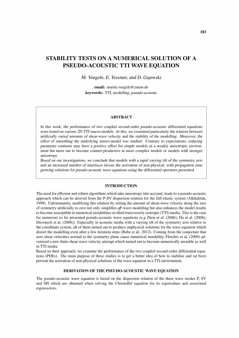
Figure 2 illustrates the results of applying the smoothing operator a) zero times, b) 500 times and c)1000 times on the weakly anisotropic macro-model 2 which will serve as an example in this section.Smoothing introduces spatial parameter changes to the macro-model. As a result, the formerly stablenumerical computations for a wave field in model 1 becomes highly unstable in figure 2b) 500 smoothingiterations and figure c) 1000 iterations. Whereas the activation of exponentially growing solutions for thePDEs arise shortly after 4000 time steps in the former case, doubling the application of the smoothingoperator not only reduces the contrasts in the macro-model stronger, but also delays exponentially growingpressure amplitudes. Again, higher values of σ advance the activation of numerical instabilities.

Annual WIT report 2013 187

Figure 2: Outcome of smoothing the weakly anisotropic model 1 with a different number of iterations: (a)no smoothing, (b) 500 smoothing iterations and (c) 1000 smoothing iterations. The amplitudes are scaledlogarithmically.

188 Annual WIT report 2013

CONCLUSIONS

In this report a pseudo-acoustic wave equation was tested in TTI media. The first part of the numericalstudies considered the performance of the algorithm in 105 two-dimensional macro-models that have beendefined through anisotropic parameters, the tilt angle of the symmetry axis, the vertical P-wave velocityand their geometries. Each model has hereby been tested with 14 different shear-wave velocities which arecontrolled by the parameter σ.Since each parameter value and its associated distribution alters the model results, the formerly stabilityissue which has been linked with zero shear-wave velocities turns out to be associated additionally withthe amount of anisotropy and the number of interfaces in the model. Consequently, the complexity ofthe model geometries was limited to the homogeneous, two-layered and multi-layered case in order tofacilitate the interpretation of the results.By trying to find a common thread within the parametrisation of the models, their geometry and therespective robustness of the model solutions, it is striking that increasing the number of interfaces within amodel while the anisotropic parameters are kept constant advances the activation of numerical instabilities.Vice versa, the degree of anisotropy amplifies occurring non-physical solutions of the PDE. Larger valuesfor σ lead to a stronger activation of instabilities.

Fletcher et al. (2009) stated in their work, that rapid variations in the tilt angle of the symmetry axisfavour numerical instability. This is in accordance with our findings since smoothing the model (andthus increasing the number of interfaces and parameter variations in the model) impairs the computationstremendously. In the case of TTI models with a high number of variations in the tilt axis and moderate tostrong anisotropy, the pressure amplitudes are likely to end in floating-point exceptions within few timesteps. Coming from the conjecture that an increased number of interfaces in the model compromises therobustness of the algorithm, it is understandable that smoothing is counter-productive.

Contrary to the conclusions of Fletcher et al. (2009), our studies reveal that even for non-zero shear-wave velocities, long propagation times lead to instability. As opposed to Bube et al. (2012) and Fletcheret al. (2009) who suggested that zero shear-wave velocities are the reason for numerical instabilities, wesuggest that time-growing solutions for the wave equation are likely to be inherent to the PDEs and resultfrom the implementation of the rotated differential operators (Zhang et al., 2011) (see appendix A).

PUBLICATIONS

More information on this work is presented in the Bachelor’s thesis of Voegele (2013).

ACKNOWLEDGMENTS

This work was kindly supported by the sponsors of the Wave Inversion Technology (WIT) Consortium,Karlsruhe, Germany. Especially we want to thank TEEC for the close cooperation in this work.

REFERENCES

Alkhalifah, T. (1998). Acoustic approximations for processing in transversly isotropic media. Geophysics,63(2).

Bube, K. P., Nemeth, T., Stefani, J. P., Ergas, R., Liu, W., Nihei, K. T., and Zhang, L. (2012). On thestability in second-order systems for acoustic VTI and TTI media. Geophysics, 77(5).

Du, X., Fletcher, R. P., and Fowler, P. J. (2008). A new pseudo-acoustic wave equation for VTI media:70th Annual Conference and Exhibition. EAGE, Expanded Abstracts, H033.

Duveneck, E., Bakker, P. M., and Perkins, C. (2008). Acoustic VTI wave equations and their applicationfor anisotropic reverse-time migration. 78th Annual International Meeting, SEG, Expanded Abstracts,2186-2190.

Fletcher, R. P., Du, X., and Fowler, P. J. (2009). Reverse time migration on tilted transversely isotropic(TTI) media. Geophysics, 74(6).

Annual WIT report 2013 189

Kosloff, D. D. and Baysal, E. (1982). Forward modeling by a Fourier method. Geophysics, 47.

Tessmer, E. (2003). Full-Wave Pre-Stack Reverse-Time Migration by the Fourier Method and Comparisonswith Kirchhoff Depth Migration. Annual WIT report.

Thomsen, L. (1986). Weak elastic anisotropy. Geophysics, 51(10).

Tsvankin, I. (2001). Seismic Signatures and Analysis of Reflection Data in Anisotropic Media, volume 29.Pergamon.

Voegele, M. (2013). Stability tests on a numerical solution of a pseudo-acoustic TTI wave equation. Uni-versität Hamburg. Bachelor Thesis.

Zhang, Y., Zhang, H., and Zhang, G. (2011). A stable TTI reverse time migration and its implementation.Geophysics, 76(3).

Zhou, H., Zhang, G., and Bloor, R. (2006). An anisotropic acoustic wave equation for modeling andmigration in 2D TTI media. 76th Annual International Meeting, SEG, Expanded Abstracts, pages 194–198.

APPENDIX A

ADDITIONAL INFORMATION ON THE PSEUDO-ACOUSTIC WAVE EQUATION

Since the P-SV dispersion relation 1 takes TTI media into account, two angles θ and φ are adopted in thedefinition of the wave numbers k̂x, k̂y and k̂z in the rotated system.

k̂x = kx cos θ cosφ+ ky cos θ sinφ− kz sin θ ,

k̂y = −kz sinφ+ ky cosφ,

k̂z = kx sin θ cosφ+ ky sin θ sinφ+ kz cos θ(4)

Here, θ is the tilt angle of the symmetry plane relative to the vertical axis of the coordinates and φ is theazimuth of the symmetry axis.

The two introduced differential operators H1 and H2 are given by:

H1 = sin2 θ cos2 φ∂2

∂x2+ sin2 θ sin2 φ

∂2

∂y2+ cos2 θ

∂2

∂z2+ sin2 θ sin 2φ

∂2

∂x∂z

+ sin 2θ sinφ∂2

∂x∂y+ sin 2θ cosφ

∂2

∂x∂y,

H2 =∂2

∂x2+

∂2

∂y2+

∂2

∂z2−H1 .

(5)