Stability and spectral convergence of Fourier method for …€¦ · Stability and spectral...

Numer. Math. (2015) 129:749–782DOI 10.1007/s00211-014-0652-y

NumerischeMathematik

Stability and spectral convergence of Fourier methodfor nonlinear problems: on the shortcomingsof the 2/3 de-aliasing method

Claude Bardos · Eitan Tadmor

Received: 24 August 2013 / Revised: 11 May 2014 / Published online: 15 July 2014© Springer-Verlag Berlin Heidelberg 2014

Abstract The high-order accuracy of Fourier method makes it the method of choicein many large scale simulations. We discuss here the stability of Fourier method fornonlinear evolution problems, focusing on the two prototypical cases of the inviscidBurgers’ equation and the multi-dimensional incompressible Euler equations. TheFourier method for such problems with quadratic nonlinearities comes in two mainflavors. One is the spectral Fourier method. The other is the 2/3 pseudo-spectralFourier method, where one removes the highest 1/3 portion of the spectrum; this isoften the method of choice to maintain the balance of quadratic energy and avoidaliasing errors. Two main themes are discussed in this paper. First, we prove that aslong as the underlying exact solution has a minimal C1+α spatial regularity, then boththe spectral and the 2/3 pseudo-spectral Fourier methods are stable. Consequently, weprove their spectral convergence for smooth solutions of the inviscid Burgers equationand the incompressible Euler equations. On the other hand, we prove that after acritical time at which the underlying solution lacks sufficient smoothness, then boththe spectral and the 2/3 pseudo-spectral Fourier methods exhibit nonlinear instabilitieswhich are realized through spurious oscillations. In particular, after shock formation ininviscid Burgers’ equation, the total variation of bounded (pseudo-) spectral Fouriersolutions must increase with the number of increasing modes and we stipulate theanalogous situation occurs with the 3D incompressible Euler equations: the limiting

C. BardosUniversity of Paris 7, Denis Diderot, Laboratory Jacques Louis Lions,University of Paris 6, Paris, Francee-mail: [email protected]

E. Tadmor (B)Department of Mathematics, Center of Scientific Computationand Mathematical Modeling (CSCAMM), Institute for Physical sciences and Technology (IPST),University of Maryland, College Park, MD 20742-4015, USAe-mail: [email protected]

123

750 C. Bardos, E. Tadmor

Fourier solution is shown to enforce L2-energy conservation, and the contrast withenergy dissipating Onsager solutions is reflected through spurious oscillations.

Mathematics Subject Classification (1991) 65M12 · 65M70 · 35L65 · 35Q31

Contents

1 Introduction . . . . . . . . . . . . . . . . . . . . . . . . . . . . . . . . . . . . . . . . . . . . 7501.1 Spectral convergence . . . . . . . . . . . . . . . . . . . . . . . . . . . . . . . . . . . . . 7521.2 Aliasing . . . . . . . . . . . . . . . . . . . . . . . . . . . . . . . . . . . . . . . . . . . . 753

2 Linear equations—lack of resolution and weak instability . . . . . . . . . . . . . . . . . . . . 7542.1 The 2/3 de-aliasing Fourier method and strong stability . . . . . . . . . . . . . . . . . . . 756

3 The 2/3 de-aliasing Fourier method for Burgers equation . . . . . . . . . . . . . . . . . . . . 7593.1 Stability and convergence for smooth solutions . . . . . . . . . . . . . . . . . . . . . . . . 7603.2 Instability for non-smooth solutions . . . . . . . . . . . . . . . . . . . . . . . . . . . . . 767

4 The 2/3 de-aliasing Fourier method for Euler equations . . . . . . . . . . . . . . . . . . . . . 7704.1 Convergence for smooth solutions . . . . . . . . . . . . . . . . . . . . . . . . . . . . . . 7704.2 Failure of convergence for weak solutions? . . . . . . . . . . . . . . . . . . . . . . . . . . 774

5 The spectral viscosity method: stability and spectral convergence . . . . . . . . . . . . . . . . 7766 Beyond quadratic nonlinearities: 1D isentropic equations . . . . . . . . . . . . . . . . . . . . . 779References . . . . . . . . . . . . . . . . . . . . . . . . . . . . . . . . . . . . . . . . . . . . . . . 781

1 Introduction

Spectral methods are often the methods of choice when high-resolution solvers aresought for nonlinear time-dependent problems. Here, we are concerned with the sta-bility and convergence of Fourier method for PDEs with quadratic nonlinearities: wefocus our attention on the prototypical Cauchy problems for the inviscid Burgers’equation and the incompressible Euler equations.

The Fourier methods for problems involving quadratic nonlinearities come in twomain flavors: the spectral Fourier method and the 2/3 smoothing of pseudo-spectralFourier method. The spectral Fourier method is realized in terms of N -degree Fourierexpansions, uN (x, t) = ∑|k|≤N uk(t)eik·x, where uk(t) are the Fourier moments ofu(x, t)

uk(t) = 1

(2π)d

∫

Td

u(x)e−ik·xdx, k := (k1, . . . , kd) ∈ Zd .

The computation of these moments in nonlinear problems is carried out by convo-lutions. These can be avoided when the uk’s are replaced by the discrete Fouriercoefficients, sampled at the (2N + 1)d equally spaced grid points

uk(t) =(

1

2N + 1

)d ∑

xν∈Td#

u(xν, t)e−ik·xν , xν = 2πν

2N + 1,

123

Stability and spectral convergence of Fourier method 751

where Td# is the discrete torus,

Td# :=

{

xν | xν = 2πν

2N + 1, ν = (ν1, . . . , νd), 0 ≤ ν j ≤ 2N

}

.

The pseudo-spectral Fourier method is realized in terms of the corresponding expan-sion, uN (x, t) =∑|k|≤N uk(t)eik·x. Here, we have the advantage that nonlinearitiesare computed as exact pointwise quantities at the grid points {xν}ν , but new aliasingerrors are introduced. To avoid aliasing errors and their potential instabilities, highmode smoothing is implemented, which results in the so-called 2/3-smoothing ofpseudo-spectral Fourier method: it is realized in terms of the 2N/3-degree expansion,uN (x, t) = ∑|k|≤2N/3 σkuk(t)eik·x. This is the spectral method of choice in manytime-dependent problems with quadratic nonlinearities.

To put our discussion into perspective we begin, in Sect. 2, by recalling the linearsetup of standard transport equation. The spectral Fourier method is L2-stable. But thepseudo-spectral Fourier method is not [14]: it is only weakly stable, due to amplificationof aliasing errors when the underlying solution lacks sufficient smoothness. Strong L2-stability is regained with the 2/3-smoothing of pseudo-spectral Fourier method [42];in the linear setup, the de-aliasing in the 2/3-method introduces sufficient smoothnessto maintain convergence. This is one of the main two themes of our results on nonlinearproblems: sufficient smoothness guarantees stability and hence spectral convergence.In Sect. 3 we explore this issue in the context of inviscid Burgers equations, provingthat as long as the solution of the inviscid Burgers equation remains smooth, u(·, t) ∈C1+α

x , then both the spectral and the 2/3-pseudo-spectral Fourier approximations,uN (·, t), converge to the exact solution. Moreover, they enjoy spectral convergencerate, namely, the convergence rate grows with the increasing smoothness of u(·, t),

∫

|uN (x, t)− u(x, t)|2dx

� e∫ t

0‖ux (·,τ )‖L∞ dτ·(

N−2s‖u(·, 0)‖2Hs + N

32 −s max

τ≤t‖u(·, τ )‖Hs

)

, s >3

2.

A similar statement of spectral convergence holds for the spectral and 2/3 pseudo-spectral Fourier approximations uN of the incompressible Euler equations: in Sect. 4we prove that as long as u(·, t) remains sufficiently smooth solution of the d-dimensional Euler equations, u(·, t) ∈ C1+α

x , then

‖uN (·, t)− u(·, t)‖2L2

� e2∫ t

0‖∇xu(·,τ )‖L∞ dτ·(

N−2s‖u(·, 0)‖2Hs +N

d2+1−s max


)

, s>d

2+1.

These results support the superiority of spectral methods for problems with smoothsolutions. When dealing with solutions which lack smoothness, however, both the spec-tral and 2/3 pseudo-spectral Fourier methods suffer nonlinear instabilities. This is theother main theme of the paper, explored in the context of the inviscid Burgers equation

123


and the incompressible Euler equations in the respective Sects. 3.2 and 4.2. In particu-lar, we prove that after shock formation, the spectral and 2/3 pseudo-spectral boundedapproximations of the inviscid Burgers solution must produce spurious oscillations astheir total variation must increase, ‖uN (·, t)‖T V � 4

√N . This is deduced by contra-

diction: in Theorem 3.4 below we prove, using compensated compactness arguments,that an L2-weak limit of slowly growing TV Fourier solutions, u = w lim uN , mustbe an L2-energy conservative solution, which cannot hold once shocks are formed.

A similar scenario arises with the Euler solutions where the spectral and the (2/3pseudo-)spectral approximations of Euler equations enforce conservation of the L2-energy. Although there is no known energy dissipation-based selection principle toidentify a unique solution of Euler equations within the class of “rough” data (similarto the entropy dissipation selection principle for Burgers’ equations), nevertheless weargue that the L2-energy conservation of the (pseudo-)spectral approximations may beresponsible to their unstable behavior. While L2-energy conservation holds for weaksolutions with a minimal degree of 1/3-order of smoothness (Onsager’s conjectureproved in [3,8,13]), there are experimental and numerical evidence for the other partof Onsager’s conjecture that anomalous dissipation of energy shows up for “physical-turbulent” L2-solutions of Euler equations [7]. Whether this observed anomalousdissipation of energy should be due to spontaneous appearance of singularities insmooth solutions of the Euler equation or to the fact that physical initial data may berough is a completely open problem. However after several preliminary breakthrough[37] and [39] the following fact are now well established. Indeed, there are infinitelymany initial data (which of course are not regular) leading to infinitely many weakEuler solutions with energy loss [10]. In particular there are energy decaying solutions

which for almost every time belong to the critical regularity C13 −ε [4]. Thus, if the

numerical method captures such “rough” solutions then the “unphysical” conservationof energy which is enforced at the spectral level has to vanish at the limit, leading tospurious oscillations.

The nonlinear instability results in Sects. 3.2 and 4.2 emphasize the competi-tion between spectral convergence for smooth solutions vs. instabilities for problemswhich lack sufficient smoothness due to their quadratic nonlinearities. We then closethis paper with two complementary results. First, in Sect. 5 we make a brief com-ments how these instabilities can be overcome using the class of spectral viscosity(SV) methods which entertain both—spectral convergence and nonlinear stability,[2,16,18,38,43,45]. This is achieved by adding a judicious amount of spectral viscos-ity at the high-portion of the spectrum without sacrificing the spectral accuracy at thelower portion of the spectrum. Finally, in we Sect. 6 we note that the above stabilityresult for smooth solutions of nonlinear equations go beyond quadratic nonlinearities,where we prove the stability of Fourier method for smooth solutions of the nonlinearisentropic equations.

1.1 Spectral convergence

Expressed in terms of the Fourier coefficients, w(k), the spectral Fourier projectionPN [w](x) of w ∈ L1[Td ] is given by

123


PN [w](x)=∑

|k|≤N

w(k)eik·x, w(k) := 1

(2π)d

∫

Td

w(x)e−ik·xdx, k := (k1, . . . , kd)∈Zd .

The convergence rate of the truncation error,

(I − PN )[w](x) :=∑

|k|≥N

w(k)eik·x, (1.1)

is as rapid as the global smoothness of w permits (and observe that the degree ofsmoothness is allowed to be negative),

‖(I − PN )[w]‖Hr ≤ Nr−s‖w‖H s , s>r ∈R;

in particular,

maxx

|(I − PN )[w](x)| � Nd2 −s‖w‖Hs , s >

d

2. (1.2)

These are statements of spectral convergence rate: the smoother w is, the faster isthe convergence rate of (I − PN )[w] → 0. In practice, one recovers exponentialconvergence which characterizes analytic regularity or at least root-exponential ratefor typical compactly supported Gevrey-regular data [48].

1.2 Aliasing

Set h := 2π2N+1 as a discrete spacing. If we replace the integrals with quadrature based

on sampling w at the (2N + 1)dequi-spaced points, xν := νh, ν := (ν1, . . . , νd) ∈{0, . . . , 2N }d , we obtain the pseudo-spectral Fourier projection,

ψN [w](x) =∑

|k|≤N

w(k)eik·x, w(k) :=(

h

2π

)d ∑

xν∈Td#

w(xν)e−ik·xν , |k| ≤ N .

Here, w(k), are the discrete Fourier coefficients.1 The mapping w → ψN [w] is aprojection: ψN [w](x) is the unique N -degree trigonometric interpolant of w at the(2N + 1)-gridpoints, ψN [w](xν) = w(xν), |ν| ≤ 2N . The dual statement of the lastequalities is the Poisson summation formula, which determines the discrete w(k)’s interms of the exact Fourier coefficients, w(k)’s,

w(k) = w(k)+∑

� �=0

w(k + �(2N + 1)), |k| ≤ N ,

1 There is a slight difference between the formulae based on an even and an odd number of points; wechose to continue with the slightly simpler notations associated with an odd number of points.

123


where summation runs over all d-tuples, � = (1, . . . , d) �= 0. It shows that all theFourier coefficients with wavenumber k[mod(2N + 1)] are “aliased” into the samediscrete Fourier coefficient, wk. It follows that the interpolation error consists of twomain contributions,

(I − ψN )[w] ≡ (I − PN )[w] + AN [w],

where in addition to the truncation error (I −PN )[w] in (1.1), we now have the aliasingerror,

AN [w](x) :=∑

|k|≤N

⎛

⎝∑

|�|≥1

w(k + �(2N + 1))

⎞

⎠ eik·x. (1.3)

Both, (I − PN )[w] and AN [w], involve high modes, w(p), |p| ≥ N . Consequently,if the function w(·) is sufficiently smooth then they have exactly the same spectrallysmall size, e.g. [46, §2.2]

‖AN [w]‖Hs � ‖(I − PN )[w]‖Hs � N s−r‖w‖Hr , r > s >d

2.

The situation is different, however, if w lacks smoothness. Since the truncation erroris orthogonal to the computational N-space whereas the aliasing error is not, aliasingand truncation errors may have a completely different influence on the question ofcomputational stability. One such case is encountered with the stability question ofspectral vs. pseudo-spectral approximations of hyperbolic equations.

2 Linear equations—lack of resolution and weak instability

We begin with the spectral Fourier method. We want to solve the 2π -periodic scalarhyperbolic equation

∂

∂tu(x, t)+ ∂

∂x(q(x)u(x, t)) = 0, x ∈ T([0, 2π)), q ∈ C1[0, 2π ], (2.1)

subject to prescribed initial conditions, u(·, 0), by the spectral method. To this end weapproximate the spectral projection of the exact solution, PN u(·, t), using an N -degreepolynomial, uN (x, t) = ∑|k|≤N uk(t)eikx , which is governed by the semi-discreteapproximation [15,22,32]

∂

∂tuN (x, t)+ ∂

∂xPN [q(x)uN (x, t)] = 0. (2.2a)

The approximation is realized as a convolution in Fourier space

d

dtuk(t) = ik

∑

| j |≤N

q(k − j )u j (t), k = −N , . . . , N , (2.2b)

123


which amounts to a system of (2N + 1) ODEs for the computed u(t) :=(u−N (t), . . . , uN (t)) .

The L2-stability of (2.2a) is straightforward: though the truncation error whichenters (2.2a), ∂x (I − PN )[q(x)uN (x)] need not be small, it is orthogonal to the N -space, which yields the L2-stability bound, ‖uN (·, t)‖2

L2 ≤ eq ′∞t‖uN (·, 0)‖2L2 with

q ′∞ := maxx |q ′(x)|.To convert this stability bound into a spectral convergence rate estimate, consider the

difference between the spectral method (2.2a) and the PN projection of the underlyingequation (2.1): one finds that eN := uN − PN u, satisfies the error equation

∂

∂teN (x, t)+ ∂

∂xPN [q(x)eN (x, t)] = − ∂

∂xPN [q(x)(I − PN )[u](x, t)] .

The L2-stability bound of the spectral method implies the error estimate,

∫

|uN (x, t)− PN u(x, t)|2dx

� eq ′∞t(

‖(I − PN )u(·, 0)‖2L2 + N 2 max

τ≤t‖(I − PN )[u](·, τ )‖2

L2

)

.

This quantifies the spectral convergence of the Fourier method (2.2a): the convergencerate increases together with the increasing order of smoothness of the solution,

‖uN (·, t)− u(·, t)‖L2 �e12 q ′∞t(

N−s‖u(·, 0)‖Hs + N 1−s maxτ≤t

‖u(·, τ )‖Hs

)

, s>1.

(2.3)In practice, one recovers exponential convergence for analytic solutions (and root-exponential convergence for more general Gevrey data).

Next, we turn to consider the pseudo-spectral Fourier method of (2.1). Here, weavoid the need to compute convolutions as in (2.2b) at the expense of additionalaliasing errors which are responsible for weak stability. As before, we use an N -degree polynomial, uN (x, t) =∑|k|≤N uk(t)eikx , as an approximation for ψN u(·, t),which is governed by the semi-discrete approximation, [15,22],

∂

∂tuN (x, t)+ ∂

∂xψN [q(x)uN (x, t)] = 0. (2.4)

This equation can be realized in physical space

d

dtuN (x j , t) =

N∑

k=−N

ik (quN )keikx j , (quN )k = h

2π

2N∑

ν=0

q(xν)uN (xν)e−ikxν ,

which amounts to a system of (2N + 1) ODEs for the computed gridvalues u(t) :=(u(x0, t), . . . , u(x2N , t)) .

123


To examine the stability of (2.4) we repeat the usual L2-energy argument for thespectral approximation in (2.2a): decompose ψN = PN + AN , to find

1

2

d

dt‖uN (·, t)‖2

L2 =contribution of truncation

︷︸︸︷∫

uN∂

∂xPN [q(x)uN ]dx +

contribution of aliasing︷︸︸︷∫

uN∂

∂xAN [q(x)uN ]dx (2.5)

The first term on the right consists of truncation error which does not exceed12 q ′∞‖uN (·, t)‖2. Thus, the stability of the Fourier approximation (2.4) depends solelyon the aliasing contributions, AN [q(x)uN ]: using (1.3) to expand the second term onthe right, we find

∫

uN∂

∂xAN [q(x)uN ]dx = 2π i

∑

| j |,|k|≤N

u j (t )uk(t) ( j −k) ·∑

�=0

q ( j −k+(2N +1)) .

(2.6)

Observe that the terms on the right,∑ �=0 q( j − k + (2N + 1)), are of order O(N )

for | j − k| ∼ 2N , = ±1, and this can occur only for high wavenumbers, | j | ∼|k| ∼ N . Thus, there is possible O(N ) amplification of the high Fourier modes,|u j (t)|, | j | ∼ N . Unfortunately, these Fourier modes need not be small due to lackof a priori smoothness, and aliasing may render the Fourier method as unstable.

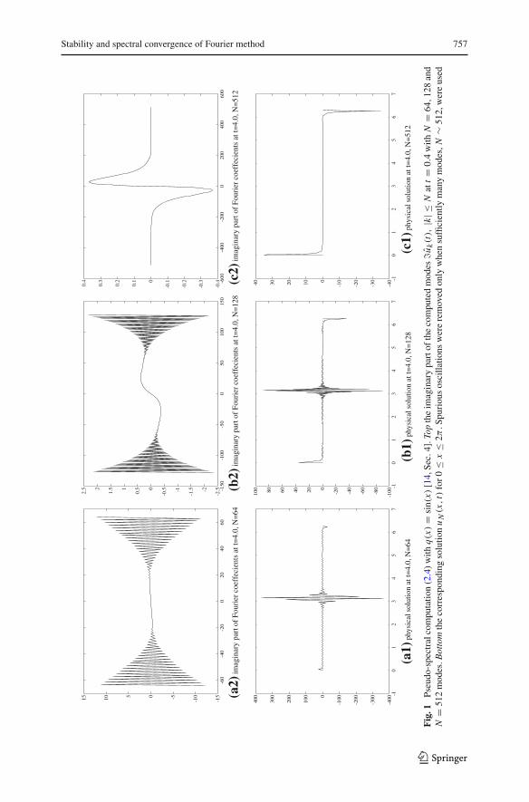
Indeed, we recall that even if the solution of (2.1) remains smooth, the exact solutionof (2.1) develops large gradients of order |u(t)| ∼ exp(q ′∞t)when q(x) changes sign,and consequently the Fourier method does experience spurious oscillations preciselybecause of amplification of aliasing errors. The detailed analysis carried out in [14]shows that these large gradients require N � et modes in order to be fully resolved;otherwise, the exact solution u(·, t) remains under-resolved by the pseudo-spectralFourier approximation. Without these many modes, the under-resolved Fourier approx-imation contains O(1) high modes which are amplified by a factor of order O(N ),yielding weak instability, noticeable as the spurious oscillations in Fig. 1. Thus, alias-ing errors cause the Fourier solution spurious O(N ) growth due to lack of resolution.The corresponding error estimate for the pseudo-spectral approximation reads [14,theorem 4.1]

‖uN (·, t)− ψN u(·, t)‖L2

� eCsq ′∞t(

N 1−s‖u(·, 0)‖Hs + N 2−s maxτ≤t

‖u(·, τ )‖Hs

)

, s > 2,

reflecting the loss of power on N when compared with the spectral estimate (2.3).

2.1 The 2/3 de-aliasing Fourier method and strong stability

One way to regain the stability of the pseudo-spectral Fourier method in (2.4) is to setthe highest pseudospectral modes in (2.4) u j (t) ≡ 0, | j | ∼ N . This prevents unstable

123


-15

-10-5051015

-60

-40

-20

020

4060

(a2)

imag

inar

y pa

rt o

f Fo

urie

r co

effe

cien

ts a

t t=

4.0,

N=

64

-2.5-2

-1.5-1

-0.50

0.51

1.52

2.5 -1

50-1

00-5

00

5010

015

0

(b2

) im

agin

ary

part

of

Four

ier

coef

feci

ents

at t

=4.

0, N

=12

8

-0.4

-0.3

-0.2

-0.10

0.1

0.2

0.3

0.4 -6

00-4

00-2

000

200

400

600

(c2)

imag

inar

y pa

rt o

f Fo

urie

r co

effe

cien

ts a

t t=

4.0,

N=

512

-400

-300

-200

-1000

100

200

300

400 -1

01

23

45

67

(a1)

phy

sica

l sol

utio

n at

t=4.

0, N

=64

-100-80

-60

-40

-20020406080100 -1

01

23

45

67

(b1)

phy

sica

l sol

utio

n at

t=4.

0, N

=12

8

-40

-30

-20

-10010203040

-10

12

34

56

7

(c1)

phy

sica

l sol

utio

n at

t=4.

0, N

=51

2

Fig

.1Ps

eudo

-spe

ctra

lcom

puta

tion

(2.4

)w

ithq(x)=

sin(

x)[1

4,Se

c.4]

.Top

the

imag

inar

ypa

rtof

the

com

pute

dm

odes

�uk(t),

|k|≤

Nat

t=

0.4

with

N=

64,12

8an

dN

=51

2m

odes

.Bot

tom

the

corr

espo

ndin

gso

lutio

nu

N(x,t)

for

0≤

x≤

2π.S

puri

ous

osci

llatio

nsw

ere

rem

oved

only

whe

nsu

ffici

ently

man

ym

odes

,N∼

512,

wer

eus

ed

123


growth due to aliasing. For example, assume that we truncate the last 1/3 of the modesof uN (any other fixed fraction of N will do). To this end, we use a smoothing operatorS which is activated only on the first 2

3 N modes while removing the top 1/3N of themodes. We up with the so-called 2/3 pseudo-spectral Fourier method,

∂

∂tuN (x, t)+ ∂

∂xψN [q(·)SuN ](x, t) = 0, SuN :=

∑

|k|≤ 23 N

σk uk(t)eikx ; (2.7a)

To retain spectral accuracy, the smoothing factors σk ∈ (0, 1] do not change a fixedportion of the lower spectrum

σk

⎧⎨

⎩

≡ 1, |k| ≤ 13 N

∈ (0, 1], 13 N < |k| < 2

3 N .(2.7b)

The L2-stability of the 2/3 method follows along the lines of [42, Sect. 6]. Indeed,the aliasing contribution in the 2/3 method corresponding to (2.6) amounts to

∫

(SuN )∂

∂xAN [q(·)(SuN )]dx = 2π i

∑

| j |≤ 23 N

∑

|k|≤ 23 N

σkσ j u j (t )uk(t) ( j − k)

·∑

�=0

q

| j−k+(2N+1)|≥ 23 N

︷︸︸︷( j − k + (2N + 1)) .

Observe that the terms involved in the inner summation on the right are now restrictedto high wavenumbers, | j − k + (2N + 1)| ≥ 2

3 N so that |q( j − k + (2N + 1))| �‖q‖Cr N−r . Hence

∣∣∣∣

∫

(SuN )∂

∂xAN [q(·)(SuN )]dx

∣∣∣∣ � ‖q‖Cr N 1−r × ‖SuN ‖2, r ≥ 1. (2.8)

Using (2.8) with r = 1 together with standard spectral bound we arrive at

1

2

d

dt

∫

(SuN )(x, t)uN (x, t)dx = −∫

(SuN )∂

∂x(PN + AN )[q(·)(SuN )]dx

≤ Cq ′∞‖SuN (·, t)‖2L2 .

Thus, by activating the smoothing operator we removed aliasing errors and the resulting2/3 de-aliased pseudo-spectral method (2.7) regained the weighted L2-stability

‖uN (·, t)‖2L2

S≤ e2Cq ′∞t‖uN (·, 0)‖2

L2S,

‖w(·, t)‖2L2

S:=∫

(Sw)(x, t)w(x, t)dx ≡ 2π∑

|k|≤ 23 N

σk |wk(t)|2.

123


The corresponding error equation for eN := SuN − Su reads (we skip the details)

∂

∂teN + ∂

∂x(S[qeN ]) = − ∂

∂xS [q(x)(I − S)[u](x, t)] ,

and the spectral convergence rate (2.3), follows: for s > 1 there exists a constant,C = Cs such that

‖uN − u‖L2S

� eCsq ′∞t(

N−s‖u(·, 0)‖Hs + N 1−s maxτ≤t

‖u(·, τ )‖Hs

)

, s > 1.

Remark 2.1 (Spectral accuracy and propagation of discontinuities) Hyperbolic equa-tions propagates Hs regularity: ‖u(·, t)‖Hs � eCs t‖u(·, 0)‖Hs < ∞. Thus, theconvergence statement in (2.3) implies spectral convergence of the spectral Fouriermethod and 2/3 Fourier method for Hs-smooth initial data. However, when the ini-tial data is piecewise smooth, the exact solution propagates discontinuities alongcharacteristics, and the (pseudo-)spectral approximations of jump discontinuitiesin u(·, t) produces spurious Gibbs oscillations [48]. Nevertheless, thanks to theHs-stability of the spectral Fourier method and the 2/3 pseudo-spectral methods,‖uN (·, t)‖H s � eCs |q|∞t‖uN (·, 0)‖H s , measured in the weak topology of s < 0, the(pseudo-)spectral approximations still propagate accurate information of the smoothportions of the exact solution. This is realized in terms of the convergence rate (weskip the details)

‖uN − u‖Hr

� eCsq ′∞t(

Nr−s‖u(·, 0)‖Hs + N 1+r−s maxτ≤t

‖u(·, τ )‖Hs

)

, r < s − 1 < −1.

It follows that one can pre- and post-process uN (·, t) to recover the pointvalues ofu(·, t) within spectral accuracy, away from the singular set of the solution, [1,26,27].The point to note here is that although the Fourier projections of the exact solution,PN u(·, t) and ψN u(·, t) are at most first-order accurate due to Gibbs oscillations, thepost-processing of the computed uN which is realized by its smoothing using a properσ -mollifier (2.7b) (or see (3.6c) below) does both—retains the stability and recoversthe spectrally accurate resolution content of the Fourier method.

3 The 2/3 de-aliasing Fourier method for Burgers equation

We now turn our attention to spectral and pseudo-spectral approximations of non-linear problems. Their spectral accuracy often make them the method of choice forsimulations where the highest resolution is sought for a given number of degrees offreedom. We begin with the prototypical example for quadratic nonlinearities, theinviscid Bugers’ equation,

∂

∂tu(x, t)+ 1

2

∂

∂xu2(x, t) = 0, x ∈ T([0, 2π)), (3.1)

123


subject to 2π -periodic boundary conditions and prescribed initial conditions, u(x, 0).In this section we show that as long as the solution of Burgers equation remainssmooth for a time interval t ≤ Tc, the spectral and 2/3 de-aliased pseudo-spectralapproximations converge to the exact solution with spectral accuracy.

3.1 Stability and convergence for smooth solutions

We begin with the spectral approximation of (3.1), uN (x, t) =∑ uk(t)eikx , which isgoverned by,

∂

∂tuN (x, t)+ 1

2

∂

∂x

(PN

[u2

N

](x, t)

)= 0, 0 ≤ x ≤ 2π. (3.2)

The evaluation of the quadratic term on the right is carried out using convolu-tion and (3.2) amounts to a nonlinear system of (2N + 1) ODEs for u(t) =(u−N (t), . . . , uN (t)) .

Theorem 3.1 (Spectral convergence for smooth solutions of Burgers’ equations).Assume that for 0 < t ≤ Tc, the solution of the Burgers equation (2.1) is smooth,u(·, t) ∈ L∞([0, Tc],C1+α(0, 2π ]). Then, the spectral method (3.2) converges inL∞([0, Tc], L2(0, 2π ]),

‖uN (·, t)− u(·, t)‖L2 → 0, 0 ≤ t ≤ Tc.

Moreover, the following spectral convergence rate estimate holds for all s > 32 ,

‖uN (·, t)− u(·, t)‖2L2

� e∫ t

0|ux (·,τ )|∞dτ(

N−2s‖u(·, 0)‖2Hs + N

32 −s max


)

, s >3

2.

Proof We rewrite the spectral approximation (3.1) in the form

∂

∂tuN + ∂

∂x

u2N

2= 1

2

∂

∂x(I − PN )[u2

N ].

The corresponding energy equation reads

∂

∂t

u2N

2+ ∂

∂x

u3N

6= uN

2

∂

∂x(I − PN )[u2

N ]. (3.3)

Integration yields the energy balance

1

2

d

dt

∫

u2N (x, t)dx = 1

2

∫

uN ∂x (I − PN )[u2N ]dx =: I1.

123


The term on the right vanishes by orthogonality, I1 = − 12

∫∂uN∂x (I − PN )[u2

N ]dx = 0,and hence the solution is L2-conservative,

‖uN (·, t)‖L2 = ‖uN (·, 0)‖L2 . (3.4)

Next, we integrate (uN − u)2 ≡ |uN |2 − |u|2 − 2u(uN − u): after discarding allterms which are in divergence form, we are left with

1

2

d

dt

∫

(uN −u)2dx = d

dt

∫ ( |uN |22

− |u|22

−u(uN − u)

)

dx

= 1

2

∫

uN ∂x (I −PN )[u2N ]dx−

∫

∂t (u(uN −u))dx =: I1+I2.

Recall that I1 vanishes. As for the second term I2, we decompose it into two terms,

I2 =∫

∂t (u(uN − u)) dx ≡∫

ut (uN − u)dx +∫

u(∂t uN − ∂t u)dx,

and using (3.1), (3.2) and (3.3) to convert time derivatives to spatial ones, we find

I2 = −∫

uux (uN − u)dx −∫

u∂x

(u2

N

2− u2

2

)

dx + 1

2

∫

u∂x (I − PN )[u2N ]dx

= −∫

uux (uN − u)dx +∫

ux

(u2

N

2− u2

2

)

dx − 1

2

∫

ux (I − PN )[u2N ]dx

=∫

ux

(u2

N

2− u2

2− u(uN − u)

)

dx − 1

2

∫

ux (I − PN )[u2N ]dx .

Eventually, we end up with

1

2

d

dt

∫

|uN (x, t)− u(x, t)|2dx ≤ |ux (·, t)|L∞

2

∫

|uN (x, t)− u(x, t)|2dx − 1

2eN ,

(3.5a)where the error term, eN , is given by

eN :=∫

u2N (I − PN )[ux ]dx (3.5b)

Observe that under the hypothesis ux ∈ L∞t C0,α

x , and hence by Jackson’s bound [11]and the L2-bound (3.4) one has

|eN (t)| � maxx

|(I − PN )[ux (x, t)]| · ‖uN ‖2L2 � ln N

Nα‖uN (·, 0)‖2

L2 → 0.

123


With (3.5) one obtains,

∫

|uN (x, t)− u(x, t)|2dx ≤ eU ′∞(t;0)∫

|uN (x, 0)− u(x, 0)|2dx

+t∫

0

eU ′∞(t;τ)|eN (τ )|dτ, U ′∞(t; τ) :=t∫

s=τ|ux (·, s)|∞ds.

and convergence follows. Moreover, with uN (·, 0) = PN u(·, 0) we end up with spec-tral convergence rate estimate

∫

|uN (x, t)− u(x, t)|2dx

� e∫ t

0 |ux (·,τ )|∞dτ(

N−2s‖u(·, 0)‖2Hs + N

32 −s max


)

, s >3

2.

��Next, we turn to consider the pseudo-spectral approximation of Burgers equation

[15,22],

∂

∂tuN (x, t)+ 1

2

∂

∂x

(ψN

[u2

N

](x, t)

)= 0, x ∈ T([0, 2π)).

Observe that (3.1) is satisfied exactly at the gridpoints xν ,

d

dtuN (xν, t)+ 1

2

∂

∂x

(ψN

[u2

N

](x, t)

)∣∣x=xν

= 0, ν = 0, 1, . . . , 2N .

The resulting system of (2N + 1) nonlinear equations for u(t) = (u(x0, t), . . . ,u(x2N , t)) can be then integrated in time by standard ODE solvers. The pseudo-spectral approximation introduces aliasing errors which were shown to introduce weakinstability already in the linear case. To eliminate these errors, we consider the 2/3de-aliasing Fourier method, consult (2.7a)

∂

∂tuN (x, t)+ 1

2

∂

∂x

(ψN

[(SuN )

2](x, t)

)= 0, x ∈ T([0, 2π)), (3.6a)

where SuN denotes a smoothing operator of the form

SuN :=∑

|k|≤ 23 N

σk uk(t)eikx , uk(t) = h

2π

2N∑

ν=0

uN (xν, t)e−ikxν . (3.6b)

The smoothing operator S is dictated by the smoothing factors, {σk}|k|≤ 23 N , which

truncates modes with wavenumbers |k| > 23 N while leaving a fixed portion—say, the

first 1/3 of the spectrum, viscous-free. This is the same smoothing operator SuN we

123


considered already in the linear 2/3 method (2.7a). In typical cases, one may employa smoothing mollifier, σ(·) ∈ C∞(0, 1), setting

σk = σ

( |k|N

)

, σ (ξ)

⎧⎪⎪⎨

⎪⎪⎩

≡ 1, ξ ≤ 13 ,

∈ (0, 1), 13 < ξ < 2

3 ,

≡ 0, 23 ≤ ξ ≤ 1.

(3.6c)

This is the 2/3 de-aliasing Fourier method which is often advocated for spectralcomputations, in particular those involving quadratic nonlinearities [17,19,20,30].

In what sense does the 2/3 method remove aliasing errors? to make precise thede-aliasing aspect of (3.6), consider the 2/3 truncated solution um := SuN . Here weemphasize that we are dealing with the smoothed solution, um , of degree m := 2

3 N .Observing that truncation commute with differentiation, we find

∂

∂tum(x, t)+ 1

2

∂

∂xS(ψN [u2

m])(x, t) = 0, deg(um) = m := 2

3N . (3.7)

We now come to the key point behind the removal of aliasing in quadratic nonlin-earities: since um(k) = 0 for |k| > 2

3 N then u2m(k) = 0 for |k| > 4

3 N hence

u2m(k + (2N + 1)) = 0 for |k| ≤ 2

3 N , �= 0; consequently, since the smoothingoperator S acts only on the first 2

3 N mode, S(AN u2m) ≡ 0, and we conclude

S(ψN [u2

m])(x, ·) ≡ S

((PN + AN ) [u2

m])(x, ·)= S

(PN [u2

m])(x, ·) ≡ Su2

m(x, ·).

We summarize by stating the following.

Corollary 3.2 Consider the 2/3 de-aliasing Fourier method (3.6) then its 2/3smoothed solution, um := SuN , satisfies

∂

∂tum(x, t)+ 1

2

∂

∂xS[u2

m](x, t) = 0, Sw =∑

|k|≤m

σkwkeikx , m = 2

3N . (3.8)

Thus, by truncating the top 1/3 of the modes, we de-aliased the Fourier method (3.6a),in the sense that (3.8) does not involve any aliasing errors: only truncation errors,(I − S)[u2

m] are involved. Indeed, the formulation of 2/3 method in (3.8) resemblesthe m-mode spectral method (3.2). The only difference is due to the fact that unlessσk ≡ 1, the smoothing operator S is not a projection2

The following theorem shows that as long as the Burgers solution remains smooth,the 2/3 de-aliasing Fourier method is stable and enjoys spectral convergence.

2 When σk ≡ 1, then S = P23 N

and the 2/3 method coincides with the spectral Fourier method (3.2) with

m = 23 N modes,

∂

∂tum (x, t)+ 1

2

∂

∂xPm [u2

m ](x, t) = 0, |k| ≤ 2

3N .

123


Theorem 3.3 (Spectral convergence of the 2/3 method for smooth solutions). Assumethat for 0 < t ≤ Tc, the solution of the Burgers equation (2.1) is smooth,u(·, t) ∈ L∞([0, Tc],C1+α(0, 2π ]). Then, the 2/3 de-aliasing method (3.6) convergesin L∞([0, Tc], L2(0, 2π ]),

‖um(·, t)− u(·, t)‖L2 → 0, 0 ≤ t ≤ Tc,

and the following spectral convergence rate estimate holds

‖uN (·, t)− u(·, t)‖2L2

� e∫ t

0 |ux (·,τ )|∞dτ(

N−2s‖u(·, 0)‖2Hs + N

32 −s max


)

, s >3

2.

Proof We start with (3.8)

∂

∂tum(x, t)+ 1

2

∂

∂x

(S[u2

m](x, t))

= 0.

Since S need not be a projection, there is no L2-energy conservation for the 2/3smoothed solution um . Instead, we integrate against uN to find that the correspondingenergy balance reads

1

2

d

dt

∫

uN (x, t)um(x, t)dx = −1

2

∫

uN∂

∂xS[u2

m](x, t)dx

= 1

2

∫∂

∂x(SuN )u

2m(x, t)dx = 1

6

∫∂

∂xu3

mdx = 0,

and hence the solution conserve the weighted L2S -norm,

‖um(·, t)‖2L2

S= ‖uN (·, 0)‖2

L2S, ‖uN (·, t)‖2

L2S

:=∫

(SuN )uN dx

= 2π∑

|k|≤ 23 N

σk |uk(t)|2. (3.9)

We proceed along the lines of the spectral proof in Theorem 3.1, integrating |um −u|2 ≡ |um |2 − |u|2 − 2u(um − u): after discarding all terms which are in divergenceform, we are left with

1

2

d

dt

∫

(um − u)2dx = d

dt

∫ ( |um |22

− |u|22

− u(um − u)

)

dx

= 1

2

d

dt

∫

|um |2dx −∫

∂t (u(um − u))dx =: I1 + I2.

Unlike the L2 conservation of the spectral solution uN , consult (3.4), there is no L2-energy conservation for the 2/3 smoothed solution um and we therefore leave I1 is

123


left as perfect time derivative. As for the second term

I2 =∫

∂t (u(um − u)) dx ≡∫

∂t u(um − u)dx +∫

u(∂t um − ∂t u)dx,

we reproduce the same steps we had in the spectral case: using (3.1) and (3.8) toconvert time derivatives to spatial ones, we find

I2 = −∫

uux (um − u)dx −∫

u∂x

(u2

m

2− u2

2

)

dx +∫

u∂x (I − S)[u2m]dx

= −∫

uux (um − u)dx +∫

ux

(u2

m

2− u2

2

)

dx − 1

2

∫

ux (I − S)[u2m]dx

=∫

ux

(u2

m

2− u2

2− u(um − u)

)

dx − 1

2

∫

ux (I − S)[u2m]dx .

Eventually, we end up with

1

2

d

dt

∫

|um(x, t)− u(x, t)|2dx ≤ |ux |∞2

∫

|um(x, t)− u(x, t)|2dx + 1

2eN (t)

+1

2

d

dt

∫

|um(x, t)|2dx,

where the error term, eN is given by eN (t) := − ∫ u2m(I − S)[ux ]dx . Integrating in

time we find

∫

x

|um(x, t)− u(x, t)|2dx −∫

x

|um(x, 0)− u(x, 0)|2dx

≤ |ux |∞t∫

τ=0

∫

|um(x, t)− u(x, t)|2dxdτ +t∫

0

eN (τ )dτ + fN (t), (3.10)

with the additional error term, fN (t), given by

fN (t) :=∫

|um(x, t)|2dx −∫

|um(x, 0)|2dx .

The error term eN (t) can be estimated as before: observe that under the hypothesisux ∈ L∞

t C0,αx , one has

|eN (t)| � maxx

|(I − S)[ux (x, t)]| · ‖um‖2L2 � ln N

Nα‖uN (·, 0)‖2

L2 → 0. (3.11)

123


To address the new error term, fN (t), we observe by the L2S -energy conservation

(3.9),

∫

|um(x, t)|2dx =∑

|k|≤ 23 N

σ 2k |uk(t)|2 ≤

∑

|k|≤ 23 N

σk |uk(t)|2 =∑

|k|≤ 23 N

σk |uk(0)|2

=∑

|k|≤ 23 N

σ 2k |uk(0)|2 + (σk − σ 2

k )|uk(0)|2

=∫

|um(x, 0)|2 +∑

|k|≤ 23 N

(σk − σ 2

k

)|uk(0)|2.

Since σk ≡ 1 for |k| < N/3, consult (3.6c), we conclude

fN (t) :=∫

|um(x, t)|2 −∫

|um(x, 0)|2

≤∑

13 N≤|k|≤ 2

3 N

(σk − σ 2

k

)|uk(0)|2 ≤

∥∥∥(

P23 N − P1

3 N

)u(·, 0)

∥∥∥

2

L2→ 0.

(3.12)

With (3.10), (3.12) and (3.11) in place, one obtains an estimate on the error integratedin space-time

1

2

d

dtEm(t) ≤ |ux |∞

2Em(t)+ 1

2

t∫

0

eN (τ )dτ + 1

2fN (t),

Em(t) :=t∫

0

∫

|um(x, τ )− u(x, τ )|2dxdτ.

Convergence follows by Gronwall’s inequality,

∫

|um(x, t)− u(x, t)|2dx

� e∫ t

0|ux (·,τ )|∞dτ(

‖um(·, 0)− u(·, 0)‖2L2

+ maxx,τ≤t

|(I − S)ux (x, τ )| +∥∥∥(

P23 N − P1

3 N

)u(·, 0)

∥∥∥

2

L2

)

.

Moreover, with uN (·, 0) = PN u(·, 0) we end up with spectral convergence rate esti-mate

123


∫

|um(x, t)− u(x, t)|2dx

� e∫ t

0 |ux (·,τ )|∞dτ(

N−2s‖u(·, 0)‖2Hs + N

32 −s max


)

, s >3

2.

��

3.2 Instability for non-smooth solutions

In this section we discuss the spectral and the 2/3 de-aliased pseudo-spectral Fourierapproximations of Burgers’ equation, (3.1), after the formation of shock discontinu-ities. We show that both methods are unstable after the critical time, t > Tc. Recallthat the spectral method is a special case of the 2/3 de-aliased method when we set thesmoothing factorsσk ≡ 1, see Corollary 3.2. It will therefore suffice to consider the 2/3de-aliasing pseudo-spectral Fourier method (3.8). We begin with its L2

S -conservation(3.9), which we express as

‖S1/2uN (·, t)‖L2 = ‖S1/2uN (·, 0)‖L2 , S1/2uN :=∑

|k|≤m

√σk uk(t). (3.13)

Since the quadratic energy associated with S1/2uN is bounded, it follows that, afterextracting a subsequence if necessary3 that S1/2uN (·, t) and hence um = SuN hasa L2-weak limit, u(x, t). But u cannot be the physically relevant entropy solution of(2.1). Our next result quantifies what can go wrong.

Theorem 3.4 (The 2/3 method must admit spurious oscillations) Let Tc be the criticaltime of shock formation in Burgers’ equation (3.1). Let um = SuN denote the smoothed2/3 de-aliasing Fourier method (3.6). Assume the L6-bound, ‖um(·, t)‖L6 ≤ Constholds. Then, for t > Tc, there exists a constant c0 > 0 (independent of N) such that4

maxx

|um(x, t)| × ‖um(·, t)‖2T V ≥ c0

√m. (3.14)

Theorem 3.4 implies that either the solution of the 2/3 de-aliasing Fourier method,um = SuN , grows unboundedly,

limN→∞ ‖um(·, t)‖L∞ −→ ∞,

or it has an unbounded total variation of order ≥ O( 4√

N ). Each one of these scenariosimplies that um contains spurious oscillations which are noticeable throughout thecomputational domain, in agreement with the numerical evidence observed in [43].We note that this type of nonlinear instability applies to both, the 2/3 method and

3 Here and below we continue to label such subsequences as uN .4 ‖um‖T V denotes the total variation of um .

123


in particular, the spectral Fourier method and we refer in this context to the recentdetailed study in [35,36] and the references therein.

Proof We begin with (3.8)

∂

∂tum(x, t)+ 1

2

∂

∂xu2

m(x, t) = 1

2

∂

∂x(I − S)[u2

m](x, t). (3.15)m

Observe that the residual on the right tends to zero in H−1,

∣∣∣∣

∫∂

∂xϕ(x)(I − S)[u2

m](x, t)dx

∣∣∣∣ =∣∣∣∣

∫ (

(I − S) ∂∂xϕ(x)

)

u2m(x, t)dx

∣∣∣∣

≤ ‖um(·, t)‖2L4 × ‖(I − S)ϕx (·)‖L2 → 0, ∀ϕ ∈ H1.

Next, we consider the L2-energy balance associated with (3.15). Multiplication byum yields

1

2

∂

∂tu2

m(x, t)+ 1

3

∂

∂xu3

m(x, t) = 1

2um(x, t)

∂

∂x(I − S)[u2

m](x, t). (3.16)m

We continue our argument by claiming that if (3.14) fails, then the energy productionon the right of (3.16) also tends weakly to zero in H−1. To this end, we examine theweak form of the expression on the right which we rewrite as

∫

ϕ(x)um(x, t)∂

∂x(P2m − S)[u2

m](x, t)dx

=∫

(P2m − S) (ϕ(x)um(x, t))∂

∂xu2

m(x, t)dx .

It does not exceed

∣∣∣∣

∫

ϕ(x)um∂

∂x(I − S)[u2

m](x, t)dx

∣∣∣∣

=∣∣∣∣

∫

(P2m − S) (ϕ(x)um(x, t)) um(x, t)∂

∂xum(x, t)dx

∣∣∣∣

≤ ‖(P2m − S) (ϕ(x)um(x, t))‖L∞ × ‖um(·, t)‖T V × ‖um(·, t)‖L∞ . (3.17a)

To upper bound the first term we use standard decay estimate, |σ j uN ( j)(t)| �‖um(·, t)‖T V /(1+| j |). Noting that P2m −S annihilates the first m/2 modes, namely,the multipliers P2m−S(k) = 0, |k| ≤ m/2 = N/3, we find

123


‖(P2m − S) (ϕ(x)um(x, t))‖L∞

≤∑

m2 ≤|k|≤2m

(1 − σk)

∣∣∣∣∣∣

∑

| j |≤m

ϕ(k − j)σ j uN ( j, t)

∣∣∣∣∣∣

�∑

m2 ≤|k|≤2m

√∑

| j |≤m

(1 + |k − j |2)|ϕ(k − j)|2 ·√√√√∑

| j |≤m

1

(1 + |k − j |2)(1 + | j |2)× ‖um(·, t)‖T V

� ‖ϕ‖H1‖um(·, t)‖T V × 1√m. (3.17b)

The last two inequalities (3.17) give us,

∣∣∣∣

∫

ϕ(x)um(x, t)∂

∂x(I − S)[u2

m](x, t)dx

∣∣∣∣

� 1√m

‖um(·, t)‖2T V × ‖um(·, t)‖L∞ × ‖ϕ‖H1 .

We claim that (3.14) holds by contradiction. If it fails, then we can choose a subse-quence, umk , such that

1

mk‖umk (·, t)‖2

T V × ‖umk (·, t)‖L∞ ≤ ck, ck ↓ 0,

and the energy production on the right of (3.16) vanishes in H−1. By assumptionur

m(·, t) ∈ L2 for r = 1, 2, 3 and the div-curl lemma, [28,49,50] applies: it followsthat u is in fact a strong L2-limit, umk → u. Passing to the weak limit in (3.15)mk wehave that u is weak solution of Burgers’ equation (3.1),

∂

∂tu(x, t)+ ∂

∂x

(u2(x, t)

2

)

= 0.

Moreover, passing to the weak limit in the energy balance (3.16)mk , we conclude thatu satisfies the quadratic entropy equality

∂

∂t

(u2(x, t)

2

)

+ ∂

∂x

(u3(x, t)

3

)

= 0.

But, due to the uniqueness enforced with by the single entropy—in this case, the L2

energy, [33], there exists no energy conservative weak solution of Burgers equation(3.1) after the critical time of shock formation. ��

123


Remark 3.5 The same result of instability holds if we employ the pseudo-spectralFourier method with a general smoothing operator beyond just the 2/3 smooth-ing, namely SuN = ∑|k|≤N σk ukeikx and smoothing factors σk decay too fast as|k| ↑ N .

4 The 2/3 de-aliasing Fourier method for Euler equations

Convergence of the spectral and pseudo-spectral approximation for the Burgers equa-tion made use of its quadratic flux, u2/2. The same approach can be pursued for theEuler equations,

∂

∂tu + P∇x(u ⊗ u) = 0, x ∈ T

d , (4.1)

where P := I d −∇x −1divx is the Leray projection into divergence free vector fields.

4.1 Convergence for smooth solutions

We begin with the spectral method for the Euler equations

∂

∂tuN + P∇x PN (uN ⊗ uN ) = 0. (4.2)

Convergence for smooth solutions in this case, is in fact even simpler than in Burgers’equation. Observe that for any divergence free vectors fields, v and u, the followingidentity holds

∫

〈(v∇x(v ⊗ v)− v∇x(u ⊗ u)) , v − u〉 dx ≡∫

〈(v − u),S[u] (v − u)〉 dx,

where S[u] is the symmetric part of the stress tensor S[u] := 12 (∇xu + ∇xu ). We

therefore have,

∣∣∣∣

∫

〈P∇x(uN ⊗ uN )− P∇x(u ⊗ u), (uN − u)〉 dx

∣∣∣∣ ≤ ||∇xu||L∞||uN − u||2L2 ,

The error equation

∂

∂t(uN − u)+ P∇x(uN ⊗ uN )− P∇x(u ⊗ u) = (I − PN )P∇x(uN ⊗ uN ),

123


implies

1

2

d

dt||uN − u||2L2

≤ ||∇xu||L∞||uN − u||2L2 +∣∣∣∣

∫

〈(I − PN )[P∇x(uN ⊗ uN )],uN − u〉 dx

∣∣∣∣

≤ ||∇xu||L∞||uN − u||2L2 +∣∣∣∣

∫

〈((I − PN )∇u) uN ,uN 〉 dx

∣∣∣∣ . (4.3)

Arguing along the lines of our convergence statement for Burgers equations we con-clude that the following result holds.

Theorem 4.1 (Spectral convergence for smooth solutions of Euler equations) Assumethat for 0 < t < Tc, the solution of the Euler equations (4.1) is smooth, u(·, t) ∈L∞([0, Tc),C1+α(0, 2π ]). Then its spectral Fourier approximation (4.2) convergesin L∞([0, Tc], L2(Td)),

‖uN (·, t)− u(·, t)‖L2 → 0, 0 ≤ t < Tc,


‖uN (·, t)− u(·, t)‖2

� e2∫ t

0 |∇u(·,τ )|∞dτ(

N−2s‖u(·, 0)‖2Hs + N

d2 +1−s max


)

, s >d

2+ 1.

Proof Integrating (4.2) against uN we find the usual statement of L2 energy conser-vation,

‖uN (·, t)‖2L2 = ‖uN (·, 0)‖2

L2 .

Using (4.3), we conclude

‖uN (·, t)− u(·, t)‖2L2 � e2U ′∞(t;0)‖(I − PN )u(·, 0)‖2

L2

+‖uN (·, 0)‖2L2

t∫

0

e2U ′∞(t;τ)‖(I − PN )∇u(·, τ )‖L∞dτ,

×U ′∞(t; τ) :=t∫

s=τ‖∇xu(·, s)‖L∞ds,

123


which yields the spectral convergence rate estimate

‖uN (·, t)− u(·, t)‖2L2

� e2U ′∞(t;0)(

N−2s‖u(·, 0)‖2Hs + N−s+ d

2 +1 maxτ≤t

‖u(·, τ )‖Hs

)

, s >d

2+ 1.

(4.4)

Observe that the error estimate in the case of Euler equation depends on the truncationerror of ∇xu, corresponding to the dependence on the truncation error of ux in Burgersequation. The additional loss factor of d/2 is due to the L∞(Td)-bound, maxx |(I −PN )w(x)| � ‖w‖Hs for s > d/2, consult (1.2). ��

Next, we turn to the pseudo-spectral Fourier approximation of the Euler equations,which reads

∂

∂tuN + P∇xψN (uN ⊗ uN ) = 0,

Observe that since ψN does not commute with P∇x, there is no L2-energy conser-vation. We introduce the smoothing operator SuN :=∑|k|≤m σk uk(t) which acts on

wavenumbers |k| ≤ m = 23 N , while leaving the first 1/3 portion of the spectrum

unchanged: σk = σ(|k|/N ), where σ(1 −σ) is supported in ( 13 ,

23 ). The resulting 2/3

de-aliasing pseudo-spectral method reads

∂

∂tuN + P∇xψN (SuN ⊗ SuN ) = 0. (4.5)

It is the 2/3 Fourier method which is being used in actual computations, e.g., [19–21,30] and the references therein. Next, we act with the smoothing S: arguing alongthe lines of the 2/3 method for the Burgers’ equation in Corollary 3.2, we find thatthe um := SuN satisfies the aliasing-free equation

∂

∂tum + SP∇x(um ⊗ um) = 0. (4.6)

Observe that since S commutes with differentiation, um retains incompressibility,

∂

∂tum + P∇xS(um ⊗ um) = 0.

As before, we can integrate against uN to find by incompressibility of um ,

1

2

d

dt

∫

〈uN (x, t),um(x, t)〉dx = −∫

〈SuN ,P∇x(um ⊗ um)〉 dx = 0,

123


which implies the weighted L2S -energy conservation,

‖uN (·, t)‖2L2

S= ‖uN (·, 0)‖2

L2S, ‖uN (·, t)‖2

L2S

:= (2π)d∑

σk |uk(t)|2. (4.7)

Theorem 4.2 (Spectral convergence of 2/3 method for smooth Euler solutions)Assume that for 0 < t < Tc, the solution of the Euler equations (4.1) is smooth,u(·, t) ∈ L∞([0, Tc),C1+α(0, 2π ]). Then, the smoothed solution um = SuN

of its 2/3 de-aliasing pseudo-spectral Fourier approximation (4.5) converges inL∞([0, Tc], L2(Td)),

‖um(·, t)− u(·, t)‖L2 → 0, 0 ≤ t < Tc,


‖um(·, t)− u(·, t)‖2L2

� e2∫ t

0 |∇u(·,τ )|∞dτ(

N−2s‖u(·, 0)‖2Hs + N

d2 +1−s max


)

, s >d

2+ 1.

Proof We rewrite (4.6) in the form

∂

∂tum +P∇x(um ⊗ um) = (I − S) (P∇x(um ⊗ um)) .

Subtract the exact equation (4.1): using the identity (4.3) we find, as before

1

2

d

dt‖um − u‖2

L2

≤ ‖∇xu‖L∞‖um − u‖2L2 +

∣∣∣∣

∫

〈(I − S)[P∇x(um ⊗ um)],um − u〉 dx

∣∣∣∣

≤ ‖∇xu‖L∞‖um − u‖2L2 +

∣∣∣∣

∫

〈((I − S)∇xu) um,um〉 dx

∣∣∣∣

+∣∣∣∣

∫

〈((I − S)∇xum)um,um〉 dx

∣∣∣∣ . (4.8)

The last term on the right is due to the fact that (I − S) need not annihilate ∇xum .However, since um is incompressible, we find

∫

〈((I − S)∇xum)um,um〉 dx =∑

α,β

∫

umα∂αumβ(I − S)umβdx

=∑

α,β

∫

umα1

2∂α(umβ(I − S)umβ

)dx

= −1

2

∫ ∑

α

∂αumα

∑

β

(umβ(I − S)umβ

)dx = 0.

123


We end up with the error bound

‖um(·, t)− u(·, t)‖2L2 � e2U ′∞(t;0)‖(I − S)u(·, 0)‖2

L2

+‖um(·, 0)‖2L2

S

t∫

0

e2U ′∞(t;τ)‖(I − S)∇xu(·, τ )‖L∞dτ,

U ′∞(t; τ) :=t∫

s=τ‖∇xu(·, s)‖L∞ds,

and spectral convergence rate follows. ��

4.2 Failure of convergence for weak solutions?

We now turn to consider the convergence of the 2/3 Fourier method (4.5) for weaksolutions of Euler equations. Its m-mode de-aliased solution is governed by (4.6)

∂

∂tum + SP∇x (um ⊗ um) = 0. (4.9)

The method is energy preserving in the sense that S1/2uN is L2-conservative, (4.7),and hence um = SuN has s a weak limit, u. The question is to characterize whetheru(x, t) is an energy conserving weak solution of Euler equations (4.1),

∂

∂tu + P∇x(u ⊗ u) = 0. (4.10)

To this end we compare (4.5) and (4.10): since um tends weakly to u and ∂t um ⇀

∂t u, then comparing the remaining spatial parts of (4.5) and (4.10), yields thatSP[um ⊗ um](x, t) and hence P[um ⊗ um](x, t) tends weakly to P[u ⊗ u](x, t).This, however, is not enough to imply the strong convergence of uN , as shown by asimple counterexample of a 2D potential flow, uN = ∇⊥

x �N where

�N (x1, x2) = 1

N�(x1, x2)(sin N x1 + sin N x2)

with �(x1, x2) ∈ D(R2) localized near any point (say (0, 0)) with weak limit u ≡ 0.In this case w - limN→∞ ∇P(uN ⊗ uN ) = ∇P(u ⊗ u) = 0, yet uN = (u1N , u2N )

satisfies

w - limN→∞(u1N )

2 = w - limN→∞(u2N )

2 = �(x1, x2)2

2�= 0.

Although u need not be a weak solution of Euler equations, it satisfies a weaker notionof a dissipative solution in the sense of DiPerna–Lions [24]. To this end, let w be a

123


divergence-free smooth solution of

∂t w + P(∇w ⊗ w) = E(w), PE(w) = 0. (4.11)

Now, compare it with the 2/3 solution (4.9): the same computation with Gronwalllemma leads to,

‖(uN − w)(·, t)‖2L2(�)

≤ e2W ′∞(t;0)||(uN − w)(·, 0)||2L2(�)

+ 2‖uN (·, 0)‖2L2(�)

t∫

0

‖(PN w − w))(·, s)‖W 1,∞(�)

+ 2

t∫

0

e2W ′∞(t;τ)‖(E(w(τ )),uN (τ )− w(τ ))‖dτ,

× W ′∞(t; τ) :=t∫

s=τ‖∇xw(·, s)‖L∞(�)ds.

Passing to the weak limit it follows that u is a dissipative solution, satisfying for alldivergence-free smooth solution of (4.11), the stability estimate

‖(u − w)(·, t)‖2L2(�)

≤ e2W ′∞(t;0)‖(u − w)(·, 0)‖2L2(�)

+ 2

t∫

0

e2W ′∞(t;τ) |(E(w(τ )),u(τ )− w(τ ))|dτ.

The notion of dissipative solution can be instrumental in the context of stability neara smooth solution, w, or even in the context of uniqueness. However, the constructionof [5] does not exclude the existence of rough initial data for which the Cauchy prob-lem associated with Euler equations (4.1) have an infinite set of dissipative solutions.In fact, it is observed in [5] that any weak solution with a non-increasing energy,‖u(·, t)‖L2 ≤ ‖u(·, 0)‖L2 , is a dissipative solution. These, so-called admissible solu-tions, arise as solutions of the Cauchy problem for an infinite set of (rough) initialdata, and can be obtained as strong limit in C(0, T ; L2

weak(�)) of solutions for theproblem

∂t uN + P(∇x(uN ⊗ uN ) = EN

with w -lim EN = 0, while∫ 〈EN ,uN 〉dx does not converge to 0.

We summarize the above observations, by stating that as long as the solution of theEuler equations remains sufficiently smooth, then its spectral and de-aliased pseudo-spectral approximations converge in L2(�). Indeed, in Theorems 4.1 and 4.2, we quan-tified the convergence rate for Hs-regular solutions u. If u has a minimal smoothnesssuch that the vorticity ωN := ∇×uN is compactly embedded in C([0, T ], H−1(RN )),

123


then by the div-curl lemma, uN (·, t) converges strongly in L∞([0, T ], L2loc(R

N )) toan energy-preserving limit solution u [25].

The situation is different, however, when dealing with “rough” solutions of theunderlying Euler equations. In the absence of any information re:the smoothness ofthe underlying Euler solutions (as loss of smoothness for the 3D Euler equationsis still a challenging open problem), energy-preserving numerical method need notshed light on the question of global regularity vs. finite-time blow-up. Recall that L2-energy conservation was conjectured by Onsager [31] and verified in [3,8,13] underthe assumption of minimal smoothness of u, but otherwise is not supported by theenergy decreasing solutions of Euler equation, [4,7,10].

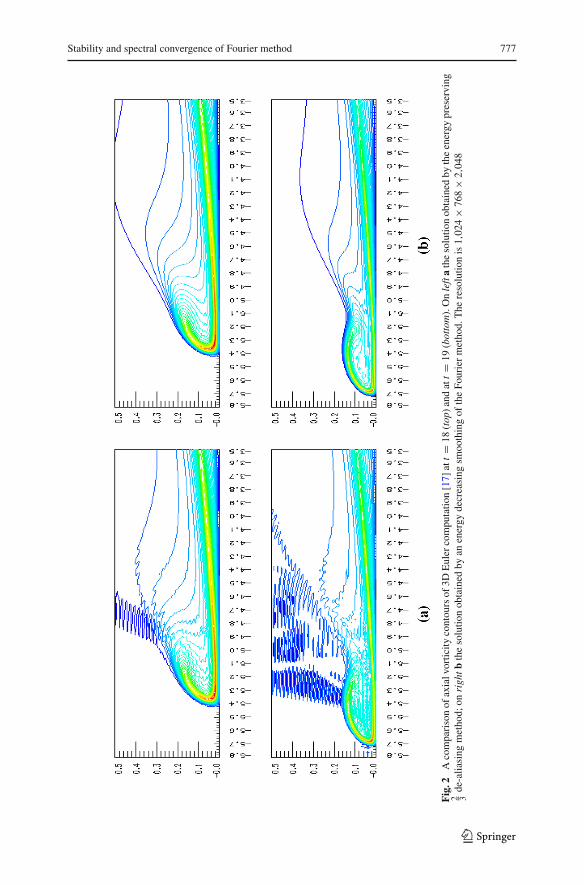
The similar scenario of quadratic entropy conservation in the context of Burgers’equations, is responsible for spurious oscillations, and its detailed analysis can befound in [23] after [29]. Here, enforcing energy conservation at the “critical” timewhen Euler solutions seem to lose sufficient smoothness leads to nonlinear instabilitywhich manifests itself through oscillations noticeable throughout the computationaldomain, in agreement with the numerical evidence observed in [17], see Fig. 2a below.The precise large-time behavior of the (pseudo-) spectral approximations is intimatelyrelated to a proper albeit yet unclear notion of propagating smoothness for solutionsof Euler equations which, even if they do not explicitly blow up, may exhibit spuriousoscillations due to the amplification factor in higher norms.

5 The spectral viscosity method: stability and spectral convergence

The nonlinear instability results in Sects. 3.2 and 4.2 emphasize the competitionbetween spectral convergence for smooth solutions vs. nonlinear instabilities for prob-lems which lack sufficient smoothness. One class of methods for nonlinear evolutionequations which entertain both—spectral convergence and nonlinear stability, is theclass spectral viscosity (SV) methods, introduced in [43]. We demonstrate the SVmethod in the context of Burgers equation,

∂

∂tuN (x, t)+ 1

2

∂

∂x

(ψN

[u2

N

](x, t)

)= SV [uN ](x, t), x ∈ T([0, 2π)). (5.1a)

On the right of (5.1a) we have added a judicious amount of spectral viscosity of order2r :

SV [uN ](x, t) := −N∑

|k|≤N

σ

( |k|N

)

uk(t)eikx , σ (ξ) �

(

|ξ |2r − 1

N

)

+, r ≥ 1

(5.1b)Without it, the pseudo-spectral solution will develops spurious Gibbs oscillationsafter the formation of shocks. Observe that the spectral viscosity term in (5.1b) adds aspectrally small amount of numerical dissipation for high modes, k � 1 (in contrast for”standard” finite-order amount of numerical dissipation in finite-difference methods),

‖SV [w]‖Hα � N 1−(α−β)(1− 12r )‖w‖Hβ , ∀β � α − 1 ∈ R.

123


Fig

.2A

com

pari

son

ofax

ialv

ortic

ityco

ntou

rsof

3DE

uler

com

puta

tion

[17]

att=

18(t

op)a

ndat

t=

19(b

otto

m).

On

left

ath

eso

lutio

nob

tain

edby

the

ener

gypr

eser

ving

2 3de

-alia

sing

met

hod;

onri

ghtb

the

solu

tion

obta

ined

byan

ener

gyde

crea

sing

smoo

thin

gof

the

Four

ier

met

hod.

The

reso

lutio

nis

1,02

4×

768

×2,

048

123


Indeed, the low-pass SV filter on the right of (5.1a) vanishes for modes |k| ≤N (2r−1)/2r , which in turn leads to spectral convergence for smooth solutions. Arguingalong the lines of Theorem 3.3 we state the following.

Theorem 5.1 (Spectral convergence for smooth solutions of Burgers’ equations)Consider the Burgers equation (3.1), with a smooth solution u(·, t) ∈ L∞([0, Tc],C1+α(0, 2π ]). Then its spectral viscosity approximation (5.1),

d

dtuN (xν, t)+ 1

2

∂

∂x

(ψN

[u2

N

](x, t)

)∣∣x=xν

= SV [uN ](xν, t), ν = 0, 1, . . . , 2N .

converges, ‖uN (·, t) − u(·, t)‖L2 → 0 for 0 ≤ t ≤ Tc and the following spectralconvergence rate estimate holds for all s > 3

2 ,

‖uN (·, t)− u(·, t)‖2

� e∫ t

0 |ux (·,τ )|∞dτ(

N−2s‖u(·, 0)‖2Hs + N

2r−12r ( 3

2 −s) maxτ≤t

‖u(·, τ )‖Hs

)

, s >3

2.

At the same time, spectral viscosity is strong enough to enforce a sufficient amountof L2 energy dissipation, which in turn implies convergence after the formation ofshock discontinuities. We quote below the convergence statement of the hyper-SVmethod.

Theorem 5.2 (Convergence of the hyper-SV method for Burgers equation [43,45,47])Let u be the unique entropy solution of the inviscid Burgers equation (3.1), subject touniformly bounded initial data u0, and let uN be the spectral viscosity approximation(5.1) subject to L∞ data uN (0) ≈ u0. Then, if uN remains uniformly bounded5 itconverges to the unique entropy solution, ‖uN (·, t)− u(·, t)‖L2 → 0.

Remark 5.3 We note that unlike the 2/3 de-aliasing method, the SV method doesnot completely remove the high-frequencies but instead, it introduces “just the rightamount” of smoothing for |k| � 1 which enables to balance spectral accuracy withnonlinear stability. The SV method can be viewed as a proper smoothing whichaddresses the instability of general smoothing of the pseudo-spectral Fourier methodsought in Remark 3.5. Moreover, even after the formation of shock discontinuities, theSV solution still contains highly accurate information of the exact entropy solutionwhich can be extracted by post-processing [41].

Similar results of spectral convergence of SV methods hold in the context of incom-pressible Euler equations [2,18,38],

∂

∂tuN + P∇xψN (SuN ⊗ SuN ) = SV [uN ],

SV [uN ](x, t) := −N∑

|k|≤N

σ

( |k|N

)

uk(t)eik·x. (5.2)

5 The question of uniform boundedness of uN was proved for the second order SV method, correspondingto r = 1, in [44], but it remains open for the hyper SV case with r > 1.

123


In contrast to the spurious oscillations with the 2/3 methods shown in Fig. 2a, theoscillations-free results in Fig. 2b correspond to the proper amount of smoothingemployed in [17]. Thus, the issue of adding “just the right amount” of hyper-viscosityis particularly relevant in this context of Large Eddy Simulation (LES) for highlyturbulent flows, when one needs to strike a balance between a sufficient amount ofnumerical dissipation for stability without giving up on high-order accuracy for phys-ically relevant Euler (and Navier–Stokes solutions). The SV method in (5.2) adds thisbalanced amount of hyper-viscosity [16,18,34,38,40].

6 Beyond quadratic nonlinearities: 1D isentropic equations

We consider the one-dimensional isentropic equations in Lagrangian coordinate,

∂

∂tu + ∂

∂xq(v) = 0, q ′(v) > 0 (6.1a)

∂

∂tv + ∂

∂xu = 0, (6.1b)

which is approximated by the spectral method

∂

∂tuN + ∂

∂xq(vN ) = (I − PN )q(vN ), (6.2a)

∂

∂tvN + ∂

∂xuN = 0. (6.2b)

Denote by U the vector of conservative variables, U := (u, v) , by F(U ) thecorresponding flux, F(U ) := (q(v), u) and let η(U ) be the entropy η(U ) := 1

2 |u|2+Q(v), Q′(v) = q(v). Multiplying the system by ∇Uη(U ) and integrating gives:

d

dt

∫ ( |uN |22

+ uN ∂x q(vN )+ q(vN )∂x uN

)

dx =∫

(I − PN )q(vN )uN dx = 0

and hence there the total entropy is conserved for both the exact an approximatesolutions6

∂t

∫

η(U )dx = 0 and ∂t

∫

η(UN )dx = 0.

Continuing as in DiPerna–Chen [6,9,12], we write

∂t

∫(η(UN )− η(U )− ⟨η′(U ),Un − U

⟩)dx

=∫⟨η′′(U )Ut , (UN − U )

⟩dx −

∫⟨η′(U ), (UN )t − Ut

⟩dx

6 This intriguing property seems specific to the isentropic equation in Lagrangian coordinate.

123


= −∫⟨η′′(U )F(U )x ,UN − U

⟩dx

−∫⟨η′(U ), F(UN ))x − F(U )x

⟩dx + error term

=: I1 + I2 + I3 (6.3)

The first two terms on the right amount to

|I1 + I2| =∣∣∣∣

∫⟨η′′(U )F(U )x ,UN − U

⟩dx +

∫⟨η′(U ), F(UN )x − F(U )x

⟩dx

∣∣∣∣

=∣∣∣∣

∫⟨η′′(U )F ′(U )Ux ,UN − U

⟩dx − ⟨η′′(U )Ux , F(UN )− F(U )

⟩dx

∣∣∣∣

=∣∣∣∣

∫⟨η′′(U )F ′(U )Ux ,UN −U

⟩dx−

⟨η′′(U )Ux , F ′(U )Ux +O‖UN −U‖2

⟩dx

∣∣∣∣ .

Since the entropy Hessian symmetrize the system, one has η′′(U )F ′(U ) =F ′(U )η′′(U ), and we conclude that the last expression does not exceed

|I1 + I2| =∣∣∣∣

∫⟨η′′(U )F ′(U )Ux ,UN − U

⟩dx − ⟨η′′(U )Ux , F(UN )− F(U )

⟩dx

∣∣∣∣

� ‖U‖C1‖UN − U‖2

On the other hand

I3 = error term =∫

(I − PN )qx (vN )(u − uN )dx =∫

∂x q(vN )(I − PN )ux dx

which goes to zero for sufficiently smooth u ∈ C1+α . Inserting the last two boundinto (6.3) we find that

∂t

∫(η(UN )− η(U )− ⟨η′(U ),Un − U

⟩)dx � ‖U‖C1‖UN − U‖2 + o(1).

By strict convexity, the integrand on the left is of order ∼ ‖UN −U‖2 and we concludethe following.

Theorem 6.1 Assume that for 0 < t < Tc, the solution of the isentropic Euler equa-tions (6.1) is smooth, U (·, t) ∈ L∞([0, Tc),C1+α(0, 2π ]). Then, its spectral approx-imation (6.2) converge in L∞

t L2x ,

‖UN (·, t)− U (·, t)‖L2 → 0, 0 ≤ t < Tc.

Acknowledgments E. T. Research was supported in part by NSF grants DMS10-08397, RNMS11-07444(KI-Net) and ONR grant #N00014-1210318.

123


References

1. Abarbanel, S., Gottlieb, D., Tadmor, E.: Spectral methods for discontinuous problems “Numericalmethods for fluid dynamics II”. In: Morton, K.W., Baines, M.J. (eds.) Proceedings of the 1985 Con-ference on Numerical methods for fluid dynamics. Clarendon Press, Oxford, pp. 129–153 (1986)

2. Avrin, J., Xiao, C.: Convergence of Galerkin solutions and continuous dependence on data in spectrallyhyperviscous models of 3D turbulent flow. J. Differ. Equ. 247, 2778–2798 (2009)

3. Bardos, C., Titi, E.: Loss of smoothness and energy conserving rough weak solutions for the 3D Eulerequations. DCDS Ser. 5 3(2), 185–197 (2010)

4. Buckmaster, T.: Onsager’s conjecture almost everywhere in time. arXiv:1304.1049 (2013)5. De Lellis, C., Székelyhidi Jr, L.: On admissibility criteria for weak solutions of the Euler equations.

Arch. Ration. Mech. Anal. 195(1), 225–260 (2010)6. Chen, G.-Q.: Remarks on DiPerna’s paper “Convergence of the viscosity method for isentropic gas

dynamics”. Proc. AMS 125(10), 2981–2986 (1997)7. Constantin, P.: On the Euler equations of incompressible fluids. Bull. AMS 44(4), 603–621 (2007)8. Constantin, P., Weinan, E., Titi, E.S.: Onsager’s conjecture on the energy conservation for solutions of

Euler’s equation. Commun. Math. Phys. 165, 207–209 (1994)9. Dafermos, C.: The second law of thermodynamics and stability. Arch. Ration. Mech. Anal. 70(199),

167–17910. De Lellis, C., Székelyhidi, L.: The h-principle and the equations of fluid dynamics. Bull. Am. Math.

Soc. 49, 347–375 (2012)11. DeVore, R., Lorentz, G.G.: Constructive Approximation, Springer Grundlehren, vol. 303 (1993)12. DiPerna, R.: Convergence of the viscosity method for isentropic gas dynamics. Commun. Math. Phys.

91, 1–30 (1983)13. Eyink, G.L.: Energy dissipation without viscosity in ideal hydrodynamics, I. Fourier analysis and local

energy transfer. Phys. D 78, 222–240 (1994)14. Goodman, J., Hou, T., Tadmor, E.: On the stability of the unsmoothed Fourier method for hyperbolic

equations. Numer. Math. 67(1), 93–129 (1994)15. Gottlieb, D., Orzag, S.: Numerical Analysis of Spectral Methods : Theory and Applications. SIAM,

Philadelphia (1977)16. Guermond, J.-L., Prudhomme, S.: Mathematical analysis of a spectral hyperviscosity LES model for

the simulation of turbulent flows. Math. Model. Numer. Anal. 37, 893–908 (2003)17. Hou, T.Y., Li, R.: Computing nearly singular solutions using pseudo-spectral methods. J. Comput.

Phys. 226, 379–397 (2007)18. Karamanos, G.-S., Karniadakis, G.E.: A spectral vanishing viscosity method for large eddy-

simulations. J. Comput. Phys. 163, 22–50 (2000)19. Kerr, R.M.: Evidence for a singularity of the three dimensional, incompressible Euler equations. Phys.

Fluids 5(7), 1725–1746 (1993)20. Kerr, R.M.: Velocity and scaling of collapsing Euler vortices. Phys. Fluids 17, 075103–114 (2005)21. Kerr, R.M., Hussain, F.: Simulation of vortex reconnection. Phys. D 37, 474 (1989)22. Kreiss, H.-O., Oliger, J.: Comparison of accurate methods for the integration of hyperbolic equations.

Tellus 24, 199–215 (1972)23. Lax, P.D.: On dispersive difference schemes. Phys. D 18, 250–254 (1986)24. Lions, P.L.: Mathematical Topics in Fluid Mechanics, vol. 1. Incompressible Models, Oxford Lecture

Series in Mathematics and its Applications, Oxford (1996)25. Lopes Filho, M., Nussenzveig, H.J., Tadmor, E.: Approximate solutions of the incompressible Euler

equations with no concentrations. Annales De L’institut Henri Poincare (c) Non Linear Analysis 17,371–412 (2000)

26. Majda, A., McDonough, J.M., Osher, S.: The Fourier method for non-smooth initial data. Math.Comput. 32, 1041 (1978)

27. Mock, M., Lax, P.D.: The computation of discontinuous solutions of linear hyperbolic equations.Commun. Pure Appl. Math. 31, 423–430 (1978)

28. Murat, F.: Compacit’e par compensation. Ann. Sc. Norm. Super. Pisa, Cl. Sci., IV. Ser. 5, 489–507(1978)

29. von Neumann, J.: Proposed and analysis of a new numerical method in the treatment of hydrodynamicalshock problem, vol. VI, Collected Works, pp. 361–379. Pergamon, London (1963)

123

http://arxiv.org/abs/1304.1049


30. Ohlsson, J., Schlatter, P., Fischer, P.F., Henningson, D.S.: Stabilization of the spectral-element methodin turbulent flow simulation, ICOSAHOM (2010)

31. Onsager, L.: Statistical hydrodynamics, Nuovo Cimento (9), 6 Supplemento, 2(Convegno Inter-nazionale di Meccanica Statistica), pp. 279–287 (1949)

32. Orszag, S.: Comparison of pseudospectral and spectral approximations. Stud. Appl. Math. 51, 253–259(1972)

33. Panov, E.: Uniqueness of the solution of the Cauchy problem for a first-order quasilinear equation withan admissible strictly convex entropy. Mat. Zametki 55(5), 116–129 (1994) [translation in Math. Notes55(5–6), 517–525 (1994)]

34. Pasquetti, R., Severac, E., Serre, E., Bontoux, P., Schafer, M.: From stratified wakes to rotor-statorflows by an SVV-LES method. Theor. Commput. Fluid Dyn. 22(3–4), 261–273 (2007)

35. Pereira, R.M., Nguyen van yen, R., Farge, M., Schneider, K.: Wavelet methods to eliminate resonancesin the Galerkin-truncated Burgers and Euler equations. Phys. Rev. E 87, 033017 (2013)

36. Ray, S.S., Frisch, U., Nazarenko, S., Matsumuto, T.: Resonance phenomenon for the Galerkin-truncatedBurgers and Euler equations. Phys. Rev. E 84, 016301 (2011)

37. Scheffer, V.: An inviscid flow with compact support in space-time. J. Geom. Anal. 3, 343–401 (1993)38. Severac, E., Serre, E.: A spectral vanishing viscosity for the LES of turbulent flows within rotating

cavities. J. Comput. Phys. 226, 1234–1255 (2007)39. Shnirelman, A.: On the nonuniqueness of weak solutions of the Euler equations. Commun. Pure Appl.

Math. 50, 1261–1286 (1997)40. Sirisup, S., Karniadakis, G.E.: A spectral viscosity method for correcting the long-term behavior of

POD models. J. Comput. Phys. 194, 92–116 (2004)41. Shu, C.-W., Wong, P.S.: A note on the accuracy of spectral method applied to nonlinear conservation

laws. J. Sci. Comput. 10(3), 357–369 (1995)42. Tadmor, E.: Stability analysis of finite-difference, pseudospectral and Fourier–Galerkin approximations

for time-dependent problems. SIAM Rev. 29, 525–555 (1987)43. Tadmor, E.: Convergence of spectral methods for nonlinear conservation laws. SINUM 26, 30–44

(1989)44. Tadmor, E.: Total variation and error estimates for spectral viscosity approximations. Math. Comput.

60, 245–256 (1993)45. Tadmor, E.: Super viscosity and spectral approximations of nonlinear conservation laws. In: Baines, J.,

Morton, K.W. (eds.) Numerical Methods for Fluid Dynamics IV, Proceedings of the 1992 Conferenceon Numerical Methods for Fluid Dynamics, pp. 69–82. Clarendon Press, Oxford (1993)

46. Tadmor, E.: Spectral methods for hyperbolic problems, Methods numeriques d’ordre eleve pour lesondes en regime transitoire, Lecture notes delivered at Ecole des Ondes, INRIA—Rocquencourt (1994)

47. Tadmor, E.: Burgers’ equation with vanishing hyper-viscosity. Commun. Math. Sci. 2(2), 317–324(2004)

48. Tadmor, E.: Filters, mollifiers and the computation of the Gibbs phenomenon. Acta Numer. 16, 305–378(2007)

49. Tartar, L.: Compensated compactness and applications to partial differential equations. In: Knopps, R.J.(ed.) Research Notes in Mathematics 39, Nonlinear Analysis and Mechanics, Heriott-Watt Symposium,vol. 4. Pittman Press, pp. 136–211 (1979)

50. Tartar, L.: The compensated compactness method for a scalar hyperbolic equation, Carnegie MellonUniv. Lecture notes, pp. 87–20 (1987)

123

Stability and spectral convergence of Fourier method for …€¦ · Stability and spectral...

Documents

Transcript of Stability and spectral convergence of Fourier method for …€¦ · Stability and spectral...