1

1

Fourier Series. Spectral Analysis of Periodic Signals

The response of continuous-time linear invariant systems to the complex exponential with unitary

magnitude

2

• response of a continuous-time LTI system at a certain signal:– differential equation – convolution product of the input signal with impulse

response. • input signal periodic: decompose into a series

of simpler components, – response of the system at each component– synthesis of partial responses.

• frequency domain: Fourier series

2

3

h(t)( ) 0

0

,

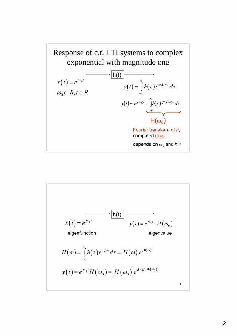
j tx t eR t R

ω

ω=

∈ ∈( ) ( ) ( )0j ty t h e dω ττ τ

∞−

−∞

= ∫

( ) ( )∫∞

∞−

−⋅= ττ τωω dehety jtj 00

H(ω0)Fourier transform of h, computed in ω0

depends on ω0 and h

Response of c.t. LTI systems to complex exponential with magnitude one

4

h(t)( ) 0j tx t e ω= ( ) ( )0

0j ty t e Hω ω= ⋅

eigenfunction eigenvalue

( ) ( ) ( ) ( )jjH h e d H e ωωτω τ τ ω∞

Φ−

−∞

= =∫

( ) ( ) ( ) ( )( )0 000 0

j tj ty t e H H e ω ωω ω ω +Φ= =

3

5

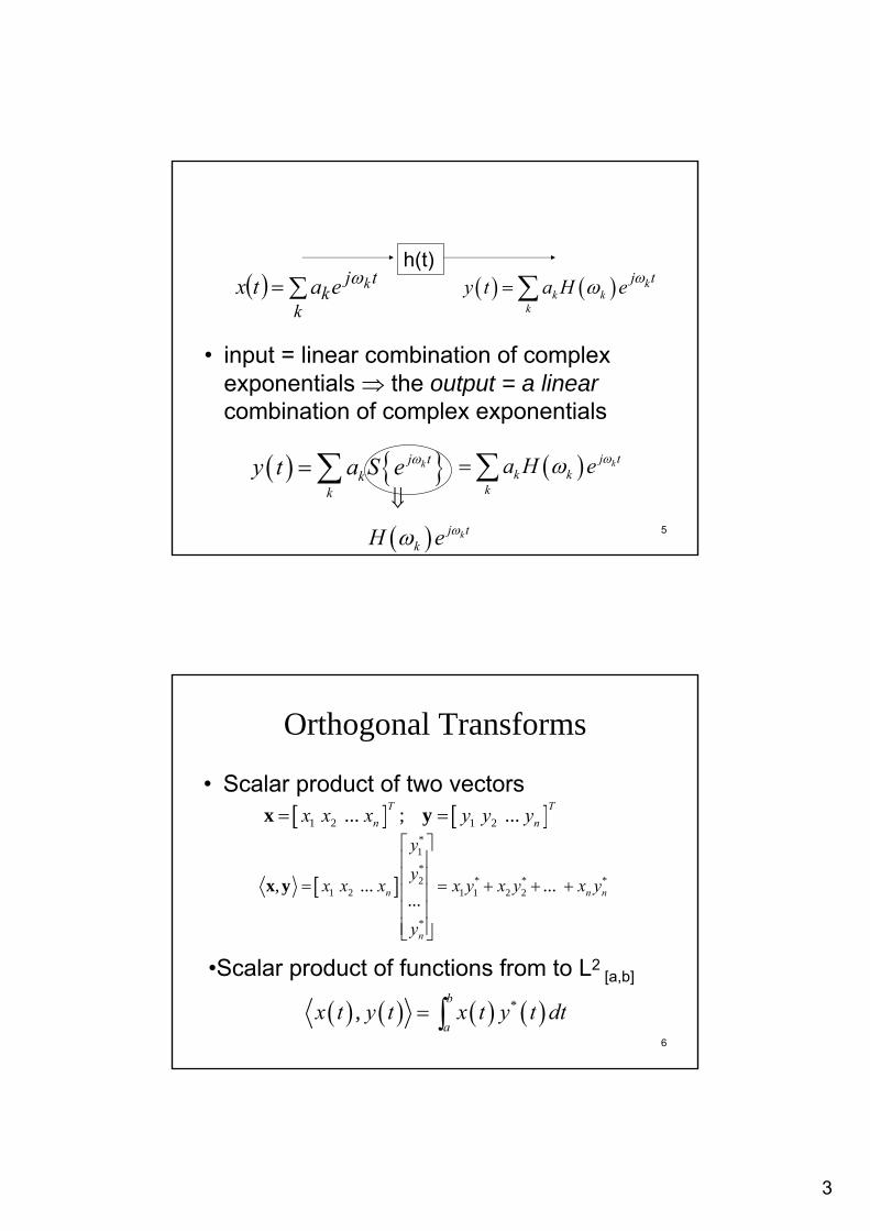
• input = linear combination of complex exponentials ⇒ the output = a linearcombination of complex exponentials

( ) { }kj tk

ky t a S e ω=∑

( )

kj tkH e

⇓ωω

( ) kj tk k

ka H e ωω=∑

h(t)( ) ∑=

k

tjk keatx ω ( ) ( )k k

k

kj ty t a H e ωω=∑

6

Orthogonal Transforms

• Scalar product of two vectors[ ] [ ]1 2 1 2 ... ; ... T T

n nx x x y y y= =x y

[ ]

*1*

* * *21 2 1 1 2 2

*

, ... ... ...n n n

n

y

yx x x x y x y x y

y

⎡ ⎤⎢ ⎥⎢ ⎥= = + + +⎢ ⎥⎢ ⎥⎢ ⎥⎣ ⎦

x y

•Scalar product of functions from to L2[a,b]

( ) ( ) ( ) ( )*,b

ax t y t x t y t dt= ∫

4

7

• Properties*

*

*

1 1 1 1

i) , , ,

ii) , , , ,

iii) , , ,

iv) , , ,

v) , , .n m n m

k k l l k l k lk l k l

x y y x

x y z x y x z

x y x y

x y x y C

x y x y

λ λ

λ λ λ

α β α β= = = =

=

+ = +

=

= ∀ ∈

=∑ ∑ ∑∑

8

Proof

∑ ∑

∑ ∑∑ ∑

∑ ∑∑ ∑

∑ ∑∑ ∑

= =

= == =

= == =

= == =

=

===

===

==

n

k

m

llklk

i

m

l

n

kklkl

iiim

l

n

kkkll

ii

m

l

n

kkkll

m

l

il

n

kkkl

iii

m

lll

n

kkk

iin

k

m

lllkk

yx

xyxy

xyyx

yxyx

1 1

*)

1 1

**)

1 1

**)

1

*

1

*

1

)

1

*)

1 1

)

1 1

,

,,

,,

,,

βα

αβαβ

αβαβ

βαβα

5

9

• The norm

• Rules i)-iv) apply for the space L2, so the norms ||x|| are finite.

( )

2 2 2 2 21 1 1

1

22

, ...n

kk

b

a

x x x x

x x t dt

=

= = + + + =

=

∑

∫

x x x

10

Hilbert space

• A structure frequently used in approximation theory.

• Space composed by vectors. Each of them has its norm.

• This norm is defined with the aid of the scalar product of vectors denoted by <>.

6

11

1) Finite dimensional Hilbert space, withdimension n

( ) ( )

( )

1 2 1 2

*1*2

* *1 2

1

*

22

1

, ,..., , , ,..., ,

., , ,..., ,

.

.

,

T Tn n

nT

n k kk

n

n

kk

x x x x y y y y

yy

x y x y x x x x y

y

x x x x

=

=

= =

⎡ ⎤⎢ ⎥⎢ ⎥⎢ ⎥

= = =⎢ ⎥⎢ ⎥⎢ ⎥⎢ ⎥⎢ ⎥⎣ ⎦

= =

∑

∑

12

• The scalar product <x,y>-matrices product of the transposed of the x with the conjugate of the y.

• The squared norm of x = the scalar product <x,x>.

• Model for: – Discrete time signals on the interval [0, n-1]– or periodic (with period n) discrete time

signals.

7

13

2) Finite dimensional Hilbert space of finite energy signal with finite duration

( )⎭⎬⎫

⎩⎨⎧ ∞<→ ∫

ba dttxCRx 2:

[ ]

( ) ( ) ( ) ( ) ( ) ( )

2,

2 2*

, ;

, ; .

a b

b b

a a

x y L

x t y t x t y t dt x t x t dt

∈

= =∫ ∫

•Model for: –continuous time signals on the interval [ a,b] or –periodic (with period T=b-a) continuous time signals

14

Orthogonal vectors

1 2 1 2 ; , cos

x x y yα

= + = +

=

x i j y i jx y x y

,cosα =

⋅x y

x y

• For two bidimensional vectors

α-angle between vectors

8

15

• If the two vectors are perpendicular (orthogonal) then <x, y> = 0

• If the scalar product is 0 => the two vectors are orthogonal.

• Orthogonality condition:

, 0= ⇔ ⊥x y x y

16

Orthogonal functions

• Consider two signals defined on (0,T0), with T0=2π/ω0 -- space L2

[0,T0]

• The scalar product is 0

( ) ( )0 0cos ; sinx t t y t tω ω= =

( ) ( ) ( )

( )

0 0

0

0 0 0 0 00 0

0

0 00

1cos ,sin cos sin sin 22

cos 2 1 cos 4 04 4

T T

T

t t t t dt t dt

t

ω ω ω ω ω

ω πω ω

= =

−= − = =

∫ ∫

9

17

Complete space

• A system U={uk} of orthogonal vectors two by two from a Hilbert space H is completein H if:

• there is no other vector x∈H-U , orthogonal on all the vectors from U only the vector 0

, 0 0, if .ku x x x H U= ⇔ = ∈ −

18

Orthogonal basis of Hilbert space

• Each complete system U is an orthogonal basis of H.

• Any element x from H can be expressed like a linear combination of elements of U uniquely

, .k kk

x H x a u∀ ∈ =∑

10

19

Examples of basis

• The unity vectors {i, j, k} are a basis in the three-dimensional space.

• The set of complex exponential{e jkω0t}|k∈Z with frequency kω0 is an infinite dimensional basis for the periodic continuous time signals of period T0

20

Pythagoras’ theorem in the Hilbert space. Relation between distance and scalar

product• Consider two vectors in the Hilbert space• Their difference is

= −d x y

( ) 22 ,d = −x y x y

11

21

• For vectors/functions in the Hilbert space

• Pythagoras’ theorem in the Hilbert space. If x and y are orthogonal

( ) { }2 2 22 , 2Re ,d x y x y x x y y= − = − +

( ) 2 22 ,d x y x y= +

22

Examples for Pythagoras’ theoremin the Hilbert space L2

[0,T0]

• orthogonal signalshave the same norm

• Pythagoras’ theorem

( ) ( )0 0cos and sint tω ω

( ) ( ) ( )

( )

0 0

0 0

2 020

0 0

00 0 0

0

1 cos 2cos

21 1 sin 2

2 2 2 2

T T

T T

tx t t dt dt

Tt t

ωω

ωω

+= = =

= + ⋅ =

∫ ∫

( )2 0 00 0 0cos ,sin .

2 2T Td t t Tω ω = + =

12

23

• non-orthogonal signals do not satisfy Pythagoras’ theorem.

• signals on L2[0,T0]

are not orthogonal:( ) ( )0 0cos and cost tω ω−

02 0

0 0 00

cos , cos cos .2

T Tt t tdtω ω ω− = − = −∫

( ) { }2 22 , 2Re ,d x y x x y y= − +Should be zero, but it’s not

24

Examples for Pithagoras’ theorem

• square distance

||x||2= ||y||2 = T0/2• scalar product <x,y>= –T0/2 . • ⇒ the square distance

( ) { } 222 ,Re2, yyxxyxd +−=

( )2 0 0 00 0 0cos , cos 2 2 .

2 2 2T T Td t t Tω ω ⎛ ⎞− = + − − =⎜ ⎟

⎝ ⎠

13

25( ) ( )0 0 0 0cos ,sin cos , cos .d t t d t tω ω ω ω< −

26

Schwarz’s inequality in the Hilbert space

• with equality holding if and only if x and yare linearly dependent, i.e.

y=kx, • for some scalar k

,x y x y≤ ⋅

(Cauchy- Bunyakovsky-Schwarz inequality)

14

27

Examples for Schwarz’s inequality1. Orthogonal signals L2

[0,T0]

• product of the norms

( ) ( )0cosx t tω= ( ) ( )0siny t tω=

( ) ( ), 0x t y t =

( ) ( ) 0 0 0

2 2 2T T Tx t y t⋅ = ⋅ =

28

• Schwarz’s inequality is verified

0<T0/2

• There is no k such that y(t) = k⋅x(t)• So, in this case the Schwarz’s inequality

can not become equality

15

29

Examples for Schwarz’s inequality2. Non-orthogonal signals L2

[0,T0]

• there exists a value k=-1 - Schwarz’s inequality becomes an equality.

( ) ( ) ( ) ( )0 0cos and cosx t t y t tω ω= = −

( ) ( )y t x t⇒ = −

( ) ( )0 0; 2 2T Tx t y t= =

( ) ( ) 0 0,2 2T Tx t y t = − =

30

Optimal approximation in Hilbert space

• n-dimensional Hilbert space, with orthogonal basis

• U is orthonormal

{ }1 2, ,..., nU u u u=

2 , ,0,l

k lu k lu u

k l

⎧ =⎪= ⎨≠⎪⎩

2 1 and , .k k ku c x u= =

16

31

• Vector=unique linear combination of vectors from U

• The coefficients ck

1

n

k kk

x c u=

= ∑

{ }2

,, 1, 2, ..., , .k

kk

x uc k n x H

u= ∈ ∀ ∈

32

Optimal approximation in Hilbert space

• Approximation: represent n-dimensional vector x using only m elements, m<n

• Best approximation: truncation of its series decomposition

• increase m (number of terms in the approximation) ⇒ the error decreases & the approximation becomes better

∑=

λ=m

kkkux~

1

, 1,..., .k kc k mλ = =

17

33

• approximation error

• norm

• minimize the norm of the error

e x x= −

( ) 2 22 ,d x x x x e= − =

( ),e d x x=

Proof

34

( ) 22

1 1

2 * *

1 1 1 1

, , ,

, , ,

m m

k k i ik i

m m m m

k k i i k i k ik i k i

d x x e e e x u x u

x u x x u u u

λ λ

λ λ λ λ

= =

= = = =

= = = − −

= − − +

∑ ∑

∑ ∑ ∑∑

( )2 * 2 2*

1 1

, ,m m

k k k k k kk k

x x u x u uλ λ λ= =

= − + +∑ ∑

18

35

• Select coefficients λk to minimize d2. • Partial derivates of d2 (function of λk ) = 0

{ }

( )

2

22 2 2 22

min 21 1

,, 1 2 , ,

,, .

kk k

k

m mk

k kk kk

x uλ c k , , ..., m m n

u

x ud x x x x c u

u= =

= = ∈ <

= − = −∑ ∑

36

Projection theorem

• the approximation error is orthogonal onso it’s orthogonal on the approximation m-dimensional subspace

( ) 2 22min

2 2 2

2 2 2

,d x x x x

x x x x

x x x x

= −

− = −

⇒ = + −

x~

19

37

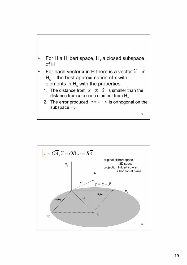
• For H a Hilbert space, Hs a closed subspaceof H

• For each vector x in H there is a vector in Hs = the best approximation of x withelements in Hs with the properties

1. The distance from is smaller than the distance from x to each element from Hs

2. The error produced is orthogonal on thesubspace Hs

x~

to x x

e x x= −

38

e x x= −x

x1 1a u2 2a u 2u

1u

3u

A

B

ABe,BOx~,AOx ===original Hilbert space

= 3D space projection Hilbert space

= horizontal plane

20

39

2

1 1 1 1

22

1

, , ,n n n n

k k l l k l k lk l k l

n

k kk

x x x c u c u c c u u

c u

= = = =

=

= = =

=

∑ ∑ ∑∑

∑

( ) 2 2 22min min

2 2 2 2 2 2

1 1 1

,n m n

k k k k k kk k k m

d x x e x x

c u c u c u= = = +

= = − =

= − =∑ ∑ ∑

40

Infinite dimensional Hilbert spaces

• orthogonal basis in a finite dimensional space, subspace of Hilbert space

• The decomposition of signal x:

( ){ }, , N kU u t k N N= = −

( ) ( ) ( ) ( )( ) 2

,, with k

k k kk k

x t u tx t c u t c

u t

∞

=−∞

= =∑

21

41

The case of infinite dimensional spaces

• Approximation signal in a finite dimensional Hilbert space of dimension 2N+1:

• Like before, we have

• for minimum error

( ) ( )N

N k kk N

x t u tλ=−

= ∑

{ }, , 1,...,0,1,...,k kc k N N Nλ = ∈ − − +

( ) ( ) ( ) ( )2 2 22N

N k kk N

x t x t x t c u t=−

− = − ∑

42

• But:

• The error becomes:

( ) ( ) ( ) ( ) ( )

( )

2

22

, ,k k l lk l

k kk

x t x t x t c u t c u t

c u t

∞ ∞

=−∞ =−∞

∞

=−∞

= =

=

∑ ∑

∑

( ) ( ) ( ) ( )

( )

2 2 22 2

22

N

N k k k kk k N

k kk N

x t x t c u t c u t

c u t

∞

=−∞ =−

∀ >

− = −

=

∑ ∑

∑

Parseval’s relation

22

43

The case of infinite dimensional spaces

• More terms (N high) ⇒ error decreases• We have :

• Bessel’s inequality.

( ) ( )2 22 2N

N k kk N

x t c u x t=−

= ≤∑

44

• The approximation signal convergesin mean square to x(t)

( ) ( ) [ ]

( ) ( )

2 2,

2 2

2

< because

lim 0

lim 0

a b

k kN k N

NN

x t x t L

c u

x t x t

→∞∀ >

→∞

∞ ∈

⇒ =

⇒ − =

∑

( )Nx t

( ) ( )l.i .m. NNx t x t

→∞=

23

45

Remarks

1. We havePitagora’s theorem: orthogonality between the best

approximation and the approximation error

2. Parseval’s relation ( Rayleigh’s energytheorem)

3. The best approximation is obtained bytruncating the series decomposition

( ) ( ) ( ) ( )2 2 2N Nx t x t x t x t= + −

( ) ( ) ( ), 0N Nx t x t x t− =

( ) ( )2 22k k

kW x t c u t

∞

=−∞

= = ∑

46

Fourier Series

• consider in the space an orthogonal basis :

• The elements are orthogonal and the set is complete.

[ ]0

20,TL

( ) 0 , jk tku t e k Zω= ∈

( )

( )

0

00 0

00

20

0,,

,

The norm

Tj k l tjk t jl t

k

k le e e

T k l

u t T

ωω ω − ≠⎧= = ⎨ =⎩

=

∫

24

47

Exponential Fourier series

• For a periodic signal x(t)=x(t+T0)

( ) ( )0 0

0

00

1 2, jk t jk tk k

k T

x t c e c x t e dtT T

ω ω ω∞

−

=−∞ 0

π= ↔ = =∑ ∫

( ) ( )

( )( )

0

0

0

00

20

, 1

jk tk k k

k k

jk tjk t

k jk tT

x t c u t c e

x t ec x t e dt

Te

ω

ωω

ω

∞ ∞

=−∞ =−∞

−

= =

= =

∑ ∑

∫

48

Trigonometric Fourier series

• Euler’s relations

• An orthogonal basis of the same space is:

• the elements are orthogonal and the set is complete.

( ) ( ){ } Nktktk, U ∈= 00 sin ,cos1 ωω

( ) ( ) ( ) ( )0 0 0 00 0

1 1cos ; sin2 2

jk t jk t jk t jk tk t e e k t e ej

ω ω ω ωω ω− −= + = −

25

49

Trigonometric Fourier series

• The norms of the basis’ elements are:

( ) ( )

( ) ( )

0

0

0

0

0

0

22 2

02

22 2 0

0 02

22 2 0

0 02

1 1 ;

cos cos ; 2

sin sin ;2

T

T

T

T

T

T

dt T

Tk t k t dt

Tk t k t dt

ω ω

ω ω

−

−

−

= =

= =

= =

∫

∫

∫

50

Trigonometric Fourier series

• So, any periodic signal of period T0 can be expressed in the form:

( ) ( ) ( )( )∑∞

=++⋅=

1000 sincos1

kkk tkbtkaatx ωω

26

51

Trigonometric Fourier series

• the coefficients are :

( ) ( )

( ) ( )( )

( ) ( )

( ) ( )( )

( ) ( )

0

0

0

0 20

002

00

002

00

,1 1 , continuous component. 1

,cos 2 cos , cos

,sin 2 sin .sin

T

kT

kT

x ta x t dt

T

x t k ta x t k t dt

Tk t

x t k tb x t k t dt

Tk t

ωω

ω

ωω

ω

= =

= =

= =

∫

∫

∫

52

Remarks1. a0 - DC component of the signal x(t) 2. The signal with no DC component(a0 =0) has

only “oscillatory” components:

3. For real signals

( ) ( )0 01

cos sin ;k kk

x t a k t b k tω ω∞

=

= +∑

( ) ( )odd 0; even 0;k kx t a x t b− ⇒ = − ⇒ =

( ) ( )0 0

0 0

*

*

0 0

1 1jk t jk tk k

T T

c x t e dt x t e dt cT T

ω ω−−

⎡ ⎤= = =⎢ ⎥

⎢ ⎥⎣ ⎦∫ ∫

( ) ( )* *k kx t x t c c−= ⇒ =

27

53

4. the power of the signal x(t) - Parseval’srelation :

• another form of the Parseval’s relation:

( )0

2 22 2

010

12 2k k

Tk

a bP x t dt aT

∞

=

⎛ ⎞= = + +⎜ ⎟

⎝ ⎠∑∫

( )0

2 2 20

1 10 0 0

1k k

k k T

TWP c P c x tT T T

∞ ∞

= =

= = ⇒ = =∑ ∑ ∫

54

Harmonic Fourier Series

• Using the relation:

• the Fourier trigonometric series becomes:

• harmonic form.

( )2 20 0 0cos sin cosk k k k ka k t b k t a b k tω ω ω ϕ+ = + +

2 2tg . kk k k k

k

b A a ba

ϕ = − = +

( ) ( )∑∞

=+=

00cos

kkk tkAtx ϕω

28

55

Relations between coefficients

• For real signals we have

2 2

0 0 0

1 , 1 2

, 1;arg , 1 ; arg , 1;

; arg 0.

k k k k

k k

k k

k k

c a b A k

c c kc k c k

c a c

ϕϕ

−

−

= + = ≥

= ≤ −

= ≥= − ≤ −

= =

56

Spectrum diagrams

• represent periodic signals in the frequency domain.

( )0

00

2, 02

0,2

Ttx t

T t T

⎧ ≤ <⎪⎪= ⎨⎪ ≤ <⎪⎩

29

57

• DC component:

• The oscillatory component is odd

( )0

10

0

1, 02

1,2

Ttx t

T t T

⎧ ≤ <⎪⎪= ⎨⎪− ≤ <⎪⎩

00 =⇒≠ kak

( )0

0

2

0 0 00 0 0

1 1 2 1; T

T

a x t dt dt A aT T

= = = =∫ ∫

58

• the other coefficients

• or

2 0kb =

( ) ( )0

0

2

00

0 0 0 0 00

1 1cos2 4 4sin ; 1T k

kT

k tb x t k tdt kT T k T k

− −− ω= ω = ⋅ = ⋅ ≥

ω ω∫

( )2 14 ; 1, 2,3,...

2 1kb kk− = =− π

30

59

( ) ( ) ( ) 01

41 sin 2 12 1k

x t k tk

ωπ

∞

=

= + −⎡ ⎤⎣ ⎦−∑

( ) ( ) ( ) 01

41 cos 2 12 1 2k

x t k tk

πωπ

∞

=

⎡ ⎤= + − −⎢ ⎥− ⎣ ⎦∑

( ) ( )2 1

0

, 2 1 th order harmonics of frequency 2 1

kAk k ω

−

− −

60

Amplitude spectrum (kω0, Ak)

DC component

Fundamental

frequency 2π/T0

2nd

harmonic

3rd

harmonic

Harmonic Fourier series

31

61

Phase spectrum (kω0, ϕk)

Harmonic Fourier series

62

Amplitude spectrum (kω0, |ck|)

• obtained also with the complexexponential form of the Fourier series.

• The coefficients ck : ( )

( ) ( )

( )

0

0

0 0

0

0 00

2

0 0 0

2 22 1 2 1

2

1 1

1 11 1 2 ; 0

2 2; 1; ; 12 1 2 1

0, 0

T

kTjk t jk t

kT

j j

k k

k

c x t dt aT

c x t e dt e dt kT T jk

c e k c e kk k

c k

− ω − ω

π π−

− −

= = =

− −= = = ≠

π

= ≤ − = ≥− π − π

= ≠

∫

∫ ∫

32

63

Magnitude spectrum (kω0, |ck |)

negative frequencies

EVEN FUNCTION

2 12

2 1kck− =− π

64

Phase spectrum (kω0, ϕk )

• Another representation in the frequency domain. For the square wave we have:

ODD FUNCTION

( ) sgn2k kπ

ϕ = −

33

65

Other forms of Parseval’s relation

• complex exponential Fourier series :

• trigonometric & harmonic

( )0

2 2 2 20

00

1 2k kk kT

P x t dt c c cT

∞ ∞

=−∞ =

= = = +∑ ∑∫

( )0

2 2 222 2

0 01 10

12 2 2k k k

Tk k

a b AP a x t dt AT

∞ ∞

= =

⎛ ⎞= + + = = +⎜ ⎟

⎝ ⎠∑ ∑∫

66

• The power of this square wave

( )0

0

/ 22

0 0

1 1 4 24

T

T

P x t dt dtT

= = =∫ ∫

34

67

Power spectrum

• the association of the frequencies of its components with their powers– harmonic form (kω0, Ak

2/2)– complex exponential form (kω0, |ck|2)

68

Power spectrum with the harmonic Fourier series

squarewave

35

69

Power spectrum with the exponential Fourier series

70

• non-band-limited signal: – the signal has infinite frequency bandwidth. – The power decreases as the frequency

increases; it approaches zero only at infinite frequency

• effective bandwidth of the signal = positive frequency range with a “significant”percentage of the power of the signal.

• For this case, in the bandwidth 9ω0 we find 96,5% of the power of the signal

36

71

Gibbs’ Phenomenon

•The physicist Albert Michelson tried to construct a spectrum analyzer in 1898.

• He observed that the spectrum analyzer was not working properly for non band-limited signals.

•He asked to Gibbs to explain this phenomenon.

72

Gibbs considered the following non band-limited signal:

a square wave with duty factor 0.5 with no DC component

37

73

• Fourier expansion, non band-limited signal

• truncation in frequency : non band-limited input signal was approximated with a band-limited signal, n odd harmonics

( ) 0 0 04 1 1sin sin 3 sin 5 ...

3 5x t t t t⎡ ⎤= ω + ω + ω +⎢ ⎥π ⎣ ⎦

( ) ( )0 0 0 04 1 1 1sin sin 3 sin 5 ... sin 2 1

3 5 2 1x t t t t n t

n⎡ ⎤= ω + ω + ω + + − ω⎢ ⎥π −⎣ ⎦

74

• Si(x) – sine integral – odd function

( ) ( )0

00

22 sin 2 Si 2n t ux t du n t

u

ω

= = ωπ π∫

( ) ( ) ( )0

sinSi ; Si Six ux du x x

u= − = −∫

( )limSi2x

x→∞

π=

38

75

( ) ( )sin 12cos cos ... cos 1 cos

2sin2

nrnr n r rrα α α α −⎛ ⎞+ + + + + − = +⎡ ⎤ ⎜ ⎟⎣ ⎦ ⎝ ⎠

0 and 2rα ω τ α= =

( ) ( )( ) ( ) ( )0 0 0

0 00

0 0

cos cos 3 ... cos 2 1

sin sin 2cos

sin 2sin

n

n nn

ω τ ω τ ω τ

ω τ ω τω τ

ω τ ω τ

+ + + −⎡ ⎤⎣ ⎦

= =

Proof

( ) ( )00 0 0 0

0

4 cos cos3 cos5 ... cos 2 1t

x t n dω= ω τ+ ω τ + ω τ + + − ω τ τ⎡ ⎤⎣ ⎦π ∫

76

• The truncated Fourier series

• approximated sin x = x (very small x).

( ) ( )00 0 0

0

00

4 cos cos3 ... cos 2 1

2 1 sin 2 2

t

t

y t n d

n dT

ω ω τ ω τ ω τ τπ

τπ τπ τ

= + + + − =⎡ ⎤⎣ ⎦

⎛ ⎞≅ ⋅⎜ ⎟

⎝ ⎠

∫

∫

( )0 0 00 sin 2 2t T T T

τ ττ π π< < << ⇒ ≅

39

77

http://mathworld.wolfram.com/SineIntegral.html

π/2

-π/2

78

Gibbs’ Phenomenon• Gibbs proved that

– truncating the square wave y(t) duty factor 0.5

– preserving only n odd harmonic components

• We have

( ) ( )0

00

22 sin 2 Si 2n t ux t du n t

u

ω

= = ωπ π∫

( ) ( )0 0 0 04 1 1 1sin sin 3 sin 5 ... sin 2 1

3 5 2 1x t t t t n t

n⎡ ⎤= ω + ω + ω + + − ω⎢ ⎥π −⎣ ⎦

40

79

Gibbs phenomenon for a square wave, with T0=1s(duty factor 0.5)

80

Gibbs’ Phenomenon

• The approximation error is high in the neighborhood of the discontinuity.

• It has a damped oscillatory waveform. • The maximum of the oscillation : 1.18 V ,

appears at the moment tm. • The rise time.

2 12r mM M

t tf

π≅ = =

ω

41

81

Truncated signals for 21 and 45 harmonics, respectively

82

• maximum amplitude of the oscillations does not decrease

• the oscillation is compressed in time (its frequency increases).

• convergence in mean squaremean square.• Gibbs’ phenomenon proves that the non

band-limited signals can’t be perfectly approximated with band-limited signals

42

83

Periodic distributions

• Example: the Dirac periodic distribution, period T, δT(t)

( ) ( )0

1T k

k

t t kT cT

∞

=−∞

= − ⎯⎯→ =∑δ δ

84

• for [-T/2,T/2] , δT(t)= δ(t).

• The product of a c.t. function with δ(t)

( ) ( )22 2

2 2

1 1 1T Tjk tTk T

T Tc t e dt t dt

T T T

π−

− −= δ = δ =∫ ∫

( ) ( ) ( ) ( )0x t t x tδ δ⋅ = ⋅

( ) ( ) 01 jk t

Tk k

t t kT eT

ωδ δ∞ ∞

=−∞ =−∞

= − =∑ ∑

43

85

Exponential Fourier Series Properties

• Fourier coefficients of signal x, period T

• Fourier decomposition a.e. :

( ) { }xkx t c←⎯→F

( ) 01k

T

jk tc x t e dtT

− ω= ∫

( ) 0 a.e.w.kk

jk tx t c e∞

=−∞

ω= ∑

86

1. Linearity

• If the signals x(t) and y(t) are periodic with period T :

• the Fourier decomposition - linear.

( ) { } ( ) { }( ) ( ) { }

, x yk k

x yk k

x t c y t c

ax t by t ac bc

←⎯→ ←⎯→

+ ←⎯→ +

F F

F

44

87

2. Time shifting

• Time shifting → modulation with complex exponential.

( ) { }0 00

jk t xkx t t e c− ω− ←⎯→F

( ) ( ) ( )0 00 0 00

1 1 jk tjk t jk t xk k

T T

c x t t e dt x e d e cT T

− ω τ+− ω − ω′ = − = τ τ =∫ ∫

88

3. Complex conjugation

• Complex conjugation → reversal in frequency

( ) xk

* ctx −↔

45

89

4. Time reversal

• Time reversal → reversal in frequency.

( ) ( ) ( )

( ) ( ) { }

001 1 j kjk t x

k kT T

xk

c x t e dt x e d cT T

x t x t c

− − ω− ω−

−

τ′ = − = τ τ =

= − ←⎯→

∫ ∫F

90

5. Time scaling

• x(t) - period T ⇒ x(at), period T/IaI.

• The time scaled version has the same Fourier coefficients like the initial version.

( )

( )

( ) { }

0

0

0 0/

1 2;

1

kT a

xk k

T

xk

jk t

jk

c x at e dt aTTa

c x e d cT

x at c

τ

− ω′

− ω

π′ ′= ω = = ω

′ = τ τ =

←⎯→

∫

∫F

46

91

6. Signal’s Modulation

• Modulation in time → frequency shifting

( ) ( ) ( )

( ) { }

0 00 0 00

0 00

1 1 k kk

T T

j tjk t jk t xk k

jk t xk k

c x t e e dt x t e dt cT T

x t e c

−− ωω − ω−

ω−

′ = = =

←⎯→

∫ ∫F

92

Time-frequency duality

• operation in time → another operation in frequency :– modulation → shifting

• 2nd operation in time → first operation in frequency.– time shifting → modulation

• This behavior is named duality.• Reversal is an auto-dual operation

47

93

7. Product of signals

• discrete convolution of the Fourier coefficients sequences.

( ) ( ) { }x yk n n

n

x yk kx t y t c c c c

∞

−=−∞

⎧ ⎫←⎯→ = ∗⎨ ⎬

⎩ ⎭∑F

94

8. Periodic convolution

• periodic signals do not finite energy their convolution can not be defined.

• circular convolution - for periodic signals.

• dual operations: multiplication ↔convolution

( ) ( ) ( ) ( ) ( ) { }x yk k

Tz t x y t d x t y t Tc c= τ − τ τ = ←⎯→∫ F

48

95

Circular convolution for 2 square waves, different duty factors

• The circularity effect can be observed.

96

9. Signal Differentiation

• After differentiation, DC component =0. • Time differentiation → multiplication with

jkω0. ( ) { }0

xk

dx tjk c

dt←⎯→ ωF

49

97

10. Signal’s Integration

• Periodic signal with no DC component

• Time integration → multiplication with 1/jkω0.

( ) 00

0t x

xkcx d cjk−∞

⎧ ⎫τ τ←⎯→ =⎨ ⎬ω⎩ ⎭

∫ F

98

11. Real Signal’s Case. The Series of the Even and Odd Parts

• x(t)- real signal; even xe(t) and odd part xo(t)

• spectrum of real even signal xe(t) –real

• spectrum of a real odd signal xo(t) - pure imaginary

( ) ( ) ( ) { }Re2

xke

x t x tx t c

+ −= ←⎯→F

( ) ( ) ( ) { }Im2

xko

x t x tx t j c

− −= ←⎯→F