
stability and magnetism of nanolaminates Martin...
99
Linköping Studies in Science and Technology Dissertation No. 1571 MATERIALS DESIGN FROM FIRST PRINCIPLES stability and magnetism of nanolaminates Martin Dahlqvist Materials Design Thin Film Physics Division Department of Physics, Chemistry, and Biology (IFM) Linköping University SE-581 83 Linköping, Sweden Linköping 2014
Transcript of stability and magnetism of nanolaminates Martin...
Linköping Studies in Science and Technology Dissertation No. 1571
MATERIALS DESIGN FROM FIRST PRINCIPLES stability and magnetism of nanolaminates
Martin Dahlqvist
Materials Design Thin Film Physics Division
Department of Physics, Chemistry, and Biology (IFM) Linköping University
SE-581 83 Linköping, Sweden
Linköping 2014

The front cover image is a close up of M (red and blue spheres) and X (grey sphere) in M2AX. In the background its nanolaminated structure consisting of ordered, clustered, and disordered atoms or magnetic moments is illustrated.
The spine image shows charge redistribution for an interstitial oxygen atom in Cr2AlC where blue indicate gain of electrons and red loss of electrons.
The back cover image shows charge redistribution when oxygen substitutes for carbon in Ti2AlC where blue indicate gain of electrons and red loss of electrons. My daughter described it as “a planet, with water, and trees, and blue leaves”.
© Martin Dahlqvist, unless otherwise stated. ISBN: 978-91-7519-411-0 ISSN: 0345-7524 Printed by LiU-Tryck, Linköping, Sweden, 2014

To my JETs ♥


v
ABSTRACT
In this thesis, first-principles calculations within density functional theory are presented, with a principal goal to investigate the phase stability of so called Mn+1AXn (MAX) phases. MAX phases are a group of nanolaminated materials comprised of a transition metal (M), a group 12-16 element (A), and carbon or nitrogen (X). They combine ceramic and metallic characteristics, and phase stability studies are motivated by a search for new phases with novel properties, such as magnetism, and for the results to be used as guidance in attempted materials synthesis in the lab.
To investigate phase stability of a hypothetical material, a theoretical approach has been developed, where the essential part is to identify the set of most competing phases relative to the material of interest. This approach advance beyond more traditional evaluation of stability, where the energy of formation of the material is generally calculated relative to its single elements, or to a set of ad hoc chosen competing phases. For phase stability predictions to be reliable, validation of previous experimental work is a requirement prior to investigations of new, still hypothetical, materials. It is found that the predictions from the developed theoretical approach are consistent with experimental observations for a large set of MAX phases. The predictive power is thereafter demonstrated for the new phases Nb2GeC and Mn2GaC, which subsequently have been synthesized as thin films. It should be noted that Mn is used for the first time as sole M-element in a MAX phase. Hence, the theory is successfully used to find new candidates, and to guide experimentalists in their work on novel promising materials. Phase stability is also evaluated for MAX phase alloys. Incorporation of oxygen in different M2AlC phases are studied, and the results show that oxygen prefer different sites depending on M-element, through the number of available non-bonding M d-electrons. The theory also predicts that oxygen substituting for carbon in Ti2AlC stabilizes the material, which explains the experimentally observed 12.5 at% oxygen (x = 0.5) in Ti2Al(C1-xOx).
Magnetism is a recently attained property of MAX phase materials, and a direct result of this Thesis work. We have demonstrated the importance of choice of magnetic spin configuration and electron correlations approximations for theoretical evaluation of the magnetic ground state of Cr2AC (A = Al, Ga, Ge). Furthermore, alloying Cr2AlC with Mn to obtain the first magnetic MAX phase have been theoretically predicted and experimentally verified. Using Mn2GaC as model system, Heisenberg Monte Carlo simulations have been used to explore also noncollinear magnetism, suggesting a large set of possible spin configurations (spin waves and spin spirals) to be further investigated in future theoretical and experimental work.

vii
POPULÄRVETENSKAPLIG SAMMANFATTNING
Materialdesign med en dator som verktyg
I en dator på avdelningen för Tunnfilmsfysik uppstår nya material som sedan kan skapas i vårt laboratorium. Olika atomslag staplas i individuella lager till en tårta,1 eller ett så kallat nanolaminat, som bildar det omtalade materialet MAX-fas. M står för en övergångsmetall (t.ex. titan), A för en metall/halvmetall (t.ex. aluminium) och X för kol och/eller kväve. Vad som gör materialet intressant och lovande är kombinationen av både metalliska och keramiska egenskaper. Med tillsats av mangan (Mn) kan materialet nu även bli magnetiskt vilket öppnar helt nya möjliga tillämpningsområden.
”We are living in a material world”2 är en textrad som passar väl in när det kommer till tillämpning av material i vår vardag. Exempel är elektroniken i din mobiltelefon, lagringsmedium, reptåligt glas, antireflexbehandlade glasögon, och förkromade vattenkranar. I takt med att utvecklingen går framåt behövs nya material, och som materialforskare vill jag förstå, förbättra och förnya MAX-faserna. Till min hjälp använder jag mig av beräkningar som utgår från de mest grundläggande egenskaperna hos de ingående atomerna. Mina resultat kan sammanfattas i två olika områden – stabilitet och magnetism.
Stabilitet är ett mått för att kunna förutsäga om ett nytt hypotetiskt material kan bildas. För att ta fram stabiliteten har jag utvecklat en teoretisk metod som testats på ett flertal kända MAX-faser, och de teorestiskt stabila och de experimentellt kända faserna sammanfaller. Med metoden har jag därefter kunnat förutsäga två nya MAX-faser, Nb2GeC och Mn2GaC, vilka sedan tillverkats experimentellt. Genom att delvis byta ut ett atomslag i ett material kan man förändra dess egenskaper. Min metod har därför använts för att undersöka hur syre påverkar MAX-fasers stabilitet, samt om mangan (Mn) kan användas för att skapa de första magnetiska MAX-faserna. I ett första steg har jag studerat en välkänd MAX-fas, Cr2AlC, och undersökt i vilken mån det är möjligt att byta ut Cr-atomer mot Mn för att få ett magnetiskt material. Mina teoretiska resultat visade att det borde vara möjligt, och materialet tillverkades därefter framgångsrikt. På samma sätt utvecklades sedan det nya magnetiska materialet Mn2GaC, som är den första MAX-fasen med enbart mangan (Mn) som atomslag M.
Nya magnetiska material är viktiga för t.ex. hårddiskar, datalagring och dataöverföring. Med Mn blir MAX-faser magnetiska, och jag har i denna avhandling visat hur en mängd olika magnetiska egenskaper (i teorin) skulle kunna genereras. Detta arbete är bara början på ett nytt forskningsområde, och på en familj av nya material. Framtiden kommer att visa på deras fulla potential, och möjliga tillämpningsområden.
1 Materialet är även likt en tårta där val av botten och fyllning tilltalar olika människor likväl kan olika kombi-nationer av atomslag i de individuella lagren passa för olika typer av tillämpningar. 2 Madonnas andra singel från 1984 års album Like a Virgin.

ix
PREFACE
This Thesis is the result of my doctoral studies in the Materials Design group within the Thin Film Physics Division at Linköping University. I have primarily been working on predictions of stability and magnetism of MAX phases from a theoretical perspective. The main tool at hand is first-principles calculations using VASP. The research was financially supported by Linköping University, the Swedish Research Council, Knut and Alice Wallenberg Foundation, and the European Research Council. All calculations were carried out using supercomputer resources provided by the Swedish National Infrastructure for Computing (SNIC) at the NSC, HPC2N, and PDC centers.
First and foremost, I am very grateful for my supervisor, Johanna Rosen, for accepting me as a graduate student, for giving me the opportunity to work freely (“Jag råkade…”), and for all guidance in making lengthy texts less long. Björn should be thanked for sharing his vast knowledge and ideas, Igor, I’m grateful for your invaluable expertise and opinions in theoretical issues, and all co-authors for making excellence come true. All present and former colleagues of Materials Design, Thin Film Physics, Nanostructured Materials, and other groups are recognized for appreciated discussions, lunches, and especially kaffe.
Gaston, you put me into this by your inspiring scientific knowledge. Enjoy reading!
Family and friends, near and far, I’m deeply grateful for your invaluable support.
My inspiring, wonderful, and lovely kids Ester and Tore, who make life a joy.
Finally, I want to thank Jenny for your immeasurable support, for standing by my side when things were tough, and your warm heart. This is for you.
“There’s beauty in the silver, singin’ river There’s beauty in the sunrise in the sky
But none of these and nothin’ else can touch the beauty That I remember in my true loves eyes” Tomorrow is a long time, Bob Dylan
”Det finns skönhet i flodens silversånger Det finns skönhet i gryningssolens sken Men då ser jag i min älskades ögon
En skönhet större än allting som jag vet” Men bara om min älskade väntar, Ulf Dageby
Även om Dageby står för översättningen av Dylans verk föredrar jag Thåströms framförande.
Martin Dahlqvist Linköping, February 2014


xi
INCLUDED PAPERS
PAPER I Phase stability of Ti2AlC upon oxygen incorporation: A first-principles investigation M. Dahlqvist, B. Alling, I. A. Abrikosov, and J. Rosen Physical Review B 81, 024111 (2010)
PAPER II Oxygen incorporation and defect formation in Ti2AlC, V2AlC, and Cr2AlC from first-principles calculations M. Dahlqvist and J. Rosen In manuscript
PAPER III Stability trends of MAX phases from first principles M. Dahlqvist, B. Alling, and J. Rosen Physical Review B 81, 220102(R) (2010)
PAPER IV Discovery of the Ternary Nanolaminated Compound Nb2GeC by a Systematic Theoretical-Experimental Approach P. Eklund, M. Dahlqvist, O. Tengstrand, L. Hultman, J. Lu, N. Nedfors, U. Jansson, and J. Rosen Physical Review Letters 109, 035502 (2012)
PAPER V Correlation between magnetic state and bulk modulus of Cr2AlC M. Dahlqvist, B. Alling, and J. Rosen Journal of Applied Physics 113, 216103 (2013)
PAPER VI Magnetic ground state of Cr2AlC, Cr2GaC, and Cr2GeC from first-principles – interplay of spin configurations and strong electrons correlation M. Dahlqvist, B. Alling, and J. Rosen Submitted for publication

PAPER VII Magnetic nanoscale laminates with tunable exchange coupling from first principles M. Dahlqvist, B. Alling, I. A. Abrikosov, and J. Rosen Physical Review B 84, 220403(R) (2011)
PAPER VIII A Nanolaminated Magnetic Phase: Mn2GaC A. S. Ingason, A. Petruhins, M. Dahlqvist, F. Magnus, A. Mockute, B. Alling, L. Hultman, I. A. Abrikosov, P. O. Å. Persson, and J. Rosen Materials Research Letters 2, 89 (2014) PAPER IX Complex magnetism in nanolaminated Mn2GaC M. Dahlqvist, B. Alling, A. S. Ingason, F. Magnus, A. Thore, A. Petruhins, A. Mockute, R. Meshkian, M. Sahlberg, P. O. Å. Persson, B. Hjörvarsoon, I. A. Abrikosov, and J. Rosen In manuscript
Comment on my contribution to the papers
In Papers I – III, V - VII, and IX, I carried out the calculations, took a major part in the analysis of the results, and were responsible for writing the papers.
In Paper IV, I carried out the calculations, took part in the analysis of the results, and shared responsibility with P. Eklund in writing the paper.
In Paper VIII, I carried out the calculations, took part in the analysis of the results, and contributed to writing the paper.
Unfortunately, or luckily, I did not take part in synthesis of Nb2GeC and Mn2GaC in Paper IV and VIII, although it would have been fun and interesting doing so.
xiii
RELATED PAPERS
Magnetic self-organized atomic laminate from first principles and thin film synthesis A. S. Ingason, A. Mockute, M. Dahlqvist, F. Magnus, S. Olafsson, U. B. Arnalds, B. Alling, I. A. Abrikosov, B. Hjörvarsson, P. O. Å. Persson, and J. Rosen Physical Review Letters 110, 1995502 (2013) Synthesis and ab initio calculations of nanolaminated (Cr,Mn)2AlC compounds A. Mockute, M. Dahlqvist, J. Emmerlich, L. Hultman, J. M. Schneider, P. O. Å. Persson, and J. Rosen Physical Review B 87, 094113 (2013) Phase stability of Crn+1GaCn MAX-phases from first principles and Cr2GaC thin film synthesis using magnetron sputtering from elemental targets Petruhins, A. S. Ingason, M. Dahlqvist, A. Mockute, M. Junaid, J. Birch, J. Lu, L. Hultman, P. O. Å. Persson, and J. Rosen Physica Status Solidi Rapid Research Letters 7 , 971 (2013) Oxygen incorporation in Ti2AlC: Tuning of anisotropic conductivity J. Rosen, M. Dahlqvist, S. Simak, D. R. McKenzie, and M. M. M. Bilek Applied Physics Letters 97, 073103 (2010) Oxygen Incorporation in Ti2AlC Thin Films Studied by EELS and Ab initio Calculations A. Mockute, M. Dahlqvist, L. Hultman, P. O. Å. Persson, and J. Rosen Journal of Materials Science 48, 3686 (2013) Temperature dependent phase stability of Tin+1AlCn MAX phases from first-principles calculations A. Thore, M. Dahlqvist, B. Alling, and J. Rosen Submitted for publication


xv
TABLE OF CONTENTS
1 INTRODUCTION 1
1.1 Materials science 1
1.2 MAX phases 2
1.3 Objectives 4
2 MAX PHASES AND RELATED MATERIALS 5
2.1 Mn+1AXn (MAX) phases 5
2.2 MAX Phase alloys 8
2.3 Related laminated materials 9
2.4 MAX phase synthesis 10
3 THEORETICAL METHODS 13
3.1 Density Functional Theory 13
3.2 Special quasi-random structures method 21
3.3 Linear optimization for prediction of phase stability 23
4 MAX PHASE STABILITY 27
4.1 Cohesive energy 29
4.2 Formation energy 30
4.3 Validation of theoretical approach 34
4.4 Prediction of new MAX phases 37
4.5 Oxygen incorporation 41
5 MODELING MAGNETISM IN MAX PHASES 45
5.1 Spin configurations of M2AX phases 48
5.2 Magnetic ground state of Cr2AC (A = Al, Ga, Ge) 58
5.3 Effects from alloying Cr2AC with Mn 60
5.4 Magnetic ground state of Mn2GaC 65
6 CONTRIBUTION TO THE FIELD 73
7 BIBLIOGRAPHY 75


1
“Discovery, dissolved all illusion Mystery, destroyed with conclusion
And illusion never restored” Planned obsolescence, 10,000 Maniacs
1
INTRODUCTION
1.1 Materials science
Materials have always been essential to advance civilization and ensure necessities for our everyday living. Just a glimpse at the names of eras and one realizes what impact different materials had, e.g. the Stone Age, the Bronze Age, and the Iron Age. Each era thus reflects the technological advancements made as a result of the material used. Today, at the basis of all simple as well as sophisticated technologies realized by advanced materials one might say that we are living in the Materials Age.
The large interdisciplinary field of materials science and engineering deals with all classes of materials3 with an emphasis to understand the relationship between materials composition, structure, properties, performance, and its relation to synthesis methods. In order to improve known materials or to discover new tailor-made materials with specific properties, investigations ranging from atomic to macroscopic level are needed. Tools at hand can be of both experimental and computational nature.
3 Examples of material classification and where they can be found; metals (electronic circuits, jewelries), ceramics (knifes, membranes), polymers (paints, plastics), biomaterials (body implants, DNA), and composites (wood to concrete).

CHAPTER 1 – INTRODUCTION
2
1.1.1 Theoretical studies
Experiments can be expensive and time consuming, and the experimental conditions may be restricted physically by, e.g., temperature and pressure. The benefits of in silico4 investigations using computational tools are thus multifold. With access to supercomputers, theoretical studies can be comparatively fast, and the materials investigated can be real but also of hypothetical character, i.e. not yet experimentally synthesized. Moreover, simulations allow focus on different parameters, e.g., structure or magnetic moments, but also properties that may be difficult to resolve experimentally. This is highly valuable for improved understanding of existing and new materials, and in turn vital for application-inspired materials design.
1.1.2 Magnetic materials
Magnetic materials have a long history. People have been using compasses for thousands of years [1]. In modern times magnetic materials are used in a large number of applications such as switches, medical equipment, power conversion in motors, and storage media. However, new magnetic materials and applications are being developed.
Interest in layered magnetic materials was boosted by the observation of interlayer exchange coupling in magnetic multilayers and the subsequent discovery of giant/tunnel magnetoresistance (GMR/TMR) [2-4], a phenomena used for data storage and magnetic recording.5 A simple magnetic multilayer is made of two alternating layers (of different materials), where at least one of them is ferromagnetic (FM). The period of the multilayer, being the sum of the individual layer thicknesses, is commonly in the nm range. The magnetic coupling in multilayer systems is shown to be strongly dependent on the layer thickness, the interface quality/roughness [5, 6] and the lattice mismatch [7], which in turn can result in magnetic frustration and non collinear coupling [8, 9]. The applicability of magnetic materials depends on how much control one has over these features.
1.2 MAX phases
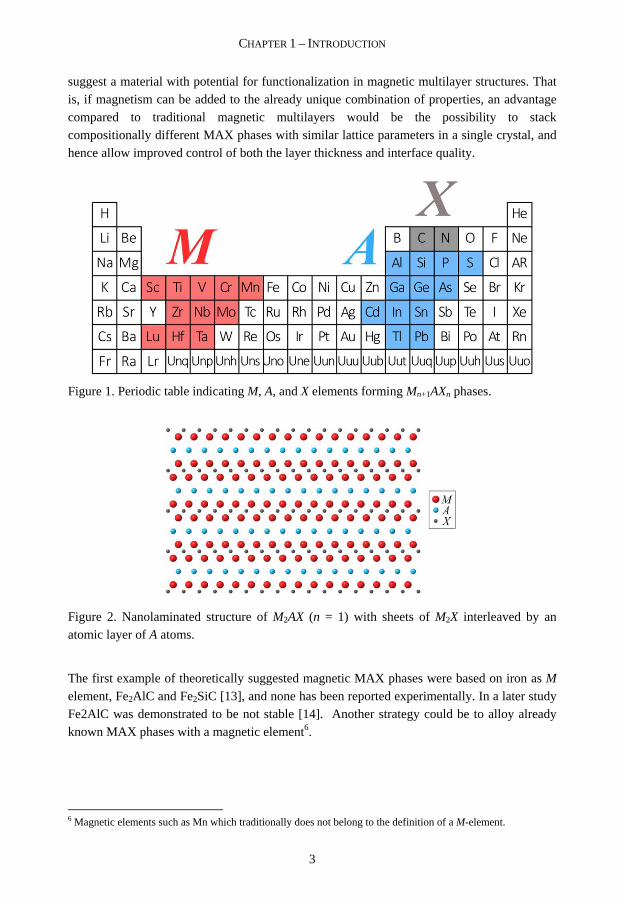
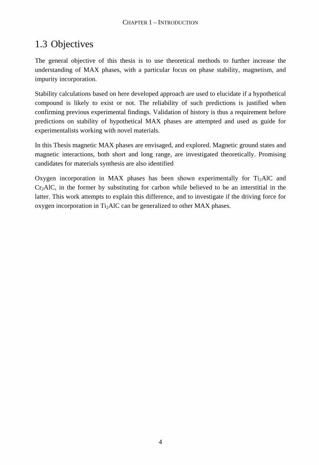
A group of nanolaminated materials that combines ceramic and metallic characteristics are the Mn+1AXn (MAX) phases, n = 1 – 3, comprised of transition metal (M) carbide or nitride (X) sheets (Mn+1Xn) interleaved by a single layer of a group 12-16 element (A) [10, 11]. The elements forming these so-called MAX phases are illustrated in Figure 1, and in Figure 2 the characteristic multilayered structure is exemplified for M2AX (n = 1). The inherently nanolaminated and highly stable structure, with suggested tunable anisotropic properties [12],
4 The term in silico refer to experiments performed on a computer such as calculations and simulations. Examples of related terms are in vivo (experiments on a living organism) and in vitro (experiments in a “test tube”, i.e. isolated from its natural surrounding). 5 In 2007, Albert Fert and Peter Grünberg were awarded the Nobel Prize in Physics for the discovery of a new physical effect known as GMR.
CHAPTER 1 – INTRODUCTION
3
suggest a material with potential for functionalization in magnetic multilayer structures. That is, if magnetism can be added to the already unique combination of properties, an advantage compared to traditional magnetic multilayers would be the possibility to stack compositionally different MAX phases with similar lattice parameters in a single crystal, and hence allow improved control of both the layer thickness and interface quality.
Figure 1. Periodic table indicating M, A, and X elements forming Mn+1AXn phases.
Figure 2. Nanolaminated structure of M2AX (n = 1) with sheets of M2X interleaved by an atomic layer of A atoms.
The first example of theoretically suggested magnetic MAX phases were based on iron as M element, Fe2AlC and Fe2SiC [13], and none has been reported experimentally. In a later study Fe2AlC was demonstrated to be not stable [14]. Another strategy could be to alloy already known MAX phases with a magnetic element6.
6 Magnetic elements such as Mn which traditionally does not belong to the definition of a M-element.
CHAPTER 1 – INTRODUCTION
4
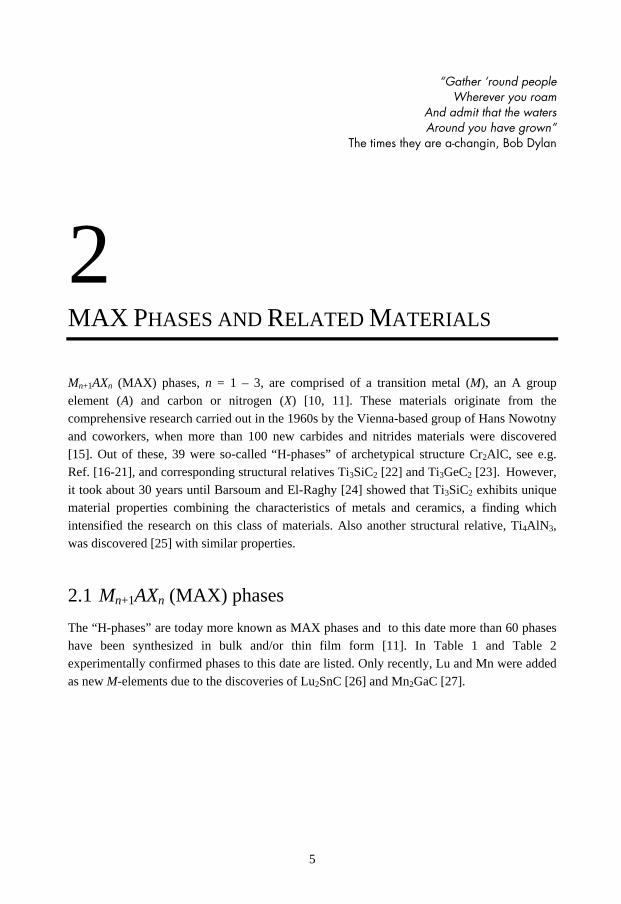
1.3 Objectives
The general objective of this thesis is to use theoretical methods to further increase the understanding of MAX phases, with a particular focus on phase stability, magnetism, and impurity incorporation.
Stability calculations based on here developed approach are used to elucidate if a hypothetical compound is likely to exist or not. The reliability of such predictions is justified when confirming previous experimental findings. Validation of history is thus a requirement before predictions on stability of hypothetical MAX phases are attempted and used as guide for experimentalists working with novel materials.
In this Thesis magnetic MAX phases are envisaged, and explored. Magnetic ground states and magnetic interactions, both short and long range, are investigated theoretically. Promising candidates for materials synthesis are also identified
Oxygen incorporation in MAX phases has been shown experimentally for Ti2AlC and Cr2AlC, in the former by substituting for carbon while believed to be an interstitial in the latter. This work attempts to explain this difference, and to investigate if the driving force for oxygen incorporation in Ti2AlC can be generalized to other MAX phases.
5
“Gather ‘round people Wherever you roam
And admit that the waters Around you have grown”
The times they are a-changin, Bob Dylan
2
MAX PHASES AND RELATED MATERIALS
Mn+1AXn (MAX) phases, n = 1 – 3, are comprised of a transition metal (M), an A group element (A) and carbon or nitrogen (X) [10, 11]. These materials originate from the comprehensive research carried out in the 1960s by the Vienna-based group of Hans Nowotny and coworkers, when more than 100 new carbides and nitrides materials were discovered [15]. Out of these, 39 were so-called “H-phases” of archetypical structure Cr2AlC, see e.g. Ref. [16-21], and corresponding structural relatives Ti3SiC2 [22] and Ti3GeC2 [23]. However, it took about 30 years until Barsoum and El-Raghy [24] showed that Ti3SiC2 exhibits unique material properties combining the characteristics of metals and ceramics, a finding which intensified the research on this class of materials. Also another structural relative, Ti4AlN3, was discovered [25] with similar properties.
2.1 Mn+1AXn (MAX) phases
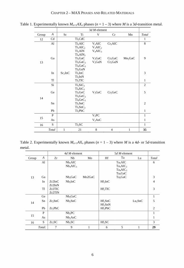
The “H-phases” are today more known as MAX phases and to this date more than 60 phases have been synthesized in bulk and/or thin film form [11]. In Table 1 and Table 2 experimentally confirmed phases to this date are listed. Only recently, Lu and Mn were added as new M-elements due to the discoveries of Lu2SnC [26] and Mn2GaC [27].
CHAPTER 2 – MAX PHASES AND RELATED MATERIALS
6
Table 1. Experimentally known Mn+1AXn phases (n = 1 – 3) where M is a 3d-transition metal.
3d M-element
Group A Sc Ti V Cr Mn Total
12 Cd Ti2CdC 1
13
Al Ti 2AlC Ti3AlC2 Ti2AlN Ti4AlN 3
V2AlC V3AlC2 V4AlC3
Cr2AlC 8
Ga Ti2GaC Ti3GaC2 Ti4GaC3 Ti2GaN
V2GaC V2GaN
Cr2GaC Cr2GaN
Mn2GaC 9
In Sc2InC Ti2InC Ti2InN
3
Tl Ti2TlC 1
14
Si Ti3SiC2 Ti4SiC3
2
Ge Ti2GeC Ti3GeC2 Ti4GeC3
V2GeC Cr2GeC 5
Sn Ti2SnC Ti3SnC2
2
Pb Ti2PbC 1
15 P V2PC 1
As V2AsC 1
16 S Ti2SC 1
Total 1 21 8 4 1 35
Table 2. Experimentally known Mn+1AXn phases (n = 1 – 3) where M is a 4d- or 5d-transition metal.
4d M-element 5d M-element
Group A Zr Nb Mo Hf Ta Lu Total
13
Al Nb2AlC Nb4AlC3
Ta2AlC Ta3AlC2 Ta4AlC3 Ta2GaC
6
Ga Nb2GaC Mo2GaC Ta2GaC 3
In Zr2InC Zr2InN
Nb2InC Hf2InC 4
Tl Zr2TlC Zr2TlN
Hf2TlC 3
14
Ge Nb2GeC 1
Sn Zr2SnC Nb2SnC Hf2SnC Hf2SnN
Lu2SnC 5
Pb Zr2PbC Hf2PbC 2
15 P Nb2PC 1
As Nb2AsC 1
16 S Zr2SC Nb2SC Hf2SC 3
Total: 7 9 1 6 5 1 29
CHAPTER 2 – MAX PHASES AND RELATED MATERIALS
7
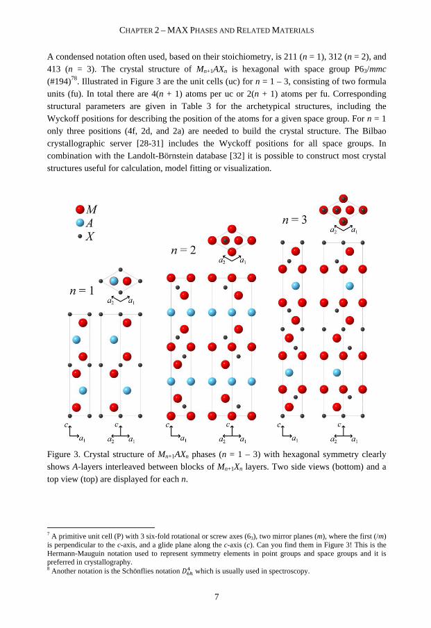
A condensed notation often used, based on their stoichiometry, is 211 (n = 1), 312 (n = 2), and 413 (n = 3). The crystal structure of Mn+1AXn is hexagonal with space group P63/mmc (#194)78. Illustrated in Figure 3 are the unit cells (uc) for n = 1 – 3, consisting of two formula units (fu). In total there are 4(n + 1) atoms per uc or 2(n + 1) atoms per fu. Corresponding structural parameters are given in Table 3 for the archetypical structures, including the Wyckoff positions for describing the position of the atoms for a given space group. For n = 1 only three positions (4f, 2d, and 2a) are needed to build the crystal structure. The Bilbao crystallographic server [28-31] includes the Wyckoff positions for all space groups. In combination with the Landolt-Börnstein database [32] it is possible to construct most crystal structures useful for calculation, model fitting or visualization.
Figure 3. Crystal structure of Mn+1AXn phases (n = 1 – 3) with hexagonal symmetry clearly shows A-layers interleaved between blocks of Mn+1Xn layers. Two side views (bottom) and a top view (top) are displayed for each n.
7 A primitive unit cell (P) with 3 six-fold rotational or screw axes (63), two mirror planes (m), where the first (/m) is perpendicular to the c-axis, and a glide plane along the c-axis (c). Can you find them in Figure 3! This is the Hermann-Mauguin notation used to represent symmetry elements in point groups and space groups and it is preferred in crystallography. 8 Another notation is the Schönflies notation ���� which is usually used in spectroscopy.
CHAPTER 2 – MAX PHASES AND RELATED MATERIALS
8
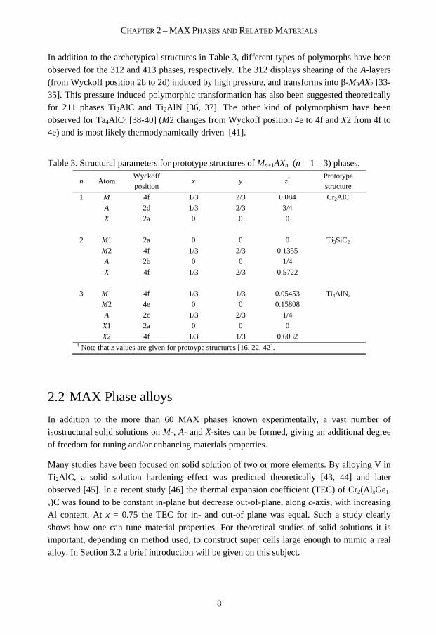
In addition to the archetypical structures in Table 3, different types of polymorphs have been observed for the 312 and 413 phases, respectively. The 312 displays shearing of the A-layers (from Wyckoff position 2b to 2d) induced by high pressure, and transforms into β-M3AX2 [33-35]. This pressure induced polymorphic transformation has also been suggested theoretically for 211 phases Ti2AlC and Ti2AlN [36, 37]. The other kind of polymorphism have been observed for Ta4AlC3 [38-40] (M2 changes from Wyckoff position 4e to 4f and X2 from 4f to 4e) and is most likely thermodynamically driven [41].
Table 3. Structural parameters for prototype structures of Mn+1AXn (n = 1 – 3) phases.
n Atom Wyckoff position
x y z† Prototype structure
1 M 4f 1/3 2/3 0.084 Cr2AlC
A 2d 1/3 2/3 3/4
X 2a 0 0 0
2 M1 2a 0 0 0 Ti3SiC2
M2 4f 1/3 2/3 0.1355
A 2b 0 0 1/4
X 4f 1/3 2/3 0.5722
3 M1 4f 1/3 1/3 0.05453 Ti4AlN 3
M2 4e 0 0 0.15808
A 2c 1/3 2/3 1/4
X1 2a 0 0 0
X2 4f 1/3 1/3 0.6032 † Note that z values are given for protoype structures [16, 22, 42].
2.2 MAX Phase alloys
In addition to the more than 60 MAX phases known experimentally, a vast number of isostructural solid solutions on M-, A- and X-sites can be formed, giving an additional degree of freedom for tuning and/or enhancing materials properties.
Many studies have been focused on solid solution of two or more elements. By alloying V in Ti2AlC, a solid solution hardening effect was predicted theoretically [43, 44] and later observed [45]. In a recent study [46] the thermal expansion coefficient (TEC) of Cr2(Al xGe1-
x)C was found to be constant in-plane but decrease out-of-plane, along c-axis, with increasing Al content. At x = 0.75 the TEC for in- and out-of plane was equal. Such a study clearly shows how one can tune material properties. For theoretical studies of solid solutions it is important, depending on method used, to construct super cells large enough to mimic a real alloy. In Section 3.2 a brief introduction will be given on this subject.
CHAPTER 2 – MAX PHASES AND RELATED MATERIALS
9
The number of X elements is by definition limited by to only C and N but due to their similar chemical bonding characteristics, resembling its binaries MC and MN, they can form a wide range of MAX carbonitride solid solutions [47, 48]. This allows investigation on correlations between chemistry and physical properties. In particular Ti2Al(C,N) solid solutions [47-52] have been extensively studied. For example, Ti2Al(C0.5N0.5) [50, 53] has been shown to be harder and stiffer than its end members, Ti2AlC and Ti2AlN.
Oxygen does not belong to the elements in the MAX phase family, as no Mn+1AOn have been synthesized. However, O can form MAX phase oxycarbides [54, 55], but not to the same extent as the carbonitrides due to reduced structural stability [56]. In Paper I of this Thesis the stability of Ti2Al(C1-xOx) was studied and predicted to be stable up to x = 0.75 [57]. In Paper II the stability concept is used for studying different types of oxygen incorporation as well as vacancy formation for M2AlC (M = Ti, V, Cr, Zr, Hf). A motivation for studies of oxygen incorporation, despite its suggested ability to tune properties [12], is that dissolution is of importance for the design of self-healing MAX phases [58-60].
MAX phase solid solutions haves been studied in several of the papers included in this Thesis. In addition to Paper I and II mentioned above, Paper VI presents theoretical predictions indicating that alloying Cr2AlC with Mn would form a stable magnetic MAX phase and allow for different magnetic ordering depending on the Cr/Mn ratio and the chemical ordering [14]. This was later experimentally realized by Mockute et al. [61]. Also (Cr,Mn)2GeC [62] and (Cr,Mn)2GaC [63] was predicted stable and later synthesized.
2.3 Related laminated materials
There are reports of phases with n ≠ 1 – 3, such as Ta6AlC5 and Ti7SnC6. However these are observed locally as irregular stackings, within Ta4AlC3 and Ti2SnC grains, with stacking sequences of a few unit cells, therefore they do not fulfill the definition of being a phase on their own [64, 65]. What does exists in sizes larger than a few unit cells are “intergrown structures” of MAX phases. First discovered by Palmquist et al. [66] was Ti5Si2C3 and Ti7Si2C5, or so called 523 and 725 phases. These can be seen as combinations of alternating half-unit cell stackings of 211 and 312 for 523, and of 312 and 413 for 725. Later the same phases were revealed also for the Ti-Ge-C [67] and Ti-Al-C [68-71] systems. In the latter system there has been a controversy weather the 523 consist of 20 atoms/uc, space group
P63/mmc (194) [70], or 30 atoms/uc, space group P3m1 (156) [68, 69] or �3�� (166) [71]. Lane et al. presented evidence from both experimental and simulated X-ray diffraction (XRD) as well as selected area electron diffraction patterns proving that the double stacking sequence of atoms is wrong; it needs to be repeated three times [68]. As a comparison, the energy difference between Mn+1AXn phases and its building blocks, MX and MA, using
CHAPTER 2 – MAX PHASES AND RELATED MATERIALS
10
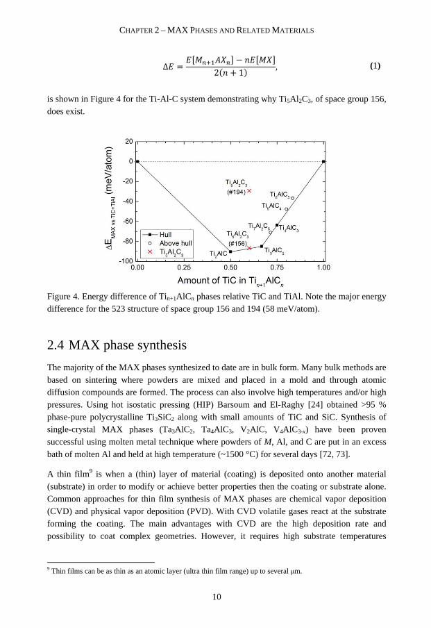
Δ = � ������� − �� ��2�� + 1� , (1)
is shown in Figure 4 for the Ti-Al-C system demonstrating why Ti5Al 2C3, of space group 156, does exist.
Figure 4. Energy difference of Tin+1AlCn phases relative TiC and TiAl. Note the major energy difference for the 523 structure of space group 156 and 194 (58 meV/atom).
2.4 MAX phase synthesis
The majority of the MAX phases synthesized to date are in bulk form. Many bulk methods are based on sintering where powders are mixed and placed in a mold and through atomic diffusion compounds are formed. The process can also involve high temperatures and/or high pressures. Using hot isostatic pressing (HIP) Barsoum and El-Raghy [24] obtained >95 % phase-pure polycrystalline Ti3SiC2 along with small amounts of TiC and SiC. Synthesis of single-crystal MAX phases (Ta3AlC2, Ta4AlC3, V2AlC, V4AlC3-x) have been proven successful using molten metal technique where powders of M, Al, and C are put in an excess bath of molten Al and held at high temperature (~1500 °C) for several days [72, 73].
A thin film9 is when a (thin) layer of material (coating) is deposited onto another material (substrate) in order to modify or achieve better properties then the coating or substrate alone. Common approaches for thin film synthesis of MAX phases are chemical vapor deposition (CVD) and physical vapor deposition (PVD). With CVD volatile gases react at the substrate forming the coating. The main advantages with CVD are the high deposition rate and possibility to coat complex geometries. However, it requires high substrate temperatures
9 Thin films can be as thin as an atomic layer (ultra thin film range) up to several µm.

CHAPTER 2 – MAX PHASES AND RELATED MATERIALS
11
(1000-1300 °C) and can involve hazardous gases. Ti3SiC2 was the first CVD made MAX phase [74].
PVD is a physical process where atoms from a solid or liquid material is sputtered or vaporized from a target, to condensate on a substrate and form a film. This has to be carried out under vacuum conditions, which provides a process with very low contamination level. PVD methods are in contrast to CVD line-of-sight methods where only the substrate surface facing the target will be coated. Much work on PVD-based thin film synthesis of MAX phases has been performed by sputtering techniques10 where the target surface is being bombarded by energetic ions, e.g. argon ions, that ejects atoms that can travel to the substrate. The target material can be either a compound [66, 75] or elemental [27, 76, 77]. The advantageous of the latter choice is a flexible individual control of the amount of material released, i.e. the elemental flux, from M, A, and X targets. The substrate is most often heated to increase the surface mobility of the arriving atoms. Typical substrate temperature are in the range 700 – 1000 °C but temperatures as low as 450 °C have been used successfully to synthesize V2GeC [78] and Cr2AlC [79]. In Paper IV and VIII, thin films of Nb2GeC and Mn2GaC were deposited by magnetron sputter epitaxy.
Another PVD technique is cathodic arc11 which operates at much higher currents as compared to sputtering techniques. At the cathode surface (target) a discharged (arc) of extremely high current density leads to erosion of molten and solid particles through micro explosions. This results in plasma of a high degree of ionization [80] that allows for control of ion energy using electric and magnetic fields, in turn to enhance control of microstructural evolution and thin film properties. The arc can be operated in a continuous direct current (DC) mode or in a pulsed mode. The latter involves much higher current and has been proven successful for MAX phase synthesis [81, 82].
10 Example of techniques used for MAX phases synthesis are magnetron sputtering, reactive magnetron sputtering which involves, e.g., N2 as a reactive gas, and high-power impulse magnetron sputtering (HIPIMS). 11 An arc is an electrical discharge with current transported through a medium normally being insulating. You may all have seen an arc in the form of lightning.


13
“The quantum world can be a touch absurd, Describable in numbers but nonsense in words,
Where waves are really particles, And particles are blurry,
What can we infer from all of this” Heisenberg’s uncertainty principle, Jonny Berliner
3
THEORETICAL METHODS
Within this chapter the tool box used during the progress leading to this thesis is introduced. A brief description is given of the theoretical framework used, density functional theory (DFT), followed by an introduction to how to model and describe configurational order/disorder in a material. Finally the linear optimization method used to investigate phase stability of Mn+1AXn phases is presented.
3.1 Density Functional Theory
In methods stated to be ab initio, meaning “from the beginning”, or from first-principles there are no empirical parameters. Instead they are directly based on quantum mechanics. The complexity encountered when treating a material quantum mechanically is the correlation between many particles. The full many-body Schrödinger equation involves 3N degrees of
freedom for N electrons, while DFT instead consider the electron density ����, as the only relevant physical quantity, only depending on 3 degrees of freedom (the position). DFT is a ground state theory which has proven to be very successful in describing structural and electronic properties for a range of materials, from atoms and molecules to simple crystals and complex extended systems. The theory is also computationally simple, which is why it has become a common tool for describing and predicting properties in condensed matter systems.
This idea of treating the particles as a function of electron density was presented in 1927 when Thomas and Fermi [83, 84] used a statistical model to approximate the distribution of electrons in an atom. However, it was not until 1964-65 that the theory to be used practically, enabled by Hohenberg, Kohn, and Sham [85, 86]. For more details on electronic structure, a book by Richard M. Martin [87] is highly recommended.

CHAPTER 3 – THEORETICAL METHODS
14
3.1.1 Hohenberg-Kohn theorems
Almost 50 years ago, in 1964, Pierre Hohenberg and Walter Kohn [85] formulated the fundament for DFT with the central idea to replace the many-body problem with an equation for the electron density. The theory consists of two theorems in which Hohenberg and Kohn stated and proved that:
Theorem 1 For any system of interacting particles in an external potential ��� �r�, the
potential ��� �r� is uniquely determined, apart from an additive constant, by knowledge of the
ground state particle density �!�rrrr�.
Theorem 2 A universal functional for the energy ��� in terms of the density ��rrrr� can be
defined, valid for any external potential ��� �r�. For any particular ��� �r�, the exact ground
state energy of the system is the global minimum value of this functional, and the density ��rrrr�
that minimizes the functional is the exact ground state density �!�rrrr�.
If the exact form of the functional ��� was known, the exact ground state density �!�rrrr� would be found and hence all ground state properties (no guidance of excited states) of the system could be completely determined. However, the explicit form of such functional is not known and approximations are needed to make use of the theory in practice.
3.1.2 Kohn-Sham equations
In 1965, Walter Kohn and Lu Jeu Sham [86] proposed an alternative approach, the Kohn-Sham ansatz, illustrated in Figure 5. The key is to substitute the real interacting system with an auxiliary system of non-interacting particles with the same density as the real system. This
is realized by letting the non-interacting particles be subject to an effective potential ��##�r�
instead of an external potential ��� �r�.
Figure 5. Schematic of the Kohn-Sham ansatz (KS) showing the connection between the many-body (left hand side) and independent-particle (right hand side) system. HK and HK0 denotes the Hohenberg-Kohn theorem applied to the many-body and non-interacting problem, respectively. After Martin [87].
The non-interacting particles are described by wavefunctions solving the single-particle Schrödinger-like equations, more known as the Kohn-Sham equations
$− 12 ∇& + ��''�(�) ϕ+��� = ε+ϕ+���,
(2)

CHAPTER 3 – THEORETICAL METHODS
15
with the effective potential given by
��##�rrrr� = ��� �rrrr� + - ��rrrr.�|rrrr----rrrr.| 1rrrr '''' + 345���rrrr��
3��rrrr� , (3)
in turn expressed by the external potential, the electron-density interaction, and the exchange-correlation function. The density of N particles is just a sum over the one-particle wave functions.
���� = 7|ϕ+���|&8
9:�. (4)
and from this the Kohn-Sham total energy functional can be derived as
<=��� = >?��� + - 1rrrr��� �rrrr���rrrr� + @AB B����� + 45��� + CC , (5)
where >?��� is the kinetic energy of the auxiliary system of non-interacting particles, ��� �r�
is the external potential, @AB B����� is the Coluomb energy for electron-electron interactions,
and CC is the energy representing interacting nuclei. Many-body effects are represented by the
exchange-correlation energy functional 45��� which cannot be calculated exactly, and as such is the only term within the Kohn-Sham approach that needs to be approximated.
3.1.3 Self-consistent solution
Based on the energy functional in Eq. (5), the total energy can be minimized to find the
ground-state energy and electron density. However, since both ��##�r� and ϕ+��� depends on
the electron density ����, an iterative process needs to be used, as illustrated in Figure 6. The
first step is to generate an initial electron density �!���, e.g. by adding single atom densities.
Next, an effective potential ��##�r� is constructed based on �!���. The third step involves
solving the Kohn-Sham equation (Eq. (2) resulting in a new set of wave functions which can
be added together using Eq. (4) to construct a new density �DE�����. To check the
convergence, a comparison of the input density �E��� with the new density �DE����� is made.
If the difference is larger than convergence value F, a new density �E����� needs to be generated, utilizing different schemes such as the Anderson method [88] or the Broyden
method [89, 90]. A new ��##�r� is then constructed and the iterative process continues until
the density has converged below F and self-consistency is reached.

CHAPTER 3 – THEORETICAL METHODS
16
Figure 6. Schematic representation of the basic steps in the Kohn-Sham self-consistent loop. After Martin [87].
3.1.4 Exchange and correlation approximations
In Eq. (5) the challenging part is the exchange-correlation energy functional 45��� which treats many-body effects. Since it is not known, approximations are needed. The first approximation was suggested in the original paper by Kohn and Sham, and was called the local density approximation (LDA) where solids are approximated as a homogenous electron gas.[86]
45GHI��� = - 1�J45�KLK����, ������. (6)
LDA works best for metals where the regions describing the bonds are far from the nuclei, and thus the electron density varies slowly. A weakness of LDA calculations is the overbinding found for many systems resulting in underestimated lattice parameters. For

CHAPTER 3 – THEORETICAL METHODS
17
systems with large density gradients, e.g. for 3d transition metals, LDA may not be suitable. An improved approximation allowing more significant non-homogeneous densities is to also
implement the effect of density gradients ∇�, like in the generalized gradient approximation (GGA),
45MMI��� = - 1�J45MMI���, ∇��, ������. (7)
There are many different GGA schemes available, e.g. those proposed by Becke (B88) [91], Perdew and Wang (PW91) [92], and by Perdew, Burke, and Ernzerhof (PBE) [93]. GGA is a better approximation as compared to LDA for many 3d transition metal systems, as the larger density gradients of the semi-core states, compared to valence state electrons, are more accurately described.
The effect of using different exchange-correlation approximations is shown in Figure 7, exemplified by M2AC MAX phase lattice parameters. The overbinding from LDA results in values of a and c to be 1.5 to 5 % below experimental values. Corresponding values from GGA calculations are within ±0.7 % of experimental ones.
Figure 7. Lattice parameters a and c for M2AC (M = Sc, Ti, V, Cr, Mn, A = Al, Ga, Ge) based on calculations using GGA (□) and LDA (○). For comparison experimental values are included (▲) [10, 17, 27, 94-96].
Even though the lattice parameters from GGA and LDA differ, the central parts of this thesis are associated with phase stability for which the energy of the phases are most important. A
CHAPTER 3 – THEORETICAL METHODS
18
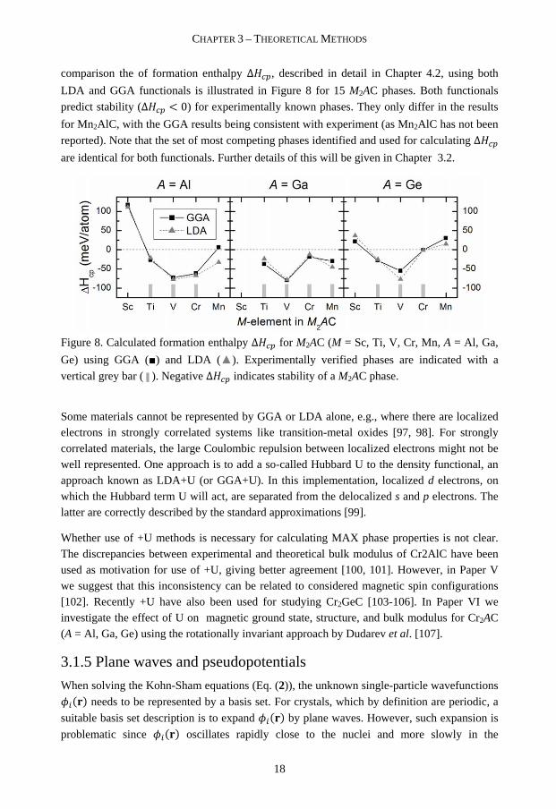
comparison the of formation enthalpy ΔNOP, described in detail in Chapter 4.2, using both
LDA and GGA functionals is illustrated in Figure 8 for 15 M2AC phases. Both functionals
predict stability (ΔNOP < 0) for experimentally known phases. They only differ in the results
for Mn2AlC, with the GGA results being consistent with experiment (as Mn2AlC has not been
reported). Note that the set of most competing phases identified and used for calculating ΔNOP
are identical for both functionals. Further details of this will be given in Chapter 3.2.
Figure 8. Calculated formation enthalpy ΔNOP for M2AC (M = Sc, Ti, V, Cr, Mn, A = Al, Ga,
Ge) using GGA (■) and LDA (▲). Experimentally verified phases are indicated with a
vertical grey bar ( ▌). Negative ΔNOP indicates stability of a M2AC phase.
Some materials cannot be represented by GGA or LDA alone, e.g., where there are localized electrons in strongly correlated systems like transition-metal oxides [97, 98]. For strongly correlated materials, the large Coulombic repulsion between localized electrons might not be well represented. One approach is to add a so-called Hubbard U to the density functional, an approach known as LDA+U (or GGA+U). In this implementation, localized d electrons, on which the Hubbard term U will act, are separated from the delocalized s and p electrons. The latter are correctly described by the standard approximations [99].
Whether use of +U methods is necessary for calculating MAX phase properties is not clear. The discrepancies between experimental and theoretical bulk modulus of Cr2AlC have been used as motivation for use of +U, giving better agreement [100, 101]. However, in Paper V we suggest that this inconsistency can be related to considered magnetic spin configurations [102]. Recently +U have also been used for studying Cr2GeC [103-106]. In Paper VI we investigate the effect of U on magnetic ground state, structure, and bulk modulus for Cr2AC (A = Al, Ga, Ge) using the rotationally invariant approach by Dudarev et al. [107].
3.1.5 Plane waves and pseudopotentials
When solving the Kohn-Sham equations (Eq. (2)), the unknown single-particle wavefunctions
S9��� needs to be represented by a basis set. For crystals, which by definition are periodic, a
suitable basis set description is to expand S9��� by plane waves. However, such expansion is
problematic since S9��� oscillates rapidly close to the nuclei and more slowly in the

CHAPTER 3 – THEORETICAL METHODS
19
interstitial regions. A huge number of plane waves with a very high cutoff energy are thus needed which limits the size of systems to be solved. Attempts to solve this are based on the approach that electrons in an atom can be categorized into:
• Core states: Localized electrons that do not take part in bonding.
• Valence states: In general non-localized electrons responsible for bonding.
• Semi-valence states: Localized electrons that do not directly contribute to bonding but may affect valence states.
In many methods, only the valence states are fully included. Depending on what properties one wants to calculate and the accuracy of the calculations, the other two states may be included as well. One example is the frozen-core approximation, where the core states are included only once, in the beginning of the calculation, as if they were in a single isolated atom. An approximation which does treat the electrons in such way is the pseudopotential method which substitutes the electron wave functions and potentials after the initial step by smooth pseudo wave functions and potentials inside a specified radius from the nucleus [87, 108]. An extension of this method is the projector augmented wave (PAW), introduced by Blöchl [109] and further developed by Kresse et al. [110]. It is an all-electron method where the wavefunctions of the core states are kept in the calculation while still applying the frozen core approximation. Thus, they are unaffected by valence states, but still available for total energy evaluations. Throughout the thesis work the PAW approach has been used as implemented within the Vienna ab-initio Simulation Package (VASP) [110, 111].
3.1.6 k-points and energy cutoff
To obtain accurate results, parameters like k-point density and plane wave cutoff energy
OT K## have to be optimized. When considering the electronic structure of a solid it is not
necessary to consider all wave vectors, only those inside the region of reciprocal space known as the first Brillouin zone (BZ)12. Due to symmetry, these can be reduced further into the irreducible Brillouin zone (IBZ), thus reducing the computational cost needed. The k-points specify points in the BZ at which plane waves are generated. More k points mean more plane waves resulting in better description of the basis set. One approach commonly used is the Monkhorst-Pack scheme [112] where the k-point density is specified in the direction of the reciprocal lattice vectors. The k-point density is inversely proportional to the corresponding unit cell vector. If a1 = a and a2 = 4a are the unit cell vectors then there should be a four times denser k-grid along reciprocal vector b1.
The cutoff energy determines the maximum energy for plane waves used in the expansions of the wavefunctions in Eq. (2) and therefore the number of plane waves in the basis set. Illustrated in Figure 9 are the total energies (left panels) and volumes (right panels) as a
12 The first Brillouin zone is the Wigner-Seitz cell of the reciprocal lattice, which is defined by the planes that are the perpendicular bisectors of the vectors from the origin of the reciprocal lattice points.
CHAPTER 3 – THEORETICAL METHODS
20
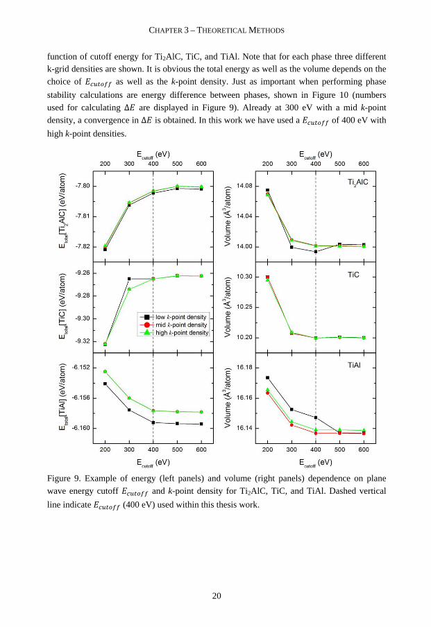
function of cutoff energy for Ti2AlC, TiC, and TiAl. Note that for each phase three different k-grid densities are shown. It is obvious the total energy as well as the volume depends on the
choice of OT K## as well as the k-point density. Just as important when performing phase
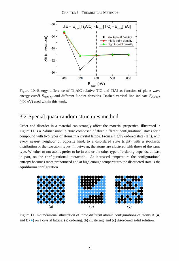
stability calculations are energy difference between phases, shown in Figure 10 (numbers
used for calculating Δ are displayed in Figure 9). Already at 300 eV with a mid k-point
density, a convergence in Δ is obtained. In this work we have used a OT K## of 400 eV with
high k-point densities.
Figure 9. Example of energy (left panels) and volume (right panels) dependence on plane
wave energy cutoff OT K## and k-point density for Ti2AlC, TiC, and TiAl. Dashed vertical
line indicate OT K## (400 eV) used within this thesis work.
CHAPTER 3 – THEORETICAL METHODS
21
Figure 10. Energy difference of Ti2AlC relative TIC and TiAl as function of plane wave
energy cutoff OT K## and different k-point densities. Dashed vertical line indicate OT K##
(400 eV) used within this work.
3.2 Special quasi-random structures method
Order and disorder in a material can strongly affect the material properties. Illustrated in Figure 11 is a 2-dimensional picture composed of three different configurational states for a compound with two types of atoms in a crystal lattice. From a highly ordered state (left), with every nearest neighbor of opposite kind, to a disordered state (right) with a stochastic distribution of the two atom types. In between, the atoms are clustered with those of the same type. Whether or not atoms prefer to be in one or the other type of ordering depends, at least in part, on the configurational interaction. At increased temperature the configurational entropy becomes more pronounced and at high enough temperatures the disordered state is the equilibrium configuration.
Figure 11. 2-dimensional illustration of three different atomic configurations of atoms A (●) and B (●) on a crystal lattice: (a) ordering, (b) clustering, and (c) disordered solid solution.

CHAPTER 3 – THEORETICAL METHODS
22
Within this work disordered states have been model by the so-called special quasi-random
structures (SQS) method, introduced by Zunger et al. [113]. Supercells are then created to mimic the atom distribution in a random alloy. The method can briefly be described as a way of creating as many nearest neighbor A-B bonds, next-nearest neighbor A-B bonds, etc., as found in a completely random alloy. Hence the method attempts to avoid ad hoc constructed supercells, which may lead to non-consistent results13.
With increasing size of the supercell, the so called Warren-Cowley SRO parameters of A- and B atoms within a sublattice can be optimized toward a random distribution of A and B. For an ideal random alloy these parameters are equal to zero [114, 115]. Hence, supercells are created to obtain short-range order (SRO) values as close to zero as possible for an increased number of shells. In Table 4 the SRO parameters are presented for Ti2Al(C1-xOx) supercells containing 32 [C+O] atoms. As the parameters are equal or close to zero for the first ten coordination shells, a random distribution of C and O on the carbon sublattice is represented..
Table 4. Short-range order (SRO) parameters for the supercells used to model different compositions of O on the carbon sublattice in Ti2Al(C1-x,Ox). The SRO parameters are given for the coordination shells of carbon, within a supercell containing 32 [C+O] atoms
Shell
x 1 2 3 4 5 6 7 8 9 10
0.25, 0.75 0.00 0.00 0.11 0.00 0.00 0.00 0.00 0.00 0.00 0.11
0.50 0.00 0.00 0.00 0.00 0.00 0.00 -0.13 0.00 -0.08 0.00
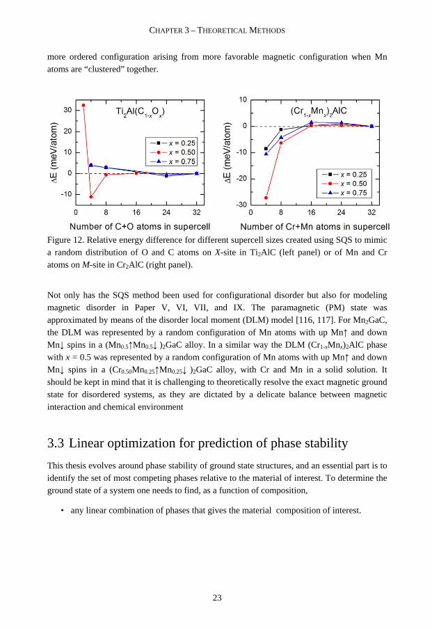
The larger the supercell used, the more correlation functions can be defined in order to mimic a random alloy. Whether a supercell can be seen as random or not in total-energy calculations is given by the nature of the effective interactions, e.g. short- or long range, in the system [114, 115]. The accuracy of using the SQS method must, as stated above, be weighed against the computational cost, and therefore supercells of different sizes should be constructed to find the limit where systems can be seen as “random”. This is illustrated in Figure 12 where the energy ∆E for different sizes of SQS generated supercells is shown relative to the energy of the largest supercell for two different systems investigated in Paper I and Paper VII. In the left panel oxygen is substituted for carbon in Ti2AlC, with cell sizes varied from 1x1x1 (two [C+O] atoms) to 4x2x2 (32 [C+O] atoms) unit cells. From 16 [C+O] atoms, ∆E is within 1 meV/atom. In the right panel Mn is alloyed with Cr2AlC forming a (Cr1-xMnx)2AlC solid solution. For all x ∆E is within 1.5 meV/atom for 16 [Cr+Mn] atoms. For both systems the largest supercell, with 32 [C+O] or [Cr+Mn] atoms have been used in this thesis work. Note the different behavior for the two systems when the supercell is constructed by a just one or a few unit cells. For [C+O] its unfavorable to be less disordered whereas Cr1-xMnx)2AlC prefer a
13 Might be difficult to distinguish a clustered, or semi-ordered, structure from a solid solution structure.
CHAPTER 3 – THEORETICAL METHODS
23
more ordered configuration arising from more favorable magnetic configuration when Mn atoms are “clustered” together.
Figure 12. Relative energy difference for different supercell sizes created using SQS to mimic a random distribution of O and C atoms on X-site in Ti2AlC (left panel) or of Mn and Cr atoms on M-site in Cr2AlC (right panel).
Not only has the SQS method been used for configurational disorder but also for modeling magnetic disorder in Paper V, VI, VII, and IX. The paramagnetic (PM) state was approximated by means of the disorder local moment (DLM) model [116, 117]. For Mn2GaC, the DLM was represented by a random configuration of Mn atoms with up Mn↑ and down Mn↓ spins in a (Mn0.5↑Mn0.5↓ )2GaC alloy. In a similar way the DLM (Cr1-xMnx)2AlC phase with x = 0.5 was represented by a random configuration of Mn atoms with up Mn↑ and down Mn↓ spins in a (Cr0.50Mn0.25↑Mn0.25↓ )2GaC alloy, with Cr and Mn in a solid solution. It should be kept in mind that it is challenging to theoretically resolve the exact magnetic ground state for disordered systems, as they are dictated by a delicate balance between magnetic interaction and chemical environment
3.3 Linear optimization for prediction of phase stability
This thesis evolves around phase stability of ground state structures, and an essential part is to identify the set of most competing phases relative to the material of interest. To determine the ground state of a system one needs to find, as a function of composition,
• any linear combination of phases that gives the material composition of interest.
CHAPTER 3 – THEORETICAL METHODS
24
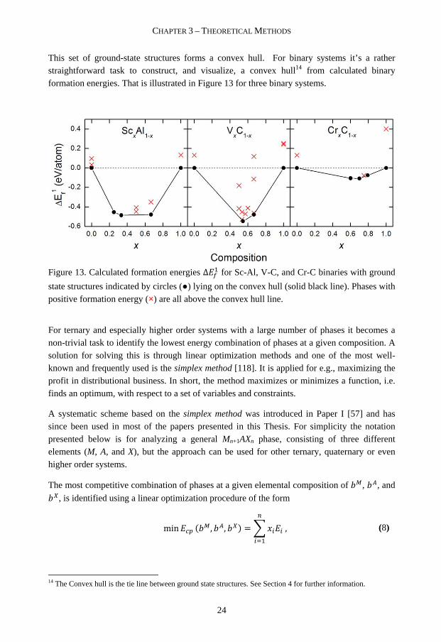
This set of ground-state structures forms a convex hull. For binary systems it’s a rather straightforward task to construct, and visualize, a convex hull14 from calculated binary formation energies. That is illustrated in Figure 13 for three binary systems.
Figure 13. Calculated formation energies ∆#� for Sc-Al, V-C, and Cr-C binaries with ground
state structures indicated by circles (●) lying on the convex hull (solid black line). Phases with positive formation energy (×) are all above the convex hull line.
For ternary and especially higher order systems with a large number of phases it becomes a non-trivial task to identify the lowest energy combination of phases at a given composition. A solution for solving this is through linear optimization methods and one of the most well-known and frequently used is the simplex method [118]. It is applied for e.g., maximizing the profit in distributional business. In short, the method maximizes or minimizes a function, i.e. finds an optimum, with respect to a set of variables and constraints.
A systematic scheme based on the simplex method was introduced in Paper I [57] and has since been used in most of the papers presented in this Thesis. For simplicity the notation presented below is for analyzing a general Mn+1AXn phase, consisting of three different elements (M, A, and X), but the approach can be used for other ternary, quaternary or even higher order systems.
The most competitive combination of phases at a given elemental composition of VW, VI, and
V4, is identified using a linear optimization procedure of the form
min OP �VW, VI, V4� = 7 [99�
9:� , (8)
14 The Convex hull is the tie line between ground state structures. See Section 4 for further information.

CHAPTER 3 – THEORETICAL METHODS
25
where [9 and 9 is the amount and energy of compound i, respectively, and OP is the energy
we want to minimize subject to the constraints
[9 ≥ 0, 7 [9W = VW�
9:�, 7 [9I = VI
�
9:�, 7 [94 = V4
�
9:�. (9)
For Mn+1AXn phases the constraints are
VW = � + 1
VI = 1
V4 = �.
(10)
Using Eq. (8) it is thus possible to find the combination of phases which has the lowest total energy at the Mn+1AXn composition. The resulting formation enthalpy is thereafter calculated according to
∆NOP� ������� = � ������� − min OP �VW, VI, V4� (11)
where � ������� is the calculated total energy of the Mn+1AXn phase and OP comes from
solving Eq. (8). For a negative value of ∆NOP the phase is stable, whereas a positive value
indicates that the phase is not stable or at best metastable.
Illustrated in Figure 14 is a schematic flow chart summarizing the linear optimization procedure used to identify the set of most competitive phases at a given composition.
Figure 14. Schematic flow chart of how to calculate the formation enthalpy.

27
“I'll make your visions sing I'll open endless skies
And ride your broken wings Welcome to my world”
Welcome to my world, Depeche Mode
4
MAX PHASE STABILITY
Bonds between constituent atoms of any molecule or solid can briefly be described as a way of redistributing valence electrons in order to make the resulting structure energetically favorable. To which extent depends not only on the internal energy (E), but also on the environment (temperature T, pressure p, competing phases, etc.). This is taken into consideration in the free energy [119]
] = + ^� − >_. (12)
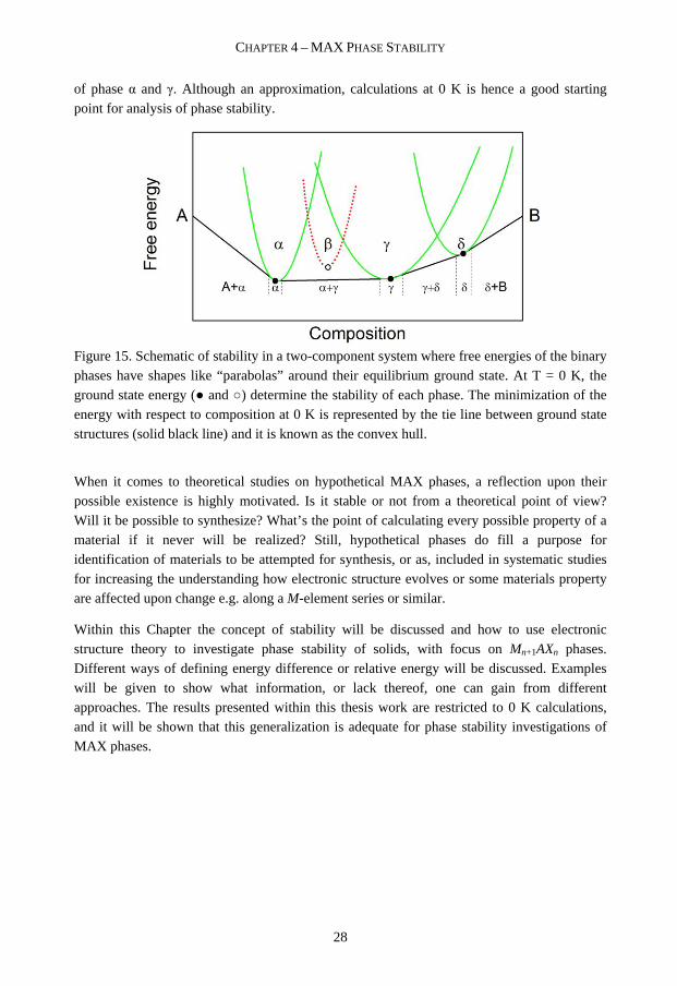
where V is the volume and S the entropy. At finite temperatures (T > 0 K), the entropy S contributes to the free energy. Entropy is a measure of disorder. Hence the term –TS in the free energy favors disordered phases and their presence increases with T. At low temperatures, low energy excitations such as geometrical distortions determine the behavior of a system. In principle the free energy of a phase can be approximated with its ground state energy. This might be understood by the free energy having the shape of a “parabola” centered on the ground state energy and concentrations, as illustrated in Figure 15. As such, knowledge of the ground state energy is often a good approximation for evaluating the phase stability at low temperatures,. The set of tie lines that connects the structures of lowest energy for various composition, (●) in Figure 15, is called the convex hull and it represents the energy of the alloy at T = 0 K. Structures above the tie line are not stable with respect to the mixture of the two structures that defines the vertices of the tie line. This is exemplified in Figure 15 by the phase β (○) being unfavorable or metastable15 with respect to a combination 15 A system, here phase β, in a local, but not a global, free energy minimum is dented as metastable. The existence of a free energy barrier between the metastable and globally stable state of the system allows the metastable state to exist.
CHAPTER 4 – MAX PHASE STABILITY
28
of phase α and γ. Although an approximation, calculations at 0 K is hence a good starting point for analysis of phase stability.
Figure 15. Schematic of stability in a two-component system where free energies of the binary phases have shapes like “parabolas” around their equilibrium ground state. At T = 0 K, the ground state energy (● and ○) determine the stability of each phase. The minimization of the energy with respect to composition at 0 K is represented by the tie line between ground state structures (solid black line) and it is known as the convex hull.
When it comes to theoretical studies on hypothetical MAX phases, a reflection upon their possible existence is highly motivated. Is it stable or not from a theoretical point of view? Will it be possible to synthesize? What’s the point of calculating every possible property of a material if it never will be realized? Still, hypothetical phases do fill a purpose for identification of materials to be attempted for synthesis, or as, included in systematic studies for increasing the understanding how electronic structure evolves or some materials property are affected upon change e.g. along a M-element series or similar.
Within this Chapter the concept of stability will be discussed and how to use electronic structure theory to investigate phase stability of solids, with focus on Mn+1AXn phases. Different ways of defining energy difference or relative energy will be discussed. Examples will be given to show what information, or lack thereof, one can gain from different approaches. The results presented within this thesis work are restricted to 0 K calculations, and it will be shown that this generalization is adequate for phase stability investigations of MAX phases.
CHAPTER 4 – MAX PHASE STABILITY
29
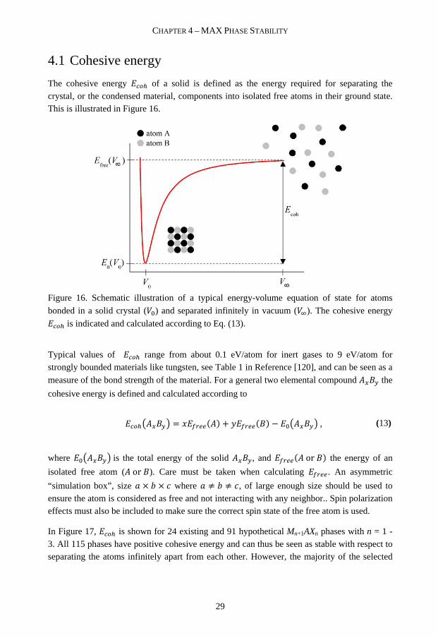
4.1 Cohesive energy
The cohesive energy OK� of a solid is defined as the energy required for separating the crystal, or the condensed material, components into isolated free atoms in their ground state. This is illustrated in Figure 16.
Figure 16. Schematic illustration of a typical energy-volume equation of state for atoms
bonded in a solid crystal (�!) and separated infinitely in vacuum (�̀ ). The cohesive energy
OK� is indicated and calculated according to Eq. (13).
Typical values of OK� range from about 0.1 eV/atom for inert gases to 9 eV/atom for strongly bounded materials like tungsten, see Table 1 in Reference [120], and can be seen as a
measure of the bond strength of the material. For a general two elemental compound ��ab the
cohesive energy is defined and calculated according to
OK�c��abd = [#B����� + e#B���a� − !c��abd , (13)
where !c��abd is the total energy of the solid ��ab, and #B���� or a� the energy of an
isolated free atom (� or a). Care must be taken when calculating #B��. An asymmetric
“simulation box”, size g × V × i where g ≠ V ≠ i, of large enough size should be used to ensure the atom is considered as free and not interacting with any neighbor.. Spin polarization effects must also be included to make sure the correct spin state of the free atom is used.
In Figure 17, OK� is shown for 24 existing and 91 hypothetical Mn+1AXn phases with n = 1 - 3. All 115 phases have positive cohesive energy and can thus be seen as stable with respect to separating the atoms infinitely apart from each other. However, the majority of the selected

CHAPTER 4 – MAX PHASE STABILITY
30
phases have not yet been synthesized, or at least not reported, although attempts have been made in the quest for, e.g., Ti2SiC16 [11, 121].
Figure 17. Calculated cohesive energy OK� for known and hypothetical Mn+1AXn phases. Note that series with A = Al and Ge overlap.
The example above was shown to point out that cohesive energy by itself may not be of overriding importance for the stability, i.e. existence, of a phase. This will be further discussed below.
4.2 Formation energy
For a compound to be stable, it must not only be more stable than its constituent free atoms, but also stable with respect to its constituent atoms in their ground-state crystal structure. The
concept of formation energy ∆#� for Mn+1AXn phases is defined by
∆#�� ������� = !� ������� − �� + 1�!� � − !��� − �!���2�n+1� , (14)
where !�k� expresses the total energy per formula unit of phase Z. ∆#� determines if the
considered phase is stable (< 0) or not (> 0).17 Shown in Figure 18 are calculated ∆#� for 115
considered Mn+1AXn phases (n = 1 - 3). Note that stability is indicated for a positive value of 16 Note that among the 39 M2AX phases Ti2SiC was found with highest cohesive energy. 17 Note that Eq. (13) and (14) are defined in different order hence the positive and mostly negative values in Figure 17 and Figure 18 , respectively.

CHAPTER 4 – MAX PHASE STABILITY
31
the cohesive energy OK�, and for a negative value of ∆#�, due to the choice of definition for
the cohesive energy (Eq. (13)). Also note that the numbers have almost decreased by an order
of magnitude as compared to OK� in Figure 17 , due to subtraction between two large, almost equal, numbers. The Mn+1ACn phases display a clear minimum, indicating maximum stability,
at M = Ti (see corresponding maxima Figure 17). M > Ti, there is an increase in ∆#�, i.e. a
decreased stability. This result is in agreement with studies for MC, NaCl-struture, and is suggested to be due to band-filling of bonding M d – C p hybridized states [122, 123]. As more d-electrons are added, nonbonding and antibonding states are gradually populated causing a decreased stability. For N-based MAX phases this minimum is slightly shifted to
the left (M ≤ Sc). Since N has one more valence electron as compared to C, bands are filled earlier in the M-series. The kink observed around M = Mn is related to magnetism stabilizing the Mn+1AXn phases.
109 phases seem to be stable in terms of ∆#� < 0, which is far from the 24 phases known
experimentally. It becomes obvious that ∆#� alone is an insufficient parameter in evaluating
stability of Mn+1AXn phases.
Figure 18. Formation energy ∆#� for Mn+1AXn phases (with n = 1 – 3) relative its constituent
elements in their ground-state crystal structure.
For more reliable phase stability calculations, competing phases including constituent atoms in their ground-state crystal structure as well as binary and ternary phases need to be included. To emphasize that a phase is fully relaxed the calculated equilibrium total energy is denoted
!. This notation can be related to the enthalpy N = ! − ^�, where ̂ is the pressure and �

CHAPTER 4 – MAX PHASE STABILITY
32
the volume of the system. For fully relaxed phases ^ = 0 and hence N = !. For Mn+1AXn the energy difference with respect to competing phases is then here defined as the formation enthalpy per atom as given by
∆N� ������� = !� ������� − !�competing phases�2�n+1� , (15)
where !� ������� is the total energy of Mn+1AXn, and !�competing phases� the total
energy for a set of competing phases with of total stoichiometry equal to ������.
In the literature there are studies where stability of MAX phases have been investigated, including binaries as well as ternaries, as competing phases. [13, 66, 124-126] In accordance
with experiments Palmquist et al. [66] do find Ti4SiC3 as theoretically stable (∆N = -29
meV/atom). However, also Ti2SiC was predicted stable (∆N = -8 meV/atom) albeit its existence has not yet been reported [11]. Fang et al. [124] predicted the so far non-existing Ti2SiC to be stable (-50 meV/atom) and the existing Ti3SiC2 to not be stable (+3 meV/atom). One of the reasons for these discrepancies were the assumption of x = 0 in Ti5S3Cx in the latter study. In a later study the inclusion of Ti5S3Cx with x = 1 reveled Ti2SiC as not stable (+4 meV/atom), in accordance with phases like M5Si3Cx (M = Ti, V, Nb), which are known to be stabilized upon incorporation of carbon [127, 128]. Other examples are evaluation of stability of V2SiC (-68 meV/atom), V3SiC2 (+2 meV/atom), and Nb3SiC2 (+20 meV/Atom).
The most ambitious study concerning stability calculations of Mn+1AXn, excluding this work, is by Keast et al. [126] investigating five ternary systems (M = Ti and Cr, A = Al and Si, X = C and N). The overall result matches experimental observations very well, although the set of most competitive phases was not identified for some MAX phases. This is exemplified in Table 5 for Ti2AlC and Ti3AlC2, where the competing phases used in Ref [126] are compared to those identified using linear optimization (see Section 3.3) . Even though Ti2AlC and
Ti3AlC2 are stable with both sets of competing phases, the values of ∆N differ significantly
Table 5. Calculated ∆N from different ways of choosing competing phases based on data from Table 3 in Keast et al [126].
Choice of competing phases ∆N (meV/atom)
Ti2AlC Ti3AlC2
by-hand [126] -91
Ti3AlC, TiC, TiAl -22
Ti2AlC, TiC
use of linear optimization -51
Ti3AlC2, TiAl -14
Ti2AlC, Ti4AlC3
Table 5 illustrates the difficulties associated with identifying the set of most competitive phases by-hand. If investigating, e.g., a quaternary compound with 30 competing, the complexity increases. Therefore, use of linear optimization is an excellent tool for identification of the most competitive set of competing phases and hence avoid ad-hoc choices.

CHAPTER 4 – MAX PHASE STABILITY
33
Another important issue to take into consideration is what competing phases to include in the phase stability calculations. In Ref. [124] Fang et al. comments on the ambiguity of selecting competing phases in the ternary phase diagram. The few stability studies of MAX phases reported [13, 66, 124-126] make use of experimental ternary phase diagrams, with focus on tie lines and three-phase regions. However, to include all phases careful investigations of the phase diagrams are necessary to elucidate candidates. Low-temperature structures should be included, as these may be the ones of lowest energy, but also structures at higher temperature may be included. Binaries are often well-explored with known structures and compositions over a large temperature span. For ternary and higher-order compounds the larger “phase space”18 often results in phase diagrams at a selected fixed temperature. Hypothetical phases should also be considered, based on known compounds in neighboring or similar systems to the one investigated. One example is the inverse perovskite19 M3AX, based on the mineral perovskite20 CaTiO3, experimentally known in some MAX phase related systems (e.g. Sc3AlN [129, 130], Sc3InC [131], Ti3AlC [132], Nb3GeC [133]). In the Ti-Al-N system two versions of the Ti3AlN perovskite are reported - the cubic inverse perovskite [134] and a distorted perovskite of orthorhombic structure (filled Re3B-type) [48].
When one or several phases are not included in the identification of the set of most competitive competing phases the corresponding formation enthalpy represents a lower energy boundary. This might be pushed to higher values if competitive phases are included.
As a consequence the values of ∆N can always become less negative or more positive.
The working process used throughout this work for phase stability calculations is illustrated in Figure 19. All issues discussed above are relevant in the second step of the figure.
Figure 19. Schematic work process used for phase stability calculations.
18 In this context ”phase space” is related to temperature range and the compositional combinations. 19 Space group u�3�� (#221). 20 Named after a Russian mineralogist, Count Lev Aleksevich von Perovski, and was discovered and named by Gustav Rose in 1839 from samples found in the Ural Mountains.
CHAPTER 4 – MAX PHASE STABILITY
34
4.3 Validation of theoretical approach
Within this section the phase stability will be presented for experimentally known and hypothetical carbide- and nitride-based Mn+1AlXn (n = 1 – 3) with M = Sc, Ti, V, Cr, Mn, Fe, and Co. The choice of A = Al is motivated by the comparatively large number of known MAX phases with this element. The results were first presented in Paper III and later extended in Paper VI. Since then, a few new competing phases has been included, e.g. Ti5Al 2C3, based on recent discoveries [69-71]. The results presented here do include these in the analysis. For each of the 11 ternary systems, including 36 MAX phases in total, careful investigations of phase diagrams and experimental works have been conducted in order to avoid ad hoc choices of competing phases, see e.g. Refs. [32, 135].
Table 6 lists competing phases included in the investigation.. For Cr-, Mn-, Fe-, and Co-based compounds different magnetic configurations were tested and the one with lowest energy, considered as the magnetic ground-state, was included in the analysis as a competing phase. For each of the 36 MAX phases, the simplex method was used to solve the linear optimization problem and consequently identify the set of most competitive competing phases, see Table 5.
Corresponding formation enthalpy ∆NOP is calculated using Eq. (15) and listed in Table 7.
The calculated formation enthalpies are also displayed in Figure 20, showing minimum values
of ∆NOP, or maximum stability, around M = V for C-based phases and at M = Ti for N-based
phases. The explanation for this behavior can be related to the number of valence electrons with N having one more valence electron compared to C and hence bands are filled earlier in the M-series. Similar trends were also found for the formation energies in Figure 18. Another observation is the slight shift of these minima’s to the left as n increase.

CHAPTER 4 – MAX PHASE STABILITY
35
Table 6. Competing phases included for M-Al-X systems. Notation within parenthesis is the crystal structure used for corresponding phase as given by the Pearson symbol21. For Cr-, Mn-, Fe-, and Co-based compounds different magnetic configurations were tested.
Single elements
Sc (hP2, hP6, tP4), Ti (cF4, cI2, hP2), V (cF4, cI2, hP2), Cr (cF4, cI2, hP2), Mn (cI58, cP2, cP20, tP4), Fe (cF4, cI2), Co (cF4, cI2, hP2), Al (cF4, cI2, hP4), C (cF8, hP4) N as N2
Binary and ternary phases
Al 4C3 (hR21), AlN (cF8, hP4)
Sc2Al (hP6), ScAl (cP2, oC8), ScAl2 (cF24), ScAl3 (cP4), Sc2C (hP3), Sc4C3 (cI28), ScC (cF8), ScC0.875 (cF8), Sc3C4 (tP70), Sc2AlC (hP8), Sc3AlC2 (hP12), Sc4AlC3 (hP16), ScAl3C3 (hP14), Sc3AlC (cP5), ScN (cF8), ScN0.875 (cF8), Sc2AlN (hP8), Sc3AlN 2 (hP12), Sc4AlN 3 (hP16), Sc3AlN (cP5)
Ti3Al (hP8), TiAl (tP4), TiAl2 (tI24), TiAl3 (tI8), Ti2C (cF48), TiC (cF8, hP4), TiC0.875 (cF8), TiC0.75 (cF8), Ti2AlC (hP8), Ti3AlC2 (hP12), Ti4AlC3 (hP16), Ti12Al 3C8 (hP46), Ti5AlC4 (hP20), Ti6AlC5 (hP24), Ti5Al 2C3 (hP20, hP30), Ti7Al 2C5 (hP42), Ti3AlC (cP5, oP20), Ti2N (tP6), TiN (cF8), TiN0.875 (cF8), Ti2AlN (hP8), Ti3AlN 2 (hP12), Ti4AlN 3 (hP16), Ti5AlN 4 (hP20), Ti6AlN 5 (hP24), Ti3AlN (cP5, oP20)
V3Al (cP8), V5Al 8 (cI52), VAl3 (tI8), V3Al 10 (cI52), V7Al 45 (mC104), VAl10 (cF176), V2C (hP3, oP12), VC0.5 (hP4),VC0.67 (hR24), V4C3 (hP21), V6C5 (hP33), V8C7 (cP60), VC (cF8, hP4), VC0.875 (cF8), V2AlC (hP8), V3AlC2 (hP12), V4AlC3 (hP16), V12Al3C8 (hP46), V5Al 2C3 (hP20, hP30), V7Al 2C5 (hP42), V3AlC (cP5), V2N (hP9), VN (cF8), VN0.875 (cF8), V2AlN (hP8), V3AlN 2 (hP12), V4AlN 3 (hP16), V3AlN (cP5)
Cr2Al ( tI6), Cr5Al 8 (cI52), Cr4Al 9 (hR26), Cr5Al 21 (hR26), Cr7Al 43 (mC104), Cr23C6 (cF116), Cr3C (oP16), Cr7C3 (hP20, oP40), Cr3C2 (oP20), Cr2AlC (hP8), Cr3AlC2 (hP12), Cr4AlC3 (hP16), Cr3AlC (cP5), Cr2N (hP9), CrN (cF8, oP8) CrN0.875 (cF8), Cr2AlN (hP8), Cr3AlN 2 (hP12), Cr4AlN 3 (hP16), Cr3AlN (cP5)
Mn3Al (cP20), Mn7Al 3 (cP20), MnAl (cP2, tP2, tP4), Mn4Al 11 (aP15), Mn3Al 10 (hP26), MnAl6 (oS28), Mn23C6 (cF116), Mn3C (oP16), Mn5C2 (mS28), Mn7C3 (hP20, oP40), MnC (hP4), Mn2AlC (hP8), Mn3AlC2 (hP12), Mn4AlC3 (hP16), Mn3AlC (cP5), Mn4N (cP5), Mn2N (hP3, hP4), Mn3N2 (tI10), MnN (cF8) MnN0.875 (cF8), Mn2AlN (hP8), Mn3AlN 2 (hP12), Mn4AlN 3 (hP16), Mn3AlN (cP5)
Fe3Al (cP4, cF16), FeAl (cP2), Fe5Al 8 (cI52), Fe3C (cP5, oP16, hP8), Fe5C2 (mS28), Fe2C (hP6, oP6), Fe2AlC (hP8), Fe3AlC2 (hP12), Fe4AlC3 (hP16), Fe3AlC (cP5)
Co3Al (cP4), CoAl0.875 (cP2), CoAl (cP2), Co2Al 5 (hP28), CoAl3 (cP4), Co2Al 9 (mP22), Co2AlC (hP8), Co3AlC2 (hP12), Co4AlC3 (hP16), Co3AlC (cP5)
21 The Pearson symbol is used to describe the crystal structure and consists of two letters specifying one of the fourteen Bravais lattices followed by a number giving the number of atoms in the unit cell. Lower case letter specify the crystal class: a (triclinic), m (monoclinic, o (orthorhombic), t (tetragonal), h (hexagonal or rhombohedral, c (cubic). Upper case letters specify the lattice type: P (primitive), F (all face centered), I (body centered), R (rhombohedral), and S,A,B,C (side face centered).

CHAPTER 4 – MAX PHASE STABILITY
36
Table 7. Identified set of most competing phases and corresponding formation enthalpy ∆NOP
for Mn+1AlXn phases (n = 1 – 3). For clearness phases with ∆NOP < 0, i.e. being stable, are
marked as bold. Mn+1ACn Mn+1ANn
M n Most competing phases ∆NOP
(meV/atom) Most competing phases
∆NOP
(meV/atom)
Sc
1 Sc3AlC, ScAl3C3 117 ScN, ScAl2, Sc3AlN 88
2 Sc3AlC, Sc3C4, ScAl3C3 155 ScN, ScAl2, Sc3AlN 36
3 Sc3AlC, Sc3C4, ScAl3C3 191 ScN, ScAl2, Sc3AlN 20
Ti
1 TiAl, Ti5Al 2C3 (hP30) -18 Ti3AlN 2, TiAl 2, Ti3AlN (oP20) -50
2 Ti5Al 2C3 (hP30), Ti7Al 2C5 -6 Ti2AlN, Ti 4AlN 3 13
3 Ti3AlC2, TiC 0 Ti2AlN, Ti 6AlN 5 -15
V
1 V5Al 2C3 (hP30), V3Al, VAl 3 -50 V2N, VAl3, AlN 15
2 V2AlC, V6C5, Al4C3 -5 V2N, AlN, VAl 3 154
3 V3AlC2, V6C5, Al4C3 6† V2N, AlN 204
Cr
1 Cr2Al, Cr3C2, Al4C3 -62 Cr (cI2), AlN 353
2 Cr2AlC, Cr3C2, C (hP4) 81 Cr (cI2), Cr2N, AlN 324
3 Cr2AlC, Cr3C2, C (hP4) 108 Cr2N, AlN 306
Mn
1 Mn3AlC, MnAl, C (hP4) 6 Mn (cI58), AlN 380
2 Mn3AlC, C (hP4) 95 Mn2N, Mn4N, AlN 363
3 Mn3AlC, C (hP4), Mn23C6 155 Mn2N, AlN 311
1 Fe3AlC, C (hP4), Fe5Al 8 78
Fe 2 Fe3AlC, C (hP4) 258
3 C (hP4), Fe3AlC, Fe (cI2) 349
1 Co (hP2), C (hP4), CoAl 255
Co 2 Co (hP2), C (hP4), CoAl 395
3 Co (hP2), C (hP4), CoAl 490 † ∆NOP = -12 meV/atom with 11 % ordered vacancies on the carbon sublattice in a V12Al 3C8 structure (hP46)
(more specific, 1/3 of C atoms in Wyckoff position 2a are empty). Experimentally observed by Etzkorn et al. [72].
Figure 20. Calculated formation enthalpy ∆NOPfor Mn+1AlXn phases (n = 1 – 3) relative to the
identified set of most competing phases listed in Table 7.
CHAPTER 4 – MAX PHASE STABILITY
37
Table 8 shows experimentally known MAX phases in relation to those calculated with
negative formation enthalpy (∆NOP < 0). Hence, the theoretical results are consistent with
existing as well as non-existing (hypothetical) Mn+1AlXn phases. This study can be seen as a benchmark, demonstrating that the theoretical method used is a useful tool to be used as guidance in the search for new Mn+1AXn phases. The method may also be applicable to other complex ternary or higher-order materials systems. It should be stressed that even though this approach does not consider entropy or other temperature related effects, the excellent correspondence with experimental findings indicates that formation of Mn+1AXn phases are
mainly governed by the total energy term in the Gibbs free energy ]. A recent investigation of Tin+1AlCn stability at finite temperatures, also including effects from lattice vibrations
(phonons), thermal expansion, and electronic excitation into ], shows that the total energy (at
0 K) is the most important parameter, whereas other contributions almost cancel out in ∆] [136].
Table 8. Calculated Mn+1AlXn phases with negative formation enthalpy (∆NOP < 0) compared
to experimentally known MAX phases for the here investigated ternary systems.
Phases with ∆NOP < 0 [137] Phases known experimentally [11]
Ti2AlC, Ti3AlC2, Ti4AlC3† Ti2AlC, Ti3AlC2
V2AlC, V3AlC2, V4AlC3‡ V2AlC, V3AlC2, V4AlC3
‡
Cr2AlC Cr2AlC
Ti2AlN, Ti 4AlN 3 Ti2AlN, Ti 4AlN 3
† ∆NOP = 0.0 meV/atom to the level of accuracy of our work.
‡ 11% (or 1/9th) ordered carbon vacancies stabilize V4AlC3 in a V12Al 3C8 structure (hP46). Experimentally observed by Etzkorn et al. [72].
4.4 Prediction of new MAX phases
Within this section the predictive power of our theoretical approach for phase stability investigations will be demonstrated for two different material systems. The results are based on Paper IV and VIII.
4.4.1 Nb2GeC
One of the first materials investigated were Nbn+1GeCn phases (n = 1 – 3). This hypothetical material was selected based on two criteria; (i) at the time no Nbn+1GeCn was known and (ii) the material was suggested to be superconducting. In Table 9 are the complete list of included competing phases with corresponding calculated energy and structural parameters. The set of most competitive phases at compositions corresponding to n = 1 – 3 was identified through use of the linear optimization procedure. Only Nb2GeC was found to be stable (-18 meV/atom) with NbGe2, Nb6C5, and Nb5Ge3C as set of most competitive phase. Nb3GeC2 and Nb4GeC3 are not stable relative to a combination of Nb2GeC, Nb6C5, and C.

CHAPTER 4 – MAX PHASE STABILITY
38
Table 9. Competing phases included in the Nb-Ge-C system with calculated total energies E0 and lattice parameters. Based on Supplemental material in Ref. [77].
Phase Prototype Pearson symbol
a (Å) b (Å) c (Å) E0
(eV/f.u.) Note
Nb W cI2 3.322 -10.092
Ge C cF8 2.881 -4.622 diamond structure
C C hP4 2.464 7.250 -9.225 graphite structure
NbC NaCl cF8 4.508 -20.249
NbC0.875 NaCl cF8 4.490 -19.076 4b-site partially occupied by C
Nb6C5 V6C5 mC22 5.523 9.541 5.510 -112.773 β = 109.6°
Nb2C Fe2N hP9 5.455 4.979 -30.799
Nb2C MoO2 oP12 11.017 3.111 5.000 -30.831
NbC0.5 NiAs hP12 3.173 4.961 -30.815 2a-site partially occupied by C
NbGe2 CrSi2 hP9 5.015 6.840 -20.366
Nb3Ge Cr3Si cP8 5.183 -36.000
Nb5Ge4 Mn5Si3 hP18 8.027 5.436 -72.657 2b-site fully occupied by Ge
Nb5Ge3.5 Mn5Si3 hP68 7.857 5.429 -70.565 2b-site partially occupied by Ge
Nb5Ge3Cx Mn5Si3 hP16 7.717 5.351 -67.680 x = 0.0
Nb5Ge3Cx Mn5Si3 hP34 7.724 5.352 -73.507 x = 0.5 (2b-site partially occupied by C)
Nb5Ge3Cx Mn5Si3 hP18 7.664 5.531 -78.330 x = 1.0 (2b-site fully occupied by C)
Nb5Ge3 W5Si3 tI32 14.399 14.530 5.202 -68.078
Nb3GeC CaTiO3 cP5 4.300 -44.537 inverse perovskite
Nb3GeC Re3B oP20 3.347 10.662 8.422 -46.835 distorted perovskite
Nb2GeC Cr2AlC hP8 3.265 12.655 -36.100 211 MAX phase
Nb3GeC2 Ti3SiC2 hP12 3.179 18.556 -56.274 312 MAX phase
Nb4GeC3 Ti4AlN 3 hP16 3.196 23.616 -76.650 413 MAX phase
Table 10. Calculate formation enthalpy ∆NOP for Nbn+1GeCn phases using Eq. (11) and
corresponding identified set of most competitive phases.
n ∆NOP (meV/atom) Most competing phases
1 -18 NbGe2, Nb6C5, Nb5Ge3Cx (x = 1.0)
2 +26 Nb2GeC, Nb6C5, C
3 +14 Nb2GeC, Nb6C5, C
Based on the prediction that Nb2GeC is stable, experimental synthesize Nb2GeC thin films by dc magnetron sputtering were initiated. Experimental details and results from characterization are given in Ref. [77]. The former hypothetical Nb2GeC was predicted stable, was successfully synthesized, and a new MAX22 phase was born.
22 Note that Nb2GeC was the first M2AX (n = 1) to be made since the 1960s (not considering alloyed combinations).

CHAPTER 4 – MAX PHASE STABILITY
39
4.4.2 Mn2GaC
Confident by the results from theoretical validation of already existing phases (Paper III), the successful prediction of a new MAX phase in Paper IV (Nb2GeC), and the first magnetic MAX upon alloying Cr2AlC with Mn (Paper VII), Mn+1GaCn phases (M = Ti, V, Cr, Mn, and n = 1 -3) were selected for phase stability investigation based on two criteria;
(i) Ga is directly below Al in the periodic table with several experimentally known MAX phases (Ti2GaC, Ti3GaC2, Ti4GaC3, V2GaC, and Cr2GaC).
(ii) Can Mnn+1GaCn be stable (Mn2AlC close to stable in Paper III)?
Careful investigations of phase diagrams and experimental works have been conducted in order to avoid ad hoc choices of competing phases, see e.g. Refs. [32, 135] and Table 11 display included competing phases. For all Cr- and Mn-based compounds nonmagnetic (NM), ferromagnetic (FM), and different antiferromagnetic (AFM) states were tested and the configuration with lowest energy, representing the magnetic ground-state, was included in the study. More details of the magnetic states for MAX phases will be given in Chapter 5. Based on the calculated total energy the set of most competing phases was identified, see Table 12, by solving the linear optimization problem.
Table 11. Competing phases included for M-Ga-C systems. Notation within parenthesis is the crystal structure used for corresponding phase as given by the Pearson symbol. For Cr- and Mn-based compounds different magnetic configurations were tested.
Single elements
Ti (cF4, cI2, hP2), V (cF4, cI2, hP2), Cr (cF4, cI2, hP2), Mn (cI58, cP2, cP20, tP4), Ga (oC4, oC8, mC4), C (cF8, hP4)
Binary and ternary phases
Ti0.9Ga0.1 (hP2), Ti0.875Ga0.125 (hP2), Ti3Ga (hP8), Ti2Ga (hP6), Ti5Ga3 (hP16, tP32, tI32), Ti5Ga4 (hP18), TiGa (tP4), Ti2Ga3 (tP10), Ti3Ga5 (oC16, tP32), TiGa2 (tI24), TiGa3 (tI8), Ti2C (cF48), TiC (cF8, hP4), TiC0.875 (cF8), TiC0.75 (cF8), Ti2GaC (hP8), Ti3GaC2 (hP12), Ti4GaC3 (hP16), Ti3GaC (cP5, oP20)
V3Ga (cP8), V6Ga5 (hP22), V6Ga7 (cI52), V2Ga5 (tP14), V8Ga41 (hR147), V2C (hP3, oP12), VC0.5 (hP4),VC0.67 (hR24), V4C3 (hP21), V6C5 (hP33), V8C7 (cP60), VC (cF8, hP4), VC0.875 (cF8), V2GaC (hP8), V3GaC2 (hP12), V4GaC3 (hP16), V3AlC (cP5)
Cr3Ga (cP8), CrGa (hR78), Cr3Ga4 (mS42), CrGa4 (cI10), Cr23C6 (cF116), Cr3C (oP16), Cr7C3 (hP20, oP40), Cr3C2 (oP20), Cr2GaC (hP8), Cr3GaC2 (hP12), Cr4GaC3 (hP16), Cr3AlC (cP5, oP20)
Mn3Ga (hP8, tI8), MnGa (hP2, hR32, hR78, tP4), Mn5Ga8 (hR78), Mn2Ga5 (tP14), MnGa4 (cI10), MnGa6 (oS28), Mn23C6 (cF116), Mn3C (oP16), Mn5C2 (mS28), Mn7C3 (hP20, oP40), MnC (hP4), Mn2GaC (hP8), Mn3GaC2 (hP12), Mn4GaC3 (hP16), Mn3GaC (cP5, oP20, tI20)

CHAPTER 4 – MAX PHASE STABILITY
40
Table 12. Identified set of most competing phases for Mn+1GaCn phases with M = Ti, V, Cr, Mn, and n = 1 – 3.
M set of most competing phases
n = 1 n = 2 n = 3
Ti Ti3GaC2, TiGa Ti2GaC, Ti4GaC3 Ti3GaC2, TiC
V V3GaC2, V6Ga5, V2Ga5 V2GaC, V6C5, C V3GaC2, V6C5, C
Cr Cr3C2, CrGa4, Cr7C3 Cr2GaC, Cr3C2, C Cr2GaC, Cr3C2, C
Mn Mn3GaC, C, MnGa4 Mn2GaC, C, Mn23C6 C, Mn2GaC, Mn23C6
Corresponding formation enthalpies ∆NOP were calculated using Eq. (15) and are shown in
Figure 21, with an overall appearance similar to the results for the Mn+1AlCn phases presented in Figure 20. Prior to Paper VIII, five Mn+1GaCn phases were experimentally known
(Ti2GaC, Ti3GaC2, Ti4GaC3, V2GaC, and Cr2GaC). These are all found to be stable with ∆NOP
< 0, even though for the value for Ti4GaC3 (-0.4 meV/atom)23 is very close to zero. Also V3GaC2 was found to be stable (-1 meV/atom).
Most interesting is the predicted stability of Mn2GaC (-31 meV/atom). In comparison, this value clearly fits with those calculated for (other) experimentally known MAX phases, e.g. Ti2GaC (-37 meV/atom), Cr2GaC (-19 meV/atom), Ti2AlC (-18 meV/atom, Cr2AlC (-62 meV/atom, and Nb2GeC (-18 meV/atom). Motivated by this prediction, attempts for realizing the material were initiated, which eventually led to the first synthesized MAX phase with Mn as only M-element.24
Figure 21. Calculated formation enthalpy ∆NOP for Mn+1GaCn phases with M = Ti, V, Cr, Mn,
and n = 1 – 3.
23 Similar to Ti4AlC3 in Paper III. 24 Mn had previously been alloyed into known MAX phases, (Cr,Mn)2AlC, (Cr,Mn)2GaC, and (Cr,Mn)2GeC

CHAPTER 4 – MAX PHASE STABILITY
41
4.5 Oxygen incorporation
The element with atomic number eight is oxygen. It does not belong to the MAX phase family although it is of importance when forming protective oxide layers. For Ti2AlC, a dense, passivating, stable, and well adherent Al2O3 layer is formed at elevated temperatures [50, 138-140]. The high density of the oxide slows down diffusion of further oxygen to the MAX phase, preventing additional oxidation [141]. Oxygen can also be incorporated within the MAX phase structure. Significant amount of oxygen incorporation have been reported for Ti2AlC, with oxygen stemming from either residual gas [54, 82] or from decomposed substrates reacting with substoichiometric TiC [142]. The latter behavior has also been observed for substoichiometric TiN deposited on Al2O3 (0001) substrates [143]. From a combination of first-principles calculation and energy electron-loss spectroscopy (EELS) it has been shown that oxygen is incorporated on the carbon site [57, 144]. For Cr2AlC, oxygen have been suggested to be interstitially incorporated in the Al-plane [55].
4.5.1 Oxygen substituting for carbon in Ti2AlC
In order to investigate the stability of oxygen incorporated in Ti2AlC, a comparison relative competing phases present in the quaternary system is needed. The choice of incorporating oxygen on the carbon site were based on compositional depth profile, obtained by Rutherford backscattering spectroscopy (RBS), where the oxygen concentration showed a strong inverse correlation with the carbon concentration25 [54]. This was later confirmed by measured and simulated EELS spectra. In Paper I, C and O ratios in Ti2Al(C1-xOx) was evaluated for x = 0.00, 0.25, 0.50, 0.75, and 1.00. To simulate a solid solution of C and O, supercells were constructed through use of the SQS approach. Further details are given in Section 3.2.
Since Paper I was published additional competing phases26 have been identified for the evaluation of phase stability of Ti2Al(C1-xOx). In total 43 different competing phases were included, and an additional five representing different oxygen contents x in the MAX phase. Using the linear optimization approach, described in Section 3.3, the set of most competitive phases at each x were obtained, see Table 13. Note that two different sets of considered competing phases have been chosen for the phase stability evaluation; including (second column) or excluding Ti2AlX (X = C and O) (third column). Corresponding formation
enthalpies ∆NOP were calculated using Eq. (15) and are shown in Figure 22.
25 An increase of oxygen showed a decrease of carbon (and the opposite). 26 These are Ti5Al 2C3, Ti7Al 2C5, TiO0.5, (Ti1-xAl x)2O3 with x = 1/2, 2/3, 5/6, 11/12, Ti3AlOx with x = 0.125, 0.25, 0.5, Ti7Al 2O15, TiAl 2O5.

CHAPTER 4 – MAX PHASE STABILITY
42
Table 13. Identified set of most competing phases for Ti2Al(C1-xOx) with upper part presented in Paper I and bottom part includes additional competing phases included in Paper II.
Identified set of most competing phases (from Paper I)
x all cp all cp but Ti2AlX (X = C and O)
0.00 Ti2AlC TiAl, Ti 3AlC2
0.25 Ti2AlC, Ti2AlO TiAl, Ti 3AlC2, TiO
0.50 Ti2AlC, Ti2AlO TiAl, TiO, Ti 3AlC2
0.75 Ti2AlO, Ti2AlC TiAl, TiO, Ti 3AlC2
1.00 Ti2AlO TiO, TiAl
Identified set of most competing phases (from Paper II)
x all cp all cp but Ti2AlX (X = C and O)
0.00 Ti2AlC Ti5Al 2C3, TiAl
0.25 Ti2AlC, TiO0.5, TiAl 2, Al2O3 TiO0.5, TiAl 2, Ti5Al2C3
0.50 TiO0.5, Ti2AlC, TiAl 2, Al2O3 TiO0.5, TiAl 2, Ti5Al2C3, Al2O3
0.75 TiO0.5, TiAl 2, Ti2AlC, Al 2O3 TiO0.5, TiAl 2, Ti5Al2C3, Al2O3
1.00 TiO0.5, TiAl 2, Al2O3 TiO0.5, TiAl 2, Al2O3
Figure 22. Formation enthalpy ∆NOP for Ti2Al(C1-xOx) where open symbol represent data
presented in Paper I and filled symbols including additional competing phases in Paper II. Square symbols represent all competing phases included in the evaluation whereas triangle symbols are for Ti2AlX (X = C and O) excluded.
4.5.2 Oxygen incorporation in M2AlC (Ti, V, Cr, Zr, Hf)
Oxygen incorporation in both Ti2AlC and Cr2AlC has been experimentally observed. In Ti2AlC oxygen substituting for carbon has been shown both by RBS as well as measured and simulated EELS spectra [54, 144]. For Cr2AlC there are indications of interstitial oxygen, likely in the Al-layer [55]. Paper II aim to explain why oxygen incorporation in Ti2AlC and Cr2AlC is different. In order to distinguish the different sites of oxygen incorporation the following notation is used;

CHAPTER 4 – MAX PHASE STABILITY
43
• Swx yz {| Oxygen substituting carbon or aluminum.
• Iw~z+ Interstitial oxygen in Al-layer at the center of a bitriangular pyramid with M
atoms at the vertex.
• Iw�z+ Interstitial oxygen in Al-layer incorporated by two M triangles of the lower and
upper basal plane.
• Iwy�~ Interstitial oxygen, in between the Al- and M-layer, in an octahedral surrounded
by three M atoms and three Al atoms.
We have investigated the phase stability resulting from intrinsic defects, Al- and C-vacancies, and oxygen incorporation, substituting for carbon and on three interstitial sites, in M2AlC for M = Ti, V, Cr, Zr, Hf. It is shown in Paper II that out of the three interstitial sites, an
interstitial oxygen in the Al-layer, Iw~z+, is always lower in energy. Figure 23(a –e) shows the
calculated formation enthalpy ∆NOP for both Swx and Iw~z+. For M = Ti, V, Zr, Hf, the
calculations show that ∆NOP�Swx� < ∆NOP�Iw~z+�, indicating that oxygen substituting for carbon
is favorable. For Cr2AlC the results is the opposite, ∆NOP�Swx� > ∆NOP�Iw~z+�. This difference
may be related to a non-filled Ti 3d – Al 2p hybridization for Ti2AlC and non-bonding Cr 3d states for Cr2AlC.
In M2AlC the M 3d – C 2p hybridization is complete, with 6 electrons/fu. As oxygen substitutes for carbon, two extra electrons per replaced carbon are present within the M2C-layer. Since O 2p also hybridizes with M 3d, there will be an excess of electrons which results in a charge redistribution of the M 3d electrons, as illustrated in Figure 23(f). For Ti2AlC, these go into the incomplete Ti 3d – Al 2p hybridization hence lowering the energy of the system (evident from partial density of states, shown in Paper II). Oxygen thus stabilizes Ti2AlC. For x = 0.5, i.e. 50% of carbon replaced with oxygen, the Ti 3d – Al 2p hybridization is complete. Experimental efforts have reached a maximum value of 52% oxygen substituting for carbon [82]. However, for V2AlC and Cr2AlC, which already have a complete M 3d – C 2p hybridization, occupation of non-bonding M 3d states occur upon oxygen incorporation, which instead costs energy.
For interstitial oxygen, Iw~z+, there is a significant charge transfer from Al to O, most
pronounced for Ti2AlC, and from M to O, increasing from Ti2AlC to Cr2AlC. There is also charge redistribution for M close to oxygen in V2AlC and Cr2AlC. The latter is more prominent and illustrated in Figure 23(g). This can be related to the available non-bonding M 3d-electrons, one in V2AlC and three in Cr2AlC. Even though it generally costs energy for interstitial incorporation of oxygen in the Al-layer, V2AlC and Cr2AlC can gain some energy by de-populating non-bonding M 3d states. This is therefore not possible in Ti2AlC.
In order to test the hypothesis of SOC being favored over IOtri in Ti2AlC, we have chosen the
hypothetical Zr2AlC and Hf2AlC for investigation, as Ti, Zr, and Hf all belong to Group IV, with similar valence electron configuration.. Figure 23(d-e) shows the calculated formation enthalpies of oxygen-free Zr2AlC and Hf2AlC, which are not found stable. Consistent with the

CHAPTER 4 – MAX PHASE STABILITY
44
result for Ti2AlC, ∆NOP�Swx� < ∆NOP�Iw~z+� for M = Zr and Hf. Electronic structure analysis of
(partial) density of states for Zr2AlC and Hf2AlC show peak structure, peak heights, and
relative peak position for oxygen free, Swx , and Iw~z+ to be very similar to Ti2AlC. Although
∆NOP is positive for Zr2AlC and Hf2AlC, alloying between Ti-Zr and Ti-Hf seems plausible.
Especially if we make use of the stabilizing effect arising from oxygen incorporation in Ti2AlC.
Figure 23. (a - e) Calculated formation enthalpy ∆NOP M2AlC (M = Ti, V, Cr, Zr, Hf) as a
function of oxygen concentration x for Swx (black square, solid line) and Iw~z+ (open red circle,
dashed line). Here the composition of Swx and Iw~z+ is M2Al(C1-xOx) and M2AlCOx, respectively.
Note that M2AlC has not been included as a competing phase.. (f) Charge density difference
of Swx Ti2AlC as compared to oxygen-free Ti2AlC and (g) Iw~z+ Cr2AlC as compared to oxygen-
free Cr2AlC. The change in electron density is represented by isosurfaces at isosurface levels 0.025 e-/Å3, where blue indicate gain of electrons and red loss of electrons as compared to the oxygen-free structure. Note that oxygen is in the center of (f) and (g).
45
“They say it ain’t complicated Any fool can understand
Until the fuse is lit and It blows up in your hand”
Rocket science, Lori McKenna
5
MODELING MAGNETISM IN MAX PHASES
Two milestones for understanding magnetic order were the discovery of the electron in 1890s and the discovery of its intrinsic angular momentum, i.e., the spin, in the 1920s. Magnetism originates from a combination of Coulomb interaction between electrons and the Pauli exclusion principle. Commonly, the electrons of atoms are arranged in such a way that the magnetic moments, from orbital and/or intrinsic spin, cancel out. This is achieved either by combining electrons into filled subshells of zero net orbital motion, or by combining them in pairs of antiparallel spins, known as the Pauli exclusion principle, resulting in a non-magnetic (NM) material. However, when there are non-filled subshells and/or unpaired electrons in the material it may be energetically favorable for the electrons to align their spin in a specific way, i.e. there is magnetic order, and a magnetic moment arises. One example is iron, which have a spontaneous net magnetization in its body-centered cubic crystal structure due to parallel alignment of the unpaired electron spins. Such magnetic order is denoted ferromagnetism (FM). However, for iron in the face-centered cubic crystal structure the neighboring spins align antiparallel. This leads to a vanishing net magnetization and is called antiferromagnetism (AFM). Figure 24 shows schematic spin configurations for FM, AFM, and AFM like ordering. In a ferrimagnetic configuration the atoms on different sublattices are antiparallel but of unequal magnitude, and in spin-canted AFM there is slightly tilted antiparallel moments. Disordered direction of magnetic moments corresponds to paramagnetic (PM) configuration.
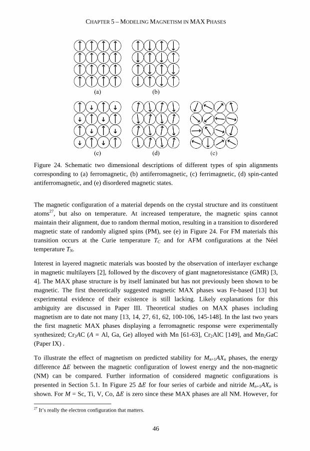
CHAPTER 5 – MODELING MAGNETISM IN MAX PHASES
46
Figure 24. Schematic two dimensional descriptions of different types of spin alignments corresponding to (a) ferromagnetic, (b) antiferromagnetic, (c) ferrimagnetic, (d) spin-canted antiferromagnetic, and (e) disordered magnetic states.
The magnetic configuration of a material depends on the crystal structure and its constituent atoms27, but also on temperature. At increased temperature, the magnetic spins cannot maintain their alignment, due to random thermal motion, resulting in a transition to disordered magnetic state of randomly aligned spins (PM), see (e) in Figure 24. For FM materials this transition occurs at the Curie temperature TC and for AFM configurations at the Néel temperature TN.
Interest in layered magnetic materials was boosted by the observation of interlayer exchange in magnetic multilayers [2], followed by the discovery of giant magnetoresistance (GMR) [3, 4]. The MAX phase structure is by itself laminated but has not previously been shown to be magnetic. The first theoretically suggested magnetic MAX phases was Fe-based [13] but experimental evidence of their existence is still lacking. Likely explanations for this ambiguity are discussed in Paper III. Theoretical studies on MAX phases including magnetism are to date not many [13, 14, 27, 61, 62, 100-106, 145-148]. In the last two years the first magnetic MAX phases displaying a ferromagnetic response were experimentally synthesized; Cr2AC (A = Al, Ga, Ge) alloyed with Mn [61-63], Cr2AlC [149], and Mn2GaC (Paper IX) .
To illustrate the effect of magnetism on predicted stability for Mn+1AXn phases, the energy
difference Δ between the magnetic configuration of lowest energy and the non-magnetic (NM) can be compared. Further information of considered magnetic configurations is
presented in Section 5.1. In Figure 25 Δ for four series of carbide and nitride Mn+1AXn is
shown. For M = Sc, Ti, V, Co, Δ is zero since these MAX phases are all NM. However, for
27 It’s really the electron configuration that matters.
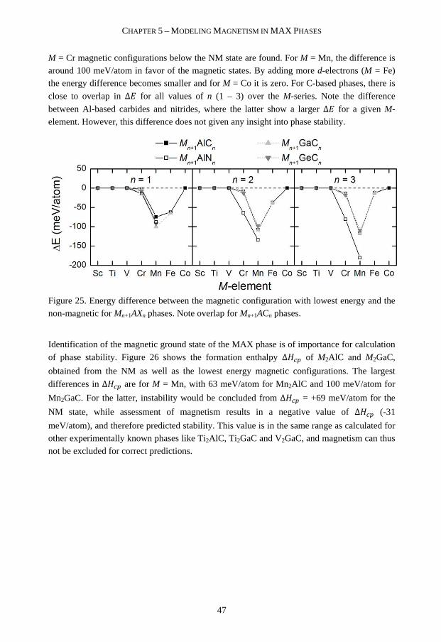
CHAPTER 5 – MODELING MAGNETISM IN MAX PHASES
47
M = Cr magnetic configurations below the NM state are found. For M = Mn, the difference is around 100 meV/atom in favor of the magnetic states. By adding more d-electrons (M = Fe) the energy difference becomes smaller and for M = Co it is zero. For C-based phases, there is
close to overlap in Δ for all values of n (1 – 3) over the M-series. Note the difference
between Al-based carbides and nitrides, where the latter show a larger Δ for a given M-element. However, this difference does not given any insight into phase stability.
Figure 25. Energy difference between the magnetic configuration with lowest energy and the non-magnetic for Mn+1AXn phases. Note overlap for Mn+1ACn phases.
Identification of the magnetic ground state of the MAX phase is of importance for calculation
of phase stability. Figure 26 shows the formation enthalpy ∆NOP of M2AlC and M2GaC,
obtained from the NM as well as the lowest energy magnetic configurations. The largest
differences in ∆NOP are for M = Mn, with 63 meV/atom for Mn2AlC and 100 meV/atom for
Mn2GaC. For the latter, instability would be concluded from ∆NOP = +69 meV/atom for the
NM state, while assessment of magnetism results in a negative value of ∆NOP (-31
meV/atom), and therefore predicted stability. This value is in the same range as calculated for other experimentally known phases like Ti2AlC, Ti2GaC and V2GaC, and magnetism can thus not be excluded for correct predictions.

CHAPTER 5 – MODELING MAGNETISM IN MAX PHASES
48
Figure 26. Calculated formation enthalpy ∆NOP for non-magnetic (open symbols) and
magnetic (filled symbols) M2AC phases where M = Ti, V, Cr, Mn, and A = Al (■ and □), Ga (● and ○)
5.1 Spin configurations of M2AX phases
Figure 25 and Figure 26 showed the importance of including magnetism in any theoretical evaluation, however, no information was given about the magnetic states considered and what spin configuration represented the low energy state. Previous studies aiming for identification of the magnetic ground state of MAX phases include at most NM, FM, and one AFM state, where the definition of the AFM state is usually excluded [13, 101, 103-106, 146, 150, 151]. This section covers theoretical treatment of magnetic spin configuration for M2AX phases, starting with collinear description (spins are (anti)parallel), followed by a few examples of possible noncollinear configurations, all exemplified by the recently theoretically predicted and experimentally verified Mn2GaC.
5.1.1 Collinear configurations
For an AFM state the set of possible collinear spin configurations are many, although, in practice, limited to configurations that maximize the number of anti-parallel moments over a few nearest neighbor shells. However, due to the symmetry of the M2AX phases there are several configurations which can fulfill this criterion. Illustrated in Figure 27 is the FM configuration (a), and five different collinear AFM configuration, (b) to (f).
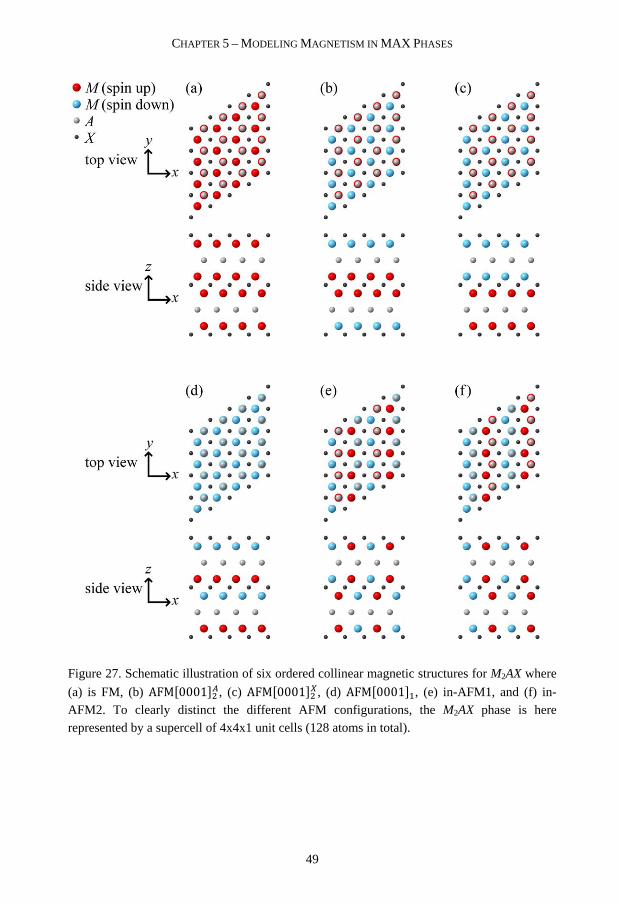
CHAPTER 5 – MODELING MAGNETISM IN MAX PHASES
49
Figure 27. Schematic illustration of six ordered collinear magnetic structures for M2AX where
(a) is FM, (b) AFM�0001�&I, (c) AFM�0001�&4, (d) AFM�0001��, (e) in-AFM1, and (f) in-AFM2. To clearly distinct the different AFM configurations, the M2AX phase is here represented by a supercell of 4x4x1 unit cells (128 atoms in total).

CHAPTER 5 – MODELING MAGNETISM IN MAX PHASES
50
The notation for these were introduced in Paper V and the corresponding interpretation for (b) to (f) are
• AFM�0001�&I, double layered AFM ordering with spins changing sign upon crossing an A atom along [0001] direction.
• AFM�0001�&4, double layered AFM ordering with spins changing sign upon crossing an X atom along [0001] direction.
• AFM�0001��, single layered AFM ordering with spins changing sign for every [0001]-layer of M atoms.
• in-AFM1 in-plane AFM.
• in-AFM2 in-plane AFM.
These can be differentiated from one another using spin correlation functions Φ� to describe the applied spins in different coordination shells α of the M atoms. The spin correlation functions, defined as the average relative orientations of the magnetic moments in the α:th coordination shell of the M atoms, is given by
Φ� = 1� 7 �9 ⋅ ��
9,�∈�, (16)
where N is the number of terms in the sum, and ei and ej are unit vectors in the direction of the local magnetic moment on site i and j. In our collinear case the spins are parallel and/or antiparallel to each other with unit vectors ei and ej of either +1 for spin up or -1 for spin
down. Three characteristic, but not limited to, values of Φ� are described as follows;
• Φ� = 1, all atoms in shell α have the same spin direction as the center atom (ei = ej).
• Φ� = -1, antiparallel configuration with opposite spin direction of all neighboring spins in shell α.
• Φ� = 0, there are in average equal amount of parallel and anti-parallel spin pairs in coordination shell α which is the case for an ideally random distribution of spins.
To distinct the six collinear magnetic configurations in Figure 27 the first four coordination shells for the M atoms are needed, illustrated by unit vectors in Figure 28. Corresponding
values Φ� for each shell α is shown in Table 14. Note that for modeling AFM within an M-plane (in-AFM1 and in-AFM2) the original unit cell of M2AX (1 × 1 × 1 with 8 atoms) is insufficient and needs to be expanded to 2 × 1 × 1 unit cells (16 atoms).

CHAPTER 5 – MODELING MAGNETISM IN MAX PHASES
51
Figure 28. Schematic illustration of unit vectors representing the first four coordination shells of M in M2AX.
Table 14. Spin correlation function Φ� for the first four coordination shells of M in M2AX. The term nα is the number of atoms in shell α, generally denoted by N in Eq. (16). Also note the unit cell needed for modeling corresponding magnetic configuration.
Magnetic configuration
Spin correlation functions Φ� Magnetic
unit cell size Φ�
(�� = 3)
Φ&
(�� = 6)
Φ�
(�� = 3)
Φ�
(�� = 1)
FM 1 1 1 1 1 × 1 × 1
AFM�0001�&I 1 1 1 -1 1 × 1 × 1
AFM�0001�&4 -1 1 -1 1 1 × 1 × 1
AFM�0001�� -1 1 -1 -1 1 × 1 × 1
in-AFM1 -1/3 -1/3 1 1 2 × 1 × 1
in-AFM2 1/3 -1/3 -1 1 2 × 1 × 1
An extension of the double-layered AFM’s, AFM�0001�&I and AFM�0001�&4, would be to increase the number of consecutive M-layers with equal spin direction before changing sign. Quadruple-, sextuple-, and octuple-layered AFM configurations are illustrated in Figure 29,
with a notation that follows the same principles as the double-layered AFM’s (AFM�0001��I
and AFM�0001��4) with z = 4, 6, 8 depending on the number of consecutive M-layers with equal spin direction. The magnetic unit cell needed for modeling the extended multi-layered AFM ordered collinear magnetic structures for M2AX are 1 × 1 × 2 unit cells (z = 4), 1 × 1 ×
3 unit cells (z = 6), and 1 × 1 × 4 unit cells (z = 8). For � → ∞ the magnetic configuration becomes FM.
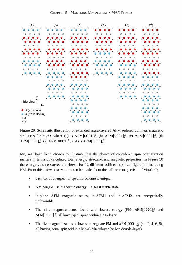
CHAPTER 5 – MODELING MAGNETISM IN MAX PHASES
52
Figure 29. Schematic illustration of extended multi-layered AFM ordered collinear magnetic
structures for M2AX where (a) is AFM�0001��I, (b) AFM�0001��I, (c) AFM�0001��I, (d)
AFM�0001��4, (e) AFM�0001��4, and (f) AFM�0001��4.
Mn2GaC have been chosen to illustrate that the choice of considered spin configuration matters in terms of calculated total energy, structure, and magnetic properties. In Figure 30 the energy-volume curves are shown for 12 different collinear spin configuration including NM. From this a few observations can be made about the collinear magnetism of Mn2GaC;
• each set of energies for specific volume is unique.
• NM Mn2GaC is highest in energy, i.e. least stable state.
• in-plane AFM magnetic states, in-AFM1 and in-AFM2, are energetically unfavorable.
• The nine magnetic states found with lowest energy (FM, AFM�0001��I and
AFM�0001��4) all have equal spins within a Mn-layer.
• The five magnetic states of lowest energy are FM and AFM�0001��I (z = 2, 4, 6, 8), all having equal spin within a Mn-C-Mn trilayer (or Mn double-layer).
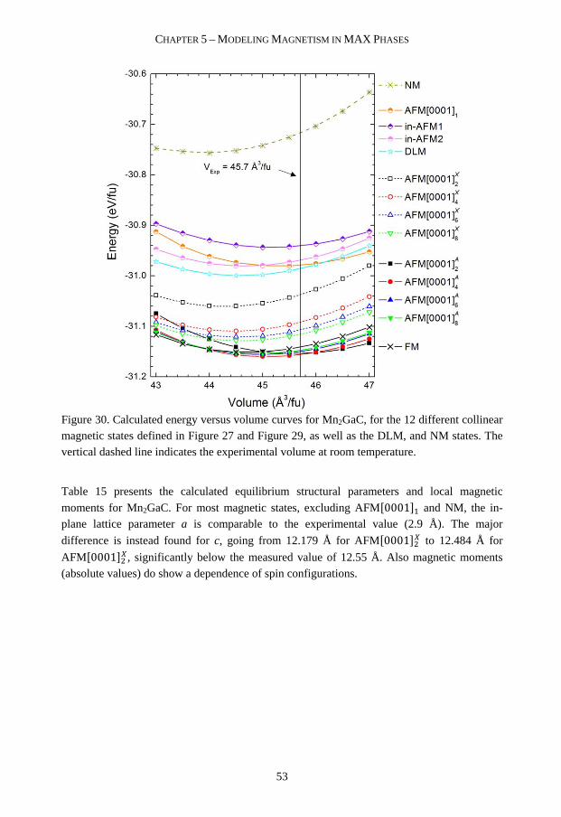
CHAPTER 5 – MODELING MAGNETISM IN MAX PHASES
53
Figure 30. Calculated energy versus volume curves for Mn2GaC, for the 12 different collinear magnetic states defined in Figure 27 and Figure 29, as well as the DLM, and NM states. The vertical dashed line indicates the experimental volume at room temperature.
Table 15 presents the calculated equilibrium structural parameters and local magnetic
moments for Mn2GaC. For most magnetic states, excluding AFM�0001�� and NM, the in-plane lattice parameter a is comparable to the experimental value (2.9 Å). The major
difference is instead found for c, going from 12.179 Å for AFM�0001�&4 to 12.484 Å for
AFM�0001�&4, significantly below the measured value of 12.55 Å. Also magnetic moments (absolute values) do show a dependence of spin configurations.

CHAPTER 5 – MODELING MAGNETISM IN MAX PHASES
54
Table 15. Calculated equilibrium volume V0 with corresponding lattice parameters a and c, and absolute magnetic moment per Mn for considered spin configurations of Mn2GaC using GGA. Experimental structural results are included for comparison.
Magnetic state
Structural parameters Local moments for Mn
atoms (��)
V0 (Å3/fu) a (Å) c (Å) GGA
NM 43.90 2.892 12.211 -
FM 44.72 2.899 12.290 1.95
AFM�0001�&I 45.57 2.903 12.484 2.26
AFM�0001�&4 44.29 2.898 12.179 1.59
AFM�0001�� 45.31 2.925 12.227 1.83
in-AFM1 45.15 2.916 12.265 1.95
in-AFM2 44.67 2.892 12.345 1.99
AFM�0001��I 45.07 2.898 12.392 1.99, 2.17
AFM�0001��I 44.96 2.900 12.344 1.92, 2.01, 2.17
AFM�0001��I 44.89 2.902 12.314 1.94, 1.97, 2.00, 2.16
AFM�0001��4 44.46 2.900 12.207 1.52, 1.95
AFM�0001��4 44.55 2.899 12.243 1.54, 1.91, 1.97
AFM�0001��4 44.60 2.899 12.258 1.54, 1.94, 1.96, 1.97
DLM 44.67 2.887 12.375 0.57 - 2.27
Expt.* 45.70 2.9 12.55
* Reference [27].
5.1.2 Noncollinear configurations
The collinear description with (anti)parallel spins is often enough for describing magnetism in a material. However, some systems require an additional degree of freedom. Within a noncollinear configuration the relative directions of the spins can span over all spatial directions. One example is the complex cubic ground-state crystal structure of Mn, known as α-Mn, which is paramagnetic at ambient conditions. At the Néel temperature of 95 K, there is a transition to a complex noncollinear antiferromagnetic phases [152, 153].
Another example is Cr and Mn monolayers on a hexagonal lattice which are prototypical examples of frustrated spin systems in two dimensions [154, 155]. The best collinear description for a nearest neighbor AFM configuration in such lattice is the row-wise AFM illustrated in Figure 31(a). For MAX phases this corresponds to in-AFM1 and in-AFM2. For a hexagonal lattice the classical nearest neighbor Heisenberg model predicts a noncollinear ground state consisting of a three atom unit cell with magnetic moments aligned ±120°, also known as the coplanar noncollinear Néel (120°) structure, see Figure 31(b).

CHAPTER 5 – MODELING MAGNETISM IN MAX PHASES
55
Figure 31. (a) The row-wise AFM structure and (b) the noncollinear Néel (120°) structure with corresponding two- and three-atom unit cell indicated. In (a) two different unit cells are illustrated; 2×1×1 hexagonal which is the base for in-AFM1 and in-AFM2 and a rectangular base which would be represented by an orthorhombic unit cell for e.g. MAX phases
Introducing noncollinearity for MAX phases could thus lead to a large number of possible magnetic configurations. As a first step, in-plane AFM of Mn2GaC have been modelled using the Néel structure within each Mn-layer. To include the effect from interaction between Mn atoms in layer i and i+1, different relative angles of the Néel structures between the individual layers have been considered. In Figure 32 the energy for five different layering of noncollinear Néel spin structure is shown for Mn2GaC, and three distinct energy-volume curves are evident. Common for the low energy Néel structures 1111 and 1771 is the equivalent relative orientation of the three spins for three Mn atoms above and below the Ga-layer. For the high energy Néel structures 1717 and 1177 the configuration above and below a
Ga layer is antiparallel. In comparison to the collinear AFM states (AFM�0001��, in-AFM1, in-AFM2) the Néel states are less energetically favored.
Figure 32. Calculated energy versus volume curves for five different layering of noncollinear Néel 120° spin structure (solid lines) and three collinear AFM states (dashed lines).

CHAPTER 5 – MODELING MAGNETISM IN MAX PHASES
56
Another approach to model noncollinear configurations is to explore the change in energy, structure, and magnetic properties in between two collinear configurations. One such example is canted spins, illustrated in Figure 33, where the anti-parallel spins in (a), corresponding to
the collinear AFM�0001��I, are canted by θc degrees in +z direction (b) giving rise to a small net moment. Further canting of the spins eventually results in parallel spins (c), corresponding to FM.
Figure 33. Schematic illustration of spins canted by an angle θc where (a) is AFM�0001��I
(θc = 180°), (b) an intermediate state (θc ≈ 155°), and (c) FM (θc = 0°). Note that the spins can as well be canted within the M-planes, i.e. rotated around the z-axis, but for illustrative reasons the rotation is around the y-axis. Such choice is only of importance when including spin-orbit coupling.
In Figure 34(a) the total energy as a function of canting angle θc is shown for a relaxed and
two fixed lattices of Mn2GaC. As θc is increased, the magnetic state changes continuously
from FM at θc = 0° to AFM�0001��I at θc = 180°, for both fixed and relaxed lattices. For
angles close to 0° and 180° the corresponding fixed lattice represents the relaxed lattice well. In panel (b) of Figure 34 the local magnetic moment (absolute values) show a small but
gradual increase as θc is increased. For half of the Mn atoms this is more pronounced, a structural-magnetic effect which will be further discussed below. Also shown is the net
magnetization which gradually decreases as θc increases, from 1.83 �� per Mn atom for the
FM state to zero at θc = 180°. Close to θc = 180° this decrease is most pronounced, although
accompanied by only minor changes in energy; between 150° and 180°, the energy changes with less than 1 meV/fu.
For the relaxed lattice it is possible to see how the structural parameters are affected upon spin
canting. In Figure 35(a) there is an almost unaffected basal plane lattice parameter a for all θc, as opposed to the lattice parameter c which increases continuously from 12.29 Å (FM) to 12.39 Å (AFM). This increase can be related to the change in the Mn interlayer distance of Mn-Ga-Mn, but only if the two Mn-layers have anti-parallel spin. For corresponding parallel
spins the interlayer distance is almost unaffected by θc.
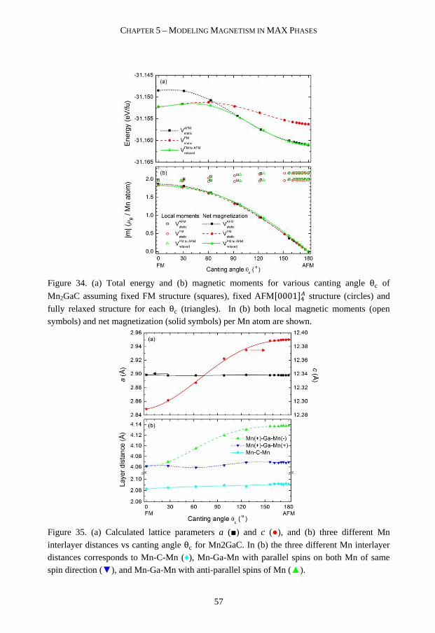
CHAPTER 5 – MODELING MAGNETISM IN MAX PHASES
57
Figure 34. (a) Total energy and (b) magnetic moments for various canting angle θc of
Mn2GaC assuming fixed FM structure (squares), fixed AFM�0001��I structure (circles) and
fully relaxed structure for each θc (triangles). In (b) both local magnetic moments (open symbols) and net magnetization (solid symbols) per Mn atom are shown.
Figure 35. (a) Calculated lattice parameters a (■) and c (●), and (b) three different Mn
interlayer distances vs canting angle θc for Mn2GaC. In (b) the three different Mn interlayer distances corresponds to Mn-C-Mn (♦), Mn-Ga-Mn with parallel spins on both Mn of same spin direction (▼), and Mn-Ga-Mn with anti-parallel spins of Mn (▲).
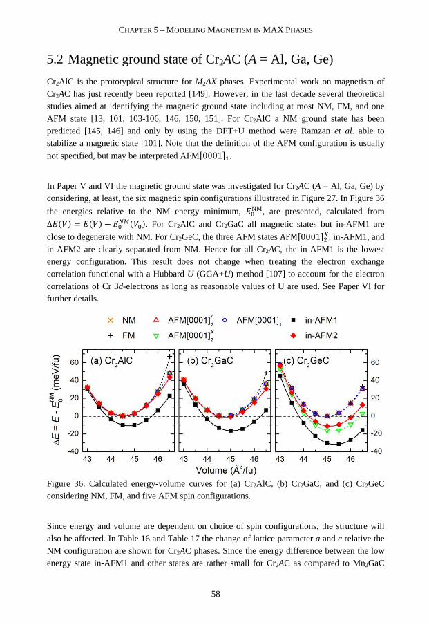
CHAPTER 5 – MODELING MAGNETISM IN MAX PHASES
58
5.2 Magnetic ground state of Cr2AC (A = Al, Ga, Ge)
Cr2AlC is the prototypical structure for M2AX phases. Experimental work on magnetism of Cr2AC has just recently been reported [149]. However, in the last decade several theoretical studies aimed at identifying the magnetic ground state including at most NM, FM, and one AFM state [13, 101, 103-106, 146, 150, 151]. For Cr2AlC a NM ground state has been predicted [145, 146] and only by using the DFT+U method were Ramzan et al. able to stabilize a magnetic state [101]. Note that the definition of the AFM configuration is usually
not specified, but may be interpreted AFM�0001��.
In Paper V and VI the magnetic ground state was investigated for Cr2AC (A = Al, Ga, Ge) by considering, at least, the six magnetic spin configurations illustrated in Figure 27. In Figure 36
the energies relative to the NM energy minimum, !��, are presented, calculated from
Δ��� = ��� − !8W��!�. For Cr2AlC and Cr2GaC all magnetic states but in-AFM1 are
close to degenerate with NM. For Cr2GeC, the three AFM states AFM�0001�&4, in-AFM1, and in-AFM2 are clearly separated from NM. Hence for all Cr2AC, the in-AFM1 is the lowest energy configuration. This result does not change when treating the electron exchange correlation functional with a Hubbard U (GGA+U) method [107] to account for the electron correlations of Cr 3d-electrons as long as reasonable values of U are used. See Paper VI for further details.
Figure 36. Calculated energy-volume curves for (a) Cr2AlC, (b) Cr2GaC, and (c) Cr2GeC considering NM, FM, and five AFM spin configurations.
Since energy and volume are dependent on choice of spin configurations, the structure will also be affected. In Table 16 and Table 17 the change of lattice parameter a and c relative the NM configuration are shown for Cr2AC phases. Since the energy difference between the low energy state in-AFM1 and other states are rather small for Cr2AC as compared to Mn2GaC

CHAPTER 5 – MODELING MAGNETISM IN MAX PHASES
59
and the hypothetical Mn2AlC, see e.g. Figure 25, the latter two has also been included. Cr-based phases are moderately affected by choice of magnetic configuration with largest changes for in-AFM1. For Mn2AlC the effect of including spin correlation is most
pronounced in-plane with ∆g ≈ 1.5 % whereas Mn2GaC have a spread of from 0 to +1.2%. The relative change in c is more wide spread, -1.0% to +2.2% indicating that magnetic interactions out-of-plane, e.g. across the X-layer, play an important role in finding the magnetic ground-state.
Table 16. Relative change in lattice parameter a (in %) for different magnetic configurations relative NM for five M2AC phases. Values for NM are given in bottom row.
Magnetic configuration
∆a relative NM (%)
Cr2AlC Cr2GaC Cr2GeC Mn2AlC Mn2GaC
FM 0.1 0.0 0.0 1.4 0.3
AFM�0001�&I 0.1 0.0 0.0 1.5 0.4
AFM�0001�&4 0.1 0.0 0.0 1.5 0.2
AFM�0001�� 0.0 0.0 0.0 1.9 1.2
in-AFM1 0.2 0.4 0.5 1.5 0.8
in-AFM2 0.1 0.1 0.3 1.3 0.0
AFM�0001��I 0.0 0.0 0.1 1.6 0.2
AFM�0001��4 0.0 0.0 0.1 1.5 0.3
aNM (Å) 2.844 2.871 2.937 2.824 2.892
Table 17. Relative change in lattice parameter c (in %) for different magnetic configurations relative NM for five M2AC phases. Values for are NM given in bottom row.
Magnetic configuration
∆c relative NM (%)
Cr2AlC Cr2GaC Cr2GeC Mn2AlC Mn2GaC
FM -0.1 0.0 -0.1 -0.2 0.6
AFM�0001�&I -0.1 0.0 0.0 1.9 2.2
AFM�0001�&4 -0.1 0.0 0.1 -1.0 -0.2
AFM�0001�� 0.0 0.0 0.0 -0.2 0.2
in-AFM1 0.2 0.1 -0.1 0.1 0.4
in-AFM2 -0.1 0.0 -0.2 0.0 1.1
AFM�0001��I 0.0 0.0 0.0 0.7 1.6
AFM�0001��4 0.0 0.0 0.1 -0.7 0.0
cNM (Å) 12.707 12.531 12.036 12.466 12.211
Choice of magnetic configuration also affect the calculated materials properties, here exemplified by the bulk modulus B0. In the M2AlC series (M = Ti, V, Cr) there has been an ongoing discussion concerning the deviation between first principles calculations and
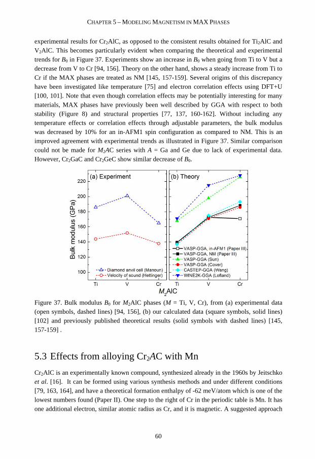
CHAPTER 5 – MODELING MAGNETISM IN MAX PHASES
60
experimental results for Cr2AlC, as opposed to the consistent results obtained for Ti2AlC and V2AlC. This becomes particularly evident when comparing the theoretical and experimental trends for B0 in Figure 37. Experiments show an increase in B0 when going from Ti to V but a decrease from V to Cr [94, 156]. Theory on the other hand, shows a steady increase from Ti to Cr if the MAX phases are treated as NM [145, 157-159]. Several origins of this discrepancy have been investigated like temperature [75] and electron correlation effects using DFT+U [100, 101]. Note that even though correlation effects may be potentially interesting for many materials, MAX phases have previously been well described by GGA with respect to both stability (Figure 8) and structural properties [77, 137, 160-162]. Without including any temperature effects or correlation effects through adjustable parameters, the bulk modulus was decreased by 10% for an in-AFM1 spin configuration as compared to NM. This is an improved agreement with experimental trends as illustrated in Figure 37. Similar comparison could not be made for M2AC series with A = Ga and Ge due to lack of experimental data. However, Cr2GaC and Cr2GeC show similar decrease of B0.
Figure 37. Bulk modulus B0 for M2AlC phases (M = Ti, V, Cr), from (a) experimental data (open symbols, dashed lines) [94, 156], (b) our calculated data (square symbols, solid lines) [102] and previously published theoretical results (solid symbols with dashed lines) [145, 157-159] .
5.3 Effects from alloying Cr2AC with Mn
Cr2AlC is an experimentally known compound, synthesized already in the 1960s by Jeitschko et al. [16]. It can be formed using various synthesis methods and under different conditions [79, 163, 164], and have a theoretical formation enthalpy of -62 meV/atom which is one of the lowest numbers found (Paper II). One step to the right of Cr in the periodic table is Mn. It has one additional electron, similar atomic radius as Cr, and it is magnetic. A suggested approach
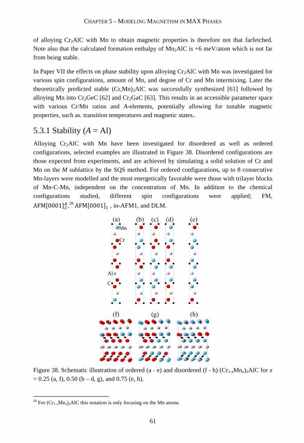
CHAPTER 5 – MODELING MAGNETISM IN MAX PHASES
61
of alloying Cr2AlC with Mn to obtain magnetic properties is therefore not that farfetched. Note also that the calculated formation enthalpy of Mn2AlC is +6 meV/atom which is not far from being stable.
In Paper VII the effects on phase stability upon alloying Cr2AlC with Mn was investigated for various spin configurations, amount of Mn, and degree of Cr and Mn intermixing. Later the theoretically predicted stable (Cr,Mn)2AlC was successfully synthesized [61] followed by alloying Mn into Cr2GeC [62] and Cr2GaC [63]. This results in an accessible parameter space with various Cr/Mn ratios and A-elements, potentially allowing for tunable magnetic properties, such as. transition temperatures and magnetic states..
5.3.1 Stability (A = Al)
Alloying Cr2AlC with Mn have been investigated for disordered as well as ordered configurations, selected examples are illustrated in Figure 38. Disordered configurations are those expected from experiments, and are achieved by simulating a solid solution of Cr and Mn on the M sublattice by the SQS method. For ordered configurations, up to 8 consecutive Mn-layers were modelled and the most energetically favorable were those with trilayer blocks of Mn-C-Mn, independent on the concentration of Mn. In addition to the chemical configurations studied, different spin configurations were applied; FM,
AFM�0001�&{,28 AFM�0001�� , in-AFM1, and DLM.
Figure 38. Schematic illustration of ordered (a - e) and disordered (f - h) (Cr1-xMnx)2AlC for x = 0.25 (a, f), 0.50 (b – d, g), and 0.75 (e, h).
28 For (Cr1-xMnx)2AlC this notation is only focusing on the Mn atoms.

CHAPTER 5 – MODELING MAGNETISM IN MAX PHASES
62
In Table 18 the identified set of most competing phases, including and excluding Cr2AlC, are given for (Cr1-xMnx)2AlC. Due to the stability of Cr2AlC, the set of most competing phases which includes Cr2AlC will be lower in energy, and therefore also used in the upcoming results.
Table 18. Identified set of most competing phases (cp) for (Cr1-xMnx)2AlC including and excluding Cr2AlC as cp.
Identified set of most competing phases
x all cp all cp, excluding MAX phases
0.00 Cr2AlC Cr2Al, C3C2, Al4C3
0.25 Cr2AlC, MnAl, C, Mn3AlC Cr3C2, MnAl, Mn4Al 11
0.50 Cr2AlC, MnAl, C, Mn3AlC MnAl, C, Cr3C2
0.75 Cr2AlC, MnAl, C, Mn3AlC MnAl, C, Mn3AlC, C3C2
1.00 MnAl, C, Mn3AlC MnAl, C, Mn3AlC
In Figure 39 the formation enthalpy ∆NOP for ordered and disordered configurations of (Cr1-
xMnx)2AlC is shown. Ordered systems have negative values of ∆NOP with a minimum of -10
meV/ atom for a Mn-C-Mn configuration at x = 0.50, corresponding to (b) in Figure 38. This
ordered FM state is also found to be degenerate with AFM�0001�&I. In comparison, ordered configurations (c) and (d) are higher in energy by +7 meV/atom and +25 meV/atom, respectively. In common for (b) and (c) are the Mn-C-Mn trilayer which seems energetically favorable as compared to other chemical configurations.
Disordered configurations, on the other hand, show positive values of ∆NOP, with a maximum
of +12 meV/atom for the FM magnetic states at x = 0.50. Note that FM is favorable as compared to AFM states. However, at elevated temperatures, the configurational entropy due
to the solid solution of Cr and Mn will lower the displayed curve, e.g., at 600 K ∆NOP is
estimated to -6 meV/atom.

CHAPTER 5 – MODELING MAGNETISM IN MAX PHASES
63
Figure 39. Calculated formation enthalpy ∆NOP for configurationally ordered (open symbols)
and disordered (filled symbols) FM and various AFM states of (Cr1-xMx)2AlC. Letters within parenthesis corresponds to schematics in Figure 38.
Magnetic moments for ordered (Figure 40) and disordered (Figure 41) configurations show
that the major contribution to magnetism comes from Mn atoms (around 2 ��). Cr moments instead show an evident dependence on surrounding atoms. Ordered systems, with layers of Cr (and Mn), have Cr moments of about 1/8th relative to those of Mn. Note that for the low energy configurations, with blocks of Mn-C-Mn and Cr-C-Cr trilayers (a - d in Figure 40), Cr atoms adjacent to a Mn-layer always have the same orientation as the Mn moment. When there is a mixture of Cr and Mn within a M-layer, i.e. disordered solutions, an increase of the
(average) Cr moments is clear, 0.5 to 0.7 �� depending on magnetic state and amount of Mn (x). From this information the exchange coupling between Cr and Mn atoms seem to be dependent on the underlying chemical ordering.
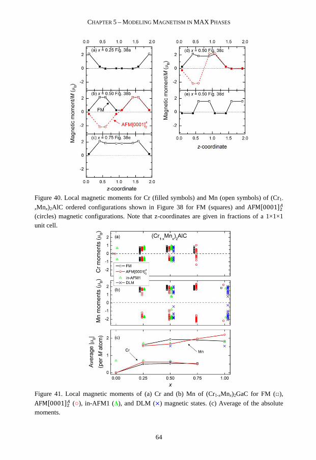
CHAPTER 5 – MODELING MAGNETISM IN MAX PHASES
64
Figure 40. Local magnetic moments for Cr (filled symbols) and Mn (open symbols) of (Cr1-
xMnx)2AlC ordered configurations shown in Figure 38 for FM (squares) and AFM�0001�&I (circles) magnetic configurations. Note that z-coordinates are given in fractions of a 1×1×1 unit cell.
Figure 41. Local magnetic moments of (a) Cr and (b) Mn of (Cr1-xMnx)2GaC for FM (□),
AFM�0001�&I (○), in-AFM1 (∆), and DLM (×) magnetic states. (c) Average of the absolute moments.

CHAPTER 5 – MODELING MAGNETISM IN MAX PHASES
65
5.3.2 Intermixing – from order to disorder (A = Al)
(Cr0.50Mn0.50)2AlC in Figure 39 have degenerate ground states for ordered Mn-C-Mn configurations, while the FM state is energetically favorable for the solid solution. To evaluate the states between these configurations, Figure 42 show a detailed evaluation of the energies when going from chemical order to disorder, by gradually increasing the intermixing of Cr into the Mn-C-Mn trilayers, and conversely Mn into the Cr-C-Cr trilayers. Panel (a)
displays a gradual increase of ∆NOP with increasing disorder. Ppanel (b) show the energy for
different AFM states relative to FM configuration. For complete order the FM and
AFM�0001�&I are considered as degenerate states with an energy difference of just 0.4 meV/atom in favor of AFM. This can be compared to the result for disordered Mn and Cr moments (DLM state) at +23 meV/atom. This ground-state degeneracy is present up to a semi-degree of intermixing followed by a stabilization of the FM state at increased disorder.
For complete disorder of Cr and Mn, FM is most stable, 3 mwV/atom below AFM�0001�&I and other AFM states. Compared to DLM the difference is 10 meV/atom.
Figure 42. (a) Formation enthalpy of (Cr0.5Mn0.5)2AlC in its most stable magnetic state, and
(b) the energy of AFM�0001�&I, AFM, and DLM states relative to the FM state, as a function of the degree of M-site intermixing. The latter is defined as Cr concentration in Mn-C-Mn trilayers where 0 and 0.50 corresponds to configurations (b) and (g) in Figure 38.
5.4 Magnetic ground state of Mn2GaC
From experiments it is known that Mn2GaC is magnetic, but the details of the magnetic ground state remains to be determined [27]. Figure 30 shows that spin configurations with

CHAPTER 5 – MODELING MAGNETISM IN MAX PHASES
66
spins aligned parallel within a Mn-C-Mn trilayer, FM and AFM�0001��I, are energetically favored, with α = 4 of lowest energy as compared to other collinear spin configurations. However, as there can be magnetic states which have been overlooked, a magnetic ground-state search is justified.
5.4.1 Super-moment model
In order to perform a complete magnetic ground-state search, large structures are needed to avoid limiting size effects. Also magnetic exchange interaction (MEI) parameters are required. However, we instead make use of the information in Figure 30 that spins aligned
parallel within a Mn-C-Mn trilayer are energetically favored, i.e. FM and AFM�0001��I (z = 2, 4, 6, 8). A coarse-grained model was proposed in Paper IX where each trilayer is seen as a super-moment. Hence, within a super-moment the magnetic interaction of Mn atoms within layers and across the C-layer is neglected. Only magnetic interactions between different trilayers are considered, and the model can thus be seen as an atomic chain. A schematic of this coarse-grained super-moment model is illustrated in Figure 43. The spin correlation
functions Φ� shown in Table 19 are obtained through use of Eq. (16) for the first four super-moment coordination shells of each of the five magnetic structures.
Figure 43. Super-moment model for the five low-energy collinear magnetic spin configurations of Mn2GaC in Figure 30. Here the magnetic chains are constructed by 30
super-moment beads. Note that the spin-correlation function Φ� for the four nearest neighbors are specified by arrows.
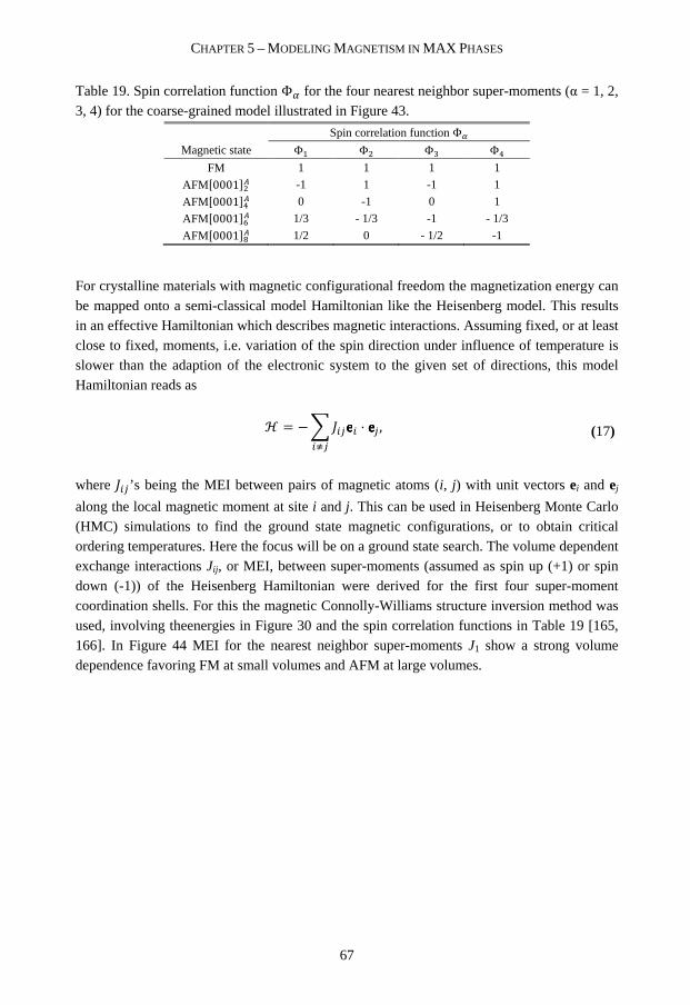
CHAPTER 5 – MODELING MAGNETISM IN MAX PHASES
67
Table 19. Spin correlation function Φ� for the four nearest neighbor super-moments (α = 1, 2, 3, 4) for the coarse-grained model illustrated in Figure 43.
Spin correlation function Φ�
Magnetic state Φ� Φ& Φ� Φ�
FM 1 1 1 1
AFM�0001�&I -1 1 -1 1
AFM�0001��I 0 -1 0 1
AFM�0001��I 1/3 - 1/3 -1 - 1/3
AFM�0001��I 1/2 0 - 1/2 -1
For crystalline materials with magnetic configurational freedom the magnetization energy can be mapped onto a semi-classical model Hamiltonian like the Heisenberg model. This results in an effective Hamiltonian which describes magnetic interactions. Assuming fixed, or at least close to fixed, moments, i.e. variation of the spin direction under influence of temperature is slower than the adaption of the electronic system to the given set of directions, this model Hamiltonian reads as
ℋ = − 7 ¡9�eeee99¢�
⋅ eeee� , (17)
where ¡9� ’s being the MEI between pairs of magnetic atoms (i, j) with unit vectors ei and ej
along the local magnetic moment at site i and j. This can be used in Heisenberg Monte Carlo (HMC) simulations to find the ground state magnetic configurations, or to obtain critical ordering temperatures. Here the focus will be on a ground state search. The volume dependent exchange interactions Jij, or MEI, between super-moments (assumed as spin up (+1) or spin down (-1)) of the Heisenberg Hamiltonian were derived for the first four super-moment coordination shells. For this the magnetic Connolly-Williams structure inversion method was used, involving theenergies in Figure 30 and the spin correlation functions in Table 19 [165, 166]. In Figure 44 MEI for the nearest neighbor super-moments J1 show a strong volume dependence favoring FM at small volumes and AFM at large volumes.
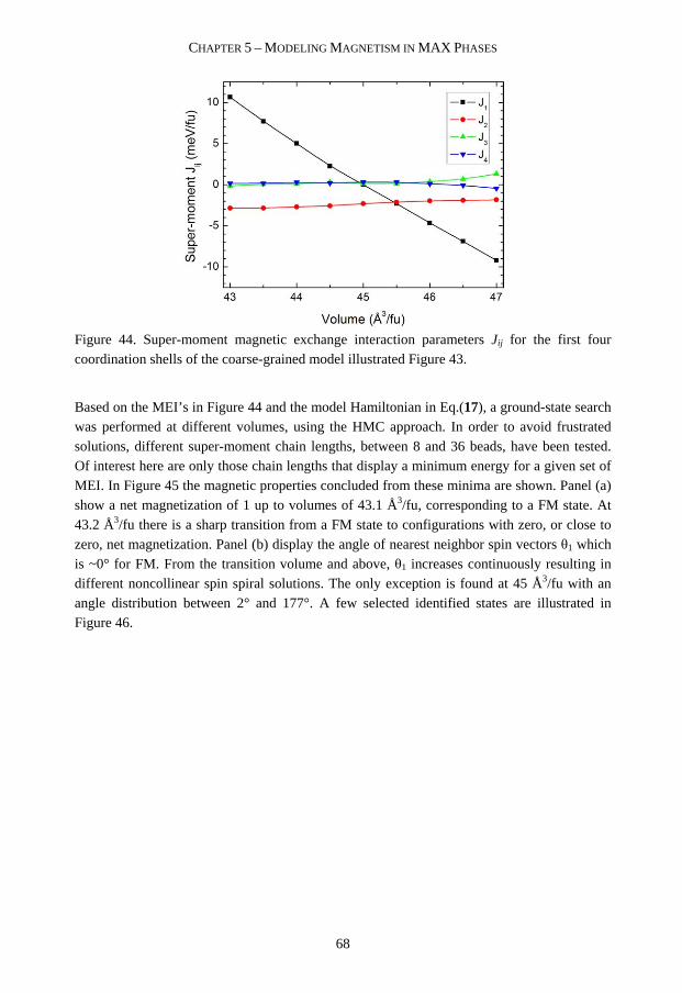
CHAPTER 5 – MODELING MAGNETISM IN MAX PHASES
68
Figure 44. Super-moment magnetic exchange interaction parameters Jij for the first four coordination shells of the coarse-grained model illustrated Figure 43.
Based on the MEI’s in Figure 44 and the model Hamiltonian in Eq.(17), a ground-state search was performed at different volumes, using the HMC approach. In order to avoid frustrated solutions, different super-moment chain lengths, between 8 and 36 beads, have been tested. Of interest here are only those chain lengths that display a minimum energy for a given set of MEI. In Figure 45 the magnetic properties concluded from these minima are shown. Panel (a) show a net magnetization of 1 up to volumes of 43.1 Å3/fu, corresponding to a FM state. At 43.2 Å3/fu there is a sharp transition from a FM state to configurations with zero, or close to zero, net magnetization. Panel (b) display the angle of nearest neighbor spin vectors θ1 which is ~0° for FM. From the transition volume and above, θ1 increases continuously resulting in different noncollinear spin spiral solutions. The only exception is found at 45 Å3/fu with an angle distribution between 2° and 177°. A few selected identified states are illustrated in Figure 46.

CHAPTER 5 – MODELING MAGNETISM IN MAX PHASES
69
Figure 45. (a) Net magnetization of low energy configurations and (b) angle between nearest neighbor superatom spins as a function of volume for HMC simulations. Data for different chain lengths of minimum energy shown as × and corresponding average by red dashed lines. Inset in (a) show a close up of the transition from FM to AFM.
Figure 46. Examples of magnetic states at different volumes as obtained from HMC simulations. Chosen volumes are (a) 43.0, (b) 43.1, (c) 43.2, (d) 43.7, (e) and (f) 45.0, and (g) 46.0 Å3/fu.
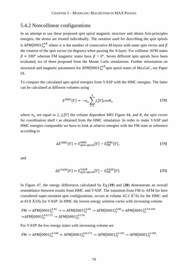
CHAPTER 5 – MODELING MAGNETISM IN MAX PHASES
70
5.4.2 Noncollinear configurations
In an attempt to use these proposed spin spiral magnetic structure and obtain first-principles energies, the atoms are treated individually. The notation used for describing the spin spirals
is AFM�0001��I,£ where ¤ is the number of consecutive M-layers with same spin vector and ¥
the rotation of the spin vector (in degrees) when passing the A-layer. For collinear AFM states
¥ = 180° whereas FM magnetic states have ¥ = 0°. Seven different spin spirals have been evaluated, six of them proposed from the Monte Carlo simulations. Further information on
structural and magnetic parameters for AFM�0001��I,£spin spiral states of Mn2GaC, see Paper
IX.
To compare the calculated spin spiral energies from VASP with the HMC energies. The latter can be calculated at different volumes using
¦�x��� = −�� 7 ¡9���i§¨©9�
9:�, (18)
where �� are equal to 2, ¡9��� the volume dependent MEI Figure 44, and ©9 the spin vector for coordination shell i as obtained from the HMC simulation. In order to make VASP and HMC energies comparable we have to look at relative energies with the FM state as reference according to
Δ¦�x��� = ª�+« ª�+z¬|¦�x ��� − �¦�x���, (19)
and
Δ®{¯°��� = ª�+« ª�+z¬|®{¯° ��� − �®{¯°���. (20)
In Figure 47, the energy differences calculated by Eq.(19) and (20) demonstrate an overall resemblance between results from HMC and VASP. The transition from FM to AFM for here considered super-moment spin configurations, occurs at volume 43.3 Å3/fu for the HMC and at 43.8 Å3/fu for VASP. In HMC the lowest energy solution varies with increasing volume
FM → AFM�0001�&I,�± → = AFM�0001�&I,�! → AFM�0001�&I,²!= AFM�0001�&I,³�,�!� =AFM�0001�&I,�,�³& → AFM�0001�&I,�&!.
For VASP the low energy states with increasing volume are
FM → AFM�0001��I,��! ≈ AFM�0001�&I,�,�³& → AFM�0001�&I,�&! → AFM�0001�&I,��!.
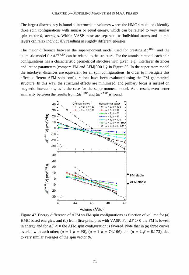
CHAPTER 5 – MODELING MAGNETISM IN MAX PHASES
71
The largest discrepancy is found at intermediate volumes where the HMC simulations identify three spin configurations with similar or equal energy, which can be related to very similar
spin vector ©9 averages. Within VASP these are separated as individual atoms and atomic layers can relax individually resulting in slightly different energies.
The major difference between the super-moment model used for creating Ħ�x and the
atomistic model for Δ®{¯° can be related to the structure. For the atomistic model each spin configurations has a characteristic geometrical structure with given, e.g., interlayer distances
and lattice parameters (compare FM and AFM�0001��I in Figure 35. In the super atom model the interlayer distances are equivalent for all spin configurations. In order to investigate this effect, different AFM spin configurations have been evaluated using the FM geometrical structure. In this way, the structural effects are minimized, and primary focus is instead on magnetic interactions, as is the case for the super-moment model. As a result, even better
similarity between the results from Δ¦�x and Δ®{¯° is found.
Figure 47. Energy difference of AFM vs FM spin configurations as function of volume for (a)
HMC based energies, and (b) from first-principles with VASP. For ∆ > 0 the FM is lowest
in energy and for ∆ < 0 the AFM spin configuration is favored. Note that in (a) three curves
overlap with each other; (¤ = 2, ¥ = 90), (¤ = 2, ¥ = 74,106), and (¤ = 2, ¥ = 8,172), due
to very similar averages of the spin vector ©9.

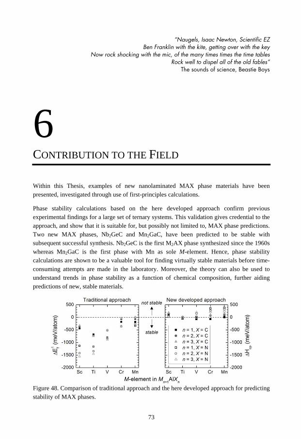
73
“Naugels, Isaac Newton, Scientific EZ Ben Franklin with the kite, getting over with the key
Now rock shocking with the mic, of the many times times the time tables Rock well to dispel all of the old fables”
The sounds of science, Beastie Boys
6
CONTRIBUTION TO THE FIELD
Within this Thesis, examples of new nanolaminated MAX phase materials have been presented, investigated through use of first-principles calculations.
Phase stability calculations based on the here developed approach confirm previous experimental findings for a large set of ternary systems. This validation gives credential to the approach, and show that it is suitable for, but possibly not limited to, MAX phase predictions. Two new MAX phases, Nb2GeC and Mn2GaC, have been predicted to be stable with subsequent successful synthesis. Nb2GeC is the first M2AX phase synthesized since the 1960s whereas Mn2GaC is the first phase with Mn as sole M-element. Hence, phase stability calculations are shown to be a valuable tool for finding virtually stable materials before time-consuming attempts are made in the laboratory. Moreover, the theory can also be used to understand trends in phase stability as a function of chemical composition, further aiding predictions of new, stable materials.
Figure 48. Comparison of traditional approach and the here developed approach for predicting stability of MAX phases.
CHAPTER 6 – CONTRIBUTION TO THE FIELD
74
The theoretical phase stability approach has also been used to investigate MAX phase alloys. Incorporation of oxygen in synthesized MAX phases indicates different location of oxygen depending on choice of M-element. From both phase stability calculations and electronic structure analysis it has been suggested to be related to the number of M d-electrons. For Ti2AlC, the calculations show that oxygen act as a stabilizer, which can explain the large amount (12.5 at%) of oxygen found in synthesized samples.
In the last two years, experimental confirmation of magnetic MAX phases has been presented. Furthermore, it has been theoretically demonstrated that there are many possible magnetic spin configurations for the MAX phase structure. Diverging approaches and approximations have shown that the choice of spin configuration is of importance for phase stability predictions, identification of magnetic ground-state, and for evaluation of selected properties. The well-known Cr2AC (Al = Al, Ga, Ge) phases have here been predicted to have an in-plane AFM as a low energy state, and the effect of electron-correlation approximation on this result is believed to be of minor importance, as compared to the choice of spin configuration. Alloying Cr2AC with Mn to obtain magnetic properties is also predicted to give both FM and AFM configurations, depending on both chemical composition and chemical order/disorder. Magnetic MAX phases in all these systems, Cr2AC (Al = Al, Ga, Ge), have been experimentally synthesized, and a magnetic response verified. Advancing beyond alloying, the pure Mn2GaC has been predicted to have a large number of exotic low-energy magnetic states, with a spin-canted multilayered AFM suggested as the magnetic ground-state at low temperatures. The indicated complex magnetism remains to be experimentally verified.
75
“From up and down, and still somehow It’s cloud illusions I recall
I really don’t know clouds at all” Both sides now, Joni Mitchell
7
BIBLIOGRAPHY
[1] W. Lowrie, Fundamentals of Geophysics (Cambridge University Press, New York, 2007).
[2] P. Grünberg, R. Schreiber, Y. Pang, M. B. Brodsky, and H. Sowers, Phys. Rev. Lett. 57, 2442 (1986).
[3] M. N. Baibich, J. M. Broto, A. Fert, F. N. Van Dau, F. Petroff, P. Etienne, G. Creuzet, A. Friederich, and J. Chazelas, Phys. Rev. Lett. 61, 2472 (1988).
[4] G. Binasch, P. Grünberg, F. Saurenbach, and W. Zinn, Phys. Rev. B 39, 4828 (1989). [5] D. T. Pierce, J. Unguris, R. J. Celotta, and M. D. Stiles, J. Magn. Magn. Mater. 200, 290
(1999). [6] A. Schreyer, J. F. Ankner, T. Zeidler, H. Zabel, M. Schäfer, J. A. Wolf, P. Grünberg,
and C. F. Majkrzak, Phys. Rev. B 52, 16066 (1995). [7] C. A. F. Vaz, J. A. C. Bland, and G. Lauhoff, Rep. Prog. Phys. 71, 056501 (2008). [8] D. T. Pierce, A. D. Davies, J. A. Stroscio, D. A. Tulchinsky, J. Unguris, and R. J.
Celotta, J. Magn. Magn. Mater. 222, 13 (2000). [9] D. A. Tulchinsky, J. Unguris, and R. J. Celotta, J. Magn. Magn. Mater. 212, 91 (2000). [10] M. W. Barsoum, Prog. Solid State Chem. 28, 201 (2000). [11] P. Eklund, M. Beckers, U. Jansson, H. Högberg, and L. Hultman, Thin Solid Films 518,
1851 (2010). [12] J. Rosen, M. Dahlqvist, S. I. Simak, D. R. McKenzie, and M. M. M. Bilek, Appl. Phys.
Lett. 97, 073103 (2010). [13] W. Luo and R. Ahuja, J. Phys. Cond. Matter 20, 064217 (2008). [14] M. Dahlqvist, B. Alling, I. A. Abrikosov, and J. Rosen, Phys. Rev. B 84, 220403
(2011). [15] H. Nowotny, Prog. Solid State Chem. 5, 27 (1971). [16] W. Jeitschko, H. Nowotny, and F. Benesovsky, Monatshefte für Chemie 94, 672 (1963). [17] W. Jeitschko, H. Nowotny, and F. Benesovsky, Monatsh. Chem. 94, 844 (1963).

CHAPTER 7 – BIBLIOGRAPHY
76
[18] W. Jeitschko, H. Nowotny, and F. Benesovsky, Monatshefte für Chemie 94, 1198 (1963).
[19] W. Jeitschko, H. Nowotny, and F. Benesovsky, Monatshefte für Chemie 94, 1201 (1963).
[20] W. Jeitschko, H. Nowotny, and F. Benesovsky, Monatsh. Chem. 95, 178 (1964). [21] W. Jeitschko, H. Nowotny, and F. Benesovsky, Monatshefte für Chemie 95, 431 (1964). [22] W. Jeitschko and H. Nowotny, Monatshefte für Chemie 98, 329 (1967). [23] H. Wolfsgruber, H. Nowotny, and F. Benesovsky, Monatshefte für Chemie 98, 2403
(1967). [24] M. W. Barsoum and T. El-Raghy, J. Am. Ceram. Soc. 79, 1953 (1996). [25] M. W. Barsoum, L. Farber, I. Levin, A. Procopio, T. El-Raghy, and A. Berner, J. Am.
Ceram. Soc. 82, 2545 (1999). [26] S. Kuchida, T. Muranaka, K. Kawashima, K. Inoue, M. Yoshikawa, and J. Akimitsu,
Physica C: Superconductivity (2013). [27] A. S. Ingason, et al., Materials Research Letters 2, 89 (2014). [28] M. I. Aroyo, A. Kirov, C. Capillas, J. M. Perez-Mato, and H. Wondratschek, Acta
Crystallogr. Sect. A 62, 115 (2006). [29] M. I. Aroyo, J. M. Perez-Mato, C. Capillas, E. Kroumova, S. Ivantchev, G. Madariaga,
A. Kirov, and H. Wondratschek, Z. Kristall. 221, 15 (2006). [30] M. I. Aroyo, J. M. Perez-Mato, C. Capillas, E. Kroumova, S. Ivantchev, G. Madariaga,
A. Kirov, and H. Wondratschek, Zeitschrift für Kristallographie - Crystalline Materials 221, 15 (2006).
[31] M. I. Aroyo, J. M. Perez-Mato, D. Orobengoa, E. Tasci, G. de la Flor, and A. Kirov, Bulg. Chem. Commun. 43, 183 (2011).
[32] Springer Materials - The Landolt-Börnstein Database, Springer Materials, http://www.springermaterials.com, (2013)
[33] L. Farber, I. Levin, M. W. Barsoum, T. El-Raghy, and T. Tzenov, J. Appl. Phys. 86, 2540 (1999).
[34] Z. W. Wang, C. S. Zha, and M. W. Barsoum, Appl. Phys. Lett. 85, 3453 (2004). [35] J. Y. Wang and Y. C. Zhou, Phys. Rev. B 69, 144108 (2004). [36] T. Liao, J. Y. Wang, and Y. C. Zhou, Phys. Rev. B 73, 214109 (2006). [37] T. Liao, J. Y. Wang, and Y. C. Zhou, J. Phys. Cond. Matter 18, 6183 (2006). [38] B. Manoun, S. K. Saxena, T. El-Raghy, and M. W. Barsoum, Appl. Phys. Lett. 88,
201902 (2006). [39] Z. J. Lin, M. J. Zhuo, Y. C. Zhou, M. S. Li, and J. Y. Wang, J. Mater. Res. 21, 2587
(2006). [40] Z. J. Lin, M. J. Zhuo, Y. C. Zhou, M. S. Li, and J. Y. Wang, J. Mater. Res. 22, 816
(2007). [41] J. Y. Wang, J. M. Wang, Y. C. Zhou, Z. J. Lin, and C. F. Hu, Scripta Mater. 58, 1043
(2008). [42] C. J. Rawn, M. W. Barsoum, T. El-Raghy, A. Procipio, C. M. Hoffmann, and C. R.
Hubbard, Mater. Res. Bull. 35, 1785 (2000). [43] Z. Sun, R. Ahuja, and J. M. Schneider, Phys. Rev. B 68, 224112 (2003). [44] J. Y. Wang and Y. C. Zhou, J. Phys. Cond. Matter 16, 2819 (2004).
CHAPTER 7 – BIBLIOGRAPHY
77
[45] F. L. Meng, Y. C. Zhou, and J. Y. Wang, Scripta Mater. 53, 1369 (2005). [46] T. Cabioch, P. Eklund, V. Mauchamp, M. Jaouen, and M. W. Barsoum, J. Eur. Ceram.
Soc. 33, 897 (2013). [47] T. Cabioc´h, P. Eklund, V. Mauchamp, and M. Jaouen, J. Eur. Ceram. Soc. 32, 1803
(2012). [48] M. A. Pietzka and J. C. Schuster, J. Am. Ceram. Soc. 79, 2321 (1996). [49] R. Arróyave and M. Radovic, Phys. Rev. B 84, 134112 (2011). [50] M. W. Barsoum, M. Ali, and T. El-Raghy, Metall. Mater. Trans. A 31, 1857 (2000). [51] Y. L. Du, Z. M. Sun, H. Hashimoto, and M. W. Barsoum, Physics Letters A 374, 78
(2009). [52] T. Scabarozi, A. Ganguly, J. D. Hettinger, S. E. Lofland, S. Amini, P. Finkel, T. El-
Raghy, and M. W. Barsoum, J. Appl. Phys. 104, 073713 (2008). [53] Y. L. Du, Z. M. Sun, H. Hashimoto, and M. W. Barsoum, Phys Lett A 374, 78 (2009). [54] J. Rosen, P. O. Å. Persson, M. Ionescu, A. Kondyurin, D. R. McKenzie, and M. M. M.
Bilek, Appl. Phys. Lett. 92, 064102 (2008). [55] M. Baben, L. Shang, J. Emmerlich, and J. M. Schneider, Acta Mater. 60, 4810 (2012). [56] N. I. Medvedeva, D. L. Novikov, A. L. Ivanovsky, M. V. Kuznetsov, and A. J.
Freeman, Phys. Rev. B 58, 16042 (1998). [57] M. Dahlqvist, B. Alling, I. A. Abrikosov, and J. Rosén, Phys. Rev. B 81, 024111
(2010). [58] D. P. Sigumonrong, J. Zhang, Y. Zhou, D. Music, J. Emmerlich, J. Mayer, and J. M.
Schneider, Scripta Mater. 64, 347 (2011). [59] G. M. Song, Y. T. Pei, W. G. Sloof, S. B. Li, J. T. M. De Hosson, and S. van der
Zwaag, Scripta Mater. 58, 13 (2008). [60] H. J. Yang, Y. T. Pei, J. C. Rao, J. T. M. De Hosson, S. B. Li, and G. M. Song, Scripta
Mater. 65, 135 (2011). [61] A. Mockute, M. Dahlqvist, J. Emmerlich, L. Hultman, J. M. Schneider, P. O. Å.
Persson, and J. Rosen, Phys. Rev. B 87, 094113 (2013). [62] A. S. Ingason, et al., Phys. Rev. Lett. 110, 195502 (2013). [63] S. Lin, P. Tong, B. S. Wang, Y. N. Huang, W. J. Lu, D. F. Shao, B. C. Zhao, W. H.
Song, and Y. P. Sun, J. Appl. Phys. 113, 053502 (2013). [64] Z. J. Lin, M. J. Zhuo, Y. C. Zhou, M. S. Li, and J. Y. Wang, J. Am. Ceram. Soc. 89,
3765 (2006). [65] J. Zhang, B. Liu, J. Y. Wang, and Y. C. Zhou, J. Mater. Res. 24, 39 (2009). [66] J. P. Palmquist, et al., Phys. Rev. B 70, 165401 (2004). [67] H. Högberg, P. Eklund, J. Emmerlich, J. Birch, and L. Hultman, J. Mater. Res. 20, 779
(2005). [68] N. J. Lane, M. Naguib, J. Lu, P. Eklund, L. Hultman, and M. W. Barsoum, J. Am.
Ceram. Soc. 95, 3352 (2012). [69] N. J. Lane, M. Naguib, J. Lu, L. Hultman, and M. W. Barsoum, J. Eur. Ceram. Soc. 32,
3485 (2012). [70] X. H. Wang, H. Zhang, L. Zheng, Y. H. Ma, X. Lu, Y. Sun, and Y. C. Zhou, J. Am.
Ceram. Soc. 95, 1508 (2012).
CHAPTER 7 – BIBLIOGRAPHY
78
[71] H. Zhang, X. Wang, Y. Ma, L. Sun, L. Zheng, and Y. Zhou, J Adv Ceram 1, 268 (2012).
[72] J. Etzkorn, M. Ade, and H. Hillebrecht, Inorg. Chem. 46, 7646 (2007). [73] J. Etzkorn, M. Ade, and H. Hillebrecht, Inorg. Chem. 46, 1410 (2007). [74] J. J. Nickl, K. K. Schweitzer, and P. Luxenberg, J. Less-Common Met. 26, 335 (1972). [75] J. M. Schneider, D. P. Sigumonrong, D. Music, C. Walter, J. Emmerlich, R. Iskandar,
and J. Mayer, Scripta Mater. 57, 1137 (2007). [76] O. Wilhelmsson, et al., J. Cryst. Growth 291, 290 (2006). [77] P. Eklund, M. Dahlqvist, O. Tengstrand, L. Hultman, J. Lu, N. Nedfors, U. Jansson, and
J. Rosén, Phys. Rev. Lett. 109, 035502 (2012). [78] O. Wilhelmsson, P. Eklund, H. Högberg, L. Hultman, and U. Jansson, Acta Mater. 56,
2563 (2008). [79] C. Walter, D. P. Sigumonrong, T. El-Raghy, and J. M. Schneider, Thin Solid Films 515,
389 (2006). [80] A. Anders and G. Y. Yushkov, J. Appl. Phys. 91, 4824 (2002). [81] J. Rosen, L. Ryves, P. O. A. Persson, and M. M. M. Bilek, J. Appl. Phys. 101, 056101
(2007). [82] A. Mockute, M. Dahlqvist, L. Hultman, P. O. Å. Persson, and J. Rosen, J. Mater. Sci.
48, 3686 (2013). [83] L. H. Thomas, Math. Proc. Cambridge 23, 542 (1927). [84] E. Fermi, Rend. Accad. Naz. Lincei 6, 602 (1927). [85] P. Hohenberg and W. Kohn, Phys. Rev. 136, B864 (1964). [86] W. Kohn and L. J. Sham, Phys. Rev. 140, A1133 (1965). [87] R. M. Martin, Electronic Structure: Basic Theory and Practical Methods (Cambridge
University Press, Cambridge, 2004). [88] D. G. Anderson, J. ACM 12, 547 (1965). [89] P. Bendt and A. Zunger, Phys. Rev. B 26, 3114 (1982). [90] G. P. Srivastava, J. Phys. A: Math. Gen., 2737 (1984). [91] A. D. Becke, Phys. Rev. A 38, 3098 (1988). [92] J. P. Perdew and Y. Wang, Phys. Rev. B 45, 13244 (1992). [93] J. P. Perdew, K. Burke, and M. Ernzerhof, Phys. Rev. Lett. 77, 3865 (1996). [94] B. Manoun, R. P. Gulve, S. K. Saxena, S. Gupta, M. W. Barsoum, and C. S. Zha, Phys.
Rev. B 73, 024110 (2006). [95] J. Etzkorn, M. Ade, D. Kotzott, M. Kleczek, and H. Hillebrecht, J. Solid State Chem.
182, 995 (2009). [96] B. Manoun, S. Kulkarni, N. Pathak, S. K. Saxena, S. Amini, and M. W. Barsoum, J.
Alloys Compd. 505, 328 (2010). [97] L. Wang, T. Maxisch, and G. Ceder, Phys. Rev. B 73, 195107 (2006). [98] E. Finazzi, C. Di Valentin, G. Pacchioni, and A. Selloni, The Journal of Chemical
Physics 129 (2008). [99] B. Himmetoglu, A. Floris, S. de Gironcoli, and M. Cococcioni, International Journal of
Quantum Chemistry 114, 14 (2014). [100] Y. L. Du, Z. M. Sun, H. Hashimoto, and M. W. Barsoum, J. Appl. Phys. 109, 063707
(2011).

CHAPTER 7 – BIBLIOGRAPHY
79
[101] M. Ramzan, S. Lebègue, and R. Ahuja, Phys. Status Solidi Rapid Res. Lett. 5, 122 (2011).
[102] M. Dahlqvist, B. Alling, and J. Rosen, J. Appl. Phys. 113, 216103 (2013). [103] M. Ramzan, S. Lebègue, and R. Ahuja, Solid State Commun. 152, 1147 (2012). [104] N. Li, C. C. Dharmawardhana, K. L. Yao, and W. Y. Ching, Solid State Commun. 174,
43 (2013). [105] N. Li, Y. Mo, and W.-Y. Ching, J. Appl. Phys. 114 (2013). [106] M. Mattesini and M. Magnuson, J. Phys. Cond. Matter 25, 035601 (2013). [107] S. L. Dudarev, G. A. Botton, S. Y. Savrasov, C. J. Humphreys, and A. P. Sutton, Phys.
Rev. B 57, 1505 (1998). [108] D. Vanderbilt, Phys. Rev. B 41, 7892 (1990). [109] P. E. Blöchl, Phys. Rev. B 50, 17953 (1994). [110] G. Kresse and D. Joubert, Phys. Rev. B 59, 1758 (1999). [111] G. Kresse and J. Hafner, Phys. Rev. B 48, 13115 (1993). [112] H. J. Monkhorst and J. D. Pack, Phys. Rev. B 13, 5188 (1976). [113] A. Zunger, S. H. Wei, L. G. Ferreira, and J. E. Bernard, Phys. Rev. Lett. 65, 353 (1990). [114] I. A. Abrikosov, S. I. Simak, B. Johansson, A. V. Ruban, and H. L. Skriver, Phys. Rev.
B 56, 9319 (1997). [115] A. V. Ruban and I. A. Abrikosov, Rep. Prog. Phys. 71, 046501 (2008). [116] B. Alling, T. Marten, and I. A. Abrikosov, Phys. Rev. B 82, 184430 (2010). [117] B. L. Gyorffy, A. J. Pindor, J. Staunton, G. M. Stocks, and H. Winter, J. Phys. F: Met.
Phys. 15, 1337 (1985). [118] J. Lundgren, M. Rönnqvist, and P. Värbrand, Linjär och ickelinjär optimering
(Studentlitteratur, Lund, 2001). [119] D. A. McQuarrie, Statistical Mechanics (Harper and Row, New York, 1976). [120] C. Kittel, Introduction to Solid State Physics (Wiley, New York, 1996). [121] J.-P. Palmquist, Carbide and MAX-Phase Engineering by Thin Film Synthesis (Acta
Universitatis Upsaliensis, Uppsala, 2004). [122] J. Häglund, A. Fernández Guillermet, G. Grimvall, and M. Körling, Phys. Rev. B 48,
11685 (1993). [123] A. Fernández Guillermet and G. Grimvall, Phys. Rev. B 40, 10582 (1989). [124] C. M. Fang, R. Ahuja, and O. Eriksson, J. Appl. Phys. 101, 013511 (2007). [125] A. Grechnev, S. Li, R. Ahuja, O. Eriksson, U. Jansson, and O. Wilhelmsson, Appl.
Phys. Lett. 85, 3071 (2004). [126] V. J. Keast, S. Harris, and D. K. Smith, Phys. Rev. B 80, 214113 (2009). [127] A. J. Thom, V. G. Young, and M. Akinc, J. Alloys Compd. 296, 59 (2000). [128] J. J. Williams, Y. Y. Ye, M. J. Kramer, K. M. Ho, L. Hong, C. L. Fu, and S. K. Malik,
Intermetallics 8, 937 (2000). [129] C. Höglund, J. Birch, M. Beckers, B. Alling, Z. Czigány, A. Mücklich, and L. Hultman,
European Journal of Inorganic Chemistry 2008, 1193 (2008). [130] J. C. Schuster and J. Bauer, J. Less-Common Met. 109, 345 (1985). [131] M. Kirchner, W. Schnelle, F. R. Wagner, and R. Niewa, Solid State Sciences 5, 1247
(2003). [132] M. A. Pietzka and J. C. Schuster, Journal of Phase Equilibria 15, 392 (1994).
CHAPTER 7 – BIBLIOGRAPHY
80
[133] K. E. Spear and D. F. Palino, Mater. Res. Bull. 18, 549 (1983). [134] J. C. Schuster and J. Bauer, J. Solid State Chem. 53, 260 (1984). [135] T. B. Massalski, in Binary Alloy Phase Diagrams, ASM International, Metals Park,
Ohio, 1986), Vol. 1 and 2. [136] A. Thore, M. Dahlqvist, B. Alling, and J. Rosen, submitted (2014). [137] M. Dahlqvist, B. Alling, and J. Rosén, Phys. Rev. B 81, 220102 (2010). [138] J. Byeon, et al., Oxid. Met. 68, 97 (2007). [139] M. Sundberg, G. Malmqvist, A. Magnusson, and T. El-Raghy, Ceram. Int. 30, 1899
(2004). [140] X. H. Wang and Y. C. Zhou, J. Mater. Sci. Technol. 26, 385 (2010). [141] X. H. Wang and Y. C. Zhou, Corros. Sci. 45, 891 (2003). [142] P. O. Å. Persson, J. Rosen, D. R. McKenzie, M. M. M. Bilek, and C. Hoglund, J. Appl.
Phys. 103, 066102 (2008). [143] P. O. Å. Persson, C. Höglund, J. Birch, and L. Hultman, Thin Solid Films 519, 2421
(2011). [144] P. O. Å. Persson, J. Rosen, D. R. McKenzie, and M. M. M. Bilek, Phys. Rev. B 80,
092102 (2009). [145] Z. Sun, R. Ahuja, S. Li, and J. M. Schneider, Appl. Phys. Lett. 83, 899 (2003). [146] J. M. Schneider, Z. Sun, R. Mertens, F. Uestel, and R. Ahuja, Solid State Commun. 130,
445 (2004). [147] W. Sun, W. Luo, and R. Ahuja, J. Mater. Sci. 47, 7615 (2012). [148] A. Petruhins, et al., Phys. Status Solidi Rapid Res. Lett. 7, 971 (2013). [149] M. Jaouen, P. Chartier, T. Cabioc'h, V. Mauchamp, G. André, and M. Viret, J. Am.
Ceram. Soc. 96, 3872 (2013). [150] W. Zhou, L. J. Liu, and P. Wu, J. Appl. Phys. 106, 7 (2009). [151] C. Li, Z. Wang, D. Ma, C. Wang, and B. Wang, Intermetallics 43, 71 (2013). [152] D. Hobbs and J. Hafner, J. Phys. Cond. Matter 13, L681 (2001). [153] D. Hobbs, J. Hafner, and D. Spizak, Phys. Rev. B 68, 014407 (2003). [154] P. Kurz, G. Bihlmayer, and S. Blugel, J. Appl. Phys. 87, 6101 (2000). [155] M. Wasniowska, S. Schröder, P. Ferriani, and S. Heinze, Phys. Rev. B 82, 012402
(2010). [156] J. D. Hettinger, et al., Phys. Rev. B 72, 115120 (2005). [157] M. F. Cover, O. Warschkow, M. M. M. Bilek, and D. R. McKenize, J. Phys. Cond.
Matter 21, 305403 (2009). [158] S. E. Lofland, J. D. Hettinger, K. Harrell, P. Finkel, S. Gupta, M. W. Barsoum, and G.
Hug, Appl. Phys. Lett. 84, 508 (2004). [159] J. Y. Wang and Y. C. Zhou, Phys. Rev. B 69, 214111 (2004). [160] M. Magnuson, et al., Phys. Rev. B 72, 245101 (2005). [161] D. Music, R. Ahuja, and J. M. Schneider, Appl. Phys. Lett. 86, 031911 (2005). [162] Y. C. Zhou, Z. M. Sun, X. H. Wang, and S. Chen, J. Phys. Cond. Matter 13, 10001
(2001). [163] J. J. Li, L. F. Hu, F. Z. Li, M. S. Li, and Y. C. Zhou, Surf. Coat. Tech. 204, 3838 (2010). [164] T. Ouisse, E. Sarigiannidou, O. Chaix-Pluchery, H. Roussel, B. Doisneau, and D.
Chaussende, J. Cryst. Growth 384, 88 (2013).

CHAPTER 7 – BIBLIOGRAPHY
81
[165] J. W. D. Connolly and A. R. Williams, Phys. Rev. B 27, 5169 (1983). [166] A. Lindmaa, R. Lizárraga, E. Holmström, I. A. Abrikosov, and B. Alling, Phys. Rev. B
88, 054414 (2013).


Included Papers
The articles associated with this thesis have been removed for copyright reasons. For more details about these see: http://urn.kb.se/resolve?urn=urn:nbn:se:liu:diva-104764