Stability and Geometrical Nonlinear Analysis of Shallow Shell Structures

Project- 2 October’2004

by

Srihari Kurukuri

Supervisor

Prof. Dr. -Ing. habil. C. Könke Dipl. -Ing. T. Luther

Advanced Mechanics of Materials and Structures Graduate School of Structural Engineering

Bauhaus Universität, Weimar Germany

i

Acknowledgement

I would like to thank my advisor, Professor Dr.-Ing. Habil. C.Könke for giving me the chance of

working in such an excellent scientific environment and for his technical support and

professional guidance, as well his encouragement. It has been a great pleasure working with him.

I am very thankful to the co-worker, Dipl.-Ing. Torsten. Luther, for his many valuable

discussions, patience, technical assistance, advice, and encouragement. I really be pleased about

his time and effort in been in the part of supervision. Other thanks are extended to the staff of

Institute for Structural Mechanics for their support during my project.

Finally, I send my special thanks to my mother and father, for all their love and marvelous

support in the most difficult times of my life. They are encouraging and supporting me all the

time. Without them I would not be able to be what I am.

Millions of gratitudes to God for everything I have.....

ii

Conceptual Formulation: In the course of architectural evaluation, the modern design becomes more and more decisive

influencing factor for construction of buildings. In this context engineers have to face the

challenge of developing constructions on the limit of best available technology. Such a special

challenge is the realization of shallow shell structures e.g. used for roofing of sports facilities.

Often these structures are very sensitive for stability failure.

The project is dealing with the problem of highly geometrically non-linear behavior on the

example of a real gym roofing which collapsed two times (in 1997 and 1998) in the construction

state by loss of stability. The task in this project is to develop a mechanical model by abstraction

of the real object to its main structural components and to define a critical load case for stability

analysis. In a second step a geometrically non-linear finite element analysis for define load cases

should be performed and evaluated. Due to often incorrect computational analysis in practice, the

project is focused on the investigation of influence of support conditions, joints and

imperfections on the critical loads. The aim of the project is to develop a sensibility for structural

limits of stability and to gain experience in problems of non-linear finite element analysis.

The following problems have been addressed related to the Gymnasium in Halstenbek:

• Development of an abstract geometrical model of the steel glass roofing as a basis for

finite element simulations in ANSYS.

• Discretization and definition of support conditions, stiffness in joints and load cases in

ANSYS. Load cases to apply: dead load, wind load (simplified load case)

• Geometrical non-linear calculations in ANSYS for defined support conditions, joints and

load cases under the assumption of linear elastic material behavior

• Investigation of sensitivity of stability behavior (critical load) due to changes in support

conditions, stiffness in joints and prestressing in steel cables.

• Investigation of sensitivity of stability behavior (critical load) due to applied

imperfections according to wind load (varying shape and size of imperfections)

• For the defined load cases and applied imperfections: Optimization of glass roofing due

to reasonable changes e.g. in support conditions, stiffness in joints, arch rise of shell,

prestressing in cables.

• Documentation and presentation of results.

iii

List of Figures

Figure-2.1: Possible load Vs displacement behaviors of thin walled structure 6

Figure-2.2: Prebuckling and postbuckling of perfect and imperfect structures 8

Figure-3.1: Architectural design of gymnasium in Halstenbek, Germany 11

Figure-3.2: Extraction of geometry for roofing from the ellipsoid 11

Figure-3.3: plan and front views of roofing geometry 12

Figure-3.4: Creation of shallow arches 12

Figure-3.5: Creation of diagonal cables 12

Figure-3.6: schematic representation of type of joints used in the mechanical model 13

Figure-3.7: schematic representation of support conditions 13

Figure-3.8: simplified wind loading case considered in the analysis 15 Figure-4.1: Formation of complete geometry from ¼ model 17

Figure-4.2: Discretized model of shell structure 19

Figure-4.3: Support conditions applied to shell structure 19

Figure-4.4: Dead load & Wind load applied to the shell structure 20

Figure-5.1: 1st eigenmode shape due to application of dead & wind load 22

Figure-5.2: Nonlinear buckling shape due to dead load of the structure 24

Figure-5.3: Nonlinear buckling shape due to dead &wind load on the structure 24

Figure-5.4: Deflection plot due to applied symmetric imperfection on dead load case 26

Figure-5.5: Deflection plot due to applied symmetric imperfection on dead & wind load case 26

Figure-5.6: Deflection plot due to applied unsymmetric imperfection on dead load case 27

Figure-5.7: Deflection due to applied unsymmetric imperfection on dead & wind load case 27

Figure-6.1: Critical load Vs Prestressing in the cable 30

Figure-6.2: Critical load Vs Stiffness in the basis beam 31

Figure-6.3: Critical load Vs Stiffness in the basis beam 32

Figure-6.4: Critical load Vs arch rise of the shell 33

Figure-6.5: Critical load Vs thickness of the shell 34

Figure-6.6: Critical load Vs geometric imperfection scaling factor 36

iv

List of Tables

Table-5.1: Critical Load factor from different type analyses 28

Table-6.1: Critical load factor Vs Prestressing in the cables 30

Table-6.2: Critical load Vs Stiffness in the joints 31

Table-6.3: Critical load Vs Stiffness in the basis beam 32

Table-6.4: Critical load Vs arch rise of the shell 33

Table-6.5: Critical load Vs thickness of the shell 34

Table-6.6: Application of geometric imperfections 35

Table-6.7: Critical load Vs geometric imperfection scaling factor 36

Table-6.8: Optimized design parameters 37

Index Acknowledgement i

Conceptual Formulation ii

List of Figures iii

List of Tables iv

1. Introduction 1

2. Primary Background 3

2.1 Buckling Mechanism 3

2.2 Characteristic Remarks on Buckling and Buckling Analysis 5

2.3. Imperfection Sensitivity 8

3. Construction Details 11

3.1. Geometrical details 11

3.1.1. Glass roofing 11

3.1.2. Shallow arches 12 3.1.3. Diagonal cables 12

3.1.4. Types of Joints 13

3.2. Support conditions 13

3.3. Material and geometrical data 14 3.4. Loading 15 4. Finite Element Discretization of Shell Structure 17

4.1. Computational consideration in geometrical modeling of shell structure 17

4.2. Meshing 17

4.2.1. Basis Beam & Shallow arches (BEAM4) 18

4.2.2. Prestressed Cables (LINK10) 18

4.2.3 Glass dome of the structure (SHELL43) 18

4.2.4. Pin jointed truss elements (LINK8) 18

4.3. Boundary Conditions: 19

5. Numerical Simulation of Shell Buckling 21

5.1. Eigenvalue buckling analysis 21

5.2. Geometrical nonlinear buckling analysis 22

5.3. Nonlinear analysis of the imperfect shell 25

1

6. Investigation of Stability Behavior due to Changes in Design Parameters 29

6.1. Sensitivity of stability behavior due to changes in prestressing in cables 29

6.2. Sensitivity of stability behavior due to changes in bending stiffness of the joints 31

6.3. Sensitivity of stability behavior due to changes in stiffness of basis beam 32

6.4. Sensitivity of stability behavior due to changes in arch rise of the shell 33

6.5. Sensitivity of stability behavior due to changes in thickness of the shell 34

6.6. Sensitivity of stability behavior due to application of geometric imperfections 35

6.7. Imperfection Sensitivity due to changes in geometric imperfection scaling factor 36

6.8. Optimized design parameters of the structure 37

Conclusions 38

Appendix A. Ansys Input Codes 39

References 46

1

1. Introduction

Shell structures are widely used in the fields of civil, mechanical, architectural, aeronautical, and

marine engineering. Shell technology has been enhanced by the development of new materials

and prefabrication schemes. In the era of architectural evaluation the modern design becomes

more and more the decisive influencing factor for construction of buildings. In this context

engineers have to face the challenge of developing constructions on the limit of best available

technology. Such a special challenge is the realization of shallow shell structures e.g. used for

roofing of sports facilities. Such shallow shells look gorgeous and can be very efficient for taking

membrane forces. Often these shell structures are very sensitive to stability failure; snap through

problems because of small arch rise. One more factor taken into consideration is imperfections,

which have noteworthy influence on the buckling behavior of shell structures.

Stability is one of the very important properties of both static and dynamic systems in

equilibrium. The investigation of stability concerns with what happens to the structure when it is

slightly disturbed from its equilibrium position: ‘‘Does it return to its equilibrium position, or

does it depart further?’’

In our project a geometrically nonlinear analysis for the glass roofing of a gymnasium in

Halstenbek, Germany has been considered. It is a small city near Hamburg. It was collapsed two

times during its construction stage. The interesting background information will show the

importance of nonlinear and stability problems in reality. Construction was started in

September`1995. At assembling state of steel-glass dome, first collapse of steel construction was

occurred in February 1997 during a normal storm, because the diagonal cables were partially

installed, but not prestressed which leads to unstable state of glass grid dome. The administration

decided to rebuild the collapsed structure in January 1998. After 5 months again the next

collapse occurred caused by an abrupt stability failure of steel glass dome. Investigation reveals

that the failure is caused mainly due to the following reasons:

• Unfavourable support conditions for the membrane shell, which leads to no equilibrium

of forces.

• Reduced stiffness in joints, because of smaller cross sectional area of mounting links

which leads to higher bending forces than membrane forces.

2

• Imperfections which were distributed over the complete structure and exceeded the

tolerances, which leads to decrease in ultimate load of roofing.

For proof of the load carrying capacity and the resulting safety margins of the structure, it is

necessary to know the load limits for the stable equilibrium of the shell structure resulting from

the basic design requirements of the application. The complexity of the buckling problem is a

consequence of the cumulative effects of a number of influential variables resulting from the

constructional details like shell geometry, support conditions, type of loading etc. The

subsequent involved numeric simulation of the buckling problem is outlined in this work. The

finite element method (FEM) is the optimal numerical analysis method to use for the simulation

and an indispensable tool to perform an accurate computational three-dimensional analysis of the

buckling behavior.

Predicting the buckling response of thin shells in structural simulations is difficult because most

models do not include the physical characteristics of the problem that initiate instabilities. For

shell structures the character of the buckling and load levels that lead to instability are governed

by the non-uniformities or imperfections in either the structure or loading. A methodology

should be developed to accurately predict the buckling response of the thin shell structures by

incorporating either the measured imperfections in the structure and loading, or accurate

statistical approximations to the imperfections.

2. Primary Background

2.1 Buckling Mechanism: Buckling of bars, frames, plates, and shells may occur as a structural response to membrane

forces. Membrane forces act along member axes and tangent to the shell midsurfaces. In general,

a shell simultaneously displays bending stresses and membrane stresses. Bending stresses in a

shell produce bending and twisting moments:

dzzM t

t xx ∫−= 2/

2/ σ ; ; (2.1) dzzM t

t yy ∫−= 2/

2/ σ dzzM t

t xyxy ∫−= 2/

2/ τ

Membrane stresses correspond to stresses in a plane stress problem: they act tangent to the mid

surface, and produce midsurface-tangent forces per unit length. The membrane forces:

xN , and are given by yN xyN

dzN t

t xx ∫−= 2/

2/ σ ; ; (2.2) dzN t

t yy ∫−= 2/

2/ σ dzN t

t xyxy ∫−= 2/

2/ τ

Where x and are orthogonal coordinates in the midsurface and y z is a direction normal to the

midsurface. Stresses in the shell are composed of a membrane component mσ and a bending

component bσ . A shell can carry a large load if membrane action dominates over bending, as a

thin wire can carry a large load in tension but only a small load in bending. Practically, it is not

possible to have only membrane action in a shell. Bending action is also present if concentrated

loads are applied, if supports apply moments or transverse forces, or if a radius of curvature

changes abruptly.

The property of thinness of a shell wall has a consequence as the following: The membrane

stiffness is in general greater than the bending stiffness. A thin shell can absorb a great deal of

membrane strain energy without deforming too much. It must deform much more in order to

absorb an equal amount of bending strain energy. If the shell is loaded in such a way that most of

its strain energy is in the form of membrane action, and if there is a way that this stored

membrane energy can be converted into bending energy, the shell may fail rather dramatically in

a process called ‘‘buckling’’, as it exchanges its membrane energy into bending energy. Large

deflections are generally required to convert a given amount of membrane energy into bending

energy.

3

4

]

]

One can also take the view that membrane forces alter the bending stiffness of a structure. Thus

buckling occurs when compressive membrane forces are large enough to reduce the bending

stiffness to zero for some physically possible deformation mode. If the membrane forces are

reversed- that is, made tensile rather than compressive- bending stiffness is effectively increased.

This effect is called stress stiffening. Stress stiffening (also called geometric stiffening,

incremental stiffening, initial stress stiffening, or differential stiffening) is the stiffening (or

weakening) of a structure due to its stress state. This stiffening effect normally needs to be

considered for thin structures with bending stiffness very small compared to axial stiffness, such

as cables, thin beams, and shells and couples the in-plane and transverse displacements. This

effect also augments the regular nonlinear stiffness matrix produced by large strain or large

deflection effects. The effect of stress stiffening is accounted for by generating and then using an

additional stiffness matrix, hereinafter called the “stress stiffness matrix”, . The effect of

membrane forces are accounted for by this stress stiffness matrix. The stress stiffness matrix is

added to the regular stiffness matrix in order to give the total stiffness. This type of formulation

is called classical stability formulation.

[ σK

In what fallows we emphasize classical buckling analysis, which uses [ . One begins by

applying to the structure a reference level of loading

σK

{ }0P and carrying out standard linear static

analysis to obtain membrane stresses in elements. Hence, we generate a stress stiffness matrix

[ ]0σK appropriate to{ }0P . For another load level, withλ a scalar multiplier,

[ ] [ ]0σλ KK = (2.3)

When { } { }0PP λ= (2.4)

The above equations imply that multiplying all loads in iP { }0P byλ also multiplies the intensity

of the stress field by λ but does not change the distribution of stresses. Then, since external

loads do not change during an infinitesimal buckling displacement{ }ψd ,

[ ] [ ]( ){ } [ ] [ ]( ){ } { }000 PdKKKK crcrecre λψψλψλ σσ =++=+ (2.5)

Subtraction of the first equation from the second yields

[ ] [ ]( ){ } 00 =+ ψλ σ dKK cre (2.6)

The above equation defines an eigenvalue problem whose lowest eigenvalue crλ is associated

with buckling. The critical or buckling load is, from the equation (2.4),

{ } { }0PP cr λ= (2.7)

The eigenvector{ }ψd associated with crλ defines the buckling mode. The magnitude of{ }ψd is

indeterminate. Therefore{ }ψd identifies shape but not amplitude.

A physical interpretation of equation (2.6) as follows. Terms in parentheses in equation (2.6)

comprise a total or net stiffness matrix [ ]netK . Since forces [ ]{ }ψdKnet are zero, one can say that

membrane stresses of critical intensity reduce the stiffness of the structure to zero with respect to

buckling mode{ }ψd . Numerous computational methods for determining crλ are available in the

literature. Eigenvalue extraction methods are widely used to calculating the critical or buckling

load.

2.2 Characteristic Remarks on Buckling and Buckling Analysis: A real structure may collapse at a load quite different than that predicted by a linear bifurcation

buckling analysis. Figure-2.1(a) illustrates some of the ways a structure may behave. Here P is

either the load or is representative of its magnitude, and D is displacement of some d.o.f. of

interest. In Figure -2.1(a) the primary or prebuckling path happens to be linear. At bifurcation,

either of two adjacent and infinitesimally closed equilibrium positions is possible. Thereafter,

for , a real (imperfect) structure follows the secondary path. The secondary (postbuckling)

path rises, which means that the structure has postbuckling strength. In this case

characterizes a local buckling action that has little to do with the overall strength. This structure

finally collapses at a limit point, which is defined as a relative maximum on the Load Vs

Displacement curve for which there is no adjacent equilibrium position. General terminology

may refer to the limit point load as a buckling load. The action at collapse becomes dynamic,

crPP >

crP

5

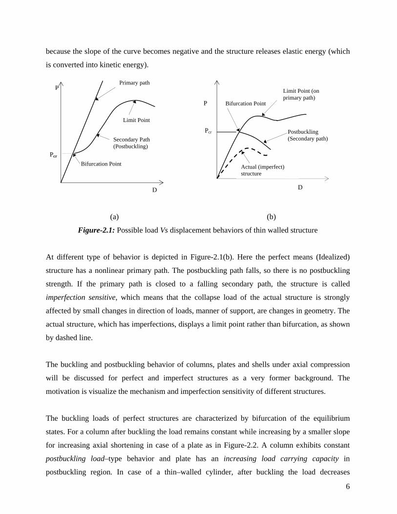
because the slope of the curve becomes negative and the structure releases elastic energy (which

is converted into kinetic energy).

6

(a) (b)

Figure-2.1: Possible load Vs displacement behaviors of thin walled structure

At different type of behavior is depicted in Figure-2.1(b). Here the perfect means (Idealized)

structure has a nonlinear primary path. The postbuckling path falls, so there is no postbuckling

strength. If the primary path is closed to a falling secondary path, the structure is called

imperfection sensitive, which means that the collapse load of the actual structure is strongly

affected by small changes in direction of loads, manner of support, are changes in geometry. The

actual structure, which has imperfections, displays a limit point rather than bifurcation, as shown

by dashed line.

The buckling and postbuckling behavior of columns, plates and shells under axial compression

will be discussed for perfect and imperfect structures as a very former background. The

motivation is visualize the mechanism and imperfection sensitivity of different structures.

The buckling loads of perfect structures are characterized by bifurcation of the equilibrium

states. For a column after buckling the load remains constant while increasing by a smaller slope

for increasing axial shortening in case of a plate as in Figure-2.2. A column exhibits constant

postbuckling load–type behavior and plate has an increasing load carrying capacity in

postbuckling region. In case of a thin–walled cylinder, after buckling the load decreases

Pcr

Bifurcation Point

Postbuckling (Secondary path)

Limit Point (on primary path)

Actual (imperfect) structure

D

P

Pcr

D

P

Limit Point

Secondary Path (Postbuckling)

Bifurcation Point

Primary path

7

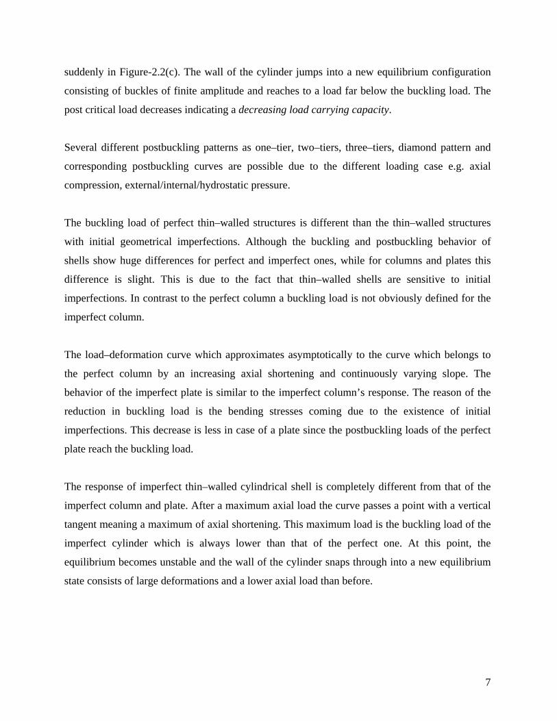
suddenly in Figure-2.2(c). The wall of the cylinder jumps into a new equilibrium configuration

consisting of buckles of finite amplitude and reaches to a load far below the buckling load. The

post critical load decreases indicating a decreasing load carrying capacity.

Several different postbuckling patterns as one–tier, two–tiers, three–tiers, diamond pattern and

corresponding postbuckling curves are possible due to the different loading case e.g. axial

compression, external/internal/hydrostatic pressure.

The buckling load of perfect thin–walled structures is different than the thin–walled structures

with initial geometrical imperfections. Although the buckling and postbuckling behavior of

shells show huge differences for perfect and imperfect ones, while for columns and plates this

difference is slight. This is due to the fact that thin–walled shells are sensitive to initial

imperfections. In contrast to the perfect column a buckling load is not obviously defined for the

imperfect column.

The load–deformation curve which approximates asymptotically to the curve which belongs to

the perfect column by an increasing axial shortening and continuously varying slope. The

behavior of the imperfect plate is similar to the imperfect column’s response. The reason of the

reduction in buckling load is the bending stresses coming due to the existence of initial

imperfections. This decrease is less in case of a plate since the postbuckling loads of the perfect

plate reach the buckling load.

The response of imperfect thin–walled cylindrical shell is completely different from that of the

imperfect column and plate. After a maximum axial load the curve passes a point with a vertical

tangent meaning a maximum of axial shortening. This maximum load is the buckling load of the

imperfect cylinder which is always lower than that of the perfect one. At this point, the

equilibrium becomes unstable and the wall of the cylinder snaps through into a new equilibrium

state consists of large deformations and a lower axial load than before.

Figure-2.2: Prebuckling and postbuckling of perfect and imperfect structures

In the buckling process, the difference between the buckling pattern and the postbuckling pattern

should be distinguished. The radial displacements of the buckling pattern are infinitesimally

small and can not be seen by naked eye. Moreover the buckling pattern is usually unstable.

Therefore as soon as the buckling load is reached, the shell snaps into a stable periodic

postbuckling pattern with visible buckles of finite depth.

2.3. Imperfection Sensitivity: In reality many shells fail at a smaller load than the theoretical critical load. The reason of this

early collapse is the effect of small, unavoidable geometrical imperfections. After reaching the

critical states, the load rapidly decreases while deflections increases meaning that the structure

undergoes softening. Furthermore a small disturbance can cause the shell to jump to a

postbuckling state at which the carrying capacity is greatly reduced. Imperfections may come

from

8

• The fact that no member of a structure can be constructed perfectly.

• The inability to ensure that the load actually act geometrically perfect.

In Fig. 2.2 (a–c) the load is plotted against the buckling displacement w which is

perpendicular to the shell surface. Fig. 2.2 (a) shows that after reaching the critical load, the load

carrying capacity of the axially compressed structure remains constant. Initial imperfections

increase the deformations, but curves will have no peak points, approaching to the horizontal line

of the perfect one asymptotically.

xN

Fig. 2.2 (b) shows the increasing load carrying capacity in the postbuckling region. In case of a

perfect plate there is a definite critical load at which buckling occurs but for an imperfect plate

there exists no certainly defined critical buckling load. The buckling deformation increases with

increasing load. As a consequence this structure is imperfection–insensitive.

For axially compressed cylinders described in Fig. 2.2 (c), the load carrying capacity decreases

after reaching a certain critical load and snaps through a lower load level. These kinds of

structures are very imperfection–sensitive.

As Koiter showed that the imperfection sensitivity of cylindrical shell structures is closely

related with their initial postbuckling behavior. In case of a plate, i.e. when early postbuckling

path has a positive curvature the structure is able to develop considerable postbuckling strength,

and loss of stability of the primary path does not result in structural collapse as in Fig. 2.2 (b).

For a cylinder which has a negative slope in the initial postbuckling region, buckling will occur

violently and buckling load depends on the initial imperfections. Consequently, sensitivity of the

structure to imperfections is affected by early postbuckling behavior and the shape of the

postbuckling equilibrium path plays a central role in determining the influence of initial

imperfections.

Thicker shells appear to be less sensitive to imperfections than thinner shells. As the structure

becomes thinner the sensitivity to imperfections increases. Shells subjected to external pressure

are less sensitive to imperfections than are shells subjected to axial compression because the

wave lengths of buckles in axial direction are longer in the former case and eigenvalues do not

cluster around the critical value. Hence, very small local imperfections do not affect the critical

pressure as much as they affect the critical axial load and, a very small local imperfection can

tend to trigger premature failure. One of the reasons of high imperfection sensitivity of these

highly symmetrical systems comes from the facts that many different buckling modes are

associated with more or less same eigenvalues. For simulations of imperfect shells it is an

9

10

important issue to decide about the imperfection amplitude and form to simulate an almost real

behavior. Initial geometric imperfections can be either axi-symmetric or asymmetric and either

in shape of classical buckling mode or in shape of diamond buckling pattern and as combinations

of different possibilities.

3. Construction Details

At first it is required to develop a mechanical model for the steel glass roofing by abstraction of

the real roof to its significant structural elements. To reduce the computational effort it is

required to simplify the model as much as possible, but without disregarding important

characteristics of the basic system.

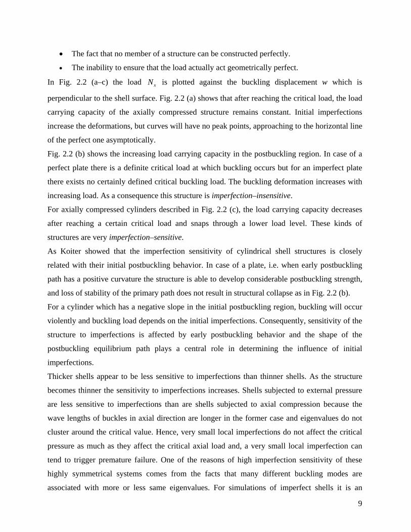
3.1. Geometrical details: In the Figure-3.1 we can see the architectural design of the gymnasium in Halstenbek, Germany.

The glass roofing has an elliptical horizontal projection with a length of 46m and a width of 28m.

The shell structure is parabolic in both directions with a height of 4.6m. The roof is composed of

shallow steel arches at intervals of about 1.2m and prestressed steel cables, which are diagonal,

and attached to arches as well as the glass elements, which form the exterior shell.

Figure-3.1: Architectural design of gymnasium in Halstenbek, Germany

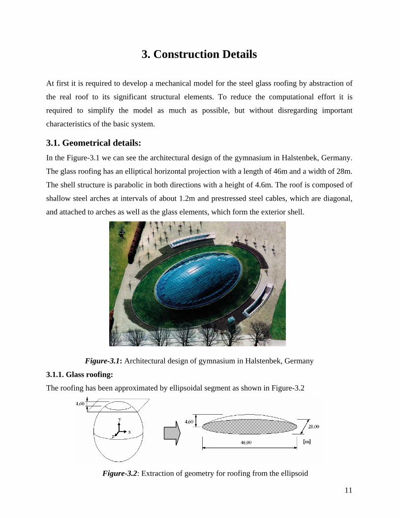
3.1.1. Glass roofing:

The roofing has been approximated by ellipsoidal segment as shown in Figure-3.2

Figure-3.2: Extraction of geometry for roofing from the ellipsoid

11

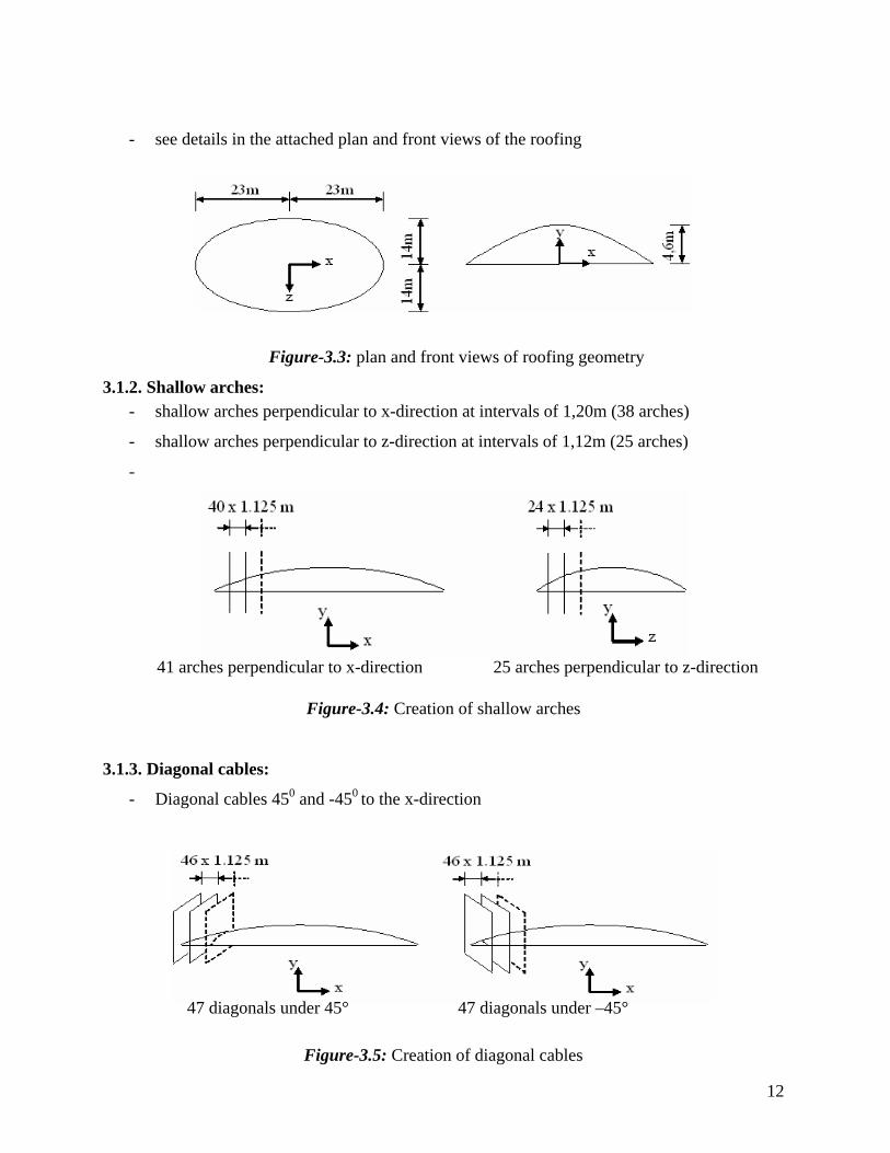
- see details in the attached plan and front views of the roofing

Figure-3.3: plan and front views of roofing geometry

3.1.2. Shallow arches: - shallow arches perpendicular to x-direction at intervals of 1,20m (38 arches)

- shallow arches perpendicular to z-direction at intervals of 1,12m (25 arches)

-

41 arches perpendicular to x-direction 25 arches perpendicular to z-direction

Figure-3.4: Creation of shallow arches

3.1.3. Diagonal cables:

- Diagonal cables 450 and -450 to the x-direction

47 diagonals under 45° 47 diagonals under –45°

Figure-3.5: Creation of diagonal cables

12

3.1.4. Types of Joints:

In the nonlinear and stability analysis of this shallow shell structure we are considering three

types of joints for horizontal and vertical shallow arches with the prestressing cables:

Joint-1: Bending resistant joints

Joint-2: pin joints

Joint-3: joints with decreased stiffness

Pin-jointed truss elements Bending resistant jointed beam elements:

Joints with decreased stiffness:

Figure-3.6: schematic representation of type of joints used in the mechanical model

3.2. Support conditions: - surrounding basic beam is sliding supported on concrete shell substructure in vertical

direction at intervals of 1.2-1.5 m; the basic beam can not rotate in the supports

- in horizontal direction the surrounding basic beam is supported only in angular points

- see support conditions in Figure-6

Figure-3.7: schematic representation of support conditions 13

3.3. Material and geometrical dimensions of components:

- shallow arch elements: flat bar: Steel S 355 decreased stiffness

(Rectangular section) dimensions: 40 x 60 [mm] joints: 2 x 60 x 7.5

A = 2400 mm² A ’= 900 mm²

zI = 720000 mm4 ’= 270000 mmzI 4

yI = 320000 mm4 ’= 241900 mmyI 4

TI = 755000 mm4 (Schlaich) E = 210000 N/mm² ’= 4220 mmyI 4

yσ = 360 N/mm² (Reiss)

ν = 0.3 ρ = 7850 kg/m³

Tα = 1.2.10-5 K

- basis beam: flat bar: Steel S 355 (Rectangular section) dimensions: 220 x 40 [mm]

A = 8800 mm²

zI = 1170000 mm4

yI = 35490000 mm4

TI = 125430000 mm4

E = 210000 N/mm²

yσ = 360 N/mm²

ν = 0.3 ρ = 7850 kg/m³

Tα = 1.2.10-5 K

- steel cable: 1 x 37 lacing dimensions: 2 x ∅6 [mm] A = 44.8 mm² E = 160000 N/mm²

yσ = 1570 N/mm²

ρ = 7850 kg/m³

Tα = 1.2.10-5 K prestress =800

14

- glass roof: = 18 mm (thickness) tE = 70000 N/mm² ν = 0.23 ρ = 2500 kg/m³

Tα = 0.9.10-5 K

3.4. Loading: (according to German standard)

- Load case 1: dead load shallow arch elements: G = 78.5 kN/m³. 0.04 m. 0.06 m = 0.1884kN/m g = 2. 0.1884kN/m / 1.20 m = 0.314 kN/m² steel cable: G = 78.5 kN/m³. 44.8. 10-6 = 0.0035kN/m g = 2. [0.0035kN/m. ( 2 . 1.2 m)] / (1.2 m)² = 0.008 kN/m² glass roof: g = 25 kN/m³. 0,018 m = 0.450 kN/m²

sum: 0.772 kN/m²

2% addition for small parts: 1.02. 0.774 kN/m² = 0.788 kN/m²

- Load case 2: wind (simplified)

Compression coefficient cp:

Figure-3.8: simplified wind loading case considered in the analysis

building height above site: < 8 m

impact pressure: q = 0.5kN/m² circumscribed rectangle ground plan: h/b < 5; h/a < 5

force coefficient: cf = 1.3

15

16

compression: qw = 0.3. cf. q = 0.195kN/m² suction : qw = 0.7. cf. q = 0.455kN/m²

- Imperfections:

applied according to eigenforms

- Load combination : dead load + wind

1.35. dead load + 1.5. wind

4. Finite Element Discretization of Shell Structure

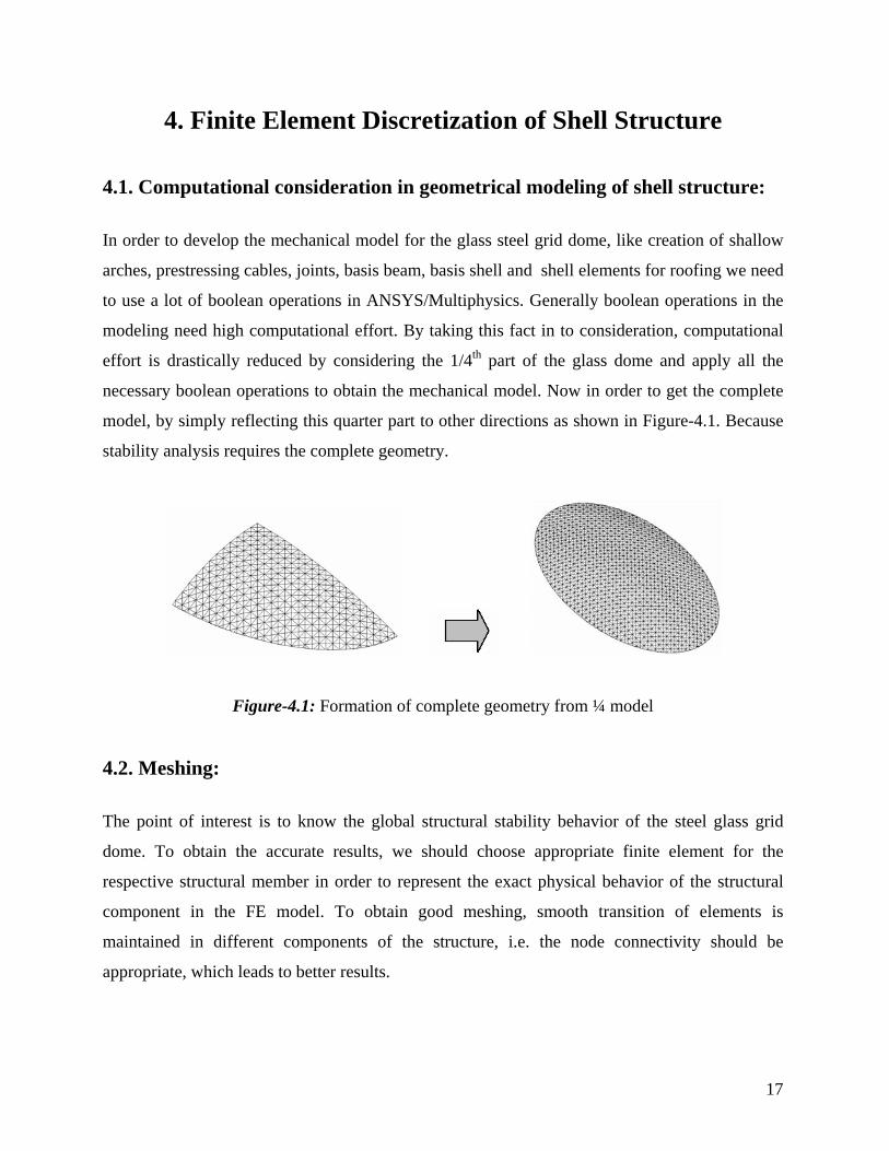
4.1. Computational consideration in geometrical modeling of shell structure:

In order to develop the mechanical model for the glass steel grid dome, like creation of shallow

arches, prestressing cables, joints, basis beam, basis shell and shell elements for roofing we need

to use a lot of boolean operations in ANSYS/Multiphysics. Generally boolean operations in the

modeling need high computational effort. By taking this fact in to consideration, computational

effort is drastically reduced by considering the 1/4th part of the glass dome and apply all the

necessary boolean operations to obtain the mechanical model. Now in order to get the complete

model, by simply reflecting this quarter part to other directions as shown in Figure-4.1. Because

stability analysis requires the complete geometry.

Figure-4.1: Formation of complete geometry from ¼ model

4.2. Meshing:

The point of interest is to know the global structural stability behavior of the steel glass grid

dome. To obtain the accurate results, we should choose appropriate finite element for the

respective structural member in order to represent the exact physical behavior of the structural

component in the FE model. To obtain good meshing, smooth transition of elements is

maintained in different components of the structure, i.e. the node connectivity should be

appropriate, which leads to better results.

17

18

4.2.1. Basis Beam & Shallow arches (BEAM4):

BEAM4 might be a suitable element for nonlinear and buckling finite element modeling of Basis

beam and Shallow arches, because it is a uniaxial element with tension, compression, torsion,

and bending capabilities. The element has six degrees of freedom at each node: translations in

the nodal x, y, and z directions and rotations about the nodal x, y, and z axes. Stress stiffening

and large deflection capabilities are included. A consistent tangent stiffness matrix option is

available for use in large deflection analyses.

4.2.2. Prestressed Cables (LINK10):

LINK10 element could be best suitable for FE modeling of prestressing cables. LINK10 is a

three-dimensional spar element having the unique feature of a bilinear stiffness matrix resulting

in a uniaxial tension-only (or compression-only) element. With the tension-only option, the

stiffness is removed if the element goes into compression (simulating a slack cable or slack chain

condition). This feature is useful for static cable wire applications where the entire cable wire is

modeled with one element. LINK10 has three degrees of freedom at each node: translations in

the nodal x, y, and z directions. No bending stiffness is included in either the tension-only (cable)

option or the compression-only (gap) option. The element is not capable of carrying bending

loads. The stress is assumed to be uniform over the entire element.

4.2.3. Glass Dome of the Structure (SHELL43):

SHELL43could be well suited to model the Shallow Shell member, because it is used for linear,

warped, moderately-thick shell structures. The element has six degrees of freedom at each node:

translations in the nodal x, y, and z directions and rotations about the nodal x, y, and z axes. The

deformation shapes are linear in both in-plane directions. For the out-of-plane motion, it uses a

mixed interpolation of tensorial components. The element has plasticity, creep, stress stiffening,

large deflection, and large strain capabilities.

4.2.4. Pin Jointed Truss Elements (LINK8):

In the case of pin jointed structures, we are assuming that the structural members do not carry the

bending loads. In such situations, LINK8 could be the best choice. LINK8 is a spar which may

be used in a variety of engineering applications. This element can be used to model trusses,

sagging cables, links, springs, etc. The three-dimensional spar element is a uniaxial tension-

compression element with three degrees of freedom at each node: translations in the nodal x, y,

and z directions. The element is not capable of carrying bending loads. The stress is assumed to

be uniform over the entire element.

Figure-4.2: Discretized model of shell structure

4.3. Boundary Conditions: An accurate modelling of the boundary conditions is very important in order to get the

correct results from the FE-analysis. The boundary conditions should be modelled as close to

the real-life situation as possible. In order to predict the global structural stability behaviour

of the shell structure, applied support conditions are as follows. Surrounding basic beam is

sliding supported on concrete shell substructure in vertical direction at intervals of 1.2-1.5 m,

and the basic beam can not rotate in the supports and in horizontal direction the surrounding

basic beam is supported only in angular points as shown in Figure-

Figure-4.3: Support conditions applied to shell structure

19

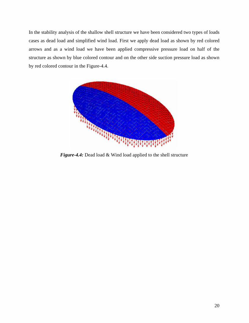
In the stability analysis of the shallow shell structure we have been considered two types of loads

cases as dead load and simplified wind load. First we apply dead load as shown by red colored

arrows and as a wind load we have been applied compressive pressure load on half of the

structure as shown by blue colored contour and on the other side suction pressure load as shown

by red colored contour in the Figure-4.4.

Figure-4.4: Dead load & Wind load applied to the shell structure

20

5. Numerical Simulation of Shell Buckling

Within the last decade, it is reviewed that, with the evaluation of finite element analysis of

stability problems, the advance of powerful computers and highly competent numerical

techniques has come to a state where any given shell structure can be calculated—no matter how

complicated the geometry, how dominant the imperfection influence and how nonlinear the load

carrying behavior is. However, the main task of the design engineer is, more than ever, to model

his shell problem properly and to convert the numerical output into the characteristic buckling

strength of the “real” shell which is needed for an equally safe and economic design.

The following observations are concerned with different kinds of numerical approaches to shell

buckling when using a commercial FEM package like ANSYS. 5.1. Eigenvalue buckling analysis:

Eigenvalue buckling analysis predicts the theoretical buckling strength (the bifurcation point) of

an ideal linear elastic structure. This method corresponds to the textbook approach to elastic

buckling analysis: for instance, an eigenvalue buckling analysis of a column will match the

classical Euler solution. However, imperfections and nonlinearities prevent most real-world

structures from achieving their theoretical elastic buckling strength. Thus, eigenvalue buckling

analysis often yields unconservative results, and should generally not be used in actual day-to-

day engineering analyses. The appropriate eigenvectors { }iψ are representing the buckling

shapes (deformation pattern which is characterizing the alternative response paths). These

eigenvectors are giving qualitative information about the buckling shape but not quantitative

information. This restriction to qualitative information is a fundamental characteristic of

eigenvalue problems.

The lowest eigenvalue load of the perfect shell is needed as critical buckling resistance for

the simplest numerically based design approach. It is generally no problem to produce this

eigenvalue for a given FE model. However, it should be very cautious about the elementary

mistakes which are made again and again when defining the FE model of a given shell buckling,

such as the level of discretization i.e. the number of finite elements used in the analysis, type of

boundary conditions, loading cases etc,.

crP

21

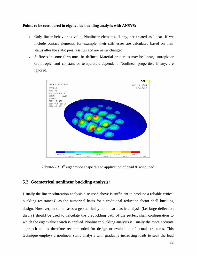
Points to be considered in eigenvalue buckling analysis with ANSYS:

• Only linear behavior is valid. Nonlinear elements, if any, are treated as linear. If we

include contact elements, for example, their stiffnesses are calculated based on their

status after the static prestress run and are never changed.

• Stiffness in some form must be defined. Material properties may be linear, isotropic or

orthotropic, and constant or temperature-dependent. Nonlinear properties, if any, are

ignored.

Figure-5.1: 1st eigenmode shape due to application of dead & wind load

5.2. Geometrical nonlinear buckling analysis:

Usually the linear bifurcation analysis discussed above is sufficient to produce a reliable critical

buckling resistance as the numerical basis for a traditional reduction factor shell buckling

design. However, in some cases a geometrically nonlinear elastic analysis (i.e. large deflection

theory) should be used to calculate the prebuckling path of the perfect shell configuration to

which the eigenvalue search is applied.

crP

Nonlinear buckling analysis is usually the more accurate

approach and is therefore recommended for design or evaluation of actual structures. This

technique employs a nonlinear static analysis with gradually increasing loads to seek the load

22

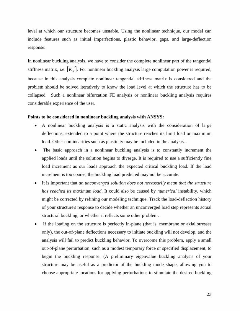
level at which our structure becomes unstable. Using the nonlinear technique, our model can

include features such as initial imperfections, plastic behavior, gaps, and large-deflection

response.

23

]In nonlinear buckling analysis, we have to consider the complete nonlinear part of the tangential

stiffness matrix, i.e. [ . For nonlinear buckling analysis large computation power is required,

because in this analysis complete nonlinear tangential stiffness matrix is considered and the

problem should be solved iteratively to know the load level at which the structure has to be

collapsed. Such a nonlinear bifurcation FE analysis or nonlinear buckling analysis requires

considerable experience of the user.

NK

Points to be considered in nonlinear buckling analysis with ANSYS:

• A nonlinear buckling analysis is a static analysis with the consideration of large

deflections, extended to a point where the structure reaches its limit load or maximum

load. Other nonlinearities such as plasticity may be included in the analysis.

• The basic approach in a nonlinear buckling analysis is to constantly increment the

applied loads until the solution begins to diverge. It is required to use a sufficiently fine

load increment as our loads approach the expected critical buckling load. If the load

increment is too coarse, the buckling load predicted may not be accurate.

• It is important that an unconverged solution does not necessarily mean that the structure

has reached its maximum load. It could also be caused by numerical instability, which

might be corrected by refining our modeling technique. Track the load-deflection history

of your structure's response to decide whether an unconverged load step represents actual

structural buckling, or whether it reflects some other problem.

• If the loading on the structure is perfectly in-plane (that is, membrane or axial stresses

only), the out-of-plane deflections necessary to initiate buckling will not develop, and the

analysis will fail to predict buckling behavior. To overcome this problem, apply a small

out-of-plane perturbation, such as a modest temporary force or specified displacement, to

begin the buckling response. (A preliminary eigenvalue buckling analysis of your

structure may be useful as a predictor of the buckling mode shape, allowing you to

choose appropriate locations for applying perturbations to stimulate the desired buckling

response.) The imperfection (perturbation) induced should match the location and size of

that in the real structure. The failure load is very sensitive to these parameters.

Figure-5.2: Nonlinear buckling shape due to dead load of the structure

Figure-5.3: Nonlinear buckling shape due to dead & wind load on the structure

24

25

5.3. Nonlinear analysis of the imperfect shell: An “exact” FE analysis of the shallow shell configuration, i.e. including all nonlinear geometry,

support conditions and loading influences, but with perfect geometry, has become quite popular

among researchers. The reasons are in the author’s view: it is a challenge to master all the

complicated nonlinear techniques; the computational power to achieve this is available these

days; and the unpleasant problems of realistic imperfections are avoided. However, real shell

structures are imperfect—unfortunately.

From the foregoing explanations it may be concluded that, for a specific design case, a fully

nonlinear analysis of the perfect shell is physically reasonable only for a relatively thick-walled

shell for which a pronouncedly yield-induced collapse mechanism is expected.

The behavior of an imperfect shell can only be simulated by analyzing the imperfect shell itself.

However, this logical perception leads inevitably to the question of how the imperfections of a

real shell structure look. Without going into any detail, it may be stated that, no matter how

sophisticated a numerical imitation of an imperfection field may be, it still represents merely a

“substitute imperfection” because certain components of the real imperfections (e.g. residual

stresses, inhomogenities, anisotropies, loading and boundary inaccuracies) are eventually not

included and must therefore be “substituted” in the simulated imperfection model. Usually these

substitute imperfections are introduced in the form of equivalent geometric imperfections. In

literature numerous techniques are published by so many researchers on how to consider the

imperfections in numerical simulations.

Among all of these techniques, in our nonlinear imperfection simulations, worst geometric

imperfections technique has been considered. The idea to find the “worst possible” geometric

imperfection pattern for a given, to-be-designed shell structure and to introduce it into the

nonlinear analysis is as old as the discovery of the detrimental influence of imperfections. It was

common practice from the beginning, supposedly taken over from column and plate buckling

experience, to consider that imperfection pattern to be the worst which is affine to the lowest

eigenmode.

Figure-5.4: Deflection plot due to applied symmetric imperfection on dead load case

Figure-5.5: Deflection plot due to applied symmetric imperfection on dead & wind load case

26

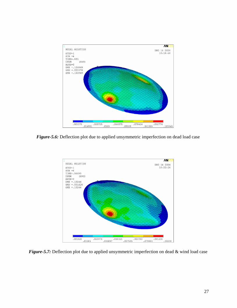
Figure-5.6: Deflection plot due to applied unsymmetric imperfection on dead load case

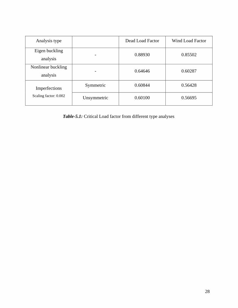
Figure-5.7: Deflection plot due to applied unsymmetric imperfection on dead & wind load case

27

28

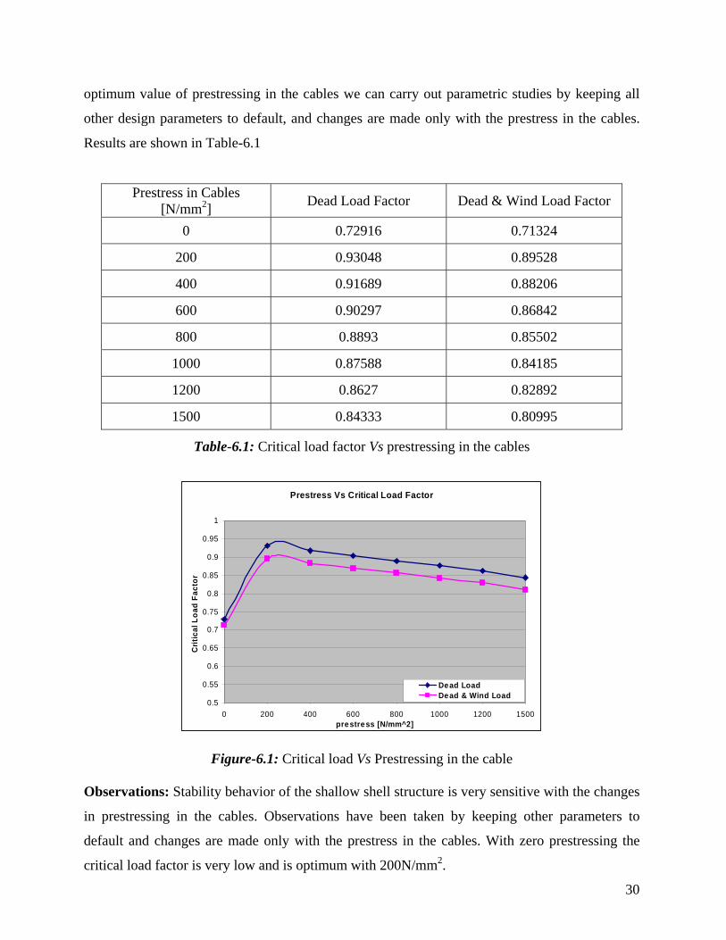
Analysis type Dead Load Factor Wind Load Factor

Eigen buckling

analysis - 0.88930 0.85502

Nonlinear buckling

analysis - 0.64646 0.60287

Symmetric 0.60844 0.56428 Imperfections Scaling factor: 0.002 Unsymmetric 0.60100 0.56695

Table-5.1: Critical Load factor from different type analyses

29

6. Investigation of Stability Behavior due to Changes

in Design Parameters

In reality the gymnasium located in Halstenbek, Germany which we considered in our

simulations, was collapsed two times. First collapse was happened at construction stage. Reason

for this collapse was, that the diagonal cables were partially installed, but not prestressed which

leads to unstable state of glass grid dome during a normal storm. So the steel frame requires a

large number of temporary columns to support the structure in the assembly state. But in reality

only 10% of the flat bar joints were supported and this fact led to large imperfections, structure

was not able to resist moderate wind loads and was collapsed during a storm.

The second collapse occurred when the glass roofing was completely built. Investigations of

experts in structural design reveal that, the failure of the structure is mainly due to the following

reasons:

• Unfavourable support conditions for the membrane shell, which leads to no equilibrium

of forces. In reality vertical support was used. But in an ideal membrane we have only

normal forces. Because of this vertical support, we obtain a reaction force component

perpendicular to the membrane layer, which is therewith not in equilibrium.

• Reduced stiffness in joints, because of smaller cross sectional area of mounting links

which leads to lower bending stiffness in the joints.

• Imperfections which were distributed over the complete structure and exceeded the

tolerances, which leads to decrease in ultimate load of roofing.

From the foregoing discussions it may be concluded that, the structure was collapsed due to

unfavorable design parameters of the structure. During this work, we have been trying to

optimize the design of glass roofing of gymnasium in Halstenbek with the reasonable changes in

support conditions, prestressing in the cables, stiffness in joints, stiffness in basis beam and arch

rise of the shell.

6.1. Sensitivity of stability behavior due to changes in prestressing in cables: The application of load to a structure so as to deform it in such a manner that the structure will

withstand its working load more effectively or with less deflection is called prestressing a

structure. We can able to increase the stability of the steel shell structure, by the application of

prestressing in the cables, which are attached to the steel shallow arches. To finding out the

optimum value of prestressing in the cables we can carry out parametric studies by keeping all

other design parameters to default, and changes are made only with the prestress in the cables.

Results are shown in Table-6.1

Prestress in Cables [N/mm2] Dead Load Factor Dead & Wind Load Factor

0 0.72916 0.71324

200 0.93048 0.89528

400 0.91689 0.88206

600 0.90297 0.86842

800 0.8893 0.85502

1000 0.87588 0.84185

1200 0.8627 0.82892

1500 0.84333 0.80995

Table-6.1: Critical load factor Vs prestressing in the cables

Prestress Vs Critical Load Factor

0.5

0.55

0.6

0.65

0.7

0.75

0.8

0.85

0.9

0.95

1

0 200 400 600 800 1000 1200 1500prestress [N/mm^2]

Crit

ical

Loa

d Fa

ctor

Dead LoadDead & Wind Load

Figure-6.1: Critical load Vs Prestressing in the cable

Observations: Stability behavior of the shallow shell structure is very sensitive with the changes

in prestressing in the cables. Observations have been taken by keeping other parameters to

default and changes are made only with the prestress in the cables. With zero prestressing the

critical load factor is very low and is optimum with 200N/mm2.

30

6.2. Sensitivity of stability behavior due to changes in bending stiffness of the joints:

Dimensions [mm] Area[mm2] Iy[*1000m

m4] Iz[*1000m

m4] Dead Load Dead & Wind

L = 60 B = 7.5 900 241 270 0.88930 0.85502

L = 60 B = 9.375 1125 333.4 337.5 0.92727 0.89305

L = 75 B = 7.5 1125 302 527 0.94562 0.91130

L = 80 B = 7.5 1200 322.5 640 0.96844 0.93470

L = 75 B = 9.375 1406 417 659 0.98246 0.94907

L = 80 B = 9.375 1500 444.5 800 0.99561 0.96215

L = 85 B = 10.5 1785 547 1075 1.0173 0.98378

L = 90 B = 10.5 1890 596 1276 1.0271 0.99349

Table-6.2: Critical load Vs Stiffness in the joints

Critical Load Factor Vs Bending Stiffness (Z-direction) in Joints

0.80

0.85

0.90

0.95

1.00

1.05

270 337 527 640 659 800 1075 1276

Bending Stiffness (*1000)

Criti

cal L

oad

Fact

or

Dead LoadDead & Wind Load

Figure-6.2: Critical load Vs Stiffness in the basis beam

Observations: The stability of the structure is very sensitive with the bending stiffness in the

joints. It is observed that for the same cross-sectional areas, the structure is more stable for

higher values of bending stiffness in z-direction i.e. length direction, compared with the stiffness

in width direction.

31

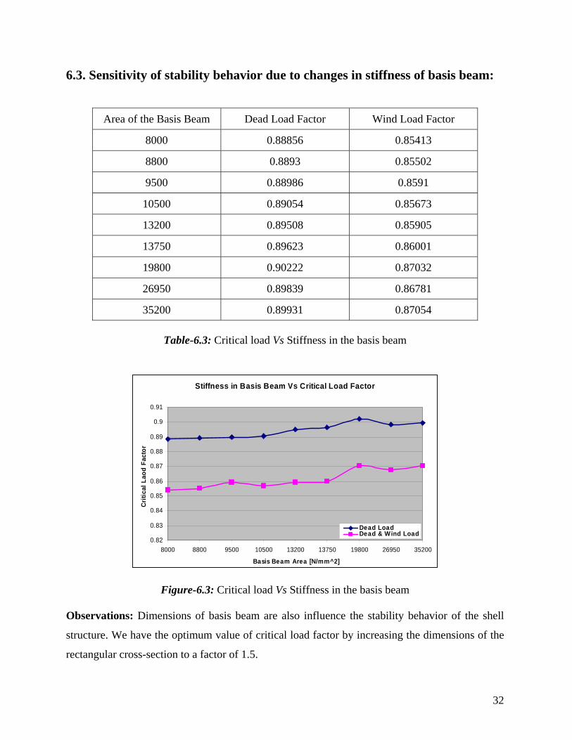
6.3. Sensitivity of stability behavior due to changes in stiffness of basis beam:

Area of the Basis Beam Dead Load Factor Wind Load Factor

8000 0.88856 0.85413

8800 0.8893 0.85502

9500 0.88986 0.8591

10500 0.89054 0.85673

13200 0.89508 0.85905

13750 0.89623 0.86001

19800 0.90222 0.87032

26950 0.89839 0.86781

35200 0.89931 0.87054

Table-6.3: Critical load Vs Stiffness in the basis beam

Stiffness in Basis Beam Vs Critical Load Factor

0.82

0.83

0.84

0.85

0.86

0.87

0.88

0.89

0.9

0.91

8000 8800 9500 10500 13200 13750 19800 26950 35200

Basis Beam Area [N/mm^2]

Crit

ical

Lao

d Fa

ctor

Dead LoadDead & Wind Load

Figure-6.3: Critical load Vs Stiffness in the basis beam

Observations: Dimensions of basis beam are also influence the stability behavior of the shell

structure. We have the optimum value of critical load factor by increasing the dimensions of the

rectangular cross-section to a factor of 1.5.

32

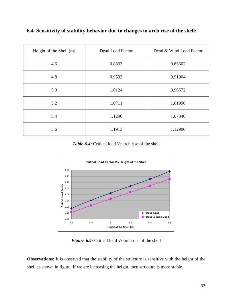
6.4. Sensitivity of stability behavior due to changes in arch rise of the shell:

Height of the Shell [m] Dead Load Factor Dead & Wind Load Factor

4.6 0.8893 0.85502

4.8 0.9533 0.91004

5.0 1.0124 0.96572

5.2 1.0711 1.01990

5.4 1.1296 1.07340

5.6 1.1913 1.12900

Table-6.4: Critical load Vs arch rise of the shell

Critical Load Factor Vs Height of the Shell

0.80

0.85

0.90

0.95

1.00

1.05

1.10

1.15

1.20

4.6 4.8 5 5.2 5.4 5.6

Height of the Shell [m]

Criti

cal L

oad

Fact

or

Dead Load Dead & Wind Load

Figure-6.4: Critical load Vs arch rise of the shell

Observations: It is observed that the stability of the structure is sensitive with the height of the

shell as shown in figure. If we are increasing the height, then structure is more stable.

33

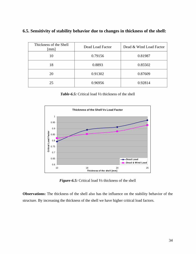
6.5. Sensitivity of stability behavior due to changes in thickness of the shell:

Thickness of the Shell [mm] Dead Load Factor Dead & Wind Load Factor

10 0.79156 0.81987

18 0.8893 0.85502

20 0.91302 0.87609

25 0.96956 0.92814

Table-6.5: Critical load Vs thickness of the shell

Thickness of the Shell Vs Load Factor

0.6

0.65

0.7

0.75

0.8

0.85

0.9

0.95

1

10 18 20 25Thickness of the shell [mm]

Cri

tical

Loa

d Fa

ctor

Dead LoadDead & Wind Load

Figure-6.5: Critical load Vs thickness of the shell

Observations: The thickness of the shell also has the influence on the stability behavior of the

structure. By increasing the thickness of the shell we have higher critical load factors.

34

35

6.6. Sensitivity of stability behavior due to application of geometric imperfections:

Type of Imperfection Scaling Factor Dead Load Dead & Wind Load

0.002 0.608442 0.56428 Symmetrical

0.01 0.51909 0.46242

0.002 0.60100 0.56695 Unsymmetrical

0.01 0.49938 0.48100

With out Imperfection - 0.60287 0.64646

Table-6.6: Application of geometric imperfections

Observations:

1. Load factor decrease with increases in Imperfection

2. Max deflection increases in case of symmetric loading with symmetric imperfection

increases as in case of Dead load case

3. With wind , the result is difficult to predict (unsymmetrical imperfections)

4. Imperfection plays a vital role in determining the critical load

5. Imperfection should be included in the stability analysis of the structure

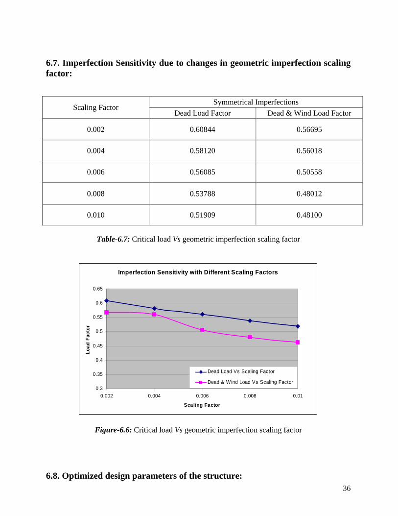
6.7. Imperfection Sensitivity due to changes in geometric imperfection scaling factor:

Symmetrical Imperfections Scaling Factor

Dead Load Factor Dead & Wind Load Factor

0.002 0.60844 0.56695

0.004 0.58120 0.56018

0.006 0.56085 0.50558

0.008 0.53788 0.48012

0.010 0.51909 0.48100

Table-6.7: Critical load Vs geometric imperfection scaling factor

Imperfection Sensitivity with Different Scaling Factors

0.3

0.35

0.4

0.45

0.5

0.55

0.6

0.65

0.002 0.004 0.006 0.008 0.01

Scaling Factor

Load

Fac

tor

Dead Load Vs Scaling Factor

Dead & Wind Load Vs Scaling Factor

Figure-6.6: Critical load Vs geometric imperfection scaling factor

6.8. Optimized design parameters of the structure: 36

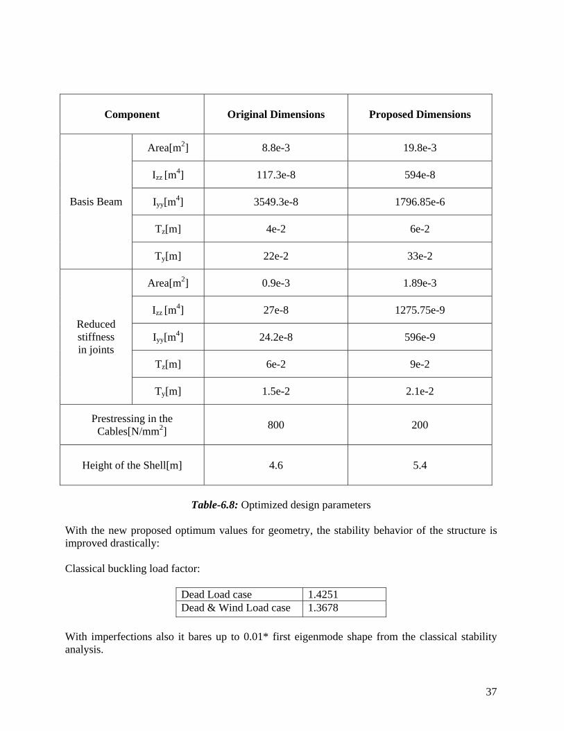
37

Component Original Dimensions Proposed Dimensions

Area[m2] 8.8e-3 19.8e-3

Izz [m4] 117.3e-8 594e-8

Iyy[m4] 3549.3e-8 1796.85e-6

Tz[m] 4e-2 6e-2

Basis Beam

Ty[m] 22e-2 33e-2

Area[m2] 0.9e-3 1.89e-3

Izz [m4] 27e-8 1275.75e-9

Iyy[m4] 24.2e-8 596e-9

Tz[m] 6e-2 9e-2

Reduced stiffness in joints

Ty[m] 1.5e-2 2.1e-2

Prestressing in the Cables[N/mm2] 800 200

Height of the Shell[m] 4.6 5.4

Table-6.8: Optimized design parameters

With the new proposed optimum values for geometry, the stability behavior of the structure is improved drastically: Classical buckling load factor:

Dead Load case 1.4251 Dead & Wind Load case 1.3678

With imperfections also it bares up to 0.01* first eigenmode shape from the classical stability analysis.

38

Conclusions

In the present work, static buckling of shell structures including eigenvalue buckling, nonlinear

buckling and imperfection sensitivity due to applied load, support conditions, stiffness in joints

and prestressing in the cables are discussed. Finally the design has been optimized with

reasonable design parameters: Optimum values for the design parameters have been obtained by

keeping other parameters to default and changes are only made with in the required design

parameter. It should keep in mind that, in this work all the calculations are carried out with the

assumption of linear elastic material behavior. So care should be taken while calculating the

optimum design parameters, since the stresses developed in the structural members may some

times crosses the yield point.

The prestressing in cables opens more advantages since the initial strain is anticipated and larger

stiffness is obtained. And also prestressing in the cables alters the compressive membrane forces

in to tensile; ultimately bending stiffness in the structure might effectively increase. It has been

observed that, with zero prestressing the critical load factor is very low and is optimum with

200N/mm2.

In a thin walled structure such as a shell, membrane stiffness is typically orders of magnitude

greater than bending stiffness. Accordingly, small membrane deformations can store a large

amount of strain energy, but comparatively large lateral deflections are needed to absorb this

energy in bending deformations leads to buckling failures. In reality, cross section at the joints is

very low; consequently bending stiffness in joints is also smaller and structure is prone to

stability failure. So by increasing the bending stiffness in joints and basis beam, stability has

been increased effectively.

The arch rise of the shell structure is also a very big influencing factor on the structural stability.

As we know shell can carry a large load if membrane action dominates over bending, so by

increasing the height of the shell we can get large membrane stiffness which leads to high snap

through point (critical point) for geometrically perfect structures.

Out look: Buckling of structures is in reality a dynamic process. It can physically be defined as

the collapse of structures under loads that are less than those causing material failures and

usually results in a sudden catastrophic collapse of the structure. As a result, it may be more

realistic to approach buckling and loss of stability from a dynamic point of view.

39

Appendix-A ANSYS Input Codes

1. Geometry Input File FINISH /CLEAR, START !***************Geometry Parameters***! a=72.20932139 !x-dimension of ellipsoid b=96.0 !y-dimension of ellipsoid c=43.95349998 !z-dimension of ellipsoid h=5.0 !height of ellipsoidal segment kz=24 !Number of shallow arches spanned perpendicular to z-direction decreased by one (must be even) kx=40 !Number of shallow arches spanned perpendicular to x-direction decreased by one (must be even) dx=23 !x-distance (in numbers of shallow arches) of starting diagonal cable e=1.125 ! Distance between arches /PREP7 !***Creation of shell surface by an ellipsoid***! sph4,,,1 vlscale,1,,,a,b,c,,,1 BLOCK,-a-1,a+1,-b-1,b-h,-c-1,c+1, vovlap,1,2 !*****Erasure of no longer used volumes, areas, lines and key points***! NUMCMP,AREA agen,2,7 vdele,all adele,1,10 NUMCMP,AREA asel,s,,,1 lsla,all cm,lines,line alls lsel,all lsel,u,,,lines ldele,all cmdele,lines alls lsel,all ksll,all cm,keypoints,kp alls ksel,all ksel,u,,,keypoints kdele,all cmdele,keypoints aplot numcmp,line !**************Creation of !/4 th geometry***************! k,,,b-h,, k,,,b-h,14 ASBW,1 wpro,,90,, wpro,,90,, wpro,,,-90 NUMCMP,AREA ASBW,ALL

NUMCMP,AREA ADELE,3,4 ADELE,1 WPCSYS,-1 /REPLOT numcmp,area asel,s,,,1 lsla,all cm,lines,line alls lsel,all lsel,u,,,lines ldele,all cmdele,lines alls lsel,all ksll,all cm,keypoints,kp alls ksel,all ksel,u,,,keypoints kdele,all cmdele,keypoints aplot numcmp,line !***Generation of shallow archs in x-direction !(longerarchs)***! rectng,-a,a,b-h-1,b+1 /replot agen,kz/2+1,2,,,,,e ADELE, 2, , ,1 NUMCMP,AREA *GET,NUMBER,AREA,,NUM,MAX asba,1,number,,delete,delte numcmp,area asba,number,1,,delete,delte numcmp,area asba,number,1,,delete,delte numcmp,area n=number-4 /replot *do,i,1,n, numcmp,area asba,number-1,1,,delete,delete numcmp,area *enddo !***Generation of shallow archs in z-direction (shorter archs)***! local,11,0,e*kx/2,,,,,90 wpcsys,-1 rectng,-c,c,b-h-1,b+1 agen,(kx/2)+1,NUMBER+1,,,,,-e *GET,NUMBER2,AREA,,NUM,MAX n=NUMBER2-NUMBER *DO,i,1,n asba,all,NUMBER+i,,delete,delete *ENDDO NUMCMP,AREA ADELE,22,,,1 alls /REPLOT

40

!**Creation of components for shallow arches in x- and z-direction***! csys,0 lsel,s,loc,y,b-h,b-h+0.01 cm,basis,line alls lsel,all lsel,u,,,basis *DO,i,-kz/2,kz/2 lsel,u,loc,z,e*i *ENDDO cm,lattice1,line alls lsel,all lsel,u,,,basis lsel,u,,,lattice1 cm,lattice2,line cmdele,basis alls !***Generation of diagonal cables***! !Cables in first direction! *GET,NUMBER2,AREA,,NUM,MAX local,12,0,e*dx,,,,,45 wpcsys,-1 rectng,-c*2,c*2,b-h-1,b+1 csys,0 agen,dx+1,22,,,-e *GET,NUMBER3,AREA,,NUM,MAX n=NUMBER3-NUMBER2 asba,all,22,,keep,delete *DO,i,1,n asba,all,NUMBER2+i,,keep,delete *ENDDO adele,241,,,1 numcmp,area !Erasure of no longer used areas! alls asel,all asel,u,,,1,NUMBER2 adele,all,,, alls aplot !Creation of component for diagonals in first direction! lsel,s,loc,y,b-h,b-h+0.01 cm,basis,line alls lsel,all lsel,u,,,basis lsel,u,,, lattice1 lsel,u,,, lattice2 cm,cable1_1,line cmdele,basis alls numcmp,area local,13,0,e*dx,,,,,-45 wpcsys,-1 rectng,-c*2,c*2,b-h-1,b+1 csys,0 agen,1.5*dx+1,NUMBER2+1,,,-e *DO,i,1,n+14 asba,all,NUMBER2+i,,keep,delete *ENDDO adele,219,221,,1 !******Erasure of no longer used areas!****! alls asel,all asel,u,,,1,NUMBER2 adele,all alls aplot

!Creation of component for shell areas! asel,all cm,shell1,area !Creation of component for diagonals in second direction! lsel,s,loc,y,b-h,b-h+0.01 cm,basis,line alls lsel,all lsel,u,,,basis lsel,u,,, lattice1 lsel,u,,, lattice2 lsel,u,,,cable1_1 lsel,u,,,1,2 cm,cable2_2,line cmdele,basis alls numcmp,line !***************************************************** !Generation of identical help geometry! agen,2,shell1,,,,-b !Creation of component for basis lines of shell areas! asel,s,,,shell1 lsla,all lsel,r,loc,y,b-h,b-h+0.01 cm,basis_shell1,line !Generation of diagonals in first direction within help geometry! alls numcmp,area *GET,NUMBER4,AREA,,NUM,MAX local,14,0,e*dx,-b,,,,45 wpcsys,-1 rectng,-c*2,c*2,b-h-1,b+1 csys,0 agen,dx+1,NUMBER4+1,,,-e alls *DO,i,1,n asba,all,NUMBER4+i,,delete,delete *ENDDO adele,460,,,1 !Generation of diagonals in second direction within help geometry! alls numcmp,area *GET,NUMBER5,AREA,,NUM,MAX local,15,0,e*dx,-b,,,,-45 wpcsys,-1 rectng,-c*2,c*2,b-h-1,b+1 csys,0 agen,1.5*dx+1,NUMBER5+1,,,-e alls *DO,i,1,n+14 asba,all,NUMBER5+i,,delete,delete *ENDDO adele,644,646,,1 numcmp,area !Erasure of no longer used lines in original geometry! lsel,s,loc,y,b-h,b-h+0.01 lsel,u,,,basis_shell1 ldele,all !Copying of new splitted basis lines into the original geometry! lsel,s,loc,y,-h,-h+0.01 lgen,2,all,,,,b !Creation of component for basis lines belonging to basis beam! lsel,s,loc,y,b-h,b-h+0.01 lsel,u,,,basis_shell1 cm,basis_beam1,line

41

alls !********Erasure of help geometry! asel,all asel,u,,,shell1 adele,all alls lsel,all lsel,u,,, lattice1 lsel,u,,, lattice2 lsel,u,,,cable1_1 lsel,u,,,cable2_2 lsel,u,,,basis_shell1 lsel,u,,,basis_beam1 ldele,all alls lplot !************Creation of Full geometry************** csys,0 lsel,s,loc,y,b-h,b-h+0.01 cm,basis,line alls kplo KSYMM,X,all, , , ,1,0 KSYMM,Z,all, , , ,1,0 lsel,all lsel,u,,,basis lsel,u,,, lattice2 lsel,u,,,cable1_1 lsel,u,,,cable2_2 LSYMM,X,all, , , ,1,0 LSYMM,Z,all, , , ,1,0 CM,arches1,LINE alls lsel,all lsel,u,,,basis lsel,u,,, lattice1 lsel,u,,,cable1_1 lsel,u,,,cable2_2 lsel,u,,,arches1 LSYMM,X,all, , , ,1,0 LSYMM,Z,all, , , ,1,0 CM,arches2,LINE alls lsel,all lsel,u,,,basis lsel,u,,, lattice1 lsel,u,,, lattice2 lsel,u,,,cable1_1 lsel,u,,,arches1 lsel,u,,,arches2 LSYMM,X,all, , , ,1,0 lsel,u,,,cable2_2 cm,a,line lsel,s,,,cable2_2 LSYMM,Z,all, , , ,1,0 lsel,u,,,cable2_2 cm,b,line lsel,s,,,a LSYMM,Z,all, , , ,1,0 lsel,u,,,a cm,c,line alls lsel,all lsel,u,,,basis lsel,u,,,lattice1 lsel,u,,,lattice2 lsel,u,,,cable2_2 lsel,u,,,arches1 lsel,u,,,arches2 lsel,u,,,a

lsel,u,,,b lsel,u,,,c LSYMM,X,all, , , ,1,0 Cmsel,u,cable1_1,line cm,d,line lsel,s,,,cable1_1 LSYMM,Z,all, , , ,1,0 lsel,u,,,cable1_1 cm,e,line lsel,s,,,d !lsel,u,,,cable1_1 LSYMM,Z,all, , , ,1,0 lsel,u,,,d cm,f,line lsel,a,,,a lsel,a,,,b lsel,a,,,cable1_1 cm,cable1,line cmdele,a cmdele,b cmdele,f alls lsel,all lsel,u,,,basis lsel,u,,,lattice1 lsel,u,,,lattice2 lsel,u,,,cable1_1 lsel,u,,,arches1 lsel,u,,,arches2 lsel,u,,,cable1 cm,cable2,line cmdele,c cmdele,d cmdele,e alls CMSEL,S,BASIS_BEAM1 LSYMM,X,all, , , ,1,0 LSYMM,Z,all, , , ,1,0 Cm,basis_beam,line CMSEL,S,BASIS_SHELL1 LSYMM,X,all, , , ,1,0 LSYMM,Z,all, , , ,1,0 Cm,basis_shell,line Cmdele,lattice1 Cmdele,lattice2 Cmdele,cable1_1 Cmdele,cable2_2 Cmdele,basis_beam1 Cmdele,basis_shell1 Cmdele,basis ! Cmdele,shell1 ARSYM,X,all, , , ,1,0 ARSYM,Z,all, , , ,1,0 Asel,all Cm,shell,area Alls Nummrg,kp Cmsel,s,arches1,line Cm,lattice1,line Cmsel,s,arches2,line Cm,lattice2,line Cmdele,arches1 Cmdele,arches2 Alls aplo FINISH

42

2. Discretization Input File: /PREP7 joint=2 !joint=0 ... bending resistant jointed !joint=1 ... pin-jointed !joint=2 ... joints with decreased stiffness shell=1 !shell=0 ... without shell elements !shell=1 ... with shell elements !***Material Parameters***! !***Units [kN],[m],[K]***! !******Basis Beam!*****! ET,1,BEAM4 KEYOPT,1,9,1 MP,EX,1,2.1e8 MP,NUXY,1,0.3 MP,ALPX,1,1.2e-5 MP,DENS,1,7.85 R,1,8.8e-3,117.3e-8,3549.3e-8,4e-2,22e-2 !Area,Izz,Iyy,Tz,Ty !******Shallow archs - Beam elements****! ET,2,BEAM4 KEYOPT,2,9,1 MP,EX,2,2.1e8 MP,NUXY,2,0.3 MP,ALPX,2,1.2e-5 MP,DENS,2,7.85 R,2,2.4e-3,72e-8,32e-8,6e-2,4e-2 !Area,Izz,Iyy,Tz,Ty !******Shallow arches - Link elements*****! ET,5,LINK8 MP,EX,5,2.1e8 MP,ALPX,5,1.2e-5 MP,DENS,5,7.85 R,5,2.4e-3 !Area !Shallow archs - Beam elements with decreased stiffness! R,6,0.9e-3,27e-8,24.2e-8,6e-2,1.5e-2 !Area,Izz,Iyy,Tz,Ty !******Prestressed Cables! ET,3,LINK10,,,0 !Keyopt(3)=0 ... Tension only MP,EX,3,1.6e8 MP,ALPX,3,1.2e-5 MP,DENS,3,7.85 R,3,44.8e-6,5e-3 !Area,InitialStrain !****Shell elements! ET,4,SHELL43 MP,EX,4,7e5 !MP,EX,4,7e7 MP,NUXY,4,0.23 MP,ALPX,4,0.9e-5 MP,DENS,4,2.5 R,4,1.8e-2 !Thickness !***Discretisation***! !******Basis Beam! alls lsel,s,,,basis_beam lesize,all,,,1 type,1 mat,1 real,1 lmesh,all esll,s cm,beam_el,elem alls !Shallow archs!

!********bending resistent jointed*********! *if,joint,eq,0,then lsel,s,,,lattice1 lsel,a,,,lattice2 lesize,all,,,1 type,2 mat,2 real,2 lmesh,all lsel,s,,,lattice1 lsel,a,,,lattice2 esll,s cm,lattice_el,elem alls *endif !***************pin-jointed****************! *if,joint,eq,1,then lsel,s,,,lattice1 lsel,a,,,lattice2 ksll,all ksel,r,loc,y,b-h,b-h+0.01 lslk,s,,,all lsel,u,,,basis_beam lsel,u,,,basis_shell cm,beam_line,line lesize,all,,,1 type,2 !bending resistant jointed basis beam joints mat,2 real,2 lmesh,all lsel,s,,,lattice1 lsel,a,,,lattice2 lsel,u,,,beam_line lesize,all,,,1 type,2 !pin jointed truss joints mat,2 real, lmesh,all cmdele,beam_line lsel,s,,,lattice1 lsel,a,,,lattice2 esll,s cm,lattice_el,elem alls *endif !*****joints with decreased stiffness******! *if,joint,eq,2,then lsel,s,,,lattice1 lsel,a,,,lattice2 ksll,all ksel,r,loc,y,b-h,b-h+0.01 lslk,s,,,all lsel,u,,,basis_beam lsel,u,,,basis_shell cm,beam_line,line lesize,all,,,1 type,2 !bending resistant jointed basis beam joints mat,2 real,2 lmesh,all esll,s cm,lowest_lattice_el,elem lsel,s,,,lattice1 lsel,a,,,lattice2 lsel,u,,,beam_line ldiv,all,0.1,,,0 cm,new_lines1,line lsel,r,length,,0,0.3 cm,joint_lines1,line lsel,s,,,new_lines1 lsel,u,,,joint_lines1

43

ldiv,all,0.91,,,0 cm,new_lines2,line lsel,r,length,,0,0.3 cm,joint_lines2,line lsel,s,,,new_lines2 lsel,u,,,joint_lines2 cm,middle_lines,line lsel,s,,,joint_lines1 lsel,a,,,joint_lines2 cm,joint_lines,line alls cmdele,joint_lines1 cmdele,joint_lines2 cmdele,new_lines1 cmdele,new_lines2 lsel,s,,,middle_lines lesize,all,,,1 type,2 mat,2 real,2 lmesh,all esll,s cm,lattice_el_middle,elem lsel,s,,,joint_lines lesize,all,,,1 type,2 mat,2 real,6 lmesh,all esll,s cm,lattice_el_joint,elem esel,s,,,lattice_el_middle esel,a,,,lattice_el_joint cm,remaining_lattice_el,elem esel,s,,,lowest_lattice_el esel,a,,,remaining_lattice_el cm,lattice_el,elem alls *endif !*************Spanned Cables********! lsel,s,,,cable1 lsel,a,,,cable2 lesize,all,,,1 type,3 mat,3 real,3 lmesh,all esll,s cm,cable_el,elem alls !********only for consideration of stiff shell elements*********! !*********Shell elements! *if,shell,eq,1,then asel,s,,,shell type,4 mat,4 real,4 esize,,1 amesh,all esla,s cm,shell_el,elem alls *endif !*********************************************! NUMMRG,NODE,0.0001, , ,LOW numcmp,node alls eplot FINISH

3. Boundary Conditions Input File /PREP7 !***Boundary Conditions***! Sup=0 !sup=0 ... vertical supported !sup=1 ... perpendicular to shell surface supported !sup=2 ... perpendicular and in shell surface dir. supported *if,sup,eq,0,then alls esel,s,,,lattice_el nsle,all nsel,r,loc,y,b-h-0.01,b-h+0.01 d,all,uy d,all,rotx d,all,rotz !smallest and highest x- and y-coordinate! nsel,r,loc,x,-0.01,0.01 d,all,ux esel,s,,,lattice_el nsle,all nsel,r,loc,y,b-h,b-h+0.01 nsel,r,loc,z,-0.01,0.01 d,all,uz *endif *if,sup,eq,1,or,sup,eq,2,then alls esel,s,,,lattice_el nsle,all nsel,r,loc,y,b-h-0.01,b-h+0.01 *GET,NUMBER,NODE,,COUNT *DO,ii,1,NUMBER *GET,Nr,NODE,,NUM,MIN *GET,xCor,NODE,Nr,LOC,X *GET,yCor,NODE,Nr,LOC,y *GET,zCor,NODE,Nr,LOC,Z *if,xCor,EQ,0,then n,100000,xCor+1,yCor,zCor *SET,y2,(1-(xCor)*xCor/(a*a)-(zCor+1)*zCor/(c*c))*b*b/yCor-yCor n,100001,xCor,yCor+y2,zCor+1 *else *if,zCor,EQ,0,then n,100000,xCor,yCor,zCor+1 *SET,y2,(1-(xCor+1)*xCor/(a*a)-(zCor)*zCor/(c*c))*b*b/yCor-yCor n,100001,xCor+1,yCor+y2,zCor *endif *if,zCor,GT,0,then *SET,z1,-14*xCor/(23*23)/SQRT(1-xCor*xCor/(23*23)) n,100000,xCor+1,yCor,zCor+z1 *SET,y2,(1-(xCor+1)*xCor/(a*a)-(zCor-1/z1)*zCor/(c*c))*b*b/yCor-yCor n,100001,xCor+1,yCor+y2,zCor-1/z1 *endif *if,zCor,LT,0,then *SET,z1,-14*xCor/(23*23)/SQRT(1-xCor*xCor/(23*23)) n,100000,xCor+1,yCor,zCor-z1 *SET,y2,(1-(xCor+1)*xCor/(a*a)-(zCor+1/z1)*zCor/(c*c))*b*b/yCor-yCor n,100001,xCor+1,yCor+y2,zCor+1/z1 *endif *endif CS,11,0,Nr,100000,100001 *if,xCor,GT,0,then CLOCAL,11,0,,,,,180 *endif

44

*if,xCor,EQ,0,then *if,zCor,GT,0,then CLOCAL,11,0,,,,,180 *endif *endif csys,11 NROTAT,Nr d,Nr,uy,0 *if,sup,eq,2,then d,Nr,uz,0 !d,Nr,rotx,0 *endif eplot csys,0 nsel,u,,,Nr *ENDDO *endif alls eplot FINISH 3. Loading Input File:

/PREP7 !***Loading Conditions***! dl=1 !lc=0 ... dead load off !lc=1 ... dead load on f_dl=1.35 !factor for dead load wi=0 !wi=0 ... wind off !wi=1 ... wind on f_wi=1.5 !fasctor for wind sn=0 !sn=0 ... snow off !sn=1 ... snow on f_sn=1.5 !factor for snow sl=0 !sl=0 ... single load off !sl=1 ... single load on f_sl=1.5 !factor for single load !********dead load**********! *if,dl,eq,1,then esel,s,,,lattice_el nsle,all nsel,r,loc,y,b-h,b-h+0.01 cm,beam_node,node esel,s,,,lattice_el nsle,all nsel,u,,,beam_node cm,lattice_node,node F,all,FY,-0.99*f_dl cmdele,beam_node cmdele,lattice_node alls *endif !******wind load************! *if,wi,eq,1,then asel,s,loc,z,0,15 esla,s SFE,all,0,PRES, ,-0.195*f_wi, , , asel,s,loc,z,-15,0 esla,s SFE,all,0,PRES, ,0.455*f_wi, , ,

alls *endif !**********snow**********! *if,sn,eq,1,then esel,s,,,lattice_el nsle,all nsel,r,loc,y,b-h,b-h+0.01 cm,beam_node,node esel,s,,,lattice_el nsle,all nsel,u,,,beam_node cm,lattice_node,node F,all,FY,-0.94*f_sn cmdele,beam_node cmdele,lattice_node alls *endif !*****single load*******! *if,sl,eq,1,then esel,s,,,lattice_el nsle,all nsel,r,loc,x,-0.1,0.1 nsel,r,loc,z,9.52,10.63 F,all,FY,-0.5*f_sl alls *endif /VIEW, 1 ,-1 /ANG, 1 eplot FINISH 4. Solution Input File

/SOLU alls sol=1 !sol=0 ... linear solution !sol=1 ... geometrically nonlinear solution !sol=2 ... classical stability analysis !***********Linear Solution************! *if,sol,eq,0,then ANTYPE,0 !Static analysis OUTRES,ALL,ALL !Save results solve *endif !***Geometrically Nonlinear Solution***! *if,sol,eq,1,then ANTYPE,0 !Static analysis NROPT,FULL,,OFF !Full Newton-Raphson method without !adaptive descent NLGEOM,ON !Large deformation considered SSTIF,ON !Stress stiffening considered DELTIM,0.2,1e-3,0.2 !Definition of time steps OUTPR,ALL,ALL !Write data to output file OUTRES,ALL,ALL !Save results of all sub steps solve *endif !*****Classical Stability Analysis*****! *if,sol,eq,2,then ANTYPE,0 !Static analysis NROPT,FULL,,OFF !Full Newton-Raphson method without !adaptive descent PSTRES,ON !Prestress effects included DELTIM,0.2,1e-3,0.2 !Definition of time steps

45

OUTRES,ALL,ALL !Save results of all sub steps solve FINISH /SOLU ANTYPE,BUCKLE,NEW !Buckling analysis BUCOPT,SUBSP,10 !Subspace iteration method,

!number of mode shapes OUTPRES,NSOL,ALL !Solution printout solve FINISH /SOLU EXPASS,ON !Perform an expansion pass MXPAND ! Expand all modes OUTPR,ALL,ALL !Write data to output file OUTRES,ALL,ALL !Write data to result file solve FINISH /POST1 SET,LIST !List eigenvalues SET,,1 !Read mode shape nr ... PLDISP,0 !Plot current mode shape *endif FINISH

5. Post processing Input File

/POST1 /DSCALE,1,10 !displacement scaling /CONT,1,10,AUTO PLNSOL,U,SUM,0,1 !***Definition of element table and print out of results****! !Items can be found in element description in the ANSYS help! ETABLE,STRESS,LS,1 !axial stress of cable_el, lattice_el, beam_el PLETAB,STRESS,NOAV !plot PRETAB,STRESS !print out /CVAL,1,-20000,0,20000,30000,250000,500000,750000,850000 !definition of no uniform contour plot /REPLOT ETABLE,STRAIN,LEPEL,1 !axial strain of cable_el, lattice_el, beam_el PLETAB,STRAIN,NOAV /CONT,1,10,AUTO /REPLOT

46

References

[1] ANSYS Help version 7.0 [2] Lecture notes, “Advanced Finite Element Methods”. [3] Handouts for project, “Stability analysis and geometrically nonlinear calculation of shallow shell structures”, Advanced Studies in Structural Engineering and CAE, Weimar 2004. [4] Hebert Schmidt, “Stability of Steel Shell Structures General Report”, Journal of Constructional Research, Pages 159-18, Volume 55, (2000). [5] Robert D. Cook, David S. Malkus, Michael E. Plesha “Concepts and Applications of Finite Element Analysis”, 3rd edition, John Wiley & Sons, Inc, (1989).