NASA/TP-2002-210718

Stability and Control Estimation Flight Test Results for the SR-71 Aircraft With Externally Mounted Experiments

Timothy R. Moes and Kenneth IliffNASA Dryden Flight Research CenterEdwards, California

June 2002

The NASA STI Program Office…in Profile

Since its founding, NASA has been dedicatedto the advancement of aeronautics and space science. The NASA Scientific and Technical Information (STI) Program Office plays a keypart in helping NASA maintain thisimportant role.

The NASA STI Program Office is operated byLangley Research Center, the lead center forNASA’s scientific and technical information.The NASA STI Program Office provides access to the NASA STI Database, the largest collectionof aeronautical and space science STI in theworld. The Program Office is also NASA’s institutional mechanism for disseminating theresults of its research and development activities. These results are published by NASA in theNASA STI Report Series, which includes the following report types:

• TECHNICAL PUBLICATION. Reports of completed research or a major significantphase of research that present the results of NASA programs and include extensive dataor theoretical analysis. Includes compilations of significant scientific and technical data and information deemed to be of continuing reference value. NASA’s counterpart of peer-reviewed formal professional papers but has less stringent limitations on manuscriptlength and extent of graphic presentations.

• TECHNICAL MEMORANDUM. Scientificand technical findings that are preliminary orof specialized interest, e.g., quick releasereports, working papers, and bibliographiesthat contain minimal annotation. Does notcontain extensive analysis.

• CONTRACTOR REPORT. Scientific and technical findings by NASA-sponsored contractors and grantees.

• CONFERENCE PUBLICATION. Collected papers from scientific andtechnical conferences, symposia, seminars,or other meetings sponsored or cosponsoredby NASA.

• SPECIAL PUBLICATION. Scientific,technical, or historical information fromNASA programs, projects, and mission,often concerned with subjects havingsubstantial public interest.

• TECHNICAL TRANSLATION. English- language translations of foreign scientific and technical material pertinent toNASA’s mission.

Specialized services that complement the STIProgram Office’s diverse offerings include creating custom thesauri, building customizeddatabases, organizing and publishing researchresults…even providing videos.

For more information about the NASA STIProgram Office, see the following:

• Access the NASA STI Program Home Pageat

http://www.sti.nasa.gov

• E-mail your question via the Internet to help@sti.nasa.gov

• Fax your question to the NASA Access HelpDesk at (301) 621-0134

• Telephone the NASA Access Help Desk at(301) 621-0390

• Write to:NASA Access Help DeskNASA Center for AeroSpace Information7121 Standard DriveHanover, MD 21076-1320

NASA/TP-2002-210718

Stability and Control Estimation Flight Test Results for the SR-71 Aircraft With Externally Mounted Experiments

Timothy R. Moes and Kenneth IliffNASA Dryden Flight Research CenterEdwards, California

June 2002

National Aeronautics andSpace Administration

Dryden Flight Research CenterEdwards, California 93523-0273

NOTICE

Use of trade names or names of manufacturers in this document does not constitute an official endorsementof such products or manufacturers, either expressed or implied, by the National Aeronautics andSpace Administration.

Available from the following:

NASA Center for AeroSpace Information (CASI) National Technical Information Service (NTIS)7121 Standard Drive 5285 Port Royal RoadHanover, MD 21076-1320 Springfield, VA 22161-2171(301) 621-0390 (703) 487-4650

CONTENTS

ABSTRACT . . . . . . . . . . . . . . . . . . . . . . . . . . . . . . . . . . . . . . . . . . . . . . . . . . . . . . . . . . . . . . . . . . 1

NOMENCLATURE . . . . . . . . . . . . . . . . . . . . . . . . . . . . . . . . . . . . . . . . . . . . . . . . . . . . . . . . . . . . 1

INTRODUCTION . . . . . . . . . . . . . . . . . . . . . . . . . . . . . . . . . . . . . . . . . . . . . . . . . . . . . . . . . . . . . 5

VEHICLE DESCRIPTION . . . . . . . . . . . . . . . . . . . . . . . . . . . . . . . . . . . . . . . . . . . . . . . . . . . . . . 5Baseline Configuration . . . . . . . . . . . . . . . . . . . . . . . . . . . . . . . . . . . . . . . . . . . . . . . . . . . . 5Linear Aerospike SR-71 Experiment Configuration . . . . . . . . . . . . . . . . . . . . . . . . . . . . . 7Test Bed Configuration. . . . . . . . . . . . . . . . . . . . . . . . . . . . . . . . . . . . . . . . . . . . . . . . . . . . 8Mass Properties. . . . . . . . . . . . . . . . . . . . . . . . . . . . . . . . . . . . . . . . . . . . . . . . . . . . . . . . . . 8

METHODS OF ANALYSIS . . . . . . . . . . . . . . . . . . . . . . . . . . . . . . . . . . . . . . . . . . . . . . . . . . . . . 9Parameter Identification Formulation . . . . . . . . . . . . . . . . . . . . . . . . . . . . . . . . . . . . . . . . . 9Equations of Motion . . . . . . . . . . . . . . . . . . . . . . . . . . . . . . . . . . . . . . . . . . . . . . . . . . . . . 10

INSTRUMENTATION AND DATA ACQUISITION . . . . . . . . . . . . . . . . . . . . . . . . . . . . . . . . 13

FLIGHT TEST APPROACH . . . . . . . . . . . . . . . . . . . . . . . . . . . . . . . . . . . . . . . . . . . . . . . . . . . . 13

RESULTS AND DISCUSSION. . . . . . . . . . . . . . . . . . . . . . . . . . . . . . . . . . . . . . . . . . . . . . . . . . 14Longitudinal Derivatives . . . . . . . . . . . . . . . . . . . . . . . . . . . . . . . . . . . . . . . . . . . . . . . . . 16

Baseline Configuration . . . . . . . . . . . . . . . . . . . . . . . . . . . . . . . . . . . . . . . . . . . . . 16Linear Aerospike SR-71 Experiment Configuration . . . . . . . . . . . . . . . . . . . . . . 18Test Bed Configuration. . . . . . . . . . . . . . . . . . . . . . . . . . . . . . . . . . . . . . . . . . . . . 18Configuration Comparisons . . . . . . . . . . . . . . . . . . . . . . . . . . . . . . . . . . . . . . . . . 19

Lateral-Directional Derivatives . . . . . . . . . . . . . . . . . . . . . . . . . . . . . . . . . . . . . . . . . . . . 20Baseline Configuration . . . . . . . . . . . . . . . . . . . . . . . . . . . . . . . . . . . . . . . . . . . . . 20Linear Aerospike SR-71 Experiment Configuration . . . . . . . . . . . . . . . . . . . . . . 22Test Bed Configuration. . . . . . . . . . . . . . . . . . . . . . . . . . . . . . . . . . . . . . . . . . . . . 23Configuration Comparisons . . . . . . . . . . . . . . . . . . . . . . . . . . . . . . . . . . . . . . . . . 24

CONCLUDING REMARKS . . . . . . . . . . . . . . . . . . . . . . . . . . . . . . . . . . . . . . . . . . . . . . . . . . . . 25Longitudinal Derivatives . . . . . . . . . . . . . . . . . . . . . . . . . . . . . . . . . . . . . . . . . . . . . . . . . 26Lateral-Directional Derivatives . . . . . . . . . . . . . . . . . . . . . . . . . . . . . . . . . . . . . . . . . . . . 26

REFERENCES . . . . . . . . . . . . . . . . . . . . . . . . . . . . . . . . . . . . . . . . . . . . . . . . . . . . . . . . . . . . . . . 28

iii

TABLES

1. SR-71 aerodynamic control-surface position and rate limits.. . . . . . . . . . . . . . . . . . . . . . . . . . . 6

2. Zero-fuel weight, CG, and mass moment of inertia information forthe three SR-71 configurations.. . . . . . . . . . . . . . . . . . . . . . . . . . . . . . . . . . . . . . . . . . . . . . . . . 9

FIGURES

1. SR-71 baseline configuration in flight. . . . . . . . . . . . . . . . . . . . . . . . . . . . . . . . . . . . . . . . . . . . 29

2. LASRE configuration in flight.. . . . . . . . . . . . . . . . . . . . . . . . . . . . . . . . . . . . . . . . . . . . . . . . . 30

3. Test bed configuration in flight. . . . . . . . . . . . . . . . . . . . . . . . . . . . . . . . . . . . . . . . . . . . . . . . . 31

4. Side and planform views of the LASRE configuration. . . . . . . . . . . . . . . . . . . . . . . . . . . . . . . 32

5. Time history of an acceleration from subsonic to supersonic flight (LASRE configuration). . . . . . . . . . . . . . . . . . . . . . . . . . . . . . . . . . . . . . . . . . . . . . . . . . . . . . 33

6. Time history of an acceleration from subsonic to supersonic flight (test bed configuration). . . . . . . . . . . . . . . . . . . . . . . . . . . . . . . . . . . . . . . . . . . . . . . . . . . . . . 34

7. Body-axis mass moments of inertia for the baseline configuration using the standard fuel burn schedule. . . . . . . . . . . . . . . . . . . . . . . . . . . . . . . . . . . . . . . . . . . . . . . . . . . 35

8. Maximum-likelihood parameter estimation process. . . . . . . . . . . . . . . . . . . . . . . . . . . . . . . . . 36

9. Typical pitch doublet time history (Mach 1.06 and an altitude of 27,900 ft). . . . . . . . . . . . . . 37

10. Typical yaw-roll doublet time history (Mach 2.79 and an altitude of 79,800 ft). . . . . . . . . . 37

11. Flight conditions for stability and control test points (baseline configuration). . . . . . . . . . . . 38

12. Flight conditions for stability and control test points (LASRE configuration). . . . . . . . . . . . 38

13. Flight conditions for stability and control test points (test bed configuration). . . . . . . . . . . . 39

14. Baseline configuration longitudinal maneuver time histories. . . . . . . . . . . . . . . . . . . . . . . . . 40

15. Flight-determined longitudinal coefficient biases (baseline configuration). . . . . . . . . . . . . . 41

16. Predicted and flight-determined angle-of-attack derivatives (baseline configuration). . . . . . . . . . . . . . . . . . . . . . . . . . . . . . . . . . . . . . . . . . . . . . . . . . . . . 42

iv

17. Predicted and flight-determined pitch-rate derivatives (baseline configuration). . . . . . . . . . 43

18. Predicted and flight-determined elevator derivatives (baseline configuration). . . . . . . . . . . . 44

19. LASRE configuration longitudinal maneuver time histories.. . . . . . . . . . . . . . . . . . . . . . . . . 45

20. Flight-determined longitudinal coefficient biases (LASRE configuration).. . . . . . . . . . . . . . 46

21. Flight-determined angle-of-attack derivatives (LASRE configuration). . . . . . . . . . . . . . . . . 47

22. Flight-determined pitch rate derivatives (LASRE configuration). . . . . . . . . . . . . . . . . . . . . . 48

23. Flight-determined elevator derivatives (LASRE configuration). . . . . . . . . . . . . . . . . . . . . . . 49

24. Test bed configuration longitudinal maneuver time histories. . . . . . . . . . . . . . . . . . . . . . . . . 50

25. Flight-determined longitudinal coefficient biases (test bed configuration). . . . . . . . . . . . . . . 51

26. Flight-determined angle-of-attack derivatives (test bed configuration). . . . . . . . . . . . . . . . . 52

27. Flight-determined pitch-rate derivatives (test bed configuration). . . . . . . . . . . . . . . . . . . . . . 53

28. Flight-determined elevator derivatives (test bed configuration). . . . . . . . . . . . . . . . . . . . . . . 54

29. Flight conditions for comparison of configuration longitudinal stability and control derivatives. . . . . . . . . . . . . . . . . . . . . . . . . . . . . . . . . . . . . . . . . . . . . . . . . . . . . . 55

30. Flight-determined longitudinal coefficient biases (all three configurations).. . . . . . . . . . . . . 56

31. Flight-determined angle-of-attack derivatives (all three configurations). . . . . . . . . . . . . . . . 57

32. Flight-determined pitch-rate derivatives (all three configurations). . . . . . . . . . . . . . . . . . . . . 58

33. Flight-determined elevator derivatives (all three configurations). . . . . . . . . . . . . . . . . . . . . . 59

34. Baseline configuration lateral-directional maneuver time histories. . . . . . . . . . . . . . . . . . . . 60

35. Flight-determined lateral-directional coefficient biases (baseline configuration). . . . . . . . . . 61

36. Predicted and flight-determined angle-of-sideslip derivatives (baseline configuration). . . . . . . . . . . . . . . . . . . . . . . . . . . . . . . . . . . . . . . . . . . . . . . . . . . . . 62

37. Predicted and flight-determined roll-rate derivatives (baseline configuration). . . . . . . . . . . . 63

38. Predicted and flight-determined yaw-rate derivatives (baseline configuration). . . . . . . . . . . 64

v

39. Predicted and flight-determined rudder derivatives (baseline configuration). . . . . . . . . . . . . 65

40. Predicted and flight-determined aileron derivatives (baseline configuration).. . . . . . . . . . . . 66

41. LASRE configuration lateral-directional maneuver time histories. . . . . . . . . . . . . . . . . . . . . 67

42. Flight-determined lateral-directional coefficient biases (LASRE configuration). . . . . . . . . . 68

43. Flight-determined angle-of-sideslip derivatives (LASRE configuration). . . . . . . . . . . . . . . . 69

44. Flight-determined roll-rate derivatives (LASRE configuration). . . . . . . . . . . . . . . . . . . . . . . 70

45. Flight-determined yaw-rate derivatives (LASRE configuration). . . . . . . . . . . . . . . . . . . . . . 71

46. Flight-determined rudder derivatives (LASRE configuration). . . . . . . . . . . . . . . . . . . . . . . . 72

47. Flight-determined aileron derivatives (LASRE configuration). . . . . . . . . . . . . . . . . . . . . . . . 73

48. Test bed configuration lateral-directional maneuver time histories. . . . . . . . . . . . . . . . . . . . 74

49. Flight-determined lateral-directional coefficient biases (test bed configuration). . . . . . . . . . 75

50. Flight-determined angle-of-sideslip derivatives (test bed configuration). . . . . . . . . . . . . . . . 76

51. Flight-determined roll-rate derivatives (test bed configuration). . . . . . . . . . . . . . . . . . . . . . . 77

52. Flight-determined yaw-rate derivatives (test bed configuration).. . . . . . . . . . . . . . . . . . . . . . 78

53. Flight-determined rudder derivatives (test bed configuration). . . . . . . . . . . . . . . . . . . . . . . . 79

54. Flight-determined aileron derivatives (test bed configuration). . . . . . . . . . . . . . . . . . . . . . . . 80

55. Flight conditions for comparison of configuration lateral-directional stability and control derivatives. . . . . . . . . . . . . . . . . . . . . . . . . . . . . . . . . . . . . . . . . . . . . . . . . . . . . . 81

56. Flight-determined lateral-directional coefficient biases (all three configurations). . . . . . . . . 82

57. Flight-determined angle-of-sideslip derivatives (all three configurations). . . . . . . . . . . . . . . 83

58. Flight-determined roll-rate derivatives (all three configurations). . . . . . . . . . . . . . . . . . . . . . 84

59. Flight-determined yaw-rate derivatives (all three configurations). . . . . . . . . . . . . . . . . . . . . 85

60. Flight-determined rudder derivatives (all three configurations). . . . . . . . . . . . . . . . . . . . . . . 86

61. Flight-determined aileron derivatives (all three configurations). . . . . . . . . . . . . . . . . . . . . . . 87

vi

ABSTRACT

A maximum-likelihood output-error parameter estimation technique is used to obtain stability andcontrol derivatives for the NASA Dryden Flight Research Center SR-71A airplane and for configurationsthat include experiments externally mounted to the top of the fuselage. This research is being done as partof the envelope clearance for the new experiment configurations. Flight data are obtained at speedsranging from Mach 0.4 to Mach 3.0, with an extensive amount of test points at approximately Mach 1.0.Pilot-input pitch and yaw-roll doublets are used to obtain the data. This report defines the parameterestimation technique used, presents stability and control derivative results, and compares the derivativesfor the three configurations tested. The experimental configurations studied generally show acceptablestability, control, trim, and handling qualities throughout the Mach regimes tested. The reduction ofdirectional stability for the experimental configurations is the most significant aerodynamic effectmeasured and identified as a design constraint for future experimental configurations. This report alsoshows the significant effects of aircraft flexibility on the stability and control derivatives.

NOMENCLATURE

a

n

normal acceleration (positive up), ft/sec

2

a

y

lateral acceleration (positive toward the right), ft/sec

2

b

reference span, 56.7 ft

BL

butt line, in.

c

mean aerodynamic chord, 37.7 ft

CG

center of gravity, percent

c

C

l

coefficient of rolling moment

rolling moment bias, linear coefficient estimate for

derivative of rolling moment due to nondimensional roll rate, , rad

–1

derivative of rolling moment due to nondimensional yaw rate, , rad

–1

derivative of rolling moment due to sideslip, , deg

–1

derivative of rolling moment due to aileron, , deg

–1

derivative of rolling moment due to rudder, , deg

–1

C

m

coefficient of pitching moment

pitching moment bias, linear coefficient estimate for

derivative of pitching moment due to nondimensional pitch rate, , rad

–1

derivative of pitching moment due to angle of attack, , deg

–1

derivative of pitching moment due to elevon, , deg

–1

Clbβ 0°=

Clp∂Cl ∂ pb 2VR⁄( )⁄

Clr∂Cl ∂ rb 2VR⁄( )⁄

Clβ∂Cl ∂β⁄

Clδa

∂Cl ∂δa⁄

Clδr

∂Cl ∂δr⁄

Cmbα 0°=

Cmq∂Cm ∂ qc 2VR⁄( )⁄

Cmα∂Cm ∂α⁄

Cmδe

∂Cm ∂δe⁄

2

C

n

coefficient of yawing moment

yawing moment bias, linear coefficient estimate for

derivative of yawing moment due to nondimensional roll rate, , rad

–1

derivative of yawing moment due to nondimensional yaw rate, , rad

–1

derivative of yawing moment due to sideslip, , deg

–1

derivative of yawing moment due to aileron, , deg

–1

derivative of yawing moment due to rudder, , deg

–1

C

N

coefficient of normal force

normal force bias, linear coefficient estimate for

derivative of normal force due to nondimensional pitch rate, , rad

–1

derivative of normal force due to angle of attack, , deg

–1

derivative of normal force due to elevon, , deg

–1

C

Y

coefficient of side force

side force bias, linear coefficient estimate for

derivative of side force due to nondimensional roll rate, , rad

–1

derivative of side force due to nondimensional yaw rate, , rad

–1

derivative of side force due to sideslip, , deg

–1

derivative of side force due to aileron, , deg

–1

derivative of side force due to rudder, , deg

–1

F state derivative function

FS

fuselage station, in.

g

acceleration of gravity, ft/sec

2

G response function

I

x

rolling moment of inertia, slug-ft

2

I

xz

cross product of inertia, slug-ft

2

I

y

pitching moment of inertia, slug-ft

2

I

z

yawing moment of inertia, slug-ft

2

J(

ξ

) cost function

Cnbβ 0°=

Cnp∂Cn ∂ pb 2VR⁄( )⁄

Cnr∂Cn ∂ rb 2VR⁄( )⁄

Cnβ∂Cn ∂β⁄

Cnδa

∂Cn ∂δa⁄

Cnδr

∂Cn ∂δr⁄

CNbα 0°=

CNq∂CN ∂ qc 2VR⁄( )⁄

CNα∂CN ∂α⁄

CNδe

∂CY ∂δe⁄

CYbβ 0°=

CYp∂CY ∂ pb 2VR⁄( )⁄

CYr∂CY ∂ rb 2VR⁄( )⁄

CYβ∂CY ∂β⁄

CYδa

∂CY ∂δa⁄

CYδr

∂CY ∂δr⁄

3

KEAS equivalent airspeed, knots

LASRE Linear Aerospike SR-71 Experiment

m aircraft mass, slug

nt number of time history points used

nz number of response variables

p roll rate, deg/sec

roll acceleration, deg/sec2

PID parameter identification

q pitch rate, deg/sec

pitch acceleration, deg/sec2

dynamic pressure, lbf/ft2

r yaw rate, deg/sec

yaw acceleration, deg/sec2

R conversion factor, 57.2958 deg/rad

S SR-71 reference area, 1605 ft2

SAS stability augmentation system

t time, sec

ti discrete time point at ith data point

u measured control input vector

V true airspeed, ft/sec

w weight, lb

W response weighting matrix (used in the cost function)

WL water line, in.

x state vector

time derivative of the state vector

normal accelerometer location, ft aft of the CG

lateral accelerometer location, ft aft of the CG

xα angle-of-attack measurement location, ft aft of the CG

p

q

q

r

x

xan

xay

4

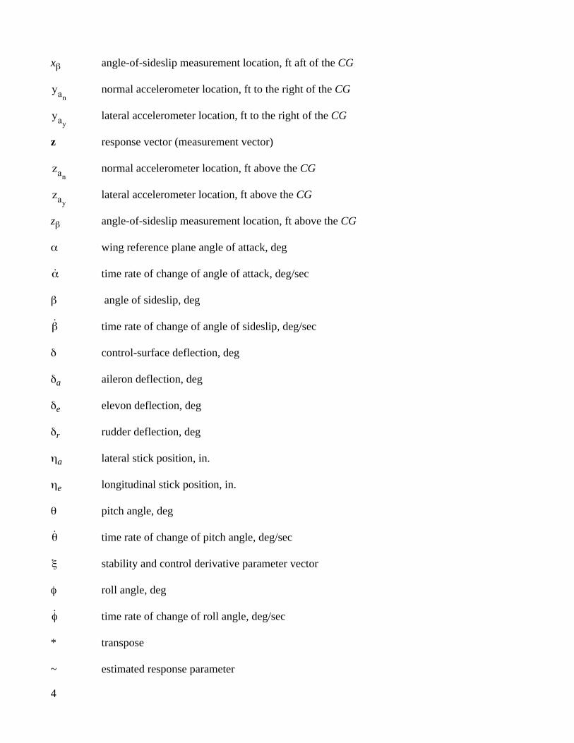
xβ angle-of-sideslip measurement location, ft aft of the CG

normal accelerometer location, ft to the right of the CG

lateral accelerometer location, ft to the right of the CG

z response vector (measurement vector)

normal accelerometer location, ft above the CG

lateral accelerometer location, ft above the CG

zβ angle-of-sideslip measurement location, ft above the CG

α wing reference plane angle of attack, deg

time rate of change of angle of attack, deg/sec

β angle of sideslip, deg

time rate of change of angle of sideslip, deg/sec

δ control-surface deflection, deg

δa aileron deflection, deg

δe elevon deflection, deg

δr rudder deflection, deg

ηa lateral stick position, in.

ηe longitudinal stick position, in.

θ pitch angle, deg

time rate of change of pitch angle, deg/sec

stability and control derivative parameter vector

φ roll angle, deg

time rate of change of roll angle, deg/sec

* transpose

~ estimated response parameter

yan

yay

zan

zay

α

β

θ

ξ

φ

5

INTRODUCTION

A Mach 3.2–capable SR-71 airplane has completed a series of flight tests at the NASA Dryden FlightResearch Center (Edwards, California). The series was performed to determine stability and controlcharacteristics of the baseline configuration (fig. 1) and two configurations with experiments mounted ontop of the fuselage. NASA Dryden previously modified the internal structure of one of its SR-71 aircraftto accommodate experiments weighing a maximum of 14,500 lb for high-speed flight research of newand unique concepts. The Linear Aerospike SR-71 Experiment (LASRE) is one example of such flightresearch (ref. 1) and consisted of an approximately 14,140-lb payload weight that was mounted to theSR-71 upper fuselage (fig. 2). The LASRE configuration obtained flight data at speeds to a maximum ofMach 1.75.

After the termination of the LASRE program, a four-flight test bed configuration flight program(ref. 2) was conducted to a maximum speed of Mach 3.0. The test bed configuration consists of theLASRE pod without the half-span lifting-body model (fig. 3). Because of the large size of the LASREand test bed configurations, an incremental stability and control flight envelope expansion becamenecessary to ensure safe flying characteristics. The envelope expansion includes pilot-input doubletmaneuvers for parameter identification (PID) of stability and control derivatives at increasing Machnumbers. Both pitch doublets and yaw-roll doublets have been performed at each Mach numbercondition. Data also have been obtained at low and high equivalent airspeeds to determine the effect ofaircraft flexibility on the stability and control derivatives. A maximum-likelihood output-error program(ref. 3) has been used postflight to estimate stability and control derivatives from the flight data. Thisreport presents flight-determined stability and control results for the SR-71 baseline, LASRE, and testbed configurations. Stability and control derivative predictions from the SR-71 aerodynamic model(ref. 4) also are presented for the baseline configuration.

VEHICLE DESCRIPTION

An SR-71A airplane (Lockheed Martin Corporation, Palmdale, California) is used as the carriervehicle for the LASRE and test bed configurations. Stability and control data have been obtained for thebaseline, LASRE, and test bed configurations that are described in this section. Because the SR-71aircraft is fairly flexible, aeroelastic effects on the stability and control derivatives also have beenobtained. Control surfaces are not modified for the LASRE and test bed configurations.

Baseline Configuration

The SR-71A aircraft is a two-place, twin-engine aircraft capable of cruising at speeds to a maximumof Mach 3.2 and altitudes to a maximum of 85,000 ft. The aircraft is powered by two 34,000-lbfthrust-class J58 (Pratt & Whitney, West Palm Beach, Florida) afterburning turbojet engines.Approximately 5 percent of thrust enhancement is obtained on both engines by increasing the turbineexhaust gas temperature and rotor speed (ref. 2). The engine is aligned with the wing reference plane,which has a 1.2-deg nosedown incidence compared to the fuselage centerline reference plane. The angle

6

of attack used herein is referenced to the wing reference plane. The engine inlet is canted slightly downand inward to obtain low local flow angles.

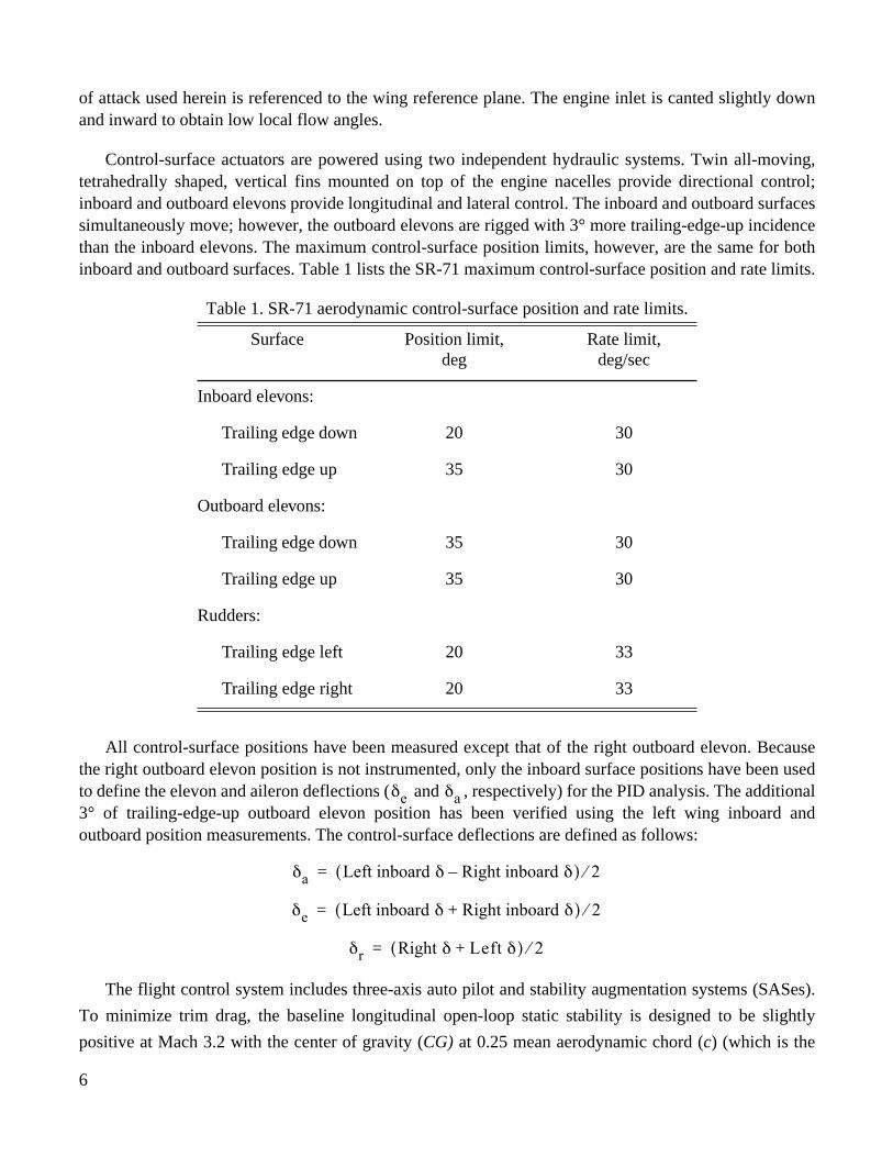
Control-surface actuators are powered using two independent hydraulic systems. Twin all-moving,tetrahedrally shaped, vertical fins mounted on top of the engine nacelles provide directional control;inboard and outboard elevons provide longitudinal and lateral control. The inboard and outboard surfacessimultaneously move; however, the outboard elevons are rigged with 3° more trailing-edge-up incidencethan the inboard elevons. The maximum control-surface position limits, however, are the same for bothinboard and outboard surfaces. Table 1 lists the SR-71 maximum control-surface position and rate limits.

All control-surface positions have been measured except that of the right outboard elevon. Becausethe right outboard elevon position is not instrumented, only the inboard surface positions have been usedto define the elevon and aileron deflections ( and , respectively) for the PID analysis. The additional3° of trailing-edge-up outboard elevon position has been verified using the left wing inboard andoutboard position measurements. The control-surface deflections are defined as follows:

The flight control system includes three-axis auto pilot and stability augmentation systems (SASes).

To minimize trim drag, the baseline longitudinal open-loop static stability is designed to be slightly

positive at Mach 3.2 with the center of gravity (CG) at 0.25 mean aerodynamic chord (c) (which is the

Table 1. SR-71 aerodynamic control-surface position and rate limits.

Surface Position limit,deg

Rate limit,deg/sec

Inboard elevons:

Trailing edge down 20 30

Trailing edge up 35 30

Outboard elevons:

Trailing edge down 35 30

Trailing edge up 35 30

Rudders:

Trailing edge left 20 33

Trailing edge right 20 33

δe δa

δa Left inboard δ Right inboard δ–( ) 2⁄=

δe Left inboard δ Right inboard δ+( ) 2⁄=

δr Right δ Left δ+( ) 2⁄=

7

operational aft CG limit). A redundant pitch SAS is used to provide good closed-loop handling qualities

at all Mach numbers. The pitch SAS uses high-passed pitch rate to augment damping and lagged pitch

rate to slightly augment stability (ref. 5). The SR-71 baseline configuration is also designed to have a

minimum, but still positive, derivative of yawing moment due to sideslip at Mach 3.2. A yaw SAS

is required to provide acceptable handling qualities at high Mach numbers and to prevent extreme

sideslip transients caused by potential inlet “unstarts.” The yaw SAS uses yaw-rate feedback for damping

and uses lateral acceleration feedback to augment stability. The effective closed-loop directional stability

provided by the yaw SAS can be computed using the following equation:

(1)

A roll SAS is used to provide roll damping through roll-rate feedback.

The empty weight of the SR-71 baseline configuration is approximately 60,700 lb. The SR-71 aircrafthas a maximum fuel capacity of 80,000 lb. For these baseline configuration tests, fuel loads of amaximum of 62,000 lb were used.

Linear Aerospike SR-71 Experiment Configuration

The LASRE configuration was developed to obtain in-flight performance data on an aerospike rocketengine. The LASRE components mounted to the top of the SR-71 airplane are referred to as the “canoe,”“kayak,” “reflection plane,” and “model” (fig. 4). Collectively, these structural components are referredto as the LASRE “pod.” The canoe was installed on the SR-71 fuselage and was designed to contain thegaseous hydrogen fuel and liquid water needed for cooling. The kayak, located beneath the reflectionplane and on top of the canoe, set the model incidence angle to 2° nosedown to align the lower part of themodel with the expected local flow over the top of the SR-71 airplane. The reflection plane was mountedon top of the kayak to help promote uniform flow in the region of the model. The model was designed toapproximate a half-span lifting body with a 70-deg swept cylinder leading edge and spherical nose.Liquid oxygen and igniter materials required to operate the rocket engine were stored in the model. Themodel was vertically mounted so that the angle of sideslip of the SR-71 airplane imparted angle of attackon the model.

With a full load of expendables, the pod weighed approximately 14,140 lb. The SR-71 fueldistribution system was adjusted to accommodate a maximum of 67,000 lb of fuel for the LASRE flights.This adjustment was made to prevent overloading the vehicle when carrying the added weight of theLASRE pod. However, actual fuel loads of a maximum of only 62,000 lb were used during the LASREflight tests. To compensate for CG shifts caused by the pod weight, 5000 lb of available fuel in theforward tank was considered unusable during the flight.

The high transonic drag of the LASRE configuration showcased the ability of the SR-71 airplane toachieve stabilized data at speeds approximating Mach 1.0. Apart from the main purpose of this report,this unique capability of the SR-71 airplane to sustain nearly Mach-1 test conditions deserves emphasis.The SR-71 physical attributes (inertia, fineness ratio, control systems, and the relative characteristics ofthe transonic drag and propulsive forces) all combine to provide a unique platform for exposing

Cnβ

Closed-loop CnβOpen-loop Cnβ

30Cnδr

qSw------CYβ

+=

8

experimental shapes to selected stabilized transonic flow conditions in a real flight environment. Theseconditions can be maintained for several minutes; and because of the relatively large size of the aircraft,the candidate models can be of a respectable scale and can include significant detail.

Figure 5 shows a time history of a nearly level–altitude acceleration from Mach 0.9 to Mach 1.1. Thisfigure shows the fairly smooth transition from subsonic to supersonic flight. Much of the accelerationwas achieved using full afterburner thrust. If desired, the pilot could stabilize at any transonic speed usingthrottle control (with the exception of stabilizing at free-stream Mach numbers between Mach 1.010 andMach 1.025, which is where the airdata Mach jump occurs). This capability makes the SR-71 airplane aunique and versatile transonic research facility that is currently available to the flight test community.This research capability of the SR-71 airplane represents a valuable complement to its well-knowncapability for flight research at high supersonic speeds to a maximum of Mach 3.2.

Test Bed Configuration

Four flights were flown with the model removed from the LASRE pod. This configuration becameknown as the test bed configuration because it can accommodate new model shapes for flight testing.The weight of the remaining canoe, kayak, and reflection plane is approximately 9400 lb. Fuel loads of amaximum of 66,000 lb were used for these tests.

The test bed configuration also demonstrated its excellent capability for transonic flight research.Figure 6 shows a time history of a nearly level–altitude acceleration from Mach 0.9 to Mach 1.1. As infigure 5, a smooth transition from subsonic to supersonic flight is seen. The angle-of-attack time historyshows two longitudinal PID doublets performed during the acceleration. Throttle control can be used tostabilize at any transonic speed (except at the airdata Mach jump).

Mass Properties

Accurate estimates of weight, CG, and mass moments of inertia were required for each PIDmaneuver. Each fuel tank is instrumented to obtain fuel quantity. The total weight is simply the sum ofthe zero-fuel weight and the total fuel weight recorded by the six tank sensors. Because of the symmetryof the left and right sides of the aircraft, only the rolling, pitching, and yawing moment and cross productof inertias (Ix, Iy, Iz, and Ixz, respectively) were required. Table 2 shows a summary of zero-fuel weight,zero-fuel weight CG, and zero-fuel inertias for the three flight configurations. Figure 7 shows thebody-axis mass moments of inertia for the baseline configuration (using the standard fuel burn schedule)as a function of total vehicle weight.

Fuel quantity measurements from the six fuselage fuel tanks are used to compute the CG. Each fueltank CG is a function of both measured fuel quantity and aircraft pitch attitude. For the LASRE and testbed configurations, pod component CGs are also used to obtain the total configuration CG. Flight datawere obtained at CGs ranging from 0.173 c to 0.258 c. Individual fuel quantity measurements and podcomponent mass distribution information are used to compute the inertias at each test condition.

9

METHODS OF ANALYSIS

This section describes the formulation of the output-error parameter estimation technique used toanalyze the flight data. The nonlinear equations of motion used in the analysis also are defined.

Parameter Identification Formulation

The primary objective of this research is to estimate from flight test the stability and controlderivatives for each of these SR-71 configurations. The actual vehicle system is described by a vector setof dynamic equations of motion that are defined in the next section. The form of these equations isassumed to be known, but the time-invariant aerodynamic stability and control parameters in theseequations are unknown. The PID flight test maneuvers are designed to record the response of the aircraftsystem to measured control inputs. The parameter estimation program known as pEst (ref. 3) is used inpostflight analysis to adjust the unknown parameter values in the model until the estimated aircraftresponse agrees with the measured response.

The pEst program defines a cost function that can be used to quantitatively measure the agreementbetween the computed response and the actual measured response of the model. The pEst programsearches for the unknown parameter values to minimize the cost function.

Table 2. Zero-fuel weight, CG, and mass moment of inertia information for the three SR-71configurations.

SR-71 zero-fuel weight CG

Configuration Flight numbers

SR-71 zero-fuelweight, lb

Fuselage station, in.

Mean aerodynamicchord, percent

SR-71 zero-fuel inertias,slug-ft2

Baseline 37–44 60,728 877.9 20.1

Ix = 220,660Iy = 954,850

Iz = 1,172,039Ixz = 19,200

LASRE 45–48 74,032 911.0 27.4

Ix = 230,880Iy = 1,035,140Iz = 1,252,330

Ixz = 44,640

LASRE 49–51 75,349 910.6 27.3

Ix = 230,880Iy = 1,035,520Iz = 1,252,710

Ixz = 44,710

Test bed 52–55 70,158 892.3 23.3

Ix = 224,670Iy = 992,280

Iz = 1,209,470Ixz = 28,390

10

To obtain the cost function, the pEst program must solve a vector set of time-varying ordinarydifferential equations of motion. The equations of motion are separated into a continuous-time stateequation and a discrete-time response equation:

(2)

(3)

where F is the state derivative function, G is the response function, x is the state vector, is the timederivative of the state vector, z is the response or measurement vector, u is the measured control inputvector, is the stability and control derivative parameter vector, and t is time. For this application ofstability and control derivative estimation, state noise is assumed to not exist.

The output-error cost function, J(ξ), used by the pEst program is as follows:

(4)

where nt is the number of time history points used, nz is the number of response variables, is theestimated response vector, and W is the response weighting matrix. The superscript * denotes transpose.

For each possible estimate of the unknown parameters, a probability that the aircraft response timehistories attain values approximating the observed values can be defined. The maximum-likelihoodestimates are defined as those estimates that maximize this probability. Minimizing the cost functiongives the maximum-likelihood estimate of the stability and control parameters.

Figure 8 shows the maximum-likelihood parameter estimation process. The measured response iscompared with the estimated response, and the difference between these, called the response error, isincluded in the cost function. The minimization algorithm is used to find the coefficient values thatminimize the cost function. Each iteration of this algorithm provides a new estimate of the unknowncoefficients on the basis of the response error. These new estimates are then used to update values of thecoefficients of the mathematical model, providing a new estimated response and, therefore, a newresponse error. Updating the mathematical model iteratively continues until a convergence criterion issatisfied (in this case, the ratio of the change in total cost to the total cost, ∆J(ξ)/J(ξ), must be less than0.000001). The estimates resulting from this procedure are the maximum-likelihood estimates.

The estimator also provides a measure of the reliability of each estimate based on the informationobtained from each dynamic maneuver. This measure of reliability is called the Cramér-Rao bound(ref. 6). The Cramér-Rao bound is a measure of relative, not absolute, accuracy. A large Cramér-Raobound indicates poor information content in the maneuver for the derivative estimate.

Equations of Motion

The aircraft equations of motion used in the PID analysis are derived from a general system of ninecoupled, nonlinear differential equations that describe the aircraft motion (ref. 4). These equations

x t( ) F x t( ) u t( ), ξ[ , ]=

z ti( ) G x ti( ) u ti( ), ξ[ , ]=

x

ξ

J ξ( ) 12nznt------------- z ti( ) z ti( )–[ ]

*W z ti( ) z ti( )–[ ]

i 1=

nt

∑=

z

11

assume a rigid vehicle and a flat, nonrotating Earth. The time rate of change of mass and inertia isassumed negligible. The SR-71 configurations studied herein, like most aircraft, are basically symmetricabout the vertical-centerline plane. This symmetry is used, along with small angle approximations, toseparate the equations of motion into two largely independent sets describing the longitudinal andlateral-directional motions of the aircraft. The equations of motion are written in body axes referenced tothe CG and include both state and response equations. The applicable equations of motion are as followsfor the longitudinal and lateral-directional axes:

Longitudinal state equations:

(5)

(6)

(7)

Longitudinal response equations:

(8)

(9)

(10)

(11)

where and are estimates of instrumentation biases and R is a conversion factor betweendegrees and radians.

Lateral-directional state equations:

(12)

(13)

(14)

(15)

α qSRmV βcos---------------------CN α q β p α r αsin+cos( ) gR

V βcos---------------- φ θ α θ αsinsin+coscoscos( )+tan–+cos–=

qIy qScCmR rp Iz Ix–( ) r2

p2

–( )Ixz+[ ] R⁄+=

θ q φcos r φsin–=

α α xαqV----+=

q q qbias+=

θ θ=

an˜ qS

mg--------CN

1gR------- xan

q yanp+– 1

gR2

----------zanq

2p

2+( )– anbias

+=

qbias anbias

β qSRmV-----------CY p αsin r αcos– gR

V------- φ θ βcoscossin β θ φcos αsincos θ αcossin–( )sin–[ ]+ +=

pIx rIxz– qSbClR qr Iy Iz–( ) pqIxz+[ ] R⁄+=

rIz pIxz– qSbCnR pq Ix Iy–( ) qrIxz–[ ]+ R⁄=

φ p q θtan φsin r θtan φcos+ +=

12

Lateral-directional response equations:

(16)

(17)

(18)

(19)

(20)

where , , and are estimates of instrumentation biases.

Equations (5)–(20) contain locally linear approximations of the aerodynamic coefficients. Thelongitudinal aerodynamic coefficients are expanded as follows:

(21)

(22)

The coefficients are based on a reference area of 1605 ft2 and a mean aerodynamic chord of 37.7 ft.The coefficient with the subscript “b” is a linear extrapolation of the angle-of-attack derivative fromthe average angle of attack of the maneuver to 0° angle of attack (ref. 6). Axial force coefficients arenot used in this analysis because the engine performance model is not well known, but this is not aconcern because the axial force derivatives do not significantly affect flying qualities. All thelongitudinal derivatives in equations (21)–(22) are estimated in the analysis.

The lateral-directional aerodynamic coefficients are expanded as follows:

(23)

(24)

(25)

β β zβpV---- xβ

rV----– βbias+ +=

p p pbias+=

r r rbias+=

φ φ=

ay˜ qS

mg--------CY

1gR------- x– ay

r zayp+ 1

gR2

----------yayp

2r2

+( )–+=

βbias pbias rbias

CN CNbCNα

α c2VR------------CNq

q CNδe

δe+ + +=

Cm CmbCmα

α c2VR------------Cmq

q Cmδe

δe+ + +=

CY CYbCYβ

β b2VR------------ CYp

p CYrr+( ) CYδa

δa CYδr

δr+ + + +=

Cl ClbClβ

β b2VR------------ Clp

p Clrr+( ) Clδa

δa Clδr

δr+ + + +=

Cn CnbCnβ

β b2VR------------ Cnp

p Cnrr+( ) Cnδa

δa Cnδr

δr+ + + +=

13

The reference span, b, is 56.7 ft. The coefficient with the subscript “b” is a linear extrapolation of theangle-of-sideslip derivative from the average angle of sideslip of the maneuver to 0° angle of sideslip. Allthe lateral-directional derivatives in equations (23)–(25) were estimated in the analysis.

INSTRUMENTATION AND DATA ACQUISITION

The SR-71 airplane is equipped with a complete set of research airdata and inertial instrumentation.Free-stream pitot-static airdata are obtained from a calibrated noseboom. Angle-of-attack and -sideslipdata are obtained from a four-hole hemispherical probe doglegged to the noseboom. The angle of attackis referenced to the wing reference plane, which is 1.2-deg nosedown in incidence compared to thefuselage centerline reference plane. Angle-of-attack and -sideslip measurements are lagged on the orderof 0.2 to 0.4 sec because of the pneumatic plumbing. These lags are accounted for by time skews in thedata analysis. Pitch and roll attitude data are obtained from the SR-71 inertial navigation system.Three-axis angular rate and linear accelerations are measured using strapdown sensors installed atfuselage station (FS) 683.0, butt line (BL) 32.5, and water line (WL) 86.2.

Signal conditioning on the angular rate and acceleration measurements includes a first-order passiveantialiasing filter with a 40-Hz rolloff frequency. This filter imparts a 45-deg phase lag that is equivalentto a 3-msec time lag. This time lag is less than the sample time interval of 5 msec. Although measured atsample rates that are higher, the flight data are thinned to 20 samples/sec for the PID analysis. Angles ofattack and sideslip and linear accelerations are corrected in the mathematical model of the pEst programto the CG using angular rate measurements and sensor position information. Vehicle weight andlongitudinal CG location are obtained using fuel tank measurements. Laterally and vertically, the CG isassumed to be located at BL 0 and WL 100, respectively. All control-surface positions are measured withthe exception of the right outboard elevon. For the PID analysis, only the inboard surface positions areused to define the elevon and aileron deflections.

In the PID analysis, angle of attack and normal acceleration are the primary aircraft responses used toobtain normal force coefficient estimations. Similarly, angle of sideslip and lateral acceleration are usedto obtain side force coefficient estimates. Because of uncertainties in the calibration and pneumatic lagsassociated with the flow angle measurements, larger weights are assigned to the acceleration responsemeasurements in the PID analysis than to the flow angle response measurements. The response weightsare constant for all configurations tested, with the exception of a few cases where temporaryinstrumentation problems existed.

FLIGHT TEST APPROACH

The objective of this research is to obtain baseline SR-71 stability and control derivatives from PIDflight data. When the baseline derivatives are known, the aerodynamic effects of the LASRE and test bedconfigurations can then be obtained from further PID flight testing. An “envelope expansion” approachhas been used to safely “clear” the configuration to the desired maximum Mach number. The envelopewas expanded by incrementally increasing Mach number and performing PID doublet maneuvers. Thepilots evaluated the airplane handling qualities in real time, and the PID maneuvers were analyzedpostflight using the pEst program to obtain stability and control derivative estimates. Therefore, multipleflights were required to clear the envelope for safe operations.

14

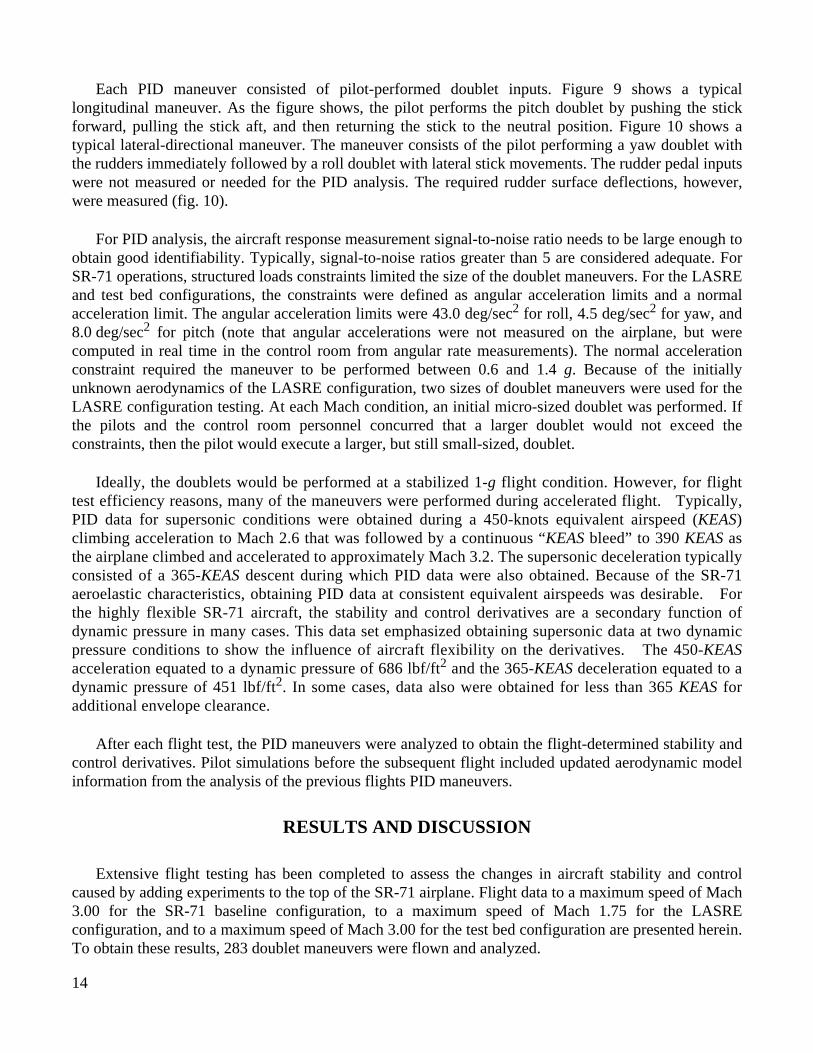
Each PID maneuver consisted of pilot-performed doublet inputs. Figure 9 shows a typicallongitudinal maneuver. As the figure shows, the pilot performs the pitch doublet by pushing the stickforward, pulling the stick aft, and then returning the stick to the neutral position. Figure 10 shows atypical lateral-directional maneuver. The maneuver consists of the pilot performing a yaw doublet withthe rudders immediately followed by a roll doublet with lateral stick movements. The rudder pedal inputswere not measured or needed for the PID analysis. The required rudder surface deflections, however,were measured (fig. 10).

For PID analysis, the aircraft response measurement signal-to-noise ratio needs to be large enough toobtain good identifiability. Typically, signal-to-noise ratios greater than 5 are considered adequate. ForSR-71 operations, structured loads constraints limited the size of the doublet maneuvers. For the LASREand test bed configurations, the constraints were defined as angular acceleration limits and a normalacceleration limit. The angular acceleration limits were 43.0 deg/sec2 for roll, 4.5 deg/sec2 for yaw, and8.0 deg/sec2 for pitch (note that angular accelerations were not measured on the airplane, but werecomputed in real time in the control room from angular rate measurements). The normal accelerationconstraint required the maneuver to be performed between 0.6 and 1.4 g. Because of the initiallyunknown aerodynamics of the LASRE configuration, two sizes of doublet maneuvers were used for theLASRE configuration testing. At each Mach condition, an initial micro-sized doublet was performed. Ifthe pilots and the control room personnel concurred that a larger doublet would not exceed theconstraints, then the pilot would execute a larger, but still small-sized, doublet.

Ideally, the doublets would be performed at a stabilized 1-g flight condition. However, for flighttest efficiency reasons, many of the maneuvers were performed during accelerated flight. Typically,PID data for supersonic conditions were obtained during a 450-knots equivalent airspeed (KEAS)climbing acceleration to Mach 2.6 that was followed by a continuous “KEAS bleed” to 390 KEAS asthe airplane climbed and accelerated to approximately Mach 3.2. The supersonic deceleration typicallyconsisted of a 365-KEAS descent during which PID data were also obtained. Because of the SR-71aeroelastic characteristics, obtaining PID data at consistent equivalent airspeeds was desirable. Forthe highly flexible SR-71 aircraft, the stability and control derivatives are a secondary function ofdynamic pressure in many cases. This data set emphasized obtaining supersonic data at two dynamicpressure conditions to show the influence of aircraft flexibility on the derivatives. The 450-KEASacceleration equated to a dynamic pressure of 686 lbf/ft2 and the 365-KEAS deceleration equated to adynamic pressure of 451 lbf/ft2. In some cases, data also were obtained for less than 365 KEAS foradditional envelope clearance.

After each flight test, the PID maneuvers were analyzed to obtain the flight-determined stability andcontrol derivatives. Pilot simulations before the subsequent flight included updated aerodynamic modelinformation from the analysis of the previous flights PID maneuvers.

RESULTS AND DISCUSSION

Extensive flight testing has been completed to assess the changes in aircraft stability and controlcaused by adding experiments to the top of the SR-71 airplane. Flight data to a maximum speed of Mach3.00 for the SR-71 baseline configuration, to a maximum speed of Mach 1.75 for the LASREconfiguration, and to a maximum speed of Mach 3.00 for the test bed configuration are presented herein.To obtain these results, 283 doublet maneuvers were flown and analyzed.

15

Simulation predictions of the baseline derivatives have been compared with flight data. Thesimulation predictions come from a workstation-based batch simulation. The aerodynamic modelincorporated into the simulator came from the SR-71 baseline aerodynamic model (ref. 4). Predictedstability and control derivatives were obtained by linearizing the aerodynamic model at the flight testMach number, altitude, and mass property conditions. Simulation predictions will be plotted only tocompare with the baseline configuration flight results. Predicted increments to the stability and controlderivatives caused by the LASRE pod installation were obtained in wind-tunnel tests and published inreference 7. No wind-tunnel predictions, however, were obtained for the test bed configuration.

The PID analysis was used to estimate the open-loop stability and control derivatives from pilot-inputdoublet maneuvers. Stability augmentation systems were used at all times in all axes to increase theclosed-loop stability and damping. With the SASes remaining on, autopilots were turned off for the axesof interest during the PID maneuvers. Some of the initial flight test results for the test bed configurationhave been published in reference 2 and for the baseline and LASRE configurations in reference 8.

For the LASRE configuration, both micro-sized and larger, but still small-sized, doublets wereperformed. In many cases, the PID analysis shows good fits of the measured and estimated responseparameters for the micro-sized doublets. However, the Cramér-Rao bounds were usually larger for themicro-sized doublets than for the small-sized doublets because of smaller signal-to-noise ratios; and theparameter estimate sometimes differed from multiple estimates using the micro-sized doublet. Therefore,only small-sized doublet results are presented in this report.

Figures 11–13 show the flight envelope available for this testing and the Mach number and altitudeflight conditions used for the baseline, LASRE, and test bed configurations, respectively. The flightconditions referred to as “low-KEAS” test points are shown in the shaded regions of figures 11–13. Theremaining test points are considered “high-KEAS” test points. The distinction between low-KEAS andhigh-KEAS test points is important because, in some cases, aircraft flexibility affected the stability andcontrol derivatives. The flexibility effects were included in the baseline aerodynamic model (ref. 2).

Flight data were obtained at CG values ranging between 0.173 and 0.258 c. All moment derivativeswere estimated about the flight CG using the pEst program. For presentation in this report, the pitchingand yawing moment derivatives were corrected to the moment reference using flight-estimated normaland side force derivatives, respectively (ref. 9). The moment reference is located at 0.25 c (FS 900).

Scatter in derivative estimates could be caused by maneuvers being performed at different weights,angles of attack, trim elevon positions, and bank angles. Slight variations in maneuver sizes, flexibilityeffects, and not accounting for engine gyroscopic effects (which are assumed negligible) could also resultin data scatter. As stated previously, the Cramér-Rao bounds (ref. 6) are used as a measure of relative,but not absolute, accuracy. Large Cramér-Rao bounds indicate poor information content in the maneuverfor the derivative estimate. The Cramér-Rao bounds plotted in this report have been multiplied by afactor of five to increase clarity.

16

Longitudinal Derivatives

Longitudinal stability and control derivatives were determined independently from lateral-directionalderivatives. This section presents results from the SR-71 baseline, LASRE, and test bed configurationsobtained using longitudinal PID pitch doublet maneuvers. A comparison of the stability and controlderivatives obtained from the three configurations also will be shown.

Baseline Configuration

Figure 14 shows time histories from typical subsonic, transonic, and supersonic test points. Thesetime histories include pilot stick inputs, elevon control-surface positions, and aircraft responses for angleof attack, pitch rate, pitch attitude, and normal acceleration. For the response parameters, the solid linesrepresent measured aircraft responses and the dashed lines represent the responses obtained byintegrating the equations of motion using the pEst estimates of the stability and control derivatives. Asfigure 14 shows, the angle-of-attack response shows the worst fit between measured and pEst-estimatedresponses. This result is not surprising because in the pEst program, the angle-of-attack measurement isweighted less than the normal acceleration measurement because of high confidence in the normalacceleration measurement as explained in the “Instrumentation and Data Acquisition” section. Figures15–18 show the baseline longitudinal stability and control derivatives.

Figure 15 shows coefficient of normal force and pitching moment bias ( and ) estimates.The circle symbols represent high-KEAS test points and the cross symbols represent low-KEAS testpoints. The solid and dashed lines are fairings of the high- and low-KEAS results, respectively. Thesefairings are based on the authors’ interpretation of the trends in the flight estimates. The vertical bars onthe plots represent the scaled Cramér-Rao bounds. The do not show significant differences causedby flexibility. The show reduced values at supersonic speeds for the low-KEAS test points,especially at approximately Mach 1.8. Note that these bias values are not the traditional normal force andpitching moment coefficients at 0° angle of attack with no surface deflections. The parameter estimationprogram, pEst, uses a maximum-likelihood technique to obtain a linear fit of the data around the trimpoint. The bias is simply the extrapolation of the linear fit to 0° angle of attack. For these test points, thetrimmed wing reference plane angle of attack varied between 2.5° and 6°. The baseline aerodynamicmodel (ref. 4) contains a reasonably linear normal force coefficient over this angle-of-attack range, butthe pitching moment coefficient typically was nonlinear. Also, reference 4 shows that the nonlinear effectof aircraft flexibility on pitching moment becomes increasingly significant at supersonic Mach numbers,which is consistent with the observed change in pitching moment coefficient bias estimates at supersonicspeeds caused by aircraft flexibility.

Figure 16 shows the angle-of-attack derivatives. The thin solid lines are the simulation-predicted

values for the high-KEAS test points, and the thin dashed lines are the simulation-predicted values for the

low-KEAS test points. The flight data show reduced values for derivatives of normal force due to angle of

attack, , compared to the simulation values. The flight data also show the simulation-predicted

flexibility effects (fig. 16(a)).

CNbCmb

CNbCmb

CNα

17

Figure 16(b) shows the derivative of pitching moment due to angle of attack, . The flight data

show slightly reduced static stability (that is, less negative) compared with the simulator values, and the

flexibility effects at supersonic Mach numbers are not as pronounced in the flight data. Note that is

computed about the 0.25-c moment reference point. The positive values at subsonic Mach numbers do

not indicate that the airplane was ever flown with negative static margins. For those test points, the CG

was significantly forward of the 0.25-c reference location. As figure 16(b) also shows, the static stability

tends toward zero as Mach number is increased. This tendency was expected because the SR-71 aircraft

is designed to have minimum open-loop static stability at the design cruise Mach number of 3.2 to reduce

trim drag (ref. 4). The design Mach 3.2 cruise CG location for acceptable stability and trim drag is 0.25 c.

Figure 17 shows the dynamic derivatives. The baseline aerodynamic model (ref. 4) assumes a zero

value for the derivative of normal force due to nondimensional pitch rate, . The flight data show

generally decreases as Mach number increases (figure 17(a)). The derivative of pitching moment

due to nondimensional pitch rate, , measured in flight was larger (that is, a more negative derivative)

than predicted, with the exception of the data recorded at Mach 2.5 (fig. 17(b)). The reason for the

variation in the derivative estimates at Mach 2.5 is suspected to be that the two test points with positive

values were flown at an altitude of 65,000 ft and the two test points with negative values were flown at an

altitude of 60,000 ft. Although the simulator predicted no difference in the for these two conditions,

open-loop damping is known to decrease as altitude increases (ref. 4). Open-loop damping is also

expected to be reduced as the Mach number increases toward the Mach-3.2 design condition. The test

point at Mach 3.0 was flown at an altitude of 80,000 ft and showed a negative value that causes the

values recorded at Mach 2.5 and an altitude of 65,000 ft to be suspect (although only one test point was

obtained at Mach 3.0).

Figure 18 shows the elevator control derivatives. The flight-determined normal force derivative

estimates are less than predicted (fig. 18(a)). For supersonic conditions, the flight-determined normal

force derivative estimates were almost zero. The flexibility effects predicted by the simulation are evident

in the flight data. The flight-estimated near-zero elevator contribution to normal force seemed anomalous

to the authors; however, further scrutiny of the analysis consistently confirmed the result that deflecting

the elevators had little effect on normal force. An equation-error PID technique (ref. 10) also was used to

analyze these data and shows the same result. Figure 18(b) shows the pitching moment effectiveness of

the elevator. The flight data and simulator predictions agree well and the flexibility effects are clearly

seen, especially at supersonic-condition Mach numbers where a clear distinction exists between low- and

high-KEAS test points. This aeroelastic effect was expected because control surfaces on flexible aircraft

typically become less effective as dynamic pressure increases.

Cmα

Cmα

CNq

CNq

Cmq

Cmq

Cmq

18

Linear Aerospike SR-71 Experiment Configuration

Figure 19 shows time histories from typical test points for the LASRE configuration at subsonic,transonic, and supersonic conditions. Good fits were obtained between the measured and pEst-estimatedresponses; angle-of-attack fit is the most noticeably off. The measured pitch rate (fig. 19(b)) shows a2-Hz response that is caused by the fuselage first-bending mode. Some maneuvers not shown in figure 19also show a 2-Hz response in the normal accelerometer output. The pEst implementation used in thisresearch assumes rigid body motion and was expected to identify aircraft flexibility effects that resultfrom changes in dynamic pressure. The pEst program was not expected to identify the high-frequencystructural modes because no structural equations of motion are included in the formulation. Therefore,the pEst-estimated responses are not expected to match this observed 2-Hz motion.

Figures 20–23 show the LASRE configuration longitudinal stability and control derivatives. Only afew low-KEAS test points were obtained during the LASRE program; these points were at Mach numbersapproximating 0.90, 1.20, and 1.45 (fig. 9).

Figures 20(a) and 20(b) show the and , respectively. A negative is seen across the

Mach range tested. The pitching moment coefficient bias is negative (nosedown) for subsonic conditions,

shows a large positive (noseup) value for transonic conditions, and then shows a constant positive value

for supersonic conditions. Flexibility effects are seen in the and during flight at Mach 1.45.

Figure 21 shows angle-of-attack derivatives. No clear flexibility effects are evident from the flight data.

Figure 22 shows the dynamic derivatives, and figure 23 shows the elevator effectiveness derivatives. As

with the baseline configuration, the elevators are consistently more effective at the low-KEAS test points

(fig. 23(b)).

Test Bed Configuration

Figure 24 shows time histories from typical test points for the test bed configuration at subsonic,transonic, and supersonic conditions. Good fits were obtained between the measured and pEst-estimatedresponses; angle-of-attack fit again is the most noticeably off. Figure 24(c) shows that the airplaneresponses at Mach 3.02 were very small, although the stick inputs and elevon deflections wereapproximately the same magnitude as at low-speed conditions. These small responses resulted in some ofthe high-speed derivative estimates having larger Cramér-Rao bounds (because of smaller responsemeasurement signal-to-noise ratios) than low-speed test points.

Figures 25–28 show the test bed configuration longitudinal stability and control derivatives. Figure13 shows the flight test conditions. As figure 13 shows, the majority of the low-KEAS points are at365 KEAS and the majority of the high-KEAS points are at 450 KEAS.

Figure 25 shows the and . Some flexibility effects have been identified. Figure 26 shows

the angle-of-attack derivatives. High-KEAS test points at Mach 2.10 and Mach 2.23 did show a

significantly reduced for the test bed configuration (fig. 26(b)). These results were obtained on the

second test bed flight; the results were not repeated on the third test bed flight when doublets were flown

CNbCmb

CNb

CNbCmb

CNbCmb

Cmα

19

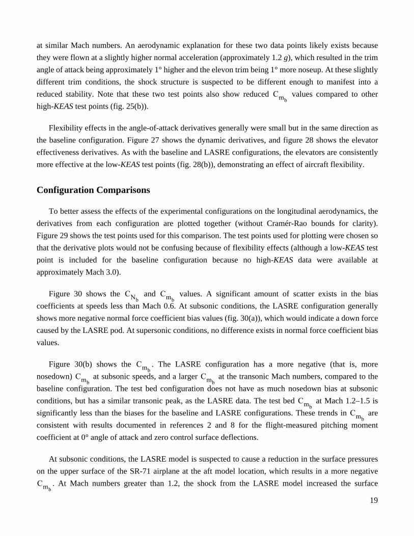
at similar Mach numbers. An aerodynamic explanation for these two data points likely exists because

they were flown at a slightly higher normal acceleration (approximately 1.2 g), which resulted in the trim

angle of attack being approximately 1° higher and the elevon trim being 1° more noseup. At these slightly

different trim conditions, the shock structure is suspected to be different enough to manifest into a

reduced stability. Note that these two test points also show reduced values compared to other

high-KEAS test points (fig. 25(b)).

Flexibility effects in the angle-of-attack derivatives generally were small but in the same direction as

the baseline configuration. Figure 27 shows the dynamic derivatives, and figure 28 shows the elevator

effectiveness derivatives. As with the baseline and LASRE configurations, the elevators are consistently

more effective at the low-KEAS test points (fig. 28(b)), demonstrating an effect of aircraft flexibility.

Configuration Comparisons

To better assess the effects of the experimental configurations on the longitudinal aerodynamics, the

derivatives from each configuration are plotted together (without Cramér-Rao bounds for clarity).

Figure 29 shows the test points used for this comparison. The test points used for plotting were chosen so

that the derivative plots would not be confusing because of flexibility effects (although a low-KEAS test

point is included for the baseline configuration because no high-KEAS data were available at

approximately Mach 3.0).

Figure 30 shows the and values. A significant amount of scatter exists in the bias

coefficients at speeds less than Mach 0.6. At subsonic conditions, the LASRE configuration generally

shows more negative normal force coefficient bias values (fig. 30(a)), which would indicate a down force

caused by the LASRE pod. At supersonic conditions, no difference exists in normal force coefficient bias

values.

Figure 30(b) shows the . The LASRE configuration has a more negative (that is, more

nosedown) at subsonic speeds, and a larger at the transonic Mach numbers, compared to the

baseline configuration. The test bed configuration does not have as much nosedown bias at subsonic

conditions, but has a similar transonic peak, as the LASRE data. The test bed at Mach 1.2–1.5 is

significantly less than the biases for the baseline and LASRE configurations. These trends in are

consistent with results documented in references 2 and 8 for the flight-measured pitching moment

coefficient at 0° angle of attack and zero control surface deflections.

At subsonic conditions, the LASRE model is suspected to cause a reduction in the surface pressures

on the upper surface of the SR-71 airplane at the aft model location, which results in a more negative

. At Mach numbers greater than 1.2, the shock from the LASRE model increased the surface

Cmb

CNbCmb

CmbCmb

Cmb

CmbCmb

Cmb

20

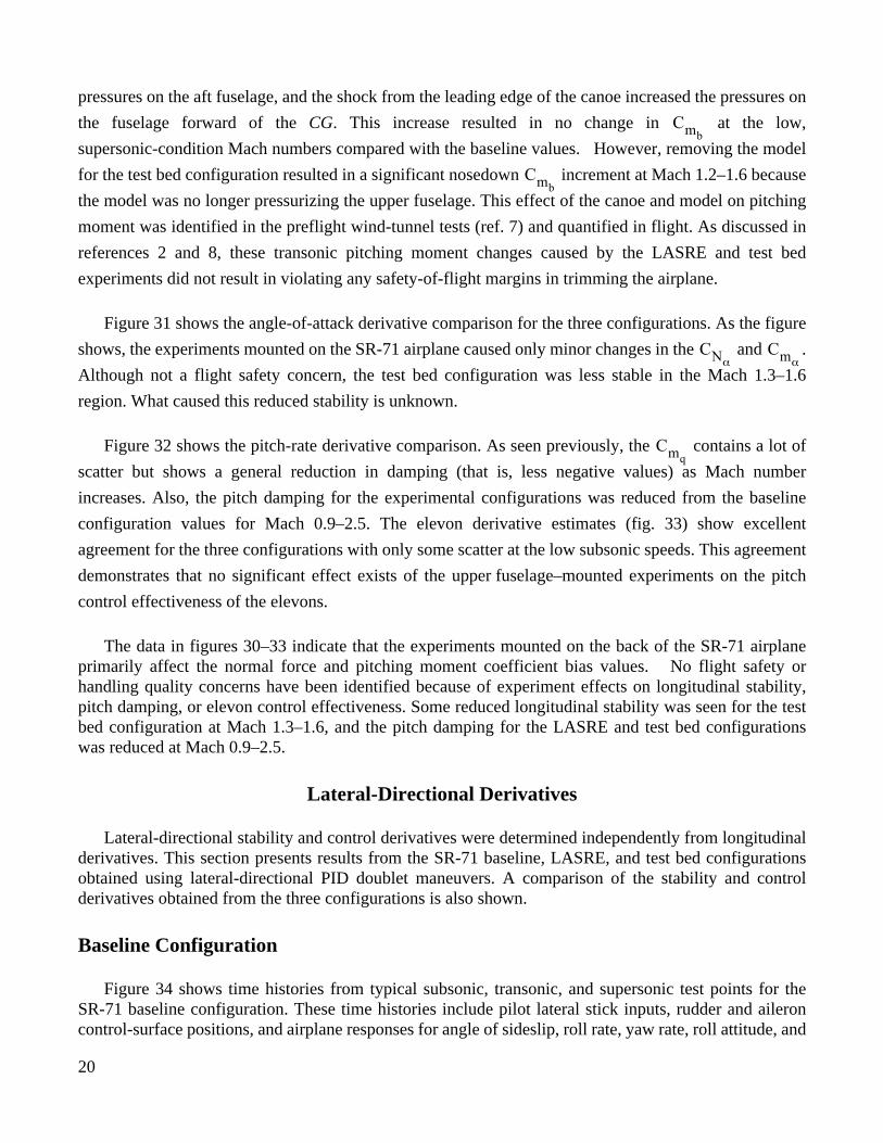
pressures on the aft fuselage, and the shock from the leading edge of the canoe increased the pressures on

the fuselage forward of the CG. This increase resulted in no change in at the low,

supersonic-condition Mach numbers compared with the baseline values. However, removing the model

for the test bed configuration resulted in a significant nosedown increment at Mach 1.2–1.6 because

the model was no longer pressurizing the upper fuselage. This effect of the canoe and model on pitching

moment was identified in the preflight wind-tunnel tests (ref. 7) and quantified in flight. As discussed in

references 2 and 8, these transonic pitching moment changes caused by the LASRE and test bed

experiments did not result in violating any safety-of-flight margins in trimming the airplane.

Figure 31 shows the angle-of-attack derivative comparison for the three configurations. As the figure

shows, the experiments mounted on the SR-71 airplane caused only minor changes in the and .

Although not a flight safety concern, the test bed configuration was less stable in the Mach 1.3–1.6

region. What caused this reduced stability is unknown.

Figure 32 shows the pitch-rate derivative comparison. As seen previously, the contains a lot of

scatter but shows a general reduction in damping (that is, less negative values) as Mach number

increases. Also, the pitch damping for the experimental configurations was reduced from the baseline

configuration values for Mach 0.9–2.5. The elevon derivative estimates (fig. 33) show excellent

agreement for the three configurations with only some scatter at the low subsonic speeds. This agreement

demonstrates that no significant effect exists of the upper fuselage–mounted experiments on the pitch

control effectiveness of the elevons.

The data in figures 30–33 indicate that the experiments mounted on the back of the SR-71 airplaneprimarily affect the normal force and pitching moment coefficient bias values. No flight safety orhandling quality concerns have been identified because of experiment effects on longitudinal stability,pitch damping, or elevon control effectiveness. Some reduced longitudinal stability was seen for the testbed configuration at Mach 1.3–1.6, and the pitch damping for the LASRE and test bed configurationswas reduced at Mach 0.9–2.5.

Lateral-Directional Derivatives

Lateral-directional stability and control derivatives were determined independently from longitudinalderivatives. This section presents results from the SR-71 baseline, LASRE, and test bed configurationsobtained using lateral-directional PID doublet maneuvers. A comparison of the stability and controlderivatives obtained from the three configurations is also shown.

Baseline Configuration

Figure 34 shows time histories from typical subsonic, transonic, and supersonic test points for theSR-71 baseline configuration. These time histories include pilot lateral stick inputs, rudder and aileroncontrol-surface positions, and airplane responses for angle of sideslip, roll rate, yaw rate, roll attitude, and

Cmb

Cmb

CNαCmα

Cmq

21

lateral acceleration. For the response parameters, the solid lines represent measured airplane responses,and the dashed lines represent the responses obtained by integrating the equations of motion using thepEst estimates of the stability and control derivatives. Good fits between the measured andpEst-estimated responses were obtained for all of the response parameters. Figures 35–40 show thelateral-directional stability and control derivatives for the baseline configuration.

Figure 35 shows the coefficients of side force, rolling moment, and yawing moment biases, ,, and . The SR-71 aircraft is basically symmetrical about the vertical-centerline plane and all

maneuvers were trimmed at almost 0° angle of sideslip. Because the PID maneuvers were done with onlysmall variations in angle of sideslip about 0° and because the aerodynamics are almost linear at thesesmall sideslip angles, the bias values were expected to be approximately zero. For the most part, the flightdata did show bias values at approximately zero (fig. 35).

Figure 36 shows the angle-of-sideslip derivatives. The estimated derivative of side force due to

sideslip, , was typically 25-percent less than predicted (figure 36(a)). The trends with Mach number

and the lack of flexibility effects agree with the simulation. The derivative of rolling moment due to

sideslip, , agrees well with predictions (figure 36(b)). The is more negative at the low-KEAS test

points compared to the high-KEAS test points, as was predicted by the simulation and as was expected

for a flexible aircraft. The estimated in flight agrees very well with predictions (fig. 36(c)), with the

only difference being an improvement in stability (that is, more positive value) at Mach 2. The SR-71

aircraft was designed to have minimum directional static stability at the design cruise speed of Mach 3.2

(ref. 4) to save tail weight and drag.

Figure 37 shows the dynamic derivatives due to roll rate. The derivative of rolling moment due to

nondimensional roll rate, , is less than predicted and shows an aeroelastic effect (figure 37(b)).

Figure 38 shows the dynamic derivatives due to yaw rate. The derivative of yawing moment due to

nondimensional yaw rate, , was higher (that is, a more negative value) than predicted for Mach

numbers less than 2.5 (fig. 38(c)). As Mach number increases beyond 2.5, the flight data suggests

negative open-loop yaw damping (that is, positive values of ). Reduced yaw damping is seen for

some of the low-KEAS test points at supersonic conditions. The combination of low aerodynamic yaw

damping and low directional stability (fig. 36(c)) at high-supersonic conditions resulted in the

requirement for a yaw-axis SAS for adequate closed-loop handling qualities (refs. 4 and 5).

Figure 39 shows the rudder derivatives. Generally, slightly lower side force and higher rollingmoment effectiveness values were seen in flight compared to predictions. The flight data agree well withthe predicted yawing moment effectiveness values of the rudders, with the exception of lowerflight-determined values at subsonic conditions.

Figure 40 shows the aileron derivatives. The simulation uses zero for the derivative of side force dueto aileron. The flight data estimated a small number slightly greater than zero (fig. 40(a)). The flight dataagree well with the predicted derivative of rolling moment due to aileron, , except at approximately

CYbClb

Cnb

CYβ

ClβClβ

Cnβ

Clp

Cnr

Cnr

Clδa

22

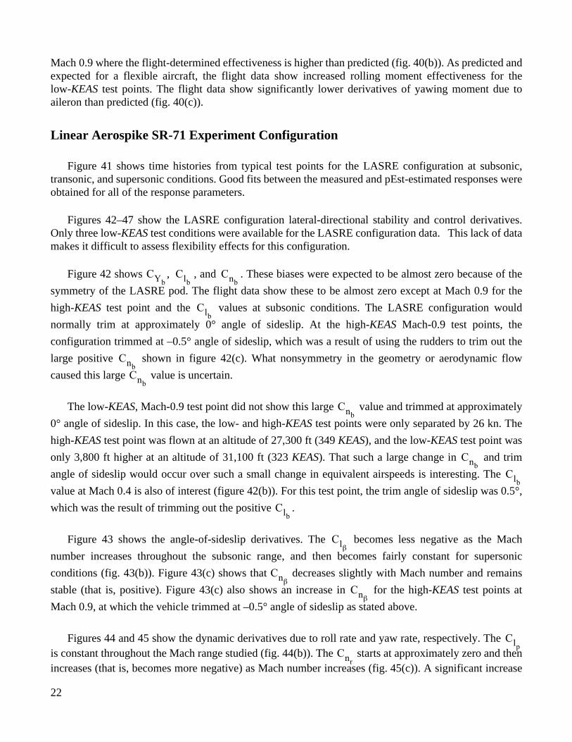
Mach 0.9 where the flight-determined effectiveness is higher than predicted (fig. 40(b)). As predicted andexpected for a flexible aircraft, the flight data show increased rolling moment effectiveness for thelow-KEAS test points. The flight data show significantly lower derivatives of yawing moment due toaileron than predicted (fig. 40(c)).

Linear Aerospike SR-71 Experiment Configuration

Figure 41 shows time histories from typical test points for the LASRE configuration at subsonic,transonic, and supersonic conditions. Good fits between the measured and pEst-estimated responses wereobtained for all of the response parameters.

Figures 42–47 show the LASRE configuration lateral-directional stability and control derivatives.Only three low-KEAS test conditions were available for the LASRE configuration data. This lack of datamakes it difficult to assess flexibility effects for this configuration.

Figure 42 shows , , and . These biases were expected to be almost zero because of the

symmetry of the LASRE pod. The flight data show these to be almost zero except at Mach 0.9 for the

high-KEAS test point and the values at subsonic conditions. The LASRE configuration would

normally trim at approximately 0° angle of sideslip. At the high-KEAS Mach-0.9 test points, the

configuration trimmed at –0.5° angle of sideslip, which was a result of using the rudders to trim out the

large positive shown in figure 42(c). What nonsymmetry in the geometry or aerodynamic flow

caused this large value is uncertain.

The low-KEAS, Mach-0.9 test point did not show this large value and trimmed at approximately

0° angle of sideslip. In this case, the low- and high-KEAS test points were only separated by 26 kn. The

high-KEAS test point was flown at an altitude of 27,300 ft (349 KEAS), and the low-KEAS test point was

only 3,800 ft higher at an altitude of 31,100 ft (323 KEAS). That such a large change in and trim

angle of sideslip would occur over such a small change in equivalent airspeeds is interesting. The

value at Mach 0.4 is also of interest (figure 42(b)). For this test point, the trim angle of sideslip was 0.5°,

which was the result of trimming out the positive .

Figure 43 shows the angle-of-sideslip derivatives. The becomes less negative as the Mach

number increases throughout the subsonic range, and then becomes fairly constant for supersonic

conditions (fig. 43(b)). Figure 43(c) shows that decreases slightly with Mach number and remains

stable (that is, positive). Figure 43(c) also shows an increase in for the high-KEAS test points at

Mach 0.9, at which the vehicle trimmed at –0.5° angle of sideslip as stated above.

Figures 44 and 45 show the dynamic derivatives due to roll rate and yaw rate, respectively. The is constant throughout the Mach range studied (fig. 44(b)). The starts at approximately zero and thenincreases (that is, becomes more negative) as Mach number increases (fig. 45(c)). A significant increase

CYbClb

Cnb

Clb

CnbCnb

Cnb

CnbClb

Clb

Clβ

CnβCnβ

ClpCnr

23

in yaw damping occurs as the airplane transitions from subsonic to supersonic flight. Also, aeroelastic

effects caused a reduction in yaw damping for the low-KEAS test points at supersonic conditions.

Figure 46 shows the rudder derivatives. The most variation in the derivatives occurs betweenMach 0.9 and Mach 1.0. The yawing moment effectiveness of the rudders remains constant throughoutthe Mach range except at approximately Mach 0.9, at which the effectiveness is increased (fig. 46(c)).Figure 47 shows the aileron derivatives. The rolling moment effectiveness of the ailerons decreases withincreasing Mach number (figure 47(b)). As expected for a flexible aircraft, the low-KEAS test pointsindicate higher rolling moment effectiveness values than existed for the high-KEAS test points. Figure47(c) shows proverse yaw throughout the Mach range with the curious exception at Mach 1.05.

Test Bed Configuration

Figure 48 shows time histories from typical test points for the test bed configuration at subsonic,transonic, and supersonic conditions. Good fits between the measured and pEst-estimated responses wereobtained for all of the response parameters. Figures 49–54 show the test bed configurationlateral-directional stability and control derivatives.

Figure 49 shows , , and . The values in general are approximately zero for all three

derivatives, with the exception of slightly positive values at subsonic conditions. Figure 50 shows the

angle-of-sideslip derivatives. The decreases toward zero between Mach 2.0 and 3.0 as seen in figure

50(b). The values (fig. 50(c)) show a sharp decrease beginning at Mach 2.2, level off at slightly

positive values at Mach 2.5, and remain constant to Mach 3.0. Aeroelastic effects are seen in the and

data at speeds less than Mach 2.

Figures 51 and 52 show the dynamic derivatives due to roll rate and yaw rate, respectively. The

values are negative and fairly constant to a maximum of Mach 2.5, at which point they becomes less

negative and then slightly positive at Mach 3.0 (fig. 51(b)). The values have moderate scatter but

remain negative throughout the Mach range (fig. 52(c)).

Figure 53 shows the rudder derivatives. The yawing effectiveness of the rudders reaches its

maximum at almost Mach 1, then decreases as Mach number increases to Mach 3.0. Some aeroelastic

effects are shown in the rolling and yawing moment rudder derivatives. Figure 54 shows the aileron

derivatives. The decreases with increasing Mach number (fig. 54(b)). As with the baseline and

LASRE configurations, the low-KEAS test points indicate higher aileron rolling moment effectiveness

values than those for the high-KEAS test points. Figure 54(c) shows mostly proverse yaw at the low

Mach numbers; slight adverse yaw begins at Mach 2.3.

CYbClb

Cnb

Clb

ClβCnβ

ClβCnβ

Clp

Cnr

Clδa

24

Configuration Comparisons

To assess the effects of the experimental configurations on the lateral-directional aerodynamics, the

derivatives from each configuration are plotted together (with Cramér-Rao bounds not included for

clarity). Figure 55 shows the test points used for this comparison. The test points used for plotting were

chosen so that the derivative plots would not be confusing because of flexibility effects (although a

low-KEAS test point is included for the baseline configuration because no high-KEAS data were available

at approximately Mach 3.0).

Figure 56 shows a comparison of the lateral-directional coefficient bias values. No significant

differences in the biases were expected because the LASRE and test bed configurations are symmetric

about the vertical-centerline plane. Differences did occur, however, at subsonic-condition Mach numbers

and particularly at Mach 0.9 for the and (figs. 56 (b) and (c)). These differences are caused by

some unknown geometric or aerodynamic asymmetry.

Figure 57 shows the angle-of-sideslip derivatives. The is reduced for the LASRE and test bed

configurations compared to the baseline configuration (fig. 57(b)). Why would decrease for

configurations with the experiments on top is not intuitive; especially with the LASRE configuration,

which essentially includes an additional vertical surface. Wind-tunnel tests (ref. 8) did predict the

reduction in for the LASRE configuration. Because the test bed configuration saw a similar

reduction in , the canoe is suspected to be the significant contributor to the reduction. The test bed

dihedral effect values approach zero as Mach number increases.

The was also significantly affected by the LASRE and test bed configurations. At transonic

conditions, both experimental configurations show a reduction in compared to the baseline

configuration. This reduction again was not intuitive; especially for the LASRE configuration, which

includes the “vertical-like” surface. The test bed configuration directional stability decreased

significantly beginning at Mach 2.2 and leveled out at Mach 2.5 with a slightly positive value (fig. 57(c)).

This concern was significant during the envelope expansion phase of the test bed program.

Piloted simulations were done to determine the effect of reduced open-loop stability derivatives on

handling qualities and aircraft responses caused by failures of a single engine (for example, inlet

unstarts). With reduced directional stability, an engine failure could result in significant sideslip leading

to aircraft structural failure. Simulations were done to demonstrate the open-loop directional stability

level at which point an engine failure would result in exceeding the aircraft sideslip limit. With the

additional closed-loop stability provided by the yaw SAS (eq. (1)), the determination was made that flight

tests could safely proceed to Mach 3.2. A new mission rule was created, however, requiring the CG to be

forward of 23 percent for flight at speeds faster than Mach 2.5 (ref. 2).

ClbCnb

ClβClβ

ClbClb

CnβCnβ

25

Figure 58 shows a comparison of the roll-rate dynamic derivatives. For the most part, significant

differences in the data scatter are difficult to see. Some evidence exists that the decreases (that is, the

derivative becomes less negative) at speeds faster than Mach 2.5 for the test bed configuration, and even

shows positive values at speeds faster than Mach 2.9 (fig. 58(b)). Figure 59 shows a comparison of the

yaw-rate dynamic derivatives. The (fig. 59(c)) tends to indicate that yaw damping for the test bed

configuration increases at speeds faster than Mach 2.5 compared to the baseline configuration.

Figure 60 shows the rudder control derivatives. The LASRE configuration shows reduced side

force, rolling moment, and yawing moment derivatives at high subsonic–condition and low

supersonic–condition Mach numbers compared to the baseline configuration. This reduction is

especially true at Mach 0.9, at which and were known to be affected by the LASRE

experiment. At speeds greater than Mach 1.5, no difference exists in rudder control effectiveness for

the three configurations.

Figure 61 shows the aileron control derivatives. The aileron derivative of primary interest is the

(fig. 61(b)). As can be seen, the LASRE and test bed configurations had little to no effect on the

rolling moment effectiveness of the ailerons. The LASRE model, however, did have large effects on

the side force and yawing moment derivatives that show significantly more proverse yaw at speeds less

than Mach 1.8, except at approximately Mach 1.05.

The data in figures 56–61 indicate that the experiments mounted on the back of the SR-71 airplanedid affect lateral-directional stability and control. The primary concern for the project was the reducedstatic stability and reduced dihedral effects at high Mach numbers for the test bed configuration. TheLASRE configuration also demonstrated reduced directional control effectiveness at transonic-conditionMach numbers, but this was not a concern to the project because the SR-71 tails were sized for theMach-3.2 design cruise condition and thus were very effective at the transonic speeds.

CONCLUDING REMARKS

Longitudinal and lateral-directional stability and control derivatives were obtained from flight test ofthe SR-71 baseline aircraft and from SR-71 configurations with the Linear Aerospike SR-71 Experiment(LASRE) and test bed experiment hardware mounted on the SR-71 upper fuselage. Amaximum-likelihood output-error parameter estimation program was used to analyze a total of 283pilot-input doublet maneuvers. This work has resulted in a significant database of parameteridentification maneuvers for a large, flexible aircraft over a range from Mach 0.4 to Mach 3.0. Many testpoints were obtained at transonic speeds because of the ability of the SR-71 aircraft to stabilize at flightconditions at almost Mach 1.0. Also, the aeroelastic characteristics of the aircraft were studied byobtaining flight data at different dynamic pressures. Longitudinal and lateral-directional stability andcontrol flight tests of the three SR-71 configurations showed the results detailed in the following sections.

Clp

Cnr

CnbClb

Clδa

26

Longitudinal Derivatives

The SR-71 baseline flight estimates of the longitudinal stability and control derivatives were

compared with the simulation predictions. The flight-determined normal force derivative caused by

angle of attack was less than predicted, but did show the predicted flexibility effects. The flight data

showed slightly reduced derivatives of pitching moment due to angle of attack, , compared to

predictions and did not show significant variation in static stability caused by flexibility. The flight

data showed larger derivative values of pitching moment due to nondimensional pitch rate, , than

predicted. The derivative of normal force due to elevon was significantly less than predicted, but

showed predicted flexibility effects. The derivative of pitching moment due to elevon, , agreed

well with predictions and showed increased control effectiveness at low dynamic pressures, as

expected for a flexible wing.

The LASRE and test bed configuration flight data were compared with the baseline configurationdata to assess the effects of the experimental hardware on the longitudinal stability and controlderivatives. The results obtained are as follows:

• The LASRE experiment induced a more nosedown pitching moment bias at subsonic-condition

Mach numbers compared to the baseline and test bed configurations. Both the LASRE and test

bed configurations showed larger noseup values at approximately Mach 1. The test bed

configuration showed a large nosedown increment at low supersonic Mach numbers.

• Mounting of the LASRE and test bed hardware did not significantly affect the open-loop .Some reduced stability was seen for the test bed configuration at Mach 1.3–1.6.

• The for the LASRE and test bed configurations was reduced at Mach 0.9–2.5.

• The showed excellent agreement for the three configurations and had only some scatter at

low subsonic speeds.

In general, the experimental hardware of the LASRE and test bed configurations resulted in nosignificant stability, control, trim, handling quality, or safety-of-flight concerns in the longitudinal axis.

Lateral-Directional Derivatives

The SR-71 baseline flight estimates of the lateral-directional stability and control derivatives

were compared with the simulation predictions. The flight-determined side force derivatives caused

by angle of sideslip were approximately 25-percent lower than predicted at all Mach numbers. The

derivative of rolling moment due to sideslip, , agreed well with predictions, including the

prediction of increased dihedral effect at low dynamic pressures. The derivative of yawing moment

Cmα

Cmq

Cmδe

Cmα

Cmq

Cmδe

Clβ

27

due to sideslip, , agreed well with predictions except at Mach 2, at which flight data showed

higher stability than predicted. As predicted in the simulation, no change in stability caused by

flexibility effects existed. The flight data showed less roll damping than predicted and showed some

aeroelastic effects. The yaw damping was higher than predicted for speeds less than Mach 2.5. As

Mach number increased beyond Mach 2.5, the flight data showed negative open-loop yaw damping.

The flight data agreed well with predictions of the yawing moment due to rudder except at subsonic

speeds, at which the flight data showed less effectiveness than predicted. The flight data agreed well

with the predicted derivative of rolling moment due to aileron, , except at approximately

Mach 0.9, at which the flight-determined effectiveness was higher than predicted. As predicted and

expected for a flexible aircraft, the flight data showed increased rolling moment effectiveness for the

low–knots-equivalent-airspeed test points. The flight data also showed significantly lower yawing

moment due to aileron than predicted.

The LASRE and test bed configuration flight data were compared with the baseline configurationdata to assess the effects of the experimental hardware on the lateral-directional stability and controlderivatives. The results are as follows:

• The LASRE rolling moment and yawing moment coefficient bias values were significantlydifferent than the test bed and baseline configuration values at Mach 0.9.

• The LASRE and test bed configurations demonstrated a reduced compared to the baselineconfiguration values.

• The LASRE and test bed showed reductions at transonic flight conditions compared to the

baseline configuration. At approximately Mach 2.2, the test bed open-loop directional stability

began decreasing rapidly toward zero. At Mach 2.5, the stability leveled off and remained

relatively constant to Mach 3.0. This reduced stability was of great concern during the envelope

expansion phase; however, simulations showed enough margins to fly safely at these high Mach

numbers with the test bed configuration and with stability augmentation systems fully operational.

• The LASRE model had a significant effect on the rudder derivatives at transonic speeds. The sideforce, rolling moment, and yawing moment derivatives caused by rudder deflection were allsmaller than the test bed and baseline derivatives at transonic speeds. In addition, at Mach 0.9, theLASRE rolling and yawing moment rudder derivatives showed significant negative peaks causedby some unknown transonic interaction. None of these rudder derivative variations resulted insafety-of-flight concerns.

• The was unaffected by the LASRE and test bed configurations.

• The LASRE model did have a large effect on the sideforce and yawing moment aileronderivatives. The LASRE data showed significantly more proverse yaw than the baseline and testbed configurations, except at approximately Mach 1.05.

Cnβ

Clδa

Clβ

Cnβ

Clδa

28

The most significant lateral-directional effect of the experimental hardware was the reduction ofdirectional stability of the test bed configuration at speeds greater than Mach 2.2. Flight tests to Mach3.0 and simulation of emergency situations showed that even with the reduced stability, the test bedconfiguration could be safely flown. In general, the LASRE and test bed experimental configurationsshowed acceptable stability, control, trim, and handling qualities throughout the Mach regimes tested.

As a concluding remark, future potential SR-71 “piggyback” flight test experiments can use theresults presented in this report to “size” and locate experimental hardware on the back of the SR-71airplane to ensure adequate stability and control capability. For example, any reasonablyaerodynamically shaped hardware mounted at the aft end of the canoe should improve the directionalstability above that seen for the test bed configuration.

REFERENCES

1. Corda, Stephen, Bradford A. Neal, Timothy R. Moes, Timothy H. Cox, Richard C. Monaghan,Leonard S. Voelker, Griffin P. Corpening, Richard R. Larson, and Bruce G. Powers, Flight Testingthe Linear Aerospike SR-71 Experiment (LASRE), NASA TM-1998-206567, 1998.

2. Corda, Stephen, Timothy R. Moes, Masashi Mizukami, Neal E. Hass, Daniel Jones, Richard C.Monaghan, Ronald J. Ray, Michele L. Jarvis, and Nathan Palumbo, The SR-71 Test Bed Aircraft: AFacility for High-Speed Flight Research, NASA TP-2000-209023, 2000.

3. Murray, James E. and Richard E. Maine, pEst Version 2.1 User’s Manual, NASA TM-88280, 1987.

4. Lockheed Aircraft Corporation, Handling Qualities of the SR-71, SP-508, Oct. 1964.

5. DeGrey, R. P., R. L. Nelson, and J. E. Meyer, “SR-71 Digital Automatic Flight and Inlet ControlSystem,” SAE-851977, Oct. 1985.

6. Maine, Richard E. and Kenneth W. Iliff, Application of Parameter Estimation to Aircraft Stabilityand Control: The Output-Error Approach, NASA RP-1168, 1986.

7. Moes, Timothy R., Brent R. Cobleigh, Timothy R. Conners, Timothy H. Cox, Stephen C. Smith, andNorm Shirakata, Wind-Tunnel Development of an SR-71 Aerospike Rocket Flight TestConfiguration, NASA TM-4749, 1996 (also published as AIAA-96-2409).

8. Moes, Timothy R., Brent R. Cobleigh, Timothy H. Cox, Timothy R. Conners, Kenneth W. Iliff, andBruce G. Powers, Flight Stability and Control and Performance Results from the Linear AerospikeSR-71 Experiment (LASRE), NASA TM-1998-206565, 1998 (also published as AIAA-98-4340).

9. Gainer, Thomas G. and Sherwood Hoffman, Summary of Transformation Equations and Equationsof Motion Used in Free Flight and Wind Tunnel Data Reduction and Analysis, NASA SP-3070,1972.

10. Morelli, Eugene A., “Real-Time Parameter Estimation in the Frequency Domain,” AIAA-99-4043,Aug. 1999.

29

EC91 520-7

Figure 1. SR-71 baseline configuration in flight.

30

EC98 44509-7

Figure 2. LASRE configuration in flight.

31

EC99-45065-6

Figure 3. Test bed configuration in flight.

32

45°BL 16.5

BL 340.2

BL 45.0BL 16.5

9.76°9.76°

FS 1033.0FS 1041.9

FS 1196.5FS 1230.9

FS 1244.6Moment reference

Reflection plane

Canoe

Model

Kayak

FS 1355.0

2°

57.8 in.

FS 102.0

WL 131.0

WL 154.2

FS 749.6

FS 900.0

FS 1023.0

010252

Figure 4. Side and planform views of the LASRE configuration.

33

Airdata Mach jump

010253

Pressurealtitude,

ft

KEAS

Angle ofattack,

deg

Machnumber

1.1

700600500400Time, sec

3002001000

1.0

.9

2.8 x 104

2.7

2.6

440

420

400

380

360

340

7

6

5

4

Figure 5. Time history of an acceleration from subsonic to supersonic flight (LASREconfiguration).

34

120 140

Airdata Mach jump

010254

1.1

10080Time, sec

6040200

1.0

.9

2.56 x 104

2.54

2.52

2.50

450

400

350

6

5

4

Pressurealtitude,

ft

KEAS

Angle ofattack,

deg

Machnumber

Figure 6. Time history of an acceleration from subsonic to supersonic flight (test bedconfiguration).

35

Iy

Iz

Ix

Ixz

010255

Massmoment

of inertia,

slug-ft2

.6

2.2 x 106

1.4 x 105

2.0

1.8

1.6

1.4

1.2

1.0

.8

.6

.4

.2

0.7 .8 .9 1.0

Total weight, lb1.1 1.2 1.3

Figure 7. Body-axis mass moments of inertia for the baseline configuration using the standardfuel burn schedule.

36

Figure 8. Maximum-likelihood parameterestimation process.

Maximum-likelihoodestimate of aircraft

parameters

Mathematical modelof aircraft

(state estimator)

Minimizationmethod

Responseerror

000277

Testaircraft

Controlinput

Measurementnoise

Measuredresponse

Estimatedresponse

Maximum-likelihood

cost functional

+

–

37

ηe,

in.

δe,deg

α,deg

q,deg/sec

θ,deg

an,g

Time, sec010257

6

4

2

0

–2

4

2

0

–2

–4

5

4

3

2

4

2

0

–2

–4

5

4

3

2

1.5

1.0

.5420

δa,

deg

ηa,

in.

δr,

deg

β,deg

φ,deg

p,deg/sec

r,deg/sec

ay,g

Time, sec010258

0 2 4 6 8 10

5

0

–5

2

0

–2

–4

6

0

–6

2

0

–2

10

0

–10

10

0

–10

4

2

0

–2

–4

.1

0

–.1

Figure 9. Typical pitch doublet time history(Mach 1.06 and an altitude of 27,900 ft).

Figure 10. Typical yaw-roll doublet timehistory (Mach 2.79 and an altitude of79,800 ft).

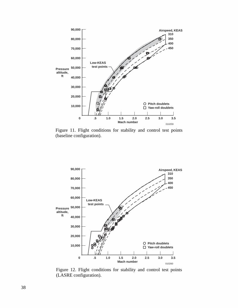
38

Low-KEAS test points

010259

Pressurealtitude,

ft

Airspeed, KEAS310

350

400

450

90,000

80,000

70,000

60,000

50,000

40,000

30,000

20,000

10,000

0 .5 1.0 1.5 2.0Mach number

2.5 3.0 3.5

Pitch doubletsYaw-roll doublets

Figure 11. Flight conditions for stability and control test points(baseline configuration).

Low-KEAS test points

010260

Airspeed, KEAS310

350

400

450

90,000

80,000

70,000

60,000

50,000

40,000

30,000

20,000

10,000

0 .5 1.0 1.5 2.0Mach number

2.5 3.0 3.5

Pitch doubletsYaw-roll doublets

Pressurealtitude,

ft

Figure 12. Flight conditions for stability and control test points(LASRE configuration).

39

Low-KEAS test points

010261

Airspeed, KEAS310

350

400

450

90,000

80,000

70,000

60,000

50,000

40,000

30,000

20,000

10,000

0 .5 1.0 1.5 2.0Mach number

2.5 3.0 3.5

Pitch doubletsYaw-roll doublets

Pressurealtitude,

ft

Figure 13. Flight conditions for stability and control test points (testbed configuration).

40

010262

3

0

–3

2

0

–2

5

3

4

1

3

0

–3

6

4

2

2.0

1.5

1.0

.50 2 4 6

δe,

deg

ηe,

in.

α,deg

θ,deg

q,deg/sec

an,g

0 0Time, sec

010312Time, sec

010311Time, sec

2

3

0

–3

2

0

–4

5

3

4

1

4

2

–4

6

4

2

1.5

1.0

.5

δe,

deg

ηe,

in.

α,deg

θ,deg

q,deg/sec

an,g

2

3

0

–3

2

0

–6

5

4

3

3

0

6

–3

7

4

1.5

1.0

.5

δe,

deg

ηe,

in.

α,deg

θ,deg

q,deg/sec

an,g

–2

–4–2

0

–2

5

2 4 6 2 4 6 8

Measured valuepEst estimate

Measured valuepEst estimate

Measured valuepEst estimate

(a) Mach 0.6 and analtitude of 6000 ft.

(b) Mach 1.06 and analtitude of 27,900 ft.

(c) Mach 2.99 and analtitude of 80,100 ft.

Figure 14. Baseline configuration longitudinal maneuver time histories.

41

CNb

010313

.5

–.10

–.05

0

–.05

–.10

–.151.00 1.5

Mach number2.0 2.5 3.0 3.5

Cmb

010263

.5

.020

1.00 1.5 2.0 2.5 3.0 3.5

.015

.010

.005

0

–.005

–.010

Mach number

Test points

High-KEAS

Low-KEAS

Test points

High-KEAS

Low-KEAS

(a) .CNb

Figure 15. Flight-determined longitudinal coefficient biases (baseline configuration).

(b) .Cmb

42

CNα,

deg–1

Cmα,

deg–1

010314

.5

.06

.05

.03

.04

.02

.01

1.00 1.5Mach number

2.0 2.5 3.0 3.5

010264

.5

4 x 10–3

1.00 1.5 2.0 2.5 3.0 3.5–6

Mach number

High-KEAS

Low-KEAS

High-KEAS (predicted)

Low-KEAS (predicted)

3

2

1

0

–1

–2

–3

–4

–5

Test points

High-KEAS

Low-KEAS

High-KEAS (predicted)

Low-KEAS (predicted)

Test points

(a) .CNα

(b) (moment reference at 0.25 c).Cmα

Figure 16. Predicted and flight-determined angle-of-attack derivatives(baseline configuration).

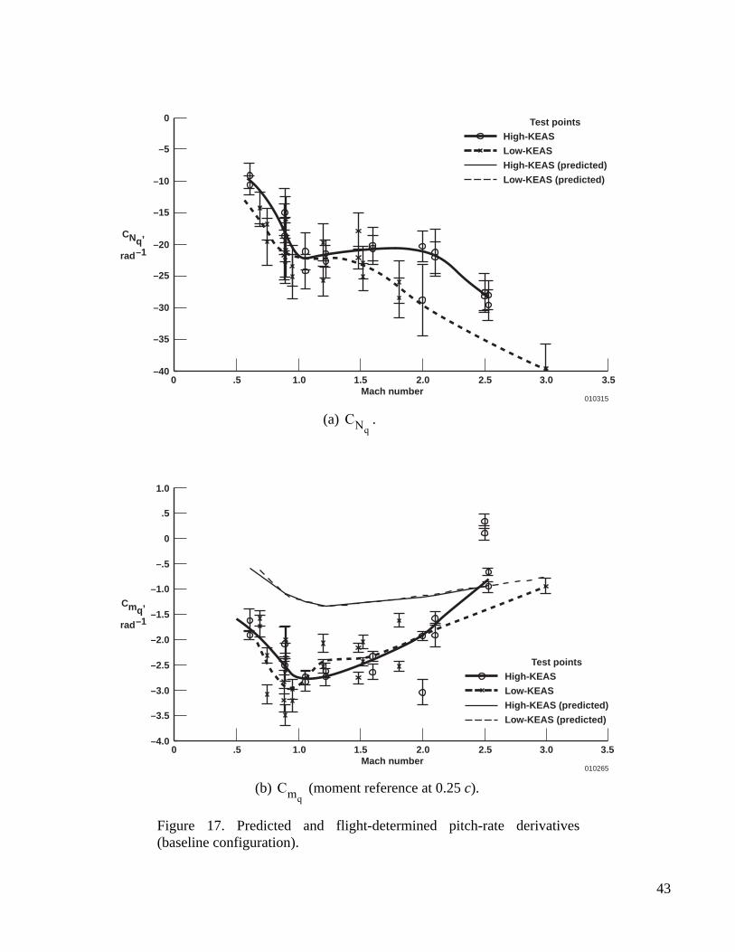
43

010315

.50 1.0

0

1.5Mach number

2.0 2.5 3.0 3.5

010265

.5 1.00 1.5 2.0 2.5 3.0 3.5–4.0

Mach number

.5

0

1.0

–.5

–1.0

–1.5

–2.0

–2.5

–3.0

–3.5

–5

–10

–15

–20

–25

–30

–35

–40

CNq,

rad–1

Cmq,

rad–1

High-KEAS

Low-KEAS

High-KEAS (predicted)

Low-KEAS (predicted)

Test points

High-KEAS

Low-KEAS

High-KEAS (predicted)

Low-KEAS (predicted)

Test points

(a) .CNq

(b) (moment reference at 0.25 c).Cmq

Figure 17. Predicted and flight-determined pitch-rate derivatives(baseline configuration).

44

CNδe,

deg–1

Cmδe,

deg–1

010316

.50 1.0

.015

1.5Mach number

2.0 2.5 3.0 3.5

010266

.5 1.00 1.5 2.0 2.5 3.0 3.5Mach number

0 x 10–3

.010

.005

0

–.005

–.010

–1

–2

–3

–4

–5

–6

–7

High-KEAS

Low-KEAS

High-KEAS (predicted)

Low-KEAS (predicted)

Test points

High-KEAS

Low-KEAS

High-KEAS (predicted)

Low-KEAS (predicted)

Test points

(a) .CNδe

(b) (moment reference at 0.25 c).Cmδe

Figure 18. Predicted and flight-determined elevator derivatives(baseline configuration).

45

Figure 19. LASRE configuration longitudinal maneuver time histories.

(a) Mach 0.5 and analtitude of 12,000 ft.

(b) Mach 1.03 and analtitude of 26,800 ft.

(c) Mach 1.73 and analtitude of 43,600 ft.

010267

4

–2

8

3

0

–3

8

6

4

1.4

0 2

δe,

deg

ηe,

in.

α,deg

θ,deg

q,deg/sec

an,g

0

5

3

0

–3

7

6

5

4

δe,

deg

ηe,

in.

α,deg

θ,deg

q,deg/sec

an,g

4

5

0

6.5

δe,

deg

ηe,

in.

α,deg

θ,deg

q,deg/sec

an,g

0 2 4 0 2 4Time, sec

010318Time, sec

010317Time, sec

2

0

2

–2

0

2

–4

0

–2

2

–4

0

–2

6

4

1.0

.6

1.4

1.0

.6

1.4

1.0

.6

2

–2

3

2

4

3

2

4

3

2

–2

6.0

5.5

5.0

4 6 8

Measured valuepEst estimate

Measured valuepEst estimate

Measured valuepEst estimate

46

CNb

010319

–.10

–.05

0

–.05

–.10

–.150

Mach number

Cmb

.020

0

.015

.010

.005

0

–.005

–.010

.2 .4 .6 .8 1.0 1.2 1.4 1.6 1.8 2.0

010268Mach number

.2 .4 .6 .8 1.0 1.2 1.4 1.6 1.8 2.0

Test points

High-KEAS

Low-KEAS

Test points

High-KEAS

Low-KEAS

(a) .CNb

Figure 20. Flight-determined longitudinal coefficient biases (LASRE configuration).

(b) .Cmb

47

Cmα,

deg–1

010269

3

1.0Mach number

4 x 10–3

2

1

0

–1

–2

–3

–4

–5

–60 .2 .4 .6 .8 1.2 1.4 1.6 1.8 2.0

CNα,

deg–1

010320

.05

1.0Mach number

.04

.03

.02

.01

0 .2 .4 .6 .8 1.2 1.4 1.6 1.8 2.0

.06 Test points

High-KEAS

Low-KEAS

Test points

High-KEAS

Low-KEAS

(a) .CNα

(b) (moment reference at 0.25 c).Cmα

Figure 21. Flight-determined angle-of-attack derivatives (LASRE configuration).

48

010321

0 .2Mach number

0

0

1.0

–5

–10

–15

–20

–25

–30

–35

–40.4 .6 .8 1.0 1.2 1.4 1.6 1.8 2.0

010270

.2Mach number

.4 .6 .8 1.0 1.2 1.4 1.6 1.8 2.0

.5

0

–.5

–1.0

–1.5

–2.0

–2.5

–3.0

–3.5

–4.0

Cmq,

rad–1

CNq,

rad–1

Test points

High-KEAS

Low-KEAS

Test points

High-KEAS

Low-KEAS

(a) .CNq

(b) (moment reference at 0.25 c).Cmq

Figure 22. Flight-determined pitch rate derivatives (LASRE configuration).

49

010322

.015

.010

.005

0

–.005

–.0100

Mach number

–6

.2 .4 .6 .8 1.0 1.2 1.4 1.6 1.8 2.0

010271

0Mach number

.2 .4 .6 .8 1.0 1.2 1.4 1.6 1.8 2.0–7

–5

–4

–3

–2

–1

0 x 10–3

Cmδe,

deg–1

CNδe,

deg–1

Test points

High-KEAS

Low-KEAS

Test points

High-KEAS

Low-KEAS

(a) .CNδe

(b) (moment reference at 0.25 c).Cmδe

Figure 23. Flight-determined elevator derivatives (LASRE configuration).

50

010272

2

1

0

–1

2

0

–2

4

3

2

2

0

–2

4

3

2

1.1

1.0

.9

.8

.70 1

δe,

deg

ηe,

in.

α,deg

θ,deg

q,deg/sec

an,g

1

0

–1

–2

2

0

–4

4.0

3.5

3.0

1

0

–1

2.0

1.5

1.2

1.1

.9

δe,

deg

ηe,

in.

α,deg

θ,deg

q,deg/sec

an,g

2

1

0

–1

3

2

0

4.5

4.0

2.5

2

0

–2

5.5

5.0

3.5

1.2

1.0

.8

δe,

deg

ηe,

in.

α,deg

θ,deg

q,deg/sec

an,g

1

3.5

3.0

4.5

4.0

–2

1.0

2 3 0 2 4 0 1 2 3Time, sec

010324Time, sec

010323Time, sec

Measured valuepEst estimate

Measured valuepEst estimate

Measured valuepEst estimate

(a) Mach 0.67 and analtitude of 7,100 ft.

(b) Mach 0.97 and analtitude of 25,100 ft.

(c) Mach 3.02 and analtitude of 67,900 ft.

Figure 24. Test bed configuration longitudinal maneuver time histories.

51

Cmb

010273

.015

.020

Mach number

.010

.005

0

–.005

–.0100 .5 1.0 1.5 2.0 2.5 3.0 3.5

CNb

010325

.10

Mach number0

.05

0

–.05

–.10

–.15.5 1.0 1.5 2.0 2.5 3.0 3.5

Test points

High-KEAS

Low-KEAS

Test points

High-KEAS

Low-KEAS

(a) .CNb

(b) .Cmb

Figure 25. Flight-determined longitudinal coefficient biases (test bed configuration).

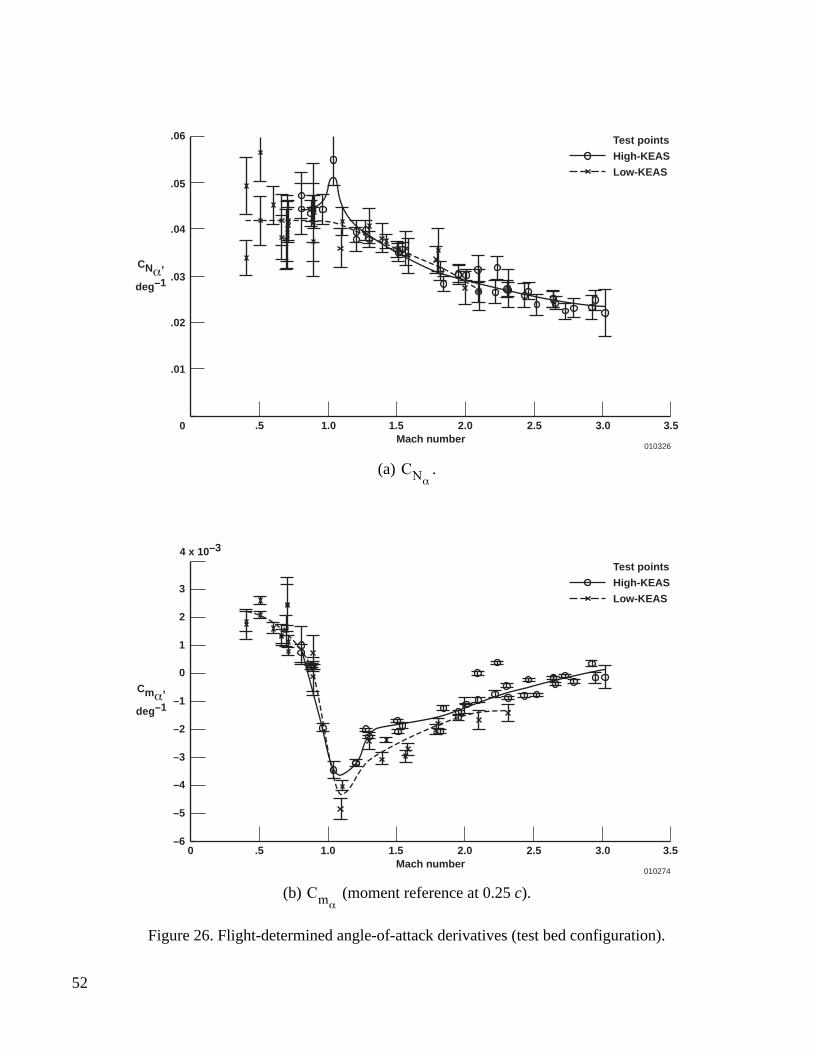
52

010274

3

Mach number

4 x 10–3

2

1

0

–1

–2

–3

–4

–5

–6.50 1.0 1.5 2.0 2.5 3.0 3.5

Cmα,

deg–1

CNα,

deg–1

Test points

High-KEAS

Low-KEAS

Test points

High-KEAS

Low-KEAS

010326

.05

.06

Mach number

.04

.03

.02

.01

0 .5 1.0 1.5 2.0 2.5 3.0 3.5

(a) .CNα

(b) (moment reference at 0.25 c).Cmα

Figure 26. Flight-determined angle-of-attack derivatives (test bed configuration).

53

1.0

.5

0

–.5

–1.0

–1.5

–2.0

–2.5

–3.0

–3.5

–4.0

010275Mach number

.5 1.0 1.5 2.0 2.5 3.0 3.50

Cmq,

rad–1

CNq,

rad–1

Test points

High-KEAS

Low-KEAS

Test points

High-KEAS

Low-KEAS

010327

0

Mach number

–5

–10

–15

–20

–25

–30

–35

–40.5 1.0 1.5 2.0 2.5 3.0 3.50

(a) .CNq

(b) (moment reference at 0.25 c).Cmq

Figure 27. Flight-determined pitch-rate derivatives (test bed configuration).

54

–1

0 x 10–3

–2

–3

–4

–5

–6

–7

010276Mach number

.5 1.0 1.5 2.0 2.5 3.0 3.50

010328

.015

.010

.005

0

–.005

–.010

Mach number.5 1.0 1.5 2.0 2.5 3.0 3.50

Test points

High-KEAS

Low-KEAS

Test points

High-KEAS

Low-KEAS

Cmδe,

deg–1

CNδe,

deg–1

(a) .CNδe

(b) (moment reference at 0.25 c).Cmδe

Figure 28. Flight-determined elevator derivatives (test bed configuration).

55

.

Pressurealtitude,

ft

90,000

80,000

70,000

60,000

50,000

40,000

30,000

20,000

10,000

010277Mach number

SR-71configuration

.5 1.0 1.5 2.0 2.5 3.0 3.50

Airspeed, KEAS310

350

400

450

BaselineLASRETest bed

Figure 29. Flight conditions for comparison of configurationlongitudinal stability and control derivatives.

56

Cmb

.020

.015

.010

.005

0

–.005

–.010

010278Mach number

.5 1.0 1.5 2.0 2.5 3.0 3.50

CNb

.10

.05

0

–.05

–.10

–.15

010329Mach number

.5 1.0 1.5 2.0 2.5 3.0 3.50

SR-71configuration

BaselineLASRETest bed

SR-71configuration

BaselineLASRETest bed

(a) .CNb

(b) .Cmb

Figure 30. Flight-determined longitudinal coefficient biases (all three configurations).

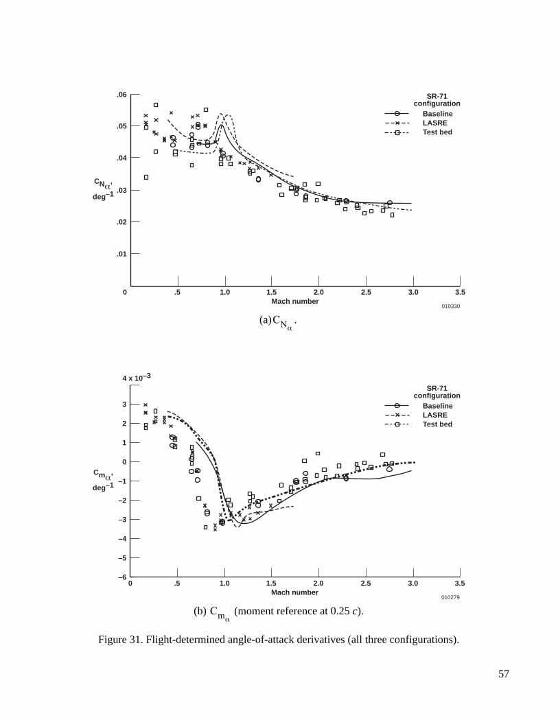
57

010279

3

4 x 10–3

2

1

0

–1

–2

–3

–4

–5

–6

Mach number.5 1.0 1.5 2.0 2.5 3.0 3.50

Cmα,

deg–1

CNα,

deg–1

SR-71configuration

BaselineLASRETest bed

SR-71configuration

BaselineLASRETest bed

010330

.06

.05

.04

.03

.02

.01

Mach number.5 1.0 1.5 2.0 2.5 3.0 3.50

(a) .CNα

(b) (moment reference at 0.25 c).Cmα

Figure 31. Flight-determined angle-of-attack derivatives (all three configurations).

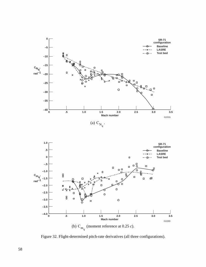
58

010280

1.0

.5

0

–.5

–1.0

–1.5

–2.0

–2.5

–3.0

–3.5

–4.0

Mach number.5 1.0 1.5 2.0 2.5 3.0 3.50

010331

0

–5

–10

–15

–20

–25

–30

–35

–40

Mach number.5 1.0 1.5 2.0 2.5 3.0 3.50

Cmq,

rad–1

CNq,

rad–1

SR-71configuration

BaselineLASRETest bed

SR-71configuration

BaselineLASRETest bed

(a) .CNq

(b) (moment reference at 0.25 c).Cmq

Figure 32. Flight-determined pitch-rate derivatives (all three configurations).

59

Cmδe,

deg–1

010281

–1

0 x 10–3

–2

–3

–4

–5

–6

–7

Mach number.5 1.0 1.5 2.0 2.5 3.0 3.50

SR-71configuration

BaselineLASRETest bed

SR-71configuration

BaselineLASRETest bed

010332

.015

.010

.005

0

–.005

–.010

Mach number.5 1.0 1.5 2.0 2.5 3.0 3.50

CNδe,

deg–1

(a) .CNδe

(b) (moment reference at 0.25 c).Cmδe

Figure 33. Flight-determined elevator derivatives (all three configurations).

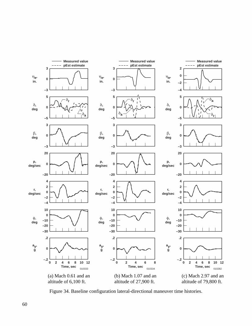
60

010282

3

0

δ,deg

ηe,

in.

β,deg

φ,deg

p,deg/sec

r,deg/sec

ay,g

Time, sec010334

Time, sec010333

Time, sec

0

–3

5

0

–5

3

0

–3

20

0

–20

4

2

0

–2

–4

10

0

–10

–20

–30

.2

0

–.2

3

δ,deg

δr δr

δrδaδa

δa

ηe,

in.

β,deg

φ,deg

p,deg/sec

r,deg/sec

ay,g

0

–3

5

0

–5

3

0

–3

20

0

–20

4

2

0

–2

–4

10

0

–10

–20

–30

.2

0

–.2

2

δ,deg

ηe,

in.

β,deg

φ,deg

p,deg/sec

r,deg/sec

ay,g

0

–4

5

0

–5

3

0

–3

20

0

–20

4

2

0

–2

–4

10

0

–10

–20

–30

.2

0

–.2

–2

2 4 6 8 10 12 0 0 2 4 6 8 10 122 4 6 8

Measured valuepEst estimate

Measured valuepEst estimate

Measured valuepEst estimate

(a) Mach 0.61 and analtitude of 6,100 ft.

(b) Mach 1.07 and analtitude of 27,900 ft.

(c) Mach 2.97 and analtitude of 79,800 ft.

Figure 34. Baseline configuration lateral-directional maneuver time histories.

61

Mach number010283

3

0

Cnb

.5 1.0 1.5 2.0 2.5 3.0 3.5

4 x 10–3

Mach number010335

.015

0

CYb

.5 1.0 1.5 2.0 2.5 3.0 3.5

Mach number010336

1.0

0

Clb

.5 1.0 1.5 2.0 2.5 3.0 3.5

1.5 x 10–3

.010

.005

0

–.005

–.010

–.015

.5

0

–.5

–1.0

2

1

0

–1

Test points

High-KEAS

Low-KEAS

Test points

High-KEAS

Low-KEAS

Test points

High-KEAS

Low-KEAS

(a) .CYb

(b) .Clb

(c) .Cnb

Figure 35. Flight-determined lateral-directional coefficient biases (baselineconfiguration).

62

Mach number010284

0

Cnβ,

deg–1

.5 1.0 1.5 2.0 2.5 3.0 3.5

2.5 x 10–3

Mach number010337

–.002

0

CYβ,

deg–1

.5 1.0 1.5 2.0 2.5 3.0 3.5

Mach number010338

0

0

Clβ,

deg–1

.5 1.0 1.5 2.0 2.5 3.0 3.5

.5 x 10–3

0

–.004

–.006

–.008

–.010

–.012

–.5

–1.0

–1.5

–2.0

–2.5

2.0

1.5

1.0

.5

High-KEASLow-KEASHigh-KEAS (predicted)Low-KEAS (predicted)

Test points

High-KEASLow-KEASHigh-KEAS (predicted)Low-KEAS (predicted)

Test points

High-KEASLow-KEASHigh-KEAS (predicted)Low-KEAS (predicted)

Test points

(a) .CYβ

(b) .Clβ

(c) (moment reference at 0.25 c).Cnβ

Figure 36. Predicted and flight-determined angle-of-sideslip derivatives (baselineconfiguration).

63

Mach number010285

.20

0 .5 1.0 1.5 2.0 2.5 3.0 3.5

Mach number010339

1.5

0

CYp,

rad–1

.5 1.0 1.5 2.0 2.5 3.0 3.5

Mach number010340

.10

0 .5 1.0 1.5 2.0 2.5 3.0 3.5

1.0

.5

0

–.5

.05

0

–.05

–.10

–.15

–.20

–.25

–.30

.15

.10

.05

0

–.05

–.10

–.15

–.20

Clp,

rad–1

Cnp,

rad–1

High-KEASLow-KEASHigh-KEAS (predicted)Low-KEAS (predicted)

Test points

High-KEASLow-KEAS

Test points

High-KEASLow-KEASHigh-KEAS (predicted)Low-KEAS (predicted)

Test points

High-KEAS (predicted)Low-KEAS (predicted)

Test points

(a) .CYp

(b) .Clp

(c) (moment reference at 0.25 c).Cnp

Figure 37. Predicted and flight-determined roll-rate derivatives (baselineconfiguration).

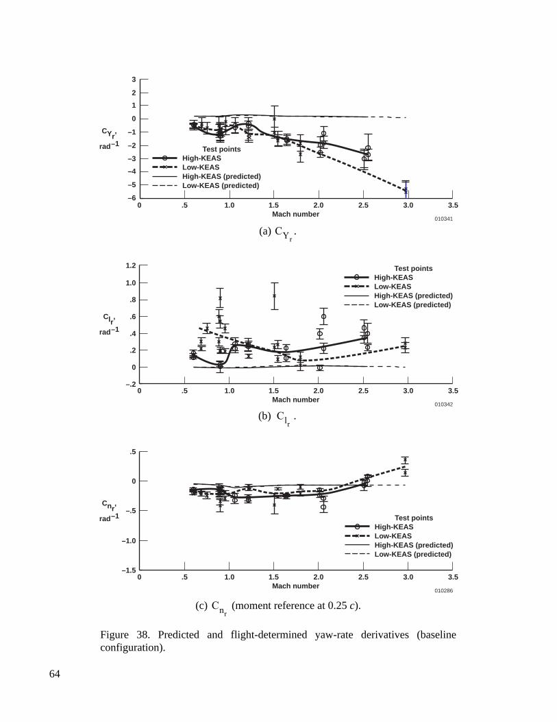
64

Mach number010286

.5

0 .5 1.0 1.5 2.0 2.5 3.0 3.5

Mach number010341

3

0

CYr,

rad–1

.5 1.0 1.5 2.0 2.5 3.0 3.5

Mach number010342

1.2

0 .5 1.0 1.5 2.0 2.5 3.0 3.5

2

1

0

–1

–2

–3

–4

–5

–6

1.0

.8

.6

.4

.2

0

–.2

0

–.5

–1.0

–1.5

High-KEASLow-KEASHigh-KEAS (predicted)Low-KEAS (predicted)

Test points

High-KEASLow-KEASHigh-KEAS (predicted)Low-KEAS (predicted)

Test points

High-KEASLow-KEASHigh-KEAS (predicted)Low-KEAS (predicted)

Test points

Clr,

rad–1

Cnr,

rad–1

(a) .CYr

(b) .Clr

(c) (moment reference at 0.25 c).Cnr

Figure 38. Predicted and flight-determined yaw-rate derivatives (baselineconfiguration).

65

Mach number010287

–.5

0 .5 1.0 1.5 2.0 2.5 3.0 3.5

0 x 10–3

Mach number010343

4

0

CYδr,

deg–1

.5 1.0 1.5 2.0 2.5 3.0 3.5

5 x 10–3

Mach number010344

3

0 .5 1.0 1.5 2.0 2.5 3.0 3.5

4 x 10–4

3

2

1

2

1

0

–1

–2

–3

–4

–1.0

–1.5

–2.0

Clδr,

deg–1

Cnδr,

deg–1

High-KEASLow-KEASHigh-KEAS (predicted)Low-KEAS (predicted)

Test points

High-KEASLow-KEASHigh-KEAS (predicted)Low-KEAS (predicted)

Test points

High-KEASLow-KEASHigh-KEAS (predicted)Low-KEAS (predicted)

Test points

(a) .CYδr

(b) .Clδr

(c) (moment reference at 0.25 c).Cnδr

Figure 39. Predicted and flight-determined rudder derivatives (baselineconfiguration).

66

Mach number010288

4

0 .5 1.0 1.5 2.0 2.5 3.0 3.5

6 x 10–4

Mach number010345

2

0

CYδa,

deg–1

.5 1.0 1.5 2.0 2.5 3.0 3.5

3 x 10–3

1

0

–1

–2

–3

Mach number010346

0 .5 1.0 1.5 2.0 2.5 3.0 3.5

2.5 x 10–3

2.0

1.5

1.0

.5

2

0

–2

–4

Clδa,

deg–1

Cnδa,

deg–1

High-KEASLow-KEASHigh-KEAS (predicted)Low-KEAS (predicted)

Test points

High-KEASLow-KEASHigh-KEAS (predicted)Low-KEAS (predicted)

Test points

High-KEASLow-KEASHigh-KEAS (predicted)Low-KEAS (predicted)

Test points

(a) .CYδa

(b) .Clδa

(c) (moment reference at 0.25 c).Cnδa

Figure 40. Predicted and flight-determined aileron derivatives (baselineconfiguration).

67

010289

0 2

δ,deg

δa

δr

δa

δr δaδr

ηa,

in.

β,deg

φ,deg

r,deg/sec

p,deg/sec

ay,g

Time, sec010348

Time, sec010347

Time, sec4 6 8 0 2 4 6 8 10 12 0 2 4 6 8

2

0

–2

3

0

–3

2

0

–2

10

0

–10

2

0

–2

5

0

–5

.06

0

–.06

δ,deg

ηa,

in.

β,deg

φ,deg

r,deg/sec

p,deg/sec

ay,g

2

0

–2

3

0

–3

2

0

–2

10

0

–10

2

0

–2

5

0

–5

.06

0

–.06

δ,deg

ηa,

in.

β,deg

φ,deg

r,deg/sec

p,deg/sec

ay,g

2

0

–2

3

0

–3

2

0

–2

10

0

–10

3

1

2

0

–1

20

15

10

.06

0

–.06

Measured valuepEst estimate

Measured valuepEst estimate

Measured valuepEst estimate

(a) Mach 0.60 and analtitude of 15,100 ft.

(b) Mach 0.95 and analtitude of 27,500 ft.

(c) Mach 1.74 and analtitude of 44,000 ft.

Figure 41. LASRE configuration lateral-directional maneuver time histories.

68

Mach number010290

3

0 .2

Cnb

4 x 10–3

.015

CYb

1.0

Clb

1.5 x 10–3

.010

.005

0

–.005

–.010

–.015

.5

0

–.5

–1.0

2

1

0

–1.4 .6 .8 1.0 1.2 1.4 1.6 1.8 2.0

Mach number010350

0 .2 .4 .6 .8 1.0 1.2 1.4 1.6 1.8 2.0

Mach number010349

0 .2 .4 .6 .8 1.0 1.2 1.4 1.6 1.8 2.0

Test points

High-KEAS

Low-KEAS

Test points

High-KEAS

Low-KEAS

Test points

High-KEAS

Low-KEAS

(a) .CYb

(b) .Clb

(c) .Cnb

Figure 42. Flight-determined lateral-directional coefficient biases (LASREconfiguration).

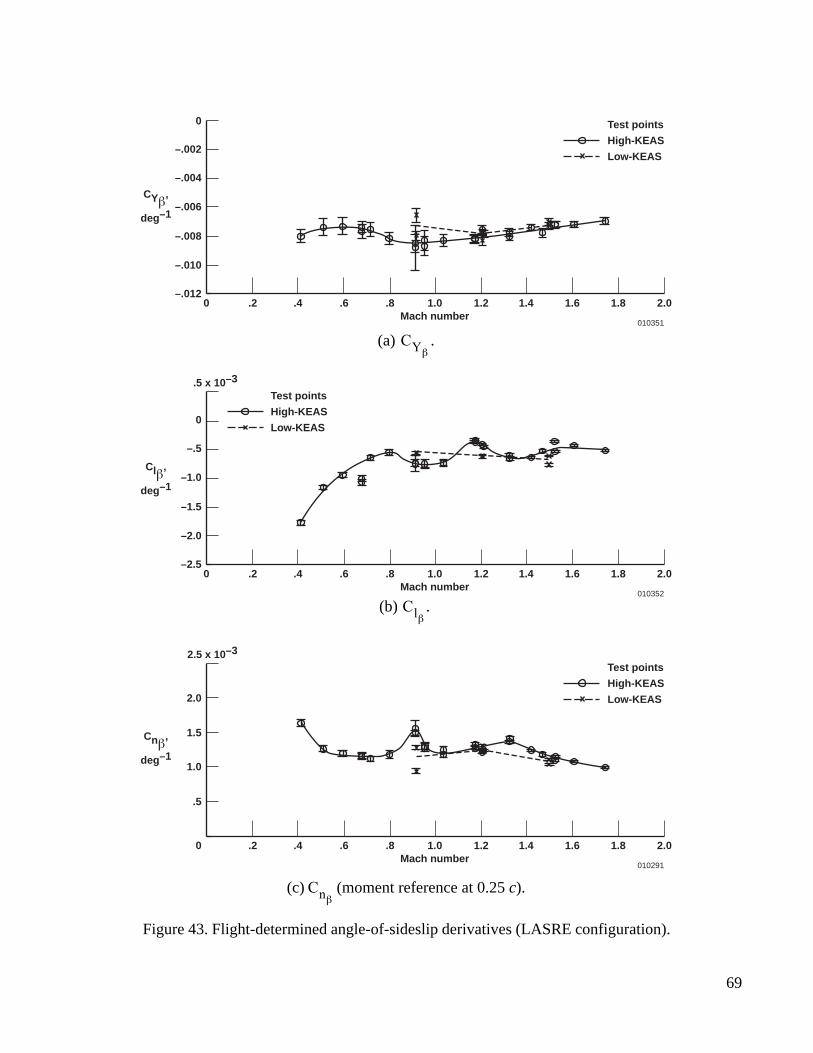
69

2.0

Cnβ,

deg–1

2.5 x 10–3

0

–.002

0

CYβ,

deg–1

–.004

–.006

–.008

–.010

–.012

0

Clβ,

deg–1

.5 x 10–3

–.5

–1.0

–1.5

–2.0

–2.5

Mach number010291

.2 .4 .6 .8 1.0 1.2 1.4 1.6 1.8 2.0

Mach number010352

0 .2 .4 .6 .8 1.0 1.2 1.4 1.6 1.8 2.0

Mach number010351

0 .2 .4 .6 .8 1.0 1.2 1.4 1.6 1.8 2.0

1.5

1.0

.5

Test points

High-KEAS

Low-KEAS

Test points

High-KEAS

Low-KEAS

Test points

High-KEAS

Low-KEAS

(a) .CYβ

(b) .Clβ

(c) (moment reference at 0.25 c).Cnβ

Figure 43. Flight-determined angle-of-sideslip derivatives (LASRE configuration).

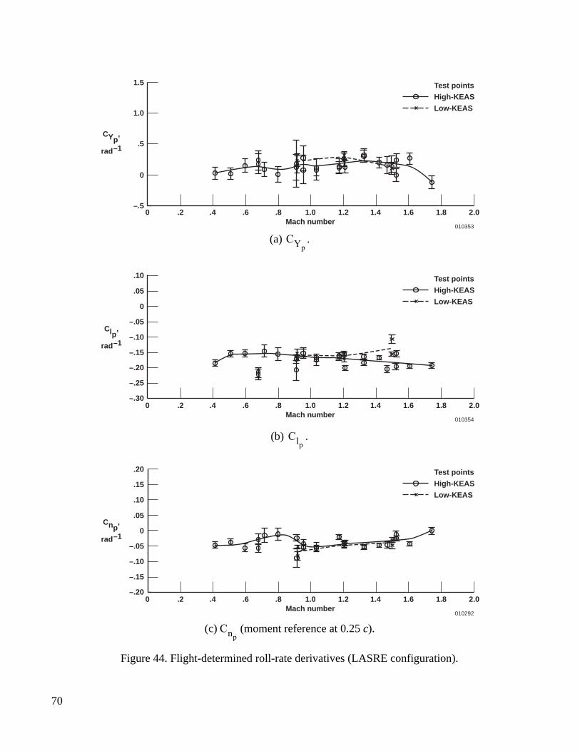
70

Cnp,

rad–1

1.5

CYp,

rad–1

Clp,

rad–1

Mach number010292

0 .2 .4 .6 .8 1.0 1.2 1.4 1.6 1.8 2.0

Mach number010354

0 .2 .4 .6 .8 1.0 1.2 1.4 1.6 1.8 2.0

Mach number010353

0 .2 .4 .6 .8 1.0 1.2 1.4 1.6 1.8 2.0

.10

.05

0

–.05

–.10

–.15

–.20

1.0

.5

0

–.5

–.25

–.30

.10

.05

0

–.05

–.10

–.15

–.20

.15

.20

Test points

High-KEAS

Low-KEAS

Test points

High-KEAS

Low-KEAS

Test points

High-KEAS

Low-KEAS

(a) .CYp

(b) .Clp

(c) (moment reference at 0.25 c).Cnp

Figure 44. Flight-determined roll-rate derivatives (LASRE configuration).

71

.5

3

1.2

Mach number010293

0 .2 .4 .6 .8 1.0 1.2 1.4 1.6 1.8 2.0

Mach number010356

0 .2 .4 .6 .8 1.0 1.2 1.4 1.6 1.8 2.0

Mach number010355

0 .2 .4 .6 .8 1.0 1.2 1.4 1.6 1.8 2.0

2

1

0

–1

–2

–3

–4

–5

–6

1.0

.8

.6

.4

.2

0

–.2

0

–.5

–1.0

–1.5

Test points

High-KEAS

Low-KEAS

CYr,

rad–1

Test points

High-KEAS

Low-KEAS

Test points

High-KEAS

Low-KEAS

Clr,

rad–1

Cnr,

rad–1

(a) .CYr

(b) .Clr

(c) (moment reference at 0.25 c).Cnr

Figure 45. Flight-determined yaw-rate derivatives (LASRE configuration).

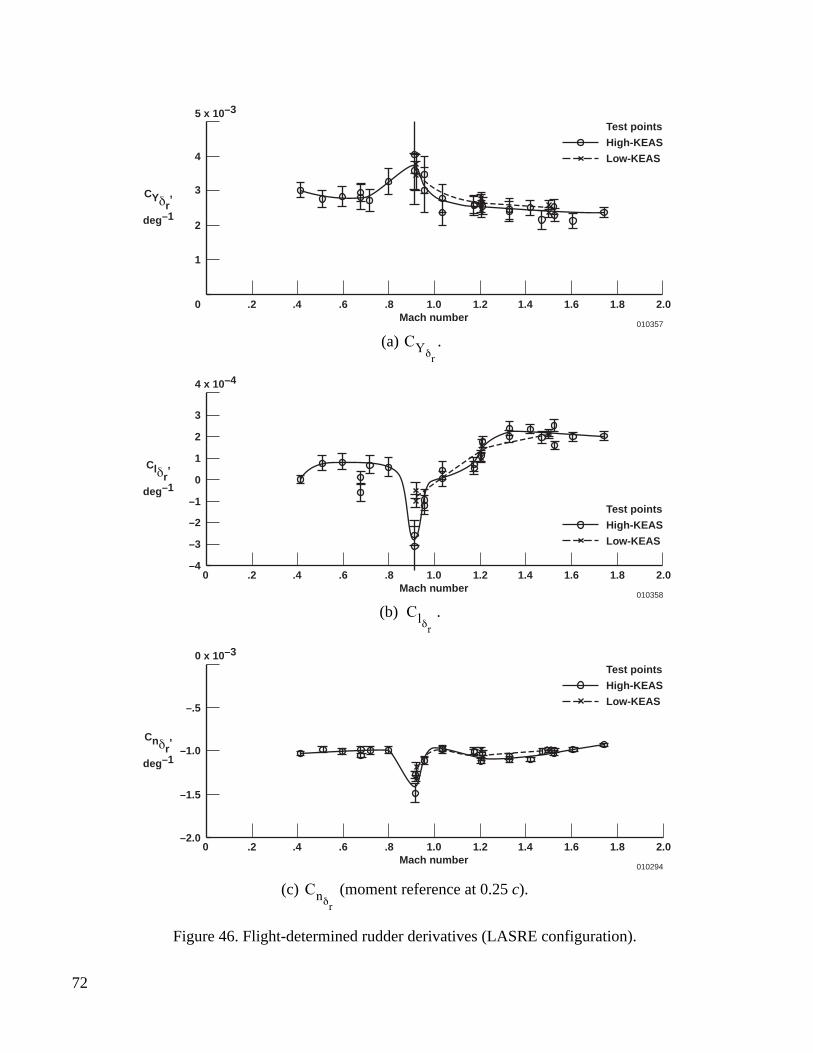
72

–.5

0 x 10–3

4

5 x 10–3

3

4 x 10–4

Mach number010294

0 .2 .4 .6 .8 1.0 1.2 1.4 1.6 1.8 2.0

Mach number010358

0 .2 .4 .6 .8 1.0 1.2 1.4 1.6 1.8 2.0

Mach number010357

0 .2 .4 .6 .8 1.0 1.2 1.4 1.6 1.8 2.0

3

2

1

2

1

0

–1

–2

–3

–4

–1.0

–1.5

–2.0

Test points

High-KEAS

Low-KEAS

Test points

High-KEAS

Low-KEAS

Test points

High-KEAS

Low-KEAS

CYδr,

deg–1

Clδr,

deg–1

Cnδr,

deg–1

(a) .CYδr

(b) .Clδr

(c) (moment reference at 0.25 c).Cnδr

Figure 46. Flight-determined rudder derivatives (LASRE configuration).

73

4

6 x 10–4

2

3 x 10–3

1

0

–1

–2

–3

2.0

2.5 x 10–3

Mach number010295

0 .2 .4 .6 .8 1.0 1.2 1.4 1.6 1.8 2.0

Mach number010360

0 .2 .4 .6 .8 1.0 1.2 1.4 1.6 1.8 2.0

Mach number010359

0 .2 .4 .6 .8 1.0 1.2 1.4 1.6 1.8 2.0

1.5

1.0

.5

2

0

–4

–2

Test points

High-KEAS

Low-KEAS

Test points

High-KEAS

Low-KEAS

Test points

High-KEAS

Low-KEAS

CYδa,

deg–1

Clδa,

deg–1

Cnδa,

deg–1

(a) .CYδa

(b) .Clδa

(c) (moment reference at 0.25 c).Cnδa

Figure 47. Flight-determined aileron derivatives (LASRE configuration).

74

010296

0 2

δ,deg

ηa,

in.

β,deg

φ,deg

r,deg/sec

p,deg/sec

ay,g

Time, sec010362

Time, sec010361

Time, sec4 6 8 0 2 4 6 8 10 12 0 2 4 6 8

2

0

–2

3

0

–3

1

0

–1

1510

–5

50

–10

2

0

–2

–10

–15

–25

.02

0

–.06

δ,deg

ηa,

in.

β,deg

φ,deg

r,deg/sec

p,deg/sec

ay,g

2

0

–2

3

0

–3

1

0

–1

10

0

–10

2

0

–2

0

–5

–10

δ,deg

ηa,

in.

β,deg

φ,deg

r,deg/sec

p,deg/sec

ay,g

1

–1

–3

3

0

–3

1

0

–1

10

0

–10

2

0

–2

35

30

25

0

–.04

–.08

0

–2

–20

–.02

–.04

.02

0

–.06

–.02

–.04

Measured valuepEst estimate

Measured valuepEst estimate

Measured valuepEst estimate

δa

δr

δa

δr

δa

δr

(a) Mach 0.71 and analtitude of 20,000 ft.

(b) Mach 1.06 and analtitude of 25,500 ft.

(c) Mach 3.01 and analtitude of 68,300 ft.

Figure 48. Test bed configuration lateral-directional maneuver time histories.

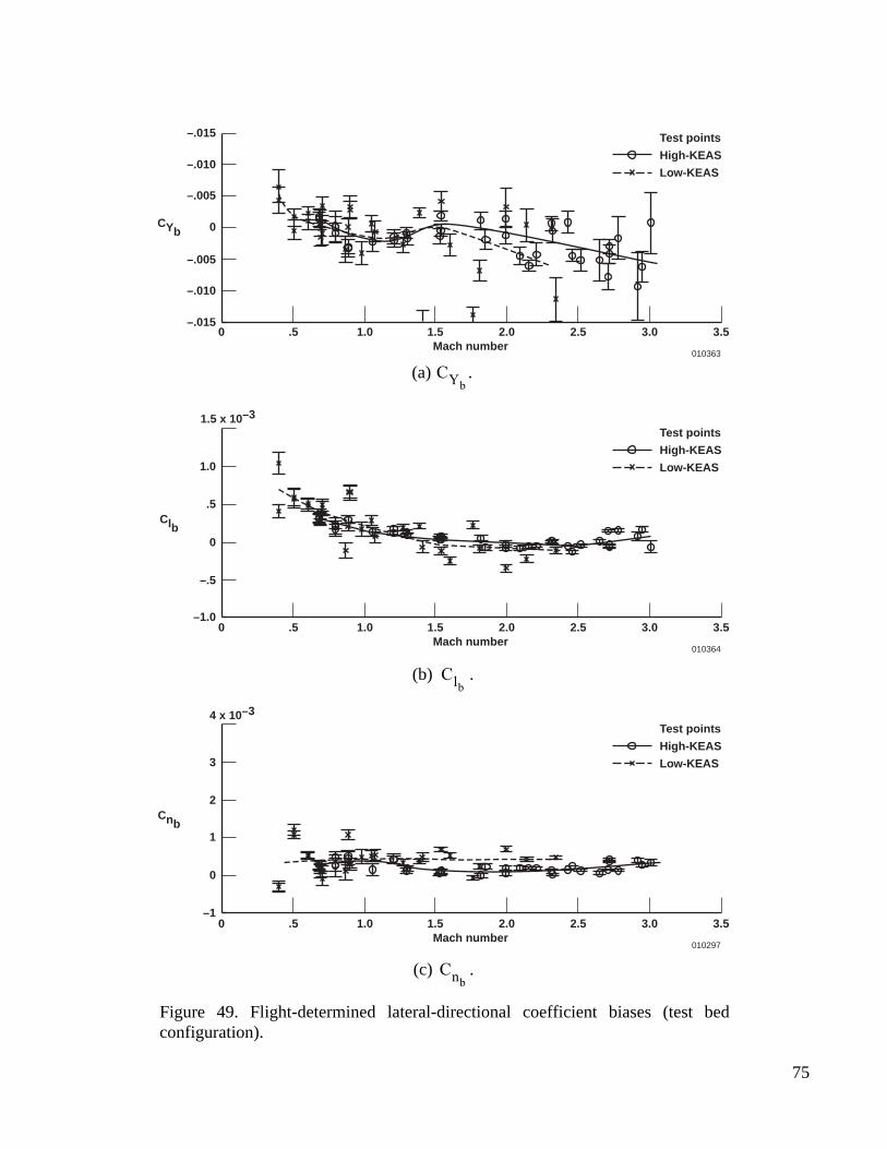
75

3

Cnb

4 x 10–3

–.015

CYb

1.0

Clb

1.5 x 10–3

–.010

–.005

0

–.005

–.010

–.015

Mach number010364

0 .5 1.0 1.5 2.0 2.5 3.0 3.5

Mach number010363

0 .5 1.0 1.5 2.0 2.5 3.0 3.5

Mach number010297

0 .5 1.0 1.5 2.0 2.5 3.0 3.5

.5

0

–.5

–1.0

2

1

0

–1

Test points

High-KEAS

Low-KEAS

Test points

High-KEAS

Low-KEAS

Test points

High-KEAS

Low-KEAS

(a) .CYb

(b) .Clb

(c) .Cnb

Figure 49. Flight-determined lateral-directional coefficient biases (test bedconfiguration).

76

Mach number010298

2.0

Cnβ,

deg–1

.5 1.0 1.5 2.0 2.5 3.0 3.5

2.5 x 10–3

Mach number010365

0

0

CYβ,

deg–1

.5 1.0 1.5 2.0 2.5 3.0 3.5

Mach number010366

0

0

Clβ,

deg–1

.5 1.0 1.5 2.0 2.5 3.0 3.5

.5 x 10–3

–.5

–1.0

–1.5

–2.0

–2.5

–.002

–.004

–.006

–.008

–.010

–.012

1.5

1.0

.5

0

Test points

High-KEAS

Low-KEAS

Test points

High-KEAS

Low-KEAS

Test points

High-KEAS

Low-KEAS

(a) .CYβ

(b) .Clβ

(c) (moment reference at 0.25 c).Cnβ

Figure 50. Flight-determined angle-of-sideslip derivatives (test bed configuration).

77

Mach number010299

.20

0 .5 1.0 1.5 2.0 2.5 3.0 3.5

Mach number010367

1.5

0 .5 1.0 1.5 2.0 2.5 3.0 3.5–.5

Mach number010368

.10

0 .5 1.0 1.5 2.0 2.5 3.0 3.5–.30

1.0

.5

0

.05

0

–.05

–.10

–.15

–.20

–.25

.15

.10

.5

0

–.5

–.10

–.15

–.20

Test points

High-KEAS

Low-KEAS

Test points

High-KEAS

Low-KEAS

Test points

High-KEAS

Low-KEAS

CYp,

rad–1

Clp,

rad–1

Cnp,

rad–1

(a) .CYp

(b) .Clp

(c) (moment reference at 0.25 c).Cnp

Figure 51. Flight-determined roll-rate derivatives (test bed configuration).

78

Mach number010300

.5

0 .5 1.0 1.5 2.0 2.5 3.0 3.5

Mach number010369

3

0 .5 1.0 1.5 2.0 2.5 3.0 3.5

Mach number010370

1.2

0 .5 1.0 1.5 2.0 2.5 3.0 3.5

2

1

0

–1

–2

–3

–4

–5

–6

1.0

.8

.6

.4

.2

0

–.2

0

–.5

–1.0

–1.5

Test points

High-KEAS

Low-KEAS

Test points

High-KEAS

Low-KEAS

CYr,

rad–1

Clr,

rad–1

Cnr,

rad–1

Test points

High-KEAS

Low-KEAS

(a) .CYr

(b) .Clr

(c) (moment reference at 0.25 c).Cnr

Figure 52. Flight-determined yaw-rate derivatives (test bed configuration).

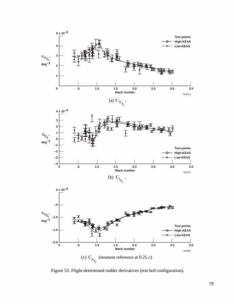
79

Mach number010301

–.5

0 .5 1.0 1.5 2.0 2.5 3.0 3.5

0 x 10–3

Mach number010371

4

0 .5 1.0 1.5 2.0 2.5 3.0 3.5

5 x 10–3

Mach number010372

3

0 .5 1.0 1.5 2.0 2.5 3.0 3.5

4 x 10–4

3

2

1

2

1

0

–1

–2

–3

–4

–1.0

–1.5

–2.0

CYδr,

deg–1

Test points

High-KEAS

Low-KEAS

Test points

High-KEAS

Low-KEAS

Test points

High-KEAS

Low-KEAS

Clδr,

deg–1

Cnδr,

deg–1

(a) .CYδr

(b) .Clδr

(c) (moment reference at 0.25 c).Cnδr

Figure 53. Flight-determined rudder derivatives (test bed configuration).

80

Mach number010302

4

0 .5 1.0 1.5 2.0 2.5 3.0 3.5

6 x 10–4

–4

Mach number010373

2

0 .5 1.0 1.5 2.0 2.5 3.0 3.5

3 x 10–3

1

0

–1

–2

–3

Mach number010374

2.0

0 .5 1.0 1.5 2.0 2.5 3.0 3.5

2.5 x 10–3

1.5

1.0

.5

2

0

–2

CYδa,

deg–1

Test points

High-KEAS

Low-KEAS

Clδa,

deg–1

Cnδa,

deg–1

Test points

High-KEAS

Low-KEAS

Test points

High-KEAS

Low-KEAS

(a) .CYδa

(b) .Clδa

(c) (moment reference at 0.25 c).Cnδa

Figure 54. Flight-determined aileron derivatives (test bed configuration).

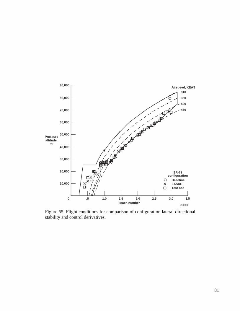
81

Airspeed, KEAS

310

350

400

450

80,000

90,000

60,000

40,000

20,000

0 .5 1.0 1.5Mach number

010303

2.0 2.5 3.0 3.5

Pressurealtitude,

ft

SR-71configuration

BaselineLASRETest bed

70,000

50,000

30,000

10,000

Figure 55. Flight conditions for comparison of configuration lateral-directionalstability and control derivatives.

82

Mach number010304

3

0

Cnb

.5 1.0 1.5 2.0 2.5 3.0 3.5

4 x 10–3

–1

Mach number010375

.010

.015

0

CYb

.5 1.0 1.5 2.0 2.5 3.0 3.5

.005

0

–.005

–.010

–.015

Mach number010376

0

Clb

.5 1.0 1.5 2.0 2.5 3.0 3.5

1.5 x 10–3

1.0

2

1

0

.5

0

–.5

–1.0

SR-71configuration

BaselineLASRETest bed

SR-71configuration

BaselineLASRETest bed

SR-71configuration

BaselineLASRETest bed

(a) .CYb

(b) .Clb

(c) .Cnb

Figure 56. Flight-determined lateral-directional coefficient biases (all threeconfigurations).

83

Mach number010305

2.0

0

Cnβ,

deg–1

.5 1.0 1.5 2.0 2.5 3.0 3.5

2.5 x 10–3

Mach number010377

0

0

CYβ,

deg–1

.5 1.0 1.5 2.0 2.5 3.0 3.5–.012

Mach number010378

0

0

Clβ,

deg–1

.5 1.0 1.5 2.0 2.5 3.0 3.5

.5 x 10–3

–.5

–1.0

–1.5

–2.0

–2.5

–.002

–.004

–.006

–.008

–.010

1.5

1.0

.5

SR-71configuration

BaselineLASRETest bed

SR-71configuration

BaselineLASRETest bed

SR-71configuration

BaselineLASRETest bed

(a) .CYβ

(b) .Clβ

(c) (moment reference at 0.25 c).Cnβ

Figure 57. Flight-determined angle-of-sideslip derivatives (all threeconfigurations).

84

Mach number010306

.20

0 .5 1.0 1.5 2.0 2.5 3.0 3.5–.20

Mach number010379

1.5

0 .5 1.0 1.5 2.0 2.5 3.0 3.5–.5

Mach number010380

.10

0 .5 1.0 1.5 2.0 2.5 3.0 3.5–.30

1.0

.5

0

.05

0

–.05

–.10

–.15

–.20

–.25

.15

.10

.05

0

–.05

–.10

–.15

SR-71configuration

BaselineLASRETest bed

CYp,

rad–1

Clp,

rad–1

Cnp,

rad–1

SR-71configuration

BaselineLASRETest bed

SR-71configuration

BaselineLASRETest bed

(a) .CYp

(b) .Clp

(c) (moment reference at 0.25 c).Cnp

Figure 58. Flight-determined roll-rate derivatives (all three configurations).

85

Mach number010307

.5

0 .5 1.0 1.5 2.0 2.5 3.0 3.5–1.5

Mach number010381

3

0 .5 1.0 1.5 2.0 2.5 3.0 3.5–6

Mach number010382

1.2

0 .5 1.0 1.5 2.0 2.5 3.0 3.5–.2

2

1

0

–1

–2

–3

–4

–5

1.0

.8

.6

.4

.2

0

0

–.5

–1.0

SR-71configuration

BaselineLASRETest bed

CYr,

rad–1

Clr,

rad–1

Cnr,

rad–1

SR-71configuration

BaselineLASRETest bed

SR-71configuration

BaselineLASRETest bed

(a) .CYr

(b) .Clr

(c) (moment reference at 0.25 c).Cnr

Figure 59. Flight-determined yaw-rate derivatives (all three configurations).

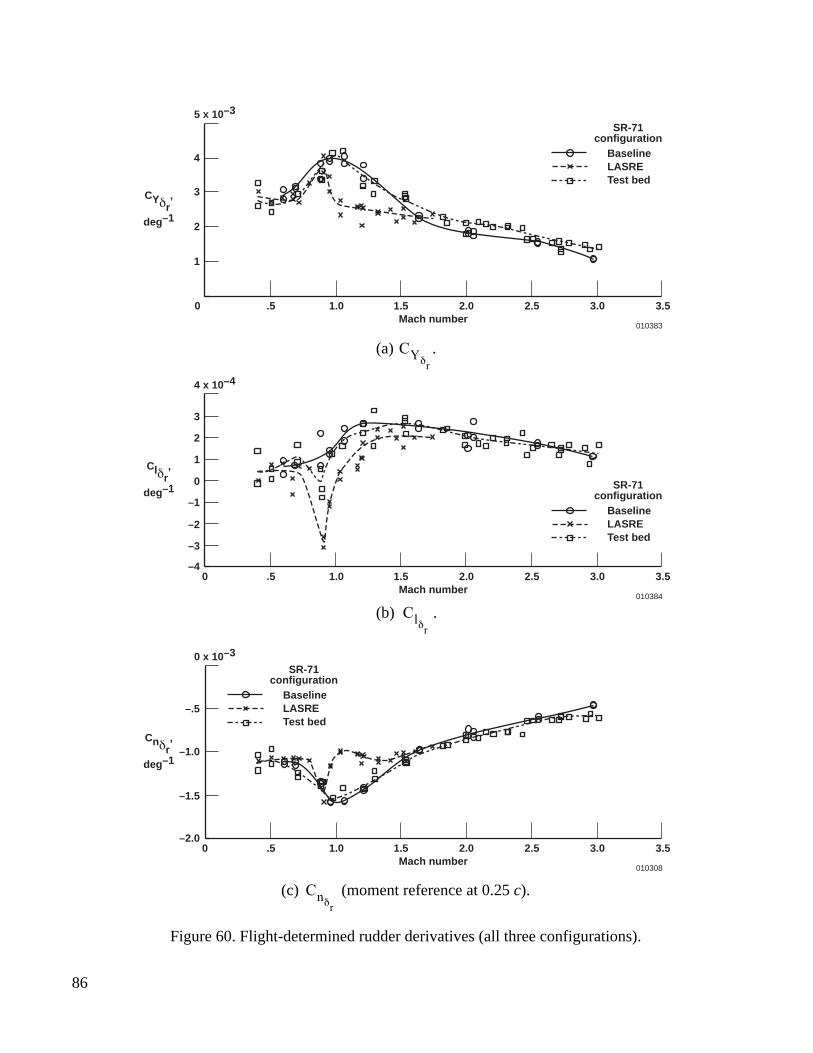
86

Mach number010308

0 .5 1.0 1.5 2.0 2.5 3.0 3.5

0 x 10–3

–2.0

–.5

Mach number010383

0 .5 1.0 1.5 2.0 2.5 3.0 3.5

5 x 10–3

4

Mach number010384

0 .5 1.0 1.5 2.0 2.5 3.0 3.5

4 x 10–4

–4

3

3

2

1

2

1

0

–1

–2

–3

–1.0

–1.5

CYδr,

deg–1

SR-71configuration

BaselineLASRETest bed

Clδr,

deg–1

Cnδr,

deg–1

SR-71configuration

BaselineLASRETest bed

SR-71configuration

BaselineLASRETest bed

(a) .CYδr

(b) .Clδr

(c) (moment reference at 0.25 c).Cnδr

Figure 60. Flight-determined rudder derivatives (all three configurations).

87

Mach number010309

4

0 .5 1.0 1.5 2.0 2.5 3.0 3.5

6 x 10–4

–4

Mach number010385

2

0 .5 1.0 1.5 2.0 2.5 3.0 3.5

3 x 10–3

1

0

–1

–2

–3

Mach number010386

0 .5 1.0 1.5 2.0 2.5 3.0 3.5

2.5 x 10–3

2.0

1.5

1.0

.5

2

0

–2

SR-71configuration

BaselineLASRETest bed

CYδa,

deg–1

Clδa,

deg–1

Cnδa,

deg–1

SR-71configuration

BaselineLASRETest bed

SR-71configuration

BaselineLASRETest bed

(a) .CYδa

(b) .Clδa

(c) (moment reference at 0.25 c).Cnδa

Figure 61. Flight-determined aileron derivatives (all three configurations).

REPORT DOCUMENTATION PAGE

Form ApprovedOMB No. 0704-0188

Public reporting burden for this collection of information is estimated to average 1 hour per response, including the time for reviewing instructions, searching existing data sources, gathering andmaintaining the data needed, and completing and reviewing the collection of information. Send comments regarding this burden estimate or any other aspect of this collection of information,including suggestions for reducing this burden, to Washington Headquarters Services, Directorate for Information Operations and Reports, 1215 Jefferson Davis Highway, Suite 1204, Arlington,VA 22202-4302, and to the Office of Management and Budget, Paperwork Reduction Project (0704-0188), Washington, DC 20503.

1. AGENCY USE ONLY (Leave blank) 2. REPORT DATE 3. REPORT TYPE AND DATES COVERED

4. TITLE AND SUBTITLE 5. FUNDING NUMBERS

6. AUTHOR(S)

8. PERFORMING ORGANIZATION REPORT NUMBER

7. PERFORMING ORGANIZATION NAME(S) AND ADDRESS(ES)

9. SPONSORING/MONITORING AGENCY NAME(S) AND ADDRESS(ES) 10. SPONSORING/MONITORING AGENCY REPORT NUMBER

11. SUPPLEMENTARY NOTES

12a. DISTRIBUTION/AVAILABILITY STATEMENT 12b. DISTRIBUTION CODE

13. ABSTRACT (Maximum 200 words)

14. SUBJECT TERMS 15. NUMBER OF PAGES

16. PRICE CODE

17. SECURITY CLASSIFICATION OF REPORT

18. SECURITY CLASSIFICATION OF THIS PAGE

19. SECURITY CLASSIFICATION OF ABSTRACT

20. LIMITATION OF ABSTRACT

NSN 7540-01-280-5500 Standard Form 298 (Rev. 2-89)

Prescribed by ANSI Std. Z39-18298-102

Stability and Control Estimation Flight Test Results for the SR-71Aircraft With Externally Mounted Experiments

WU 710-35-14-E8-OM-00-844

Timothy R. Moes and Kenneth Iliff

NASA Dryden Flight Research CenterP.O. Box 273Edwards, California 93523-0273

H-2465

National Aeronautics and Space AdministrationWashington, DC 20546-0001 NASA/TP-2002-210718

A maximum-likelihood output-error parameter estimation technique is used to obtain stability andcontrol derivatives for the NASA Dryden Flight Research Center SR-71A airplane and forconfigurations that include experiments externally mounted to the top of the fuselage. This research isbeing done as part of the envelope clearance for the new experiment configurations. Flight data areobtained at speeds ranging from Mach 0.4 to Mach 3.0, with an extensive amount of test points atapproximately Mach 1.0. Pilot-input pitch and yaw-roll doublets are used to obtain the data. Thisreport defines the parameter estimation technique used, presents stability and control derivativeresults, and compares the derivatives for the three configurations tested. The experimentalconfigurations studied generally show acceptable stability, control, trim, and handling qualitiesthroughout the Mach regimes tested. The reduction of directional stability for the experimentalconfigurations is the most significant aerodynamic effect measured and identified as a designconstraint for future experimental configurations. This report also shows the significant effects ofaircraft flexibility on the stability and control derivatives.

Control derivatives, Maximum likelihood estimates, Parameter identification,SR-71, Stability derivatives

A03

94

Unclassified Unclassified Unclassified Unlimited

June 2002 Technical Publication

Unclassified—UnlimitedSubject Category 08

This report is available at http://www.dfrc.nasa.gov/DTRS/