International Journal of Environmental Monitoring and Analysis 2015; 3(6-1): 47-55

Published online October 15, 2015 (http://www.sciencepublishinggroup.com/j/ijema)

doi: 10.11648/j.ijema.s.2015030601.16

ISSN: 2328-7659 (Print); ISSN: 2328-7667 (Online)

Estimation of Coastal Stability Due to Coastal Structures

Huseyin Murat Cekirge

Department of Mechanical Engineering, the Grove School of Engineering, the City College of the City University of New York, New York,

USA

Email address: hmcekirge@usa.net

To cite this article: Huseyin Murat Cekirge. Estimation of Coastal Stability Due to Coastal Structures.International Journal of Environmental Monitoring and

Analysis.Special Issue: Environmental Social Impact Assessment (ESIA) and Risk Assessment of Crude Oil and Gas Pipelines.

Vol. 3, No. 6-1, 2015, pp. 47-55.doi: 10.11648/j.ijema.s.2015030601.16

Abstract: The coastal structures are unavoidable for various industrial operations. These are changing hydrodynamics of the

marine and its adjacent areas; and are directly influencing environmental conditions of the marine environment. The

sedimentation on shorelines is strongly under influence of the new structures. The methodology, which is introduced in the paper,

is a comparative study of situation of sediments before and after constructing the coastal installations. It is a guiding tool for

planners to find the influences of the new structures in the marine area.

Keywords: Coastal Stability, Erosion of Sediments on Coastal Shores, Deposition of Sediments on Coastal Shores,

Marine Sediment Model

1. Introduction

This paper addresses concerns about the potential effects of

a new coastal structure on coastal stability of the adjacent

marine area. There are always environmental concerns about

the impact of the new coastal structures on coastal areas. The

monitoring agencies always consider the ecological

consequences of accelerated shallowing resulting from

alterations in sediment transport dynamics following the

construction of the new coastal structure. The ESIA reports are

always wondering the effects of coastal structures which will

be constructed in marine areas. It is expected that the new

structure affects hydrodynamics of the coast and it may cause

of change of coastal line due to erosion and sedimentation. It

is necessary to analyze effects of the coastal structure on

present hydrodynamics and forecast the potential changes of

coastal line using suitable hydrodynamic simulation model.

Countermeasures against the impacts should be provided in

accordance with the simulation results taking into

consideration of environmental protection.

Geo-morphological changes focuses on observations of

coastal sedimentation and the need to determine the potential

changes in sediment transport, after the new coastal structure

is built. The hypothesis of limited long-shore transport is

consistent with the minimal sand build up at the existing

coastal structure. The potential impacts due to the new coastal

structure are:

� changes in wave patterns;

� changes in currents;

� changes in sediment transport;

� changes in coastal orientation; and

� secondary impacts on coastal dunes.

As a result, the building party committed to carrying out a

study to further investigate the effects of the new coastal

structure development on the existing hydrodynamic

conditions, alongshore littoral transport rates, and offshore

(sub-littoral) sediment transport patterns. The paper is

addressed herein in the following:

Determining the potential effects of the solid-core coastal

structure on the area’s coastal stability and focusing on

potential changes to the erosional/depositional condition of

the shoreline.

This process entails field study and wave refraction

modeling. An area, Figure 1 and 2, with metrological, wave

conditions and sea bottom topography (bathymetry) are

selected.

48 Huseyin Murat Cekirge. Estimation of Coastal Stability Due to Coastal Structures

Figure 1. Location of the new coastal structure at marine area, [1].

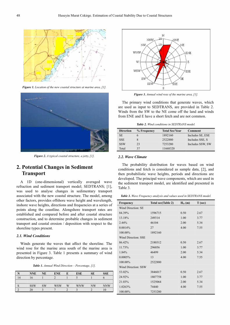
Figure 2. A typical coastal structure, a jetty, [1].

2. Potential Changes in Sediment

Transport

A 1D (one-dimensional) vertically averaged wave

refraction and sediment transport model; SEDTRANS; [1],

was used to analyse changes in sedimentary transport

associated with the new coastal structure. The model, among

other factors, provides offshore wave height and wavelength,

inshore wave heights, directions and frequencies at a series of

points along the coastline. Alongshore transport rates are

established and compared before and after coastal structure

construction, and to determine probable changes in sediment

transport and coastal erosion / deposition with respect to the

shoreline types present.

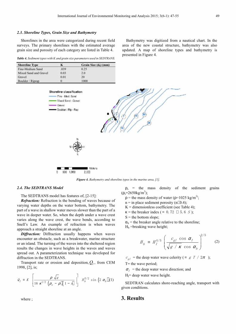
2.1. Wind Conditions

Winds generate the waves that affect the shoreline. The

wind rose for the marine area south of the marine area is

presented in Figure 3. Table 1 presents a summary of wind

direction by percentage.

Table 1. Annual Wind Direction – Percentage, [1].

N NNE NE ENE E ESE SE SSE

14 16 1 2 1 5 1 6

S SSW SW WSW W WNW NW NNW

2 20 3 7 2 3 2 10

Figure 3. Annual wind rose of the marine area, [1].

The primary wind conditions that generate waves, which

are used as input to SEDTRANS, are provided in Table 2.

Winds from the SW to the NE come off the land and winds

from ENE and E have a short fetch and are not common.

Table 2. Wind conditions in SEDTRANS model.

Direction % Frequency Total Sec/Year Comment

SE 6 1892160 Includes SE, ESE

SSE 8 2522880 Includes SSE, S

SSW 23 7253280 Includes SSW, SW

Total 37 11668320

2.2. Wave Climate

The probability distribution for waves based on wind

conditions and fetch is considered as sample data, [2], and

then probabilistic wave heights, periods and directions are

developed. The principal wave components, which are used in

the sediment transport model, are identified and presented in

Table 3.

Table 3. Wave Frequency analysis and values used in SEDTRANS model.

Frequency Total sec(Table 2) HO (m) T (sec)

Wind Direction: SE

84.39% 1596715 0.50 2.67

13.18% 249314 1.00 3.77

2.44% 46104 2.00 5.34

0.0014% 27 4.00 7.55

100.00% 1892160

Wind Direction: SSE

86.42% 2180312 0.50 2.67

11.73% 296056 1.00 3.77

1.84% 46499 2.00 5.34

0.0005% 13 4.00 7.55

100.00% 2522880

Wind Direction: SSW

53.02% 3846017 0.50 2.67

24.92% 1807758 1.00 3.77

21.03% 1525064 2.00 5.34

1.0263% 74440 4.00 7.55

100.00% 7253280

International Journal of Environmental Monitoring and Analysis 2015; 3(6-1): 47-55 49

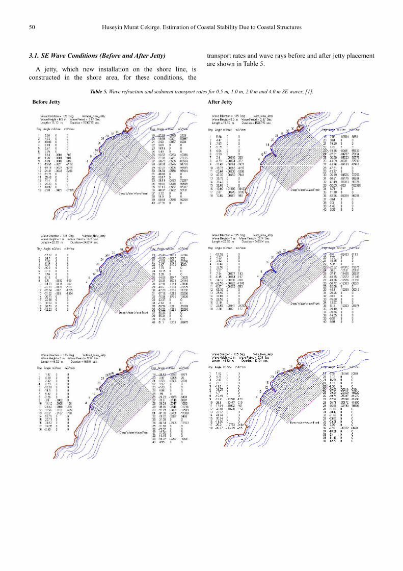
2.3. Shoreline Types, Grain Size and Bathymetry

Shorelines in the area were categorized during recent field

surveys. The primary shorelines with the estimated average

grain size and porosity of each category are listed in Table 4.

Table 4. Sediment types with K and grain size parameters used in SEDTRANS.

Shoreline Type K Grain Size (d0) (mm)

Fine-Medium Sand .039 0.25

Mixed Sand and Gravel 0.03 2.0

Gravel 0.01 20

Boulder / Riprap 0 1000

Bathymetry was digitized from a nautical chart. In the

area of the new coastal structure, bathymetry was also

updated. A map of shoreline types and bathymetry is

presented in Figure 4.

Figure 4. Bathymetry and shoreline types in the marine area, [1].

2.4. The SEDTRANS Model

The SEDTRANS model has features of, [2-15]:

Refraction: Refraction is the bending of waves because of

varying water depths on the water bottom, bathymetry. The

part of a wave in shallow water moves slower than the part of a

wave in deeper water. So, when the depth under a wave crest

varies along the wave crest, the wave bends, according to

Snell’s Law. An example of refraction is when waves

approach a straight shoreline at an angle.

Diffraction: Diffraction usually happens when waves

encounter an obstacle, such as a breakwater, marine structure

or an island. The turning of the waves into the sheltered region

results the changes in wave heights in the waves and waves

spread out. A parameterization technique was developed for

diffraction in the SEDTRANS.

Transport rate or erosion and deposition, lQ , from CEM

1998, [2], is;

( ) ( )( )5/2

1/2sin 2

16 1l b b

s

gQ K H

n

ρ ακ ρ ρ

= − −

(1)

where ;

ρs = the mass density of the sediment grains

(ρs=2650kg/m3);

ρ = the mass density of water (ρ=1025 kg/m3)

;

n = in place sediment porosity (n≅0.4);

K = dimensionless coefficient (see Table 4);

κ = the breaker index ( 0.72 5.6 S= + );

S = the bottom slope;

αb = the breaker angle relative to the shoreline;

Hb =breaking wave height;

2/5

4/5cos

/ cos

gl Ib I

b

cH H

g

α

κ α

=

(2)

glc = the deep water wave celerity ( / 2g T π= );

T= the wave period;

Iα = the deep water wave direction; and

HI= deep water wave height.

SEDTRAN calculates shore-reaching angle, transport with

given conditions.

3. Results

50 Huseyin Murat Cekirge. Estimation of Coastal Stability Due to Coastal Structures

3.1. SE Wave Conditions (Before and After Jetty)

A jetty, which new installation on the shore line, is

constructed in the shore area, for these conditions, the

transport rates and wave rays before and after jetty placement

are shown in Table 5.

Table 5. Wave refraction and sediment transport rates for 0.5 m, 1.0 m, 2.0 m and 4.0 m SE waves, [1].

Before Jetty After Jetty

International Journal of Environmental Monitoring and Analysis 2015; 3(6-1): 47-55 51

Before Jetty After Jetty

3.2. SSE Wave Conditions (Before and After Jetty)

For these conditions, the transport rates and wave rays

before and after jetty placement are shown in Table 6.

Table 6. Wave refraction and sediment transport rates for 0.5 m, 1.0 m, 2.0 m and 4.0 m SSE waves, [1].

Before Jetty After Jetty

52 Huseyin Murat Cekirge. Estimation of Coastal Stability Due to Coastal Structures

Before Jetty After Jetty

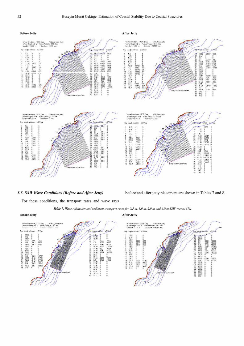
3.3. SSW Wave Conditions (Before and After Jetty)

For these conditions, the transport rates and wave rays

before and after jetty placement are shown in Tables 7 and 8.

Table 7. Wave refraction and sediment transport rates for 0.5 m, 1.0 m, 2.0 m and 4.0 m SSW waves, [1].

Before Jetty After Jetty

International Journal of Environmental Monitoring and Analysis 2015; 3(6-1): 47-55 53

Before Jetty After Jetty

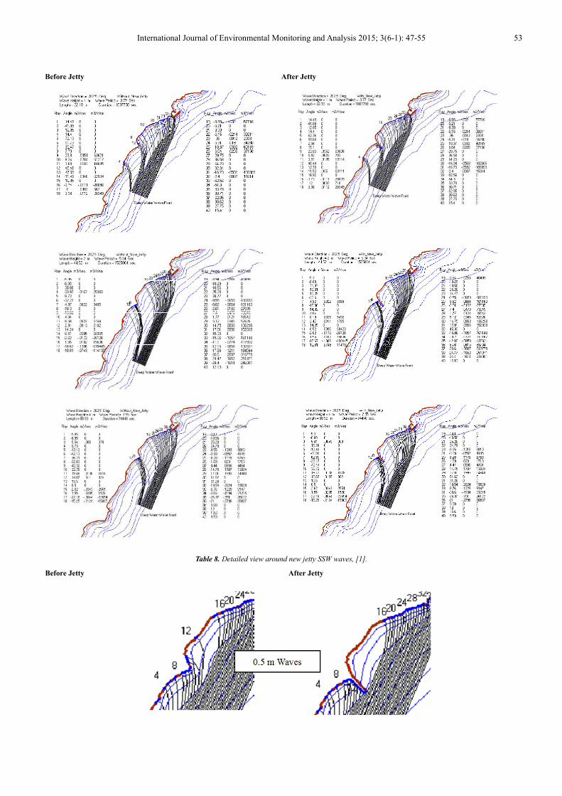
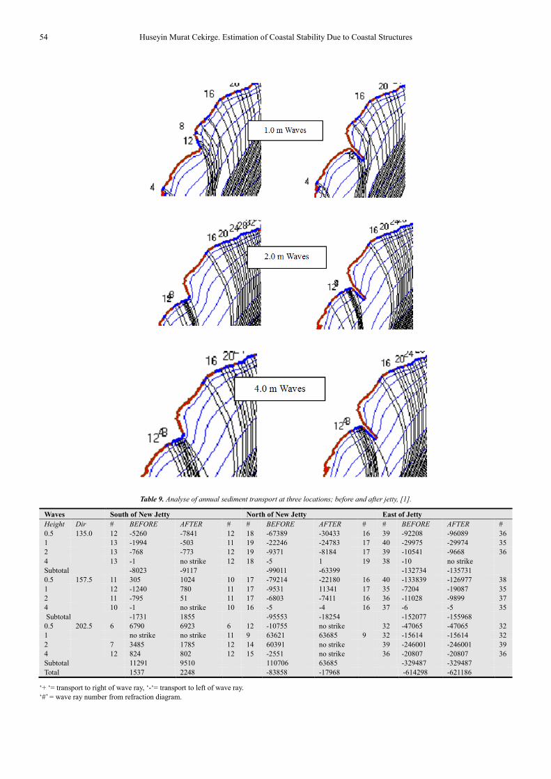
Table 8. Detailed view around new jetty SSW waves, [1].

Before Jetty After Jetty

54 Huseyin Murat Cekirge. Estimation of Coastal Stability Due to Coastal Structures

Table 9. Analyse of annual sediment transport at three locations; before and after jetty, [1].

Waves South of New Jetty North of New Jetty East of Jetty

Height Dir # BEFORE AFTER # # BEFORE AFTER # # BEFORE AFTER #

0.5 135.0 12 -5260 -7841 12 18 -67389 -30433 16 39 -92208 -96089 36

1 13 -1994 -503 11 19 -22246 -24783 17 40 -29975 -29974 35

2 13 -768 -773 12 19 -9371 -8184 17 39 -10541 -9668 36

4 13 -1 no strike 12 18 -5 1 19 38 -10 no strike

Subtotal -8023 -9117 -99011 -63399 -132734 -135731

0.5 157.5 11 305 1024 10 17 -79214 -22180 16 40 -133839 -126977 38

1 12 -1240 780 11 17 -9531 11341 17 35 -7204 -19087 35

2 11 -795 51 11 17 -6803 -7411 16 36 -11028 -9899 37

4 10 -1 no strike 10 16 -5 -4 16 37 -6 -5 35

Subtotal -1731 1855 -95553 -18254 -152077 -155968

0.5 202.5 6 6790 6923 6 12 -10755 no strike 32 -47065 -47065 32

1 no strike no strike 11 9 63621 63685 9 32 -15614 -15614 32

2 7 3485 1785 12 14 60391 no strike 39 -246001 -246001 39

4 12 824 802 12 15 -2551 no strike 36 -20807 -20807 36

Subtotal 11291 9510 110706 63685 -329487 -329487

Total 1537 2248 -83858 -17968 -614298 -621186

‘+ ‘= transport to right of wave ray, ‘-‘= transport to left of wave ray.

‘#’ = wave ray number from refraction diagram.

International Journal of Environmental Monitoring and Analysis 2015; 3(6-1): 47-55 55

4. Discussion of Results

It is seen that there are no changes in wave rays before and

after jetty placement for waves coming from the SSE and SE

because of the alignment of the jetty with the approaching

waves. SSW waves show some shadowing due to the jetty,

which is evident under the 0.5 m and 1.0 m waves, however

there is also a natural shadowing to the north due to the natural

refraction of SSW waves due to bathymetry, as shown under

2.0 m and 4.0 m wave conditions (Tables 7 and 8).

An analyse of the annual sediment transport rates at three

locations, south of the jetty, north of the jetty, and surrounding

are presented in Table 9. Results of this analysis indicate:

� No net change east of the jetty,

� No net change south of the jetty.

� Several changes north of the jetty:

� Less transport southward with waves from SE and

SSE.

� Less northward transport with SSW waves due to

shadow zone.

� Less annual transport to the south.

In detail analysis, these conclusions are not altered

significantly by analyzing the shoreline with the jetty and

surrounding by using the SEDTRANS model. In other words,

there are no significant expected changes in annual

sedimentary transport along shorelines adjacent to the new

jetty, see Table 9. The transport north of the jetty has

decreased because this area is being sheltered by the jetty.

However, annual sedimentary transport has not been changed,

and the shorelines are expected to remain stable with the jetty

and surrounding.

References

[1] H. M. Cekirge, Sediment Transport on Shorelines, Maltepe Uni., Int. Rep. 4, Istanbul, 2010.

[2] CEM, Coastal Engineering Manual, Department of the Army, Corps of Engineers Washington, DC, 1998.

[3] W. Bascom, W. Waves and beaches: the dynamics of the ocean surface. Garden City, NY: Doubleday & Co., Inc., 1964.

[4] P. Komar, Beach processes and sedimentation. Englewood Cliffs, NJ: Prentice-Hall, Inc., 1976.

[5] G. Dean and R.A. Dalrymple, Water wave mechanics for engineers and scientists. Singapore: World Scientific, 1991.

[6] M. B. Abbott, H. M. Petersen, and O. Skovgaard, On the Numerical Modelling of Short Waves in Shallow Water, Journal of Hydraulic Research 16, 3, 173–203, 1978.

[7] Earl J. Hayter, John M. Hamrick, Brian R. Bicknell, and Mark H. Gray, One-Dimensional Hydrodynamic/Sediment, Transport Model for Stream Networks, EPA/600/R-01/072, September 2001

[8] L. O. Amoudry and A. J. Souza (2011), Impact of sediment‐induced stratification and turbulence closures on sediment transport and morphological modelling, Cont. Shelf Res., 31, 912–928, 2011.

[9] M. Blaas, C. Dong, P. Marchesiello, J. C. McWilliams, and K. D. Stolzenbach (2007), Sediment‐ transport modeling on Southern Californian shelves: A ROMS case study, Cont. Shelf Res., 27, 832–853, 2007.

[10] A. F. Blumberg, A Primer for ECOMSED, Version 1.3, users manual, HydroQual, Inc., Mahwah, N. J, 2002

[11] H. J. de Vriend, 2D mathematical modelling of morphological evolutions in shallow water, Coastal Eng., 11, 1–27. 1987.

[12] H. J. de Vriend, and J. S. Ribberink, A quasi ‐ 3D mathematical model of coastal morphology, in Proceedings of the 21st International Conference on Coastal Engineering, edited by B. L. Edge, pp. 1689–1703, Am. Soc. of Civ. Eng., Reston, Va., 1988.

[13] US Army Corps of Engineer, Predicting Deposition Patterns in Small Basins, TP-133, March 1991.

[14] Yu-Min Wang, Jan-Mou Leu, Seydou Traore, Chou-Ping Yang, Lian-Tsai Deng and Tso-Hsin Weng, Apprehending the potential effect of sediment deposition due to dredging in Laonong River upstream, Southern Taiwan, International Journal of the Physical Sciences Vol. 5(14), pp. 2135-2142, 4 November, 2010.

[15] Edited by Wolfgang Summer and Desmond E. Walling, Modelling Erosion, Sediment Transport and Sediment Yield, A contribution to IHP-V Projects 2.1 and 6.2, International Hydrological Programme, I HP-VI, Technical Documents in Hydrology, No. 60 UNESCO, Paris, 2002.