SÉRIE ÉTUDES ET DOCUMENTS

C E N T R E D ' É T U D E S E T D E R E C H E R C H E S S U R L E D E V E L O P P E M E N T I N T E R N A T I O N A L

SÉRIE ÉTUDES ET DOCUMENTS

School or work? The role of weather shocks in Madagascar

Francesca Marchetta David E. Sahn Luca Tiberti

Études et Documents n° 3

April 2018

To cite this document:

Marchetta F., Sahn D. E., Tiberti Luca (2018) “ School or work? The role of weather shocks in Madagascar”, Études et Documents, n° 3, CERDI. http://cerdi.org/production/show/id/1917/type_production_id/1

CERDI 65 BD. F. MITTERRAND 63000 CLERMONT FERRAND – FRANCE TEL. + 33 4 73 17 74 00 FAX + 33 4 73 17 74 28 www.cerdi.org

http://cerdi.org/production/show/id/1917/type_production_id/1

http://www.cerdi.org/

Études et Documents n° 3, CERDI, 2018

2

The authors

Francesca Marchetta, Associate Professor, School of Economics and Centre d’Etude et de Recherche sur le Développement International (CERDI), UMR CNRS 6587, University of Clermont Auvergne, Clermont-Ferrand, France. E-mail: [email protected] David E. Sahn, Professor, Cornell University, USA. E-mail: [email protected]

Luca Tiberti, Assistant Professor, PEP, Université Laval, Québec, Canada. E-mail: [email protected] Corresponding author: Francesca Marchetta.

This work was supported by the LABEX IDGM+ (ANR-10-LABX-14-01) within the program “Investissements d’Avenir” operated by the French National Research Agency (ANR).

Études et Documents are available online at: http://www.cerdi.org/ed

Director of Publication: Grégoire Rota-Graziosi Editor: Catherine Araujo Bonjean Publisher: Mariannick Cornec ISSN: 2114 - 7957

Disclaimer:

Études et Documents is a working papers series. Working Papers are not refereed, they constitute research in progress. Responsibility for the contents and opinions expressed in the working papers rests solely with the authors. Comments and suggestions are welcome and should be addressed to the authors.

mailto:[email protected]



http://www.cerdi.org/ed


3

Abstract We examine the impact of rainfall variability and cyclones on schooling and work among a cohort of teens and young adults by estimating a bivariate probit model, using a panel survey conducted in 2004 and 2011 in Madagascar—a poor island nation that is frequently affected by extreme weather events. Our results show that negative rainfall deviations and cyclones reduce the current and lagged probability of attending school and encourage young men and, to a greater extent, women to enter the work force. Less wealthy households are most likely to experience this school-to-work transition in the face of rainfall shocks. The finding is consistent with poorer households having less savings and more limited access to credit and insurance, which reduces their ability to cope with negative weather shocks. Keywords Climate shocks, Employment, Schooling, Africa. JEL Codes Q54, J43, I25. Acknowledgments The authors would like to thank Olivier Santoni for the excellent work in the preparation of rainfall and cyclones data, Simone Bertoli for useful suggestions, as well as the participants to seminar presentations at LAMETA, Montpellier and at NOVAFRICA, Lisbon, to the 3rd IZA/DFID GLM-LIC Research Conference in Washington, and to the Labor and Development Workshop, Paris. Luca Tiberti acknowledges the financial support from the Partnership for Economic Policy (PEP), with funding from the Department for International Development (DFID) of the United Kingdom (or UK Aid), and the Government of Canada through the International Development Research Center (IDRC). Francesca Marchetta acknowledges the support received from the Agence Nationale de la Recherche of the French government through the program "Investissements d'avenir" (ANR-10-LABX-14-01); the usual disclaimers apply.

Introduction

Weather events can affect human capital formation and exert a long-lasting influence on individual

well-being and on macroeconomic performance. This is of particular concern in developing

countries, where high rates of poverty, a labor force primarily employed in rainfed agriculture, and

limited credit and insurance markets can magnify the effects of negative weather shocks. In this

article, we study the influence of rainfall variability and hurricanes on schooling and entry into the

labor market in Madagascar, one of the 10 countries in the world with the highest Climate Risk

Index (Kreft et al. 2016). Hurricanes, floods, and droughts are serious threats for the Malagasy

fragile ecology and agricultural sector, in which nearly three out of four workers are employed.1

According to a recent report from the US Agency for International Development (USAID),2

climate scientists expect flooding and erosion to increase in some regions of the country, as rainfall

increases in intensity; in the south, rainfall will be less predictable, leading to greater extremes,

including more frequent drought.

Our main goals are to explore (1) how normal rainfall variability affects schooling and

working decisions; (2) the extent to which there is heterogeneity across households in these

responses; and (3) the impact of acute weather shocks, particularly cyclones, on schooling and

work choices.

We focus on a cohort of young men and women in Madagascar who were between 21 and

23 years old in 2011, and who were initially surveyed in 2004. We build a balanced annual panel

data set from 2004 to 2011, with information on the school and working situation of each

individual, derived from retrospective questions included in the questionnaire of the 2011 round

1 World Development Indicators (the data refer to 2015). 2 See https://www.usaid.gov/madagascar/environment, accessed January 2018.


4

https://www.usaid.gov/madagascar/environment

of the survey. We match individual-level data with satellite-based, fine-grained information on

rainfall,3 and with data on hurricanes, using information on the time-varying place of residence of

each individual.

Our empirical analysis, based on a non-separable agricultural household conceptual

framework, involves estimating a bivariate probit model of schooling and work for the young adult

cohort members (CMs) residing in rural areas of Madagascar. We do so using time and

geographically fixed-effects. The identification strategy relies on the large temporal and spatial

historical variations in rainfall between 2004 and 2011, across 210 rural communities. Results

show that positive rainfall deviations from the long-term average increase the probability of school

enrollment, while reducing the probability of being engaged in work. We observe both

contemporaneous and lagged effects. Moreover, these effects are heterogeneous across

households. Specifically, they are attenuated when individuals are from wealthier households. This

suggests that assets help to mitigate the effect of transitory adverse weather conditions. Women

are more likely than men to be pushed to the labor market following a negative weather event. Our

results also show that cyclones reduce the probability of being enrolled in school. While we cannot

empirically test the mechanisms through which cyclones impact schooling and work decisions, a

plausible conjecture is that these rainfall events destroy roads, interrupt electricity, and damage

schools, contributing to school dropout.

This article contributes to a rapidly growing body of research, which examines how

extreme weather events influence economic outcomes (Dell, Jones, and Alken 2014), and more

specifically, human capital. Prior research has shown that weather events have a significant impact

3 Satellite-based data are preferred to those from the CRU (Climatic Research Unit), because of the poor quality of

the latter from 2006 to 2009 (see Footnote 18).


5

on human capital through several dimensions: income (Levine and Yang 2014); wages (Mahajan

2017); nutrition and health (Maccini and Yang 2009; Tiwari, Jacoby, and Skoufias 2017); and

consumption and calorie intake (Asfaw and Maggio 2017). More relevant to our specific interest

in schooling and work, Villalobos (2016) found that daily meteorological variations (precipitation

and temperature) had a deleterious impact on schooling outcomes in Costa Rica, and that students

in more humid and warmer villages were at a higher risk of absenteeism and poor academic

outcomes. Groppo and Kraehnert (2017) showed that students living in Mongolian districts

affected by severe winters were less likely to complete compulsory school. The impacts were

significant only for students living in herding households. The authors concluded that the effects

were not associated with increased child labor in herding or with the closure of school facilities,

but rather the effects were related to the drop in household income due to the loss of livestock.

Maccini and Yang (2009) found that favorable rainfall conditions, occurring in the year of birth,

had a positive effect on educational outcomes for adult Indonesian women. Jensen (2000)

estimated that adverse rainfall conditions in Côte d’Ivoire decreased school enrollment of children.

Regarding the effects on labor outcomes, Jessoe, Manning, and Taylor (2018) and Jacoby

and Skoufias (1997) found that weather shocks caused negative income fluctuations, which led to

households withdrawing their children from school in order to increase labor market engagement,

with possibly long-lasting negative effects on poverty and development. By assuming that

households respond to exogenously determined wages, Shah and Steinberg (2017) found that

positive rainfall conditions increased average wages in the Indian rural sector. This encouraged

parents to increase their children’s on-farm labor supply and, as a consequence, schooling

participation decreased. Rainfall shocks, in this context, act as a “productivity wage shifter.” The

authors found that such an effect outweighs the income effect on schooling, given that it is a normal


6

good. In other words, households could be motivated to lower human capital investments in their

children’s education, when wages for low-paying, unskilled jobs increase. Shah and Steinberg

(2017) also found that higher rainfall in early life (defined as the period spent in utero and up to

the age of 2 years) had a positive impact on math and reading tests and reduced the probability of

being behind in school or of having never been enrolled. Finally, Dumas (2015) showed that child

labor increased with higher rainfall in Tanzania in the absence of efficient labor markets. This

effect is explained by what she calls the “price effect”: the increase in labor productivity pushed

parents to make their children work on the family farm.4

Overall, the existing literature suggests that a positive weather event and, more specifically,

a positive deviation in rainfall can have ambiguous effects on schooling and labor, strongly

dependent on the context. This ambiguity reflects the conflicting income and price effects

associated with shocks. That is, we might observe an income effect whereby a positive shock

increases agricultural production, so that parents are able to send children to school for longer

periods, with their entry into the labor market postponed. Conversely, we could also observe a

price effect: the increase in labor productivity associated with better climatic conditions

encourages parents to have their children work, thus increasing the probability of school dropout.

However, the overall effect might be even more complex when households’ consumption and

production choices are interconnected and depend on endogenously determined shadow prices.

The complexity is particularly important in contexts like Madagascar, where labor markets are

heterogeneous and affected by large transactions costs. Within a non-separable agricultural

4 The literature also explores the impact of weather events on the diversification choice. For example, Skoufias,

Bandyopadhyay, and Olivieri (2017) showed that ex ante rainfall variability in India was associated with more

diversification of rural households from agricultural to off-farm sectors. Similarly, Bandyopadhyay and Skoufias

(2015) found that ex ante rainfall variability risks in Bangladesh pushed adult members that were not the heads of

their households away from the agricultural sectors, also at a cost of a lower total household welfare.


7

household framework, we find that the indirect effect (through the change in the shadow price)

cannot be determined theoretically. Henceforth, the overall effect can only be determined

empirically.

The remainder of the article is structured as follows: Section 2 introduces the conceptual

framework that underpins our estimation approach. Section 3 provides a description of the context

of our study, and it introduces the data employed in the econometric analysis, presenting the

relevant descriptive statistics. The estimation strategy that we employ is discussed in Section 4,

and Section 5 describes the results of the econometric analysis. Finally, Section 6 draws the main

conclusions and discusses the policy implications of our work.

Conceptual Framework

Weather shocks can have immediate and lagged effects on school and work decisions. In this study

we define negative weather shocks, which can contribute to drought conditions, as rainfall events

that are below the historical local trend. Conversely, a positive weather shock occurs when the

rainfall deviation from the historical local trend is above zero.5 In considering these positive and

negative deviations, the underlying assumption is that less rain will adversely affect productivity

and yields; conversely, above normal rains are favorable (e.g., Dillon, McGee, and Oseni 2015),

with the exception occurring when these positive deviations are large and associated with floods.

In Madagascar, such acute rainfall events occur primarily as cyclones, which are differentiated

from normal weather deviations in our models. Positive and negative shocks, in turn, can have

5 Other papers adopt measures of rainfall based on deviation from historical trend (e.g., Björkman-Nyqvist 2013;

Dumas 2015; Shah and Steinberg 2017; Sesmero, Ricker-Gilbert, and Cook 2018).


8

contemporaneous and/or lagged effects on decisions to drop out of school and enter the labor

market.

In our model we rely on the data that we collected containing information on the exact

month the CM left school and/or entered the labor market. This data also allows us to distinguish

between immediate (or contemporaneous) and lagged effects of rainfall deviations on schooling

and working decisions. As for the contemporaneous effect, CMs may or may not complete their

school year, depending on the current year’s rainfall—a decision affected by the households’

expected revenues in the current agricultural season. In our models, these immediate effects may

result in the CM leaving school before the beginning of the harvest season in June.

Concerning the lagged effects, households may decide to keep their children at school (e.g.,

to pursue a new schooling year in September) or send them to work (e.g., by around November, at

the start of the next agricultural season), depending on the production of and revenues generated

from the crops grown in the previous rainy season. The decision as to whether a child remains in

school during the agricultural cycle that follows the agricultural season in which the shocks

occurred represents the lagged effects, which are captured by the rainfall variable observed in year

t–1 on school or work status in year t.

Figure 1 shows the definition of our school, work, and rainfall variables, with respect to

the months of the year. For the purpose of our analysis, we considered an individual to be in school

in year t, if she was attending and completed school in the schooling year that began in September

of year t–1 (i.e., she did not drop out of school before June of year t). We considered an individual

at work in year t, if she reported having been employed, including unpaid work in a family

enterprise, on or before May in year t. Thus, we did not consider her to have worked in year t, if

she started working after June in year t (for these individuals, we assigned a working status for the


9

year t+1); but she was considered as working if she had worked between month 6 and month 12

of year t–1. Our rainfall variable in year t is defined over the period November (t–1) through April

(t), which broadly corresponds to the rainy season throughout the country. Consistently, the

historical means are estimated for the same period of the year (i.e., between November of year t–

1 and April of year t). Since our research focuses on rural areas, we defined our outcomes in

accordance with the agricultural season of rice, which is the main crop in Madagascar. More than

two-thirds of our sampled individuals reported rice as the main cultivated crop. While maize is an

important secondary crop, its agricultural calendar closely resembles that of rice.6

Figure 1. Definition of school, work, and rainfall variables

Source: Authors’ elaboration

Notes: On the horizontal axis, we report the months of the year.

A large majority of rural households are primarily engaged in agricultural activities, either

working their own land or as hired laborers on someone else’s land.7 Also, as found in Tanzania

(Tiberti and Tiberti 2015) and several other countries in sub-Saharan Africa, because of high

transaction costs and heterogeneity across workers and households, the labor market is imperfect

6 See http://www.fao.org/agriculture/seed/cropcalendar/welcome.do 7 Data used in the empirical analysis show that only 27% of sample households did not cultivate any land between

2004 and 2012, while only 10% of them did not engage in agricultural activities over the period. We consider a

household engaged in agricultural activities if it cultivates land or if the CM or her father is engaged in the

agricultural sector. See Section 5 for the definition of “non-agricultural household.”


10

or absent (e.g., see the examples reported in de Janvry and Sadoulet 2006). In such a context,

engagement in the selling or purchasing of a good in an imperfect market might be unprofitable

for households and for this reason, production and consumption decisions are interconnected.

Hence, we believe that the non-separable agricultural household model (AHM) (see, e.g., Singh,

Squire, and Strauss [1986]) is an appropriate framework for our empirical strategy. Jessoe,

Manning, and Taylor (2018) proposed a similar framework to study the effects of weather changes

on employment and migration patterns in Mexico. More precisely, consistent with the non-

separable model, we assume that consumption, production, and labor market decisions are

interrelated, and consequently, exogenous shocks such as rainfall deviations affect the

endogenously determined shadow wages of labor and family members’ time allocation. As a

consequence, the effect of the rainfall shock on the CM’s decision is not simply given by the direct

income (or production) effects (with the endogenous price held constant), but also by an indirect

effect through the shock’s impact on the endogenous prices. Typical for this type of approach, a

useful tool to understand the expected sign of the impact of an exogenous shock on a farm

household’s behavior is comparative statics analysis.

Starting with standard setting (see, for example, Henning and Henningsen [2007]), we

assume that farm households maximize their utility function, 𝑈, which depends on the vector, 𝑪,

of consumption of purchased and own-produced commodities, and of leisure, and on some

household characteristics 𝑠𝑐. Utility maximization, 𝑚𝑎𝑥 𝑈(𝑪, 𝑠𝑐), is subject to the production

technology constraint 𝐺(𝑿, 𝑅, 𝑧) =0, the time constraint 𝑇 − |𝑋𝑙| + 𝑋𝑙ℎ − 𝑋𝑙

𝑠 − 𝐶𝑙 ≥ 0, and the

budget constraint 𝑃𝑐𝑪 ≤ 𝑃𝑥𝑿 − 𝑔(𝑋𝑙ℎ, 𝑠𝑙) + 𝑓(𝑋𝑙

𝑠, 𝑠𝑙). 𝐺(. ) is a usual multi-input–multi-output

production function, depending on a vector of agricultural inputs 𝑅 (negative), both variable and

fixed, such as land; outputs 𝑿 (positive); and exogenous factors 𝑧 such a rainfall deviations. 𝑇 is


11

the total time available to a farm household; |𝑋𝑙| is the total time that labor is engaged on a

household’s farm, which is the sum of family labor and hired labor, 𝑋𝑙ℎ; 𝑋𝑙

𝑠 is the off-farm supplied

labor; and 𝐶𝑙 is the time in leisure (a category in which we include child schooling).8 𝑃𝑐 and 𝑃𝑥 are

the price of commodities and inputs/outputs respectively, whereas 𝑔(. ) and 𝑓(. ) denote the cost

function of hired labor and the income function of off-farm work, respectively, both affected by

labor market characteristics, 𝑠𝑙. As found in Henning and Henningsen (2007), under non-

separability, the marginal cost of hiring labor and the marginal revenue from off-farm work

correspond to the shadow wage.

Let us consider a change in an exogenous input 𝑧, such as rainfall. By assuming that farm

households demand on-farm labor and supply off-farm labor simultaneously, the impact on the

CM’s decision of whether to be in school or to be working 𝑄, our endogenous variables of interest)

is the following (de Janvry, Fafchamps, and Sadoulet 1991):

(1) 𝒅𝑸

𝒅𝒛=

𝝏𝑸

𝝏𝒛|𝑷𝒍∗⏟

𝒅𝒊𝒓𝒆𝒄𝒕𝒄𝒐𝒎𝒑𝒐𝒏𝒆𝒏𝒕

+𝝏𝑸

𝝏𝑷𝒍∗

𝒅𝑷𝒍∗

𝒅𝒛⏟ 𝒊𝒏𝒅𝒊𝒓𝒆𝒄𝒕𝒄𝒐𝒎𝒑𝒐𝒏𝒆𝒏𝒕

And, by applying the implicit function theorem to the time constraint

𝑇 − |𝑋𝑙| + 𝑋𝑙ℎ − 𝑋𝑙

𝑠 − 𝐶𝑙 ≥ 0, the shadow price 𝑃𝑙∗ adjustment is:

(2) 𝒅𝑷𝒍∗

𝒅𝒛=

−𝝏𝑿𝒍𝝏𝒛+𝝏𝑪𝒍𝝏𝒚 𝝏𝒚

𝝏𝒛

𝝏𝑿𝒍𝝏𝑷𝒍∗+𝝏𝑿𝒍𝒉

𝝏𝑷𝒍∗−𝝏𝑿𝒍𝒔

𝝏𝑷𝒍∗−𝝏𝑪𝒍𝑯

𝝏𝑷𝒍∗

where 𝜕𝐶𝑙 𝜕𝑦⁄ × 𝜕𝑦 𝜕𝑧⁄ is the rainfall-induced income effect on the demand for leisure.

8 In accordance with Rosenzweig and Evenson (1977), child schooling and leisure can be considered as similar

goods with respect, for example, to their respective shadow price. For this reason, for simplicity, we assume that

child schooling is included in 𝐶𝑙. For example, the shadow prices of child schooling and leisure are both “positively

correlated with the number of children and the opportunity cost of school attendance and child leisure” (Rosenzweig

and Evenson 1977, p. 1067).


12

The sign of the numerator is theoretically undetermined. In fact, 𝜕𝑋𝑙 𝜕𝑧⁄ , the effect of the

overall on-farm labor supply (family and hired labor), with respect to a change in rainfall, is

expected to be positive because positive rainfall deviations (excluding floods) increase agricultural

production and thus the demand for on-farm labor. A supporting result for this assumption is

reported in Sadoulet and de Janvry (1995, p. 74) and in Jessoe, Manning, and Taylor (2018). The

second term of the numerator is the product between the change in income resulting from positive

rainfall deviations (𝜕𝑦 𝜕𝑧⁄ ) (see, for example, Bengtsson [2010]), and the consequent income

effect of the demand for leisure (𝜕𝐶𝑙 𝜕𝑦⁄ ). The effect of rainfall deviations on income, 𝜕𝑦 𝜕𝑧⁄ , is

expected to be positive and relatively high, especially in Madagascar where rainfed agricultural

production is prevalent. Since leisure is normally assumed to be a non-inferior good, the second

term is also positive. Thus, the numerator is positive only if the income-induced effect (second

component) is greater than the labor demand effect (first component), and negative otherwise.

The sign of the denominator is theoretically undetermined as well. The first term, 𝜕𝑋𝑙 𝜕𝑃𝑙∗⁄

(the own price effect of on-farm labor), is expected to be negative. As shown in Henning and

Henningsen (2007), with labor market imperfections caused by non-proportional variable

transaction costs and labor heterogeneity, the function cost of hiring on-farm workers is convex

and the income function from off-farm economic activities is concave. If such hypotheses hold (as

is plausible in our context), it follows that (𝜕𝑋𝑙ℎ 𝜕𝑃𝑙

∗⁄ − 𝜕𝑋𝑙𝑠 𝜕𝑃𝑙

∗⁄ ) ranges between zero (autarky

case) and infinity (if labor market works perfectly). Finally, the own-price effect to Hicksian

demand of leisure (𝜕𝐶𝑙𝐻 𝜕𝑃𝑙

∗⁄ ) is negative. Henceforth, the denominator is positive only if

(𝜕𝑋𝑙ℎ 𝜕𝑃𝑙

∗⁄ − 𝜕𝑋𝑙𝑠 𝜕𝑃𝑙

∗⁄ − 𝜕𝐶𝑙𝐻 𝜕𝑃𝑙

∗⁄ ) > (𝜕𝑋𝑙 𝜕𝑃𝑙∗⁄ ), and negative otherwise. It seems clear that the

better the functioning of the agricultural labor market (and so, the greater the integration to the

labor market), the more likely the denominator is to be positive.


13

If we return to our utility function 𝑈(𝑪, 𝑠𝑐), the direct (income) effect, given that schooling

is a normal good, is expected to increase the likelihood of staying in school and reduce the

likelihood of entering the labor market, especially since there will be less need to pull children out

of school to help cope with the decline in agricultural output and earnings. As discussed earlier,

the sign of the indirect effect is theoretically undetermined, and so, too, is the total overall effect.9

In addition to the direct and indirect effects discussed earlier, the CM’s decision might be

affected by infrastructure effects—such as cyclones destroying schools, roads, electric grids and

causing damage to other physical structures—which could prevent school attendance.

In the empirical analysis below, we are not able to disentangle the relative importance of

the direct and indirect effects as they impact schooling and work decisions, but only the overall

effect. In addition, our analysis tests for the existence of contemporaneous and lagged effects. For

example, in the case of a negative weather shock from a lower rainfall leading to drought, we

examine whether this effect is felt immediately, as evidenced by CMs dropping out of school

during the agricultural season in which the rainfall shock occurs, or instead, choosing not to enroll

in school and to work in the academic year subsequent to the shock. In the case of positive

deviations in rainfall, we also examine contemporaneous and lagged effects. Better rains lead to

higher family income, which may increase both the likelihood that CMs remain in school during

the current agricultural calendar, as well as encourage parents to enroll CMs in school the

following academic year, rather than having them entering the labor market. In the case of

cyclones, we only look at contemporaneous impacts of the destruction of infrastructure.10

9 The change in the shadow prices of child education and working can also be affected by rainfall-induced changes

in the price of commodities, complementary (to labor) inputs and substitutes. 10 In the case of inefficient government infrastructure, cyclones could have an extended lagged effect as well,

because the physical infrastructure may not be rebuilt for several time periods. We have tried to include the lagged

cyclone effect in our model, but it turns out not to be significant.


14

Finally, we test for the existence of heterogeneity to vulnerability. Pre-shock assets can

help households to mitigate the effects of the shocks, as they can be used as buffer stocks and as

collateral for credit loans, especially in the case of transitory shocks. Such capacities can differ,

however, by the size of the households’ assets holdings. Therefore, we expect that weather shocks

impact CMs differently, depending on their households’ abilities to buffer shocks, which in this

article, is proxied by a household wealth index in the initial period.

Context, Data, and Descriptive Statistics

Context

Madagascar’s geography, located between the Indian Ocean and the Mozambique Channel, often

makes the island the terminus of tropical cyclones and storms that originate on the western coasts

of Australia. Most of the regions of the country are classified as high risk for cyclones, with the

Eastern Coast being the most affected. The frequency of tropical cyclones is expected to decline

in the next decades, but their intensity will increase (Mavume et al. 2009; Hervieu 2015). The

country is particularly vulnerable to tropical cyclones due to the lack of good disaster warning

strategies (Fitchett and Grab 2014). Between 2000 and 2012, a number of tropical cyclones have

hit Madagascar, with the 2004 cyclones, Elita and Gafilo, the most devastating storms, killing

about 380 people, leaving 200,000 homeless, and destroying about 1,400 schools throughout the

country (Rajaon, Randimbiarison, and Raherimandimby 2015). More recently, Enawo—the most

devastating cyclone in more than a decade—struck in 2017, affecting nearly a half million people.


15

Although rainfall is expected to intensify in some regions of Madagascar, especially those

vulnerable to cyclones, lower rainfall is projected in the south of the country.11 The past three years

have been characterized by a prolonged drought, which has been exacerbated by an exceptionally

strong El Niño in 2015–16. According to the Food and Agriculture Organization of the United

Nations (FAO 2016), El Niño has resulted in the lowest precipitation in 35 years. Drought has, in

turn, contributed to crop failures, disease, and malnutrition. According to the United Nations

Children’s Fund (UNICEF), at the beginning of the academic year 2015–16, parents started to take

children out of school, when teachers’ and students’ absenteeism increased as a result of drought

conditions (UNICEF 2016).

In addition to strong winds, tropical storms are often accompanied by heavy rains and

increasingly, widespread flooding. This is due in part to climate change and in part to

environmental degradation. It is not only Madagascar’s extreme vulnerability to weather events,

but also the fact that its agricultural sector represents around one-quarter of the country’s GDP,

employing about 75 percent of the population and that most landholdings are small-scale, rainfed

farms—which makes the country an interesting case to study, in terms of the impact of weather

events on schooling and work decisions.

Individual Data and Descriptive Statistics

In this article, we use individual data from two surveys: the Madagascar Life Course Transition

of Young Adults Survey (2011–2012) and the Progression through School and Academic

Performance in Madagascar Survey (EPSPAM 2004). These are the two latest rounds of a survey

11 See https://www.usaid.gov/madagascar/environment (accessed January 2018).


16

https://www.usaid.gov/madagascar/environment

that follows a cohort of young adults born in the late 1980s. The sample in the cohort was based

on a survey, Programme d’Analyse des Systèmes Educatifs de la CONFEMEN (PASEC),

conducted in 1998 with second-grade students, who were from randomly selected schools

throughout the country. This school-based sample, however, was not representative of young

children in that age range, because many children were not enrolled in school; schools that were

very small and had few students per grade were excluded. To partially address this issue, the 2004

survey supplemented the 48 PASEC clusters with an additional 12 clusters, randomly selected

from remote rural communities with small primary schools, defined as having classrooms with

less than 20 students. In these new clusters, we also did a complete enumeration of all the children

in the cohorts’ age range and randomly selected 15 children of the same age as those of the original

PASEC sample. In addition, in each of the original PASEC clusters, we did a complete

enumeration and selected 15 children who were not in the original PASEC sample. This was to

make sure that we did not exclude those who never attended school, or enrolled very late, which

is not an uncommon occurrence in Madagascar. Thus, the 2004 and 2011–12 samples include

cohort members who would not have been selected by the original school-based survey, because

they dropped out of school early or never attended. This sampling approach was designed to make

the cohort nationally representative. Comparisons of descriptive statistics of the cohort with other

nationally representative surveys indicate that we were able to achieve this objective (Herrera and

Sahn 2015; Aubery and Sahn 2017).12

Both the 2004 and 2011–12 surveys collected comprehensive information on cohort

members and their family members. The questionnaire included modules on education, labor,

12 The reality is that no survey in Madagascar conducted in the past decade can really be considered nationally

representative, since the most recent census, upon which sampling frames have been built, was conducted in 1993.


17

migration, entrepreneurship, agriculture, family enterprises, health and fertility, and cognitive

abilities, as well as household assets and housing conditions. The cohort-based sample also

collected considerable retrospective data using recall techniques; for example, we know the exact

month and year that a cohort member left school, the precise timing of entry into the labor force,

and the type of work performed. The cohort-based sample was complemented by community

surveys of social and economic infrastructure, as well as general information on the key historical

developments in the villages where the CMs were living in 2004. We have information on 1,119

cohort members living in rural areas (roughly half of them are women) and aged 21 to 23 at the

time of the 2011–12 survey, compared to the average age in 2004 of 14.9 (Table A.1). Among

them, 316 rural CMs left their community of origin between 2004 and 2012 to move to another

Malagasy area; we defined them as (internal) migrants.


18

Figure 2. School-to-work transition between 14 and 23 years old (in 2004–2011), rural cohort members

Source: Authors’ elaboration based on Madagascar Young Adult Survey

Figure 2 shows the school-to-work transitions, by age of our cohort members, during the period

2004–12. As expected, older members were less likely to attend school, while the share of those

CMs engaged in economic activities increased rapidly with age. Also, individuals both attending

school and working decreased over time, and the circumstance of being neither at school nor at

work occurred most frequently when cohort members were 18 and 19 years old. In our sample of

rural CMs, no one who dropped out of school returned at a later date. A negative shock, such as a

rainfall deficit, during the teenage and young adult years will induce people to leave school and,

therefore, have permanent effects, including lower human capital accumulation.

Table A.1 reports some descriptive statistics of all the control variables used in our

econometric estimation, in addition to rain-related variables. As reported in Table A.1, about 46

percent of CMs left their original households between 2004 and 2011–12 and are now living in

0

20

40

60

80

100

indiv

idu

al sta

tus

14 15 16 17 18 19 20 21 22 23

in school school and work work no school, no work


19

newly formed households. Twenty-eight percent of the CMs migrated out of their community

during this time period. Almost half of them migrated within the same district of origin, 36 percent

moved to another district of the same province, and only 17 percent moved to another province.

Table A.1 also reports the percentage of households cultivating land in 2004 and the household

asset index in the same year.13

In our models, we also rely on data from the community questionnaire, especially for a

question on the topography of the village where individuals live. More specifically, we create a

classification with the following categories: hills (where 47 percent of CMs live), coastal plains

(10.5 percent), interior plains (11.3 percent), plateau (16 percent), valleys (13 percent), and others.

The community questionnaire also provides information on the presence of the middle and high

schools, as well as information about their year of construction, which we use in our models.

In terms of our focus on the impact of climate and weather data on schooling and work, we

use the Köppen–Geiger climate classification system in order to identify the climatic zones of the

country. This system first classifies geographical areas into five main climate groups: tropical, dry,

temperate, continental, and polar. Then, it classifies each group by the seasonal precipitation type

and the level of heat. According to this classification, Madagascar is divided into eight climatic

zones, as shown in Figure A.1. Table A.2 shows the distribution of the CMs, corresponding to the

climatic zones in which they lived in 2004 and in 2011.

13 We computed this measure of wealth (based on non-land assets), using factor analysis on data observed in 2004,

following the procedure used by Filmer and Pritchett (2001).


20

Weather Data and Indicators

Data on cyclones are taken from the Tropical Cyclones Windspeed Buffers 1970–2015, provided

by the Global Risk Data Platform.14 We have information on the number and strength of cyclones

that hit sample communities. The strength of a cyclone is measured through the Saffir–Simpson

hurricane wind scale (SSHWS). This scale classifies cyclones into five categories on the basis of

the wind speed, from 1 (minimal strength, between 119 to 153 km/h) to 5 (maximal strength, more

than 252 km/h). We also have information on tropical storms, which are approximately 63–118

km/h in wind speed.

Figure A.2 shows how the communities where our cohort members live have been affected

by cyclones over the period 2004–2012. Table A.3 indicates that in 2004, when cyclones Elita and

Gafilo hit Madagascar, almost 60 percent of CMs were directly impacted by a tropical storm, while

almost 15 percent were hit by a tropical cyclone. The percentages were much lower for the

following years, especially with respect to tropical cyclones.

Rainfall data is derived from the African Rainfall Climatology, version 2, National Oceanic

and Atmospheric Administration. They are gridded daily precipitation estimates from 1983 to

2012, centered over Africa at 0.1 degree (about 10 x 10 km) spatial resolution.15

14 Data available at:

http://preview.grid.unep.ch/index.php?preview=data&events=cyclones&evcat=1&lang=eng 15 We also tried to use CRU 3.24 data, gridded data that interpolate between the ground stations with a resolution of

0.5 x 0.5 degrees, but these data present a large number of observations with a zero anomaly between 2006 and

2009. This is due to the lack of weather stations available within the radius that is used for rainfall and temperature

observations. We thus decided not to use CRU data due to their poor quality for our case study. We also wanted to

use the Standardized Precipitation Evapotranspiration Index (SPEI) to take into account the effect of

evapotranspiration, but, unfortunately, the SPEI database is based on CRU data for rainfall.


21

In this study, we employ several rainfall-based indicators. First, we estimate the

standardized rainfall deviations over the period November–April (rainy season),16 by taking the

variation between the total amount of rain precipitation over these months in year t in community

c and the 1991–2011 average, normalized by its 1991–2011 standard deviation (SD).17 This

indicator captures (positive or negative) rainfall deviations with respect to the local, long-term

average. Also, given that the measure is standardized to the community’s average, differences in

the yearly deviations across rainy and dry zones are comparable.

Figure A.3 shows the trend of the standardized rainfall deviation between 2004 and 2011,

both at a national level and by climatic zone. Between 2004 and 2011, the standardized rainfall

deviation ranged between –1.96 and 2.89, relative to the long-term average. There are differences

across climatic zones, which are useful for our analysis, as the positive (or negative) rainfall

deviations vary across communities. The left panel of Figure 3 shows the distribution of the rainfall

deviation variable over the period 2004 to 2012 for all rural communities. The right panel shows

the distribution of the mean of the same variable calculated by community over the whole period.

When we compare the two panels, we observe the distribution of the community mean to be more

concentrated around zero. This confirms that, on average, rainfall deviation from the mean is zero

over the period in our sample communities. In other words, the communities in our sample are not

systematically characterized by a positive or by a negative rainfall deviation. This indicates that

what we observe within our period of interest is the normal rainfall variability, and we are not

16 Although there are some differences with respect to the beginning and end of the rainy season within the country,

in most of the areas, this season goes from November to April, with a few others experiencing a slightly shorter

rainy season (see http://www.fao.org/agriculture/seed/cropcalendar/welcome.do, accessed January, 2018). 17 Satellite rainfall data are reported for grid cells of about 10 km2. They do not exactly correspond to our sample

communities (i.e., survey clusters) in terms of surface, but there is no more than one community in a grid cell.

Therefore, we would use the term community to designate both survey clusters and grid cells as the two coincide

perfectly for our scope.


22

analyzing years characterized by exceptional rainfall events. Moreover, this assures us that our

measure of rainfall deviation does not capture community effects.

Figure 3. Distribution of rainfall deviations (left panel) and distribution of the mean of rainfall deviation by

community (right panel)

Source: Authors’ elaboration from the Madagascar Young Adult Survey.

Based on the standardized rainfall indicator, we identified exclusive categories to capture,

in particular, extreme rainfall shocks.18 We also defined a variable drought, that takes the value 1

if rainfall deviation is lower than 1 at time t. Finally, we used a relative seasonality index to capture

the degree of variability of rainfall through the period November–April for each year.

It is not only the quantity of rain that falls in a year that matters, but also its distribution, or

timing, during the year. If it all occurs in a few months of the year, the same quantity of rain can

have different (sometimes detrimental) effects on agricultural production and the integrity of

infrastructure than if it falls more evenly throughout the year. Following Walsh and Lawler (1981,

p. 202), we defined the seasonality index as “the sum of the absolute deviations of mean monthly

18 These are defined as follows: Category 1 if rainfall deviation is lower than –1; Category 2 if rainfall deviation

ranges between –1 and 0; Category 3 if rainfall deviation ranges between 0 and 1; Category 4 if rainfall deviation

ranges between 1 and 2; Category 5 if rainfall deviation is higher than 2.

0.2

.4.6

De

nsity

-2 -1 0 1 2 3Rainfall deviation, all localities

020

40

60

De

nsity

-.1 -.05 0 .05Mean of rainfall deviation by locality


23

rainfalls from the overall monthly mean, divided by the mean […] rainfall” over November–April.

This index ranges between 0 (if rainfall is distributed equally across months) and 1.20 or higher

(if all the yearly rain falls in one or two months). According to the literature (see, for example,

FAO [2016]), for values between 0.4 and 1, the index indicates areas with seasonal rainfall. As

shown in Figure A.3, most of the climatic zones in Madagascar experienced one or more years in

which rainfall was extremely unequally distributed.

Estimation Strategy

We assume that schooling and work decisions are interdependent. A cohort member can choose to

be only at school, only at work, sharing her time between school and work, or neither at school or

at work. To allow interdependency of the different alternatives, we adopted a bivariate probit

model, where we define 𝑆∗ and 𝑊∗as the latent variables of attending school (S) and participating

in work activities (W), respectively,19 as shown in the basic specification:

(3) 𝑆𝑖𝑡∗ = 𝜷1

𝑆𝑿𝑖𝑡 + 𝛽2𝑆𝑟𝑎𝑖𝑛𝑐𝑡 + 𝛽3

𝑆𝑟𝑎𝑖𝑛𝑐𝑡 ∗ 𝑎𝑠𝑠𝑒𝑡𝑖2004 + 𝜃𝑖𝑡𝑆+𝜇𝑧

𝑆 + 𝜃𝑡𝑆 + 𝜺𝑖𝑡

𝑆

(4) 𝑊𝑖𝑡∗ = 𝜷1

𝑊𝑿𝑖𝑡 + 𝛽2𝑊𝑟𝑎𝑖𝑛𝑐𝑡 + 𝛽3

𝑆𝑟𝑎𝑖𝑛𝑐𝑡 ∗ 𝑎𝑠𝑠𝑒𝑡𝑖2004 + 𝜃𝑖𝑡𝑊 + 𝜇𝑧

𝑊 + 𝜃𝑡𝑊 + 𝜺𝑖𝑡

𝑊 ,

where:

19 As to why we did not use a probit with fixed individual effects, most of the variables used in our estimations are

binary; controlling for fixed individual effects requires enough variability within each observation, which is not the

case with our data. Also, see the threads discussed by Greene (2004).


24

(5) 𝑆𝑖𝑡 = {1 𝑖𝑓 𝑆𝑖𝑡

∗ > 0

0 𝑖𝑓 𝑆𝑖𝑡∗ ≤ 0

}

(6) 𝑊𝑖𝑡 = {1 𝑖𝑓 𝑊𝑖𝑡

∗ > 0

0 𝑖𝑓 𝑊𝑖𝑡∗ ≤ 0

}

In this model, 𝑆𝑖𝑡 takes the value of 1 if the cohort member i was enrolled in school during

year t, and 𝑊𝑖𝑡 equals 1 if the cohort member was engaged in economic activities. The definition

of the school and work variables have been detailed in Section 2 (also refer to Figure 1). 𝑿𝑖𝑡 is a

set of explanatory variables that includes characteristics of the cohort member, of her parents, and

of the community in which she resided in 2004, as illustrated in Section 3. In particular, consistent

with the theoretical framework discussed previously in the article, we control for the transaction

costs (the presence of a paved road in the village and the quality of land are proxies for these costs)

and introduce factors influencing the shadow price of schooling (such as the father’s and mother’s

education levels and health and working statuses, as well as the number of brothers and sisters)

and labor (such as land endowment in 2004 and the value of assets other than land). The variable

𝑟𝑎𝑖𝑛𝑐𝑡 is one of the rainfall variables described in the previous section, as observed in community

𝑐, where the CM lived in the year t. By introducing the interaction of the rainfall variable with a

household wealth index in 2004, which is the initial year of the analysis, we allow for

heterogeneous effects across households.20 More specifically, we can control for households’

resilience to climatic shocks, which is hypothesized to vary according to the CM’s initial wealth.

We control for the CM’s age (denoted by dummies 𝜃𝑖𝑡 ), climatic zones z (𝜇𝑧), and the year (𝜃𝑡).

The inclusion of these fixed effects ensures that our results are not biased by systematic differences

20 While we also have wealth information for 2012, we choose to use the lagged wealth to avoid possible reverse

causality and limit the impact of unobservable heterogeneity on current school and work decisions.


25

related to these variables. Finally, 𝜺𝑖𝑡𝑆 and 𝜺𝑖𝑡

𝑊 are normally distributed error terms, with

𝑐𝑜𝑣 (𝜺𝑖𝑡𝑆 , 𝜺𝑖𝑡

𝑊) = 𝜌. Standard errors are clustered at the community level. With our data, an

unbiased identification of 𝛽2 and 𝛽3 is possible because of the large temporal and spatial variation

in the community-level rainfall deviations, which should not be correlated with any unobserved

variables affecting school and work decisions (𝜺𝑖𝑡𝑆 and 𝜺𝑖𝑡

𝑊).

In a separate specification, we include a dummy that is equal to 1 if a hurricane (of at least

strength 1) hit the community where the CM lived during year t. This is done in order to test

whether experiencing a cyclone has an impact on the probability of attending school and/or being

engaged in work. We also estimate a specification in which we introduce the rainfall variable at

time t–1. This allows us to test for the existence of a lagged effect of rainfall deviation on schooling

and working decisions.

One concern is that economic and social development or, more generally, differences in a

given community can be systematically correlated with rainfall levels. If this is the case, rainfall

might be associated with some unobserved determinants of school and work decisions. We employ

two strategies to overcome such a possibility. First, we used rainfall levels normalized to local

historical levels, so that high or low rainfall communities in year t are defined only with respect to

their historical trends and not with respect to other communities (which might be comparatively

more rainy). Second, we run a separate estimation in which we control for communities’ fixed

effects to test the robustness of our results and to make sure that rainfall deviations are not

systematically associated with local development or other differences across communities, which

may be indirectly related to school and work status (see specification 8 in Table 4).

Finally, we acknowledge the concern that individual, unobserved heterogeneity may be

correlated with our main explanatory variable, rainfall. This would be the case if past rainfall


26

patterns were both correlated with current rainfall patterns and with unobserved individual

characteristics. For instance, past unfavorable rainfall patterns could have reduced households’

assets or increased their resilience to shocks. If this was the case, what we would observe is not

only the effect of current rainfall deviation, but also the possible effect of the long-term pattern of

rainfall. We are confident that it is not the case, because we do not use absolute values, but rather

a standardized deviation from the long-term mean as the main explanatory variable for rainfall.

Furthermore, we control for the wealth of the CM’s family in 2004. Moreover, when we regress

rainfall deviation on its lagged value, the lagged value is not significant. To further address this

concern, as shown in Table A.6, we checked whether rainfall deviation was correlated with a past

rainfall pattern, over the eight-year period of analysis. Through a simple regression analysis, we

verified that our variable is not explained by the long-term mean of a range of other variables that

measure precipitation, including the mean of the same variable, not normalized, and the mean of

the variable measuring total precipitation from station data (normalized and not normalized) during

the agricultural season or during the entire year.

Results

The first set of results for key parameters is reported in Table 1, while Table A.4 provides the

results for the full specification. The correlation coefficient athrho between 𝜺𝑖𝑡𝑆 and 𝜺𝑖𝑡

𝑊 is

significantly different from zero and is negative, meaning that the schooling and working choices

are jointly determined and that unobserved factors, which increase the probability of attending

school, also decrease the probability of working. Table 1 shows the effect of the continuous

standardized rainfall deviation on school and work decisions. Rainfall deviations positively affect


27

the probability of attending school while they reduce the probability of being engaged in a work

activity (column 1). This finding is consistent with the expected positive effect of good rains on

incomes. Unfortunately, our data do not allow us to test the impact on rainfall deviations on

agricultural production. However, various earlier studies (e.g., Bengtsson [2010] for Tanzania, in

addition to other studies cited in the introduction) found a positive effect. Also, we cannot

disentangle the income from any price effect, which may be affecting the magnitude of the overall

effect.

We also note that the effects are heterogeneous across households, which can be seen when

we include the interaction of household wealth, measured at the time the CMs were 14 to 16 years

of age, with rainfall (column 2). This interaction is negative and significant for schooling and

positive for work, suggesting that the effect of rainfall deviation on the decision to attend school

or work is attenuated when CMs are from wealthier households. This finding is consistent with

our expectations and points to wealth—and related factors, such as greater access to savings, credit,

and insurance—helping to buffer the impact of adverse weather events. This result is also

consistent with the findings of Beegle, Dehejia, and Gatti (2006), who found that asset holdings

mitigated the (increasing) effects of transitory income shocks on child labor.

Specification 3 further adds the occurrence of cyclones into the model. Like rainfall shocks,

cyclones reduce the probability of attending school and appear to push the cohort members into

the workplace. We can safely assume that in the case of cyclones, the CMs enter the workplace

and drop out of school as a result of economic hardship, possibly exacerbated by damage to schools

and related infrastructure that impede access to educational opportunities.

Specification 4 in Table 1 adds the lagged rainfall and the interaction of the lagged rainfall

with 2004 assets. The rainfall and interaction terms are not statistically significant at conventional


28

levels in the schooling model. What is interesting is that the addition of the lagged rainfall variable

and the interaction with the asset index do not affect the significance or magnitude of the

contemporaneous effect. This corroborates the observation that the impacts of current and lagged

rainfall events on schooling operate independently of one another. The probability of working is

strongly affected by both current and lagged rainfall episodes. The sign, significance, and

magnitude of the contemporaneous and lagged effects are very similar, and this is also applied to

the interaction between lagged rainfall and assets.21

21 We also estimated a specification, including a quadratic term for the rainfall variable, in order to capture the effect

of excessive rain and floods. This term is not significant. Results are available from the authors upon request.


29

Table 1. Effects of Rainfall on School and Work Decisions, Main Specifications

(1) (2) (3) (4)

Equation: School

Rainfall (6 months) 0.057* 0.098** 0.108*** 0.110*** (0.031) (0.040) (0.039) (0.041)

Assets 0.009*** 0.010*** 0.010*** 0.010***

(0.003) (0.003) (0.003) (0.003)

Rainfall x Assets –0.002* –0.002* –0.002* (0.001) (0.001) (0.001)

Cyclones –0.237*** –0.388***

0.096 (0.097)

Lagged rainfall 0.053

(0.044)

Lagged rainfall x Assets –0.001

(0.001)

Equation: Work (1) (2) (3) (4)

Rainfall (6 months) –0.101** –0.146*** –0.153*** -0.163***

(0.040) (0.047) (0.047) (0.045)

Assets –0.010*** –0.010*** –0.010*** –0.010***

(0.003) (0.003) (0.003) (0.003)

Rainfall x Assets 0.002* 0.002* 0.003**

(0.001) (0.001) (0.001)

Cyclones 0.237* 0.269**

(–0.130) (0.132)

Lagged rainfall –0.175***

(0.046)

Lagged rainfall x Assets 0.002**

(0.001)

Observations 8,600 8,600 8,600 8,600

Source: Authors’ elaboration from the Madagascar Young Adult Survey and EPSPAM.

Notes: Specification (1) includes all variables shown in Table A.4 except for the interaction between rainfall and

assets; (2) corresponds to the specification in Table A.4 (this is our base specification); and (3) as in (2) plus dummy

variable for cyclones; (4) as in (3) plus lagged (t–1) rainfall variable.

In Table 2 we present the marginal effects, based on the specification in the last column in

Table 1, to gain insight into the magnitude of the impacts of cyclones and lagged and current

rainfall shocks. The occurrence of a cyclone or hurricane decreases the probability of being

enrolled in school by 15.2 percentage points and increases the probability of being engaged in a

work activity by 10.5 percentage points at mean asset levels. In terms of rainfall, looking at the


30

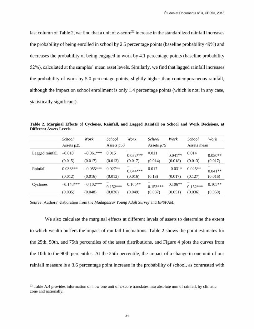
last column of Table 2, we find that a unit of z-score22 increase in the standardized rainfall increases

the probability of being enrolled in school by 2.5 percentage points (baseline probability 49%) and

decreases the probability of being engaged in work by 4.1 percentage points (baseline probability

52%), calculated at the samples’ mean asset levels. Similarly, we find that lagged rainfall increases

the probability of work by 5.0 percentage points, slightly higher than contemporaneous rainfall,

although the impact on school enrollment is only 1.4 percentage points (which is not, in any case,

statistically significant).

Table 2. Marginal Effects of Cyclones, Rainfall, and Lagged Rainfall on School and Work Decisions, at

Different Assets Levels

School Work School Work School Work School Work

Assets p25 Assets p50 Assets p75 Assets mean

Lagged rainfall –0.018 –0.061*** 0.015 –

0.052*** 0.011

–

0.041** 0.014

–

0.050** (0.015) (0.017) (0.013) (0.017) (0.014) (0.018) (0.013) (0.017)

Rainfall 0.036*** –0.055*** 0.027** –

0.044*** 0.017 –0.031* 0.025**

–

0.041** (0.012) (0.016) (0.012) (0.016) (0.13) (0.017) (0.127) (0.016)

Cyclones –0.148*** –0.102*** –

0.152*** 0.105**

–

0.153*** 0.106**

–

0.152*** 0.105**

(0.035) (0.048) (0.036) (0.049) (0.037) (0.051) (0.036) (0.050)


We also calculate the marginal effects at different levels of assets to determine the extent

to which wealth buffers the impact of rainfall fluctuations. Table 2 shows the point estimates for

the 25th, 50th, and 75th percentiles of the asset distributions, and Figure 4 plots the curves from

the 10th to the 90th percentiles. At the 25th percentile, the impact of a change in one unit of our

rainfall measure is a 3.6 percentage point increase in the probability of school, as contrasted with

22 Table A.4 provides information on how one unit of z-score translates into absolute mm of rainfall, by climatic

zone and nationally.


31

only a 1.7 percentage point increase for CMs from households at the 75th percentile (for the latter,

the effect is not statistically significant). Similarly, the change in the probability of working

associated with a one unit decline in rainfall is to raise the probability of work by 5.5 percentage

points for those belonging to the 25th percentile, while for CMs from households at the 75th

percentile, the increase in work probability is almost half that, 3.1 percentage points. As we get

further toward the lower bounds of the asset distribution, we can see that the impact of rainfall

shocks on work and school choices is much greater than that for households with greater wealth,

and conversely, the probabilities of going to school or working is less affected by climate shocks

among CMs from wealthier families (Figure 4).

Figure 4. Marginal effects of rainfall deviations on the likelihood of schooling (left panel) and working (right

panel)

Source: Authors’ elaboration based on specification (4) in Table 1.

Notes: Dashed grey curves identify the confidence intervals.

We next consider several extensions and robustness checks, reported in Table 3. First, we

include an interaction with gender (column 5). The negative and significant interaction in the work

equation suggests that young women in our cohort are even more susceptible to being pushed into

the labor market with negative rainfall deviations than male CMs. When the rains are particularly

-.02

-.01

0.0

1.0

2.0

3.0

4.0

5M

arg

inal E

ffects

of

1 u

nit c

hange in r

ain

fall

z-s

core

s

p10 p25 p50 p75 p90

percentiles on assets

-.08

-.07

-.06

-.05

-.04

-.03

-.02

-.01

0.0

1.0

2M

arg

inal E

ffects

of

1 u

nit c

hange in r

ain

fall

z-s

core

s

p10 p25 p50 p75 p90

percentiles on assets


32

favorable, however, young women experience a stronger reduction in the probability of being

engaged in a work activity.

In another specification (column 6), we exclude from the sample those individuals who

migrated from the community where they lived in 2004.23 The reason for this exclusion is that the

community variables that we introduced in the model—the presence of schools and the type of

land—are from the community where the individual lived in 2004. When migrants are excluded

from the sample, the coefficients are little changed and are of the same magnitude. Also, with such

a specification, we test whether our results are biased because of the endogeneity of migration

decisions, which are also possibly related to rainfalls. According to our results, this does not seem

the case, as our estimates are fairly robust, irrespective of the sample (with or without migrants)

that we include.

We also ran a model that excluded from the sample those CMs coming from households

who were not engaged in the agricultural sector, which we define as households where none of the

members cultivated any land between 2004 and 2011 and where neither the CMs nor their fathers

have reported that their primary sector of work is agriculture. This allows us to check whether the

rainfall effect is higher for “agricultural” households. Results, reported in column 7 of Table 3, are

stable to the exclusion of non-agricultural households. We can infer from this model that the impact

of weather shocks operates at least, in part, indirectly on schooling and work choices—for

example, affecting food prices and availability, and more generally, labor market and economic

conditions in the rural communities in which the CMs reside. Finally, in specification (8), we

estimate the model using community fixed effects. Of course, for those CMs who migrated during

23 We also estimated the baseline model on the sample of 803 individuals who never changed their residence

between 2004 and 2011. Results are stable and are available from the authors upon request.


33

our period, communities are not constant over time. Both rainfall coefficients are still significant

and of a similar magnitude.

In Table 4 we run a series of other robustness checks, by employing different definitions

of the rainfall variable. We first show, in specification (9), the results of a model using rainfall

measures based on the full year, not just the rainy season, to define the standardized rainfall

deviation. As can be seen, this change does not qualitatively change the results. Specification (10)

then reports the results based on a categorical definition of the rainfall deviation: the coefficients

are higher as rainfall deviation increases, both for schooling and work. In specification (11), we

introduce a dummy variable, instead of the rainfall deviation, to analyze more directly the specific

effect of drought.24 Results show that drought would generate a reduction in the probability of

school attendance and an increase in the probability of being engaged in work activities, especially

for the poorest CMs. Finally, specification (12) introduces a seasonality index to assess whether a

less even distribution of rainfall over the agricultural season affects the CMs’ school and work

decisions. While schooling is not affected by the intraseasonal distribution of rainfall, a higher

concentration of rainfall increases the probability of working, even though, again, assets holdings

help households mitigate such a negative effect. A higher concentration of rainfall throughout the

year is expected to negatively affect agricultural land productivity and so the revenue of

agricultural households. For this reason, according to our results, young adults may enter the

workforce to contribute to household income, even without having a large effect on schooling

participation.

24 The variable drought takes the value 1 when rainfall deviation is below the 20th percentile.


34

Table 3. Effects of Rainfall on School and Work Decisions, Robustness Checks (Sub-population and Fixed

Effects)

(2) (5) (6) (7) (8)

Equation: School

Rainfall (6 months) 0.098** 0.093** 0.082* 0.100** 0.086** (0.040) (0.043) (0.045) (0.042) (0.041)

Assets 0.010*** 0.010*** 0.008** 0.009** 0.010** (0.003) (0.003) (0.004) (0.004) (0.004)

Rainfall x Assets –0.002* –0.002* –0.000 –0.003* –0.002*

(0.001) (0.001) (0.001) (0.001) (0.001)

Woman (dummy) –0.218*** –0.219*** –0.177** –0.184***

(0.065) (0.065) (0.073) (.069)

Rainfall x Woman 0.008

(0.039)

Community fixed effects no no no no yes

Equation: Work (2) (5) (6) (7) (8)

Rainfall (6 months) –0.146*** –0.111** –0.136*** –0.133*** –0.085*

(0.047) (0.047) (0.051) (0.050) (0.046)

Assets –0.010*** –0.010*** –0.009*** –0.006* –0.007***

(0.003) (0.003) (0.003) (0.003) (0.003)

Rainfall x Assets 0.002* 0.002* 0.001 0.002 0.002

(0.001) (0.001) (0.002) (0.001) (0.001)

Woman (dummy) 0.015 0.025 0.035 0.026

(0.064) (0.057) (0.064) (0.063)

Rainfall x Woman –0.066**

(0.034)

Community fixed effects no no no no yes

Observations 8,600 8,600 7,355 7,720 8,600


Notes: For specification (2), see the notes to Table 1; (5) as in (2) plus interaction between rainfall and woman; (6) as

in (2) but by excluding migrants (see text for definition); (7) as in (2) but by excluding non-agricultural households

(see text for definition); (8) as in (2) plus community fixed effects.


35

Table 4. Effects of Rainfall on School and Working Decisions, with Different Definitions and Measures of Rainfall

Equation School Work

Specification: (2) (9) (10) (11) (12) (2) (9) (10) (11) (12)

Rainfall 0.098** 0.106*** –0.146*** –0.169***

(0.040) (0.04) (0.047) (0.049)

Assets 0.010*** 0.009*** 0.028*** 0.009*** –0.004 –0.010*** –0.009*** –0.024*** –0.009*** 0.007

(0.003) (0.003) (0.005) (0.003) (0.011) (0.003) (0.003) (0.007) (0.003) (0.008)

Rainfall x Assets –0.002* –0.003** 0.002* 0.003**

(0.001) (0.001) (0.001) (0.001)

Rainfall categories (ref: < –1)

Cat2: > –1 & < 0 0.517*** –0.479***

(0.118) (0.166)

Cat3: > 0 & < 1 0.593*** –0.530***

(0.117) (0.172)

Cat4: > 1 & < 2 0.612*** –0.790***

(0.134) (0.212)

Cat5: > 2 0.622** –0.714**

(0.250) (0.313)

Cat2 x Assets –0.018*** 0.016**

(0.005) (0.007)

Cat3 x Assets –0.021*** 0.014*

(0.006) (0.007)

Cat4 x Assets –0.015** 0.016**

(0.006) (0.008)

Cat5 x Assets –0.024*** 0.008

(0.008) (0.011)

Rainfall (over 12 months) 0.085*** –0.115***

(0.031) (0.035)

Rainfall (12 months) x Assets –0.002** 0.003***

(0.001) (0.001)

Drought –0.548*** 0.512***

(0.112) (0.169)

Drought x Assets 0.019*** –0.015**

(0.005) (0.007)

Seasonality Index (SI) –0.117 0.613***

(0.265) (0.239)

SI x Assets 0.015 –0.018**

(0.011) (0.009)

Observations 8,600 8,600 8,600 8,600 8,600 8,600 8,600 8,600 8,600 8,600

Source: Authors’ elaboration from the Madagascar Young Adult Survey and ESPAM.

Notes: For specification (2), see the note to Table 3; (9) as in (2) but with rainfall estimated over 12 months (instead of over 6 months); (10) as in (2) but

with rainfall variable defined in 5 categories (see footnote 19 for their definition) (instead of a continuous rainfall variable); (11) as in (2) but with a binary

variable identifying drought (instead of a continuous rainfall variable); (12) as in (2) plus a seasonality index and the interaction between the seasonality

index and the assets.


36

Conclusion

In this article we explore the impact of weather events on school and work decisions of a

cohort of young adults in Madagascar. This is a particularly important issue, given the

evidence that human activity is contributing to rapid climate change, which may lead to

more severe cyclones, more frequent droughts and floods, and a higher concentration of

rainfall in certain periods within a given year. Further exacerbating the potential deleterious

impacts of climate variability in poor countries, such as Madagascar, is the lack of well-

established credit and insurance markets as well as poverty that limits the ability of

households to buffer the impact of negative climate shocks.

Our focus on the impact of weather events on schooling and work is especially

pertinent to the cohort of teens and young adults we study, who are transitioning from

school to work. The concern is that deleterious shocks will cause young people to drop out

of school earlier than might be expected and enter the labor market to mitigate the impact

of drought, floods, and cyclones. A priori, the sign of the impact of rainfall deviations on

school and work is undetermined. According to the non-separable agricultural household

conceptual framework we use, while a positive increase in rainfall deviation is expected to

increase school through an income (direct) effect, the sign of the indirect (through the

rainfall-induced change in the shadow wage) effect is unknown and heavily depends on the

degree of imperfection of markets. To address this question empirically, we estimate a

bivariate probit model for a cohort of 1,119 young men and women from 2004 to 2011,

who are transitioning from their teenage years to young adulthood during that period.


37

The results of our work provide compelling evidence that negative rainfall

deviations and cyclones reduce the probability of attending school and push young men

and women into working. Most affected by these weather events are the less wealthy

households, as one would expect, given their more limited savings, less access to credit

and insurance, and generally more limited ability to cope with negative shocks. We also

find that there are both contemporaneous and lagged effects of the weather shocks, and that

they are of a similar magnitude. Another source of particular concern is our finding that

poor young women are even more susceptible to being pushed into the labor market when

negative rainfall deviations are experienced.

Our results are robust to a range of rainfall definitions. We also conduct numerous

robustness checks, including using community fixed effects and conducting individual-

level heterogeneity tests that address possible correlations between the characteristics of

the CMs and rainfall variability.

It is important to recall here that we analyze the effect of normal rainfall

variability—our period of interest is not characterized by exceptional rainfall events. The

effects we observe could be more pronounced in case of prolonged negative seasons.

The findings in our article add to a rapidly growing literature on the role of weather

shocks on a range of outcomes, including schooling and work. Although climate scientists

will continue to address the causes of weather shocks and work to prevent human activity

that contributes to climate change, our research also highlights the importance of mitigation

efforts. These are especially important for the poor in ecologically fragile countries like


38

Madagascar, which lack economic and social institutions that can help protect the

vulnerable from climate shocks.


39

Appendix: Figures and Tables

Figure A.1. Climatic zones, Köppen–Geiger climate classification system

Source: Authors’ elaboration from Kottek et al. (2006).

Notes: 1. Af. Equatorial rainforest, fully humid; 2. Am. Equatorial monsoon; 3. Aw. Equatorial savannah

with dry winter; 4. Bsh. Steppe climate (hot steppe); 5. Cfa. Warm temperate, fully humid (hot summer); 6.

Cfb. Warm temperate, fully humid (warm summer); 7. Cwa. Warm temperate, dry winter (hot summer); 8.

Cwb. Warm temperate, dry winter (warm summer).


40

Figure A.2. Cyclones having hit sample communities over the period 2004 to 2012

Source: Authors’ elaboration from the Global Risk Data Platform and Madagascar Young Adult Survey.


41

Figure A.3. Rainfall deviation from the long-term, national mean, and by climatic zones (2004–2011)

Source: Authors’ estimation.

Notes: For the definition of climatic zones, see Figure A.1.

-2-1

01

23

2004 2006 2008 2010year

national

-2-1

01

23

2004 2006 2008 2010year

zone 1

-2-1

01

23

2004 2006 2008 2010year

zone 2

-2-1

01

23

2004 2006 2008 2010year

zone 3-2

-10

12

3

2004 2006 2008 2010year

zone 4

-2-1

01

23

2004 2006 2008 2010year

zone 5

-2-1

01

23

2004 2006 2008 2010year

zone 6

-2-1

01

23

2004 2006 2008 2010year

zone 7

-2-1

01

23

2004 2006 2008 2010year

zone 8


42

Table A.1. Descriptive Statistics

Time-varying characteristics Mean

(2004)

SD

(2004)

Mean

(2011)

SD

(2011)

Age (years) 14.87 0.81 21.87 0.81

Father’s shock 7.86 0.27 18.77 0.39

Mother’s shock 5.81 0.23 12.69 0.33

Father works 91.25 0.28 81.33 0.39

Mother works 90.19 0.30 86.14 0.35

CM lives in a new household 1.34 0.16 46.47 0.50

Brothers less than 18 years old (number) 0.60 1.04 0.42 0.85

Sisters less than 18 years old (number) 0.53 0.94 0.39 0.82

Migrant 3.57 0.19 28.24 0.45

Middle school in village 71.49 0.45 77.93 0.41

High school in village 20.73 0.41 45.31 0.50

Time-invariant characteristics Mean SD

Female 51.12 0.50

Age at school entry (years) 6.95 1.82

Father has no education 50.04 0.50

Father has completed primary 17.42 0.38

Father has completed college 32.53 0.47

Mother has no education 60.50 0.49

Mother has completed primary 23.32 0.43

Mother has completed college 16.18 0.37

Household assets in 2004 (0 to 100) 20.23 16.65

Household cultivates land in 2004 40.93 0.49

Land type, coastal plain 10.44 0.30

Land type, interior plain 11.28 0.33

Land type, hill 46.97 0.49

Land type, plateau 16.03 0.36

Land type, valley 12.86 0.33

Land type, others 2.42 0.15

Paved road in village 12.69 0.33

Number of observations 1,119


Notes: If not specified differently, variables are expressed in percentages. The questionnaire asks CMs the

following question: “Did your father (your mother) have any illness or disability, or an injury during the last

seven years (since 2004), which prevented him (her) from working or carrying on business for a month or

more?” Also, we were not able to observe changes in parents’ working activities over time. In order to build

this variable, we used the answers collected in 2011–12. Working status refers to 2011–12 for those parents

who are still economically active, while it refers to the time of retirement for the inactive ones, and to the

time of death for those no longer alive.


43

Table A.2. Climatic Zones

Climatic zones 2004

(percentage)

2011

(percentage)

1. Equatorial rainforest, fully humid 15.64 16.53

2. Equatorial monsoon 19.48 17.16

3. Equatorial savannah with dry winter 13.05 14.39

4. Steppe climate (hot steppe) 4.02 4.02

5. Warm temperate, fully humid (hot summer) 7.33 7.69

6. Warm temperate, fully humid (warm summer) 20.64 18.86

7. Warm temperate, dry winter (hot summer) 11.35 10.72

8. Cwb. Warm temperate, dry winter (warm summer) 8.49 10.63

Source: Authors’ elaboration from the Madagascar Young Adult Survey.

Table A.3. Cohort Members Hit by Cyclones, in %

Year % CM hit by at least a tropical storm or

a tropical cyclone

% CM hit by at least a tropical cyclone

strength ≥ 1

2004 64.34 14.75

2005 10.99 0.09

2006 28.95 0.09

2007 27.17 2.06

2008 37.27 0.00

2009 26.18 2.23

2010 2.06 0.00

2011 4.20 0.00

Source: Authors’ elaboration from the Global Risk Data Platform and Madagascar Young Adult Survey.


44

Table A.4. Full Specification of the Base Model

Equations School Work

If CM is a girl –0.218*** 0.015

(0.065) (0.057)

Age at school entry –0.027 0.023

(0.018) (0.020)

If CM lives in a new household –0.289*** 0.089

(0.096) (0.075)

Number of child siblings, boys 0.002 –0.011

(0.028) (0.039)

Number of child siblings, girls 0.010 0.088**

(0.035) (0.037)

If father experienced any illness or death –0.184* 0.104

(0.103) (0.123)

If mother experienced any illness or death –0.125 0.294**

(0.126) (0.145)

If father works –0.129 0.046

(0.105) (0.114)

If mother works –0.026 0.293**

(0.121) (0.120)

Number of secondary schools (cycle 1) in the community 0.181** 0.011

(0.083) (0.102)

Number of secondary schools (cycle 2) in the community 0.099 –0.216*

(0.083) (0.131)

If community has access to a paved road 0.101 0.130

(0.109) (0.131)

If the hh had a land in 2004 0.149** 0.125*

(0.072) (0.068)

Rainfall deviation (6 months) 0.098** –0.146***

(0.040) (0.047)

Assets in 2004 0.010*** –0.010***

(0.003) (0.003)

Rainfall deviation x Assets –0.002* 0.002*

(0.001) (0.001)

Control for (dummies):

Age of CMs Yes Yes

Father’s education Yes Yes

Mother’s education Yes Yes

Year (2004 to 2011) Yes Yes

Climatic zone yes yes

Land type yes yes

Athrho –0.579***

(0.058)

Observations 8,600



45

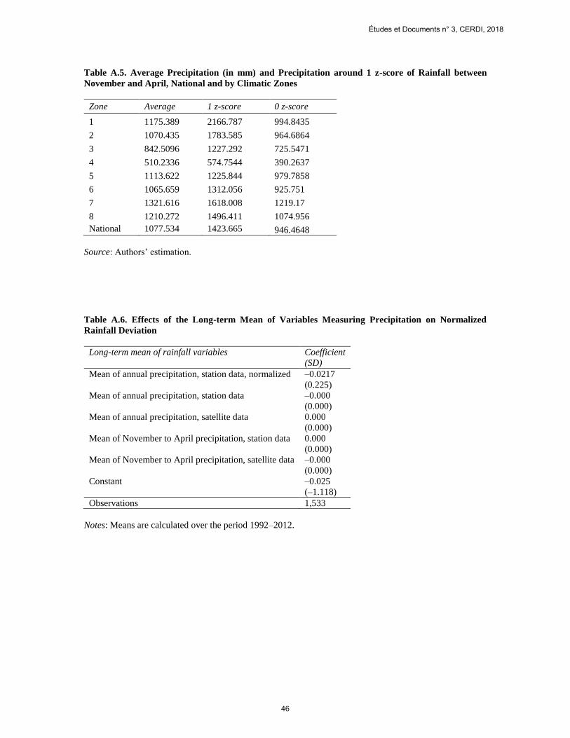
Table A.5. Average Precipitation (in mm) and Precipitation around 1 z-score of Rainfall between

November and April, National and by Climatic Zones

Zone Average 1 z-score 0 z-score

1 1175.389 2166.787 994.8435

2 1070.435 1783.585 964.6864

3 842.5096 1227.292 725.5471

4 510.2336 574.7544 390.2637

5 1113.622 1225.844 979.7858

6 1065.659 1312.056 925.751

7 1321.616 1618.008 1219.17

8 1210.272 1496.411 1074.956

National 1077.534 1423.665 946.4648


Table A.6. Effects of the Long-term Mean of Variables Measuring Precipitation on Normalized

Rainfall Deviation

Long-term mean of rainfall variables Coefficient

(SD)

Mean of annual precipitation, station data, normalized –0.0217

(0.225)

Mean of annual precipitation, station data –0.000

(0.000)

Mean of annual precipitation, satellite data 0.000

(0.000)

Mean of November to April precipitation, station data 0.000

(0.000)

Mean of November to April precipitation, satellite data –0.000

(0.000)

Constant –0.025

(–1.118)

Observations 1,533

Notes: Means are calculated over the period 1992–2012.


46

References

Asfaw, S., and G. Maggio. 2017. “Gender, Weather Shocks and Welfare: Evidence from

Malawi.” Journal of Development Studies 54 (2): 271–91.

Aubery, F., and D.E. Sahn. 2017. “Cognitive Achievement Production in Madagascar: A

Value-Added Approach.” Unpublished manuscript.

Bandyopadhyay, S., and E. Skoufias. 2015. “Rainfall Variability, Occupational Choice,

and Welfare in Rural Bangladesh.” Review of Economics of the Household 13 (3): 589–

634.

Beegle, K., R.H. Dehejia, and R. Gatti. 2006. “Child Labor and Agricultural Shocks.”

Journal of Development Economics 81 (1): 80–96.

Bengtsson, N. 2010. “How Responsive Is Body Weight to Transitory Income Changes?

Evidence from Rural Tanzania.” Journal of Development Economics 92 (1): 53–61.

Björkman-Nyqvist, M. 2013. “Income Shocks and Gender Gaps in Education: Evidence

from Uganda.” Journal of Development Economics 105: 237–53.

de Janvry, A., M. Fafchamps, and E. Sadoulet. 1991. “Peasant Household Behaviour with

Missing Markets: Some Paradoxes Explained.” Economic Journal 101 (409): 1400–

417.

de Janvry, A., and E. Sadoulet. 2006. “Progress in the Modeling of Rural Households’

Behavior under Market Failures.” In A. de Janvry and R. Kanbur, eds. Poverty,

Inequality and Development. Boston: Springer , pp. 155–81.

Dell, M., B. Jones, and B. Olken. 2014. “What Do We Learn from the Weather? The New

Climate–Economy Literature.” Journal of Economic Literature 52 (3): 740–98.


47

Dillon, A., K. McGee, and G. Oseni. 2015. “Agricultural Production, Dietary Diversity and

Climate Variability.” Journal of Development Studies 51 (8): 976–95.

Dumas, C. 2015. “Shocks and Child Labor: The Role of Markets.” FSES Working Paper,

Faculty of Economics and Social Sciences, University of Freiburg/Fribourg,

Switzerland.

FAO (Food and Agriculture Organization of the United Nations). 2016. “Welfare Impacts

of Climate Shocks: Evidence from Tanzania.” ESA Working Paper No. 16-04,

Agricultural Development Economics Division, FAO, Rome.

Filmer, D., and L.H. Pritchett. 2001. “Estimating Wealth Effects without Expenditure

Data—or Tears: An Application to Educational Enrollments in States of India.”

Demography 38 (1): 115–32.

Fitchett, J.M., and S.W. Grab. 2014. “A 66-Year Tropical Cyclone Record for South-East

Africa: Temporal Trends in a Global Context.” International Journal of Climatology

34 (13); 3604–15.

Greene, W. 2004. “The Behaviour of the Maximum Likelihood Estimator of Limited

Dependent Variable Models in the Presence of Fixed Effects.” Economic Journal 7 (1):

98–119.

Groppo, V., and K. Kraehnert. 2017. “The Impact of Extreme Weather Events on

Education.” Journal of Population Economics 30 (2): 433–72.

Henning, C.H.C.A., and A. Henningsen. 2007. “Modeling Farm Households’ Price

Responses in the Presence of Transaction Costs and Heterogeneity in Labor

Markets.”American Journal of Agricultural Economics 89 (3): 665–81.

Herrera, C., and D.E. Sahn. 2015. “The Impact of Early Childbearing on Schooling and


48

Cognitive Skills among Young Women in Madagascar.” IZA Discussion Paper No.

9362, Institute for the Study of Labor, Bonn.

Hervieu, S. 2015. “Madagascar, terminus des cyclones.” Le Monde.

http://www.lemonde.fr/planete/visuel/2015/10/10/madagascar-terminus-des-

cyclones_4786327_3244.html

Jacoby, H.G., and E. Skoufias. 1997. “Risk, Financial Markets, and Human Capital in a

Developing Country.” Review of Economic Studies 64 (3): 311–35.

Jensen, R. 2000. “Agricultural Volatility and Investments in Children.” American

Economic Review 90 (2): 399–404.

Jessoe, K., D.T. Manning, and J.E. Taylor. 2018. “Climate Change and Labour Allocation

in Rural Mexico: Evidence from Annual Fluctuations in Weather.” Economic Journal

128 (608): 230–61.

Kottek, M., J. Grieser, C. Beck, B. Rudolf, and F. Rubel. 2006. “World Map of the Köppen-

Geiger Climate Classification Updated.” Meteorologische Zeitschrift 15 (3): 259–63.

Kreft, S., D. Eckstein, L. Dorsch, and L. Fischer. 2016. “Who Suffers Most from Extreme

Weather Events? Weather-related Loss Events in 2014 and 1995 to 2014.” Global

Climate Risk Index 2016, Briefing Paper, Germanwatch e.V., Bonn.

Levine, D., and D. Yang. 2014. “The Impact of Rainfall on Rice Output in Indonesia.”

NBER Working Paper No. 20302, National Bureau of Economic Research, Cambridge,

MA.

Maccini, S., and D. Yang. 2009. “Under the Weather: Health, Schooling, and Economic

Consequences of Early-Life Rainfall.” American Economic Review 99 (3): 1006–26.

Mahajan, K., 2017. “Rainfall Shocks and the Gender Wage Gap: Evidence from Indian


49

Agriculture.” World Development 91: 156–172.

Mavume, A.F., L. Rydberg, M. Rouault, and J.R.E. Lutjeharms. 2009. “Climatology and

Landfall of Tropical Cyclones in the South-West Indian Ocean.” Western Indian Ocean

Journal of Marine Science 8(1): 15–36.

Rajaon, M.D., M.J.R. Randimbiarison, and M.M. Raherimandimby. 2015. “Les écoles

résistantes aux cyclones: Etude de cas.” Fonds d’intervention pour le développement

(FID), Madagascar. https://www.unisdr.org/2007/campaign/pdf/case-study-

madagascar-fr.pdf

Rosenzweig, M.R., and R. Evenson. 1977. “Fertility, Schooling, and the Economic

Contribution of Children of Rural India: An Econometric Analysis.” Econometrica 45

(5): 1065–79.

Sadoulet, E., and A. de Janvry. 1995. Quantitative Development Policy Analysis.

Baltimore, MD: Johns Hopkins University Press.

Sesmero, J., J. Ricker-Gilbert, and A. Cook. 2018. “How Do African Farm Households

Respond to Changes in Current and Past Weather Patterns? A Structural Panel Data

Analysis from Malawi.” American Journal of Agricultural Economics 100 (1): 115–

44.

Shah, M., and B.M. Steinberg. 2017. “Drought of Opportunities: Contemporaneous and

Long-Term Impacts of Rainfall Shocks on Human Capital.” Journal of Political

Economy 125 (2): 527–61.

Singh, I., L. Squire, and J. Strauss. 1986. Agricultural Household Models: Extensions,

Applications, and Policy. Baltimore, MD: Johns Hopkins University Press for the

World Bank.


50

Skoufias, E., S. Bandyopadhyay, and S. Olivieri. 2017. “Occupational Diversification as

an Adaptation to Rainfall Variability in Rural India.” Agricultural Economics 48 (1):

77–89.

Tiberti, L., and M. Tiberti. 2015. “Rural Policies, Price Change and Poverty in Tanzania:

An Agricultural Household Model-Based Assessment.” Journal of African Economies

24 (2): 193–229.

Tiwari, S., H.G. Jacoby, and E. Skoufias. 2017. “Monsoon Babies: Rainfall Shocks and

Child Nutrition in Nepal.” Economic Development and Cultural Change 65 (2): 167–

88.

UNICEF (United Nations Children’s Fund). 2016. “Madagascar El Niño Drought

Humanitarian Situation Report.” September 2016, UNICEF–Madagascar.

https://reliefweb.int/sites/reliefweb.int/files/resources/UNICEF%20Madagascar%20H

umanitarian%20SitRep%20-%20Sep%202016.pdf

Villalobos, L. 2016. “Effects of Weather on Daily School Attendance Decisions and

Academic Performance in Rural Costa Rica.” Unpublished manuscript, Department of

Economics, University of Gothenburg.

Walsh, R.P.D., and D. M. Lawler. 1981. “Rainfall Seasonality: Description, Spatial

Patterns and Change Through Time.” Weather 36 (7): 201–8.


51

SÉRIE ÉTUDES ET DOCUMENTS

Documents

Transcript of SÉRIE ÉTUDES ET DOCUMENTS