SRI VIDYA COLLEGE OF ENGINEERING AND TECHNOLOGY...
42
SRI VIDYA COLLEGE OF ENGINEERING AND TECHNOLOGY COURSE MATERIAL (LECTURE NOTES) CS6704 RMT UNIT -1 Page 1 Concept and Definition Operations research signifies research on operations. It is the organized application of modern science, mathematics and computer techniques to complex military, government, business or industrial problems arising in the direction and management of large systems of men, material, money and machines. The purpose is to provide the management with explicit quantitative understanding and assessment of complex situations to have sound basics for arriving at best decisions. Operations research seeks the optimum state in all conditions and thus provides optimum solution to organizational problems. Definition: OR is a scientific methodology – analytical, experimental and quantitative – which by assessing the overall implications of various alternative courses of action in a management system provides an improved basis for management decisions. Characteristics of OR (Features) The essential characteristics of OR are 1. Inter-disciplinary team approach – The optimum solution is found by a team of scientists selected from various disciplines. 2. Wholistic approach to the system – OR takes into account all significant factors and finds the best optimum solution to the total organization. 3. Imperfectness of solutions – Improves the quality of solution. 4. Use of scientific research – Uses scientific research to reach optimum solution. 5. To optimize the total output – It tries to optimize by maximizing the profit and minimizing the loss. Phases of OR OR study generally involves the following major phases 1. Defining the problem and gathering data 2. Formulating a mathematical model 3. Deriving solutions from the model www.studentsfocus.com
Transcript of SRI VIDYA COLLEGE OF ENGINEERING AND TECHNOLOGY...
SRI VIDYA COLLEGE OF ENGINEERING AND TECHNOLOGY COURSE MATERIAL (LECTURE NOTES)
CS6704 RMT UNIT -1 Page 1
Concept and Definition Operations research signifies research on operations. It is the organized application of modern
science, mathematics and computer techniques to complex military, government, business or
industrial problems arising in the direction and management of large systems of men, material,
money and machines. The purpose is to provide the management with explicit quantitative
understanding and assessment of complex situations to have sound basics for arriving at best
decisions.
Operations research seeks the optimum state in all conditions and thus provides optimum
solution to organizational problems.
Definition: OR is a scientific methodology – analytical, experimental and quantitative – which
by assessing the overall implications of various alternative courses of action in a management
system provides an improved basis for management decisions.
Characteristics of OR (Features) The essential characteristics of OR are
1. Inter-disciplinary team approach – The optimum solution is found by a team of
scientists selected from various disciplines.
2. Wholistic approach to the system – OR takes into account all significant factors and
finds the best optimum solution to the total organization.
3. Imperfectness of solutions – Improves the quality of solution.
4. Use of scientific research – Uses scientific research to reach optimum solution.
5. To optimize the total output – It tries to optimize by maximizing the profit and
minimizing the loss.
Phases of OR OR study generally involves the following major phases
1. Defining the problem and gathering data
2. Formulating a mathematical model
3. Deriving solutions from the model
www.studentsfocus.com
SRI VIDYA COLLEGE OF ENGINEERING AND TECHNOLOGY COURSE MATERIAL (LECTURE NOTES)
CS6704 RMT UNIT -1 Page 2
4. Testing the model and its solutions
5. Preparing to apply the model
6. Implementation
1. Defining the problem and gathering data
x The first task is to study the relevant system and develop a well-defined statement of the
problem. This includes determining appropriate objectives, constraints, interrelationships
and alternative course of action.
x The OR team normally works in an advisory capacity. The team performs a detailed
technical analysis of the problem and then presents recommendations to the management.
x Ascertaining the appropriate objectives is very important aspect of problem definition.
Some of the objectives include maintaining stable price, profits, increasing the share in
market, improving work morale etc.
x OR team typically spends huge amount of time in gathering relevant data.
o To gain accurate understanding of problem
o To provide input for next phase.
x OR teams uses Data mining methods to search large databases for interesting patterns
that may lead to useful decisions.
2. Formulating a mathematical model This phase is to reformulate the problem in terms of mathematical symbols and expressions. The
mathematical model of a business problem is described as the system of equations and related
mathematical expressions. Thus
1. Decision variables (x1, x2 … xn) – ‘n’ related quantifiable decisions to be made.
2. Objective function – measure of performance (profit) expressed as mathematical
function of decision variables. For example P=3x1 +5x2 + … + 4xn
3. Constraints – any restriction on values that can be assigned to decision variables in
terms of inequalities or equations. For example x1 +2x2 ≥ 20
4. Parameters – the constant in the constraints (right hand side values)
www.studentsfocus.com
SRI VIDYA COLLEGE OF ENGINEERING AND TECHNOLOGY COURSE MATERIAL (LECTURE NOTES)
CS6704 RMT UNIT -1 Page 3
Principles of Modeling The model building and their uses both should be consciously aware of the following ten
principles
1. Do not build up a complicated model when simple one will suffice
2. Beware of molding the problem to fit the technique
3. The deduction phase of modeling must be conducted rigorously
4. Models should be validated prior to implementation
5. A model should never be taken too literally
6. A model should neither be pressed to do nor criticized for failing to do that for which it
was never intended
7. Beware of over-selling a model
8. Some of the primary benefits of modeling are associated with the process of developing
the model
9. A model cannot be any better than the information that goes into it
10. Models cannot replace decision makers
Simplifications of OR Models While constructing a model, two conflicting objectives usually strike in our mind
1. The model should be as accurate as possible
2. It should be as easy as possible in solving
Besides, the management must be able to understand the solution of the model and must be
capable of using it. So the reality of the problem under study should be simplified to the extent
when there is no loss of accuracy. The model can be simplified by
x Omitting certain variable
x Changing the nature of variables
x Aggregating the variables
x Changing the relationship between variables
Modifying the constraints, etc
www.studentsfocus.com
SRI VIDYA COLLEGE OF ENGINEERING AND TECHNOLOGY COURSE MATERIAL (LECTURE NOTES)
CS6704 RMT UNIT -1 Page 4
Introduction to Linear Programming A linear form is meant a mathematical expression of the type a1x1 + a2x2 + …. + anxn, where a1,
a2, …, an are constants and x1, x2 … xn are variables. The term Programming refers to the process
of determining a particular program or plan of action. So Linear Programming (LP) is one of the
most important optimization (maximization / minimization) techniques developed in the field of
Operations Research (OR).
The methods applied for solving a linear programming problem are basically simple problems; a
solution can be obtained by a set of simultaneous equations. However a unique solution for a set
of simultaneous equations in n-variables (x1, x2 … xn), at least one of them is non-zero, can be
obtained if there are exactly n relations. When the number of relations is greater than or less than
n, a unique solution does not exist but a number of trial solutions can be found.
In various practical situations, the problems are seen in which the number of relations is not
equal to the number of the number of variables and many of the relations are in the form of
inequalities (≤ or ≥) to maximize or minimize a linear function of the variables subject to such
conditions. Such problems are known as Linear Programming Problem (LPP).
Definition – The general LPP calls for optimizing (maximizing / minimizing) a linear function
of variables called the ‘Objective function’ subject to a set of linear equations and / or
inequalities called the ‘Constraints’ or ‘Restrictions’.
General form of LPP We formulate a mathematical model for general problem of allocating resources to activities. In
particular, this model is to select the values for x1, x2 … xn so as to maximize or minimize
Z = c1x1 + c2x2 +………….+cnxn
subject to restrictions
a11x1 + a12x2 + …..........+a1nxn (≤ or ≥) b1
a21x1 + a22x2 + ………..+a2nxn (≤ or ≥) b2
.
www.studentsfocus.com

SRI VIDYA COLLEGE OF ENGINEERING AND TECHNOLOGY COURSE MATERIAL (LECTURE NOTES)
CS6704 RMT UNIT -1 Page 5
.
. am1x1 + am2x2 + ……….+amnxn (≤ or ≥) bm
and x1 ≥ 0, x2 ≥ 0,…, xn ≥ 0
Where
Z = value of overall measure of performance
xj = level of activity (for j = 1, 2, ..., n)
cj = increase in Z that would result from each unit increase in level of activity j
bi = amount of resource i that is available for allocation to activities (for i = 1,2, …, m)
aij = amount of resource i consumed by each unit of activity j
Resource
Resource usage per unit of activity Amount of resource
available Activity
1 2 …………………….. n
1
2
.
.
.
m
a11 a12 …………………….a1n
a21 a22 …………………….a2n
.
.
.
am1 am2 …………………….amn
b1
b2
.
.
.
bm
Contribution to Z
per unit of activity c1 c2 ………………………..cn
Data needed for LP model
x The level of activities x1, x2………xn are called decision variables.
x The values of the cj, bi, aij (for i=1, 2 … m and j=1, 2 … n) are the input constants for the
model. They are called as parameters of the model.
x The function being maximized or minimized Z = c1x1 + c2x2 +…. +cnxn is called
objective function.
x The restrictions are normally called as constraints. The constraint ai1x1 + ai2x2 … ainxn
are sometimes called as functional constraint (L.H.S constraint). xj ≥ 0 restrictions are
called non-negativity constraint.
www.studentsfocus.com
SRI VIDYA COLLEGE OF ENGINEERING AND TECHNOLOGY COURSE MATERIAL (LECTURE NOTES)
CS6704 RMT UNIT -1 Page 6
Advantages of Linear Programming Techniques 1. It helps us in making the optimum utilization of productive resources.
2. The quality of decisions may also be improved by linear programming techniques.
3. Provides practically solutions.
4. In production processes, high lighting of bottlenecks is the most significant advantage of
this technique.
Limitations of Linear Programming Some limitations are associated with linear programming techniques
1. In some problems, objective functions and constraints are not linear. Generally, in real
life situations concerning business and industrial problems constraints are not linearly
treated to variables.
2. There is no guarantee of getting integer valued solutions. For example, in finding out how
many men and machines would be required to perform a particular job, rounding off the
solution to the nearest integer will not give an optimal solution. Integer programming
deals with such problems.
3. Linear programming model does not take into consideration the effect of time and
uncertainty. Thus the model should be defined in such a way that any change due to
internal as well as external factors can be incorporated.
4. Sometimes large scale problems cannot be solved with linear programming techniques
even when the computer facility is available. Such difficulty may be removed by
decomposing the main problem into several small problems and then solving them
separately.
5. Parameters appearing in the model are assumed to be constant. But, in real life situations
they are neither constant nor deterministic.
6. Linear programming deals with only single objective, whereas in real life situation
problems come across with multi objectives. Goal programming and multi-objective
programming deals with such problems.
www.studentsfocus.com
SRI VIDYA COLLEGE OF ENGINEERING AND TECHNOLOGY COURSE MATERIAL (LECTURE NOTES)
CS6704 RMT UNIT -1 Page 7
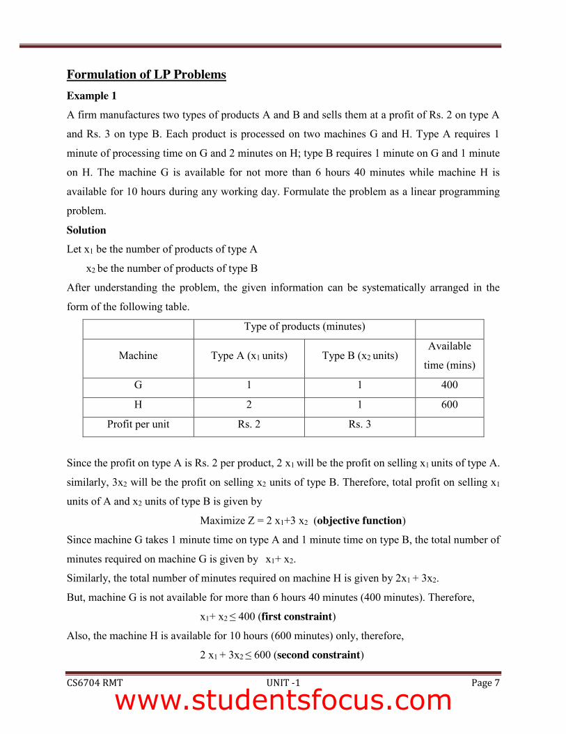
Formulation of LP Problems Example 1 A firm manufactures two types of products A and B and sells them at a profit of Rs. 2 on type A
and Rs. 3 on type B. Each product is processed on two machines G and H. Type A requires 1
minute of processing time on G and 2 minutes on H; type B requires 1 minute on G and 1 minute
on H. The machine G is available for not more than 6 hours 40 minutes while machine H is
available for 10 hours during any working day. Formulate the problem as a linear programming
problem.
Solution Let x1 be the number of products of type A
x2 be the number of products of type B
After understanding the problem, the given information can be systematically arranged in the
form of the following table.
Type of products (minutes)
Machine Type A (x1 units) Type B (x2 units) Available
time (mins)
G 1 1 400
H 2 1 600
Profit per unit Rs. 2 Rs. 3
Since the profit on type A is Rs. 2 per product, 2 x1 will be the profit on selling x1 units of type A.
similarly, 3x2 will be the profit on selling x2 units of type B. Therefore, total profit on selling x1
units of A and x2 units of type B is given by
Maximize Z = 2 x1+3 x2 (objective function)
Since machine G takes 1 minute time on type A and 1 minute time on type B, the total number of
minutes required on machine G is given by x1+ x2.
Similarly, the total number of minutes required on machine H is given by 2x1 + 3x2.
But, machine G is not available for more than 6 hours 40 minutes (400 minutes). Therefore,
x1+ x2 ≤ 400 (first constraint) Also, the machine H is available for 10 hours (600 minutes) only, therefore,
2 x1 + 3x2 ≤ 600 (second constraint)
www.studentsfocus.com
SRI VIDYA COLLEGE OF ENGINEERING AND TECHNOLOGY COURSE MATERIAL (LECTURE NOTES)
CS6704 RMT UNIT -1 Page 8
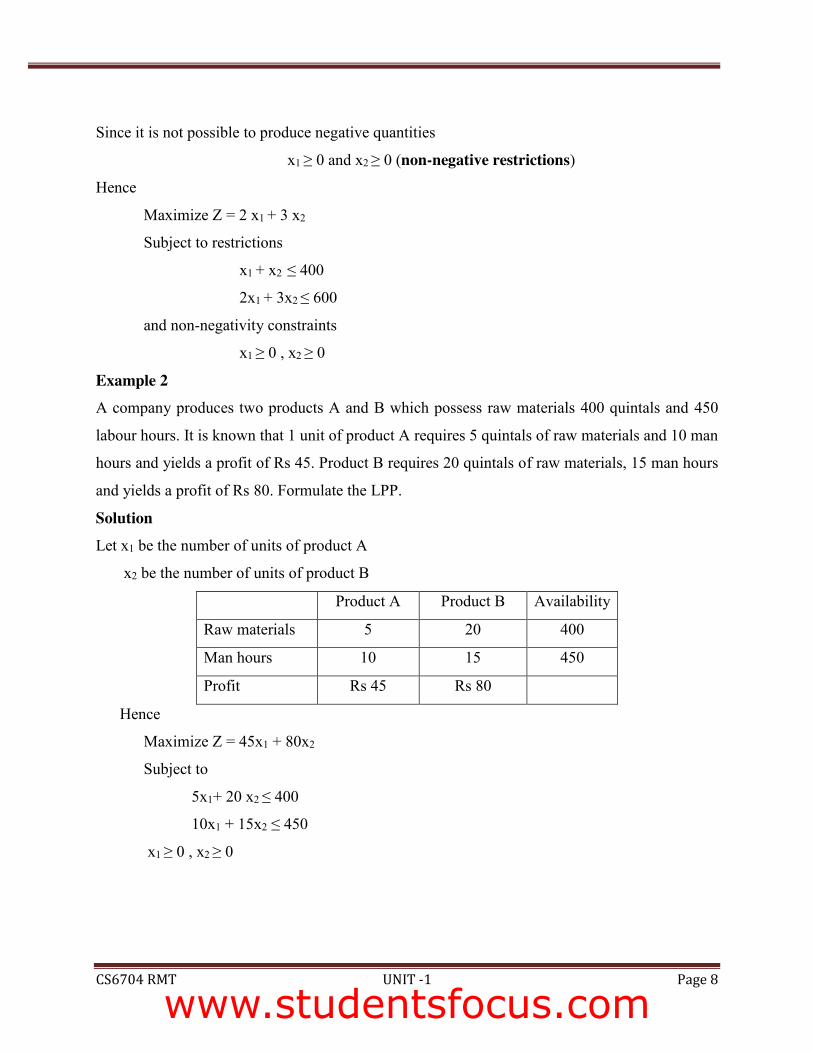
Since it is not possible to produce negative quantities
x1 ≥ 0 and x2 ≥ 0 (non-negative restrictions)
Hence
Maximize Z = 2 x1 + 3 x2
Subject to restrictions
x1 + x2 ≤ 400
2x1 + 3x2 ≤ 600
and non-negativity constraints
x1 ≥ 0 , x2 ≥ 0
Example 2
A company produces two products A and B which possess raw materials 400 quintals and 450
labour hours. It is known that 1 unit of product A requires 5 quintals of raw materials and 10 man
hours and yields a profit of Rs 45. Product B requires 20 quintals of raw materials, 15 man hours
and yields a profit of Rs 80. Formulate the LPP.
Solution Let x1 be the number of units of product A
x2 be the number of units of product B
Product A Product B Availability
Raw materials 5 20 400
Man hours 10 15 450
Profit Rs 45 Rs 80
Hence
Maximize Z = 45x1 + 80x2
Subject to
5x1+ 20 x2 ≤ 400
10x1 + 15x2 ≤ 450
x1 ≥ 0 , x2 ≥ 0
www.studentsfocus.com
SRI VIDYA COLLEGE OF ENGINEERING AND TECHNOLOGY COURSE MATERIAL (LECTURE NOTES)
CS6704 RMT UNIT -1 Page 9
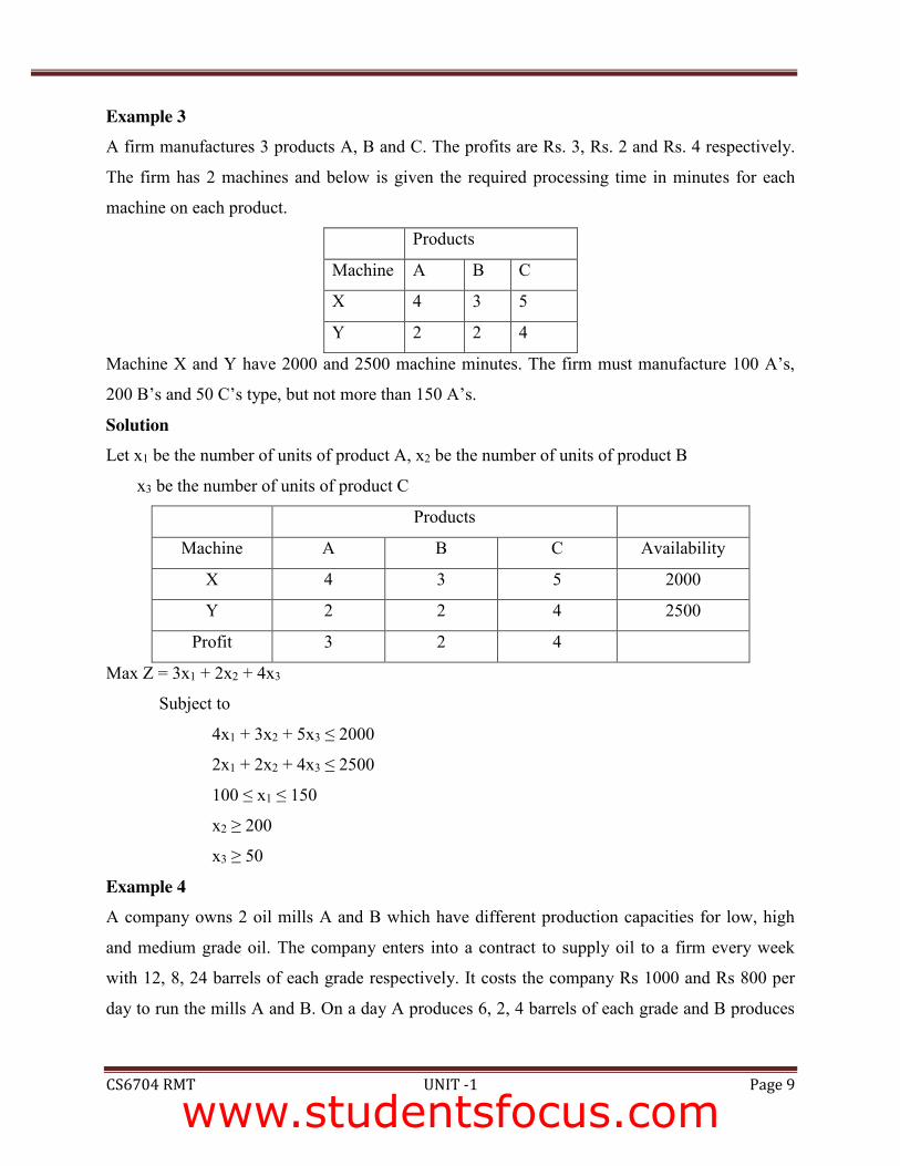
Example 3 A firm manufactures 3 products A, B and C. The profits are Rs. 3, Rs. 2 and Rs. 4 respectively.
The firm has 2 machines and below is given the required processing time in minutes for each
machine on each product.
Products
Machine A B C
X 4 3 5
Y 2 2 4
Machine X and Y have 2000 and 2500 machine minutes. The firm must manufacture 100 A’s,
200 B’s and 50 C’s type, but not more than 150 A’s.
Solution Let x1 be the number of units of product A, x2 be the number of units of product B
x3 be the number of units of product C
Products
Machine A B C Availability
X 4 3 5 2000
Y 2 2 4 2500
Profit 3 2 4
Max Z = 3x1 + 2x2 + 4x3
Subject to
4x1 + 3x2 + 5x3 ≤ 2000
2x1 + 2x2 + 4x3 ≤ 2500
100 ≤ x1 ≤ 150
x2 ≥ 200
x3 ≥ 50
Example 4 A company owns 2 oil mills A and B which have different production capacities for low, high
and medium grade oil. The company enters into a contract to supply oil to a firm every week
with 12, 8, 24 barrels of each grade respectively. It costs the company Rs 1000 and Rs 800 per
day to run the mills A and B. On a day A produces 6, 2, 4 barrels of each grade and B produces
www.studentsfocus.com
SRI VIDYA COLLEGE OF ENGINEERING AND TECHNOLOGY COURSE MATERIAL (LECTURE NOTES)
CS6704 RMT UNIT -1 Page 10
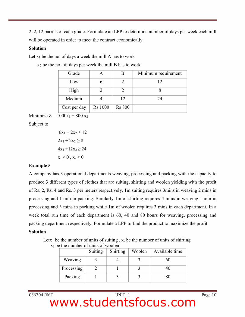
2, 2, 12 barrels of each grade. Formulate an LPP to determine number of days per week each mill
will be operated in order to meet the contract economically.
Solution Let x1 be the no. of days a week the mill A has to work
x2 be the no. of days per week the mill B has to work
Grade A B Minimum requirement
Low 6 2 12
High 2 2 8
Medium 4 12 24
Cost per day Rs 1000 Rs 800
Minimize Z = 1000x1 + 800 x2
Subject to
6x1 + 2x2 ≥ 12
2x1 + 2x2 ≥ 8
4x1 +12x2 ≥ 24
x1 ≥ 0 , x2 ≥ 0
Example 5 A company has 3 operational departments weaving, processing and packing with the capacity to
produce 3 different types of clothes that are suiting, shirting and woolen yielding with the profit
of Rs. 2, Rs. 4 and Rs. 3 per meters respectively. 1m suiting requires 3mins in weaving 2 mins in
processing and 1 min in packing. Similarly 1m of shirting requires 4 mins in weaving 1 min in
processing and 3 mins in packing while 1m of woolen requires 3 mins in each department. In a
week total run time of each department is 60, 40 and 80 hours for weaving, processing and
packing department respectively. Formulate a LPP to find the product to maximize the profit.
Solution Letx1 be the number of units of suiting , x2 be the number of units of shirting
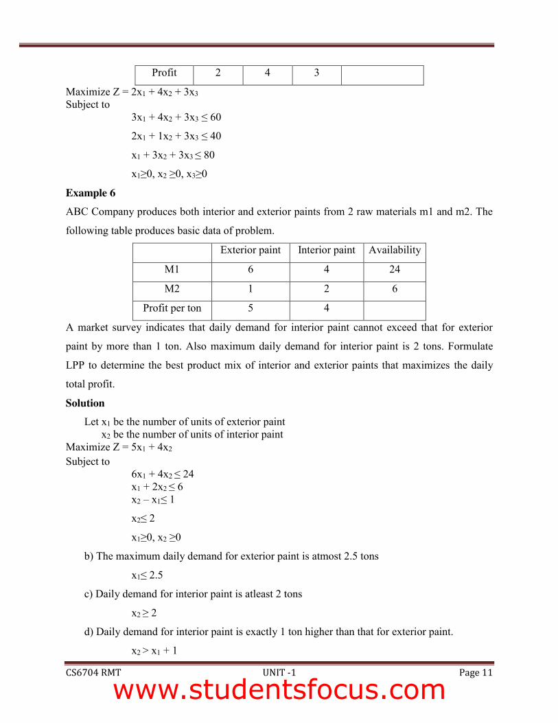
x3 be the number of units of woolen Suiting Shirting Woolen Available time
Weaving 3 4 3 60
Processing 2 1 3 40
Packing 1 3 3 80
www.studentsfocus.com
SRI VIDYA COLLEGE OF ENGINEERING AND TECHNOLOGY COURSE MATERIAL (LECTURE NOTES)
CS6704 RMT UNIT -1 Page 11
Profit 2 4 3
Maximize Z = 2x1 + 4x2 + 3x3 Subject to
3x1 + 4x2 + 3x3 ≤ 60
2x1 + 1x2 + 3x3 ≤ 40
x1 + 3x2 + 3x3 ≤ 80
x1≥0, x2 ≥0, x3≥0
Example 6 ABC Company produces both interior and exterior paints from 2 raw materials m1 and m2. The
following table produces basic data of problem.
Exterior paint Interior paint Availability
M1 6 4 24
M2 1 2 6
Profit per ton 5 4
A market survey indicates that daily demand for interior paint cannot exceed that for exterior
paint by more than 1 ton. Also maximum daily demand for interior paint is 2 tons. Formulate
LPP to determine the best product mix of interior and exterior paints that maximizes the daily
total profit.
Solution Let x1 be the number of units of exterior paint x2 be the number of units of interior paint
Maximize Z = 5x1 + 4x2 Subject to
6x1 + 4x2 ≤ 24 x1 + 2x2 ≤ 6 x2 – x1≤ 1
x2≤ 2
x1≥0, x2 ≥0
b) The maximum daily demand for exterior paint is atmost 2.5 tons
x1≤ 2.5
c) Daily demand for interior paint is atleast 2 tons
x2 ≥ 2
d) Daily demand for interior paint is exactly 1 ton higher than that for exterior paint.
x2 > x1 + 1
www.studentsfocus.com
SRI VIDYA COLLEGE OF ENGINEERING AND TECHNOLOGY COURSE MATERIAL (LECTURE NOTES)
CS6704 RMT UNIT -1 Page 12
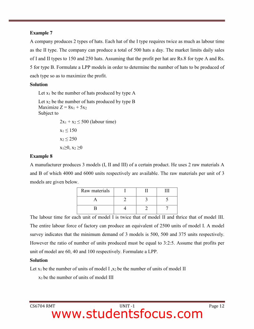
Example 7 A company produces 2 types of hats. Each hat of the I type requires twice as much as labour time
as the II type. The company can produce a total of 500 hats a day. The market limits daily sales
of I and II types to 150 and 250 hats. Assuming that the profit per hat are Rs.8 for type A and Rs.
5 for type B. Formulate a LPP models in order to determine the number of hats to be produced of
each type so as to maximize the profit.
Solution Let x1 be the number of hats produced by type A
Let x2 be the number of hats produced by type B Maximize Z = 8x1 + 5x2 Subject to
2x1 + x2 ≤ 500 (labour time)
x1 ≤ 150
x2 ≤ 250
x1≥0, x2 ≥0
Example 8 A manufacturer produces 3 models (I, II and III) of a certain product. He uses 2 raw materials A
and B of which 4000 and 6000 units respectively are available. The raw materials per unit of 3
models are given below.
Raw materials I II III
A 2 3 5
B 4 2 7
The labour time for each unit of model I is twice that of model II and thrice that of model III.
The entire labour force of factory can produce an equivalent of 2500 units of model I. A model
survey indicates that the minimum demand of 3 models is 500, 500 and 375 units respectively.
However the ratio of number of units produced must be equal to 3:2:5. Assume that profits per
unit of model are 60, 40 and 100 respectively. Formulate a LPP.
Solution Let x1 be the number of units of model I ,x2 be the number of units of model II
x3 be the number of units of model III
www.studentsfocus.com
SRI VIDYA COLLEGE OF ENGINEERING AND TECHNOLOGY COURSE MATERIAL (LECTURE NOTES)
CS6704 RMT UNIT -1 Page 13
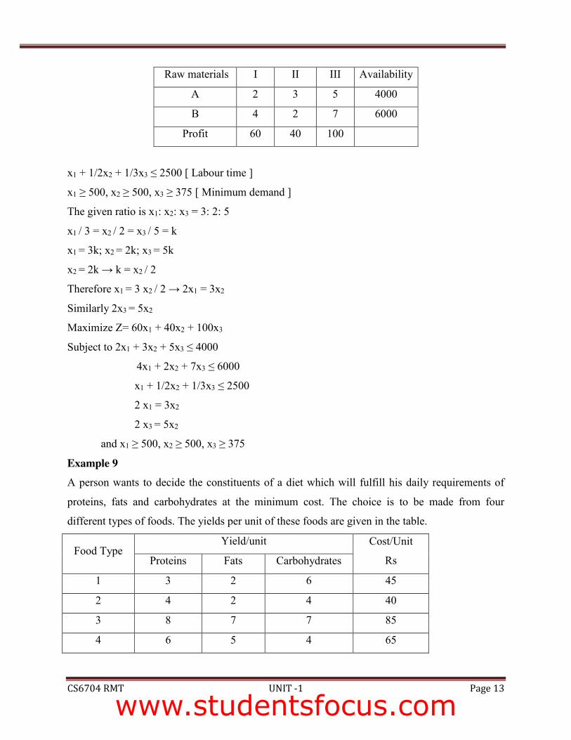
Raw materials I II III Availability
A 2 3 5 4000
B 4 2 7 6000
Profit 60 40 100
x1 + 1/2x2 + 1/3x3 ≤ 2500 [ Labour time ]
x1 ≥ 500, x2 ≥ 500, x3 ≥ 375 [ Minimum demand ]
The given ratio is x1: x2: x3 = 3: 2: 5
x1 / 3 = x2 / 2 = x3 / 5 = k
x1 = 3k; x2 = 2k; x3 = 5k
x2 = 2k → k = x2 / 2
Therefore x1 = 3 x2 / 2 → 2x1 = 3x2
Similarly 2x3 = 5x2
Maximize Z= 60x1 + 40x2 + 100x3
Subject to 2x1 + 3x2 + 5x3 ≤ 4000
4x1 + 2x2 + 7x3 ≤ 6000
x1 + 1/2x2 + 1/3x3 ≤ 2500
2 x1 = 3x2
2 x3 = 5x2
and x1 ≥ 500, x2 ≥ 500, x3 ≥ 375
Example 9 A person wants to decide the constituents of a diet which will fulfill his daily requirements of
proteins, fats and carbohydrates at the minimum cost. The choice is to be made from four
different types of foods. The yields per unit of these foods are given in the table.
Food Type Yield/unit Cost/Unit
Rs Proteins Fats Carbohydrates
1 3 2 6 45
2 4 2 4 40
3 8 7 7 85
4 6 5 4 65
www.studentsfocus.com
SRI VIDYA COLLEGE OF ENGINEERING AND TECHNOLOGY COURSE MATERIAL (LECTURE NOTES)
CS6704 RMT UNIT -1 Page 14
Minimum
Requirement 800 200 700
Formulate the LP for the problem.
Solution Let x1 be the number of units of food type l , x2 be the number of units of food type 2
x3 be the number of units of food type 3, x4 be the number of units of food type 4
Minimize Z = 45x1 + 40x2 + 85x3 + 65x4 Subject to
3x1 + 4x2 + 8x3 + 6x4 ≥ 800
2x1 + 2x2 + 7x3 + 5x4 ≥ 200
6x1 + 4x2 + 7x3 + 4x4 ≥ 700
x1≥0, x2 ≥0, x3≥0, x4≥0
Graphical Solution Procedure The graphical solution procedure
1. Consider each inequality constraint as equation.
2. Plot each equation on the graph as each one will geometrically represent a straight line.
3. Shade the feasible region. Every point on the line will satisfy the equation of the line. If
the inequality constraint corresponding to that line is ‘≤’ then the region below the line
lying in the first quadrant is shaded. Similarly for ‘≥’ the region above the line is shaded.
The points lying in the common region will satisfy the constraints. This common region
is called feasible region. 4. Choose the convenient value of Z and plot the objective function line.
5. Pull the objective function line until the extreme points of feasible region.
a. In the maximization case this line will stop far from the origin and passing
through at least one corner of the feasible region.
b. In the minimization case, this line will stop near to the origin and passing through
at least one corner of the feasible region.
6. Read the co-ordinates of the extreme points selected in step 5 and find the maximum or
minimum value of Z.
www.studentsfocus.com

SRI VIDYA COLLEGE OF ENGINEERING AND TECHNOLOGY COURSE MATERIAL (LECTURE NOTES)
CS6704 RMT UNIT -1 Page 15
Definitions
1. Solution – Any specification of the values for decision variable among (x1, x2… xn) is
called a solution.
2. Feasible solution is a solution for which all constraints are satisfied.
3. Infeasible solution is a solution for which atleast one constraint is not satisfied.
4. Feasible region is a collection of all feasible solutions.
5. Optimal solution is a feasible solution that has the most favorable value of the objective
function.
6. Most favorable value is the largest value if the objective function is to be maximized,
whereas it is the smallest value if the objective function is to be minimized.
7. Multiple optimal solution – More than one solution with the same optimal value of the
objective function.
8. Unbounded solution – If the value of the objective function can be increased or
decreased indefinitely such solutions are called unbounded solution.
9. Feasible region – The region containing all the solutions of an inequality
10. Corner point feasible solution is a solution that lies at the corner of the feasible region.
Example problems
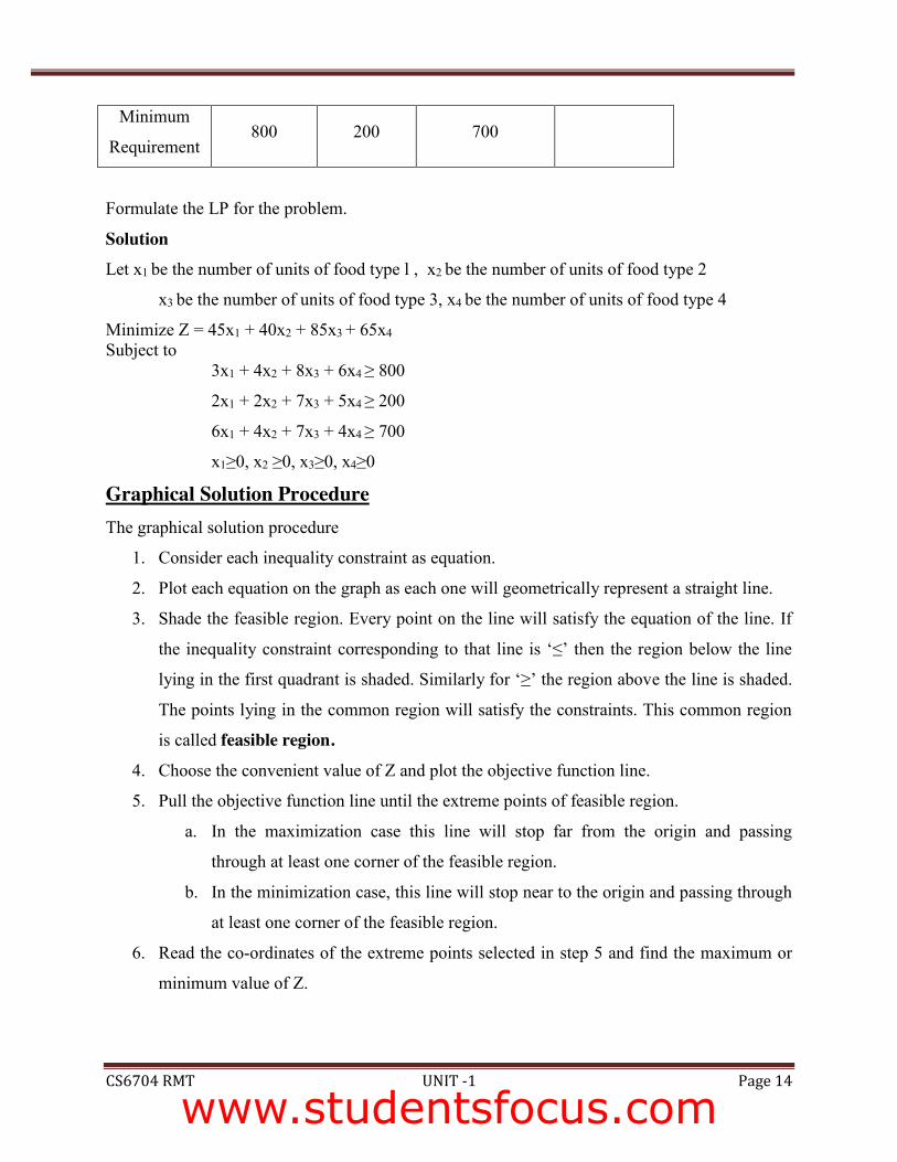
Example 1 Solve 3x + 5y < 15 graphically
Solution Write the given constraint in the form of equation i.e. 3x + 5y = 15
Put x=0 then the value y=3
Put y=0 then the value x=5
Therefore the coordinates are (0, 3) and (5, 0). Thus these points are joined to form a straight line
as shown in the graph.
Put x=0, y=0 in the given constraint then
0<15, the condition is true. (0, 0) is solution nearer to origin. So shade the region below the line,
which is the feasible region.
www.studentsfocus.com
SRI VIDYA COLLEGE OF ENGINEERING AND TECHNOLOGY COURSE MATERIAL (LECTURE NOTES)
CS6704 RMT UNIT -1 Page 16
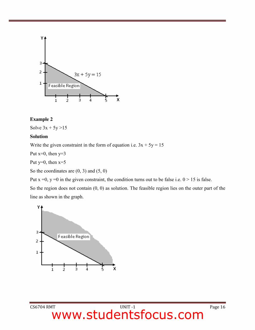
Example 2 Solve 3x + 5y >15
Solution Write the given constraint in the form of equation i.e. 3x + 5y = 15
Put x=0, then y=3
Put y=0, then x=5
So the coordinates are (0, 3) and (5, 0)
Put x =0, y =0 in the given constraint, the condition turns out to be false i.e. 0 > 15 is false.
So the region does not contain (0, 0) as solution. The feasible region lies on the outer part of the
line as shown in the graph.
www.studentsfocus.com
SRI VIDYA COLLEGE OF ENGINEERING AND TECHNOLOGY COURSE MATERIAL (LECTURE NOTES)
CS6704 RMT UNIT -1 Page 17
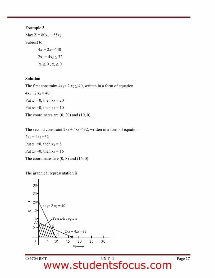
Example 3 Max Z = 80x1 + 55x2
Subject to
4x1+ 2x2 ≤ 40
2x1 + 4x2 ≤ 32
x1 ≥ 0 , x2 ≥ 0
Solution The first constraint 4x1+ 2 x2 ≤ 40, written in a form of equation
4x1+ 2 x2 = 40
Put x1 =0, then x2 = 20
Put x2 =0, then x1 = 10
The coordinates are (0, 20) and (10, 0)
The second constraint 2x1 + 4x2 ≤ 32, written in a form of equation
2x1 + 4x2 =32
Put x1 =0, then x2 = 8
Put x2 =0, then x1 = 16
The coordinates are (0, 8) and (16, 0)
The graphical representation is
www.studentsfocus.com
SRI VIDYA COLLEGE OF ENGINEERING AND TECHNOLOGY COURSE MATERIAL (LECTURE NOTES)
CS6704 RMT UNIT -1 Page 18
The corner points of feasible region are A, B and C. So the coordinates for the corner points are
A (0, 8)
B (8, 4) (Solve the two equations 4x1+ 2 x2 = 40 and 2x1 + 4x2 =32 to get the coordinates)
C (10, 0)
We know that Max Z = 80x1 + 55x2
At A (0, 8)
Z = 80(0) + 55(8) = 440
At B (8, 4)
Z = 80(8) + 55(4) = 860
At C (10, 0)
Z = 80(10) + 55(0) = 800
The maximum value is obtained at the point B. Therefore Max Z = 860 and x1 = 8, x2 = 4
Example 4 Minimize Z = 10x1 + 4x2
Subject to
3x1 + 2x2 ≥ 60
7x1 + 2x2 ≥ 84
3x1 +6x2 ≥ 72
x1 ≥ 0 , x2 ≥ 0
Solution The first constraint 3x1 + 2x2 ≥ 60, written in a form of equation
3x1 + 2x2 = 60
Put x1 =0, then x2 = 30
Put x2 =0, then x1 = 20
www.studentsfocus.com
SRI VIDYA COLLEGE OF ENGINEERING AND TECHNOLOGY COURSE MATERIAL (LECTURE NOTES)
CS6704 RMT UNIT -1 Page 19
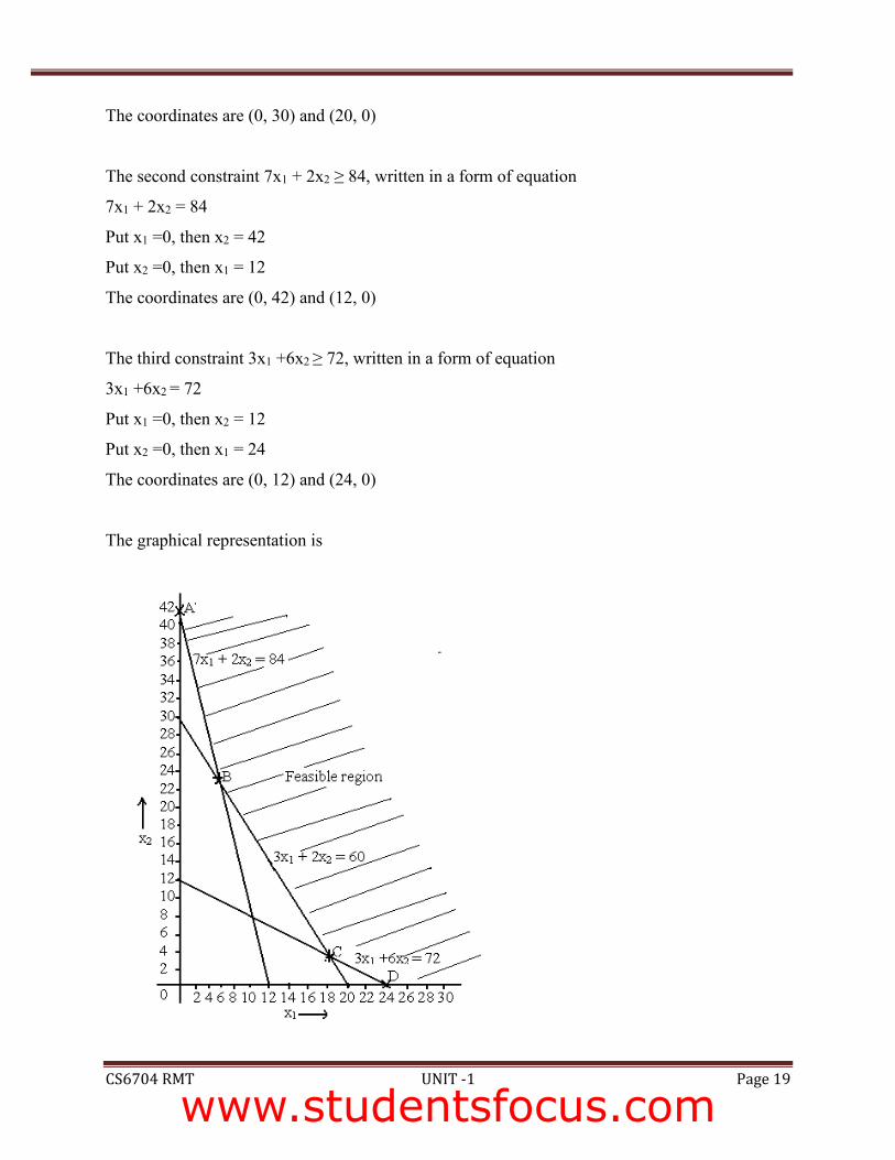
The coordinates are (0, 30) and (20, 0)
The second constraint 7x1 + 2x2 ≥ 84, written in a form of equation
7x1 + 2x2 = 84
Put x1 =0, then x2 = 42
Put x2 =0, then x1 = 12
The coordinates are (0, 42) and (12, 0)
The third constraint 3x1 +6x2 ≥ 72, written in a form of equation
3x1 +6x2 = 72
Put x1 =0, then x2 = 12
Put x2 =0, then x1 = 24
The coordinates are (0, 12) and (24, 0)
The graphical representation is
www.studentsfocus.com
SRI VIDYA COLLEGE OF ENGINEERING AND TECHNOLOGY COURSE MATERIAL (LECTURE NOTES)
CS6704 RMT UNIT -1 Page 20
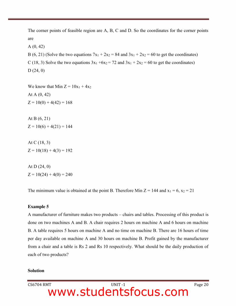
The corner points of feasible region are A, B, C and D. So the coordinates for the corner points
are
A (0, 42)
B (6, 21) (Solve the two equations 7x1 + 2x2 = 84 and 3x1 + 2x2 = 60 to get the coordinates)
C (18, 3) Solve the two equations 3x1 +6x2 = 72 and 3x1 + 2x2 = 60 to get the coordinates)
D (24, 0)
We know that Min Z = 10x1 + 4x2
At A (0, 42)
Z = 10(0) + 4(42) = 168
At B (6, 21)
Z = 10(6) + 4(21) = 144
At C (18, 3)
Z = 10(18) + 4(3) = 192
At D (24, 0)
Z = 10(24) + 4(0) = 240
The minimum value is obtained at the point B. Therefore Min Z = 144 and x1 = 6, x2 = 21
Example 5 A manufacturer of furniture makes two products – chairs and tables. Processing of this product is
done on two machines A and B. A chair requires 2 hours on machine A and 6 hours on machine
B. A table requires 5 hours on machine A and no time on machine B. There are 16 hours of time
per day available on machine A and 30 hours on machine B. Profit gained by the manufacturer
from a chair and a table is Rs 2 and Rs 10 respectively. What should be the daily production of
each of two products?
Solution
www.studentsfocus.com

SRI VIDYA COLLEGE OF ENGINEERING AND TECHNOLOGY COURSE MATERIAL (LECTURE NOTES)
CS6704 RMT UNIT -1 Page 21
Let x1 denotes the number of chairs
Let x2 denotes the number of tables
Chairs Tables Availability
Machine A
Machine B
2
6
5
0
16
30
Profit Rs 2 Rs 10
LPP Max Z = 2x1 + 10x2
Subject to
2x1+ 5x2 ≤ 16
6x1 + 0x2 ≤ 30
x1 ≥ 0 , x2 ≥ 0
Solving graphically The first constraint 2x1+ 5x2 ≤ 16, written in a form of equation
2x1+ 5x2 = 16
Put x1 = 0, then x2 = 16/5 = 3.2
Put x2 = 0, then x1 = 8
The coordinates are (0, 3.2) and (8, 0)
The second constraint 6x1 + 0x2 ≤ 30, written in a form of equation
6x1 = 30 → x1 =5
www.studentsfocus.com
SRI VIDYA COLLEGE OF ENGINEERING AND TECHNOLOGY COURSE MATERIAL (LECTURE NOTES)
CS6704 RMT UNIT -1 Page 22
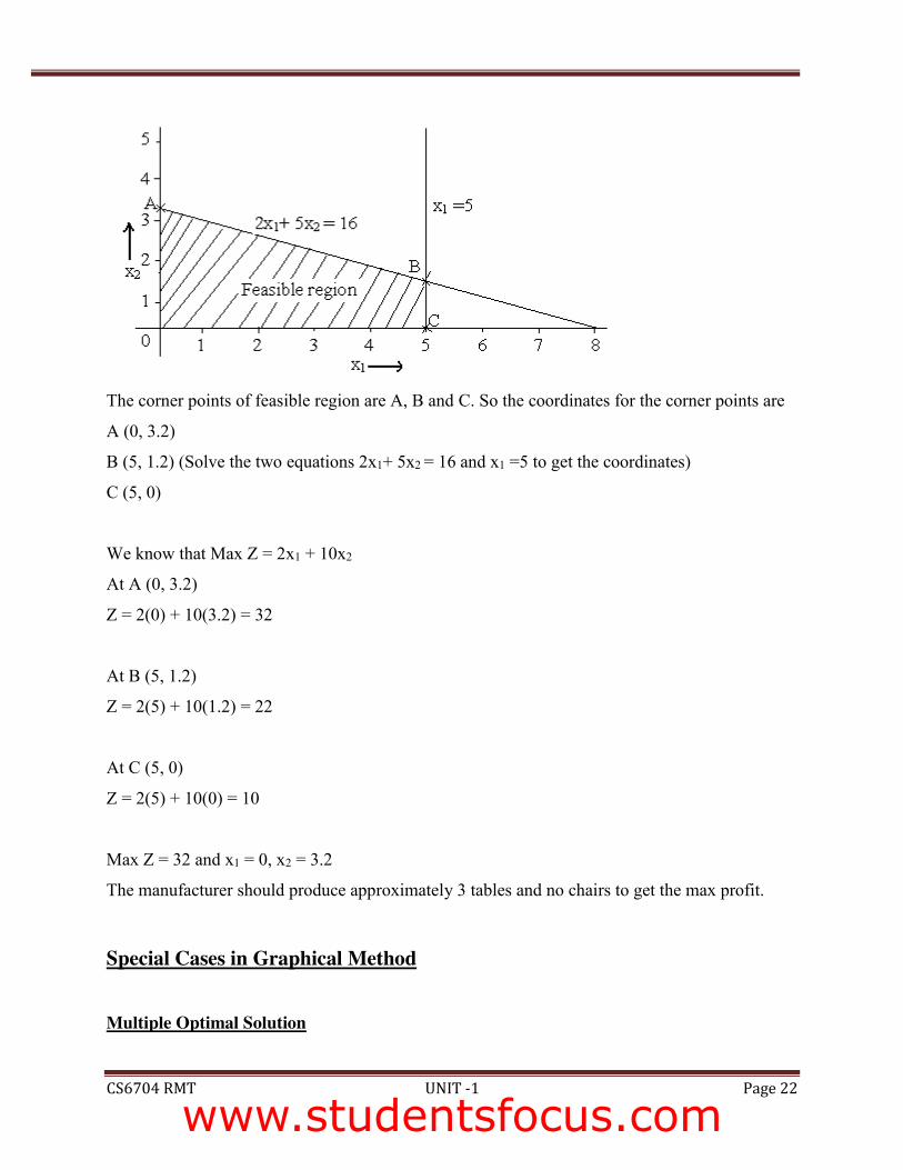
The corner points of feasible region are A, B and C. So the coordinates for the corner points are
A (0, 3.2)
B (5, 1.2) (Solve the two equations 2x1+ 5x2 = 16 and x1 =5 to get the coordinates)
C (5, 0)
We know that Max Z = 2x1 + 10x2
At A (0, 3.2)
Z = 2(0) + 10(3.2) = 32
At B (5, 1.2)
Z = 2(5) + 10(1.2) = 22
At C (5, 0)
Z = 2(5) + 10(0) = 10
Max Z = 32 and x1 = 0, x2 = 3.2
The manufacturer should produce approximately 3 tables and no chairs to get the max profit.
Special Cases in Graphical Method Multiple Optimal Solution
www.studentsfocus.com
SRI VIDYA COLLEGE OF ENGINEERING AND TECHNOLOGY COURSE MATERIAL (LECTURE NOTES)
CS6704 RMT UNIT -1 Page 23
Example 1 Solve by using graphical method
Max Z = 4x1 + 3x2
Subject to
4x1+ 3x2 ≤ 24
x1 ≤ 4.5
x2 ≤ 6
x1 ≥ 0 , x2 ≥ 0
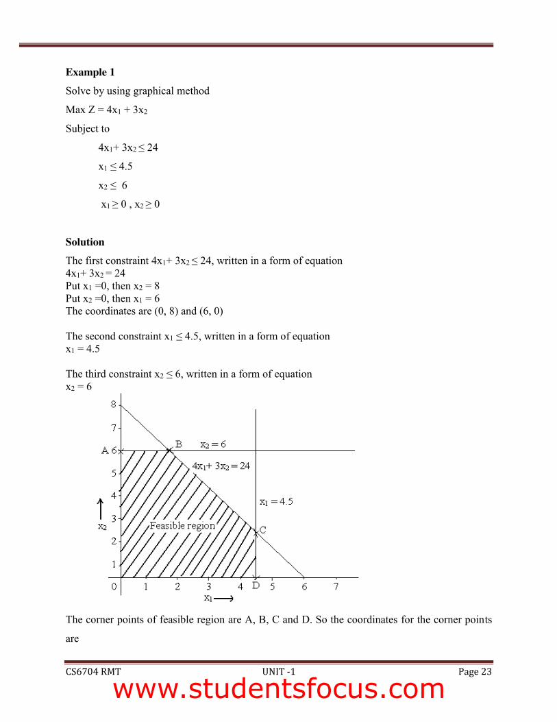
Solution The first constraint 4x1+ 3x2 ≤ 24, written in a form of equation 4x1+ 3x2 = 24 Put x1 =0, then x2 = 8 Put x2 =0, then x1 = 6 The coordinates are (0, 8) and (6, 0) The second constraint x1 ≤ 4.5, written in a form of equation x1 = 4.5 The third constraint x2 ≤ 6, written in a form of equation x2 = 6
The corner points of feasible region are A, B, C and D. So the coordinates for the corner points
are
www.studentsfocus.com

SRI VIDYA COLLEGE OF ENGINEERING AND TECHNOLOGY COURSE MATERIAL (LECTURE NOTES)
CS6704 RMT UNIT -1 Page 24
A (0, 6)
B (1.5, 6) (Solve the two equations 4x1+ 3x2 = 24 and x2 = 6 to get the coordinates)
C (4.5, 2) (Solve the two equations 4x1+ 3x2 = 24 and x1 = 4.5 to get the coordinates)
D (4.5, 0) We know that Max Z = 4x1 + 3x2 At A (0, 6) Z = 4(0) + 3(6) = 18 At B (1.5, 6) Z = 4(1.5) + 3(6) = 24 At C (4.5, 2) Z = 4(4.5) + 3(2) = 24 At D (4.5, 0) Z = 4(4.5) + 3(0) = 18 Max Z = 24, which is achieved at both B and C corner points. It can be achieved not only at B and C but every point between B and C. Hence the given problem has multiple optimal solutions.
3.4.2 No Optimal Solution Example 1 Solve graphically Max Z = 3x1 + 2x2 Subject to
x1+ x2 ≤ 1 x1+ x2 ≥ 3 x1 ≥ 0 , x2 ≥ 0
Solution The first constraint x1+ x2 ≤ 1, written in a form of equation x1+ x2 = 1 Put x1 =0, then x2 = 1 Put x2 =0, then x1 = 1 The coordinates are (0, 1) and (1, 0) The first constraint x1+ x2 ≥ 3, written in a form of equation
www.studentsfocus.com
SRI VIDYA COLLEGE OF ENGINEERING AND TECHNOLOGY COURSE MATERIAL (LECTURE NOTES)
CS6704 RMT UNIT -1 Page 25
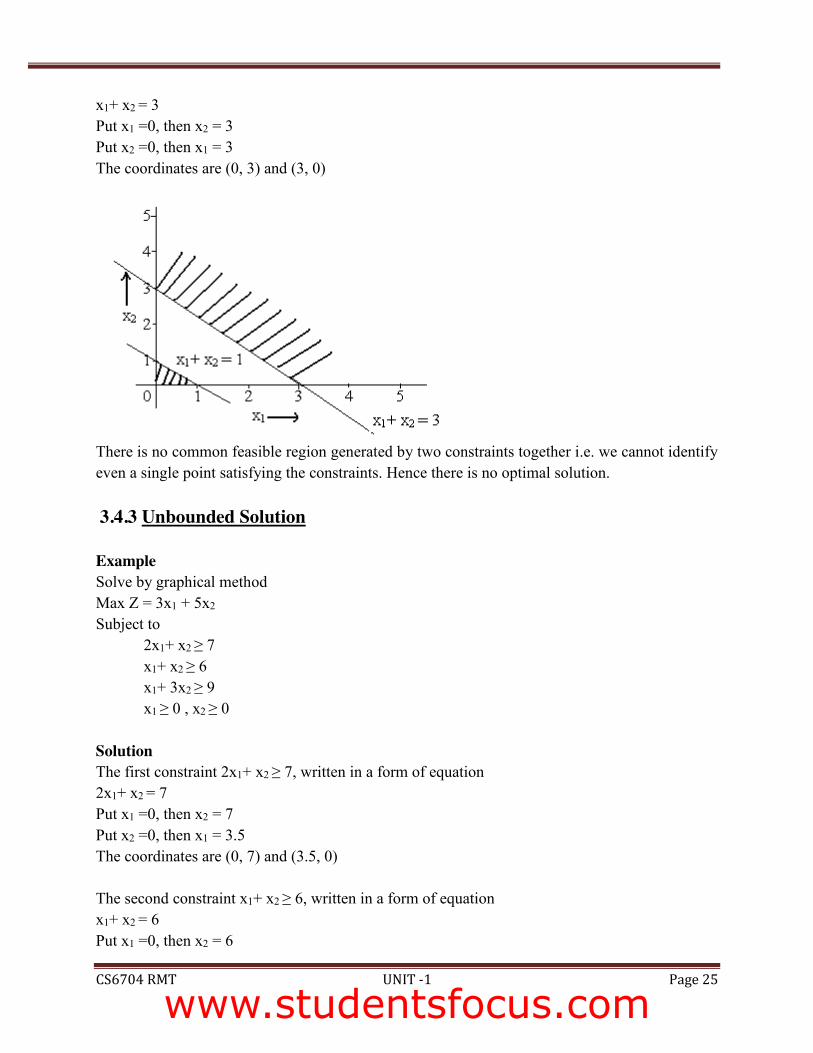
x1+ x2 = 3 Put x1 =0, then x2 = 3 Put x2 =0, then x1 = 3 The coordinates are (0, 3) and (3, 0)
There is no common feasible region generated by two constraints together i.e. we cannot identify even a single point satisfying the constraints. Hence there is no optimal solution.
3.4.3 Unbounded Solution Example Solve by graphical method Max Z = 3x1 + 5x2 Subject to
2x1+ x2 ≥ 7 x1+ x2 ≥ 6 x1+ 3x2 ≥ 9 x1 ≥ 0 , x2 ≥ 0
Solution The first constraint 2x1+ x2 ≥ 7, written in a form of equation 2x1+ x2 = 7 Put x1 =0, then x2 = 7 Put x2 =0, then x1 = 3.5 The coordinates are (0, 7) and (3.5, 0) The second constraint x1+ x2 ≥ 6, written in a form of equation x1+ x2 = 6 Put x1 =0, then x2 = 6
www.studentsfocus.com
SRI VIDYA COLLEGE OF ENGINEERING AND TECHNOLOGY COURSE MATERIAL (LECTURE NOTES)
CS6704 RMT UNIT -1 Page 26
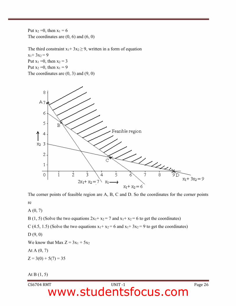
Put x2 =0, then x1 = 6 The coordinates are (0, 6) and (6, 0) The third constraint x1+ 3x2 ≥ 9, written in a form of equation x1+ 3x2 = 9 Put x1 =0, then x2 = 3 Put x2 =0, then x1 = 9 The coordinates are (0, 3) and (9, 0)
The corner points of feasible region are A, B, C and D. So the coordinates for the corner points
re
A (0, 7)
B (1, 5) (Solve the two equations 2x1+ x2 = 7 and x1+ x2 = 6 to get the coordinates)
C (4.5, 1.5) (Solve the two equations x1+ x2 = 6 and x1+ 3x2 = 9 to get the coordinates)
D (9, 0)
We know that Max Z = 3x1 + 5x2
At A (0, 7)
Z = 3(0) + 5(7) = 35
At B (1, 5)
www.studentsfocus.com
SRI VIDYA COLLEGE OF ENGINEERING AND TECHNOLOGY COURSE MATERIAL (LECTURE NOTES)
CS6704 RMT UNIT -1 Page 27
Z = 3(1) + 5(5) = 28 At C (4.5, 1.5) Z = 3(4.5) + 5(1.5) = 21 At D (9, 0) Z = 3(9) + 5(0) = 27 The values of objective function at corner points are 35, 28, 21 and 27. But there exists infinite number of points in the feasible region which is unbounded. The value of objective function will be more than the value of these four corner points i.e. the maximum value of the objective function occurs at a point at ∞. Hence the given problem has unbounded solution. Introduction
General Linear Programming Problem (GLPP) Maximize / Minimize Z = c1x1 + c2x2 + c3x3 +……………..+ cnxn
Subject to constraints
a11x1 + a12x2 + …..........+a1nxn (≤ or ≥) b1
a21x1 + a22x2 + ………..+a2nxn (≤ or ≥) b2
.
.
.
am1x1 + am2x2 + ……….+amnxn (≤ or ≥) bm
and
x1 ≥ 0, x2 ≥ 0,…, xn ≥ 0
Where constraints may be in the form of any inequality (≤ or ≥) or even in the form of an
equation (=) and finally satisfy the non-negativity restrictions.
Introduction to Simplex Method It was developed by G. Danztig in 1947. The simplex method provides an algorithm (a rule of
procedure usually involving repetitive application of a prescribed operation) which is based on
the fundamental theorem of linear programming.
The Simplex algorithm is an iterative procedure for solving LP problems in a finite number of
steps. It consists of
x Having a trial basic feasible solution to constraint-equations
www.studentsfocus.com
SRI VIDYA COLLEGE OF ENGINEERING AND TECHNOLOGY COURSE MATERIAL (LECTURE NOTES)
CS6704 RMT UNIT -1 Page 28
x Testing whether it is an optimal solution
x Improving the first trial solution by a set of rules and repeating the process till an optimal
solution is obtained
Advantages
x Simple to solve the problems
x The solution of LPP of more than two variables can be obtained. Computational Procedure of Simplex Method Consider an example Maximize Z = 3x1 + 2x2
Subject to
x1 + x2 ≤ 4
x1 – x2 ≤ 2
and x1 ≥ 0, x2 ≥ 0
Solution Step 1 – Write the given GLPP in the form of SLPP
Maximize Z = 3x1 + 2x2 + 0s1 + 0s2
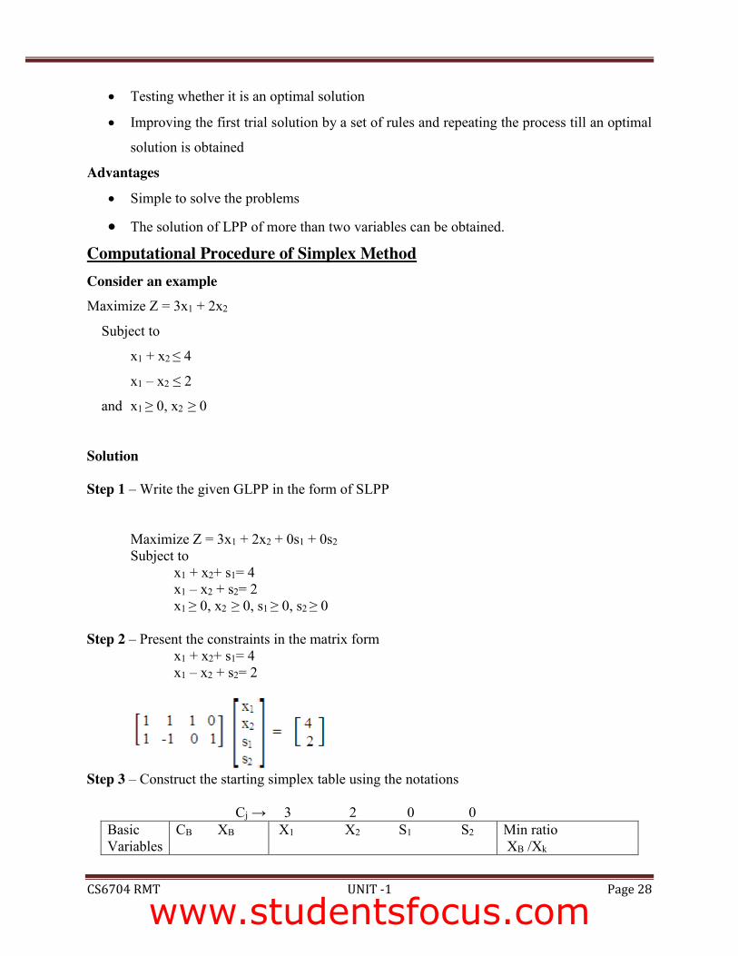
Subject to x1 + x2+ s1= 4 x1 – x2 + s2= 2 x1 ≥ 0, x2 ≥ 0, s1 ≥ 0, s2 ≥ 0 Step 2 – Present the constraints in the matrix form
x1 + x2+ s1= 4 x1 – x2 + s2= 2
Step 3 – Construct the starting simplex table using the notations Cj → 3 2 0 0
Basic Variables
CB XB X1 X2 S1 S2 Min ratio XB /Xk
www.studentsfocus.com
SRI VIDYA COLLEGE OF ENGINEERING AND TECHNOLOGY COURSE MATERIAL (LECTURE NOTES)
CS6704 RMT UNIT -1 Page 29
s1
s2
0 4 0 2
1 1 1 0 1 -1 0 1
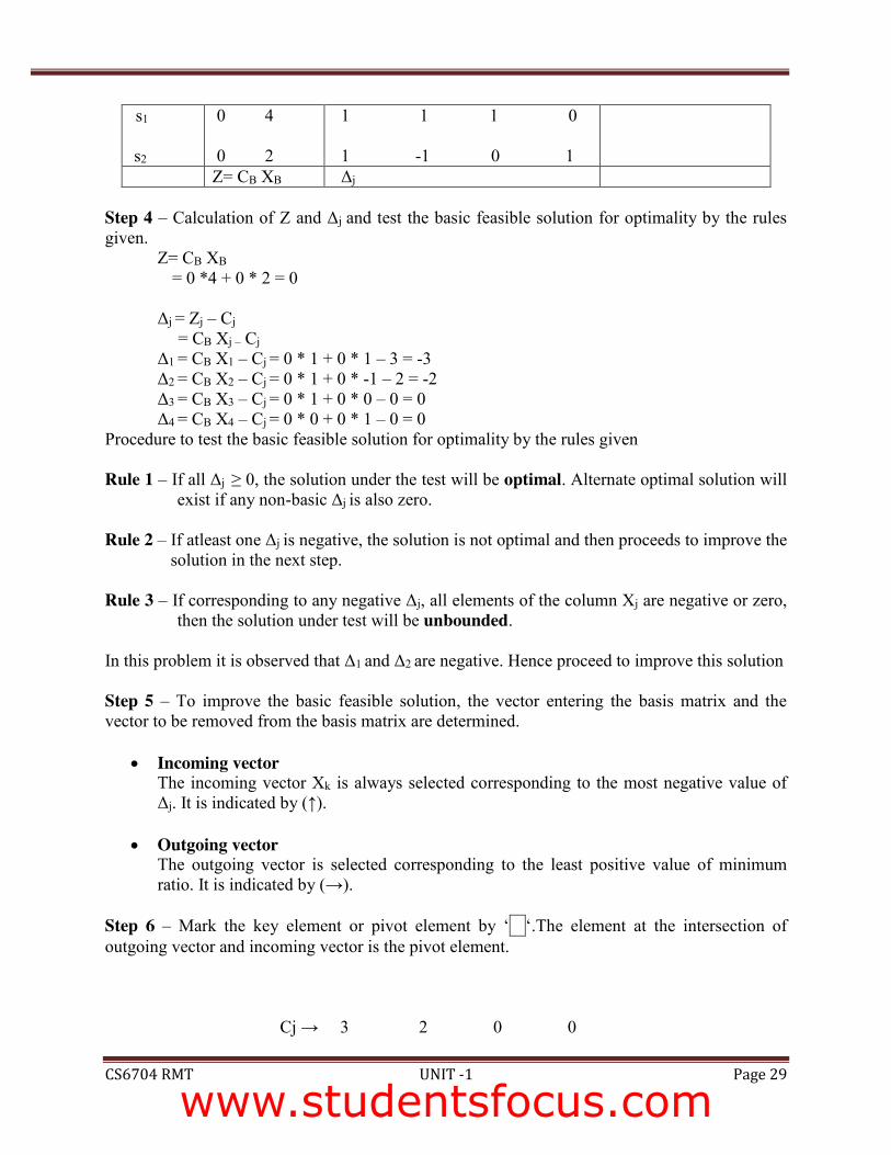
Z= CB XB Δj Step 4 – Calculation of Z and Δj and test the basic feasible solution for optimality by the rules given.
Z= CB XB
= 0 *4 + 0 * 2 = 0 Δj = Zj – Cj
= CB Xj – Cj Δ1 = CB X1 – Cj = 0 * 1 + 0 * 1 – 3 = -3 Δ2 = CB X2 – Cj = 0 * 1 + 0 * -1 – 2 = -2 Δ3 = CB X3 – Cj = 0 * 1 + 0 * 0 – 0 = 0 Δ4 = CB X4 – Cj = 0 * 0 + 0 * 1 – 0 = 0
Procedure to test the basic feasible solution for optimality by the rules given Rule 1 – If all Δj ≥ 0, the solution under the test will be optimal. Alternate optimal solution will
exist if any non-basic Δj is also zero. Rule 2 – If atleast one Δj is negative, the solution is not optimal and then proceeds to improve the
solution in the next step. Rule 3 – If corresponding to any negative Δj, all elements of the column Xj are negative or zero,
then the solution under test will be unbounded. In this problem it is observed that Δ1 and Δ2 are negative. Hence proceed to improve this solution Step 5 – To improve the basic feasible solution, the vector entering the basis matrix and the vector to be removed from the basis matrix are determined.
x Incoming vector The incoming vector Xk is always selected corresponding to the most negative value of Δj. It is indicated by (↑).
x Outgoing vector
The outgoing vector is selected corresponding to the least positive value of minimum ratio. It is indicated by (→).
Step 6 – Mark the key element or pivot element by ‘1’‘.The element at the intersection of outgoing vector and incoming vector is the pivot element.
Cj → 3 2 0 0
www.studentsfocus.com
SRI VIDYA COLLEGE OF ENGINEERING AND TECHNOLOGY COURSE MATERIAL (LECTURE NOTES)
CS6704 RMT UNIT -1 Page 30
Basic Variables
CB XB X1 X2 S1 S2 (Xk)
Min ratio XB /Xk
s1
s2
0 4 0 2
1 1 1 0 1 -1 0 1
4 / 1 = 4 2 / 1 = 2 → outgoing
Z= CB XB = 0
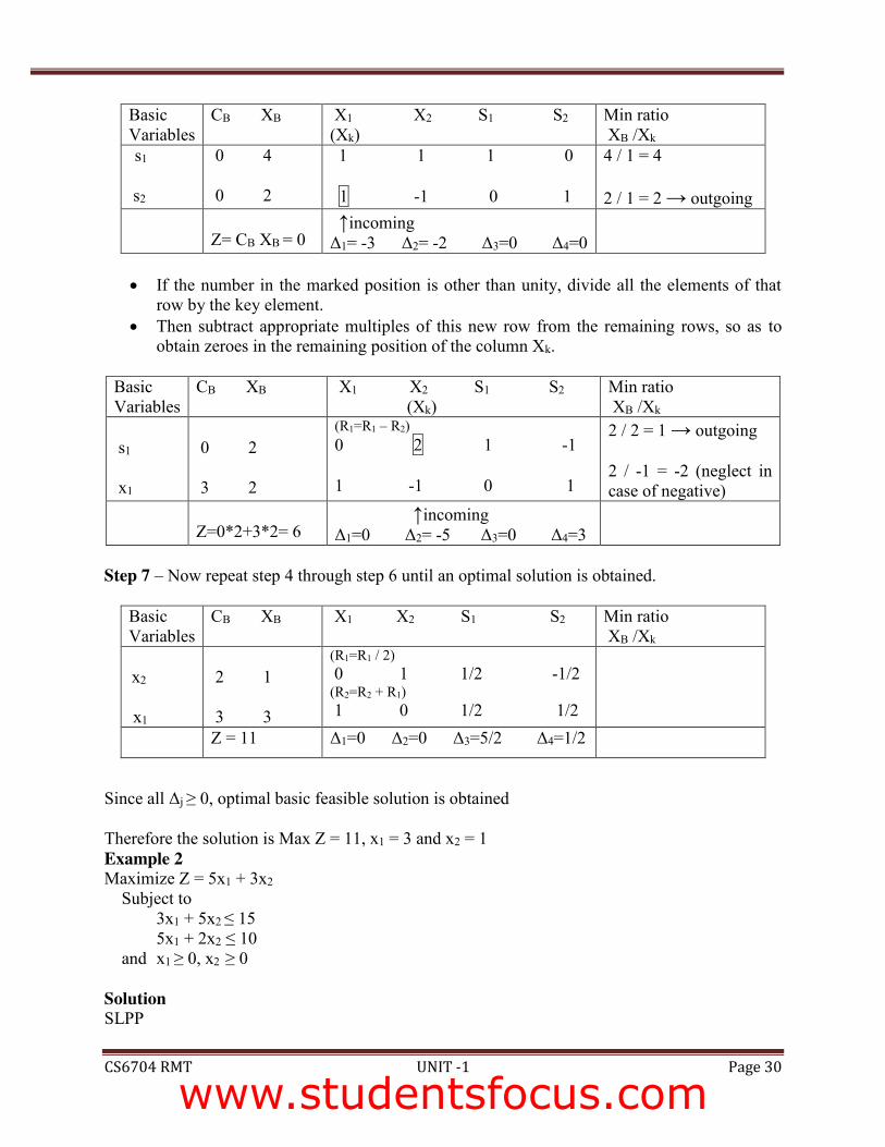
↑incoming Δ1= -3 Δ2= -2 Δ3=0 Δ4=0
x If the number in the marked position is other than unity, divide all the elements of that
row by the key element. x Then subtract appropriate multiples of this new row from the remaining rows, so as to
obtain zeroes in the remaining position of the column Xk.
Basic Variables
CB XB X1 X2 S1 S2 (Xk)
Min ratio XB /Xk
s1
x1
0 2 3 2
(R1=R1 – R2) 0 2 1 -1 1 -1 0 1
2 / 2 = 1 → outgoing 2 / -1 = -2 (neglect in case of negative)
Z=0*2+3*2= 6
↑incoming Δ1=0 Δ2= -5 Δ3=0 Δ4=3
Step 7 – Now repeat step 4 through step 6 until an optimal solution is obtained.
Basic Variables
CB XB X1 X2 S1 S2
Min ratio XB /Xk
x2
x1
2 1 3 3
(R1=R1 / 2) 0 1 1/2 -1/2 (R2=R2 + R1) 1 0 1/2 1/2
Z = 11 Δ1=0 Δ2=0 Δ3=5/2 Δ4=1/2
Since all Δj ≥ 0, optimal basic feasible solution is obtained Therefore the solution is Max Z = 11, x1 = 3 and x2 = 1 Example 2 Maximize Z = 5x1 + 3x2 Subject to 3x1 + 5x2 ≤ 15 5x1 + 2x2 ≤ 10 and x1 ≥ 0, x2 ≥ 0 Solution SLPP
www.studentsfocus.com
SRI VIDYA COLLEGE OF ENGINEERING AND TECHNOLOGY COURSE MATERIAL (LECTURE NOTES)
CS6704 RMT UNIT -1 Page 31
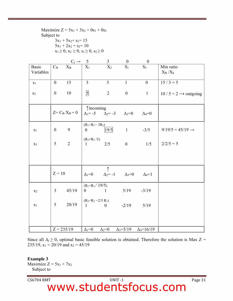
Maximize Z = 5x1 + 3x2 + 0s1 + 0s2 Subject to 3x1 + 5x2+ s1= 15 5x1 + 2x2 + s2= 10 x1 ≥ 0, x2 ≥ 0, s1 ≥ 0, s2 ≥ 0
Cj → 5 3 0 0
Basic Variables
CB XB X1 X2 S1 S2
Min ratio XB /Xk
s1
s2
0 15 0 10
3 5 1 0 5 2 0 1
15 / 3 = 5 10 / 5 = 2 → outgoing
Z= CB XB = 0
↑incoming Δ1= -5 Δ2= -3 Δ3=0 Δ4=0
s1 x1
0 9 5 2
(R1=R1– 3R2) 0 19/5 1 -3/5 (R2=R2 /5) 1 2/5 0 1/5
9/19/5 = 45/19 → 2/2/5 = 5
Z = 10
↑ Δ1=0 Δ2= -1 Δ3=0 Δ4=1
x2 x1
3 45/19 5 20/19
(R1=R1 / 19/5) 0 1 5/19 -3/19 (R2=R2 –2/5 R1) 1 0 -2/19 5/19
Z = 235/19 Δ1=0 Δ2=0 Δ3=5/19 Δ4=16/19 Since all Δj ≥ 0, optimal basic feasible solution is obtained. Therefore the solution is Max Z = 235/19, x1 = 20/19 and x2 = 45/19 Example 3 Maximize Z = 5x1 + 7x2 Subject to
www.studentsfocus.com
SRI VIDYA COLLEGE OF ENGINEERING AND TECHNOLOGY COURSE MATERIAL (LECTURE NOTES)
CS6704 RMT UNIT -1 Page 32
x1 + x2 ≤ 4 3x1 – 8x2 ≤ 24 10x1 + 7x2 ≤ 35 and x1 ≥ 0, x2 ≥ 0 Solution SLPP
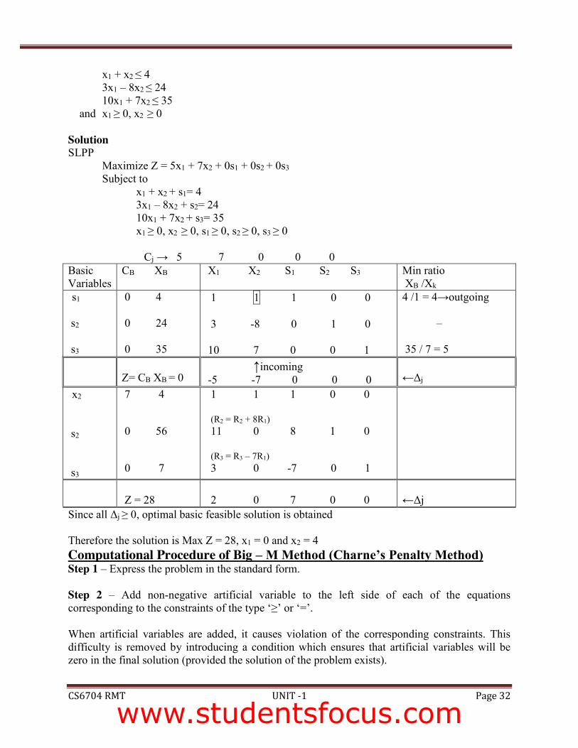
Maximize Z = 5x1 + 7x2 + 0s1 + 0s2 + 0s3 Subject to x1 + x2 + s1= 4 3x1 – 8x2 + s2= 24 10x1 + 7x2 + s3= 35 x1 ≥ 0, x2 ≥ 0, s1 ≥ 0, s2 ≥ 0, s3 ≥ 0 Cj → 5 7 0 0 0 Basic Variables
CB XB X1 X2 S1 S2 S3
Min ratio XB /Xk
s1
s2
s3
0 4 0 24
0 35
1 1 1 0 0 3 -8 0 1 0 10 7 0 0 1
4 /1 = 4→outgoing
–
35 / 7 = 5
Z= CB XB = 0 ↑incoming -5 -7 0 0 0
←Δj
x2
s2 s3
7 4 0 56
0 7
1 1 1 0 0 (R2 = R2 + 8R1) 11 0 8 1 0 (R3 = R3 – 7R1) 3 0 -7 0 1
Z = 28
2 0 7 0 0
←Δj
Since all Δj ≥ 0, optimal basic feasible solution is obtained Therefore the solution is Max Z = 28, x1 = 0 and x2 = 4 Computational Procedure of Big – M Method (Charne’s Penalty Method) Step 1 – Express the problem in the standard form. Step 2 – Add non-negative artificial variable to the left side of each of the equations corresponding to the constraints of the type ‘≥’ or ‘=’. When artificial variables are added, it causes violation of the corresponding constraints. This difficulty is removed by introducing a condition which ensures that artificial variables will be zero in the final solution (provided the solution of the problem exists).
www.studentsfocus.com
SRI VIDYA COLLEGE OF ENGINEERING AND TECHNOLOGY COURSE MATERIAL (LECTURE NOTES)
CS6704 RMT UNIT -1 Page 33
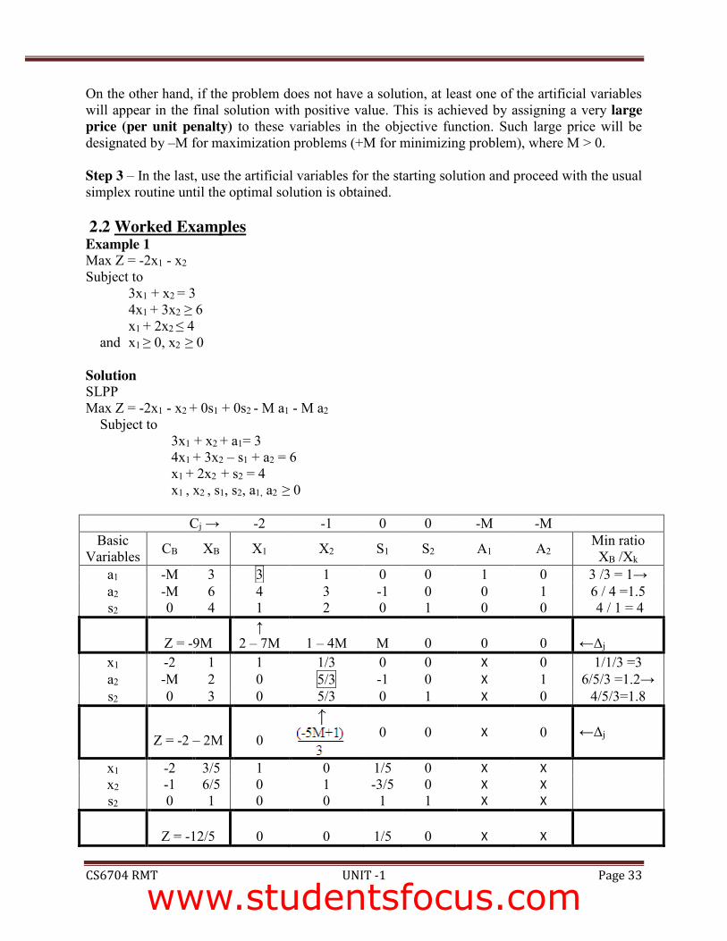
On the other hand, if the problem does not have a solution, at least one of the artificial variables will appear in the final solution with positive value. This is achieved by assigning a very large price (per unit penalty) to these variables in the objective function. Such large price will be designated by –M for maximization problems (+M for minimizing problem), where M > 0. Step 3 – In the last, use the artificial variables for the starting solution and proceed with the usual simplex routine until the optimal solution is obtained. 2.2 Worked Examples Example 1 Max Z = -2x1 - x2 Subject to 3x1 + x2 = 3 4x1 + 3x2 ≥ 6 x1 + 2x2 ≤ 4 and x1 ≥ 0, x2 ≥ 0 Solution SLPP Max Z = -2x1 - x2 + 0s1 + 0s2 - M a1 - M a2 Subject to 3x1 + x2 + a1= 3 4x1 + 3x2 – s1 + a2 = 6 x1 + 2x2 + s2 = 4 x1 , x2 , s1, s2, a1, a2 ≥ 0
Cj → -2 -1 0 0 -M -M
Basic Variables CB XB X1 X2 S1 S2 A1 A2
Min ratio XB /Xk
a1 -M 3 3 1 0 0 1 0 3 /3 = 1→ a2 -M 6 4 3 -1 0 0 1 6 / 4 =1.5 s2 0 4 1 2 0 1 0 0 4 / 1 = 4
Z = -9M
↑ 2 – 7M
1 – 4M
M
0
0
0
←Δj
x1 -2 1 1 1/3 0 0 X 0 1/1/3 =3 a2 -M 2 0 5/3 -1 0 X 1 6/5/3 =1.2→ s2 0 3 0 5/3 0 1 X 0 4/5/3=1.8
Z = -2 – 2M
0
0 0 X 0
←Δj
x1 -2 3/5 1 0 1/5 0 X X x2 -1 6/5 0 1 -3/5 0 X X s2 0 1 0 0 1 1 X X
Z = -12/5
0
0
1/5
0
X
X
www.studentsfocus.com
SRI VIDYA COLLEGE OF ENGINEERING AND TECHNOLOGY COURSE MATERIAL (LECTURE NOTES)
CS6704 RMT UNIT -1 Page 34
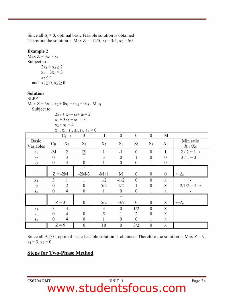
Since all Δj ≥ 0, optimal basic feasible solution is obtained Therefore the solution is Max Z = -12/5, x1 = 3/5, x2 = 6/5 Example 2 Max Z = 3x1 - x2 Subject to 2x1 + x2 ≥ 2 x1 + 3x2 ≤ 3 x2 ≤ 4 and x1 ≥ 0, x2 ≥ 0 Solution SLPP Max Z = 3x1 - x2 + 0s1 + 0s2 + 0s3 - M a1 Subject to 2x1 + x2 – s1+ a1= 2 x1 + 3x2 + s2 = 3 x2 + s3 = 4 x1 , x2 , s1, s2, s3, a1 ≥ 0
Cj → 3 -1 0 0 0 -M Basic
Variables CB XB X1 X2 S1 S2 S3 A1 Min ratio XB /Xk
a1 -M 2 2 1 -1 0 0 1 2 / 2 = 1→ s2 0 3 1 3 0 1 0 0 3 / 1 = 3 s3 0 4 0 1 0 0 1 0 -
Z = -2M
↑ -2M-3
-M+1
M
0
0
0
←Δj
x1 3 1 1 1/2 -1/2 0 0 X - s2 0 2 0 5/2 1/2 1 0 X 2/1/2 = 4→ s3 0 4 0 1 0 0 1 X -
Z = 3
0
5/2
↑ -3/2
0
0
X
←Δj
x1 3 3 1 3 0 1/2 0 X s1 0 4 0 5 1 2 0 X s3 0 4 0 1 0 0 1 X Z = 9 0 10 0 3/2 0 X
Since all Δj ≥ 0, optimal basic feasible solution is obtained. Therefore the solution is Max Z = 9, x1 = 3, x2 = 0 Steps for Two-Phase Method
www.studentsfocus.com
SRI VIDYA COLLEGE OF ENGINEERING AND TECHNOLOGY COURSE MATERIAL (LECTURE NOTES)
CS6704 RMT UNIT -1 Page 35
The process of eliminating artificial variables is performed in phase-I of the solution and phase-II is used to get an optimal solution. Since the solution of LPP is computed in two phases, it is called as Two-Phase Simplex Method. Phase I – In this phase, the simplex method is applied to a specially constructed auxiliary linear programming problem leading to a final simplex table containing a basic feasible solution to the original problem.
Step 1 – Assign a cost -1 to each artificial variable and a cost 0 to all other variables in the objective function. Step 2 – Construct the Auxiliary LPP in which the new objective function Z* is to be maximized subject to the given set of constraints. Step 3 – Solve the auxiliary problem by simplex method until either of the following three possibilities do arise
i. Max Z* < 0 and atleast one artificial vector appear in the optimum basis at a positive level (Δj ≥ 0). In this case, given problem does not possess any feasible solution.
ii. Max Z* = 0 and at least one artificial vector appears in the optimum basis at a zero level. In this case proceed to phase-II.
iii. Max Z* = 0 and no one artificial vector appears in the optimum basis. In this case also proceed to phase-II.
Phase II – Now assign the actual cost to the variables in the objective function and a zero cost to every artificial variable that appears in the basis at the zero level. This new objective function is now maximized by simplex method subject to the given constraints. Simplex method is applied to the modified simplex table obtained at the end of phase-I, until an optimum basic feasible solution has been attained. The artificial variables which are non-basic at the end of phase-I are removed. Worked Examples Example 1 Max Z = 3x1 - x2 Subject to 2x1 + x2 ≥ 2 x1 + 3x2 ≤ 2 x2 ≤ 4 and x1 ≥ 0, x2 ≥ 0 Solution Standard LPP Max Z = 3x1 - x2 Subject to 2x1 + x2 – s1+ a1= 2
www.studentsfocus.com
SRI VIDYA COLLEGE OF ENGINEERING AND TECHNOLOGY COURSE MATERIAL (LECTURE NOTES)
CS6704 RMT UNIT -1 Page 36
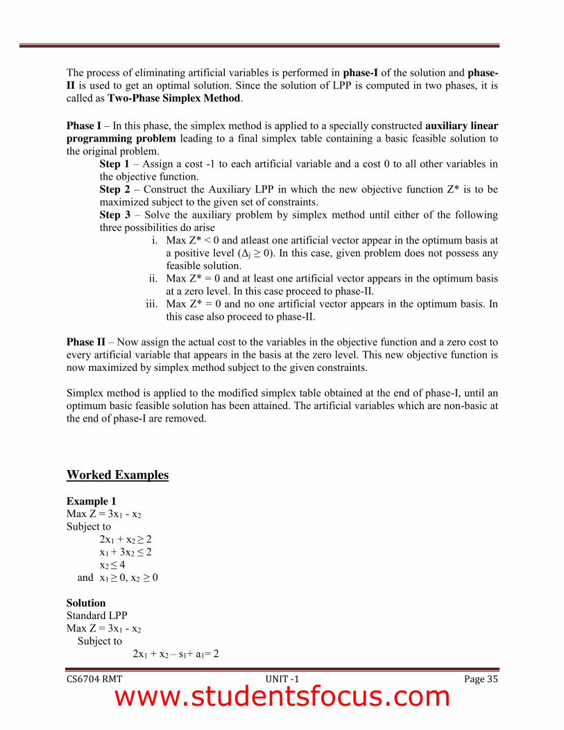
x1 + 3x2 + s2 = 2 x2 + s3 = 4 x1 , x2 , s1, s2, s3,a1 ≥ 0 Auxiliary LPP Max Z* = 0x1 - 0x2 + 0s1 + 0s2 + 0s3 -1a1 Subject to 2x1 + x2 – s1+ a1= 2 x1 + 3x2 + s2 = 2 x2 + s3 = 4 x1 , x2 , s1, s2, s3,a1 ≥ 0 Phase I
Cj → 0 0 0 0 0 -1 Basic
Variables CB XB X1 X2 S1 S2 S3 A1 Min ratio XB /Xk
a1 -1 2 2 1 -1 0 0 1 1→ s2 0 2 1 3 0 1 0 0 2 s3 0 4 0 1 0 0 1 0 -
Z* = -2
↑ -2
-1
1
0
0
0
←Δj
x1 0 1 1 1/2 -1/2 0 0 X s2 0 1 0 5/2 1/2 1 0 X s3 0 4 0 1 0 0 1 X
Z* = 0
0
0
0
0
0
X
←Δj
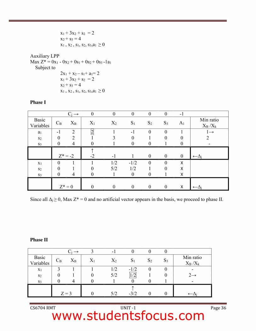
Since all Δj ≥ 0, Max Z* = 0 and no artificial vector appears in the basis, we proceed to phase II. Phase II
Cj → 3 -1 0 0 0 Basic
Variables CB XB X1 X2 S1 S2 S3 Min ratio XB /Xk
x1 3 1 1 1/2 -1/2 0 0 - s2 0 1 0 5/2 1/2 1 0 2→ s3 0 4 0 1 0 0 1 -
Z = 3
0
5/2
↑ -3/2
0
0
←Δj
www.studentsfocus.com
SRI VIDYA COLLEGE OF ENGINEERING AND TECHNOLOGY COURSE MATERIAL (LECTURE NOTES)
CS6704 RMT UNIT -1 Page 37
x1 3 2 1 3 0 1 0 s1 0 2 0 5 1 2 0 s3 0 4 0 1 0 0 1
Z = 6
0
10
0
3
0
←Δj
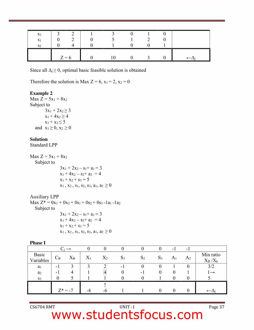
Since all Δj ≥ 0, optimal basic feasible solution is obtained Therefore the solution is Max Z = 6, x1 = 2, x2 = 0 Example 2 Max Z = 5x1 + 8x2 Subject to
3x1 + 2x2 ≥ 3 x1 + 4x2 ≥ 4 x1 + x2 ≤ 5
and x1 ≥ 0, x2 ≥ 0 Solution Standard LPP Max Z = 5x1 + 8x2 Subject to 3x1 + 2x2 – s1+ a1 = 3 x1 + 4x2 – s2+ a2 = 4 x1 + x2 + s3 = 5 x1 , x2 , s1, s2, s3, a1, a2 ≥ 0 Auxiliary LPP Max Z* = 0x1 + 0x2 + 0s1 + 0s2 + 0s3 -1a1 -1a2 Subject to 3x1 + 2x2 – s1+ a1 = 3 x1 + 4x2 – s2+ a2 = 4 x1 + x2 + s3 = 5 x1 , x2 , s1, s2, s3, a1, a2 ≥ 0 Phase I
Cj → 0 0 0 0 0 -1 -1 Basic
Variables CB XB X1 X2 S1 S2 S3 A1 A2 Min ratio XB /Xk
a1 -1 3 3 2 -1 0 0 1 0 3/2 a2 -1 4 1 4 0 -1 0 0 1 1→ s3 0 5 1 1 0 0 1 0 0 5
Z* = -7
-4
↑ -6
1
1
0
0
0
←Δj
www.studentsfocus.com
SRI VIDYA COLLEGE OF ENGINEERING AND TECHNOLOGY COURSE MATERIAL (LECTURE NOTES)
CS6704 RMT UNIT -1 Page 38
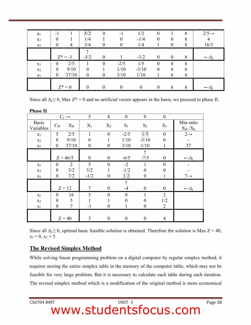
a1 -1 1 5/2 0 -1 1/2 0 1 X 2/5→ x2 0 1 1/4 1 0 -1/4 0 0 X 4 s3 0 4 3/4 0 0 1/4 1 0 X 16/3
Z* = -1
↑ -5/2
0
1
-1/2
0
0
X
←Δj
x1 0 2/5 1 0 -2/5 1/5 0 X X x2 0 9/10 0 1 1/10 -3/10 0 X X s3 0 37/10 0 0 3/10 1/10 1 X X
Z* = 0
0
0
0
0
0
X
X
←Δj
Since all Δj ≥ 0, Max Z* = 0 and no artificial vector appears in the basis, we proceed to phase II. Phase II
Cj → 5 8 0 0 0 Basic
Variables CB XB X1 X2 S1 S2 S3 Min ratio XB /Xk
x1 5 2/5 1 0 -2/5 1/5 0 2→ x2 8 9/10 0 1 1/10 -3/10 0 - s3 0 37/10 0 0 3/10 1/10 1 37
Z = 46/5
0
0
-6/5
↑ -7/5
0
←Δj
s2 0 2 5 0 -2 1 0 - x2 8 3/2 3/2 1 -1/2 0 0 - s3 0 7/2 -1/2 0 1/2 0 1 7→
Z = 12
7
0
↑ -4
0
0
←Δj
s2 0 16 3 0 0 1 2 x2 8 5 1 1 0 0 1/2 s1 0 7 -1 0 1 0 2
Z = 40
3
0
0
0
4
Since all Δj ≥ 0, optimal basic feasible solution is obtained. Therefore the solution is Max Z = 40, x1 = 0, x2 = 5 The Revised Simplex Method While solving linear programming problem on a digital computer by regular simplex method, it
requires storing the entire simplex table in the memory of the computer table, which may not be
feasible for very large problem. But it is necessary to calculate each table during each iteration.
The revised simplex method which is a modification of the original method is more economical
www.studentsfocus.com
SRI VIDYA COLLEGE OF ENGINEERING AND TECHNOLOGY COURSE MATERIAL (LECTURE NOTES)
CS6704 RMT UNIT -1 Page 39
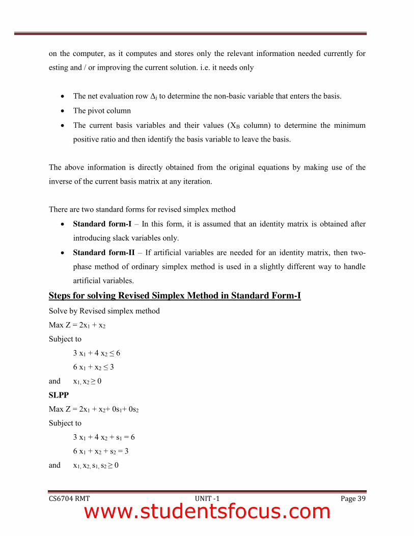
on the computer, as it computes and stores only the relevant information needed currently for
esting and / or improving the current solution. i.e. it needs only
x The net evaluation row Δj to determine the non-basic variable that enters the basis.
x The pivot column
x The current basis variables and their values (XB column) to determine the minimum
positive ratio and then identify the basis variable to leave the basis.
The above information is directly obtained from the original equations by making use of the
inverse of the current basis matrix at any iteration.
There are two standard forms for revised simplex method
x Standard form-I – In this form, it is assumed that an identity matrix is obtained after
introducing slack variables only.
x Standard form-II – If artificial variables are needed for an identity matrix, then two-
phase method of ordinary simplex method is used in a slightly different way to handle
artificial variables.
Steps for solving Revised Simplex Method in Standard Form-I
Solve by Revised simplex method
Max Z = 2x1 + x2
Subject to
3 x1 + 4 x2 ≤ 6
6 x1 + x2 ≤ 3
and x1, x2 ≥ 0
SLPP Max Z = 2x1 + x2+ 0s1+ 0s2
Subject to
3 x1 + 4 x2 + s1 = 6
6 x1 + x2 + s2 = 3
and x1, x2, s1, s2 ≥ 0
www.studentsfocus.com
SRI VIDYA COLLEGE OF ENGINEERING AND TECHNOLOGY COURSE MATERIAL (LECTURE NOTES)
CS6704 RMT UNIT -1 Page 40
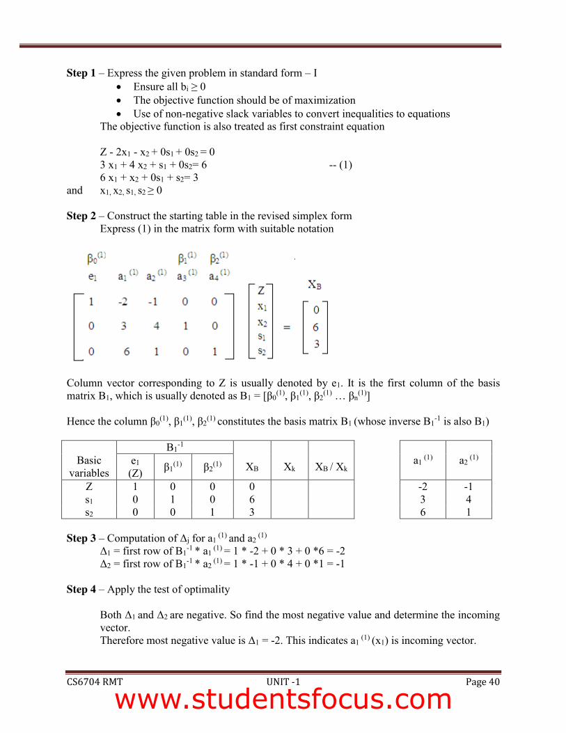
Step 1 – Express the given problem in standard form – I x Ensure all bi ≥ 0 x The objective function should be of maximization x Use of non-negative slack variables to convert inequalities to equations
The objective function is also treated as first constraint equation
Z - 2x1 - x2 + 0s1 + 0s2 = 0 3 x1 + 4 x2 + s1 + 0s2= 6 -- (1) 6 x1 + x2 + 0s1 + s2= 3 and x1, x2, s1, s2 ≥ 0 Step 2 – Construct the starting table in the revised simplex form
Express (1) in the matrix form with suitable notation
Column vector corresponding to Z is usually denoted by e1. It is the first column of the basis matrix B1, which is usually denoted as B1 = [β0
(1), β1(1), β2
(1) … βn(1)]
Hence the column β0
(1), β1(1), β2
(1) constitutes the basis matrix B1 (whose inverse B1-1 is also B1)
Basic variables
B1-1
XB
Xk
XB / Xk
a1
(1)
a2
(1)
e1 (Z) β1
(1) β2(1)
Z 1 0 0 0 -2 -1 s1 0 1 0 6 3 4 s2 0 0 1 3 6 1
Step 3 – Computation of Δj for a1
(1) and a2 (1)
Δ1 = first row of B1-1 * a1
(1) = 1 * -2 + 0 * 3 + 0 *6 = -2 Δ2 = first row of B1
-1 * a2 (1) = 1 * -1 + 0 * 4 + 0 *1 = -1
Step 4 – Apply the test of optimality
Both Δ1 and Δ2 are negative. So find the most negative value and determine the incoming vector. Therefore most negative value is Δ1 = -2. This indicates a1
(1) (x1) is incoming vector.
www.studentsfocus.com
SRI VIDYA COLLEGE OF ENGINEERING AND TECHNOLOGY COURSE MATERIAL (LECTURE NOTES)
CS6704 RMT UNIT -1 Page 41
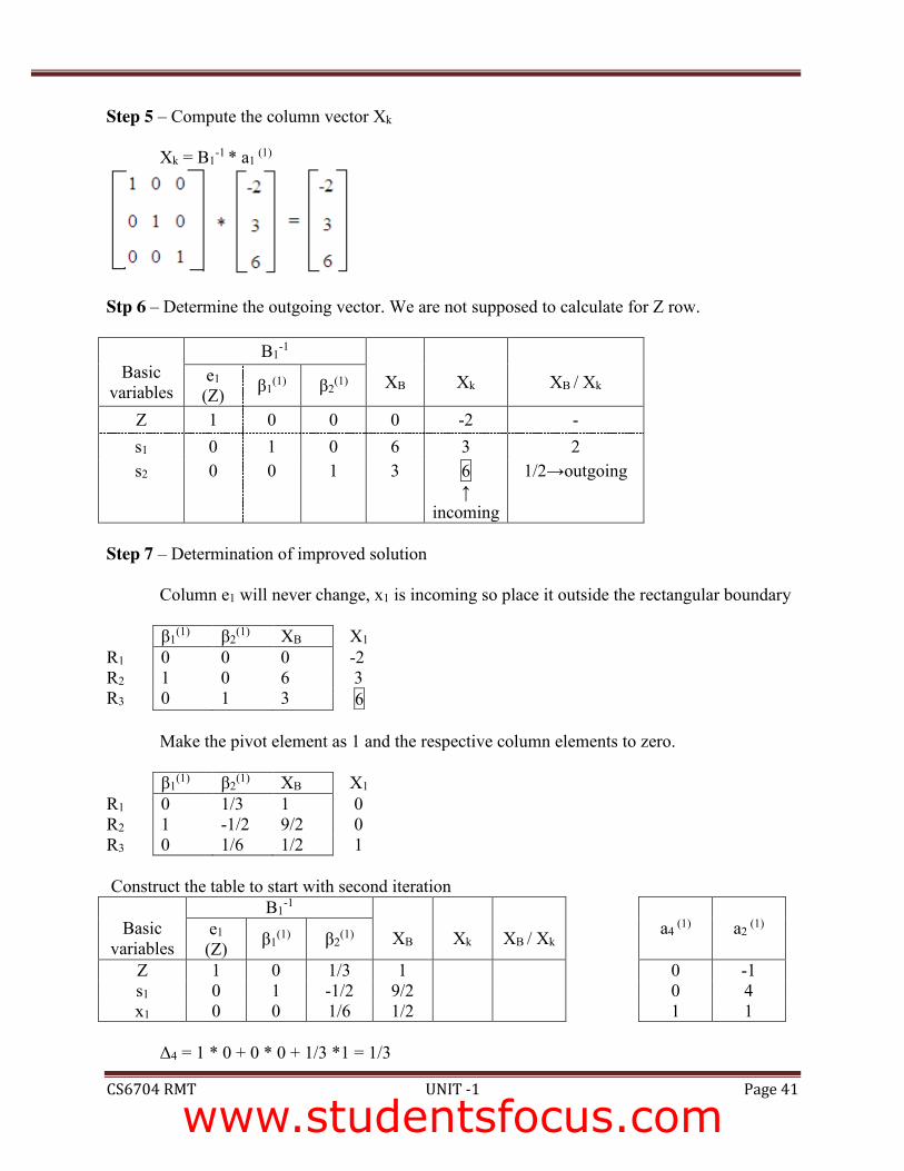
Step 5 – Compute the column vector Xk Xk = B1
-1 * a1 (1)
Stp 6 – Determine the outgoing vector. We are not supposed to calculate for Z row.
Basic
variables
B1-1
XB
Xk
XB / Xk e1 (Z) β1
(1) β2(1)
Z 1 0 0 0 -2 - s1 0 1 0 6 3 2 s2
0
0
1
3
6 ↑
incoming
1/2→outgoing
Step 7 – Determination of improved solution Column e1 will never change, x1 is incoming so place it outside the rectangular boundary
β1
(1) β2(1) XB X1
R1 0 0 0 -2 R2 1 0 6 3 R3 0 1 3 6
Make the pivot element as 1 and the respective column elements to zero.
β1(1) β2
(1) XB X1 R1 0 1/3 1 0 R2 1 -1/2 9/2 0 R3 0 1/6 1/2 1
Construct the table to start with second iteration
Basic
variables
B1-1
XB
Xk
XB / Xk
a4
(1)
a2
(1)
e1 (Z) β1
(1) β2(1)
Z 1 0 1/3 1 0 -1 s1 0 1 -1/2 9/2 0 4 x1 0 0 1/6 1/2 1 1
Δ4 = 1 * 0 + 0 * 0 + 1/3 *1 = 1/3
www.studentsfocus.com
SRI VIDYA COLLEGE OF ENGINEERING AND TECHNOLOGY COURSE MATERIAL (LECTURE NOTES)
CS6704 RMT UNIT -1 Page 42
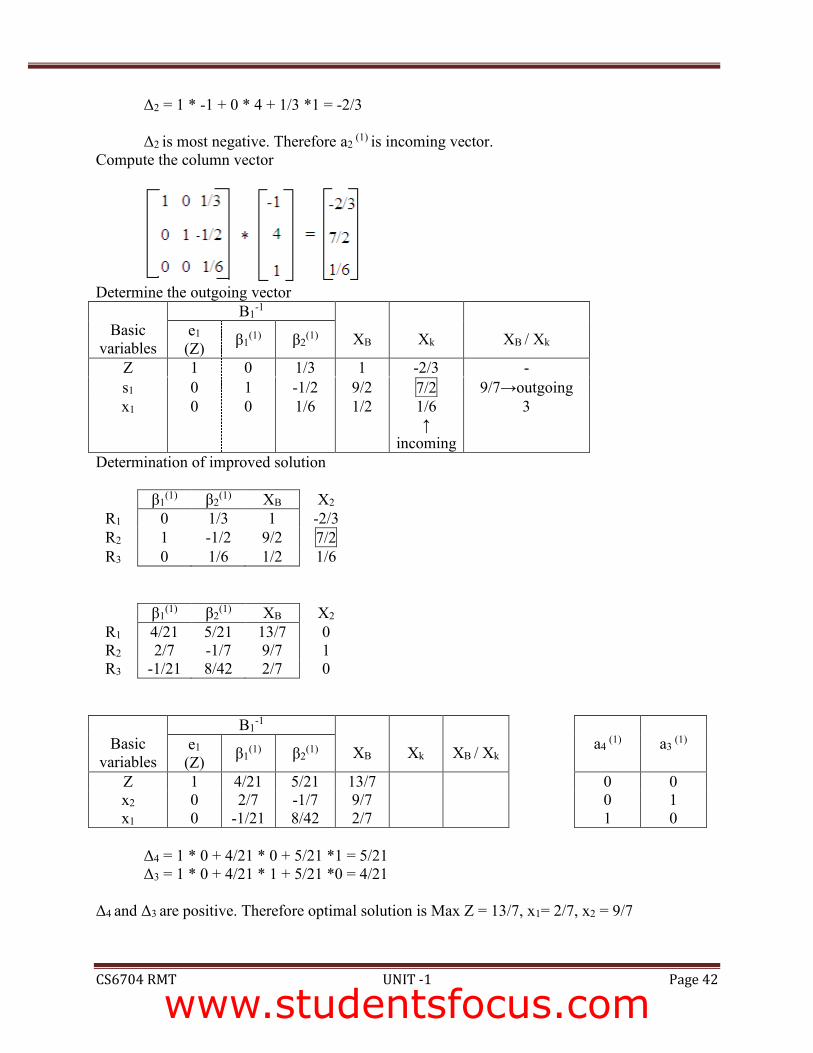
Δ2 = 1 * -1 + 0 * 4 + 1/3 *1 = -2/3
Δ2 is most negative. Therefore a2 (1) is incoming vector.
Compute the column vector
Determine the outgoing vector
Basic
variables
B1-1
XB
Xk
XB / Xk e1 (Z) β1
(1) β2(1)
Z 1 0 1/3 1 -2/3 - s1 0 1 -1/2 9/2 7/2 9/7→outgoing x1
0
0
1/6
1/2
1/6 ↑
incoming
3
Determination of improved solution
β1(1) β2
(1) XB X2 R1 0 1/3 1 -2/3 R2 1 -1/2 9/2 7/2 R3 0 1/6 1/2 1/6
β1(1) β2
(1) XB X2 R1 4/21 5/21 13/7 0 R2 2/7 -1/7 9/7 1 R3 -1/21 8/42 2/7 0
Basic
variables
B1-1
XB
Xk
XB / Xk
a4
(1)
a3
(1)
e1 (Z) β1
(1) β2(1)
Z 1 4/21 5/21 13/7 0 0 x2 0 2/7 -1/7 9/7 0 1 x1 0 -1/21 8/42 2/7 1 0
Δ4 = 1 * 0 + 4/21 * 0 + 5/21 *1 = 5/21
Δ3 = 1 * 0 + 4/21 * 1 + 5/21 *0 = 4/21 Δ4 and Δ3 are positive. Therefore optimal solution is Max Z = 13/7, x1= 2/7, x2 = 9/7
www.studentsfocus.com