1

Squircular Calculations

Chamberlain Fong

spectralfft@yahoo.com

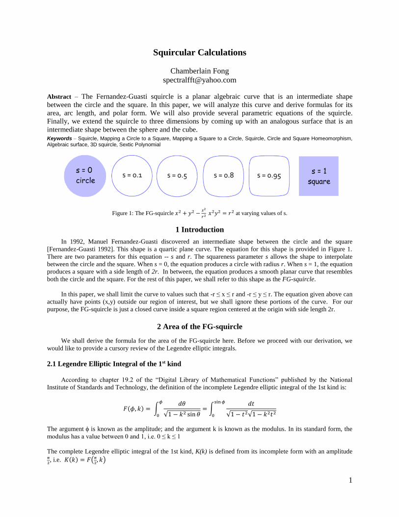
Abstract – The Fernandez-Guasti squircle is a planar algebraic curve that is an intermediate shape

between the circle and the square. In this paper, we will analyze this curve and derive formulas for its

area, arc length, and polar form. We will also provide several parametric equations of the squircle.

Finally, we extend the squircle to three dimensions by coming up with an analogous surface that is an

intermediate shape between the sphere and the cube.

Keywords – Squircle, Mapping a Circle to a Square, Mapping a Square to a Circle, Squircle, Circle and Square Homeomorphism, Algebraic surface, 3D squircle, Sextic Polynomial

Figure 1: The FG-squircle 𝑥2 + 𝑦2 −

𝑠2

𝑟2 𝑥2𝑦2 = 𝑟2 at varying values of s.

1 Introduction

In 1992, Manuel Fernandez-Guasti discovered an intermediate shape between the circle and the square

[Fernandez-Guasti 1992]. This shape is a quartic plane curve. The equation for this shape is provided in Figure 1.

There are two parameters for this equation -- s and r. The squareness parameter s allows the shape to interpolate

between the circle and the square. When s = 0, the equation produces a circle with radius r. When s = 1, the equation

produces a square with a side length of 2r. In between, the equation produces a smooth planar curve that resembles

both the circle and the square. For the rest of this paper, we shall refer to this shape as the FG-squircle.

In this paper, we shall limit the curve to values such that -r ≤ x ≤ r and -r ≤ y ≤ r. The equation given above can

actually have points (x,y) outside our region of interest, but we shall ignore these portions of the curve. For our

purpose, the FG-squircle is just a closed curve inside a square region centered at the origin with side length 2r.

2 Area of the FG-squircle

We shall derive the formula for the area of the FG-squircle here. Before we proceed with our derivation, we

would like to provide a cursory review of the Legendre elliptic integrals.

2.1 Legendre Elliptic Integral of the 1st kind

According to chapter 19.2 of the “Digital Library of Mathematical Functions” published by the National

Institute of Standards and Technology, the definition of the incomplete Legendre elliptic integral of the 1st kind is:

𝐹(𝜙, 𝑘) = ∫𝑑𝜃

√1 − 𝑘2 sin 𝜃= ∫

𝑑𝑡

√1 − 𝑡2√1 − 𝑘2𝑡2

sin 𝜙

0

𝜙

0

The argument is known as the amplitude; and the argument k is known as the modulus. In its standard form, the

modulus has a value between 0 and 1, i.e. 0 ≤ k ≤ 1

The complete Legendre elliptic integral of the 1st kind, K(k) is defined from its incomplete form with an amplitude 𝜋

2, i.e. 𝐾(𝑘) = 𝐹(𝜋

2, 𝑘)

2

2.2 Legendre Elliptic Integral of the 2nd kind

According to chapter 19.2 of the “Digital Library of Mathematical Functions” published by the National

Institute of Standards and Technology, the definition of the incomplete Legendre elliptic integral of the 2nd kind is:

𝐸(𝜙, 𝑘) = ∫ √1 − 𝑘2 sin 𝜃 𝑑𝜃 = ∫√1 − 𝑘2𝑡2

√1 − 𝑡2𝑑𝑡

sin 𝜙

0

𝜙

0

If x = sin then we have this formula:

𝐸(sin−1 𝑥, 𝑘) = ∫√1 − 𝑘2𝑡2

√1 − 𝑡2𝑑𝑡

𝑥

0

The complete Legendre elliptic integral of the 2nd kind E(k) can be defined from its incomplete form with an

amplitude as 𝜋

2 , i.e. 𝐸(𝑘) = 𝐸(𝜋

2, 𝑘)

2.3 Reciprocal Modulus

As part of our derivation of the area of the FG-squircle, we will need the formula for the reciprocal of the

modulus for the Legendre elliptic integral of the 2nd kind. This is provided in chapter 19.7 of the “Digital Library of

Mathematical Functions” as

𝐸 (𝜙,1

𝑞) =

1

𝑞 [𝐸(𝛽, 𝑞) − (1 − 𝑞2)𝐹(𝛽, 𝑞)]

where sin 𝛽 = 1

𝑞sin 𝜙 or equivalently 𝛽 = sin−1 sin 𝜙

𝑞

2.4 Derivation of Area (incomplete type)

Starting with the equation for the FG-squircle and rearranging the equation to isolate y on one side of the equation,

we get:

𝑥2 + 𝑦2 −𝑠2

𝑟2 𝑥2𝑦2 = 𝑟2 ⇒ 𝑦2 (1 − 𝑠2

𝑟2 𝑥2) = 𝑟2 − 𝑥2 ⇒ 𝑦 = √𝑟2−𝑥2

1−𝑠2

𝑟2𝑥2 = 𝑟√

1− 1

𝑟2𝑥2

1−𝑠2

𝑟2𝑥2

Since the FG-squircle is a shape with dihedral symmetry in the 4 quadrants, the area of the whole FG-squircle is just

four times its area in one quadrant, i.e.

𝐴 = 4 ∫ 𝑦 𝑑𝑥 = 4 ∫ 𝑟√1 − 1

𝑟2𝑥2

1 − 𝑠2

𝑟2𝑥2𝑑𝑥

𝑟

0

𝑟

0

Now using a substitution of variables: 𝑡2 = 𝑠2

𝑟2 𝑥2 ⇒ 𝑑𝑡 = 𝑠

𝑟 𝑑𝑥 ⇒ 𝑑𝑥 =

𝑟

𝑠 𝑑𝑡

𝐴 = 4𝑟 ∫𝑟

𝑠

𝑠

0

√1 − 1

𝑠2𝑡2

1 − 𝑡2𝑑𝑡 = 4

𝑟2

𝑠∫

√1 − 1𝑠2𝑡2

√1 − 𝑡2𝑑𝑡

𝑠

0

Using the equation for the Legendre elliptic integral of the 2nd kind in section 2.2, we can write the area as

𝐴 = 4𝑟2

𝑠𝐸(sin−1 𝑠,

1

𝑠)

3

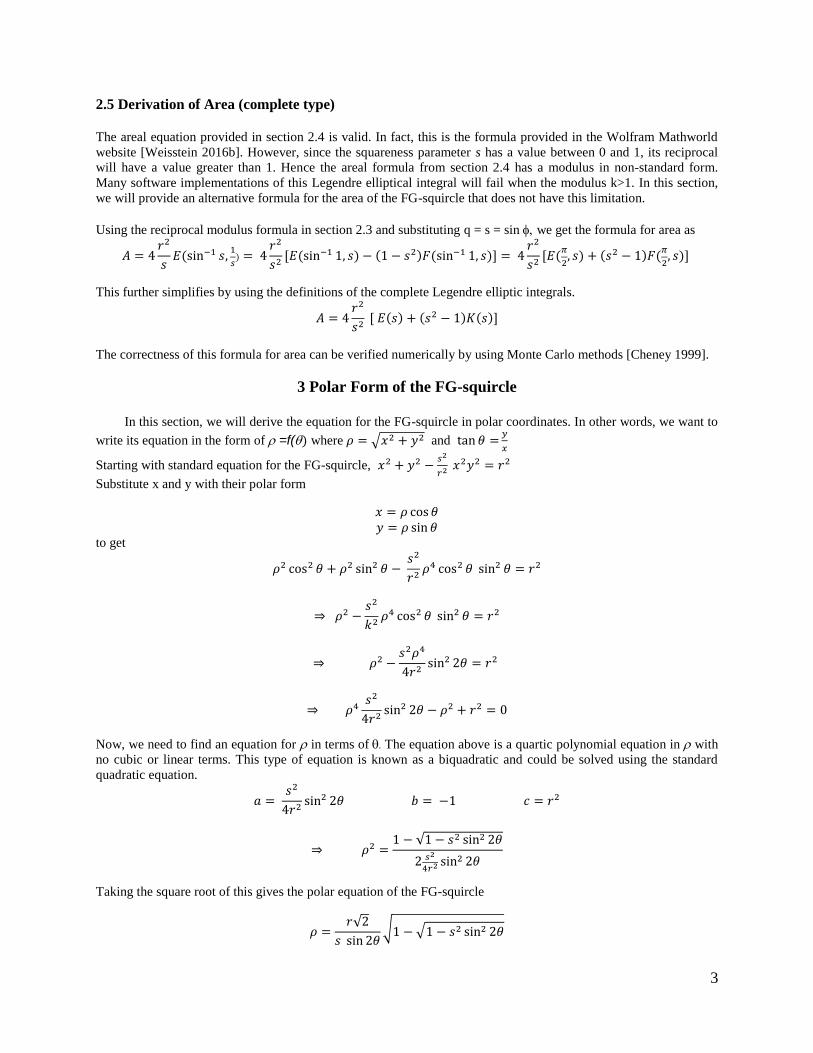
2.5 Derivation of Area (complete type)

The areal equation provided in section 2.4 is valid. In fact, this is the formula provided in the Wolfram Mathworld

website [Weisstein 2016b]. However, since the squareness parameter s has a value between 0 and 1, its reciprocal

will have a value greater than 1. Hence the areal formula from section 2.4 has a modulus in non-standard form.

Many software implementations of this Legendre elliptical integral will fail when the modulus k>1. In this section,

we will provide an alternative formula for the area of the FG-squircle that does not have this limitation.

Using the reciprocal modulus formula in section 2.3 and substituting q = s = sin we get the formula for area as

𝐴 = 4𝑟2

𝑠𝐸(sin−1 𝑠,

1

𝑠) = 4

𝑟2

𝑠2[𝐸(sin−1 1, 𝑠) − (1 − 𝑠2)𝐹(sin−1 1, 𝑠)] = 4

𝑟2

𝑠2[𝐸(

𝜋

2, 𝑠) + (𝑠2 − 1)𝐹(

𝜋

2, 𝑠)]

This further simplifies by using the definitions of the complete Legendre elliptic integrals.

𝐴 = 4𝑟2

𝑠2 [ 𝐸(𝑠) + (𝑠2 − 1)𝐾(𝑠)]

The correctness of this formula for area can be verified numerically by using Monte Carlo methods [Cheney 1999].

3 Polar Form of the FG-squircle

In this section, we will derive the equation for the FG-squircle in polar coordinates. In other words, we want to

write its equation in the form of =f() where 𝜌 = √𝑥2 + 𝑦2 and tan 𝜃 =𝑦

𝑥

Starting with standard equation for the FG-squircle, 𝑥2 + 𝑦2 −𝑠2

𝑟2 𝑥2𝑦2 = 𝑟2

Substitute x and y with their polar form

𝑥 = 𝜌 cos 𝜃

𝑦 = 𝜌 sin 𝜃 to get

𝜌2 cos2 𝜃 + 𝜌2 sin2 𝜃 − 𝑠2

𝑟2𝜌4 cos2 𝜃 sin2 𝜃 = 𝑟2

⇒ 𝜌2 −𝑠2

𝑘2𝜌4 cos2 𝜃 sin2 𝜃 = 𝑟2

⇒ 𝜌2 −𝑠2𝜌4

4𝑟2sin2 2𝜃 = 𝑟2

⇒ 𝜌4𝑠2

4𝑟2sin2 2𝜃 − 𝜌2 + 𝑟2 = 0

Now, we need to find an equation for in terms of The equation above is a quartic polynomial equation in with

no cubic or linear terms. This type of equation is known as a biquadratic and could be solved using the standard

quadratic equation.

𝑎 = 𝑠2

4𝑟2sin2 2𝜃 𝑏 = −1 𝑐 = 𝑟2

⇒ 𝜌2 =1 − √1 − 𝑠2 sin2 2𝜃

2 𝑠2

4𝑟2 sin2 2𝜃

Taking the square root of this gives the polar equation of the FG-squircle

𝜌 =𝑟√2

𝑠 sin 2𝜃√1 − √1 − 𝑠2 sin2 2𝜃

4

4 Parametric Equations for the FG-squircle

In this section, we present 3 sets of parametric equations for the FG-squircle. These equations are particularly useful

for plotting the FG-squircle. These equations can also be used in calculating the arc length of the FG-squircle,

which we will discuss in Section 5.2.

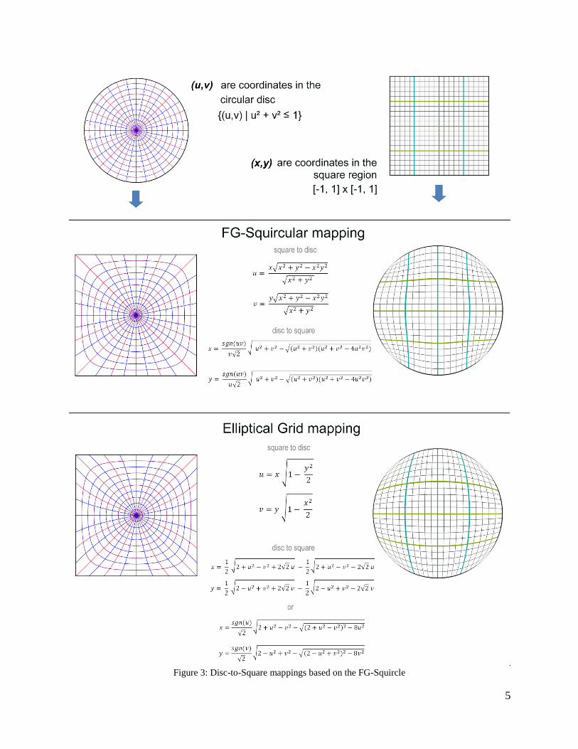
In 2014, Fong used a simplified FG-squircle to come up with two different methods to map the circle to a

square [Fong 2014a][Fong 2014b]. The two mappings are named the FG-squircular mapping and the elliptical grid

mapping, respectively and shown in Figure 3. The forward and inverse equations of the mappings are included in the

center column of the figure. Also, in order to illustrate the effects of the mapping, a circular disc with a radial grid is

converted to a square and shown in the left side of the figure. Similarly, a square region with a rectangular grid is

converted to a circular disc and shown in the right side of the figure.

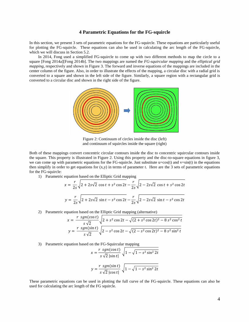
Figure 2: Continuum of circles inside the disc (left)

and continuum of squircles inside the square (right)

Both of these mappings convert concentric circular contours inside the disc to concentric squircular contours inside

the square. This property is illustrated in Figure 2. Using this property and the disc-to-square equations in figure 3,

we can come up with parametric equations for the FG-squircle. Just substitute u=cos(t) and v=sin(t) in the equations

then simplify in order to get equations for (x,y) in terms of parameter t. Here are the 3 sets of parametric equations

for the FG-squircle:

1) Parametric equation based on the Elliptic Grid mapping

𝑥 = 𝑟

2𝑠√2 + 2𝑠√2 cos 𝑡 + 𝑠2 cos 2𝑡 −

𝑟

2𝑠√2 − 2𝑠√2 cos 𝑡 + 𝑠2 cos 2𝑡

𝑦 = 𝑟

2𝑠√2 + 2𝑠√2 sin 𝑡 − 𝑠2 cos 2𝑡 −

𝑟

2𝑠√2 − 2𝑠√2 sin 𝑡 − 𝑠2 cos 2𝑡

2) Parametric equation based on the Elliptic Grid mapping (alternative)

𝑥 = 𝑟 𝑠𝑔𝑛(cos 𝑡)

𝑠 √2√2 + 𝑠2 cos 2𝑡 − √(2 + 𝑠2 cos 2𝑡)2 − 8 𝑠2 cos2 𝑡

𝑦 = 𝑟 𝑠𝑔𝑛(sin 𝑡)

𝑠 √2√2 − 𝑠2 cos 2𝑡 − √(2 − 𝑠2 cos 2𝑡)2 − 8 𝑠2 sin2 𝑡

3) Parametric equation based on the FG-Squircular mapping

𝑥 =𝑟 𝑠𝑔𝑛(cos 𝑡)

𝑠 √2 |sin 𝑡| √1 − √1 − 𝑠2 sin2 2𝑡

𝑦 =𝑟 𝑠𝑔𝑛(sin 𝑡)

𝑠 √2 |cos 𝑡| √1 − √1 − 𝑠2 sin2 2𝑡

These parametric equations can be used in plotting the full curve of the FG-squircle. These equations can also be

used for calculating the arc length of the FG squircle.

5

Figure 3: Disc-to-Square mappings based on the FG-Squircle

6

Using these parametric equations for the Fernandez Guasti squircle, we can easily get parametric equations for the

square by setting s=1. This square will have a side length of 2r.

1) Square parametric equation from Elliptic Grid mapping

𝑥 = 𝑟

2√2 + 2√2 cos 𝑡 + cos 2𝑡 −

𝑟

2√2 − 2√2 cos 𝑡 + cos 2𝑡

𝑦 = 𝑟

2√2 + 2√2 sin 𝑡 − cos 2𝑡 −

𝑟

2√2 − 2√2 sin 𝑡 − cos 2𝑡

2) Square parametric equation from Elliptic Grid mapping (alternative)

𝑥 = 𝑟 𝑠𝑔𝑛(cos 𝑡)

√2√2 + cos 2𝑡 − √(2 + cos 2𝑡)2 − 8 cos2 𝑡

𝑦 = 𝑟 𝑠𝑔𝑛(sin 𝑡)

√2√2 − cos 2𝑡 − √(2 − cos 2𝑡)2 − 8 sin2 𝑡

3) Square parametric equation from FG-Squircular mapping

𝑥 =𝑟 𝑠𝑔𝑛(cos 𝑡)

√2 |sin 𝑡| √1 − |cos 2𝑡|

𝑦 =𝑟 𝑠𝑔𝑛(sin 𝑡)

√2 |cos 𝑡| √1 − |cos 2𝑡|

5 Arc Length of the FG-squircle In this section, we shall provide three ways for calculating the arc length of the FG-squircle. Unfortunately, the

formulas we provide in this section are not closed-form analytical expressions. All of the arc length equations here

involve integrals that have to be calculated numerically to get an approximation of arc length.

5.1 Rectangular Cartesian coordinates y=f(x)

Given a curve with equation y=f(x), the formula for arc length in Cartesian coordinates is

𝑙 = ∫ √1 + [𝑓′(𝑥)]2 𝑑𝑥𝑥2

𝑥1

In order to use this formula for the FG-squircle, we need to convert the squircle equation to the form y=f(x). To do

this, we start with the standard equation for the FG-squircle: 𝑥2 + 𝑦2 −𝑠2

𝑟2 𝑥2𝑦2 = 𝑟2

Isolate y to one side of the equation, we get

𝑦2 = 𝑟2 − 𝑥2

1 −𝑠2

𝑟2 𝑥2

7

⇒ 𝑓(𝑥) = 𝑦 = √𝑟2 − 𝑥2

1 −𝑠2

𝑟2 𝑥2

Differentiating with respect to x, we get

𝑓′(𝑥) = 𝑠2𝑥 √𝑟2 − 𝑥2

𝑟2 (1 −𝑠2

𝑟2 𝑥2)

32

− 𝑥

√𝑟2 − 𝑥2√1 −𝑠2

𝑟2 𝑥2

which simplifies to

𝑓′(𝑥) = 𝑟3𝑥 (𝑠2 − 1)

√𝑟2 − 𝑥2(𝑟2 − 𝑠2𝑥2)32

Hence the incomplete arc length of the FG-squircle is

𝑙 = ∫ √1 +𝑟6𝑥2 (𝑠2 − 1)2

(𝑟2 − 𝑥2)(𝑟2 − 𝑠2𝑥2)3

𝑥2

𝑥1

𝑑𝑥

Unfortunately, we were unable to simplify this integral further. We even tried using computer algebra software with

symbolic math capabilities, but could not find a closed-form equation for the arc length of the FG-squircle.

However, this integral can be calculated numerically using standard techniques in numerical analysis.

5.2 Parametric formula for Arc Length

Given a curve with parametric equations for coordinates x(t) and y(t), the formula for arc length is

𝑙 = ∫ √(𝑑𝑥

𝑑𝑡)

2

+ (𝑑𝑦

𝑑𝑡)

2

𝑑𝑡𝑡2

𝑡1

One can then use any of the three parametric equations given in section 4 to plug into this to get an arc length

formula. This integral formula can then be numerically approximated.

5.3 Polar coordinates = f()

Another approach to computing the arc length of the FG-squircle is using polar coordinates. The equation for arc

length in polar coordinates is:

𝑙 = ∫ √𝜌2 + (𝑑𝜌

𝑑𝜃)

2

𝑑𝜃𝜃2

𝜃1

One can then use the polar form of the FG-squircle given in section 3 and plug into this equation to get an equation

for arc length which can then be numerically evaluated. For the complete arc length, simply use the limits of 0 to 2

𝑙𝑐𝑜𝑚𝑝𝑙𝑒𝑡𝑒 = ∫ √𝜌2 + (𝑑𝜌

𝑑𝜃)

2

𝑑𝜃2𝜋

0

8

6 Three Dimensional Counterpart of the FG-squircle

In this section, we present a three dimensional counterpart to the FG-squircle. The algebraic equation for this 3D

shape is

𝑥2 + 𝑦2 + 𝑧2 −𝑠2

𝑟2 𝑥2𝑦2 −

𝑠2

𝑟2 𝑦2𝑧2 −

𝑠2

𝑟2 𝑥2𝑧2 +

𝑠4

𝑟4𝑥2𝑦2𝑧2 = 𝑟2

Just like the FG-squircle, this shape has two parameters: squareness s and radius r. When s = 0, the shape is a sphere

with radius r. When s =1, the shape is a cube with side length 2r. In between, it is a three dimensional shape that

resembles the sphere and the cube. The shape is shown in figure 4 at varying values of squareness.

Figure 4: The 3D counterpart of the FG-squircle

We propose naming this shape as the sphube, which is a portmanteau of sphere and cube. This sort of naming would

be consistent with the naming of the squircle.

This algebraic shape is a sextic surface [Weisstein 2016a] because of the 𝑠4

𝑟4𝑥2𝑦2𝑧2 term. Just like in the FG-squircle,

we have limited the surface to (x,y,z) values such that -r ≤ x ≤ r and -r ≤ y ≤ r and -r ≤ z ≤ r.

7 Conjecture on a Four Dimensional Counterpart Since we were able to find a three dimensional counterpart of the FG-squircle in the previous section. We would like

to formulate a conjecture regarding the four dimensional counterpart of the FG-squircle in this section.

The four dimensional version of the sphere is known as the hypersphere (also 3-sphere). Similarly, the four

dimensional version of the cube is known as the hypercube (also tesseract). We conjecture that there is an algebraic

hypersurface that is an intermediate shape between these two four dimensional shapes. Moreover, we conjecture that

this hypersurface has the algebraic equation:

𝑥2 + 𝑦2 + 𝑧2 + 𝑤2 −𝑠2

𝑟2 𝑥2𝑦2 −

𝑠2

𝑟2 𝑦2𝑧2 −

𝑠2

𝑟2 𝑥2𝑧2 −

𝑠2

𝑟2 𝑥2𝑤2 −

𝑠2

𝑟2 𝑦2𝑤2 −

𝑠2

𝑟2 𝑧2𝑤2

+𝑠4

𝑟4𝑥2𝑦2𝑧2 +

𝑠4

𝑟4𝑥2𝑦2𝑤2 +

𝑠4

𝑟4𝑥2𝑧2𝑤2 +

𝑠4

𝑟4𝑦2𝑧2𝑤2 −

𝑠6

𝑟6𝑥2𝑦2𝑧2𝑤2 = 𝑟2

9

8 Summary In this paper, we provided several formulas related to the FG-squircle. We also presented a three dimensional

counterpart of the FG-squircle. The equations are summarized in the table below

Property Equation(s)

FG-Squircle 𝑥2 + 𝑦2 −

𝑠2

𝑟2 𝑥2𝑦2 = 𝑟2

Area (incomplete type) 𝐴 = 4

𝑟2

𝑠𝐸(sin−1 𝑠,

1

𝑠)

Area (complete type)

𝐴 = 4𝑟2

𝑠2 [ 𝐸(𝑠) + (𝑠2 − 1)𝐾(𝑠)]

Polar equation

𝜌 =𝑟√2

𝑠 sin 2𝜃√1 − √1 − 𝑠2 sin2 2𝜃

Parametric equation#1 𝑥 =

𝑟

2𝑠√2 + 2𝑠√2 cos 𝑡 + 𝑠2 cos 2𝑡 −

𝑟

2𝑠√2 − 2𝑠√2 cos 𝑡 + 𝑠2 cos 2𝑡

𝑦 = 𝑟

2𝑠√2 + 2𝑠√2 sin 𝑡 − 𝑠2 cos 2𝑡 −

𝑟

2𝑠√2 − 2𝑠√2 sin 𝑡 − 𝑠2 cos 2𝑡

Parametric equation#2 𝑥 =

𝑟 𝑠𝑔𝑛(cos 𝑡)

𝑠 √2√2 + 𝑠2 cos 2𝑡 − √(2 + 𝑠2 cos 2𝑡)2 − 8 𝑠2 cos2 𝑡

𝑦 = 𝑟 𝑠𝑔𝑛(sin 𝑡)

𝑠 √2√2 − 𝑠2 cos 2𝑡 − √(2 − 𝑠2 cos 2𝑡)2 − 8 𝑠2 sin2 𝑡

Parametric equation#3 𝑥 =

𝑟 𝑠𝑔𝑛(cos 𝑡)

𝑠 √2 |sin 𝑡| √1 − √1 − 𝑠2 sin2 2𝑡

𝑦 =𝑟 𝑠𝑔𝑛(sin 𝑡)

𝑠 √2 |cos 𝑡| √1 − √1 − 𝑠2 sin2 2𝑡

3D counterpart

𝑥2 + 𝑦2 + 𝑧2 −𝑠2

𝑟2 𝑥2𝑦2 −

𝑠2

𝑟2 𝑦2𝑧2 −

𝑠2

𝑟2 𝑥2𝑧2 +

𝑠4

𝑟4𝑥2𝑦2𝑧2 = 𝑟2

10

References Abramowitz, M., Stegun, I. 1972. “Handbook of Mathematical Functions” Dover. ISBN 0-486-61272-4 Cheney, W., Kincaid, D. 1999. “Numerical Mathematics and Computing (Fourth Edition)”. Brooks/Cole Publishing Company. ISBN 0-534-35184-0 Fernandez-Guasti, M. 1992. “Analytic Geometry of Some Rectilinear Figures” International Journal of Mathematical. Education in Science and Technology. 23, pp. 895-901 Fernandez-Guasti, M., Melendez-Cobarrubias, A., Renero-Carrillo, F., Cornejo-Rodriguez, A. 2005. “LCD pixel shape and far-field diffraction patterns”. Optik 116. Floater, M., Hormann, K. 2005. “Surface Parameterization: A Tutorial and Survey”. Advances in Multiresolution for Geometric Modelling. Fong, C., 2014. “An Indoor Alternative to Stereographic Spherical Panoramas”. Proceedings of Bridges 2014: Mathematics, Music, Art, Architecture, Culture. Fong, C., 2014. “Analytical Methods for Squaring the Disc”. Seoul International Congress of Mathematicians 2014. Nowell, P. “Mapping a Square to a Circle” (blog) http://mathproofs.blogspot.com/2005/07/mapping-square-to-circle.html Nowell, P. “Mapping a Cube to a Sphere” (blog) http://mathproofs.blogspot.com/2005/07/mapping-cube-to-sphere.html Weisstein, E. "Sextic Surface". MathWorld--A Wolfram Web Resource. http://mathworld.wolfram.com/SexticSurface.html Weisstein, E. "Squircle". MathWorld--A Wolfram Web Resource. http://mathworld.wolfram.com/Squircle.html