SPSS Workbook 1 Data Entry : Questionnaire Data Workbook 1 - Data... · 2 This workbook is designed...

1

TEESSIDE UNIVERSITY

SCHOOL OF HEALTH & SOCIAL CARE

SPSS Workbook 1 – Data Entry :

Questionnaire Data

Prepared by: Sylvia Storey [email protected]

SPSS – data entry

mailto:[email protected]

2

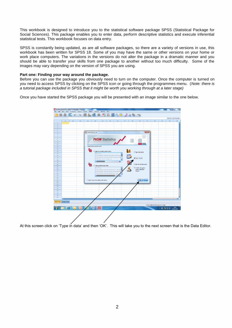
This workbook is designed to introduce you to the statistical software package SPSS (Statistical Package for Social Sciences). This package enables you to enter data, perform descriptive statistics and execute inferential statistical tests. This workbook focuses on data entry. SPSS is constantly being updated, as are all software packages, so there are a variety of versions in use, this workbook has been written for SPSS 18. Some of you may have the same or other versions on your home or work place computers. The variations in the versions do not alter the package in a dramatic manner and you should be able to transfer your skills from one package to another without too much difficulty. Some of the images may vary depending on the version of SPSS you are using. Part one: Finding your way around the package. Before you can use the package you obviously need to turn on the computer. Once the computer is turned on you need to access SPSS by clicking on the SPSS icon or going through the programmes menu. (Note: there is a tutorial package included in SPSS that it might be worth you working through at a later stage) Once you have started the SPSS package you will be presented with an image similar to the one below.

At this screen click on ‘Type in data’ and then ‘OK’. This will take you to the next screen that is the Data Editor.

3

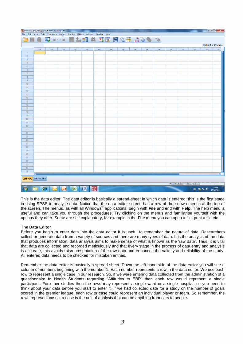
This is the data editor. The data editor is basically a spread-sheet in which data is entered; this is the first stage in using SPSS to analyse data. Notice that the data editor screen has a row of drop down menus at the top of the screen. The menus, as with all Windows

® applications, begin with File and end with Help. The help menu is

useful and can take you through the procedures. Try clicking on the menus and familiarise yourself with the options they offer. Some are self explanatory, for example in the File menu you can open a file, print a file etc. The Data Editor Before you begin to enter data into the data editor it is useful to remember the nature of data. Researchers collect or generate data from a variety of sources and there are many types of data. It is the analysis of the data that produces information; data analysis aims to make sense of what is known as the ‘raw data’. Thus, it is vital that data are collected and recorded meticulously and that every stage in the process of data entry and analysis is accurate, this avoids misrepresentation of the raw data and enhances the validity and reliability of the study. All entered data needs to be checked for mistaken entries. Remember the data editor is basically a spread-sheet. Down the left-hand side of the data editor you will see a column of numbers beginning with the number 1. Each number represents a row in the data editor. We use each row to represent a single case in our research. So, if we were entering data collected from the administration of a questionnaire to Health Students regarding “Attitudes to EBP” then each row would represent a single participant. For other studies then the rows may represent a single ward or a single hospital, so you need to think about your data before you start to enter it. If we had collected data for a study on the number of goals scored in the premier league, each row or case could represent an individual player or team. So remember, the rows represent cases, a case is the unit of analysis that can be anything from cars to people.

4

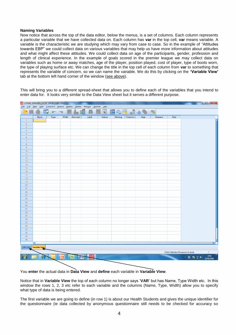
Naming Variables Now notice that across the top of the data editor, below the menus, is a set of columns. Each column represents a particular variable that we have collected data on. Each column has var in the top cell, var means variable. A variable is the characteristic we are studying which may vary from case to case. So in the example of “Attitudes towards EBP” we could collect data on various variables that may help us have more information about attitudes and what might affect these attitudes. We could collect data on age of the participants, gender, profession and length of clinical experience. In the example of goals scored in the premier league we may collect data on variables such as home or away matches, age of the player, position played, cost of player, type of boots worn, the type of playing surface etc. We can change the title in the top cell of each column from var to something that represents the variable of concern, so we can name the variable. We do this by clicking on the ‘Variable View’ tab at the bottom left hand corner of the window (see above). This will bring you to a different spread-sheet that allows you to define each of the variables that you intend to enter data for. It looks very similar to the Data View sheet but it serves a different purpose.

You enter the actual data in Data View and define each variable in Variable View. Notice that in Variable View the top of each column no longer says ‘VAR’ but has Name, Type Width etc. In this window the rows 1, 2, 3 etc refer to each variable and the columns (Name, Type, Width) allow you to specify what type of data is being entered. The first variable we are going to define (in row 1) is about our Health Students and gives the unique identifier for the questionnaire (ie data collected by anonymous questionnaire still needs to be checked for accuracy so

5

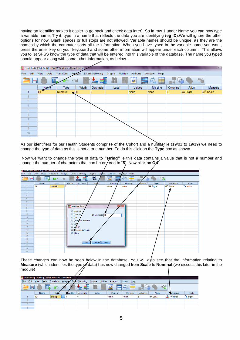
having an identifier makes it easier to go back and check data later). So in row 1 under Name you can now type a variable name. Try it, type in a name that reflects the data you are identifying (eg ID).We will ignore the other options for now. Blank spaces or full stops are not allowed. Variable names should be unique, as they are the names by which the computer sorts all the information. When you have typed in the variable name you want, press the enter key on your keyboard and some other information will appear under each column. This allows you to let SPSS know the type of data that will be entered into this variable of the database. The name you typed should appear along with some other information, as below.

As our identifiers for our Health Students comprise of the Cohort and a number ie (19/01 to 19/19) we need to change the type of data as this is not a true number. To do this click on the Type box as shown. Now we want to change the type of data to “string” ie this data contains a value that is not a number and change the number of characters that can be entered to “5”. Now click on OK

These changes can now be seen below in the database. You will also see that the information relating to Measure (which identifies the type of data) has now changed from Scale to Nominal (we discuss this later in the module)

6

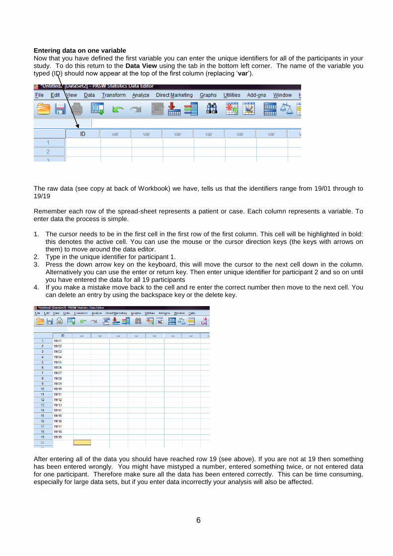
Entering data on one variable Now that you have defined the first variable you can enter the unique identifiers for all of the participants in your study. To do this return to the Data View using the tab in the bottom left corner. The name of the variable you typed (ID) should now appear at the top of the first column (replacing ‘var’).

The raw data (see copy at back of Workbook) we have, tells us that the identifiers range from 19/01 through to 19/19 Remember each row of the spread-sheet represents a patient or case. Each column represents a variable. To enter data the process is simple. 1. The cursor needs to be in the first cell in the first row of the first column. This cell will be highlighted in bold:

this denotes the active cell. You can use the mouse or the cursor direction keys (the keys with arrows on them) to move around the data editor.

2. Type in the unique identifier for participant 1. 3. Press the down arrow key on the keyboard, this will move the cursor to the next cell down in the column.

Alternatively you can use the enter or return key. Then enter unique identifier for participant 2 and so on until you have entered the data for all 19 participants

4. If you make a mistake move back to the cell and re enter the correct number then move to the next cell. You can delete an entry by using the backspace key or the delete key.

After entering all of the data you should have reached row 19 (see above). If you are not at 19 then something has been entered wrongly. You might have mistyped a number, entered something twice, or not entered data for one participant. Therefore make sure all the data has been entered correctly. This can be time consuming, especially for large data sets, but if you enter data incorrectly your analysis will also be affected.

7

We now want to define the rest of the variables that we will be using in our database – this means one variable for each piece of demographic information and every question on the questionnaire.

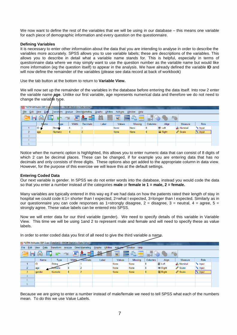
Defining Variables It is necessary to enter other information about the data that you are intending to analyse in order to describe the variables more accurately. SPSS allows you to use variable labels; these are descriptions of the variables. This allows you to describe in detail what a variable name stands for. This is helpful, especially in terms of questionnaire data where we may simply want to use the question number as the variable name but would like more information (eg the question itself) to appear in the analysis. We have already defined the variable ID and will now define the remainder of the variables (please see data record at back of workbook) Use the tab button at the bottom to return to Variable View. We will now set up the remainder of the variables in the database before entering the data itself. Into row 2 enter the variable name age. Unlike our first variable, age represents numerical data and therefore we do not need to change the variable type.

Notice when the numeric option is highlighted, this allows you to enter numeric data that can consist of 8 digits of which 2 can be decimal places. These can be changed, if for example you are entering data that has no decimals and only consists of three digits. These options also get added to the appropriate column in data view. However, for the purpose of this exercise we will leave this at the default settings. Entering Coded Data Our next variable is gender. In SPSS we do not enter words into the database, instead you would code the data so that you enter a number instead of the categories male or female ie 1 = male, 2 = female. Many variables are typically entered in this way eg if we had data on how the patients rated their length of stay in hospital we could code it:1= shorter than I expected, 2=what I expected, 3=longer than I expected. Similarly as in our questionnaire you can code responses as 1=strongly disagree, 2 = disagree, 3 = neutral, 4 = agree, 5 = strongly agree. These value labels can be entered into SPSS. Now we will enter data for our third variable (gender). We need to specify details of this variable in Variable View. This time we will be using 1and 2 to represent male and female and will need to specify these as value labels. In order to enter coded data you first of all need to give the third variable a name.

Because we are going to enter a number instead of male/female we need to tell SPSS what each of the numbers mean. To do this we use Value Labels.

8

Value Labels 1. In the Variable View spread sheet you need to define value labels. Make sure you stay on Row 3 (our

variable for gender) and go to the cell under the column headed ‘Values’, and click on the little grey box (with 3 dots) this will bring up the window below:

2. Place the cursor in the box “Value” and type in the number one. 3. Place the cursor in the box “Label” and type in male.

4. Click on “Add” you should see that 1 equates with male in the lower box. Repeat this for the other values. (2=female)

Again click on Add and then select OK and you will see that the 2 values are now in the box. Click on OK

9

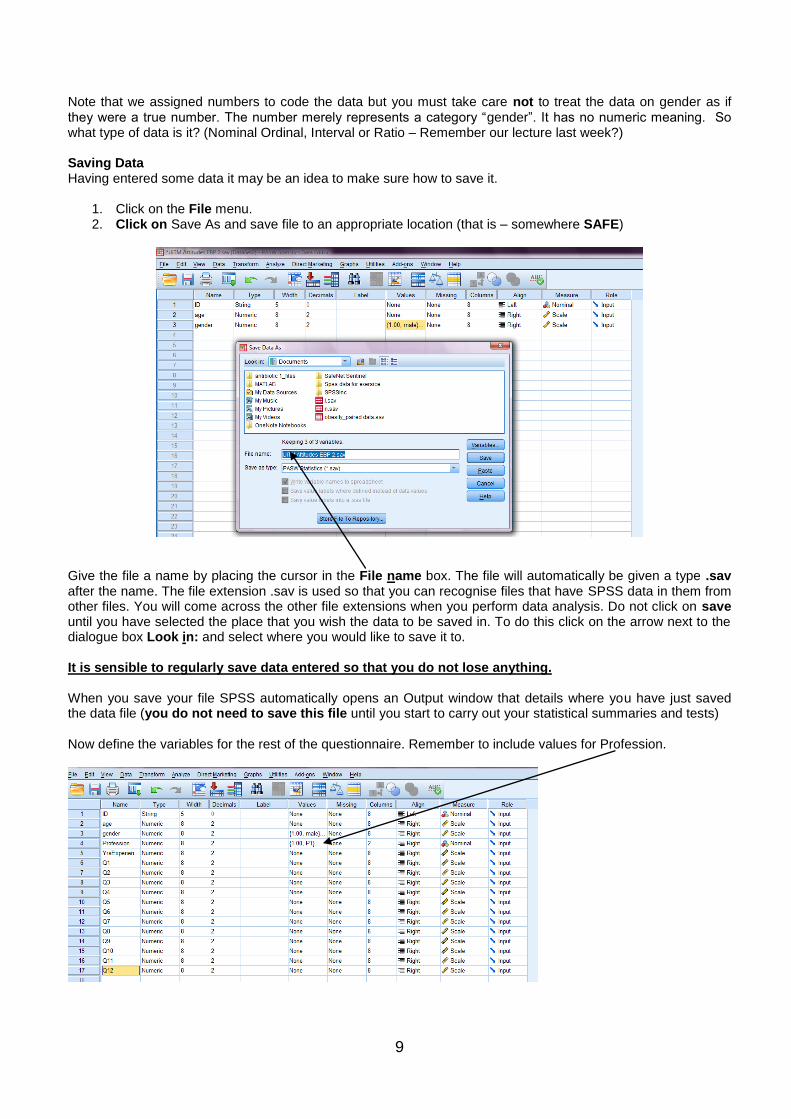
Note that we assigned numbers to code the data but you must take care not to treat the data on gender as if they were a true number. The number merely represents a category “gender”. It has no numeric meaning. So what type of data is it? (Nominal Ordinal, Interval or Ratio – Remember our lecture last week?) Saving Data Having entered some data it may be an idea to make sure how to save it.

1. Click on the File menu. 2. Click on Save As and save file to an appropriate location (that is – somewhere SAFE)

Give the file a name by placing the cursor in the File name box. The file will automatically be given a type .sav after the name. The file extension .sav is used so that you can recognise files that have SPSS data in them from other files. You will come across the other file extensions when you perform data analysis. Do not click on save until you have selected the place that you wish the data to be saved in. To do this click on the arrow next to the dialogue box Look in: and select where you would like to save it to. It is sensible to regularly save data entered so that you do not lose anything. When you save your file SPSS automatically opens an Output window that details where you have just saved the data file (you do not need to save this file until you start to carry out your statistical summaries and tests) Now define the variables for the rest of the questionnaire. Remember to include values for Profession.

10

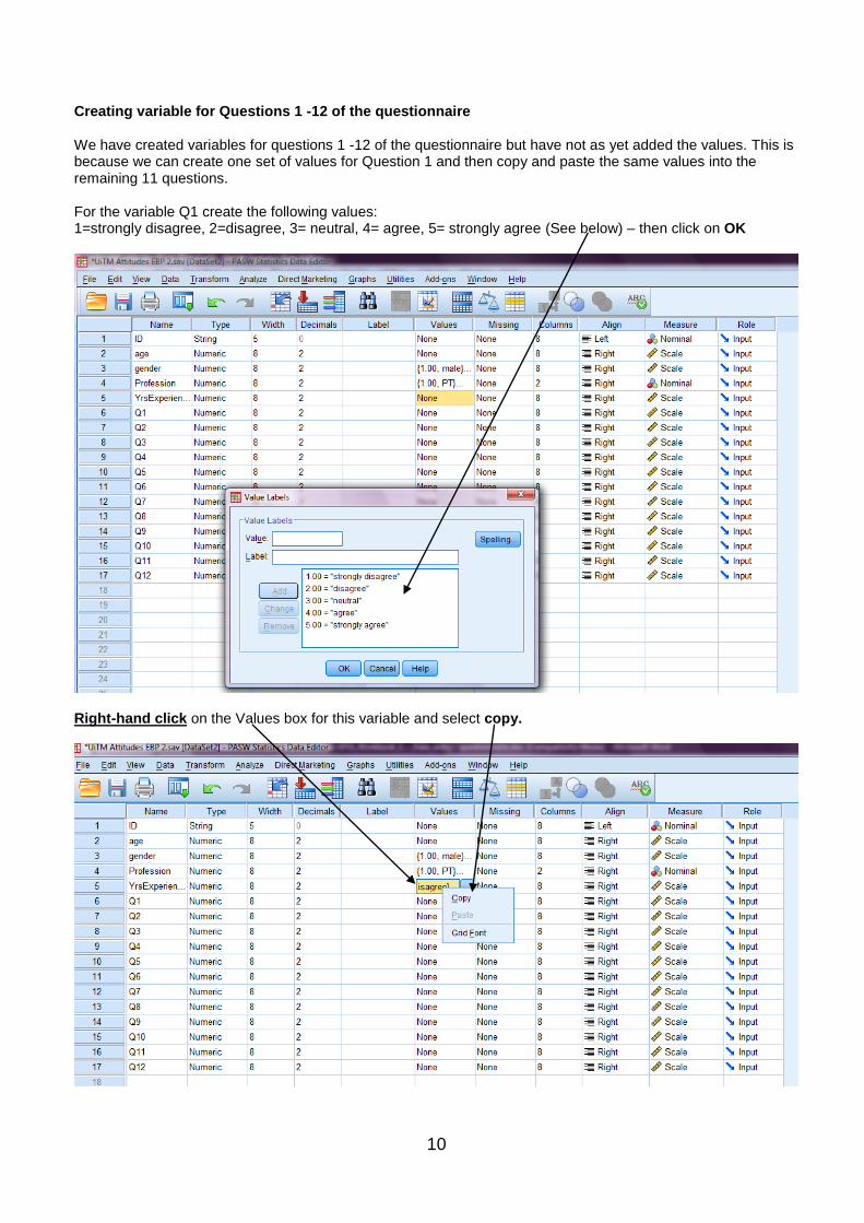
Creating variable for Questions 1 -12 of the questionnaire We have created variables for questions 1 -12 of the questionnaire but have not as yet added the values. This is because we can create one set of values for Question 1 and then copy and paste the same values into the remaining 11 questions. For the variable Q1 create the following values: 1=strongly disagree, 2=disagree, 3= neutral, 4= agree, 5= strongly agree (See below) – then click on OK

Right-hand click on the Values box for this variable and select copy.

11

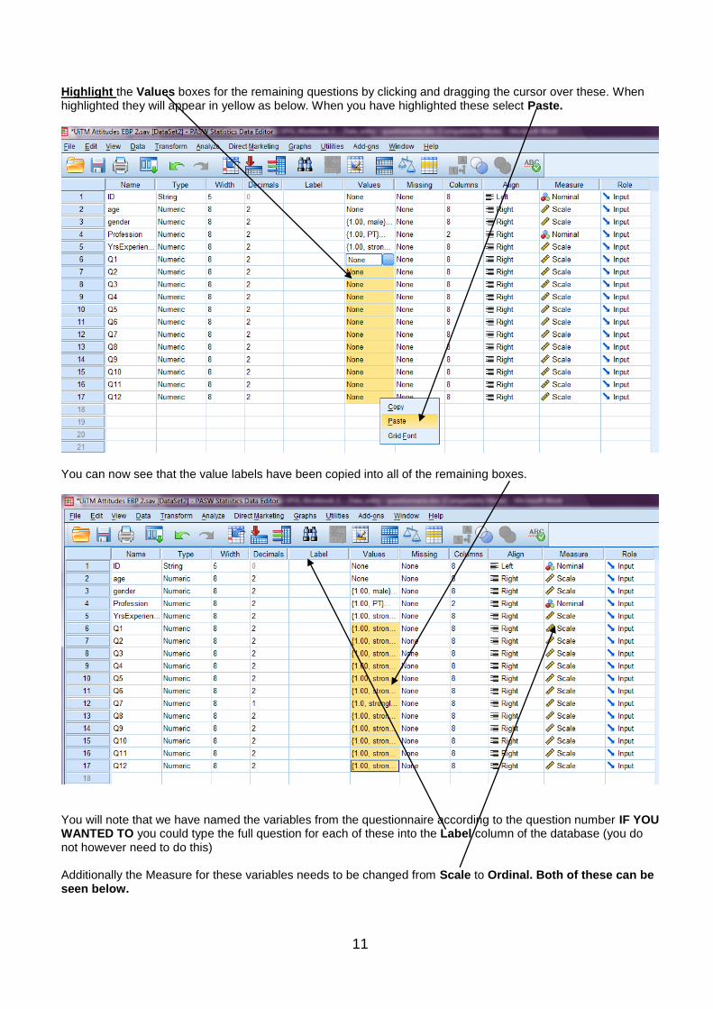
Highlight the Values boxes for the remaining questions by clicking and dragging the cursor over these. When highlighted they will appear in yellow as below. When you have highlighted these select Paste.

You can now see that the value labels have been copied into all of the remaining boxes.

You will note that we have named the variables from the questionnaire according to the question number IF YOU WANTED TO you could type the full question for each of these into the Label column of the database (you do not however need to do this) Additionally the Measure for these variables needs to be changed from Scale to Ordinal. Both of these can be seen below.

12

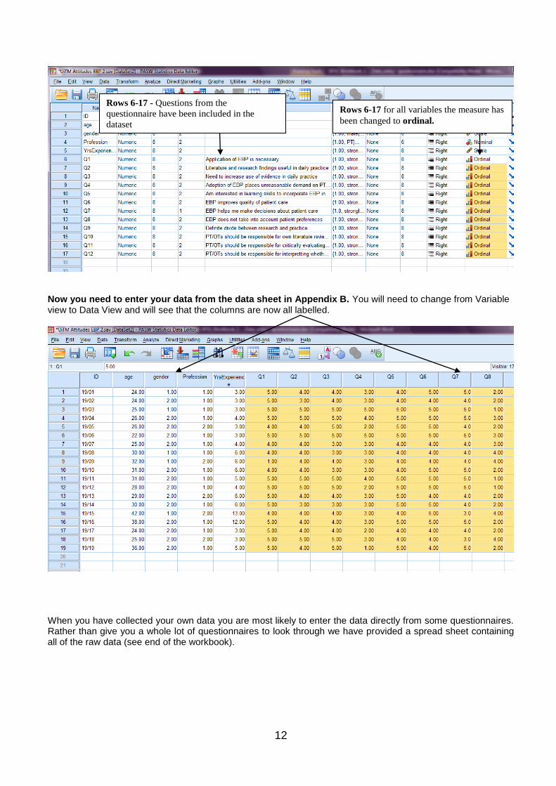
Now you need to enter your data from the data sheet in Appendix B. You will need to change from Variable view to Data View and will see that the columns are now all labelled.

When you have collected your own data you are most likely to enter the data directly from some questionnaires. Rather than give you a whole lot of questionnaires to look through we have provided a spread sheet containing all of the raw data (see end of the workbook).

Rows 6-17 - Questions from the

questionnaire have been included in the

dataset

Rows 6-17 for all variables the measure has

been changed to ordinal.

13

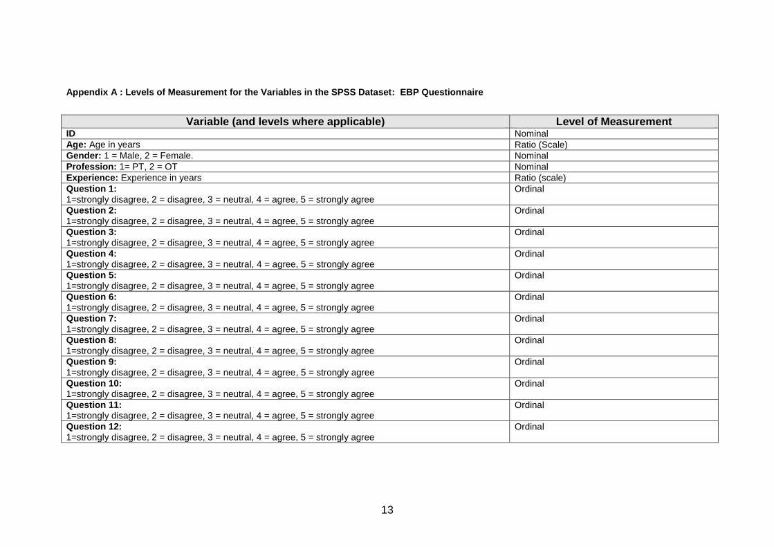
Appendix A : Levels of Measurement for the Variables in the SPSS Dataset: EBP Questionnaire

Variable (and levels where applicable) Level of Measurement ID Nominal

Age: Age in years Ratio (Scale)

Gender: 1 = Male, 2 = Female. Nominal

Profession: 1= PT, 2 = OT Nominal

Experience: Experience in years Ratio (scale)

Question 1: 1=strongly disagree, 2 = disagree, 3 = neutral, 4 = agree, 5 = strongly agree

Ordinal


Ordinal


Ordinal


Ordinal


Ordinal


Ordinal


Ordinal


Ordinal


Ordinal


Ordinal


Ordinal


Ordinal

14

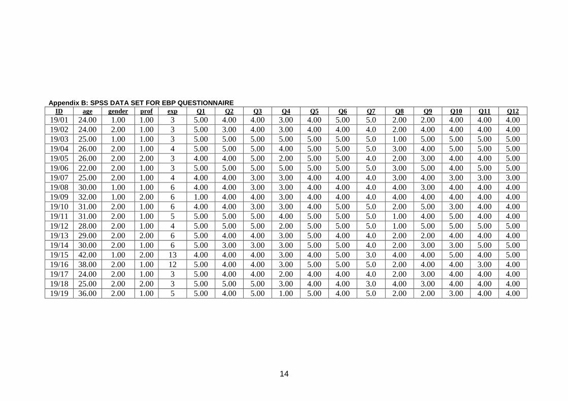
Appendix B: SPSS DATA SET FOR EBP QUESTIONNAIRE

ID age gender prof exp Q1 Q2 Q3 Q4 Q5 Q6 Q7 Q8 Q9 Q10 Q11 Q12

19/01 24.00 1.00 1.00 3 5.00 4.00 4.00 3.00 4.00 5.00 5.0 2.00 2.00 4.00 4.00 4.00

19/02 24.00 2.00 1.00 3 5.00 3.00 4.00 3.00 4.00 4.00 4.0 2.00 4.00 4.00 4.00 4.00

19/03 25.00 1.00 1.00 3 5.00 5.00 5.00 5.00 5.00 5.00 5.0 1.00 5.00 5.00 5.00 5.00

19/04 26.00 2.00 1.00 4 5.00 5.00 5.00 4.00 5.00 5.00 5.0 3.00 4.00 5.00 5.00 5.00

19/05 26.00 2.00 2.00 3 4.00 4.00 5.00 2.00 5.00 5.00 4.0 2.00 3.00 4.00 4.00 5.00

19/06 22.00 2.00 1.00 3 5.00 5.00 5.00 5.00 5.00 5.00 5.0 3.00 5.00 4.00 5.00 5.00

19/07 25.00 2.00 1.00 4 4.00 4.00 3.00 3.00 4.00 4.00 4.0 3.00 4.00 3.00 3.00 3.00

19/08 30.00 1.00 1.00 6 4.00 4.00 3.00 3.00 4.00 4.00 4.0 4.00 3.00 4.00 4.00 4.00

19/09 32.00 1.00 2.00 6 1.00 4.00 4.00 3.00 4.00 4.00 4.0 4.00 4.00 4.00 4.00 4.00

19/10 31.00 2.00 1.00 6 4.00 4.00 3.00 3.00 4.00 5.00 5.0 2.00 5.00 3.00 4.00 4.00

19/11 31.00 2.00 1.00 5 5.00 5.00 5.00 4.00 5.00 5.00 5.0 1.00 4.00 5.00 4.00 4.00

19/12 28.00 2.00 1.00 4 5.00 5.00 5.00 2.00 5.00 5.00 5.0 1.00 5.00 5.00 5.00 5.00

19/13 29.00 2.00 2.00 6 5.00 4.00 4.00 3.00 5.00 4.00 4.0 2.00 2.00 4.00 4.00 4.00

19/14 30.00 2.00 1.00 6 5.00 3.00 3.00 3.00 5.00 5.00 4.0 2.00 3.00 3.00 5.00 5.00

19/15 42.00 1.00 2.00 13 4.00 4.00 4.00 3.00 4.00 5.00 3.0 4.00 4.00 5.00 4.00 5.00

19/16 38.00 2.00 1.00 12 5.00 4.00 4.00 3.00 5.00 5.00 5.0 2.00 4.00 4.00 3.00 4.00

19/17 24.00 2.00 1.00 3 5.00 4.00 4.00 2.00 4.00 4.00 4.0 2.00 3.00 4.00 4.00 4.00

19/18 25.00 2.00 2.00 3 5.00 5.00 5.00 3.00 4.00 4.00 3.0 4.00 3.00 4.00 4.00 4.00

19/19 36.00 2.00 1.00 5 5.00 4.00 5.00 1.00 5.00 4.00 5.0 2.00 2.00 3.00 4.00 4.00

SPSS Workbook 1 Data Entry : Questionnaire Data Workbook 1 - Data... · 2 This workbook is designed...

Documents

Transcript of SPSS Workbook 1 Data Entry : Questionnaire Data Workbook 1 - Data... · 2 This workbook is designed...