SPSS Tables 11 - LUpriede.bf.lu.lv/grozs/Datorlietas/SPSS/SPSS Tables 11.5.pdf · manual, is also...
260
SPSS Tables ™ 11.5
Transcript of SPSS Tables 11 - LUpriede.bf.lu.lv/grozs/Datorlietas/SPSS/SPSS Tables 11.5.pdf · manual, is also...

SPSS Tables™ 11.5

For more information about SPSS® software products, please visit our Web site at http://www.spss.com, orcontact:
SPSS Inc.233 South Wacker Drive, 11th FloorChicago, IL 60606-6412Tel: (312) 651-3000Fax: (312) 651-3668
SPSS is a registered trademark and the other product names are the trademarks of SPSS Inc. for its proprietary computer software. No material describing such software may be produced or distributed without the written permission of the owners of the trademark and license rights in the software and the copyrights in the published materials.
The SOFTWARE and documentation are provided with RESTRICTED RIGHTS. Use, duplication, or disclosure by the Government is subject to restrictions as set forth in subdivision (c)(1)(ii) of The Rights in Technical Data and Computer Software clause at 52.227-7013. Contractor/manufacturer is SPSS Inc., 233 South Wacker Drive, 11th Floor, Chicago, IL 60606-6412.
General notice: Other product names mentioned herein are used for identification purposes only and may be trademarks of their respective companies.
TableLook is a trademark of SPSS Inc.Windows is a registered trademark of Microsoft Corporation.DataDirect, DataDirect Connect, INTERSOLV, and SequeLink are registered trademarks of MERANT Solutions Inc.Portions of this product were created using LEADTOOLS © 1991–2000, LEAD Technologies, Inc. ALL RIGHTS RESERVED. LEAD, LEADTOOLS, and LEADVIEW are registered trademarks of LEAD Technologies, Inc.Portions of this product were based on the work of the FreeType Team (http://www.freetype.org).
SPSS Tables™ 11.5Copyright © 2002 by SPSS Inc.All rights reserved.Printed in the United States of America.
No part of this publication may be reproduced, stored in a retrieval system, or transmitted, in any form or by any means, electronic, mechanical, photocopying, recording, or otherwise, without the prior written permission of the publisher.
2 3 4 5 6 7 8 9 0 06 05 04 03
ISBN 1-56827-302-9
iii
P r e f a c e
SPSS® 11.5 is a comprehensive system for analyzing data. SPSS can take data from almost any type of file and use them to generate tabulated reports, charts, and plots of distributions and trends, descriptive statistics, and complex statistical analyses.
The Tables option is an add-on enhancement that enables you to prepare customized tables suitable for presentation or publication. Through Tables, you can access a wide variety of descriptive statistics and can combine large amounts of information in a single display. The Tables option must be used with the SPSS 11.5 Base and is completely integrated into that system.
Professionals in many different fields will find the Tables procedure beneficial. People in business, for example, can use Tables for periodic status reports and for analyses that support decision making. Market researchers and survey researchers can use Tables to meet the tabular style requirements of academic institutions or professional journals. The flexibility of Tables allows you to follow a prescribed style or, if you choose, design your own.
About This Manual
This manual provides a guide to the Tables option and describes how to obtain the appropriate tables using the dialog box interface. It also gives an item-by-item description of each dialog box. The Tables command syntax, found near the end of the manual, is also included in the SPSS 11.5 Syntax Reference Guide, available on the product CD-ROM.
This manual contains two indexes: a subject index and a syntax index. The subject index covers the entire manual. The syntax index applies only to the syntax reference material.
Installation
To install Tables, follow the instructions for adding and removing features in the installation instructions supplied with the SPSS Base. (To start, double-click on the SPSS setup icon.)
iv
Compatibility
The SPSS system is designed to operate on many computer systems. See the installation instructions that came with your system for specific information on minimum and recommended requirements.
Serial Numbers
Your serial number is your identification number with SPSS Inc. You will need this serial number when you contact SPSS Inc. for information regarding support, payment, or an upgraded system. The serial number was provided with your Base system. Before using the system, please copy this number to the registration card.
Registration Card
Don’t put it off: fill out and send us your registration card. Until we receive your registration card, you have an unregistered system. Even if you have previously sent a card to us, please fill out and return the card enclosed in your Tables package. Registering your system entitles you to:
� Technical support services
� New product announcements and upgrade announcements
Customer Service
If you have any questions concerning your shipment or account, contact your local office, listed on page vi. Please have your serial number ready for identification when calling.
Training Seminars
SPSS Inc. provides both public and onsite training seminars for SPSS. All seminars feature hands-on workshops. SPSS seminars will be offered in major U.S. and European cities on a regular basis. For more information about these seminars, call your local office, listed on page vi.

v
Technical Support
The services of SPSS Technical Support are available to registered customers of SPSS. Customers may contact Technical Support for assistance in using SPSS products or for installation help for one of the supported hardware environments. To reach Technical Support, see the SPSS Web site at http://www.spss.com or call your local office, listed on page vi. Be prepared to identify yourself, your organization, and the serial number of your system.
Additional Publications
Except for academic course adoptions, additional copies of SPSS product manuals may be purchased directly from SPSS Inc. Visit our Web site at http://www.spss.com/estore, or contact your local SPSS office, listed on page vi.
SPSS product manuals may also be purchased from Prentice Hall, the exclusive distributor of SPSS publications. To order, fill out and mail the Publications order form included with your system, or call 800-947-7700. If you represent a bookstore or have an account with Prentice Hall, call 800-382-3419. In Canada, call 800-567-3800. Outside of North America, contact your local Prentice Hall office.
Statistical introductions to procedures in the Base, Regression Models, and Advanced Models written by Marija Norusis are planned to be available from Prentice Hall. Check with the publisher or visit the SPSS Web site for announcements regarding availability.
Tell Us Your Thoughts
Your comments are important. Please let us know about your experiences with SPSS products. We especially like to hear about new and interesting applications using the SPSS system. Please send e-mail to [email protected], or write to SPSS Inc., Attn: Director of Product Planning, 233 South Wacker Drive, 11th Floor, Chicago, IL 60606-6412.
Contacting SPSS
If you would like to be on our mailing list, contact one of our offices, listed on page vi, or visit our Web site at http://www.spss.com. We will send you a copy of our newsletter and let you know about SPSS Inc. activities in your area.
v

vi
SPSS Inc.Chicago, Illinois, U.S.A.Tel: 1.312.651.3000or 1.800.543.2185www.spss.com/corpinfoCustomer Service:1.800.521.1337Sales:[email protected]: 1.800.543.6607Technical Support:[email protected]
SPSS Federal SystemsTel: 1.703.740.2400or 1.800.860.5762www.spss.com
SPSS AndinoTel: +57.1.635.8585www.spss.com/la
SPSS Argentina SATel: +5411.4371.5031www.spss.com/la
SPSS Asia Pacific Pte. Ltd.Tel: +65.245.9110www.spss.com
SPSS Australasia Pty. Ltd.Tel: +61.2.9954.5660www.spss.com
SPSS BelgiumTel: +32.163.170.70www.spss.com
SPSS Benelux BVTel: +31.183.651777www.spss.com
SPSS Brasil Ltda.Tel: +55.11.5505.3644www.spss.com
SPSS ChileTel: +56.2.233.7499www.spss.com/la
SPSS Czech RepublicTel: +420.2.24813839www.spss.cz
SPSS DenmarkTel: +45.45.46.02.00www.spss.com
SPSS East Africa Tel: +254 2 577 262spss.com
SPSS Finland OyTel: +358.9.4355.920www.spss.com
SPSS France SARLTel: +01.55.35.27.00 www.spss.com
SPSS Germany Tel: +49.89.4890740www.spss.com
SPSS BI GreeceTel: +30.1.6971950www.spss.com
SPSS Iberica, S.L.U.Tel: +34.902.123.606SPSS.com
SPSS Hong Kong Ltd.Tel: +852.2.811.9662www.spss.com
SPSS IrelandTel: +353.1.415.0234www.spss.com
SPSS BI IsraelTel: +972.3.6166616www.spss.com
SPSS Italia srlTel: +800.437300www.spss.it
SPSS Japan Inc.Tel: +81.3.5466.5511www.spss.co.jp
SPSS Korea DataSolution Co.Tel: +82.2.563.0014www.spss.co.kr
SPSS Latin AmericaTel: +1.312.651.3539www.spss.com
SPSS Malaysia Sdn BhdTel: +603.6203.2300www.spss.com
SPSS MiamiTel: 1.305.627.5700SPSS.com
SPSS Mexico SA de CV Tel: +52.5.682.87.68www.spss.com
SPSS Norway ASTel: +47.22.99.25.50www.spss.com
SPSS PolskaTel: +48.12.6369680www.spss.pl
SPSS RussiaTel: +7.095.125.0069www.spss.com
SPSS San BrunoTel: 1.650.794.2692www.spss.com
SPSS Schweiz AGTel: +41.1.266.90.30www.spss.com
SPSS BI (Singapore) Pte. Ltd.Tel: +65.346.2061www.spss.com
SPSS South Africa Tel: +27.21.7120929www.spss.com
SPSS South AsiaTel: +91.80.2088069www.spss.com
SPSS Sweden ABTel: +46.8.506.105.50www.spss.com
SPSS Taiwan Corp.Taipei, Republic of ChinaTel: +886.2.25771100www.sinter.com.tw/spss/main
SPSS (Thailand) Co., Ltd.Tel: +66.2.260.7070www.spss.com
SPSS UK Ltd.Tel: +44.1483.719200www.spss.com

vii
C o n t e n t s
1 Getting Started with SPSS Tables 1
What’s New in Tables? . . . . . . . . . . . . . . . . . . . . . . . . . . . . . 1
Table Structure and Terminology . . . . . . . . . . . . . . . . . . . . . . . 2
Pivot Tables . . . . . . . . . . . . . . . . . . . . . . . . . . . . . . . . . 2Variables and Level of Measurement . . . . . . . . . . . . . . . . . . 3Rows, Columns, and Cells . . . . . . . . . . . . . . . . . . . . . . . . . 4Stacking . . . . . . . . . . . . . . . . . . . . . . . . . . . . . . . . . . . 4Crosstabulation . . . . . . . . . . . . . . . . . . . . . . . . . . . . . . . 5Nesting . . . . . . . . . . . . . . . . . . . . . . . . . . . . . . . . . . . . 5Layers . . . . . . . . . . . . . . . . . . . . . . . . . . . . . . . . . . . . 6
Tables for Variables with Shared Categories . . . . . . . . . . . . . . . . . 7
Multiple Response Sets . . . . . . . . . . . . . . . . . . . . . . . . . . . . . 7
Totals and Subtotals . . . . . . . . . . . . . . . . . . . . . . . . . . . . . . . 8
Custom Summary Statistics for Totals . . . . . . . . . . . . . . . . . . 9Sample Data File . . . . . . . . . . . . . . . . . . . . . . . . . . . . . . . . 10
Building a Table . . . . . . . . . . . . . . . . . . . . . . . . . . . . . . . . 10
Opening the Custom Table Builder . . . . . . . . . . . . . . . . . . . 11Selecting Row and Column Variables . . . . . . . . . . . . . . . . . 13Inserting Totals and Subtotals . . . . . . . . . . . . . . . . . . . . . 16Summarizing Scale Variables . . . . . . . . . . . . . . . . . . . . . . 19
2 Table Builder Interface 25
Building Tables . . . . . . . . . . . . . . . . . . . . . . . . . . . . . . . . . 26
To Build a Table . . . . . . . . . . . . . . . . . . . . . . . . . . . . . . 29Stacking Variables . . . . . . . . . . . . . . . . . . . . . . . . . . . . 29Nesting Variables . . . . . . . . . . . . . . . . . . . . . . . . . . . . . 30Layers . . . . . . . . . . . . . . . . . . . . . . . . . . . . . . . . . . . 32

viii
Showing and Hiding Variable Names and/or Labels . . . . . . . . . 33Summary Statistics . . . . . . . . . . . . . . . . . . . . . . . . . . . . 33Categories and Totals . . . . . . . . . . . . . . . . . . . . . . . . . . 42Tables of Variables with Shared Categories (Comperimeter Tables) . . . . . . . . . . . . . . . . . . . . . . . . . . 47Customizing the Table Builder . . . . . . . . . . . . . . . . . . . . . 48
Custom Tables: Options Tab . . . . . . . . . . . . . . . . . . . . . . . . . 48
Custom Tables: Titles Tab . . . . . . . . . . . . . . . . . . . . . . . . . . . 51
Custom Tables: Test Statistics Tab . . . . . . . . . . . . . . . . . . . . . 52
3 Simple Tables for Categorical Variables 55
A Single Categorical Variable . . . . . . . . . . . . . . . . . . . . . . . . 56
Percentages. . . . . . . . . . . . . . . . . . . . . . . . . . . . . . . . 57Totals . . . . . . . . . . . . . . . . . . . . . . . . . . . . . . . . . . . . 59
Crosstabulation. . . . . . . . . . . . . . . . . . . . . . . . . . . . . . . . . 61
Percentages in Crosstabulations . . . . . . . . . . . . . . . . . . . . 62Controlling Display Format. . . . . . . . . . . . . . . . . . . . . . . . 63Marginal Totals . . . . . . . . . . . . . . . . . . . . . . . . . . . . . . 64
Sorting and Excluding Categories . . . . . . . . . . . . . . . . . . . . . . 66
4 Stacking, Nesting, and Layers with Categorical Variables 73
Stacking Categorical Variables. . . . . . . . . . . . . . . . . . . . . . . . 73
Stacking with Crosstabulation . . . . . . . . . . . . . . . . . . . . . 75Nesting Categorical Variables . . . . . . . . . . . . . . . . . . . . . . . . 76
Suppressing Variable Labels . . . . . . . . . . . . . . . . . . . . . . 79Nested Crosstabulation . . . . . . . . . . . . . . . . . . . . . . . . . 81
Layers . . . . . . . . . . . . . . . . . . . . . . . . . . . . . . . . . . . . . . 84
Two Stacked Categorical Layer Variables. . . . . . . . . . . . . . . 87Two Nested Categorical Layer Variables . . . . . . . . . . . . . . . 88

ix
5 Totals and Subtotals for Categorical Variables 91
Simple Total for a Single Variable. . . . . . . . . . . . . . . . . . . . . . .91
What You See Is What Gets Totaled . . . . . . . . . . . . . . . . . .93Display Position of Totals . . . . . . . . . . . . . . . . . . . . . . . . .95Totals for Nested Tables . . . . . . . . . . . . . . . . . . . . . . . . .95Layer Variable Totals . . . . . . . . . . . . . . . . . . . . . . . . . . .98
Subtotals . . . . . . . . . . . . . . . . . . . . . . . . . . . . . . . . . . . . .99
What You See Is What Gets Subtotaled . . . . . . . . . . . . . . . 101Layer Variable Subtotals . . . . . . . . . . . . . . . . . . . . . . . . 102
6 Tables for Variables with Shared Categories 103
Table of Counts . . . . . . . . . . . . . . . . . . . . . . . . . . . . . . . . 104
Table of Percentages . . . . . . . . . . . . . . . . . . . . . . . . . . . . . 106
Totals and Category Control . . . . . . . . . . . . . . . . . . . . . . . . . 108
Nesting in Tables with Shared Categories . . . . . . . . . . . . . . . . . 111
7 Summary Statistics 113
Summary Statistics Source Variable . . . . . . . . . . . . . . . . . . . . 114
Summary Statistics Source for Categorical Variables . . . . . . . 115Summary Statistics Source for Scale Variables . . . . . . . . . . . 118
Stacked Variables . . . . . . . . . . . . . . . . . . . . . . . . . . . . . . . 121
Custom Total Summary Statistics for Categorical Variables. . . . . . . 124
Displaying Category Values . . . . . . . . . . . . . . . . . . . . . . 128
x
8 Summarizing Scale Variables 131
Stacked Scale Variables . . . . . . . . . . . . . . . . . . . . . . . . . . 132
Multiple Summary Statistics . . . . . . . . . . . . . . . . . . . . . . . . 133
Count, Valid N, and Missing Values . . . . . . . . . . . . . . . . . . . . 134
Different Summaries for Different Variables . . . . . . . . . . . . . . . 136
Group Summaries in Categories . . . . . . . . . . . . . . . . . . . . . . 139
Multiple Grouping Variables. . . . . . . . . . . . . . . . . . . . . . 139Nesting Categorical Variables within Scale Variables. . . . . . . 142
9 Test Statistics 145
Tests of Independence (Chi-Square) . . . . . . . . . . . . . . . . . . . 145
Effects of Nesting and Stacking on Tests of Independence. . . . 150Comparing Column Means . . . . . . . . . . . . . . . . . . . . . . . . . 152
Effects of Nesting and Stacking on Column Means Tests . . . . . 155Comparing Column Proportions . . . . . . . . . . . . . . . . . . . . . . 158
Effects of Nesting and Stacking on Column Proportions Tests . . 162
10 Multiple Response Sets 167
Defining Multiple Response Sets. . . . . . . . . . . . . . . . . . . . . . 168
Counts, Responses, Percentages, and Totals . . . . . . . . . . . . . . 170
Using Multiple Response Sets with Other Variables . . . . . . . . . . 174
Statistics Source Variable and Available Summary Statistics . . 176Multiple Category Sets and Duplicate Responses . . . . . . . . . . . . 178

xi
11 Missing Values 181
Tables without Missing Values . . . . . . . . . . . . . . . . . . . . . . . 182
Including Missing Values in Tables . . . . . . . . . . . . . . . . . . . . . 184
12 Formatting and Customizing Tables 187
Summary Statistics Display Format . . . . . . . . . . . . . . . . . . . . . 188
Display Labels for Summary Statistics . . . . . . . . . . . . . . . . . . . 192
Column Width . . . . . . . . . . . . . . . . . . . . . . . . . . . . . . . . . 194
Display Value for Empty Cells . . . . . . . . . . . . . . . . . . . . . . . . 196
Display Value for Missing Statistics . . . . . . . . . . . . . . . . . . . . 197
Changing the Default TableLook . . . . . . . . . . . . . . . . . . . . . . 199
Syntax Reference
CTABLES . . . . . . . . . . . . . . . . . . . . . . . . . . . . . . . . . . . . 203
MRSETS . . . . . . . . . . . . . . . . . . . . . . . . . . . . . . . . . . . . 233
AppendixTABLES Command Syntax Converter 237
Subject Index 241
Syntax Index 247

1
Chapte r
1Getting Started with SPSS Tables
Many procedures in SPSS produce results in the form of tables. The SPSS Tables option, however, offers special features designed to support a wide variety of customized reporting capabilities. Many of the custom features are particularly useful for survey analysis and marketing research.
This guide assumes that you already know the basics of using SPSS. If you are unfamiliar with the basic operation of SPSS, see the introductory tutorial provided with the software. From the menu bar in any open SPSS window, choose:
HelpTutorial
What’s New in Tables?
If you have used Tables in the past, you will quickly discover that just about everything is new, including:
� A simple drag-and-drop table builder interface that allows you to preview your table as you select variables and options.
� A single, unified table builder interface instead of multiple menu choices and dialog boxes for different types of tables.
� New, simpler, easy-to-understand CTABLES command syntax in place of TABLES command syntax. (A conversion program is available to convert old TABLES jobs to CTABLES.)
� Subtotals for subsets of categories of a categorical variable.

2
Chapter 1
� Custom control over category display order and ability to selectively show or hide categories.
Figure 1-1Table builder with table preview
Table Structure and Terminology
SPSS Tables can produce a wide variety of customized tables. While you can discover a great deal of its capabilities simply by experimenting with the table builder interface, it may be helpful to know something about basic table structure in SPSS and the terms we use to describe different structural elements that you can use in a table.
Pivot Tables
Tables produced by SPSS Tables are displayed as pivot tables in the Viewer window. Pivot tables provide a great deal of flexibility over the formatting and presentation of tables.

3
Getting Started with SPSS Tables
For a general discussion of pivot tables, use the Help system.
� From the menus in any open SPSS window, choose:
HelpTopics
� In the Contents pane, click Base System.
� Then click Pivot Tables in the expanded contents list.
Variables and Level of Measurement
To a certain extent, what you can do with a variable in a table is limited by its defined level of measurement. The Tables procedure makes a distinction between two basic types of variables, based on level of measurement:
Categorical. Data with a limited number of distinct values or categories (for example, gender or religion). Also referred to as qualitative data. Categorical variables can be string (alphanumeric) data or numeric variables that use numeric codes to represent categories (for example, 0 = Female and 1 = Male). Categorical variables can be further divided into:
� Nominal. Categorical data where there is no inherent order to the categories. For example, a job category of “sales” isn’t higher or lower than a job category of “marketing” or “research.”
� Ordinal. Categorical data where there is a meaningful order of categories but there isn’t a measurable distance between categories. For example, there is an order to the values high, medium, and low, but the “distance” between the values can’t be calculated.
Variables defined as nominal or ordinal in the Data Editor are treated as categorical variables in the Tables procedure.
Scale. Data measured on an interval or ratio scale, where the data values indicate both the order of values and the distance between values. For example, a salary of $72,195 is higher than a salary of $52,398, and the distance between the two values is $19,797. Also referred to as quantitative, or continuous, data.
Variables defined as scale in the Data Editor are treated as scale variables in the Tables procedure.

4
Chapter 1
Value Labels
For categorical variables, the preview displayed on the canvas pane in the table builder relies on defined value labels. The categories displayed in the table are, in fact, the defined value labels for that variable. If there are no defined value labels for the variable, the preview displays two generic categories. The actual number of categories that will be displayed in the final table is determined by the number of distinct values that occur in the data. The preview simply assumes that there will be at least two categories.
Additionally, some custom table-building features are not available for categorical variables that have no defined value labels.
Rows, Columns, and Cells
Each dimension of a table is defined by a single variable or a combination of variables. Variables that appear down the left side of a table are called row variables. They define the rows in a table. Variables that appear across the top of a table are called column variables. They define the columns in a table. The body of a table is made up of cells, which contain the basic information conveyed by the table—counts, sums, means, percentages, and so on. A cell is formed by the intersection of a row and column of a table.
Stacking
Stacking can be thought of as taking separate tables and pasting them together into the same display. For example, you could display information on Gender and Age category in separate sections of the same table.
Figure 1-2Stacked variables

5
Getting Started with SPSS Tables
Although the term “stacking” typically denotes a vertical display, you can also stack variables horizontally.
Figure 1-3Horizontal stacking
Crosstabulation
Crosstabulation is a basic technique for examining the relationship between two categorical variables. For example, using Age category as a row variable and Gender as a column variable, you can create a two-dimensional crosstabulation that shows the number of males and females in each age category.
Figure 1-4Simple two-dimensional crosstabulation
Nesting
Nesting, like crosstabulation, can show the relationship between two categorical variables, except one variable is nested within the other in the same dimension. For example, you could nest Gender within Age category in the row dimension, showing the number of males and females in each age category.
In this example, the nested table displays essentially the same information as a crosstabulation of the same two variables.

6
Chapter 1
Figure 1-5Nested variables
Layers
You can use layers to add a dimension of depth to your tables, creating three-dimensional “cubes.” Layers are, in fact, quite similar to nesting; the primary difference is that only one layer category is visible at a time. For example, using Age category as the row variable and Gender as a layer variable produces a table in which information for males and females is displayed in different layers of the table.
Figure 1-6Layered variables

7
Getting Started with SPSS Tables
Tables for Variables with Shared Categories
Surveys often contain many questions with a common set of possible responses. For example, our sample survey contains a number of variables concerning confidence in various public and private institutions and services, all with the same set of response categories: 1 = A great deal, 2 = Only some, and 3 = Hardly any. You can use stacking to display these related variables in the same table—and you can display the shared response categories in the columns of the table.
Figure 1-7Stacked variables with shared response categories in columns
Multiple Response Sets
Multiple response sets use multiple variables to record responses to questions where the respondent can give more than one answer. For example, our sample survey asks the question, “Which of the following sources do you rely on for news?” Respondents can select any combination of five possible choices: Internet, television, radio, newspapers, and news magazines. Each of these choices is stored as a separate variable in the data file, and together they make a multiple response set. With Tables, you can define a multiple response set based on these variables and use that multiple response set in the tables you create.

8
Chapter 1
Figure 1-8Multiple response set displayed in a table
You may notice in this example that the percentages total to more than 100%. This is because the total number of responses can be greater than the total number of respondents, since each respondent may choose more than one answer.
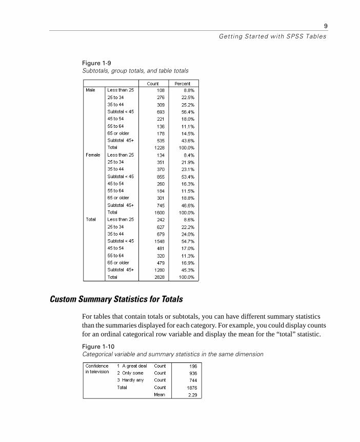
Totals and Subtotals
Tables provides a great deal of control over the display of totals and subtotals, including:
� Overall row and column totals
� Group totals for nested, stacked, and layered tables
� Subgroup totals
9
Getting Started with SPSS Tables
Figure 1-9Subtotals, group totals, and table totals
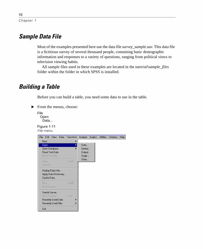
Custom Summary Statistics for Totals
For tables that contain totals or subtotals, you can have different summary statistics than the summaries displayed for each category. For example, you could display counts for an ordinal categorical row variable and display the mean for the “total” statistic.
Figure 1-10Categorical variable and summary statistics in the same dimension
10
Chapter 1
Sample Data File
Most of the examples presented here use the data file survey_sample.sav. This data file is a fictitious survey of several thousand people, containing basic demographic information and responses to a variety of questions, ranging from political views to television viewing habits.
All sample files used in these examples are located in the tutorial\sample_files folder within the folder in which SPSS is installed.
Building a Table
Before you can build a table, you need some data to use in the table.
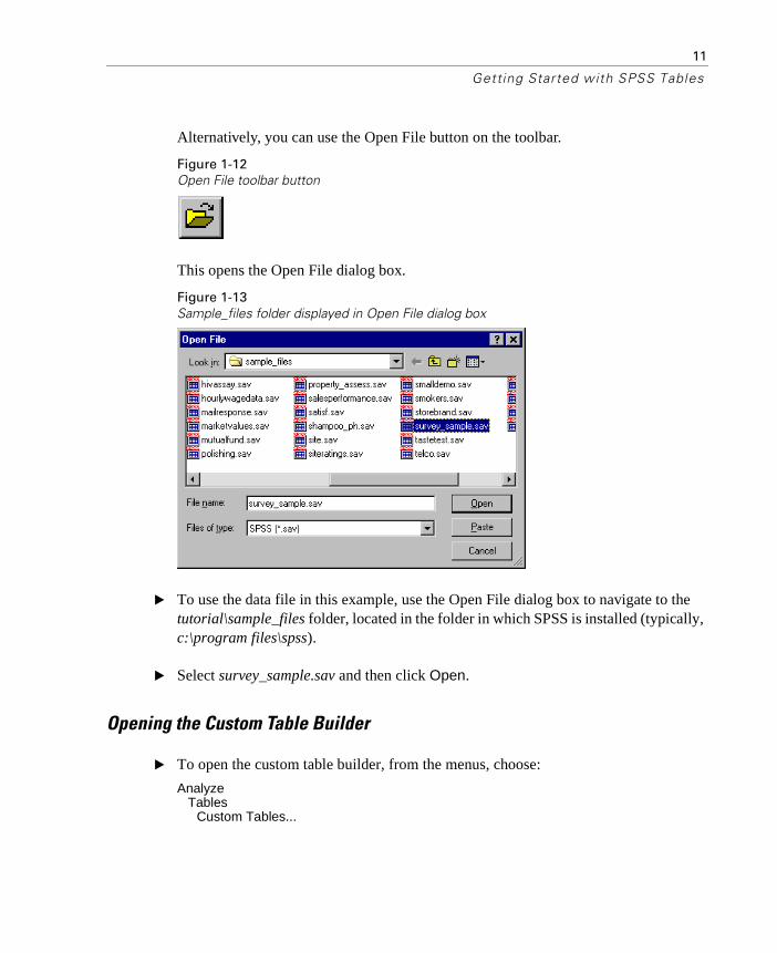
� From the menus, choose:
File Open
Data...
Figure 1-11File menu
11
Getting Started with SPSS Tables
Alternatively, you can use the Open File button on the toolbar.
Figure 1-12Open File toolbar button
This opens the Open File dialog box.
Figure 1-13Sample_files folder displayed in Open File dialog box
� To use the data file in this example, use the Open File dialog box to navigate to the tutorial\sample_files folder, located in the folder in which SPSS is installed (typically, c:\program files\spss).
� Select survey_sample.sav and then click Open.
Opening the Custom Table Builder
� To open the custom table builder, from the menus, choose:
Analyze Tables
Custom Tables...

12
Chapter 1
Figure 1-14Analyze menu, Tables
This opens the custom table builder.
Figure 1-15Custom table builder

13
Getting Started with SPSS Tables
Selecting Row and Column Variables
To create a table, you simply drag and drop variables where you want them to appear in the table.
� Select (click) Age category in the variable list and drag and drop it into the Rows area on the canvas pane.
Figure 1-16Selecting a row variable
The canvas pane displays the table that would be created using this single row variable. The preview does not display the actual values that would be displayed in the table;
it displays only the basic layout of the table.
� Select Gender in the variable list and drag and drop it into the Columns area on the canvas pane (you may have to scroll down the variable list to find this variable).
14
Chapter 1
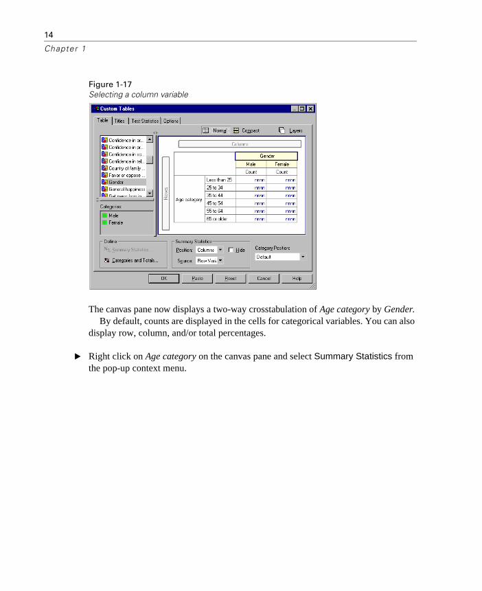
Figure 1-17Selecting a column variable
The canvas pane now displays a two-way crosstabulation of Age category by Gender. By default, counts are displayed in the cells for categorical variables. You can also
display row, column, and/or total percentages.
� Right click on Age category on the canvas pane and select Summary Statistics from the pop-up context menu.
15
Getting Started with SPSS Tables
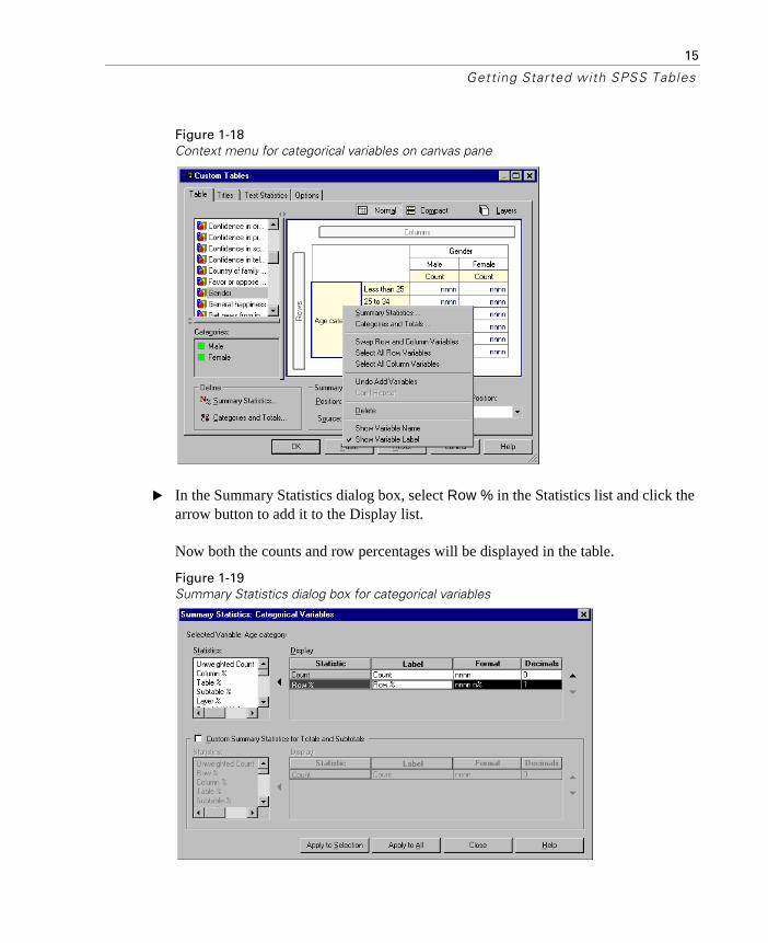
Figure 1-18Context menu for categorical variables on canvas pane
� In the Summary Statistics dialog box, select Row % in the Statistics list and click the arrow button to add it to the Display list.
Now both the counts and row percentages will be displayed in the table.
Figure 1-19Summary Statistics dialog box for categorical variables
16
Chapter 1
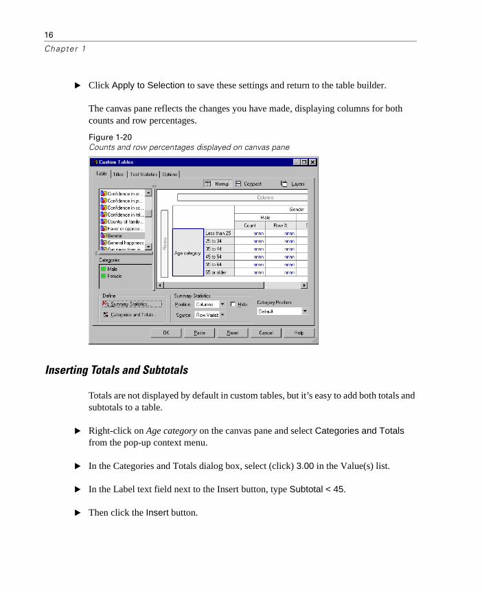
� Click Apply to Selection to save these settings and return to the table builder.
The canvas pane reflects the changes you have made, displaying columns for both counts and row percentages.
Figure 1-20Counts and row percentages displayed on canvas pane
Inserting Totals and Subtotals
Totals are not displayed by default in custom tables, but it’s easy to add both totals and subtotals to a table.
� Right-click on Age category on the canvas pane and select Categories and Totals from the pop-up context menu.
� In the Categories and Totals dialog box, select (click) 3.00 in the Value(s) list.
� In the Label text field next to the Insert button, type Subtotal < 45.
� Then click the Insert button.

17
Getting Started with SPSS Tables
This inserts a row containing the subtotal for the first three age categories.
� Select (click) 6.00 in the Value(s) list.
� In the Label text field next to the Insert button, type Subtotal 45+.
� Then click the Insert button.
This inserts a row containing the subtotal for the last three age categories.
� To include an overall total, select the Total check box.
Figure 1-21Inserting totals and subtotals
� Then click Apply.
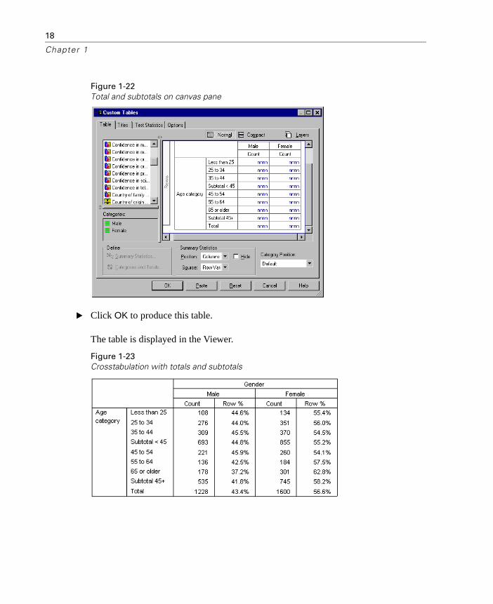
The canvas pane preview now includes rows for the two subtotals and the overall total.
18
Chapter 1
Figure 1-22Total and subtotals on canvas pane
� Click OK to produce this table.
The table is displayed in the Viewer.
Figure 1-23Crosstabulation with totals and subtotals
19
Getting Started with SPSS Tables
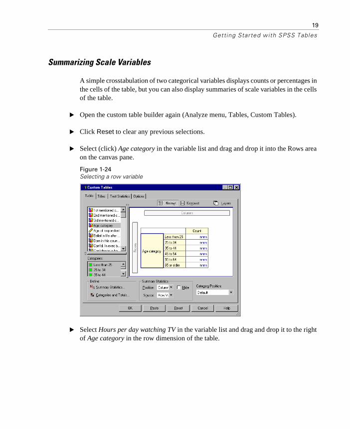
Summarizing Scale Variables
A simple crosstabulation of two categorical variables displays counts or percentages in the cells of the table, but you can also display summaries of scale variables in the cells of the table.
� Open the custom table builder again (Analyze menu, Tables, Custom Tables).
� Click Reset to clear any previous selections.
� Select (click) Age category in the variable list and drag and drop it into the Rows area on the canvas pane.
Figure 1-24Selecting a row variable
� Select Hours per day watching TV in the variable list and drag and drop it to the right of Age category in the row dimension of the table.
20
Chapter 1
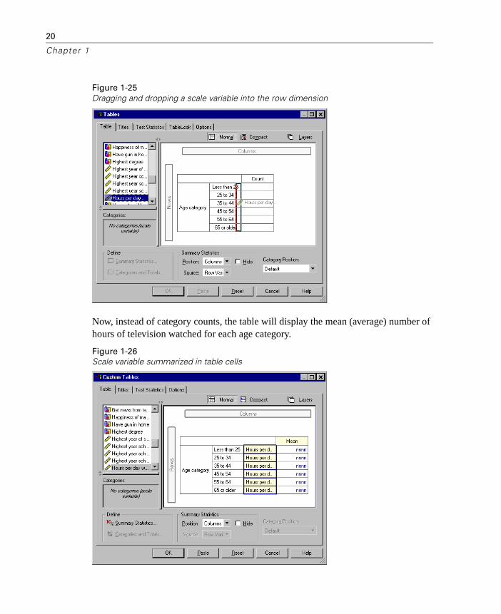
Figure 1-25Dragging and dropping a scale variable into the row dimension
Now, instead of category counts, the table will display the mean (average) number of hours of television watched for each age category.
Figure 1-26Scale variable summarized in table cells

21
Getting Started with SPSS Tables
The mean is the default summary statistic for scale variables. You can add or change the summary statistics displayed in the table.
� Right-click the scale variable on the canvas pane, and select Summary Statistics from the pop-up context menu.
Figure 1-27Context menu for scale variables in table preview
� In the Summary Statistics dialog box, select Median in the Statistics list and click the arrow button to add it to the Display list.
Now both the mean and the median will be displayed in the table.
Figure 1-28Summary Statistics dialog box for scale variables

22
Chapter 1
� Click Apply to Selection to save these settings and return to the table builder.
The canvas pane now shows that both the mean and median will be displayed in the table.
Figure 1-29Mean and median scale summaries displayed on canvas pane
Before creating this table, let’s clean it up a bit.
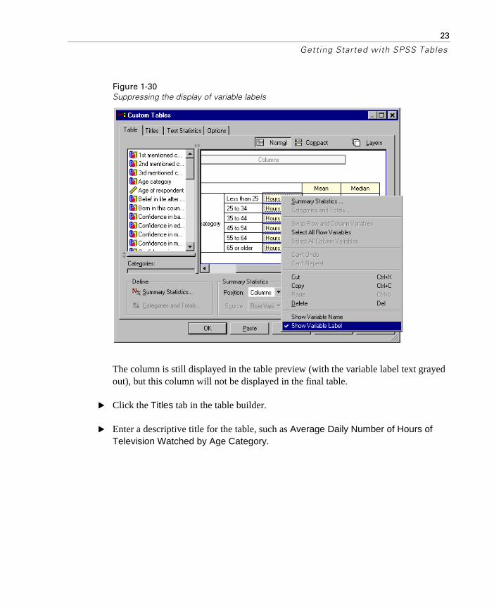
� Right-click on Hours per day... on the canvas pane and deselect (uncheck) Show Variable Label on the pop-up context menu.
23
Getting Started with SPSS Tables
Figure 1-30Suppressing the display of variable labels
The column is still displayed in the table preview (with the variable label text grayed out), but this column will not be displayed in the final table.
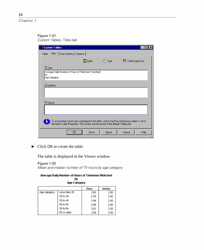
� Click the Titles tab in the table builder.
� Enter a descriptive title for the table, such as Average Daily Number of Hours of Television Watched by Age Category.
24
Chapter 1
Figure 1-31Custom Tables, Titles tab
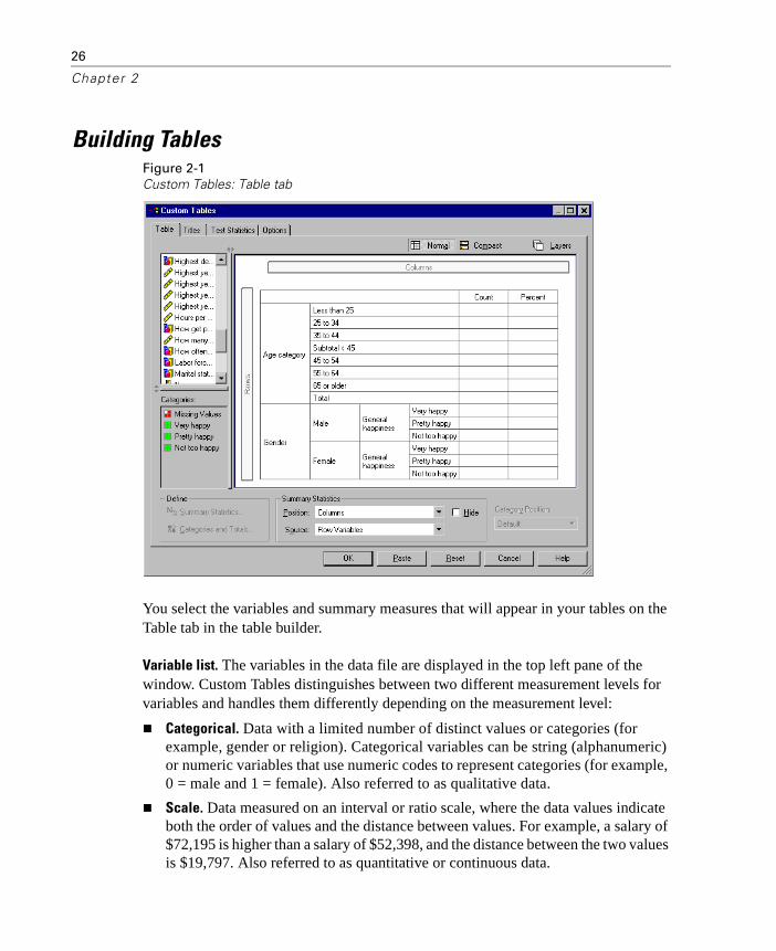
� Click OK to create the table.
The table is displayed in the Viewer window.
Figure 1-32Mean and median number of TV hours by age category

25
Chapte r
2Table Builder Interface
Custom Tables uses a simple drag-and-drop table builder interface that allows you to preview your table as you select variables and options. It also provides a level of flexibility not found in a typical “dialog box,” including the ability to change the size of the window and the size of the panes within the window.
26
Chapter 2
Building TablesFigure 2-1Custom Tables: Table tab
You select the variables and summary measures that will appear in your tables on the Table tab in the table builder.
Variable list. The variables in the data file are displayed in the top left pane of the window. Custom Tables distinguishes between two different measurement levels for variables and handles them differently depending on the measurement level:
� Categorical. Data with a limited number of distinct values or categories (for example, gender or religion). Categorical variables can be string (alphanumeric) or numeric variables that use numeric codes to represent categories (for example, 0 = male and 1 = female). Also referred to as qualitative data.
� Scale. Data measured on an interval or ratio scale, where the data values indicate both the order of values and the distance between values. For example, a salary of $72,195 is higher than a salary of $52,398, and the distance between the two values is $19,797. Also referred to as quantitative or continuous data.
27
Table Bui lder Interface
Categorical variables define categories (row, columns, and layers) in the table, and the default summary statistic is the count (number of cases in each category). For example, a default table of a categorical gender variable would simply display the number of males and the number of females.
Scale variables are typically summarized within categories of categorical variables, and the default summary statistic is the mean. For example, a default table of income within gender categories would display the mean income for males and the mean income for females.
You can also summarize scale variables by themselves, without using a categorical variable to define groups. This is primarily useful for stacking summaries of multiple scale variables. For more information, see “Stacking Variables” below.
Multiple Response Sets
Custom Tables also supports a special kind of “variable” called a multiple response set. Multiple response sets aren’t really “variables” in the normal sense. You can’t see them in the Data Editor, and other procedures don’t recognize them. Multiple response sets use multiple variables to record responses to questions where the respondent can give more than one answer. Multiple response sets are treated like categorical variables, and most of the things you can do with categorical variables, you can also do with multiple response sets. For more information, see the chapter Multiple Response Sets.
An icon next to each variable in the variable list identifies the variable type.
You can change the measurement level of a variable in the table builder by right-clicking the variable in the variable list and selecting Categorical or Scale from the pop-up context menu. You can permanently change a variable’s measurement level in
Scale
Categorical
Multiple response set, multiple categories
Multiple response set, multiple dichotomies
28
Chapter 2
the Variable View of the Data Editor. Variables defined as nominal or ordinal are treated as categorical by Custom Tables.
Categories. When you select a categorical variable in the variable list, the defined categories for the variable are displayed in the Categories list. These categories will also be displayed on the canvas pane when you use the variable in a table. If the variable has no defined categories, the Categories list and the canvas pane will display two placeholder categories: Category 1 and Category 2.
The defined categories displayed in the table builder are based on value labels, descriptive labels assigned to different data values (for example, numeric values of 0 and 1, with value labels of male and female). You can define value labels in Variable View of the Data Editor or with Define Variable Properties on the Data menu in the Data Editor window.
Canvas pane. You build a table by dragging and dropping variables onto the rows and columns of the canvas pane. The canvas pane displays a preview of the table that will be created. The canvas pane doesn’t show actual data values in the cells, but it should provide a fairly accurate view of the layout of the final table. For categorical variables, the actual table may contain more categories than the preview if the data file contains unique values for which no value labels have been defined.
� Normal view displays all of the rows and columns that will be included in the table, including rows and/or columns for summary statistics and categories of categorical variables.
� Compact view shows only the variables that will be in the table, without a preview of the rows and columns that the table will contain.
Basic Rules and Limitations for Building a Table
� For categorical variables, summary statistics are based on the innermost variable in the statistics source dimension.
� The default statistics source dimension (row or column) for categorical variables is based on the order in which you drag and drop variables into the canvas pane. For example, if you drag a variable to the rows tray first, the row dimension is the default statistics source dimension.
� Scale variables can be summarized only within categories of the innermost variable in either the row or column dimension. (You can position the scale variable at any level of the table, but it is summarized at the innermost level.)
29
Table Bui lder Interface
� Scale variables cannot be summarized within other scale variables. You can stack summaries of multiple scale variables or summarize scale variables within categories of categorical variables. You cannot nest one scale variable within another or put one scale variable in the row dimension and another scale variable in the column dimension.
To Build a Table
� From the menus, choose:
Analyze Tables
Custom Tables...
� Drag and drop one or more variables to the row and/or column areas of the canvas pane.
� Click OK to create the table.
To delete a variable from the canvas pane in the table builder:
� Select (click) the variable on the canvas pane.
� Drag the variable anywhere outside the canvas pane, or press the Delete key.
To change the measurement level of a variable:
� Right-click the variable in the variable list (you can do this only in the variable list, not on the canvas).
� Select Categorical or Scale from the pop-up context menu.
Stacking Variables
Stacking can be thought of as taking separate tables and pasting them together into the same display. For example, you could display information on gender and age category in separate sections of the same table.
30
Chapter 2
To Stack Variables
� In the variable list, select all of the variables you want to stack, and drag and drop them together into the rows or columns of the canvas pane.
or
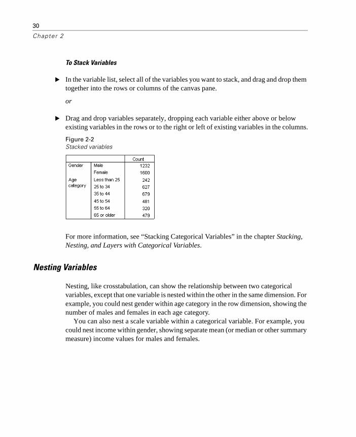
� Drag and drop variables separately, dropping each variable either above or below existing variables in the rows or to the right or left of existing variables in the columns.
Figure 2-2Stacked variables
For more information, see “Stacking Categorical Variables” in the chapter Stacking, Nesting, and Layers with Categorical Variables.
Nesting Variables
Nesting, like crosstabulation, can show the relationship between two categorical variables, except that one variable is nested within the other in the same dimension. For example, you could nest gender within age category in the row dimension, showing the number of males and females in each age category.
You can also nest a scale variable within a categorical variable. For example, you could nest income within gender, showing separate mean (or median or other summary measure) income values for males and females.
31
Table Bui lder Interface
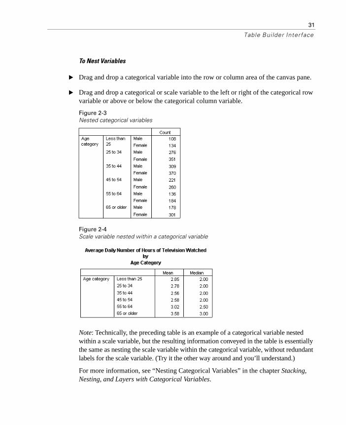
To Nest Variables
� Drag and drop a categorical variable into the row or column area of the canvas pane.
� Drag and drop a categorical or scale variable to the left or right of the categorical row variable or above or below the categorical column variable.
Figure 2-3Nested categorical variables
Figure 2-4Scale variable nested within a categorical variable
Note: Technically, the preceding table is an example of a categorical variable nested within a scale variable, but the resulting information conveyed in the table is essentially the same as nesting the scale variable within the categorical variable, without redundant labels for the scale variable. (Try it the other way around and you’ll understand.)
For more information, see “Nesting Categorical Variables” in the chapter Stacking, Nesting, and Layers with Categorical Variables.
32
Chapter 2
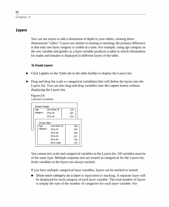
Layers
You can use layers to add a dimension of depth to your tables, creating three-dimensional “cubes.” Layers are similar to nesting or stacking; the primary difference is that only one layer category is visible at a time. For example, using age category as the row variable and gender as a layer variable produces a table in which information for males and females is displayed in different layers of the table.
To Create Layers
� Click Layers on the Table tab in the table builder to display the Layers list.
� Drag and drop the scale or categorical variable(s) that will define the layers into the Layers list. You can also drag and drop variables onto the Layers button without displaying the Layers list.
Figure 2-5Layered variables
You cannot mix scale and categorical variables in the Layers list. All variables must be of the same type. Multiple response sets are treated as categorical for the Layers list. Scale variables in the layers are always stacked.
If you have multiple categorical layer variables, layers can be stacked or nested.
� Show each category as a layer is equivalent to stacking. A separate layer will be displayed for each category of each layer variable. The total number of layers is simply the sum of the number of categories for each layer variable. For
33
Table Bui lder Interface
example, if you have three layer variables, each with three categories, the table will have nine layers.
� Show each combination of categories as a layer is equivalent to nesting or crosstabulating layers. The total number of layers is the product of the number of categories for each layer variable. For example, if you have three variables, each with three categories, the table will have 27 layers.
Showing and Hiding Variable Names and/or Labels
The following options are available for the display of variable names and labels:
� Show only variable labels. For any variables without defined variable labels, the variable name is displayed. This is the default setting.
� Show only variable names.
� Show both variable labels and variable names.
� Don’t show variable names or variable labels. Although the column/row that contains the variable label or name will still be displayed in the table preview on the canvas pane, this column/row will not be displayed in the actual table.
To show or hide variable labels or variable names:
� Right-click the variable in the table preview on the canvas pane.
� Select Show Variable Label or Show Variable Name from the pop-up context menu to toggle the display of labels or names on or off. A check mark next to the selection indicates that it will be displayed.
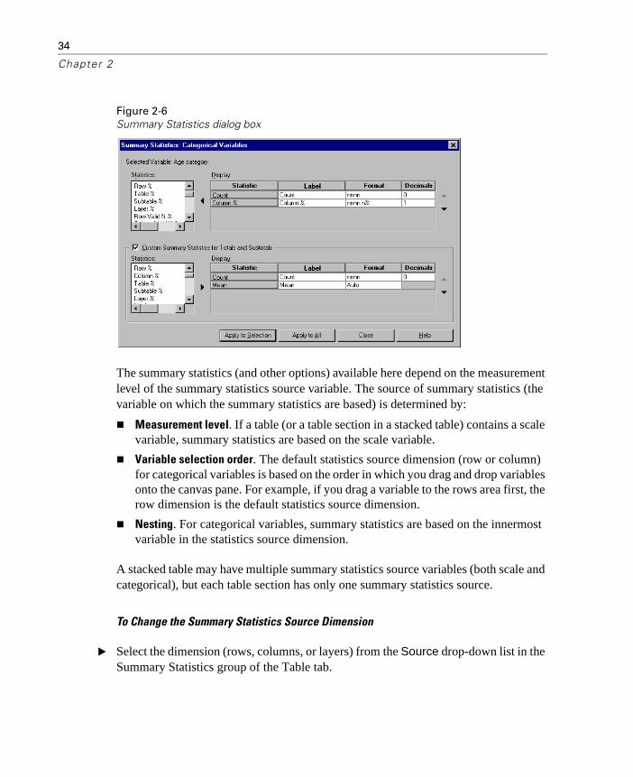
Summary Statistics
The Summary Statistics dialog box allows you to:
� Add and remove summary statistics from a table.
� Change the labels for the statistics.
� Change the order of the statistics.
� Change the format of the statistics, including the number of decimal positions.
34
Chapter 2
Figure 2-6Summary Statistics dialog box
The summary statistics (and other options) available here depend on the measurement level of the summary statistics source variable. The source of summary statistics (the variable on which the summary statistics are based) is determined by:
� Measurement level. If a table (or a table section in a stacked table) contains a scale variable, summary statistics are based on the scale variable.
� Variable selection order. The default statistics source dimension (row or column) for categorical variables is based on the order in which you drag and drop variables onto the canvas pane. For example, if you drag a variable to the rows area first, the row dimension is the default statistics source dimension.
� Nesting. For categorical variables, summary statistics are based on the innermost variable in the statistics source dimension.
A stacked table may have multiple summary statistics source variables (both scale and categorical), but each table section has only one summary statistics source.
To Change the Summary Statistics Source Dimension
� Select the dimension (rows, columns, or layers) from the Source drop-down list in the Summary Statistics group of the Table tab.

35
Table Bui lder Interface
To Control the Summary Statistics Displayed in a Table
� Select (click) the summary statistics source variable on the canvas pane of the Table tab.
� In the Define group of the Table tab, click Summary Statistics.
or
� Right-click the summary statistics source variable on the canvas pane and select Summary Statistics from the pop-up context menu.
� Select the summary statistics you want to include in the table. You can use the arrow to move selected statistics from the Statistics list to the the Display list, or you can drag and drop selected statistics from the Statistics list into the Display list.
� Click the up or down arrows to change the display position of the currently selected summary statistic.
� Select a display format from the Format drop-down list for the selected summary statistic.
� Enter the number of decimals to display in the Decimals cell for the selected summary statistic.
� Click Apply to Selection to include the selected summary statistics for the currently selected variables on the canvas pane.
� Click Apply to All to include the selected summary statistics for all stacked variables of the same type on the canvas pane.
Note: Apply to All differs from Apply to Selection only for stacked variables of the same type already on the canvas pane. In both cases, the selected summary statistics are automatically included for any additional stacked variables of the same type that you add to the table.

36
Chapter 2
Summary Statistics for Categorical Variables
The basic statistics available for categorical variables are counts and percentages. You can also specify custom summary statistics for totals and subtotals. These custom summary statistics include measures of central tendency (such as mean and median) and dispersion (such as standard deviation) that may be suitable for some ordinal categorical variables. For more information, see “Custom Total Summary Statistics for Categorical Variables” below.
Count. Number of cases in each cell of the table or number of responses for multiple response sets.
Unweighted Count. Unweighted number of cases in each cell of the table.
Column percentages. Percentages within each column. The percentages in each column of a subtable (for simple percentages) sum to 100%. Column percentages are typically useful only if you have a categorical row variable.
Row percentages. Percentages within each row. The percentages in each row of a subtable (for simple percentages) sum to 100%. Row percentages are typically useful only if you have a categorical column variable.
Layer Row and Layer Column percentages. Row or column percentages (for simple percentages) sum to 100% across all subtables in a nested table. If the table contains layers, row or column percentages sum to 100% across all nested subtables in each layer.
Layer percentages. Percentages within each layer. For simple percentages, cell percentages within the currently visible layer sum to 100%. If you don’t have any layer variables, this is equivalent to table percentages.
Table percentages. Percentages for each cell are based on the entire table. All cell percentages are based on the same total number of cases and sum to 100% (for simple percentages) over the entire table.
Subtable percentages. Percentages in each cell are based on the subtable. All cell percentages in the subtable are based the same total number of cases and sum to 100% within the subtable. In nested tables, the variable that precedes the innermost nesting level defines subtables. For example, in a table of marital status within gender within age category, gender defines subtables.
Multiple response sets can have percentages based on cases, responses, or counts. For more information, see “Summary Statistics for Multiple Response Sets” below.

37
Table Bui lder Interface
Stacked Tables
For percentage calculations, each table section defined by a stacking variable is treated as a separate table. Layer Row, Layer Column, and Table percentages sum to 100% (for simple percentages) within each stacked table section. The percentage base for different percentage calculations is based on the cases in each stacked table section.
Percentage Base
Percentages can be calculated in three different ways, determined by the treatment of missing values in the base (denominator):
Simple percentage. Percentatges are based on the number of cases used in the table and always sum to 100%. If a category is excluded from the table, cases in that category are excluded from the base. Cases with system-missing values are always excluded from the base. Cases with user-missing values are excluded if user-missing categories are excluded from the table (the default) or included if user-missing categories are included in the table. Any percentage that doesn’t have “Valid N” or “Total N” in its name is a simple percentage.
Total N percentage. Cases with system-missing and user-missing values are added to the Simple percentage base. Percentages may sum to less than 100%.
Valid N percentage. Cases with user-missing values are removed from the Simple percentage base even if user-missing categories are included in the table. Percentages may sum to more than 100%.
Note: Cases in manually excluded categories other than user-missing categories are always excluded from the base.
Summary Statistics for Multiple Response Sets
The following additional summary statistics are available for multiple response sets.
Col/Row/Layer Responses %. Percentage based on responses.
Col/Row/Layer Responses % (Base: Count). Responses are the numerator and total count is the denominator.
Col/Row/Layer Count % (Base: Responses). Count is the numerator and total responses are the denominator.
38
Chapter 2
Layer Col/Row Responses %. Percentage across subtables. Percentage based on responses.
Layer Col/Row Responses % (Base: Count). Percentages across subtables. Responses are the numerator and total count is the denominator.
Layer Col/RowResponses % (Base: Responses). Percentages across subtables. Count is the numerator and total responses is the denominator.
Responses. Count of responses.
Subtable/Table Responses %. Percentage based on responses.
Subtable/Table Responses % (Base: Count). Responses are the numerator and total count is the denominator.
Subtable/Table Count % (Base: Responses). Count is the numerator and total responses are the denominator.
Summary Statistics for Scale Variables and Categorical Custom Totals
In addition to the counts and percentages available for categorical variables, the following summary statistics are available for scale variables and as custom total and subtotal summaries for categorical variables. These summary statistics are not available for multiple response sets or string (alphanumeric) variables.
Mean. Arithmetic average; the sum divided by the number of cases.
Median. Value above and below which half of the cases fall; the 50th percentile.
Mode. Most frequent value. If there is a tie, the smallest value is shown.
Minimum. Smallest (lowest) value.
Maximum. Largest (highest) value.
Missing. Count of missing values (both user- and system-missing).
Percentile. You can include the 5th, 25th, 75th, 95th, and/or 99th percentiles.
Range. Difference between maximum and minimum values.
Standard error of the mean. A measure of how much the value of the mean may vary from sample to sample taken from the same distribution. It can be used to roughly compare the observed mean to a hypothesized value (that is, you can conclude that the
39
Table Bui lder Interface
two values are different if the ratio of the difference to the standard error is less than –2 or greater than +2).
Standard deviation. A measure of dispersion around the mean. In a normal distribution, 68% of the cases fall within one standard deviation of the mean and 95% of the cases fall within two standard deviations. For example, if the mean age is 45, with a standard deviation of 10, 95% of the cases would be between 25 and 65 in a normal distribution (the square root of the variance).
Sum. Sum of the values.
Sum percentage. Percentages based on sums. Available for rows and columns (within subtables), entire rows and columns (across subtables), layers, subtables, and entire tables.
Total N. Count of non-missing, user-missing, and system-missing values. Does not include cases in manually excluded categories other than user-missing categories.
Valid N. Count of non-missing values. Does not include cases in manually excluded categories other than user-missing categories.
Variance. A measure of dispersion around the mean, equal to the sum of squared deviations from the mean divided by one less than the number of cases. The variance is measured in units that are the square of those of the variable itself (the square of the standard deviation).
Stacked Tables
Each table section defined by a stacking variable is treated as a separate table, and summary statistics are calculated accordingly.
Custom Total Summary Statistics for Categorical Variables
For tables of categorical variables that contain totals or subtotals, you can have different summary statistics than the summaries displayed for each category. For example, you could display counts and column percentages for an ordinal categorical row variable and display the median for the “total” statistic.
40
Chapter 2
To create a table for a categorical variable with a custom total summary statistic:
� Open the table builder (Analyze menu, Tables, Custom Tables).
� Drag and drop a categorical variable into the Rows or Columns area of the canvas.
� Right-click on the variable on the canvas and select Categories and Totals from the pop-up context menu.
� Click (check) the Total check box, and then click Apply.
� Right-click the variable again on the canvas and select Summary Statistics from the pop-up context menu.
� Click (check) Custom Summary Statistics for Totals and Subtotals, and then select the custom summary statistics you want.
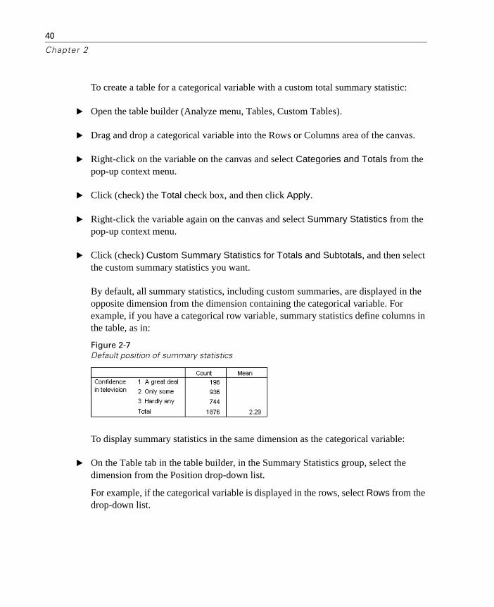
By default, all summary statistics, including custom summaries, are displayed in the opposite dimension from the dimension containing the categorical variable. For example, if you have a categorical row variable, summary statistics define columns in the table, as in:
Figure 2-7Default position of summary statistics
To display summary statistics in the same dimension as the categorical variable:
� On the Table tab in the table builder, in the Summary Statistics group, select the dimension from the Position drop-down list.
For example, if the categorical variable is displayed in the rows, select Rows from the drop-down list.

41
Table Bui lder Interface
Figure 2-8Categorical variable and summary statistics in the same dimension
Summary Statistics Display Formats
The following display format options are available:
nnnn. Simple numeric.
nnnn%. Percent sign appended to end of value.
Auto. Defined variable display format, including number of decimals.
N=nnnn. Displays "N=" before the value. This can be useful for counts, valid N, and total N in tables where the summary statistics labels are not displayed.
(nnnn). All values enclosed in parentheses.
(nnnn)(neg. value). Only negative values enclosed in parentheses.
(nnnn%). All values enclosed in parentheses and percent sign appended to end of values.
n,nnn.n. Comma format. Comma used as grouping separator and period used as decimal indicator regardless of locale settings.
n.nnn,n. Dot format. Period used as grouping separator and comma used as decimal indicator regardless of locale settings.
$n,nnn.n. Dollar format. Dollar sign displayed in front of value; comma used as grouping separator and period used as decimal indicator regardless of locale settings.
CCA, CCB, CCC, CCD, CCE. Custom currency formats. The current defined format for each custom currency is displayed in the list. These formats are defined on the Currency tab in the SPSS Options dialog box (Edit menu, Options).

42
Chapter 2
General Rules and Limitations
� With the exception of Auto, the number of decimals is determined by the Decimals column setting.
� With the exception of the comma, dollar, and dot formats, the decimal indicator used is the one defined for the current locale in your Windows Regional Options control panel.
� Although comma/dollar and dot will display either a comma or period respectively as the grouping separator, there is no display format available at creation time to display a grouping separator based on the current locale settings (defined in the Windows Regional Options control panel).
Categories and Totals
The Categories and Totals dialog box allows you to:
� Reorder and exclude categories.
� Insert subtotals and totals.
� Include or exclude empty categories.
� Include or exclude categories defined as containing missing values.
� Include or exclude categories that do not have defined value labels.

43
Table Bui lder Interface
Figure 2-9Categories and Totals dialog box
� This dialog box is available only for categorical variables and multiple response sets. It is not available for scale variables.
� For multiple selected variables with different categories, you cannot insert subtotals, exclude categories, or manually reorder categories. This occurs only if you select multiple variables in the canvas preview and access this dialog box for all selected variables simultaneously. You can still perform these actions for each variable separately.
� For variables with no defined value labels, you can only sort categories and insert totals.

44
Chapter 2
To Access the Categories and Totals Dialog Box
� Drag and drop a categorical variable or multiple response set onto the canvas pane.
� Right-click the variable on the canvas pane, and select Categories and Totals from the pop-up context menu.
or
� Select (click) the variable on the canvas pane, and then click Categories and Totals in the Define group on the Table tab.
You can also select multiple categorical variables in the same dimension on the canvas pane:
� Ctrl-click each variable on the canvas pane.
or
� Click outside the table preview on the canvas pane, and then click and drag to select the area that includes the variables you want to select.
or
� Right-click any variable in a dimension and select Select All [dimension] Variables to select all of the variables in that dimension.
To Reorder Categories
To manually reorder categories:
� Select (click) a category in the list.
� Click the up or down arrow to move the category up or down in the list.
or
� Click in the Value(s) column for the category, and drag and drop it in a different position.
45
Table Bui lder Interface
To Exclude Categories
� Select (click) a category in the list.
� Click the arrow next to the Exclude list.
or
� Click in the Value(s) column for the category and drag and drop it anywhere outside the list.
If you exclude any categories, any categories without defined value labels will also be excluded.
To Sort Categories
You can sort categories by data value, value label, or cell count in ascending or descending order.
� In the Sort Categories group, click the By drop-down list and select the sort criterion you want to use (value, label, or cell count).
� Click the Order drop-down list to select the sort order (ascending or descending).
Sorting categories is not available if you have excluded any categories.
Subtotals
� Select (click) the category in the list that is the last category in the range of categories that you want to include in the subtotal.
� Click Insert. You can also modify the subtotal label text.
Totals
� Click the Total check box. You can also modify the total label text.
If the selected variable is nested within another variable, totals will be inserted for each subtable.

46
Chapter 2
Display Position for Totals and Subtotals
Totals and subtotals can be displayed above or below the categories included in each total.
� If Below is selected in the Totals and Subtotals Appear group, totals appear above each subtable, and all categories above and including the selected category (but below any preceding subtotals) are included in each subtotal.
� If Above is selected in the Totals and Subtotals Appear group, totals appear below each subtable, and all categories below and including the selected category (but above any preceding subtotals) are included in each subtotal.
Important: You should select the display position for subtotals before defining any subtotals. Changing the display position affects all subtotals (not just the currently selected subtotal), and it also changes the categories included in the subtotals.
Custom Total and Subtotal Summary Statistics
You can display statistics other than “totals” in the Totals and Subtotals areas of the table using the Summary Statistics dialog box. For more information, see “Summary Statistics for Categorical Variables” above.
Totals, Subtotals, and Excluded Categories
Cases from excluded categories are not included in the calculation of totals.
Missing Values, Empty Categories, and Values without Value Labels
Missing values. This controls the display of user-missing values, or values defined as containing missing values (for example, a code of 99 to represent “not applicable” for pregnancy in males). By default, user-missing values are excluded. Select (check) this option to include user-missing categories in tables. Although the variable may contain more than one missing value category, the table preview on the canvas will display only one generic missing value category. All defined user-missing categories will be included in the table. System-missing values (empty cells for numeric variables in the Data Editor) are always excluded.
47
Table Bui lder Interface
Empty categories. Empty categories are categories with defined value labels but no cases in that category for a particular table or subtable. By default, empty categories are included in tables. Deselect (uncheck) this option to exclude missing categories from the table.
Other values found when data are scanned. By default, category values in the data file that do not have defined value labels are automatically included in tables. Deselect (uncheck) this option to exclude values without defined value labels from the table. If you exclude any categories with defined value labels, categories without defined value labels are also excluded.
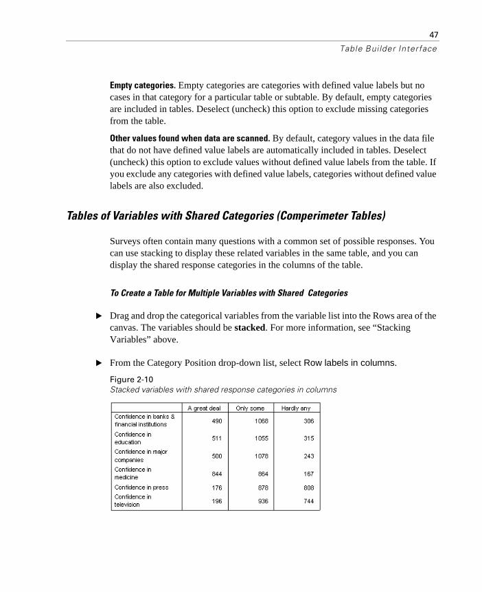
Tables of Variables with Shared Categories (Comperimeter Tables)
Surveys often contain many questions with a common set of possible responses. You can use stacking to display these related variables in the same table, and you can display the shared response categories in the columns of the table.
To Create a Table for Multiple Variables with Shared Categories
� Drag and drop the categorical variables from the variable list into the Rows area of the canvas. The variables should be stacked. For more information, see “Stacking Variables” above.
� From the Category Position drop-down list, select Row labels in columns.
Figure 2-10Stacked variables with shared response categories in columns

48
Chapter 2
Customizing the Table Builder
Unlike standard dialog boxes, you can change the size of the table builder in the same way that you can change the size of any standard window:
� Click and drag the top, bottom, either side, or any corner of the table builder to decrease or increase its size.
On the Table tab, you can also change the size of the variable list, the Categories list, and the canvas pane.
� Click and drag the horizontal bar between the variable list and the Categories list to make the lists longer or shorter. Moving it down makes the variable list longer and the Categories list shorter. Moving it up does the reverse.
� Click and drag the vertical bar between the variable list and Categories list from the canvas pane to make the lists wider or narrower. The canvas automatically resizes to fit the remaining space.
Custom Tables: Options Tab
The Options tab allows you to:
� Specify what is displayed in empty cells and cells for which statistics cannot be computed.
� Control how missing values are handled in the computation of scale variable statistics.
� Set minimum and/or maximum data column widths.
� Control the treatment of duplicate responses in multiple category sets.

49
Table Bui lder Interface
Figure 2-11Custom Tables: Options tab
Data Cell Appearance. Controls what is displayed in empty cells and cells for which statistics cannot be computed.
� Empty cells. For table cells that contain no cases (cell count of 0), you can select one of three display options: zero, blank, or a text value that you specify. The text value can be up to 255 characters long.
� Statistics that Cannot be Computed. Text displayed if a statistic cannot be computed (for example, the mean for a category with no cases). The text value can be up to 255 characters long. The default value is a period (.).
50
Chapter 2
Width for Data Columns. Controls minimum and maximum column width for data columns. This setting does not affect columns widths for row labels.
� TableLook settings. Uses the data column width specification from the current default TableLook. You can create your own custom default TableLook to use when new tables are created, and you can control both row label column and data column widths with a TableLook.
� Custom. Overrides the default TableLook settings for data column width. Specify the minimum and maximum data column widths for the table and the measurement unit: points, inches, or centimeters.
Missing Values for Scale Variables. For tables with two or more scale variables, controls the handling of missing data for scale variable statistics.
� Maximize use of available data (variable-by-variable deletion). All cases with valid values for each scale variable are included in summary statistics for that scale variable.
� Use consistent case base across scale variables (listwise deletion). Cases with missing values for any scale variables in the table are excluded from the summary statistics for all scale variables in the table.
Count duplicate responses for multiple category sets. A duplicate response is the same response for two or more variables in the multiple category set. By default, duplicate responses are not counted, but this may be a perfectly valid condition that you do want to include in the count (such as a multiple category set representing the manufacturer of the last three cars purchased by a survey respondent).
51
Table Bui lder Interface
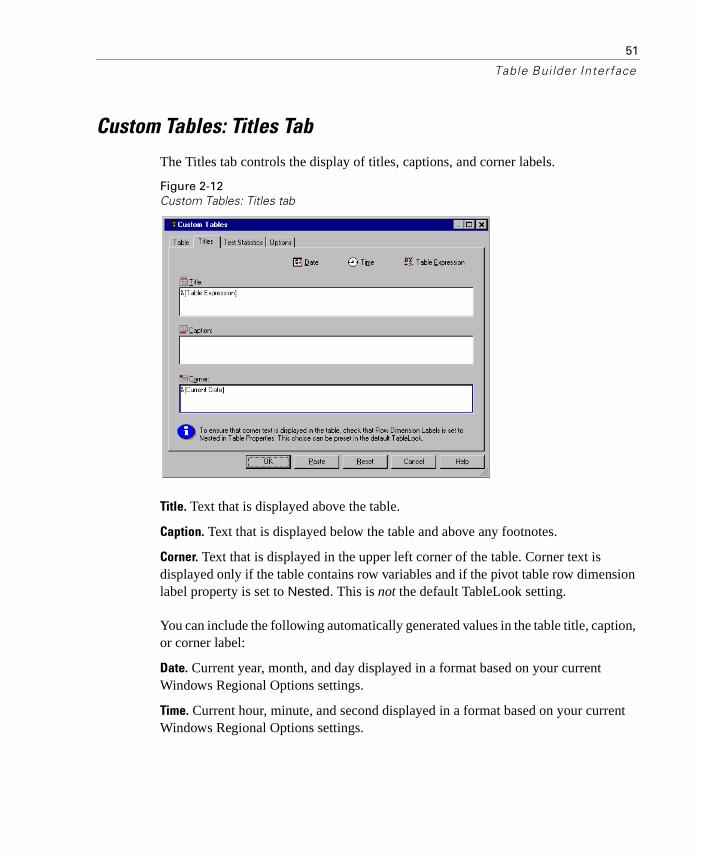
Custom Tables: Titles Tab
The Titles tab controls the display of titles, captions, and corner labels.
Figure 2-12Custom Tables: Titles tab
Title. Text that is displayed above the table.
Caption. Text that is displayed below the table and above any footnotes.
Corner. Text that is displayed in the upper left corner of the table. Corner text is displayed only if the table contains row variables and if the pivot table row dimension label property is set to Nested. This is not the default TableLook setting.
You can include the following automatically generated values in the table title, caption, or corner label:
Date. Current year, month, and day displayed in a format based on your current Windows Regional Options settings.
Time. Current hour, minute, and second displayed in a format based on your current Windows Regional Options settings.
52
Chapter 2
Table Expression. Variables used in the table and how they’re used in the table. If a variable has a defined variable label, the label is displayed. In the generated table, the following symbols indicate how variables are used in the table:
� + indicates stacked variables.
� > indicates nesting.
� BY indicates crosstabulation or layers.
Custom Tables: Test Statistics Tab
The Test Statistics tab allows you to request various significance tests for your custom tables, including:
� Chi-square tests of independence.
� Tests of the equality of column means.
� Tests of the equality of column proportions.
These tests are not available for multiple response variables or tables in which category labels are moved out of their default table dimension.

53
Table Bui lder Interface
Figure 2-13Custom Tables: Test Statistics tab
Tests of independence (Chi-square). This option produces a chi-square test of independence for tables in which at least one category variable exists in both the rows and columns. You can also specify the alpha level of the test, which should be a value greater than 0 and less than 1.
Compare column means (t-tests). This option produces pairwise tests of the equality of column means for tables in which at least one category variable exists in the columns and at least one scale variable exists in the rows. You can select whether the p values of the tests are adjusted using the Bonferroni method. You can also specify the alpha level of the test, which should be a value greater than 0 and less than 1.
Compare column proportions (z-tests). This option produces pairwise tests of the equality of column proportions for tables in which at least one category variable exists in both the columns and rows. You can select whether the p values of the tests are adjusted using the Bonferroni method. You can also specify the alpha level of the test, which should be a value greater than 0 and less than 1.

55
Chapte r
3Simple Tables for Categorical Variables
Most tables you want to create will probably include at least one categorical variable. A categorical variable is one with a limited number of distinct values or categories (for example, gender or religion).
An icon next to each variable in the variable list identifies the variable type.
Custom Tables is optimized for use with categorical variables that have defined value labels. For more information, see “Building Tables” in the chapter Table Builder Interface.
Sample Data File
The examples in this chapter use the data file survey_sample.sav. This file is located in the tutorial\sample_files folder within the folder in which SPSS is installed.
All examples provided here display variable labels in dialog boxes, sorted in alphabetical order. Variable list display properties are set on the General tab in the Options dialog box (Edit menu, Options).
Scale
Categorical
Multiple response set, multiple categories
Multiple response set, multiple dichotomies

56
Chapter 3
A Single Categorical Variable
Although a table of a single categorical variable may be one of the simplest tables you can create, it may often be all you want or need.
� From the menus, choose:
Analyze Tables
Custom Tables...
� In the table builder, drag and drop Age category from the variable list to the Rows area on the canvas pane.
A preview of the table is displayed on the canvas pane. The preview doesn’t display actual data values; it displays only placeholders where data will be displayed.
Figure 3-1A single categorical variable in rows

57
Simple Tables for Categorical Variables
� Click OK to create the table.
The table is displayed in the Viewer window.
Figure 3-2A single categorical variable in rows
In this simple table, the column heading Count isn’t really necessary, and you can create the table without this column heading.
� Open the table builder again (Analyze menu, Tables, Custom Tables).
� Select (click) Hide for Position in the Summary Statistics group.
� Click OK to create the table.
Figure 3-3Single categorical variable without summary statistics column label
Percentages
In addition to counts, you can also display percentages. For a simple table of a single categorical variable, if the variable is displayed in rows, you probably want to look at column percentages. Conversely, for a variable displayed in columns, you probably want to look at row percentages.

58
Chapter 3
� Open the table builder again (Analyze menu, Tables, Custom Tables).
� Deselect (uncheck) Hide for Position in the Summary Statistics group. Since this table will have two columns, you want to display the column labels so you know what each column represents.
� Right-click on Age category on the canvas pane and select Summary Statistics from the pop-up context menu.
Figure 3-4Right-click context menu on canvas pane
� In the Summary Statistics dialog box, select Column % in the Statistics list and click the arrow to add it to the Display list.
� In the Label cell in the Display list, delete the default label and type Percent.

59
Simple Tables for Categorical Variables
Figure 3-5Summary Statistics Categorical Variables dialog box
� Click Apply to Selection and then click OK in the table builder to create the table.
Figure 3-6Counts and column percentages
Totals
Totals are not automatically included in custom tables, but it’s easy to add totals to a table.
� Open the table builder again (Analyze menu, Tables, Custom Tables).
� Right-click on Age category on the canvas pane and select Categories and Totals from the pop-up context menu.
60
Chapter 3
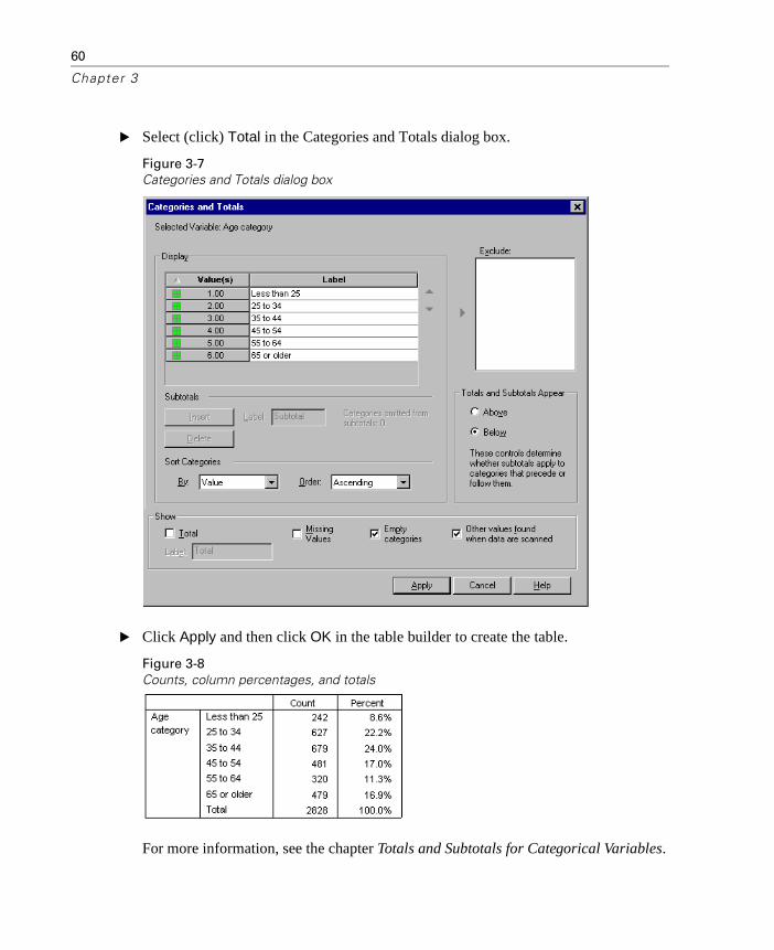
� Select (click) Total in the Categories and Totals dialog box.
Figure 3-7Categories and Totals dialog box
� Click Apply and then click OK in the table builder to create the table.
Figure 3-8Counts, column percentages, and totals
For more information, see the chapter Totals and Subtotals for Categorical Variables.
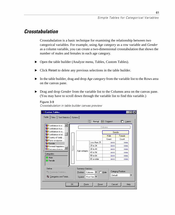
61
Simple Tables for Categorical Variables
Crosstabulation
Crosstabulation is a basic technique for examining the relationship between two categorical variables. For example, using Age category as a row variable and Gender as a column variable, you can create a two-dimensional crosstabulation that shows the number of males and females in each age category.
� Open the table builder (Analyze menu, Tables, Custom Tables).
� Click Reset to delete any previous selections in the table builder.
� In the table builder, drag and drop Age category from the variable list to the Rows area on the canvas pane.
� Drag and drop Gender from the variable list to the Columns area on the canvas pane. (You may have to scroll down through the variable list to find this variable.)
Figure 3-9Crosstabulation in table builder canvas preview
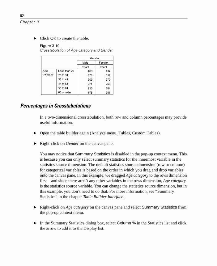
62
Chapter 3
� Click OK to create the table.
Figure 3-10Crosstabulation of Age category and Gender
Percentages in Crosstabulations
In a two-dimensional crosstabulation, both row and column percentages may provide useful information.
� Open the table builder again (Analyze menu, Tables, Custom Tables).
� Right-click on Gender on the canvas pane.
You may notice that Summary Statistics is disabled in the pop-up context menu. This is because you can only select summary statistics for the innermost variable in the statistics source dimension. The default statistics source dimension (row or column) for categorical variables is based on the order in which you drag and drop variables onto the canvas pane. In this example, we dragged Age category to the rows dimension first—and since there aren’t any other variables in the rows dimension, Age category is the statistics source variable. You can change the statistics source dimension, but in this example, you don’t need to do that. For more information, see “Summary Statistics” in the chapter Table Builder Interface.
� Right-click on Age category on the canvas pane and select Summary Statistics from the pop-up context menu.
� In the Summary Statistics dialog box, select Column % in the Statistics list and click the arrow to add it to the Display list.
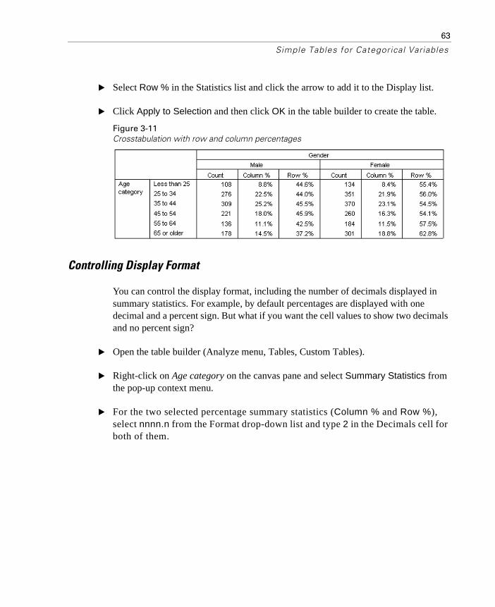
63
Simple Tables for Categorical Variables
� Select Row % in the Statistics list and click the arrow to add it to the Display list.
� Click Apply to Selection and then click OK in the table builder to create the table.
Figure 3-11Crosstabulation with row and column percentages
Controlling Display Format
You can control the display format, including the number of decimals displayed in summary statistics. For example, by default percentages are displayed with one decimal and a percent sign. But what if you want the cell values to show two decimals and no percent sign?
� Open the table builder (Analyze menu, Tables, Custom Tables).
� Right-click on Age category on the canvas pane and select Summary Statistics from the pop-up context menu.
� For the two selected percentage summary statistics (Column % and Row %), select nnnn.n from the Format drop-down list and type 2 in the Decimals cell for both of them.
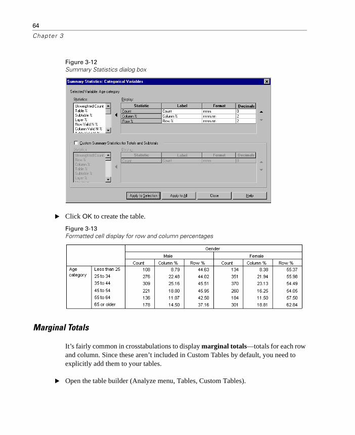
64
Chapter 3
Figure 3-12Summary Statistics dialog box
� Click OK to create the table.
Figure 3-13Formatted cell display for row and column percentages
Marginal Totals
It’s fairly common in crosstabulations to display marginal totals—totals for each row and column. Since these aren’t included in Custom Tables by default, you need to explicitly add them to your tables.
� Open the table builder (Analyze menu, Tables, Custom Tables).

65
Simple Tables for Categorical Variables
� Click Reset to delete any previous selections in the table builder.
� In the table builder, drag and drop Age category from the variable list to the Rows area on the canvas pane.
� Drag and drop Gender from the variable list to the Columns area on the canvas pane. (You may have to scroll down through the variable list to find this variable.)
� Right-click on Age category on the canvas pane and select Categories and Totals from the pop-up context menu.
� Select (click) Total in the Categories and Totals dialog box and then click Apply.
� Right-click on Gender on the canvas pane and select Categories and Totals from the pop-up context menu.
� Select (click) Total in the Categories and Totals dialog box and then click Apply.
� Select (click) Hide for Position in the Summary Statistics group. (Since you’re displaying only counts, you don’t need to identify the “statistic” displayed in the data cells of the table.)
� Click OK to create the table.
Figure 3-14Crosstabulation with marginal totals
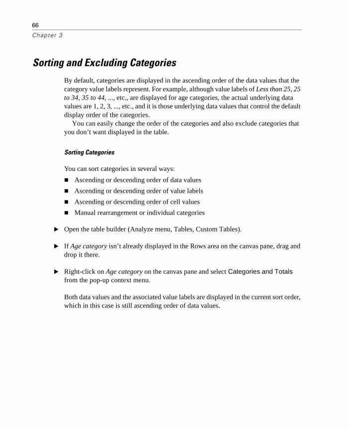
66
Chapter 3
Sorting and Excluding Categories
By default, categories are displayed in the ascending order of the data values that the category value labels represent. For example, although value labels of Less than 25, 25 to 34, 35 to 44, ..., etc., are displayed for age categories, the actual underlying data values are 1, 2, 3, ..., etc., and it is those underlying data values that control the default display order of the categories.
You can easily change the order of the categories and also exclude categories that you don’t want displayed in the table.
Sorting Categories
You can sort categories in several ways:
� Ascending or descending order of data values
� Ascending or descending order of value labels
� Ascending or descending order of cell values
� Manual rearrangement or individual categories
� Open the table builder (Analyze menu, Tables, Custom Tables).
� If Age category isn’t already displayed in the Rows area on the canvas pane, drag and drop it there.
� Right-click on Age category on the canvas pane and select Categories and Totals from the pop-up context menu.
Both data values and the associated value labels are displayed in the current sort order, which in this case is still ascending order of data values.

67
Simple Tables for Categorical Variables
Figure 3-15Default category order, ascending by data values
� In the Sort Categories group, select Descending from the Order drop-down list.
The sort order is now reversed.
� Select Labels from the By drop-down list.
The categories are now sorted in descending alphabetical order of the value labels.

68
Chapter 3
Figure 3-16Descending alphabetical sort order
Notice that the category labeled Less than 25 is at the top of the list. In alphabetical sorting, letters come after numbers. Since this is the only label that starts with a letter and since the list is sorted in descending (reverse) order, this category sorts to the top of the list.
If you want a particular category to appear at a different location in the list, you can easily move it.
� Click the category labeled Less than 25 in the Label list.
� Click the down arrow to the right of the list. The category moves down one row in the list.
� Keep clicking the down arrow until the category is at the bottom of the list.
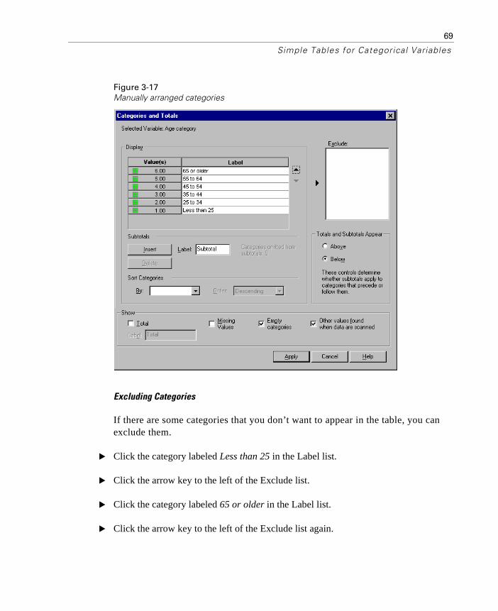
69
Simple Tables for Categorical Variables
Figure 3-17Manually arranged categories
Excluding Categories
If there are some categories that you don’t want to appear in the table, you can exclude them.
� Click the category labeled Less than 25 in the Label list.
� Click the arrow key to the left of the Exclude list.
� Click the category labeled 65 or older in the Label list.
� Click the arrow key to the left of the Exclude list again.

70
Chapter 3
The two categories are moved from the Display list to the Exclude list. If you change your mind, you can easily move them back to the Display list.
Figure 3-18Manually excluded categories in Categories and Totals dialog box
� Click Apply and then click OK in the table builder to create the table.
Figure 3-19Table sorted by descending value label, some categories excluded

71
Simple Tables for Categorical Variables
Notice that the totals are lower than they were before the two categories were excluded. This is because totals are based on the categories included in the table. Any excluded categories are excluded from the total calculation. For more information, see the chapter Totals and Subtotals for Categorical Variables.

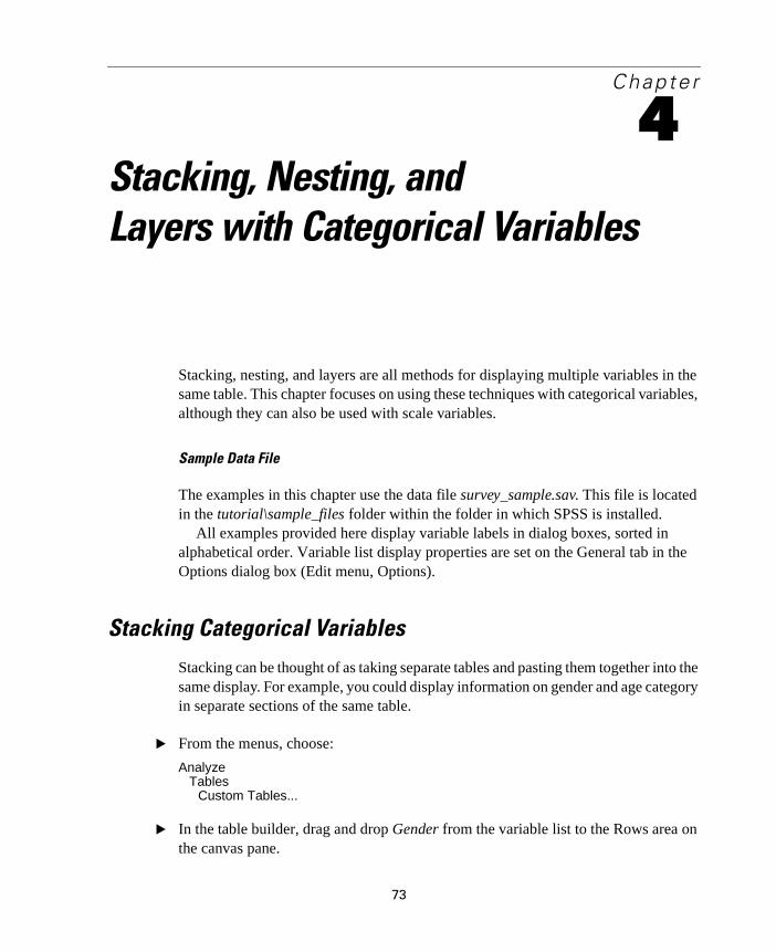
73
Chapte r
4Stacking, Nesting, and Layers with Categorical Variables
Stacking, nesting, and layers are all methods for displaying multiple variables in the same table. This chapter focuses on using these techniques with categorical variables, although they can also be used with scale variables.
Sample Data File
The examples in this chapter use the data file survey_sample.sav. This file is located in the tutorial\sample_files folder within the folder in which SPSS is installed.
All examples provided here display variable labels in dialog boxes, sorted in alphabetical order. Variable list display properties are set on the General tab in the Options dialog box (Edit menu, Options).
Stacking Categorical Variables
Stacking can be thought of as taking separate tables and pasting them together into the same display. For example, you could display information on gender and age category in separate sections of the same table.
� From the menus, choose:
Analyze Tables
Custom Tables...
� In the table builder, drag and drop Gender from the variable list to the Rows area on the canvas pane.
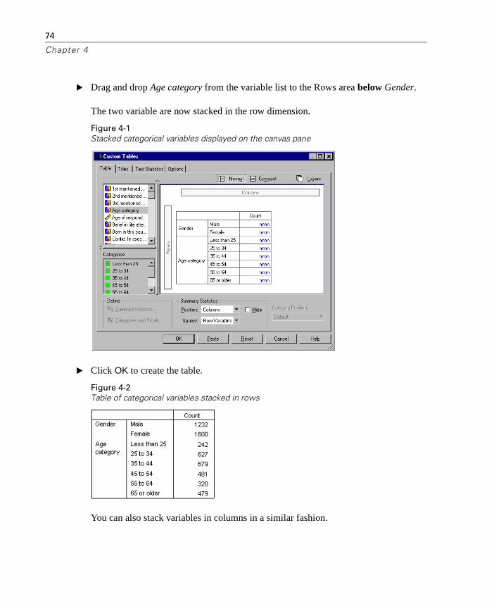
74
Chapter 4
� Drag and drop Age category from the variable list to the Rows area below Gender.
The two variable are now stacked in the row dimension.
Figure 4-1Stacked categorical variables displayed on the canvas pane
� Click OK to create the table.
Figure 4-2Table of categorical variables stacked in rows
You can also stack variables in columns in a similar fashion.
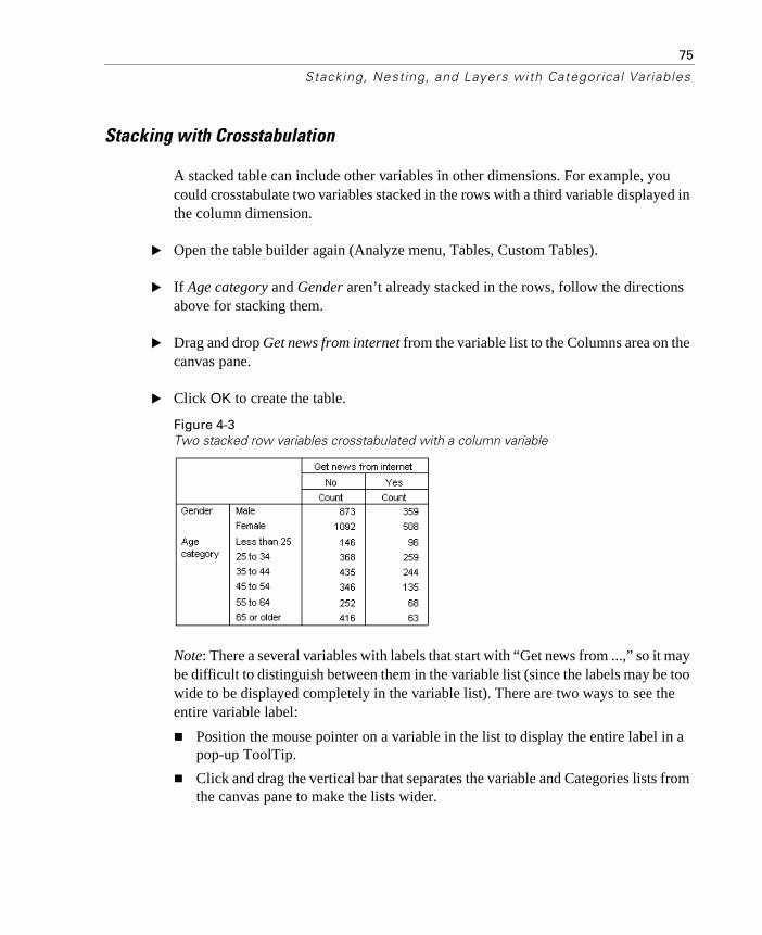
75
Stacking, Nesting, and Layers with Categorical Variables
Stacking with Crosstabulation
A stacked table can include other variables in other dimensions. For example, you could crosstabulate two variables stacked in the rows with a third variable displayed in the column dimension.
� Open the table builder again (Analyze menu, Tables, Custom Tables).
� If Age category and Gender aren’t already stacked in the rows, follow the directions above for stacking them.
� Drag and drop Get news from internet from the variable list to the Columns area on the canvas pane.
� Click OK to create the table.
Figure 4-3Two stacked row variables crosstabulated with a column variable
Note: There a several variables with labels that start with “Get news from ...,” so it may be difficult to distinguish between them in the variable list (since the labels may be too wide to be displayed completely in the variable list). There are two ways to see the entire variable label:
� Position the mouse pointer on a variable in the list to display the entire label in a pop-up ToolTip.
� Click and drag the vertical bar that separates the variable and Categories lists from the canvas pane to make the lists wider.

76
Chapter 4
Figure 4-4Variable list widened to display complete variable labels
Nesting Categorical Variables
Nesting, like crosstabulation, can show the relationship between two categorical variables, except that one variable is nested within the other in the same dimension. For example, you could nest Gender within Age category in the row dimension, showing the number of males and females in each age category.
� Open the table builder (Analyze menu, Tables, Custom Tables).
� Click Reset to delete any previous selections in the table builder.
� In the table builder, drag and drop Age category from the variable list to the Rows area on the canvas pane.
� Drag and drop Gender from the variable list to the right of Age category in the Rows area.
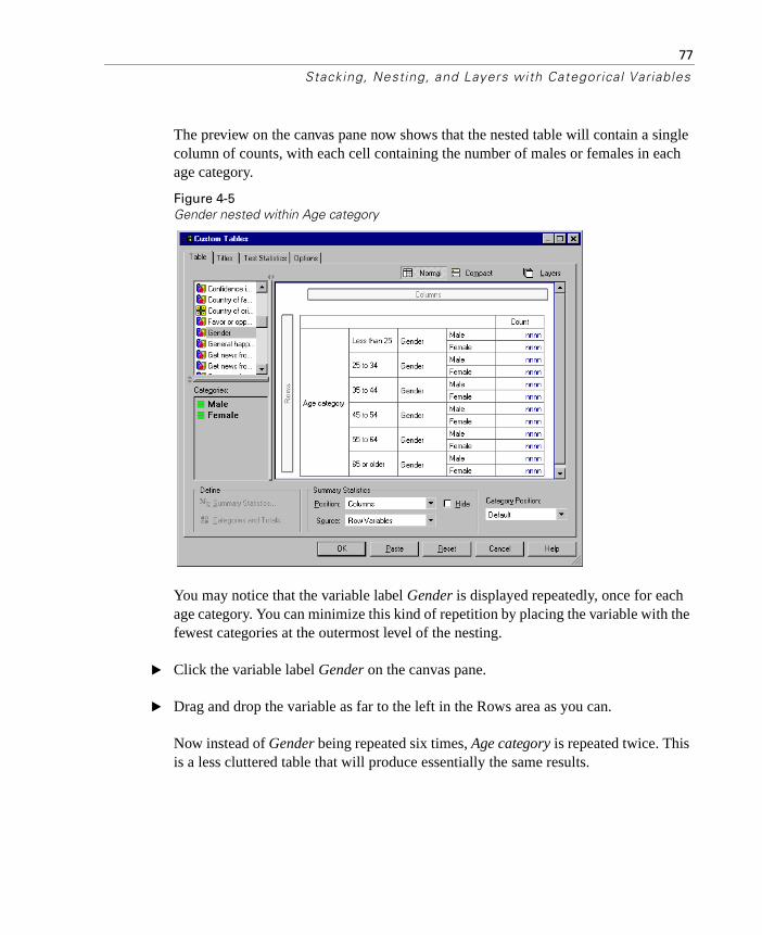
77
Stacking, Nesting, and Layers with Categorical Variables
The preview on the canvas pane now shows that the nested table will contain a single column of counts, with each cell containing the number of males or females in each age category.
Figure 4-5Gender nested within Age category
You may notice that the variable label Gender is displayed repeatedly, once for each age category. You can minimize this kind of repetition by placing the variable with the fewest categories at the outermost level of the nesting.
� Click the variable label Gender on the canvas pane.
� Drag and drop the variable as far to the left in the Rows area as you can.
Now instead of Gender being repeated six times, Age category is repeated twice. This is a less cluttered table that will produce essentially the same results.

78
Chapter 4
Figure 4-6Age category nested within Gender in table builder preview
� Click OK to create the table.
Figure 4-7Table of Age category nested within Gender

79
Stacking, Nesting, and Layers with Categorical Variables
Suppressing Variable Labels
Another solution to redundant variable labels in nested tables is simply to suppress the display of variable names or labels. Since the value labels for both Gender and Age category are probably sufficiently descriptive without the variable labels, we can eliminate the labels for both variables.
� Open the table builder (Analyze menu, Tables, Custom Tables).
� Right-click Age category on the canvas pane and deselect (uncheck) Show Variable Label on the pop-up context menu.
� Do the same for Gender.
Figure 4-8Suppressing variable labels via the context menu in the table builder
The variable labels are still displayed in the table preview, but they won’t be included in the table.
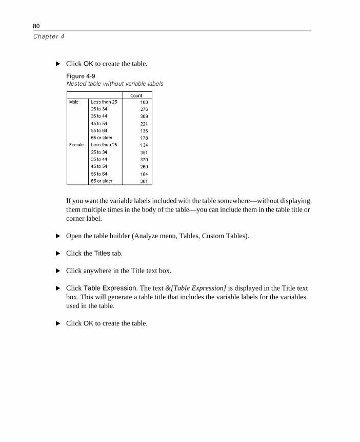
80
Chapter 4
� Click OK to create the table.
Figure 4-9Nested table without variable labels
If you want the variable labels included with the table somewhere—without displaying them multiple times in the body of the table—you can include them in the table title or corner label.
� Open the table builder (Analyze menu, Tables, Custom Tables).
� Click the Titles tab.
� Click anywhere in the Title text box.
� Click Table Expression. The text &[Table Expression] is displayed in the Title text box. This will generate a table title that includes the variable labels for the variables used in the table.
� Click OK to create the table.
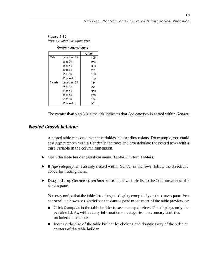
81
Stacking, Nesting, and Layers with Categorical Variables
Figure 4-10Variable labels in table title
The greater than sign (>) in the title indicates that Age category is nested within Gender.
Nested Crosstabulation
A nested table can contain other variables in other dimensions. For example, you could nest Age category within Gender in the rows and crosstabulate the nested rows with a third variable in the column dimension.
� Open the table builder (Analyze menu, Tables, Custom Tables).
� If Age category isn’t already nested within Gender in the rows, follow the directions above for nesting them.
� Drag and drop Get news from internet from the variable list to the Columns area on the canvas pane.
You may notice that the table is too large to display completely on the canvas pane. You can scroll up/down or right/left on the canvas pane to see more of the table preview, or:
� Click Compact in the table builder to see a compact view. This displays only the variable labels, without any information on categories or summary statistics included in the table.
� Increase the size of the table builder by clicking and dragging any of the sides or corners of the table builder.
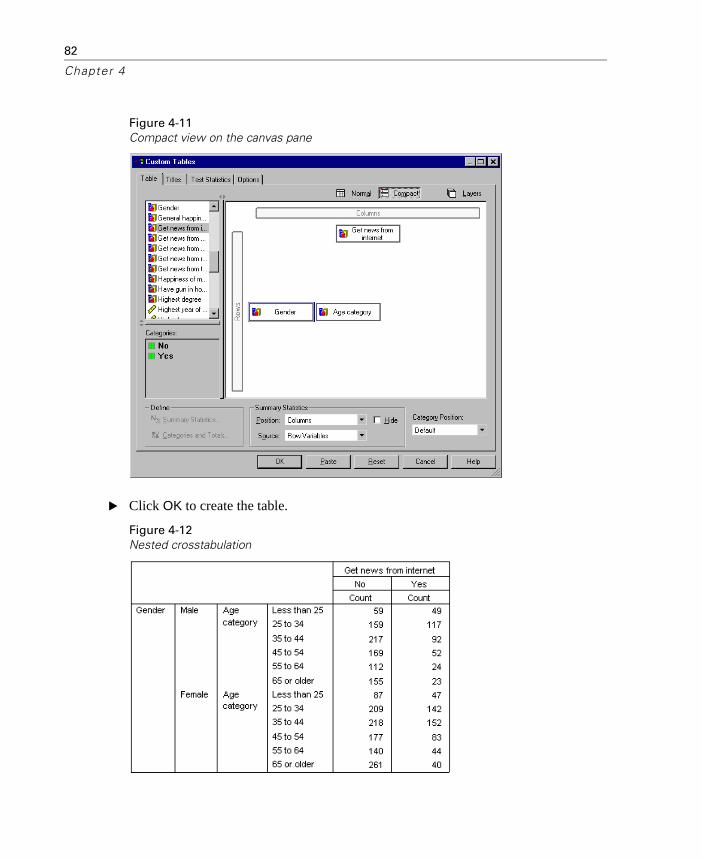
82
Chapter 4
Figure 4-11Compact view on the canvas pane
� Click OK to create the table.
Figure 4-12Nested crosstabulation

83
Stacking, Nesting, and Layers with Categorical Variables
Swapping Rows and Columns
What do you do if you spend a lot of time setting up a complex table and then decide it’s absolutely perfect—except that you want to switch the orientation, putting all of the row variables in the columns and vice versa? For example, you’ve created a nested crosstabulation with Age category and Gender nested in the rows, but now you want these two demographic variables nested in the columns instead.
� Open the table builder (Analyze menu, Tables, Custom Tables).
� Right-click anywhere on the canvas pane and select Swap Row and Column Variables from the pop-up context menu.
Figure 4-13Swapping row and column variables
The row and column variables have now been switched.
Before creating the table, let’s make a few modifications to make the display less cluttered.
� Select Hide to suppress the display of the summary statistics column label.
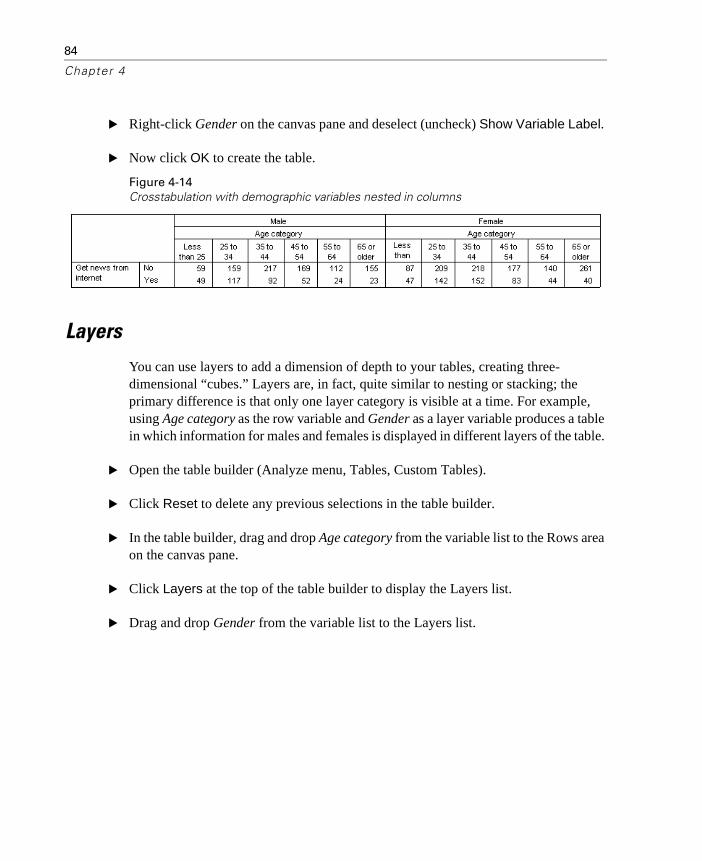
84
Chapter 4
� Right-click Gender on the canvas pane and deselect (uncheck) Show Variable Label.
� Now click OK to create the table.
Figure 4-14Crosstabulation with demographic variables nested in columns
Layers
You can use layers to add a dimension of depth to your tables, creating three-dimensional “cubes.” Layers are, in fact, quite similar to nesting or stacking; the primary difference is that only one layer category is visible at a time. For example, using Age category as the row variable and Gender as a layer variable produces a table in which information for males and females is displayed in different layers of the table.
� Open the table builder (Analyze menu, Tables, Custom Tables).
� Click Reset to delete any previous selections in the table builder.
� In the table builder, drag and drop Age category from the variable list to the Rows area on the canvas pane.
� Click Layers at the top of the table builder to display the Layers list.
� Drag and drop Gender from the variable list to the Layers list.
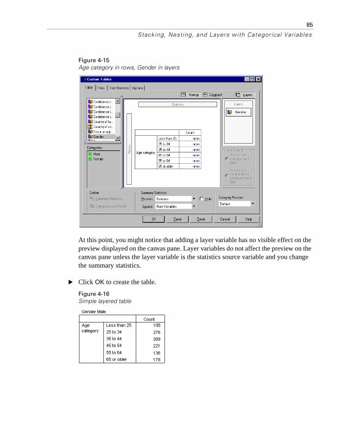
85
Stacking, Nesting, and Layers with Categorical Variables
Figure 4-15Age category in rows, Gender in layers
At this point, you might notice that adding a layer variable has no visible effect on the preview displayed on the canvas pane. Layer variables do not affect the preview on the canvas pane unless the layer variable is the statistics source variable and you change the summary statistics.
� Click OK to create the table.
Figure 4-16Simple layered table

86
Chapter 4
At first glance, this table doesn’t look any different than a simple table of a single categorical variable. The only difference is the presence of the label Gender Male at the top of the table.
� Double-click the table in the Viewer window to activate it.
� You can now see that the label Gender Male is actually a choice in a drop-down list.
� Click the down arrow on the drop-down list to display the whole list of layers.
Figure 4-17List of layers in activated pivot table
In this table, there is only one other choice in the list.
� Select Gender Female from drop-down list.
Figure 4-18Simple layered table with different layer displayed
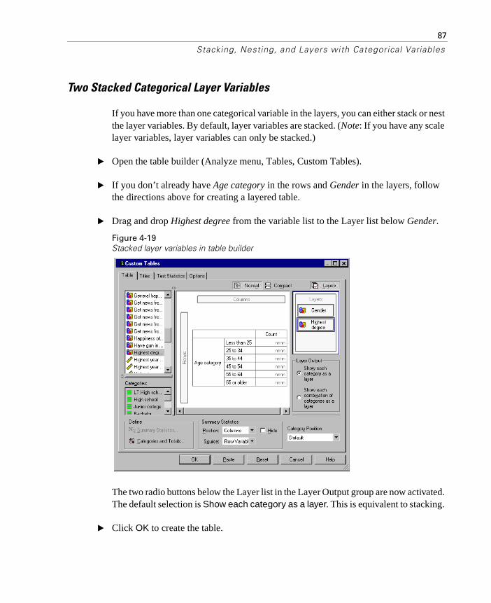
87
Stacking, Nesting, and Layers with Categorical Variables
Two Stacked Categorical Layer Variables
If you have more than one categorical variable in the layers, you can either stack or nest the layer variables. By default, layer variables are stacked. (Note: If you have any scale layer variables, layer variables can only be stacked.)
� Open the table builder (Analyze menu, Tables, Custom Tables).
� If you don’t already have Age category in the rows and Gender in the layers, follow the directions above for creating a layered table.
� Drag and drop Highest degree from the variable list to the Layer list below Gender.
Figure 4-19Stacked layer variables in table builder
The two radio buttons below the Layer list in the Layer Output group are now activated. The default selection is Show each category as a layer. This is equivalent to stacking.
� Click OK to create the table.
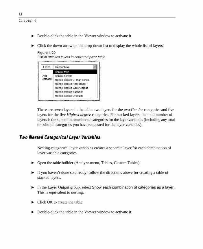
88
Chapter 4
� Double-click the table in the Viewer window to activate it.
� Click the down arrow on the drop-down list to display the whole list of layers.
Figure 4-20List of stacked layers in activated pivot table
There are seven layers in the table: two layers for the two Gender categories and five layers for the five Highest degree categories. For stacked layers, the total number of layers is the sum of the number of categories for the layer variables (including any total or subtotal categories you have requested for the layer variables).
Two Nested Categorical Layer Variables
Nesting categorical layer variables creates a separate layer for each combination of layer variable categories.
� Open the table builder (Analyze menu, Tables, Custom Tables).
� If you haven’t done so already, follow the directions above for creating a table of stacked layers.
� In the Layer Output group, select Show each combination of categories as a layer. This is equivalent to nesting.
� Click OK to create the table.
� Double-click the table in the Viewer window to activate it.

89
Stacking, Nesting, and Layers with Categorical Variables
� Click the down arrow on the drop-down list to display the whole list of layers.
Figure 4-21List of nested layers in activated pivot table
There are 10 layers in the table (you have to scroll through the list to see all of them), one for each combination of Gender and Highest degree. For nested layers, the total number of layers is the product of the number of categories for each layer variable (in this example, ).
Printing Layered Tables
By default, only the currently visible layer is printed. To print all layers of a table:
� Double-click the table in the Viewer window to activate it.
� From the Viewer window menus, choose
Format Table Properties...
� Click the Printing tab.
� Select Print all layers.
You can also save this setting as part of a TableLook, including the default TableLook.
5 2× 10=


91
Chapte r
5Totals and Subtotals for Categorical Variables
You can include both totals and subtotals in custom tables. Totals and subtotals can be applied to categorical variables at any nesting level in any dimension—row, column, and layer.
Sample Data File
The examples in this chapter use the data file survey_sample.sav. This file is located in the tutorial\sample_files folder within the folder in which SPSS is installed.
All examples provided here display variable labels in dialog boxes, sorted in alphabetical order. Variable list display properties are set on the General tab in the Options dialog box (Edit menu, Options).
Simple Total for a Single Variable
� From the menus, choose:
Analyze Tables
Custom Tables...
� In the table builder, drag and drop Age category from the variable list to the Rows area on the canvas pane.
� Right-click on Age category on the canvas pane and select Summary Statistics from the pop-up context menu.

92
Chapter 5
� In the Summary Statistics dialog box, select Column % in the Statistics list and click the arrow to add it to the Display list.
� In the Label cell in the Display list, delete the default label and type Percent.
� Click Continue.
� Right-click on Age category on the canvas pane and select Categories and Totals from the pop-up context menu.
� Select (click) Total in the Categories and Totals dialog box.
Figure 5-1Categories and Totals dialog box
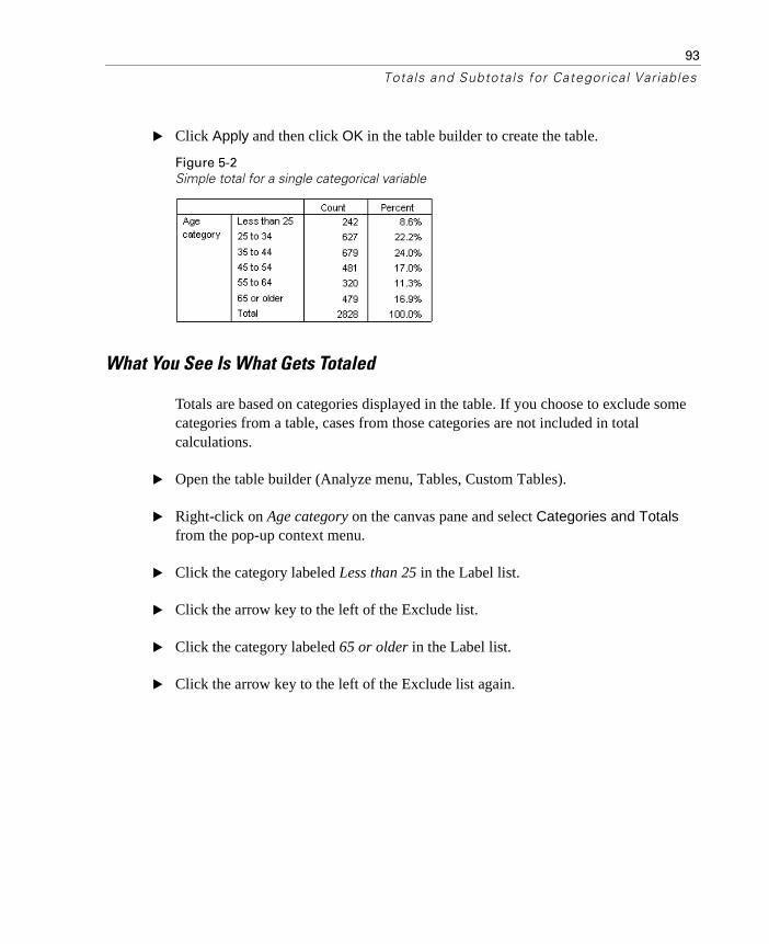
93
Totals and Subtotals for Categorical Variables
� Click Apply and then click OK in the table builder to create the table.
Figure 5-2Simple total for a single categorical variable
What You See Is What Gets Totaled
Totals are based on categories displayed in the table. If you choose to exclude some categories from a table, cases from those categories are not included in total calculations.
� Open the table builder (Analyze menu, Tables, Custom Tables).
� Right-click on Age category on the canvas pane and select Categories and Totals from the pop-up context menu.
� Click the category labeled Less than 25 in the Label list.
� Click the arrow key to the left of the Exclude list.
� Click the category labeled 65 or older in the Label list.
� Click the arrow key to the left of the Exclude list again.
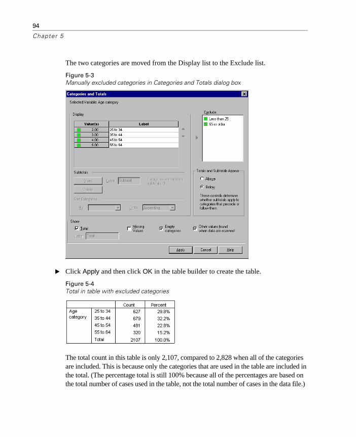
94
Chapter 5
The two categories are moved from the Display list to the Exclude list.
Figure 5-3Manually excluded categories in Categories and Totals dialog box
� Click Apply and then click OK in the table builder to create the table.
Figure 5-4Total in table with excluded categories
The total count in this table is only 2,107, compared to 2,828 when all of the categories are included. This is because only the categories that are used in the table are included in the total. (The percentage total is still 100% because all of the percentages are based on the total number of cases used in the table, not the total number of cases in the data file.)
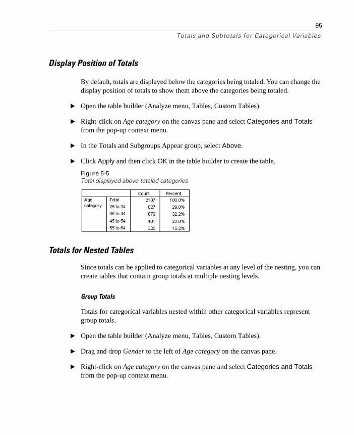
95
Totals and Subtotals for Categorical Variables
Display Position of Totals
By default, totals are displayed below the categories being totaled. You can change the display position of totals to show them above the categories being totaled.
� Open the table builder (Analyze menu, Tables, Custom Tables).
� Right-click on Age category on the canvas pane and select Categories and Totals from the pop-up context menu.
� In the Totals and Subgroups Appear group, select Above.
� Click Apply and then click OK in the table builder to create the table.
Figure 5-5Total displayed above totaled categories
Totals for Nested Tables
Since totals can be applied to categorical variables at any level of the nesting, you can create tables that contain group totals at multiple nesting levels.
Group Totals
Totals for categorical variables nested within other categorical variables represent group totals.
� Open the table builder (Analyze menu, Tables, Custom Tables).
� Drag and drop Gender to the left of Age category on the canvas pane.
� Right-click on Age category on the canvas pane and select Categories and Totals from the pop-up context menu.
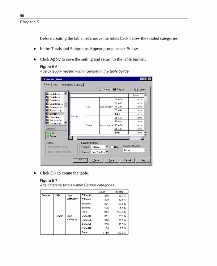
96
Chapter 5
Before creating the table, let’s move the totals back below the totaled categories.
� In the Totals and Subgroups Appear group, select Below.
� Click Apply to save the setting and return to the table builder.
Figure 5-6Age category nested within Gender in the table builder
� Click OK to create the table.
Figure 5-7Age category totals within Gender categories
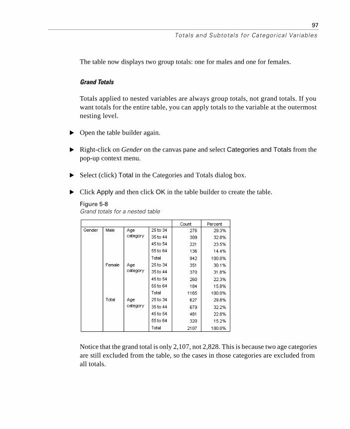
97
Totals and Subtotals for Categorical Variables
The table now displays two group totals: one for males and one for females.
Grand Totals
Totals applied to nested variables are always group totals, not grand totals. If you want totals for the entire table, you can apply totals to the variable at the outermost nesting level.
� Open the table builder again.
� Right-click on Gender on the canvas pane and select Categories and Totals from the pop-up context menu.
� Select (click) Total in the Categories and Totals dialog box.
� Click Apply and then click OK in the table builder to create the table.
Figure 5-8Grand totals for a nested table
Notice that the grand total is only 2,107, not 2,828. This is because two age categories are still excluded from the table, so the cases in those categories are excluded from all totals.

98
Chapter 5
Layer Variable Totals
Totals for layer variables are displayed as separate layers in the table.
� Open the table builder (Analyze menu, Tables, Custom Tables).
� Click Layers in the table builder to display the Layers list.
� Drag and drop Gender from the row area on the canvas pane to the Layers list.
Figure 5-9Layer variable in table builder
Note: Since you already specified totals for Gender, you don’t need to do so now. Moving the variable between dimensions does not affect any of the settings for that variable.
� Click OK to create the table.

99
Totals and Subtotals for Categorical Variables
� Double-click the table in the Viewer to activate it.
� Click the down arrow in the Layer drop-down list to display a list of all the layers in the table.
There are three layers in the table: Gender Male, Gender Female, and Gender Total.
Figure 5-10Total layer in Layer list in activated pivot table
Display Position of Layer Totals
For layer variable totals, the display position (above or below) for totals determines the layer position for the totals. For example, if you specify Above for a layer variable total, the total layer is the first layer displayed.
Subtotals
You can include subtotals for subsets of categories of a variable. For example, you could include subtotals for age categories that represent all of the respondents in the sample survey under and over age 45.
� Open the table builder (Analyze menu, Tables, Custom Tables).
� Click Reset to clear any previous settings in the table builder.
� In the table builder, drag and drop Age category from the variable list to the Rows area on the canvas pane.
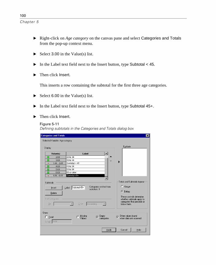
100
Chapter 5
� Right-click on Age category on the canvas pane and select Categories and Totals from the pop-up context menu.
� Select 3.00 in the Value(s) list.
� In the Label text field next to the Insert button, type Subtotal < 45.
� Then click Insert.
This inserts a row containing the subtotal for the first three age categories.
� Select 6.00 in the Value(s) list.
� In the Label text field next to the Insert button, type Subtotal 45+.
� Then click Insert.
Figure 5-11Defining subtotals in the Categories and Totals dialog box
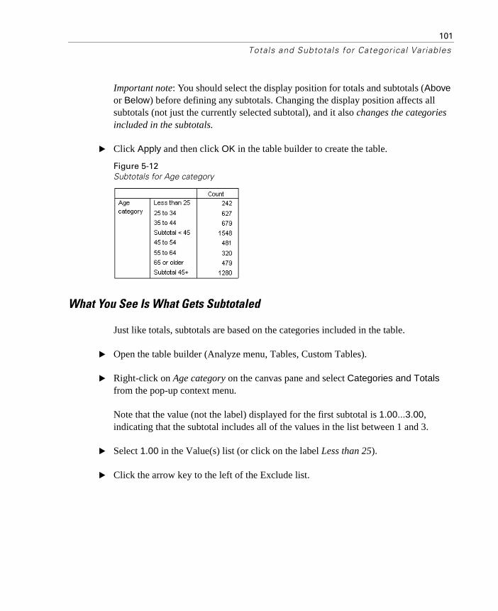
101
Totals and Subtotals for Categorical Variables
Important note: You should select the display position for totals and subtotals (Above or Below) before defining any subtotals. Changing the display position affects all subtotals (not just the currently selected subtotal), and it also changes the categories included in the subtotals.
� Click Apply and then click OK in the table builder to create the table.
Figure 5-12Subtotals for Age category
What You See Is What Gets Subtotaled
Just like totals, subtotals are based on the categories included in the table.
� Open the table builder (Analyze menu, Tables, Custom Tables).
� Right-click on Age category on the canvas pane and select Categories and Totals from the pop-up context menu.
Note that the value (not the label) displayed for the first subtotal is 1.00...3.00, indicating that the subtotal includes all of the values in the list between 1 and 3.
� Select 1.00 in the Value(s) list (or click on the label Less than 25).
� Click the arrow key to the left of the Exclude list.

102
Chapter 5
Figure 5-13Subtotals when categories are excluded
The first age category is now excluded, and the value displayed for the first subtotal changes to 2.00...3.00, indicating the fact that the excluded category will not be included in the subtotal because subtotals are based on the categories included in the table. Excluding a category automatically excludes it from any subtotals, so you cannot, for example, display only subtotals without the categories on which the subtotals are based.
Layer Variable Subtotals
Just like totals, subtotals for layer variables are displayed as separate layers in the table. Essentially, the subtotals are treated as categories. Each category is a separate layer in the table, and the display order of the layer categories is determined by the category order specified in the Categories and Totals dialog box, including the display position of the subtotal categories.
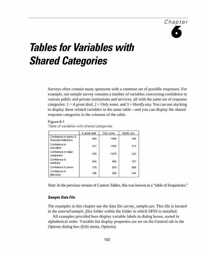
103
Chapte r
6Tables for Variables with Shared Categories
Surveys often contain many questions with a common set of possible responses. For example, our sample survey contains a number of variables concerning confidence in various public and private institutions and services, all with the same set of response categories: 1 = A great deal, 2 = Only some, and 3 = Hardly any. You can use stacking to display these related variables in the same table—and you can display the shared response categories in the columns of the table.
Figure 6-1Table of variables with shared categories
Note: In the previous version of Custom Tables, this was known as a “table of frequencies.”
Sample Data File
The examples in this chapter use the data file survey_sample.sav. This file is located in the tutorial\sample_files folder within the folder in which SPSS is installed.
All examples provided here display variable labels in dialog boxes, sorted in alphabetical order. Variable list display properties are set on the General tab in the Options dialog box (Edit menu, Options).

104
Chapter 6
Table of Counts
� From the menus, choose:
Analyze Tables
Custom Tables...
� In the variable list in the table builder, click Confidence in banks... and then Shift-click Confidence in television to select all of the “confidence” variables. (Note: This assumes that variable labels are displayed in alphabetical order, not file order, in the variable list.)
� Drag and drop the six confidence variables to the Rows area on the canvas pane.
Figure 6-2Confidence variables stacked in rows

105
Tables for Variables with Shared Categories
This stacks the variables in the row dimension. By default, the category labels for each variable are also displayed in the rows, resulting in a very long, narrow table ( )—but since all six variables share the same defined category labels (value labels), you can put the category labels in the column dimension.
� From the Category Position drop-down list, select Row Labels in Columns.
� Now the table has only six rows, one for each of the stacked variables, and the defined categories become columns in the table.
� Before creating the table, select (click) Hide for Position in the Summary Statistics group, since the summary statistic label Count isn’t really necessary.
Figure 6-3Category labels in columns
� Click OK to create the table.
6 variables 3 categories× 18 rows=
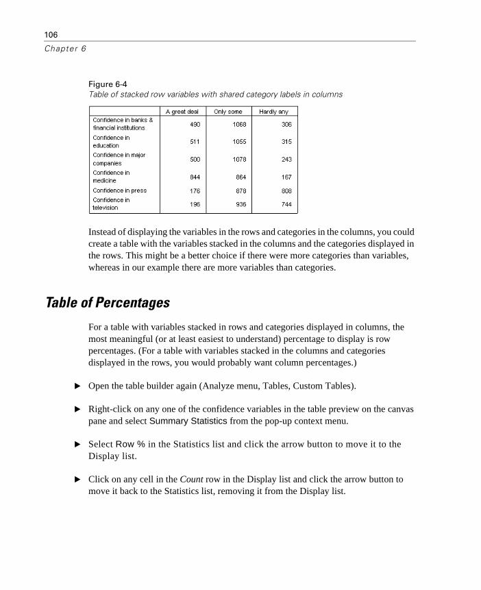
106
Chapter 6
Figure 6-4Table of stacked row variables with shared category labels in columns
Instead of displaying the variables in the rows and categories in the columns, you could create a table with the variables stacked in the columns and the categories displayed in the rows. This might be a better choice if there were more categories than variables, whereas in our example there are more variables than categories.
Table of Percentages
For a table with variables stacked in rows and categories displayed in columns, the most meaningful (or at least easiest to understand) percentage to display is row percentages. (For a table with variables stacked in the columns and categories displayed in the rows, you would probably want column percentages.)
� Open the table builder again (Analyze menu, Tables, Custom Tables).
� Right-click on any one of the confidence variables in the table preview on the canvas pane and select Summary Statistics from the pop-up context menu.
� Select Row % in the Statistics list and click the arrow button to move it to the Display list.
� Click on any cell in the Count row in the Display list and click the arrow button to move it back to the Statistics list, removing it from the Display list.

107
Tables for Variables with Shared Categories
Figure 6-5Row percentages selected in Summary Statistics dialog box
� Click Apply to All to apply the summary statistic change to all of the stacked variables in the table.
Figure 6-6Row percentages in table preview on canvas pane
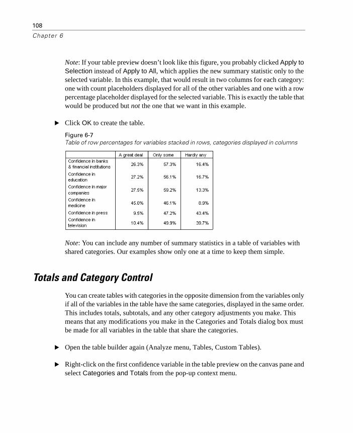
108
Chapter 6
Note: If your table preview doesn’t look like this figure, you probably clicked Apply to Selection instead of Apply to All, which applies the new summary statistic only to the selected variable. In this example, that would result in two columns for each category: one with count placeholders displayed for all of the other variables and one with a row percentage placeholder displayed for the selected variable. This is exactly the table that would be produced but not the one that we want in this example.
� Click OK to create the table.
Figure 6-7Table of row percentages for variables stacked in rows, categories displayed in columns
Note: You can include any number of summary statistics in a table of variables with shared categories. Our examples show only one at a time to keep them simple.
Totals and Category Control
You can create tables with categories in the opposite dimension from the variables only if all of the variables in the table have the same categories, displayed in the same order. This includes totals, subtotals, and any other category adjustments you make. This means that any modifications you make in the Categories and Totals dialog box must be made for all variables in the table that share the categories.
� Open the table builder again (Analyze menu, Tables, Custom Tables).
� Right-click on the first confidence variable in the table preview on the canvas pane and select Categories and Totals from the pop-up context menu.

109
Tables for Variables with Shared Categories
� Select (check) Total in the Categories and Totals dialog box and then click Apply.
Figure 6-8Probably not the results you want
The first thing you’ll probably notice is that the category labels have moved from the columns back to the rows. You may also notice that the Category Position control is now disabled. This is because the variables no longer share the exact same set of “categories.” One of the variables now has a total category.
� Right-click any one of the confidence variables on the canvas pane and select Select All Row Variables from the pop-up context menu—or Ctrl-click each stacked variable on the canvas pane until they are all selected (you may have to scroll down the pane or expand the table builder window).
� Click Categories and Totals in the Define group.
� If Total isn’t already selected (checked) in the Categories and Totals dialog box, select it now and then click Apply.

110
Chapter 6
� The Category Position drop-down list should be enabled again, since now all of the variables have the additional total category, so you can now select Row Labels in Columns.
Figure 6-9Categories and totals in columns
� Click OK to create the table.
Figure 6-10Table of row percentages for variables stacked in rows, categories and totals displayed in columns

111
Tables for Variables with Shared Categories
Nesting in Tables with Shared Categories
In nested tables, the stacked variables with the shared categories must be at the innermost nesting level of their dimension if you want to display the category labels in the opposite dimension.
� Open the table builder again (Analyze menu, Tables, Custom Tables).
� Drag and drop Gender from the variable list to the left side of the Rows area.
Figure 6-11Nested variables with shared categories
The stacked variables with shared categories are now nested within gender categories in the table preview.
� Now drag and drop Gender to the right of one of the stacked confidence variables in the table preview.

112
Chapter 6
Figure 6-12Another example of results you probably do not want
Once again, the category labels have reverted back to the row dimension, and the Category Position control is disabled. You now have one stacked variable that also has Gender nested within it, while the other stacked variables contain no nested variables. You could add Gender as a nested variable to each of the stacked variables, but then moving row labels to columns would result in the category labels for Gender being displayed in the columns, not the category labels for the stacked variables with the shared categories. This is because Gender would now be the innermost nested variable, and changing the category position always applies to the innermost nested variable.
113
Chapte r
7Summary Statistics
Summary statistics include everything from simple counts for categorical variables to measures of dispersion, such as the standard error of the mean for scale variables. It does not include significance tests available on the Test Statistics tab in the Custom Tables dialog box. Significance tests are covered in the chapter Test Statistics.
Summary statistics for categorical variables and multiple response sets include counts and a wide variety of percentage calculations, including:
� Row percentages
� Column percentages
� Subtable percentages
� Table percentages
� Valid N percentages
In addition to the summary statistics available for categorical variables, summary statistics for scale variables and custom total summaries for categorical variables include:
� Mean
� Median
� Percentiles
� Sum
� Standard deviation
� Range
� Minimum and maximum values
114
Chapter 7
Additional summary statistics are available for multiple response sets. For more information, see “Counts, Responses, Percentages, and Totals” in the chapter Multiple Response Sets. For a complete list of summary statistics see “Summary Statistics” in the chapter Table Builder Interface.
Sample Data File
The examples in this chapter use the data file survey_sample.sav. This file is located in the tutorial\sample_files folder within the folder in which SPSS is installed.
All examples provided here display variable labels in dialog boxes, sorted in alphabetical order. Variable list display properties are set on the General tab in the Options dialog box (Edit menu, Options).
Summary Statistics Source Variable
Available summary statistics depend on the measurement level of the summary statistics source variable. The source of summary statistics (the variable on which the summary statistics are based) is determined by:
� Measurement level. If a table (or a table section in a stacked table) contains a scale variable, summary statistics are based on the scale variable.
� Variable selection order. The default statistics source dimension (row or column) for categorical variables is based on the order in which you drag and drop variables onto the canvas pane. For example, if you drag a variable to the rows area first, the row dimension is the default statistics source dimension.
� Nesting. For categorical variables, summary statistics are based on the innermost variable in the statistics source dimension.
A stacked table may have multiple summary statistics source variables (both scale and categorical), but each table section has only one summary statistics source.
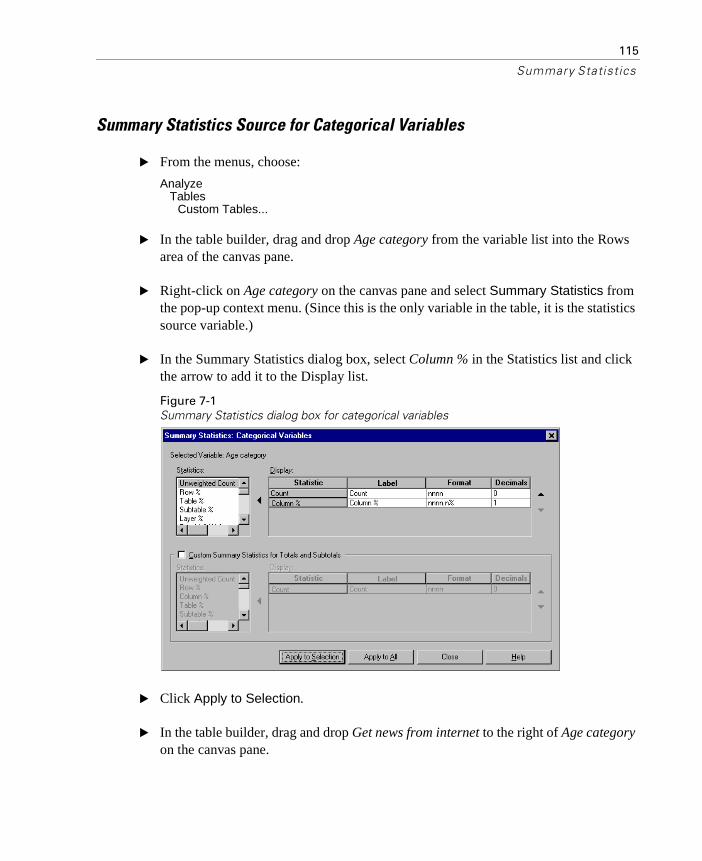
115
Summary Statist ics
Summary Statistics Source for Categorical Variables
� From the menus, choose:
Analyze Tables
Custom Tables...
� In the table builder, drag and drop Age category from the variable list into the Rows area of the canvas pane.
� Right-click on Age category on the canvas pane and select Summary Statistics from the pop-up context menu. (Since this is the only variable in the table, it is the statistics source variable.)
� In the Summary Statistics dialog box, select Column % in the Statistics list and click the arrow to add it to the Display list.
Figure 7-1Summary Statistics dialog box for categorical variables
� Click Apply to Selection.
� In the table builder, drag and drop Get news from internet to the right of Age category on the canvas pane.

116
Chapter 7
Figure 7-2Nested categorical variables
� Right-click on Age category on the canvas pane again. The Summary Statistics item on the context menu is now disabled, because Age category is not the innermost nested variable in the statistics source dimension.
� Right click on Get news from internet on the canvas pane. The Summary Statistics item is enabled because this is now the summary statistics source variable, because it is the innermost nested variable in the statistics source dimension. (Since the table has only one dimension—rows—it is the statistics source dimension.)
� Drag and drop Get news from internet from the Rows area on the canvas pane into the Columns area.

117
Summary Statist ics
Figure 7-3Crosstabulated categorical variables
� Right-click on Get news from internet on the canvas pane again. The Summary Statistics item on the pop-up context menu is now disabled, because the variable is no longer in the statistics source dimension.
Age category is once again the statistics source variable, because the default statistics source dimension for categorical variables is the first dimension where you put variables when creating the table. In this example, the first thing we did was put variables in the row dimension. Thus, the row dimension is the default statistics source dimension; and since Age category is now the only variable in that dimension, it is the statistics source variable.
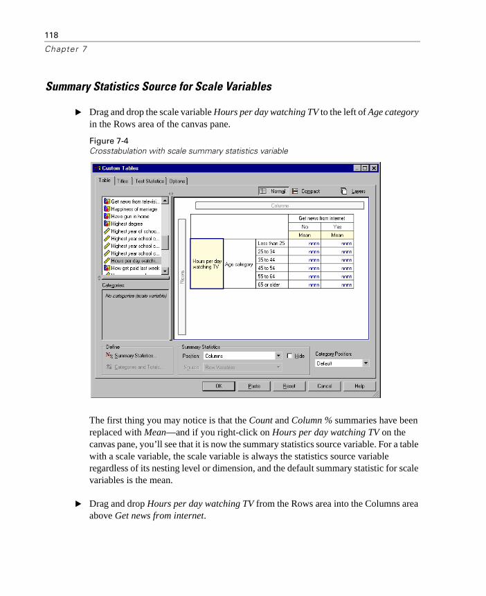
118
Chapter 7
Summary Statistics Source for Scale Variables
� Drag and drop the scale variable Hours per day watching TV to the left of Age category in the Rows area of the canvas pane.
Figure 7-4Crosstabulation with scale summary statistics variable
The first thing you may notice is that the Count and Column % summaries have been replaced with Mean—and if you right-click on Hours per day watching TV on the canvas pane, you’ll see that it is now the summary statistics source variable. For a table with a scale variable, the scale variable is always the statistics source variable regardless of its nesting level or dimension, and the default summary statistic for scale variables is the mean.
� Drag and drop Hours per day watching TV from the Rows area into the Columns area above Get news from internet.
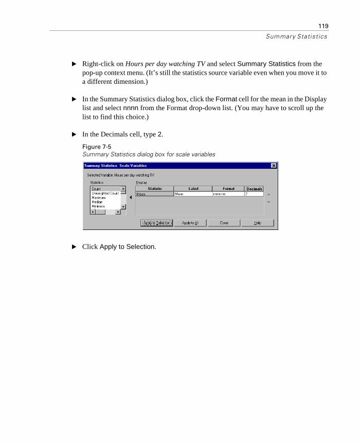
119
Summary Statist ics
� Right-click on Hours per day watching TV and select Summary Statistics from the pop-up context menu. (It’s still the statistics source variable even when you move it to a different dimension.)
� In the Summary Statistics dialog box, click the Format cell for the mean in the Display list and select nnnn from the Format drop-down list. (You may have to scroll up the list to find this choice.)
� In the Decimals cell, type 2.
Figure 7-5Summary Statistics dialog box for scale variables
� Click Apply to Selection.

120
Chapter 7
Figure 7-6Scale summary statistic with two decimals
The table preview on the canvas pane now shows that the mean values will be displayed with two decimals.
� Click OK to create the table.
Figure 7-7Scale variable summarized within crosstabulated categorical variables

121
Summary Statist ics
Stacked Variables
Since a stacked table can contain multiple statistics source variables, and you can specify different summary statistics for each of those statistics source variables, there are a few special considerations for specifying summary statistics in stacked tables.
� Open the table builder (Analyze menu, Tables, Custom Tables).
� Click Reset to clear any previous settings in the table builder.
� Click Get news from internet in the variable list and then shift-click Get news from television in the variable list to select all of the “news” variables. (Note: This assumes that variable labels are displayed in alphabetical order, not file order, in the variable list.)
� Drag and drop the five news variables into the Rows area of the canvas pane.
Figure 7-8News variables stacked in rows
The five news variables are stacked in the row dimension.

122
Chapter 7
� Click Get news from internet on the canvas pane so that only that variable is selected.
� Now right-click Get news from internet and select Summary Statistics from the pop-up context menu.
� In the Summary Statistics dialog box, select Column% from the Statistics list and click the arrow to add it to the Display list. (You can use the arrow to move selected statistics from the Statistics list into the Display list, or you can drag and drop selected statistics from the Statistics list into the Display list.)
� Then click Apply to Selection.
Figure 7-9Additional statistic applied to one variable in a stacked table
A column is added for column percentages—but the table preview on the canvas pane indicates that column percentages will be displayed for only one variable. This is because in a stacked table there are multiple statistics source variables, and each one
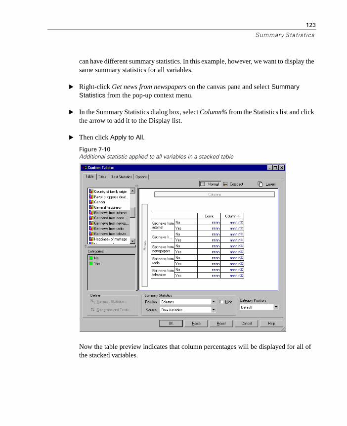
123
Summary Statist ics
can have different summary statistics. In this example, however, we want to display the same summary statistics for all variables.
� Right-click Get news from newspapers on the canvas pane and select Summary Statistics from the pop-up context menu.
� In the Summary Statistics dialog box, select Column% from the Statistics list and click the arrow to add it to the Display list.
� Then click Apply to All.
Figure 7-10Additional statistic applied to all variables in a stacked table
Now the table preview indicates that column percentages will be displayed for all of the stacked variables.

124
Chapter 7
Custom Total Summary Statistics for Categorical Variables
For categorical statistics source variables, you can include custom total summary statistics that are different from the statistics displayed for the categories of the variable. For example, for an ordinal variable, you could display percentages for each category and the mean or median for the custom total summary statistic.
� Open the table builder (Analyze menu, Tables, Custom Tables).
� Click Reset to clear any previous settings in the table builder.
� Click Confidence in press in the variable list, and then Ctrl-click Confidence in TV to select both variables.
� Drag and drop the two variables into the Rows area of the canvas pane. This stacks the two variables in the row dimension.
� Right-click either variable on the canvas pane and select Select All Row Variables from the pop-up context menu. (They may both already be selected, but we want to make sure.)
� Right-click the variable again and select Categories and Totals from the pop-up context menu.
� In the Categories and Totals dialog box, click (check) Total, and then click Apply.
The table preview on the canvas pane now displays a total row for both variables. In order to display custom total summary statistics, totals and/or subtotals must be specified for the table.
� Right-click either variable on the canvas pane and select Summary Statistics from the pop-up context menu.
� In the Summary Statistics dialog box, click Count in the Display list and click the arrow to move it to the Statistics list, removing it from the Display list.

125
Summary Statist ics
� Click Column% in the Statistics list and click the arrow key to move it to the Display list.
� Click (check) Custom Summary Statistics for Totals and Subtotals.
� Click Count in the custom summary Display list and click the arrow to move it to the custom summary Statistics list, removing it from the Display list.
� Click Mean in the custom summary Statistics list and click the arrow to move it to the custom summary Display list.
� Click the Format cell for the mean in the Display list and select nnnn from the drop-down list of formats. (You may have to scroll up the list to find this choice.)
� In the Decimals cell, type 2.
Figure 7-11Selecting custom summary statistics for totals

126
Chapter 7
� Click Apply to All to apply these settings to both variables in the table.
Figure 7-12Custom total summary statistics for row variables displayed in columns
A new column has been added for the custom total summary statistic, which may not be what you want, since the preview on the canvas pane clearly indicates that this will result in a table with many empty cells.
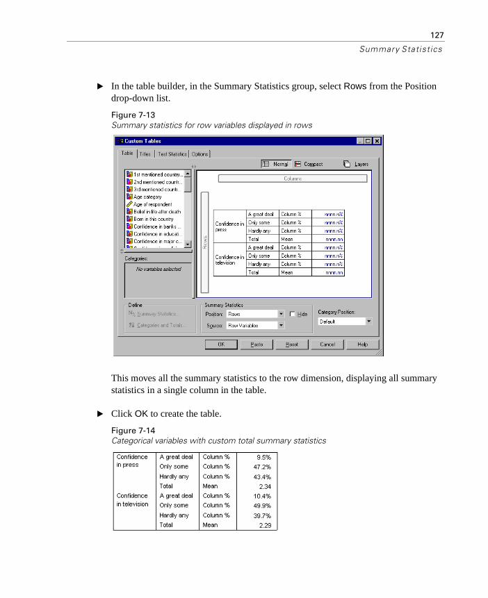
127
Summary Statist ics
� In the table builder, in the Summary Statistics group, select Rows from the Position drop-down list.
Figure 7-13Summary statistics for row variables displayed in rows
This moves all the summary statistics to the row dimension, displaying all summary statistics in a single column in the table.
� Click OK to create the table.
Figure 7-14Categorical variables with custom total summary statistics

128
Chapter 7
Displaying Category Values
There’s only one small problem with the preceding table—it may be hard to interpret the mean value without knowing the underlying category values on which it is based. Is a mean of 2.34 somewhere between A great deal and Only some—or is it somewhere between Only some and Hardly any?
Although we can’t address this problem directly in Custom Tables, we can address it in a more general way.
� From the menus, choose:
Edit Options...
� In the Options dialog box, click the Output Labels tab.
� In the Pivot Table Labeling group, select Values and Labels from the Variable values in labels shown as drop-down list.
Figure 7-15Output labeling options
� Click OK to save this setting.
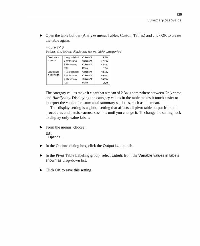
129
Summary Statist ics
� Open the table builder (Analyze menu, Tables, Custom Tables) and click OK to create the table again.
Figure 7-16Values and labels displayed for variable categories
The category values make it clear that a mean of 2.34 is somewhere between Only some and Hardly any. Displaying the category values in the table makes it much easier to interpret the value of custom total summary statistics, such as the mean.
This display setting is a global setting that affects all pivot table output from all procedures and persists across sessions until you change it. To change the setting back to display only value labels:
� From the menus, choose:
Edit Options...
� In the Options dialog box, click the Output Labels tab.
� In the Pivot Table Labeling group, select Labels from the Variable values in labels shown as drop-down list.
� Click OK to save this setting.


131
Chapte r
8Summarizing Scale Variables
A wide range of summary statistics are available for scale variables. In addition to the counts and percentages available for categorical variables, summary statistics for scale variables also include:
� Mean
� Median
� Percentiles
� Sum
� Standard deviation
� Range
� Minimum and maximum values
For more information, see “Summary Statistics for Scale Variables and Categorical Custom Totals” in the chapter Table Builder Interface.
Sample Data File
The examples in this chapter use the data file survey_sample.sav. This file is located in the tutorial\sample_files folder within the folder in which SPSS is installed.
All examples provided here display variable labels in dialog boxes, sorted in alphabetical order. Variable list display properties are set on the General tab in the Options dialog box (Edit menu, Options).

132
Chapter 8
Stacked Scale Variables
You can summarize multiple scale variables in the same table by stacking them in the table.
� From the menus, choose:
Analyze Tables
Custom Tables...
� In the table builder, click Age of respondent in the variable list, Ctrl-click Highest year of school completed, and Ctrl-click Hours per day watching TV to select all three variables.
� Drag and drop the three selected variables to the Rows area of the canvas pane.
Figure 8-1Stacked scale variables in table builder

133
Summarizing Scale Variables
The three variables are stacked in the row dimension. Since all three variables are scale variables, no categories are displayed, and the default summary statistic is the mean.
� Click OK to create the table.
Figure 8-2Table of mean values of stacked scale variables
Multiple Summary Statistics
By default, the mean is displayed for scale variables; however, you can choose other summary statistics for scale variables, and you can display more than one summary statistic.
� Open the table builder (Analyze menu, Tables, Custom Tables).
� Right-click any one of the three scale variables in the table preview on the canvas pane and select Summary Statistics from the pop-up context menu.
� In the Summary Statistics dialog box, select Median in the Statistics list and click the arrow to add it to the Display list. (You can use the arrow to move selected statistics from the Statistics list to the Display list, or you can drag and drop selected statistics from the Statistics list into the Display list.)
� Click the Format cell for the median in the Display list and select nnnn from the drop-down list of formats.
� In the Decimals cell, type 1.
� Make the same changes for the mean in the Display list.

134
Chapter 8
Figure 8-3Mean and median selected in Summary Statistics dialog box
� Click Apply to All to apply these changes to all three scale variables.
� Click OK in the table builder to create the table.
Figure 8-4Mean and median displayed in table of stacked scale variables
Count, Valid N, and Missing Values
It is often useful to display the number of cases used to compute summary statistics, such as the mean, and you might assume (not unreasonably) that the summary statistic Count would provide that information. However, this will not give you an accurate case base if there are any missing values. To obtain an accurate case base, use Valid N.
� Open the table builder (Analyze menu, Tables, Custom Tables).
� Right-click any one of the three scale variables in the table preview on the canvas pane and select Summary Statistics from the pop-up context menu.
� In the Summary Statistics dialog box, select Count in the Statistics list and click the arrow to add it to the Display list.

135
Summarizing Scale Variables
� Then select Valid N in the Statistics list and click the arrow to add it to the Display list.
� Click Apply to All to apply these changes to all three scale variables.
� Click OK in the table builder to create the table.
Figure 8-5Count versus Valid N
For all three variable, Count is the same: 2,832. Not coincidentally, this is the total number of cases in the data file. Since the scale variables aren’t nested within any categorical variables, Count simply represents the total number of cases in the data file.
Valid N, on the other hand, is different for each variable and differs quite a lot from Count for Hours per day watching TV. This is because there is a large number of missing values for this variable—that is, cases with no value recorded for this variable or values defined as representing missing data (such as a code of 99 to represent “not applicable” for pregnancy in males).
� Open the table builder (Analyze menu, Tables, Custom Tables).
� Right-click any one of the three scale variables in the table preview on the canvas pane and select Summary Statistics from the pop-up context menu.
� In the Summary Statistics dialog box, select Valid N in the Display list and click the arrow key to move it back to the Statistics list, removing it from the Display list.
� Select Count in the Display list and click the arrow key to move it back to the Statistics list, removing it from the Display list.
� Select Missing in the Statistics list and click the arrow key to add it to the Display list.
� Click Apply to All to apply these changes to all three scale variables.
� Click OK in the table builder to create the table.
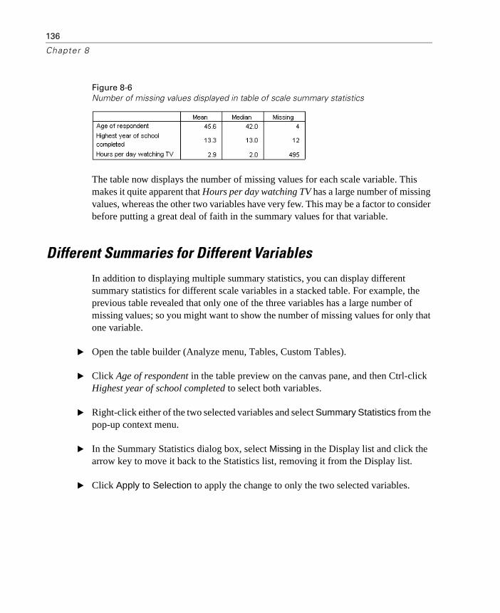
136
Chapter 8
Figure 8-6Number of missing values displayed in table of scale summary statistics
The table now displays the number of missing values for each scale variable. This makes it quite apparent that Hours per day watching TV has a large number of missing values, whereas the other two variables have very few. This may be a factor to consider before putting a great deal of faith in the summary values for that variable.
Different Summaries for Different Variables
In addition to displaying multiple summary statistics, you can display different summary statistics for different scale variables in a stacked table. For example, the previous table revealed that only one of the three variables has a large number of missing values; so you might want to show the number of missing values for only that one variable.
� Open the table builder (Analyze menu, Tables, Custom Tables).
� Click Age of respondent in the table preview on the canvas pane, and then Ctrl-click Highest year of school completed to select both variables.
� Right-click either of the two selected variables and select Summary Statistics from the pop-up context menu.
� In the Summary Statistics dialog box, select Missing in the Display list and click the arrow key to move it back to the Statistics list, removing it from the Display list.
� Click Apply to Selection to apply the change to only the two selected variables.
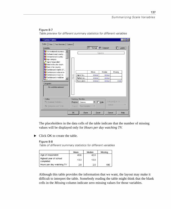
137
Summarizing Scale Variables
Figure 8-7Table preview for different summary statistics for different variables
The placeholders in the data cells of the table indicate that the number of missing values will be displayed only for Hours per day watching TV.
� Click OK to create the table.
Figure 8-8Table of different summary statistics for different variables
Although this table provides the information that we want, the layout may make it difficult to interpret the table. Somebody reading the table might think that the blank cells in the Missing column indicate zero missing values for those variables.

138
Chapter 8
� Open the table builder (Analyze menu, Tables, Custom Tables).
� In the Summary Statistics group in the table builder, select Rows from the Position drop-down list.
Figure 8-9Moving summary statistics from the column dimension to the row dimension
� Click OK to create the table.
Figure 8-10Summary statistics and variables both displayed in the row dimension
Now it’s clear that the table reports the number of missing values for only one variable.

139
Summarizing Scale Variables
Group Summaries in Categories
You can use categorical variables as grouping variables to display scale variable summaries within groups defined by the categories of the categorical variable.
� Open the table builder (Analyze menu, Tables, Custom Tables).
� Drag and drop Gender from the variable list into the Columns area of the canvas pane.
If you right-click Gender in the table preview on the canvas pane, you will see that Summary Statistics is disabled on the pop-up context menu. This is because in a table with scale variables, the scale variables are always the statistics source variables.
� Click OK to create the table.
Figure 8-11Grouped scale summaries using a categorical column variable
This table makes it easy to compare the averages (mean and median) for males and females, and it clearly shows that there isn’t much difference between them—which may not be terribly interesting but might be useful information.
Multiple Grouping Variables
You can subdivide the groups further by nesting and/or using both row and column categorical grouping variables.
� Open the table builder (Analyze menu, Tables, Custom Tables).

140
Chapter 8
� Drag and drop Get news from internet from the variable list to the far left side of the Rows area of the canvas pane. Make sure to position it so that all three scale variables are nested within it, not just one of them.
Figure 8-12Correct: All three scale variables nested within the categorical variable

141
Summarizing Scale Variables
Figure 8-13Wrong: Only one scale variable nested within the categorical variable
Although there may be times when you want something like the second example above, it’s not what we want in this case.
� Click OK to create the table.
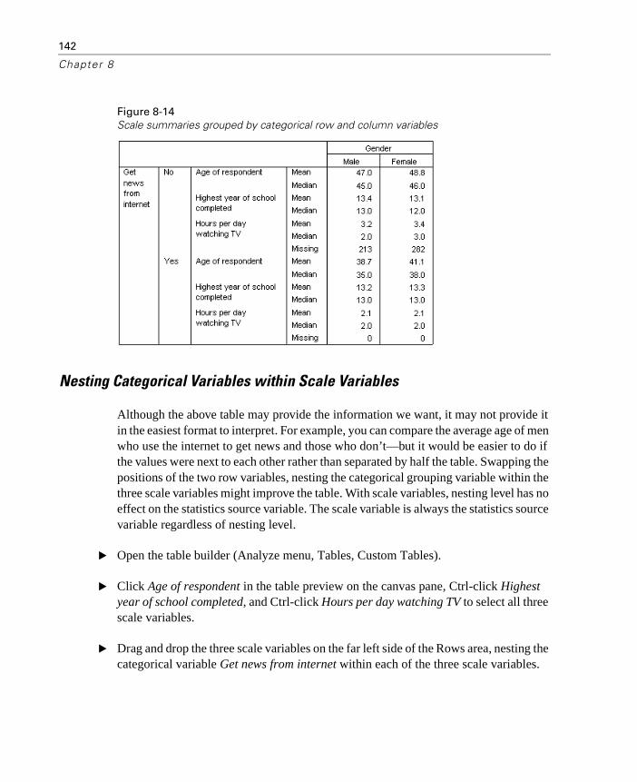
142
Chapter 8
Figure 8-14Scale summaries grouped by categorical row and column variables
Nesting Categorical Variables within Scale Variables
Although the above table may provide the information we want, it may not provide it in the easiest format to interpret. For example, you can compare the average age of men who use the internet to get news and those who don’t—but it would be easier to do if the values were next to each other rather than separated by half the table. Swapping the positions of the two row variables, nesting the categorical grouping variable within the three scale variables might improve the table. With scale variables, nesting level has no effect on the statistics source variable. The scale variable is always the statistics source variable regardless of nesting level.
� Open the table builder (Analyze menu, Tables, Custom Tables).
� Click Age of respondent in the table preview on the canvas pane, Ctrl-click Highest year of school completed, and Ctrl-click Hours per day watching TV to select all three scale variables.
� Drag and drop the three scale variables on the far left side of the Rows area, nesting the categorical variable Get news from internet within each of the three scale variables.

143
Summarizing Scale Variables
� Click OK to create the table.
Figure 8-15Categorical row variable nested within stacked scale variables
The choice of nesting order depends on the relationships or comparisons you want to emphasize in the table. Changing the nesting order of the scale variables doesn’t change the summary statistics values; it changes only their relative positions in the table.


145
Chapte r
9Test Statistics
Three different tests of significance are available for studying the relationship between row and column variables. This chapter discusses the output of each of these tests, with special attention to the effects of nesting and stacking. For more information, see the chapter Stacking, Nesting, and Layers with Categorical Variables.
Sample Data File
The examples in this chapter use the data file survey_sample.sav. This file is located in the tutorial\sample_files folder within the folder in which SPSS is installed.
Tests of Independence (Chi-Square)
The chi-square test of independence is used to determine whether there is a relationship between two categorical variables. For example, you may want to determine whether Labor force status is related to Marital status.
� From the menus, choose:
AnalyzeTables
Custom Tables...
� In the table builder, drag and drop Labor force status from the variable list into the Rows area of the canvas pane.
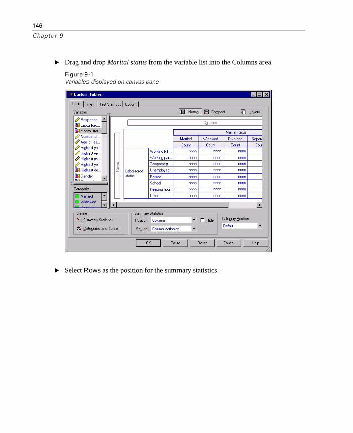
146
Chapter 9
� Drag and drop Marital status from the variable list into the Columns area.
Figure 9-1Variables displayed on canvas pane
� Select Rows as the position for the summary statistics.
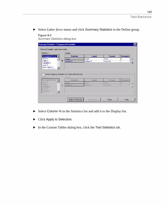
147
Test Statist ics
� Select Labor force status and click Summary Statistics in the Define group.
Figure 9-2Summary Statistics dialog box
� Select Column % in the Statistics list and add it to the Display list.
� Click Apply to Selection.
� In the Custom Tables dialog box, click the Test Statistics tab.

148
Chapter 9
Figure 9-3Test Statistics tab with the Tests of independence (chi-square) selected
� Select Tests of independence (Chi-square).
� Click OK to create the table and obtain the chi-square test.

149
Test Statist ics
Figure 9-4Labor force status by Marital status
This table is a crosstabulation of Labor force status by Marital status, with counts and column proportions shown as the summary statistics. Column proportions are computed so that they sum to 100% down each column. If these two variables are unrelated, then in each row the proportions should be similar across columns. There appear to be differences in the proportions, but you can check the chi-square test to be sure.
Figure 9-5Pearson’s chi-square test
The test of independence hypothesizes that Labor force status and Marital status are unrelated—that is, that the column proportions are the same across columns, and any observed discrepancies are due to chance variation. The chi-square statistic measures the

150
Chapter 9
overall discrepancy between the observed cell counts and the counts you would expect if the column proportions were the same across columns. A larger chi-square statistic indicates a greater discrepancy between the observed and expected cell counts—greater evidence that the column proportions are not equal, that the hypothesis of independence is incorrect, and, therefore, that Labor force status and Marital status are related.
The computed chi-square statistic has a value of 729.242. In order to determine whether this is enough evidence to reject the hypothesis of independence, the significance value of the statistic is computed. The significance value is the probability that a random variate drawn from a chi-square distribution with 28 degrees of freedom is greater than 729.242. Since this value is less than the alpha level specified on the Test Statistics tab, you can reject the hypothesis of independence at the 0.05 level. Thus, Labor force status and Marital status are in fact related.
Effects of Nesting and Stacking on Tests of Independence
The rule for tests of independence is as follows: a separate test is performed for each innermost subtable. To see how nesting affects the tests, consider the previous example, but with Marital status nested within levels of Gender.
� Open the table builder again (Analyze menu, Tables, Custom Tables).
� Drag and drop Gender from the variable list into the Columns area of the canvas pane above Marital status.
� Click OK to create the table.
Figure 9-6Pearson’s chi-square test

151
Test Statist ics
With Marital status nested within levels of Gender, two tests are performed—one for each level of Gender. The significance value for each test indicates that you can reject the hypothesis of independence between Marital status and Labor force status for both males and females. However, the table notes that more than 20% of each table’s cells have expected counts of less than 5, and the minimum expected cell count is less than 1. These notes indicate that the assumptions of the chi-square test may not be met by these tables, and so the results of the tests are suspect. The notes in this figure are numbered, rather than lettered, because this figure is formatted using the SPSS Doc TableLook instead of the default.
Note: The footnotes may be cut off from view by the cell boundaries. You can make them visible by changing the alignment of these cells in the Cell Properties dialog box.
To see how stacking affects the tests:
� Open the table builder again (Analyze menu, Tables, Custom Tables).
� Drag and drop Highest degree from the variable list into the Rows area below Labor force status.
� Click OK to create the table.
Figure 9-7Pearson’s chi-square test
152
Chapter 9
With Highest degree stacked with Labor force status, four tests are performed—a test of the independence of Marital status and Labor force status, and a test of Marital status and Highest degree for each level of Gender. The test results for Marital status and Labor force status are the same as before. The test results for Marital status and Highest degree indicate these variables are not independent.
Comparing Column Means
The column means tests are used to determine whether there is a relationship between a categorical variable in the Columns and a continuous variable in the Rows. Moreover, you can use the test results to determine the relative ordering of categories of the categorical variable in terms of the mean value of the continuous variable. For example, you may want to determine whether Hours per day watching TV is related to Get news from newspapers.
� From the menus, choose:
AnalyzeTables
Custom Tables...
� Click Reset to restore the default settings to all tabs.
� In the table builder, drag and drop Hours per day watching TV from the variable list into the Rows area of the canvas pane.
� Drag and drop Get news from newspapers from the variable list into the Columns area.

153
Test Statist ics
Figure 9-8Variables displayed on canvas pane
� Select Hours per day watching TV and click Summary Statistics in the Define group.
Figure 9-9Summary Statistics dialog box
� Select nnnn as the format.
� Select 2 as the number of decimals to display. Notice that this causes the format to now read nnnn.nn.
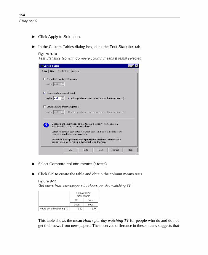
154
Chapter 9
� Click Apply to Selection.
� In the Custom Tables dialog box, click the Test Statistics tab.
Figure 9-10Test Statistics tab with Compare column means (t tests) selected
� Select Compare column means (t-tests).
� Click OK to create the table and obtain the column means tests.
Figure 9-11Get news from newspapers by Hours per day watching TV
This table shows the mean Hours per day watching TV for people who do and do not get their news from newspapers. The observed difference in these means suggests that

155
Test Statist ics
people who do not get their news from newspapers spend approximately 0.18 more hours watching TV than people who do get their news from newspapers. To see whether this difference is due to chance variation, check the column means tests.
Figure 9-12Comparisons of column means
The column means test table assigns a letter key to each category of the column variable. For Get news from newspapers, the category No is assigned the letter A, and Yes is assigned the letter B. For each pair of columns, the column means are compared using a t test. Since there are only two columns, only one test is performed. For each significant pair, the key of the category with the smaller mean is placed under the category with larger mean. Since no keys are reported in the cells of the table, this means that the column means are not statistically different.
Effects of Nesting and Stacking on Column Means Tests
The rule for column means tests is as follows: a separate set of pairwise tests is performed for each innermost subtable. To see how nesting affects the tests, consider the previous example, but with Hours per day watching TV nested within levels of Labor force status.
� Open the table builder again (Analyze menu, Tables, Custom Tables).
� Drag and drop Labor force status from the variable list into the Rows area of the canvas pane.
� Click OK to create the table.

156
Chapter 9
Figure 9-13Comparisons of column means
With Hours watching TV nested within levels of Labor force status, seven sets of column means tests are performed: one for each level of Labor force status. The same letter keys are assigned to the categories of Get news from newspapers. For respondents working full time, the B key appears in A’s column. This means that for full-time employees, the mean value of Hours per day watching TV is lower for people who get their news from newspapers. No other keys appear in the columns, so you can conclude that there are no other statistically significant differences in the column means.
Bonferroni adjustments. When multiple tests are performed, the Bonferroni adjustment is applied to column means tests to ensure that the alpha level (or false positive rate) specified on the Test Statistics tab applies to each set of tests. Thus, in this table, no Bonferroni adjustments were applied, because although seven sets of tests are performed, within each set only one pair of columns is compared.
To see how stacking affects the tests:
� Open the table builder again (Analyze menu, Tables, Custom Tables).
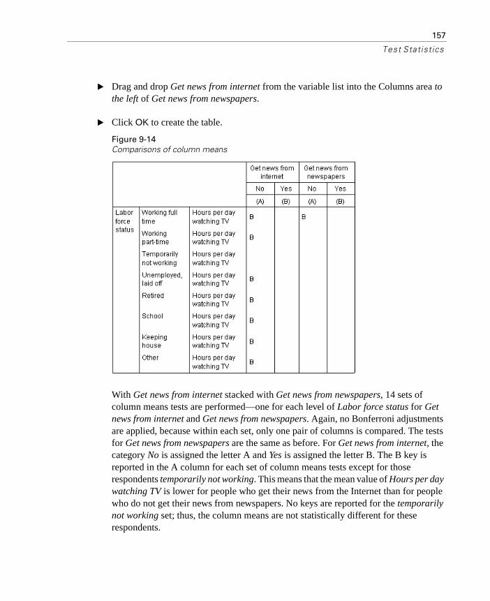
157
Test Statist ics
� Drag and drop Get news from internet from the variable list into the Columns area to the left of Get news from newspapers.
� Click OK to create the table.
Figure 9-14Comparisons of column means
With Get news from internet stacked with Get news from newspapers, 14 sets of column means tests are performed—one for each level of Labor force status for Get news from internet and Get news from newspapers. Again, no Bonferroni adjustments are applied, because within each set, only one pair of columns is compared. The tests for Get news from newspapers are the same as before. For Get news from internet, the category No is assigned the letter A and Yes is assigned the letter B. The B key is reported in the A column for each set of column means tests except for those respondents temporarily not working. This means that the mean value of Hours per day watching TV is lower for people who get their news from the Internet than for people who do not get their news from newspapers. No keys are reported for the temporarily not working set; thus, the column means are not statistically different for these respondents.
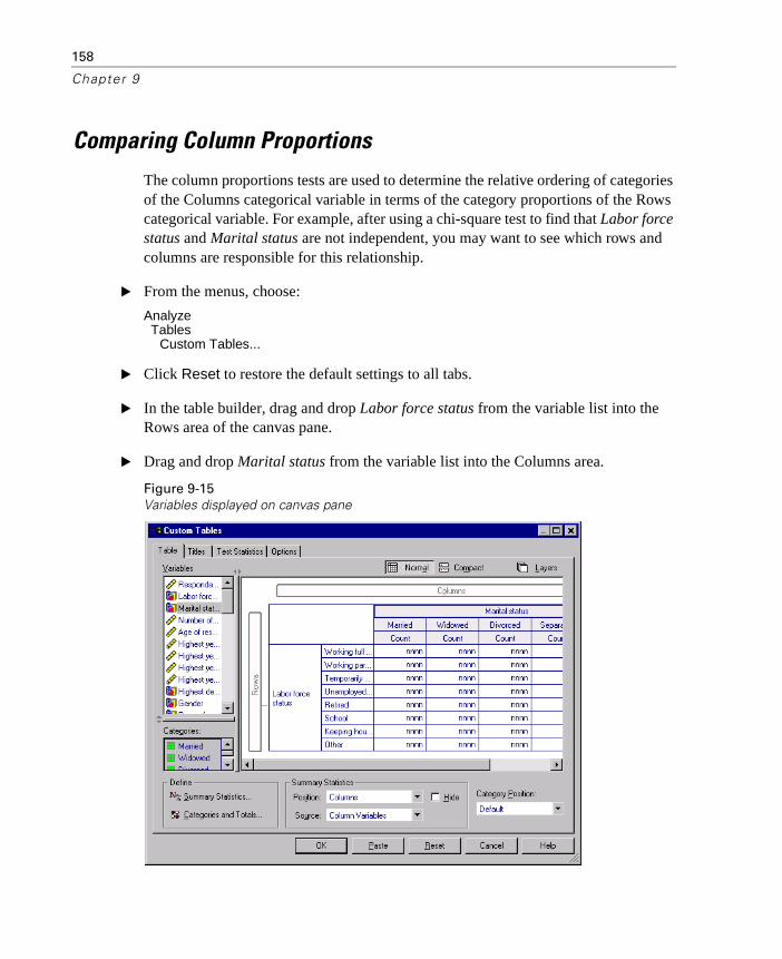
158
Chapter 9
Comparing Column Proportions
The column proportions tests are used to determine the relative ordering of categories of the Columns categorical variable in terms of the category proportions of the Rows categorical variable. For example, after using a chi-square test to find that Labor force status and Marital status are not independent, you may want to see which rows and columns are responsible for this relationship.
� From the menus, choose:
AnalyzeTables
Custom Tables...
� Click Reset to restore the default settings to all tabs.
� In the table builder, drag and drop Labor force status from the variable list into the Rows area of the canvas pane.
� Drag and drop Marital status from the variable list into the Columns area.
Figure 9-15Variables displayed on canvas pane
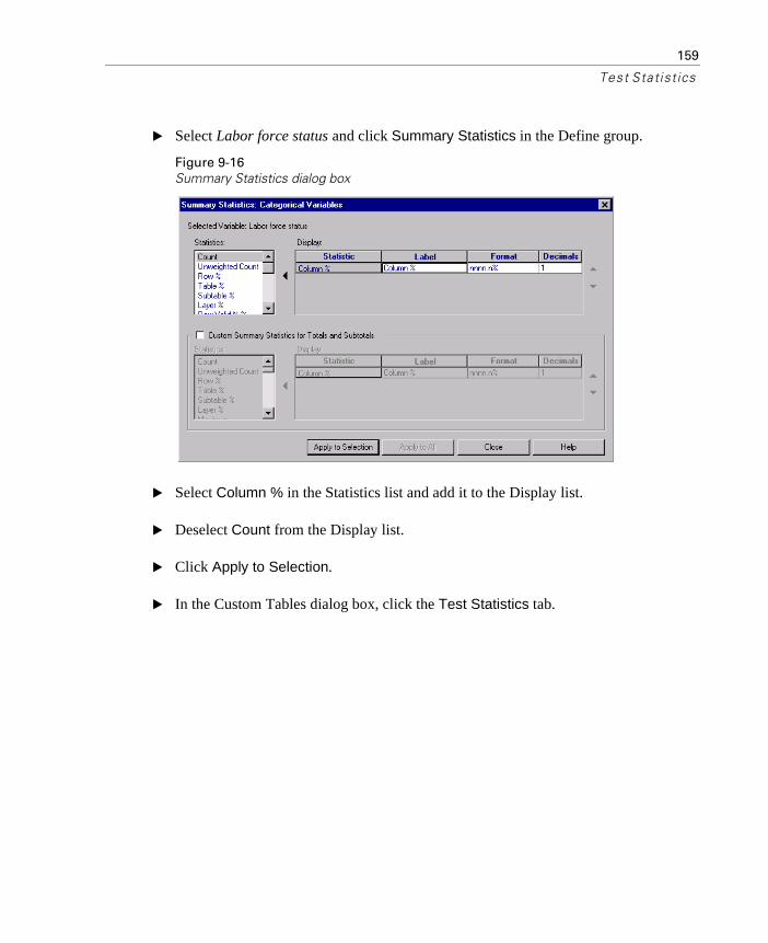
159
Test Statist ics
� Select Labor force status and click Summary Statistics in the Define group.
Figure 9-16Summary Statistics dialog box
� Select Column % in the Statistics list and add it to the Display list.
� Deselect Count from the Display list.
� Click Apply to Selection.
� In the Custom Tables dialog box, click the Test Statistics tab.
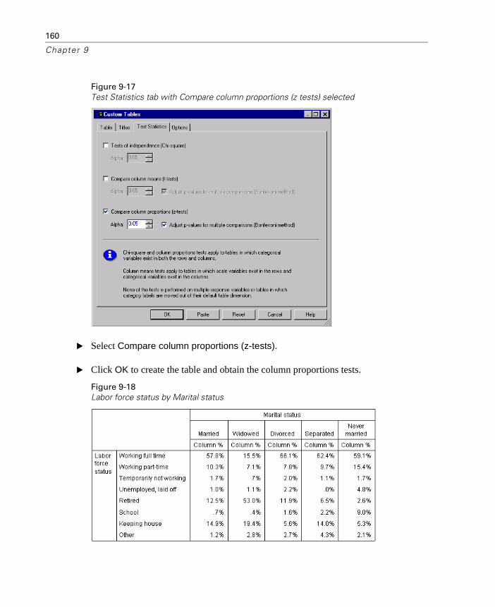
160
Chapter 9
Figure 9-17Test Statistics tab with Compare column proportions (z tests) selected
� Select Compare column proportions (z-tests).
� Click OK to create the table and obtain the column proportions tests.
Figure 9-18Labor force status by Marital status

161
Test Statist ics
This table is a crosstabulation of Labor force status by Marital status, with column proportions shown as the summary statistic.
Figure 9-19Comparisons of column proportions
The column proportions test table assigns a letter key to each category of the column variables. For Marital status, the category Married is assigned the letter A, Widowed is assigned the letter B, and so on, through the category Never married, which is assigned the letter E. For each pair of columns, the column proportions are compared using a z test. Seven sets of column proportions tests are performed, one for each level of Labor force status. Since there are 5 levels of Marital status, 10 pairs of columns ( ) are compared in each set of tests, and Bonferroni adjustments are used to adjust the significance values. For each significant pair, the key of the smaller category is placed under the category with the larger proportion.
For the set of tests associated with Working full time, the B key appears in each of the other columns. Also, the A key appears in C’s column. No other keys are reported in other columns. Thus, you can conclude that the proportion of divorced persons who are working full time is greater than the proportion of married persons working full time, which in turn is greater than the proportion of widowers working full time. The proportions of people who are separated or never married and working full time cannot be differentiated from people who are divorced or married and working full time, but these proportions are greater than the proportion of widowers working full time.
For the tests associated with Working part time or School, the A, B, and C keys appear in E’s column. No other keys are reported in other columns. Thus, the proportions of people who have never been married and are in school or are working
5 4×( ) 2⁄
162
Chapter 9
part time are greater than the proportions of married, widowed, or divorced people who are in school or working part time.
For the tests associated with Temporarily not working or with Other labor status, no other keys are reported in any columns. Thus, there is no discernible difference in the proportions of married, widowed, divorced, separated, or never-married people who are temporarily not working or are in an otherwise uncategorized employment situation.
The tests associated with Retired show that the proportion of widowers who are retired is greater than the proportions of all other marital categories who are retired. Moreover, the proportions of married or divorced people who are retired is greater than the proportion of never-married persons who are retired.
There are greater proportions of people married, widowed, or separated and keeping house than proportions of people divorced or never married and keeping house.
The proportion of people who have never been married and are unemployed, laid off is higher than the proportions of people who are married or widowed and unemployed. Also, note that the Separated column is marked with a “.”, which indicates that the observed proportion of separated people in the Unemployed, laid off row is either 0 or 1, and therefore no comparisons can be made using that column for unemployed respondents.
Effects of Nesting and Stacking on Column Proportions Tests
The rule for column proportions tests is as follows: a separate set of pairwise tests is performed for each innermost subtable. To see how nesting affects the tests, consider the previous example, but with Labor force status nested within levels of Gender.
� Open the table builder again (Analyze menu, Tables, Custom Tables).
� Drag and drop Gender from the variable list into the Rows area of the canvas pane.
� Click OK to create the table.

163
Test Statist ics
Figure 9-20Comparisons of column proportions
With Labor force status nested within levels of Gender, 14 sets of column proportions tests are performed—one for each level of Labor force status for each level of Gender. The same letter keys are assigned to the categories of Marital status.
There are a couple of things to note about the table results:
� With more tests, there are more columns with zero column proportion. They are most common among separated respondents and widowed males.
� The column differences previously seen among respondents keeping house seems to be entirely due to females.
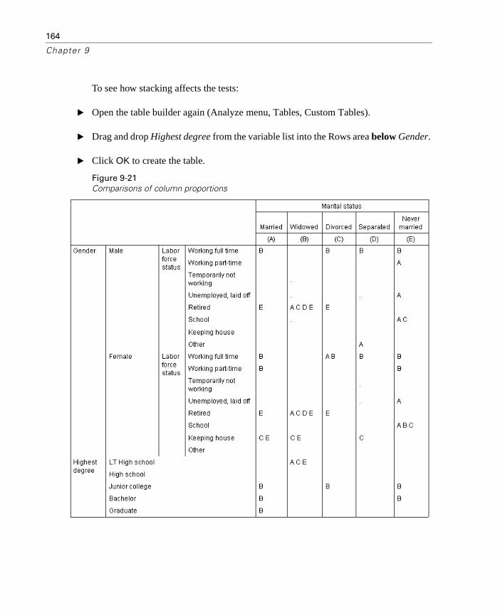
164
Chapter 9
To see how stacking affects the tests:
� Open the table builder again (Analyze menu, Tables, Custom Tables).
� Drag and drop Highest degree from the variable list into the Rows area below Gender.
� Click OK to create the table.
Figure 9-21Comparisons of column proportions
165
Test Statist ics
With Highest degree stacked with Gender, 19 sets of column means tests are performed—the 14 previously discussed plus one for each level of Highest degree. The same letter keys are assigned to the categories of Marital status.
There are a few things to note about the table results:
� The test results for the 14 previously run sets of tests are the same.
� People who have LT high school degree are more common among widowers than among married, divorced, or never-married respondents.
� People with some post-high school education tend to be more common among those people who are married, divorced, and never married than among widowers.

167
Chapte r
10Multiple Response Sets
Custom Tables supports a special kind of “variable” called a multiple response set. Multiple response sets aren’t really “variables” in the normal sense. You can’t see them in the Data Editor, and other procedures don’t recognize them. Multiple response sets use multiple variables to record responses to questions where the respondent can give more than one answer. Multiple response sets are treated like categorical variables, and most of the things you can do with categorical variables you can also do with multiple response sets.
Multiple response sets are constructed from multiple variables in the data file. A multiple response set is a special construct within an SPSS-format data file. You can define and save multiple sets in an SPSS-format data file, but you cannot import or export multiple response sets from/to other file formats. (You can copy multiple response sets from other SPSS data files using Copy Data Properties on the Data menu in the Data Editor window.)
Note: Custom Tables does not support significance testing for tables that contain multiple response sets.
Sample Data File
The examples in this chapter use the data file survey_sample.sav. This file is located in the tutorial\sample_files folder within the folder in which SPSS is installed.
All examples provided here display variable labels in dialog boxes, sorted in alphabetical order. Variable list display properties are set on the General tab in the Options dialog box (Edit menu, Options).

168
Chapter 10
Defining Multiple Response Sets
To define multiple response sets:
� From the menus, choose:
AnalyzeTables
Multiple Response Sets...
Figure 10-1Multiple Response Sets dialog box
� Select two or more variables.
� If your variables are coded as dichotomies, indicate which value you want to have counted.
� Enter a unique name for each multiple response set. The name can be up to seven characters long. A dollar sign is automatically added to the beginning of the set name.
� Enter a descriptive label for the set. (This is optional.)
� Click Add to add the multiple response set to the list of defined sets.

169
Multiple Response Sets
Dichotomies
A multiple dichotomy set typically consists of multiple dichotomous variables: variables with only two possible values of a yes/no, present/absent, checked/not checked nature. Although the variables may not be strictly dichotomous, all of the variables in the set are coded the same way and the Counted Value represents the positive/present/checked condition.
For example, a survey asks the question, “Which of the following sources do you rely on for news?” and provides five possible responses. The respondent can indicate multiple choices by checking a box next to each choice. The five responses become five variables in the data file, coded 0 for No (not checked) and 1 for Yes (checked). In the multiple dichotomy set, the Counted Value is 1.
The sample data file already has three defined multiple response sets. $mltnews is a multiple dichotomy set.
� Select (click) $mltnews in the Mult. Response Sets list.
This displays the variables and settings used to define this multiple response set.
� The Variables in Set list displays the five variables used to construct the multiple response set.
� The Variables Are Coded As group indicates that the variables are dichotomous.
� The Counted Value is 1.
� Select (click) one of the variables in the Variables in Set list.
� Right-click the variable and select Variable Information from the pop-up context menu.
� In the Variable Information window, click the arrow on the Value Labels drop-down list to display the entire list of defined value labels.
Figure 10-2Variable information for multiple dichotomy source variable
170
Chapter 10
The value labels indicate that the variable is a dichotomy with values of 0 and 1, representing No and Yes, respectively. All five variables in the list are coded the same way, and the value of 1 (the code for Yes) is the counted value for the multiple dichotomy set.
Categories
A multiple category set consists of multiple variables, all coded the same way, often with many possible response categories. For example, a survey item states, “Name up to three nationalities that best describe your ethnic heritage.” There may be hundreds of possible responses, but for coding purposes the list is limited to the 40 most common nationalities, with everything else relegated to an “other” category. In the data file, the three choices become three variables, each with 41 categories (40 coded nationalities and one “other” category).
In the sample data file, $ethmult and $mltcars are multiple category sets.
Basic Rules for Multiple Response Sets
� All variables in the set should be coded the same way.
� Value labels should be used consistently. If one variable has defined value labels, all of the variables should have the same value assigned to the same value labels.
� For multiple dichotomy sets, any defined variable labels for variables in the set should be unique. Two or more variables in the set should not have the same variable label.
Counts, Responses, Percentages, and Totals
All of the summary statistics available for categorical variables are also available for multiple response sets. Some additional statistics are also available for multiple response sets.
� From the menus, choose:
Analyze Tables
Custom Tables...
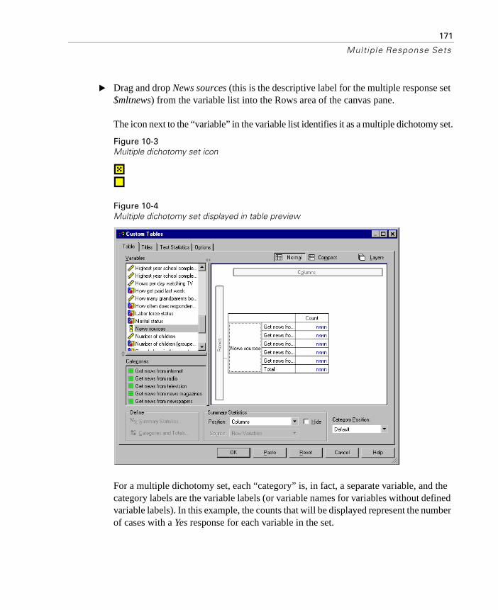
171
Multiple Response Sets
� Drag and drop News sources (this is the descriptive label for the multiple response set $mltnews) from the variable list into the Rows area of the canvas pane.
The icon next to the “variable” in the variable list identifies it as a multiple dichotomy set.
Figure 10-3Multiple dichotomy set icon
Figure 10-4Multiple dichotomy set displayed in table preview
For a multiple dichotomy set, each “category” is, in fact, a separate variable, and the category labels are the variable labels (or variable names for variables without defined variable labels). In this example, the counts that will be displayed represent the number of cases with a Yes response for each variable in the set.

172
Chapter 10
� Right-click News sources in the table preview on the canvas pane and select Categories and Totals from the pop-up context menu.
� Select (click) Total in the Categories and Totals dialog box, and then click Apply.
� Right-click News sources again and select Summary Statistics from the pop-up context menu.
� In the Summary Statistics dialog box, select Column % in the Statistics list and click the arrow to add it to the Display list.
� Click Apply to Selection, and then click OK to create the table.
Figure 10-5Multiple dichotomy counts and column percentages
Totals That Don’t Add Up
If you look at the numbers in the table, you may notice that there is a fairly large discrepancy between the “totals” and the values that are supposedly being totaled—specifically, the totals appear to be much lower than they should be. This is because the count for each “category” in the table is the number of cases with a value of 1 (a Yes response) for that variable, and the total number of Yes responses for all five variables in the multiple dichotomy set might easily exceed the total number of cases in the data file.
The total “count,” however, is the total number of cases with a Yes response for at least one variable in the set, which can never exceed the total number of cases in the data file. In this example, the total count of 2,081 is almost 800 lower than the total number of cases in the data file. If none of these variables have missing values, this means that almost 800 survey respondents indicated that they don’t get news from any of those sources. The total count is the base for the column percentages; so the column percentages in this example sum to more than the 100% displayed for the total column percentage.
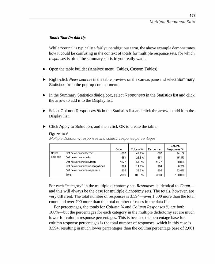
173
Multiple Response Sets
Totals That Do Add Up
While “count” is typically a fairly unambiguous term, the above example demonstrates how it could be confusing in the context of totals for multiple response sets, for which responses is often the summary statistic you really want.
� Open the table builder (Analyze menu, Tables, Custom Tables).
� Right-click News sources in the table preview on the canvas pane and select Summary Statistics from the pop-up context menu.
� In the Summary Statistics dialog box, select Responses in the Statistics list and click the arrow to add it to the Display list.
� Select Column Responses % in the Statistics list and click the arrow to add it to the Display list.
� Click Apply to Selection, and then click OK to create the table.
Figure 10-6Multiple dichotomy responses and column response percentages
For each “category” in the multiple dichotomy set, Responses is identical to Count—and this will always be the case for multiple dichotomy sets. The totals, however, are very different. The total number of responses is 3,594—over 1,500 more than the total count and over 700 more than the total number of cases in the data file.
For percentages, the totals for Column % and Column Responses % are both 100%—but the percentages for each category in the multiple dichotomy set are much lower for column response percentages. This is because the percentage base for column response percentages is the total number of responses, which in this case is 3,594, resulting in much lower percentages than the column percentage base of 2,081.
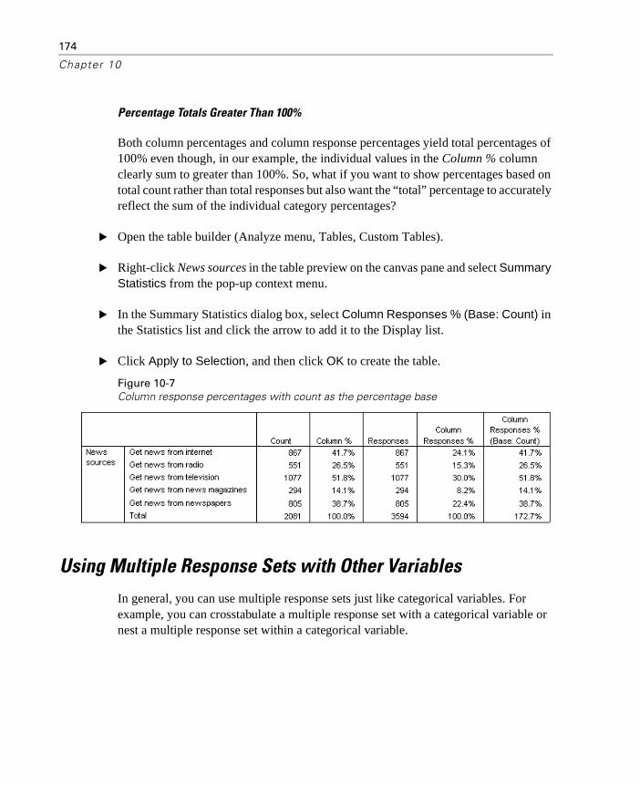
174
Chapter 10
Percentage Totals Greater Than 100%
Both column percentages and column response percentages yield total percentages of 100% even though, in our example, the individual values in the Column % column clearly sum to greater than 100%. So, what if you want to show percentages based on total count rather than total responses but also want the “total” percentage to accurately reflect the sum of the individual category percentages?
� Open the table builder (Analyze menu, Tables, Custom Tables).
� Right-click News sources in the table preview on the canvas pane and select Summary Statistics from the pop-up context menu.
� In the Summary Statistics dialog box, select Column Responses % (Base: Count) in the Statistics list and click the arrow to add it to the Display list.
� Click Apply to Selection, and then click OK to create the table.
Figure 10-7Column response percentages with count as the percentage base
Using Multiple Response Sets with Other Variables
In general, you can use multiple response sets just like categorical variables. For example, you can crosstabulate a multiple response set with a categorical variable or nest a multiple response set within a categorical variable.
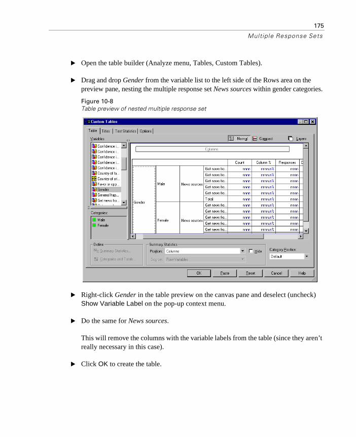
175
Multiple Response Sets
� Open the table builder (Analyze menu, Tables, Custom Tables).
� Drag and drop Gender from the variable list to the left side of the Rows area on the preview pane, nesting the multiple response set News sources within gender categories.
Figure 10-8Table preview of nested multiple response set
� Right-click Gender in the table preview on the canvas pane and deselect (uncheck) Show Variable Label on the pop-up context menu.
� Do the same for News sources.
This will remove the columns with the variable labels from the table (since they aren’t really necessary in this case).
� Click OK to create the table.

176
Chapter 10
Figure 10-9Multiple response set nested within a categorical variable
Statistics Source Variable and Available Summary Statistics
In the absence of a scale variable in a table, categorical variables and multiple response sets are treated the same way regarding the statistics source variable: the innermost nested variable in the statistics source dimension is the statistics source variable. Since there are some summary statistics that can be assigned only to multiple response sets, this means that the multiple response set must be the innermost nested variable in the statistics source dimension if you want any of the special multiple response summary statistics.
� Open the table builder (Analyze menu, Tables, Custom Tables).
� In the table preview on the canvas pane, drag and drop News sources to the left of Gender, changing the nesting order.
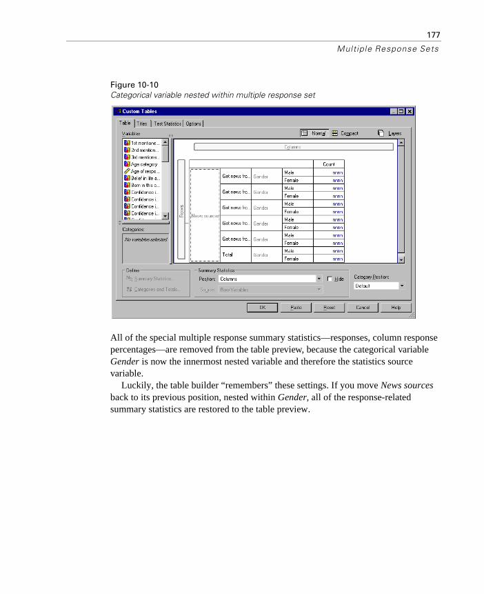
177
Multiple Response Sets
Figure 10-10Categorical variable nested within multiple response set
All of the special multiple response summary statistics—responses, column response percentages—are removed from the table preview, because the categorical variable Gender is now the innermost nested variable and therefore the statistics source variable.
Luckily, the table builder “remembers” these settings. If you move News sources back to its previous position, nested within Gender, all of the response-related summary statistics are restored to the table preview.

178
Chapter 10
Multiple Category Sets and Duplicate Responses
Multiple category sets provide one feature not available for multiple dichotomy sets: the ability to count duplicate responses. In many cases, duplicate responses in multiple category sets probably represent coding errors. For example, for a survey question such as “What three countries do you think make the best cars?” a response of Sweden, Germany, and Sweden probably isn’t valid.
In other cases, however, duplicate responses may be perfectly valid. For example, if the question were “Where were your last three cars made?” a response of Sweden, Germany, and Sweden makes perfect sense.
Custom Tables provides a choice for duplicate responses in multiple category sets. By default, duplicate responses are not counted, but you can request that they be included.
� Open the table builder (Analyze menu, Tables, Custom Tables).
� Click Reset to clear any previous settings.
� Drag and drop Car maker, most recent cars from the variable list into the Rows area of the canvas pane.
The icon next to the “variable” in the variable list identifies it as a multiple category set.
Figure 10-11Multiple category set icon
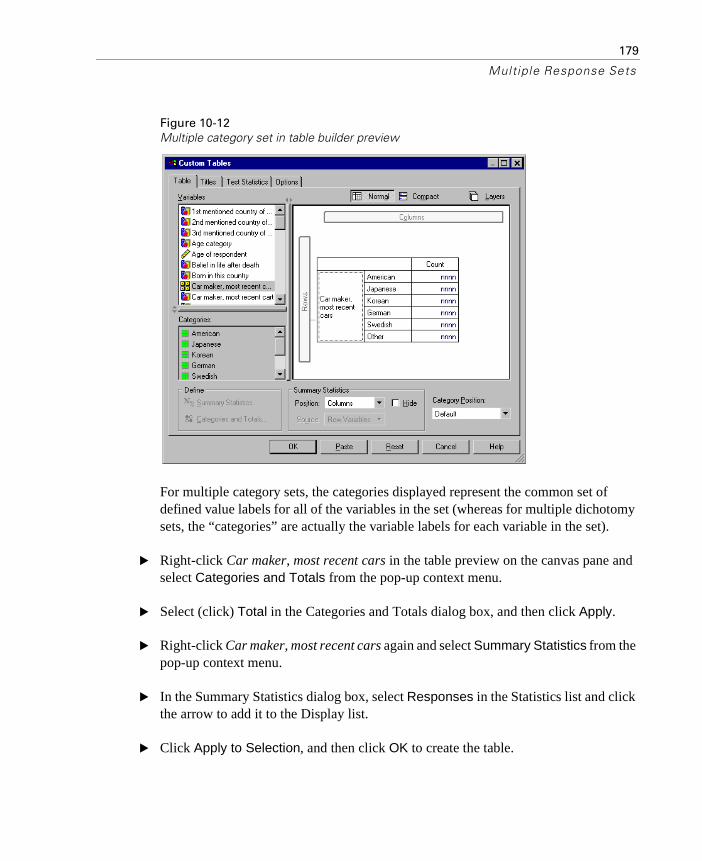
179
Multiple Response Sets
Figure 10-12Multiple category set in table builder preview
For multiple category sets, the categories displayed represent the common set of defined value labels for all of the variables in the set (whereas for multiple dichotomy sets, the “categories” are actually the variable labels for each variable in the set).
� Right-click Car maker, most recent cars in the table preview on the canvas pane and select Categories and Totals from the pop-up context menu.
� Select (click) Total in the Categories and Totals dialog box, and then click Apply.
� Right-click Car maker, most recent cars again and select Summary Statistics from the pop-up context menu.
� In the Summary Statistics dialog box, select Responses in the Statistics list and click the arrow to add it to the Display list.
� Click Apply to Selection, and then click OK to create the table.
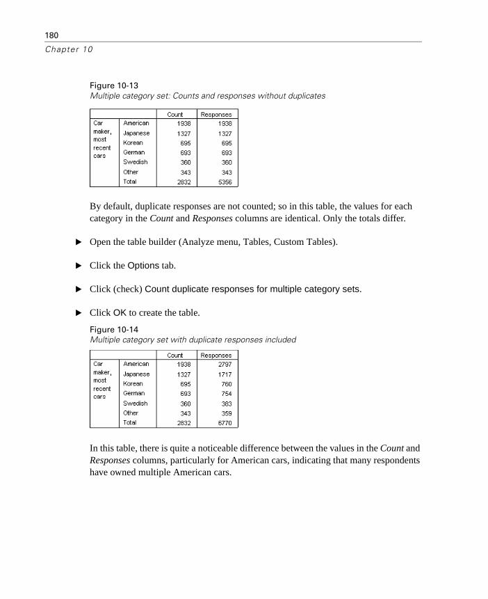
180
Chapter 10
Figure 10-13Multiple category set: Counts and responses without duplicates
By default, duplicate responses are not counted; so in this table, the values for each category in the Count and Responses columns are identical. Only the totals differ.
� Open the table builder (Analyze menu, Tables, Custom Tables).
� Click the Options tab.
� Click (check) Count duplicate responses for multiple category sets.
� Click OK to create the table.
Figure 10-14Multiple category set with duplicate responses included
In this table, there is quite a noticeable difference between the values in the Count and Responses columns, particularly for American cars, indicating that many respondents have owned multiple American cars.

181
Chapte r
11Missing Values
Many data files contain a certain amount of missing data. A wide variety of factors can result in missing data. For example, survey respondents may not answer every question, certain variables may not be applicable to some cases, and coding errors may result in some values being thrown out.
There are two kinds of missing values in SPSS:
� User-missing. Values defined as containing missing data. Value labels can be assigned to these values to identify why the data are missing (such as a code of 99 and a value label of Not Applicable for pregnancy in males).
� System-missing. If no value is present for a numeric variable, it is assigned the system-missing value. This is indicated by a period in the Data View of the Data Editor.
SPSS offers a number of facilities that can help to compensate for the effects of missing data and even analyze patterns in missing data. This chapter, however, has a much simpler goal: to describe how Custom Tables handles missing data and how missing data affect the computation of summary statistics.
Sample Data File
The examples in this chapter use the data file missing_values.sav. This file is located in the tutorial\sample_files folder within the folder in which SPSS is installed. This is a very simple, completely artificial data file, with only one variable and ten cases, designed to illustrate basic concepts about missing values.
182
Chapter 11
Tables without Missing Values
By default, user-missing categories are not displayed in custom tables (and system-missing values are never displayed).
� From the menus, choose:
Analyze Tables
Custom Tables...
� In the table builder, drag and drop Variable with missing values (the only variable in the file) from the variable list into the Rows area of the canvas pane.
� Right-click the variable on the canvas pane and select Categories and Totals from the pop-up context menu.
� Click (check) Total in the Categories and Totals dialog box, and then click Apply.
� Right-click Variable with missing values in the table preview on the canvas pane again and select Summary Statistics from the pop-up context menu.
� In the Summary Statistics dialog box, select Column % in the Statistics list and click the arrow to add it to the Display list.
� Click Apply to Selection.

183
Missing Values
Figure 11-1Table preview without missing values
You may notice a slight discrepancy between the categories displayed in the table preview on the canvas pane and the categories displayed in the Categories list (below the variable list on the left side of the table builder). The Categories list contains a category labeled Missing Values that isn’t included in the table preview because missing value categories are excluded by default. Since “values” is plural in the label, this indicates that the variable has two or more user-missing categories.
� Click OK to create the table.
Figure 11-2Table without missing values
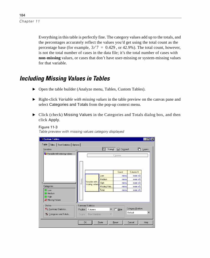
184
Chapter 11
Everything in this table is perfectly fine. The category values add up to the totals, and the percentages accurately reflect the values you’d get using the total count as the percentage base (for example, , or 42.9%). The total count, however, is not the total number of cases in the data file; it’s the total number of cases with non-missing values, or cases that don’t have user-missing or system-missing values for that variable.
Including Missing Values in Tables
� Open the table builder (Analyze menu, Tables, Custom Tables).
� Right-click Variable with missing values in the table preview on the canvas pane and select Categories and Totals from the pop-up context menu.
� Click (check) Missing Values in the Categories and Totals dialog box, and then click Apply.
Figure 11-3Table preview with missing values category displayed
3 7⁄ 0.429=

185
Missing Values
Now the table preview includes a Missing Values category. Although the table preview displays only one category for missing values, all user-missing categories will be displayed in the table.
� Right-click Variable with missing values in the table preview on the canvas pane again and select Summary Statistics from the pop-up context menu.
� In the Summary Statistics dialog box, click (check) Custom Summary Statistics for Totals and Subtotals.
� Select Valid N in the custom summary Statistics list and click the arrow to add it to the Display list.
� Do the same for Total N.
� Click Apply to Selection, and then click OK in the table builder to create the table.
Figure 11-4Table with missing values
The two defined user-missing categories—Don’t know and Not applicable—are now displayed in the table, and the total count is now 9 instead of 7, reflecting the addition of the two cases with user-missing values (one in each user-missing category). The column percentages are also different now, because they are based on the number of non-missing and user-missing values. Only system-missing values are not included in the percentage calculation.
Valid N shows the total number of non-missing cases (7), and Total N shows the total number of cases, including both user-missing and system-missing. The total number of cases is 10, one more than the count of non-missing and user-missing values displayed as the total in the Count column. This is because there’s one case with a system-missing value.

186
Chapter 11
� Open the table builder (Analyze menu, Tables, Custom Tables).
� Right-click Variable with missing values in the table preview on the canvas pane and select Summary Statistics from the pop-up context menu.
� Select Column Valid N% in the top Statistics list (not the custom summaries for totals and subtotals) and click the arrow to add it to the Display list.
� Do the same for Column Total N%.
� You can also add them both to the list of custom summary statistics for totals and subtotals.
� Click Apply to Selection, and then click OK to create the table.
Figure 11-5Table with missing values and valid and total percentages
� Column % is the percentage in each category based on the number of non-missing and user-missing values (since user-missing values have been explicitly included in the table).
� Column Valid N % is the percentage in each category based on only the valid, non-missing cases. These values are the same as the column percentages were in the original table that did not include user-missing values.
� Column Total N % is the percentage in each category based on all cases, including both user-missing and system-missing. If you add up the individual category percentages in this category, you’ll see that they add up to only 90%, because one case out of the total of 10 cases (10%) has the system-missing value. Although this case is included in the base for the percentage calculations, no category is provided in the table for cases with system-missing values.
187
Chapte r
12Formatting and Customizing Tables
Custom Tables provides the ability to control a number of table-formatting properties as part of the table-building process, including:
� Display format and labels for summary statistics
� Minimum and maximum data column width
� Text or value displayed in empty cells
These settings persist within the table builder interface (until you change them, reset the table builder settings, or open a different data file), enabling you to create multiple tables with the same formatting properties without manually editing the tables after creating them. You can also save these formatting settings, along with all of the other table parameters, using the Paste button in the table builder interface to paste command syntax into a syntax window, which you can then save as a file.
You can also change many formatting properties of tables after they have been created, using all of the formatting capabilities available in the Viewer for pivot tables. This chapter, however, focuses on controlling table formatting properties before the table is created. For more information on pivot tables, use the Index tab in the Help system and type pivot tables as the keyword.
Sample Data File
The examples in this chapter use the data file survey_sample.sav. This file is located in the tutorial\sample_files folder within the folder in which SPSS is installed.
All examples provided here display variable labels in dialog boxes, sorted in alphabetical order. Variable list display properties are set on the General tab in the Options dialog box (Edit menu, Options).
188
Chapter 12
Summary Statistics Display Format
Custom Tables attempts to apply relatively intelligent default formats to summary statistics, but there will probably be times when you want to override these defaults.
� From the menus, choose:
Analyze Tables
Custom Tables...
� In the table builder, drag and drop Age category from the variable list into the Rows area on the canvas pane.
� Drag and drop Confidence in television below Age category in the Rows area, stacking the two variables in the row dimension.
� Right-click Age category in the table preview on the canvas pane and select Select All Row Variables from the pop-up context menu.
� Right-click Age category again and select Categories and Totals from the pop-up context menu.
� In the Categories and Totals dialog box, select (check) Total and then click Apply.
� Right-click either variable in the table preview on the canvas pane and select Summary Statistics from the pop-up context menu.
� Select Column % in the Statistics list and click the arrow key to add it to the Display list.
� Select (check) Custom Summary Statistics for Totals and Subtotals.
� In the Statistics list for custom summary statistics, select Column % and click the arrow to add it to the Display list.
� Do the same for Mean.
� Then click Apply to All.
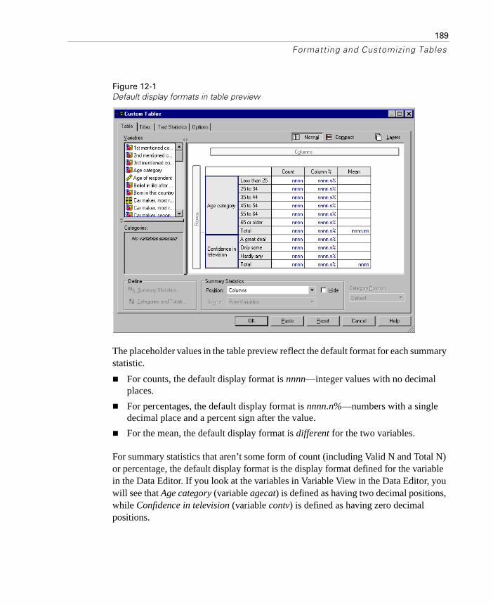
189
Formatt ing and Customizing Tables
Figure 12-1Default display formats in table preview
The placeholder values in the table preview reflect the default format for each summary statistic.
� For counts, the default display format is nnnn—integer values with no decimal places.
� For percentages, the default display format is nnnn.n%—numbers with a single decimal place and a percent sign after the value.
� For the mean, the default display format is different for the two variables.
For summary statistics that aren’t some form of count (including Valid N and Total N) or percentage, the default display format is the display format defined for the variable in the Data Editor. If you look at the variables in Variable View in the Data Editor, you will see that Age category (variable agecat) is defined as having two decimal positions, while Confidence in television (variable contv) is defined as having zero decimal positions.

190
Chapter 12
Figure 12-2Variable View in the Data Editor
This is one of those cases where the default format probably isn’t the format you want, since it would probably be better if both mean values displayed the same number of decimals.
� Right-click either variable in the table preview on the canvas pane and select Summary Statistics from the pop-up context menu.
Figure 12-3Summary Statistics dialog box

191
Formatt ing and Customizing Tables
For the mean, the Format cell in the Display list indicates that the format is Auto, which means that the defined display format for the variable will be used, and the Decimals cell is disabled. In order to specify the number of decimals, you first need to select a different format.
� In the custom summary statistics Display list, click the Format cell for the mean, and select nnnn from the drop-down list of formats.
� In the Decimals cell, enter a value of 1.
� Then click Apply to All to apply this setting to both variables.
Figure 12-4Table preview with user-specified summary statistics display formats
Now the table preview indicates that both mean values will be displayed with one decimal position. (You could go ahead and create this table now—but you might find the “mean” value for Age category a little difficult to interpret, since the actual numeric codes for this variable range only from 1 to 6.)

192
Chapter 12
Display Labels for Summary Statistics
In addition to the display formats for summary statistics, you can also control the descriptive labels for each summary statistic.
� Open the table builder (Analyze menu, Tables, Custom Tables).
� Click Reset to clear any previous settings in the table builder.
� In the table builder, drag and drop Age category from the variable list into the Rows area on the canvas pane.
� Drag and drop How get paid last week from the variable list into the Columns area on the canvas pane.
� Right-click Age category in the table preview on the canvas pane and select Summary Statistics from the pop-up context menu.
� Select Column % in the Statistics list and click the arrow key to add it to the Display list.
� Double-click anywhere in the word Column in the Label cell in the Display list to edit the contents of the cell. Delete the word Column from the label, changing the label to simply %.
� Edit the Label cell for Count in the same way, changing the label to simply N.
While we’re here, let’s change the format of the Column % statistic to remove the unnecessary percent sign (since the column label indicates that the column contains percentages).
� Click the Format cell for Column % and select nnnn.n from the drop-down list of formats.
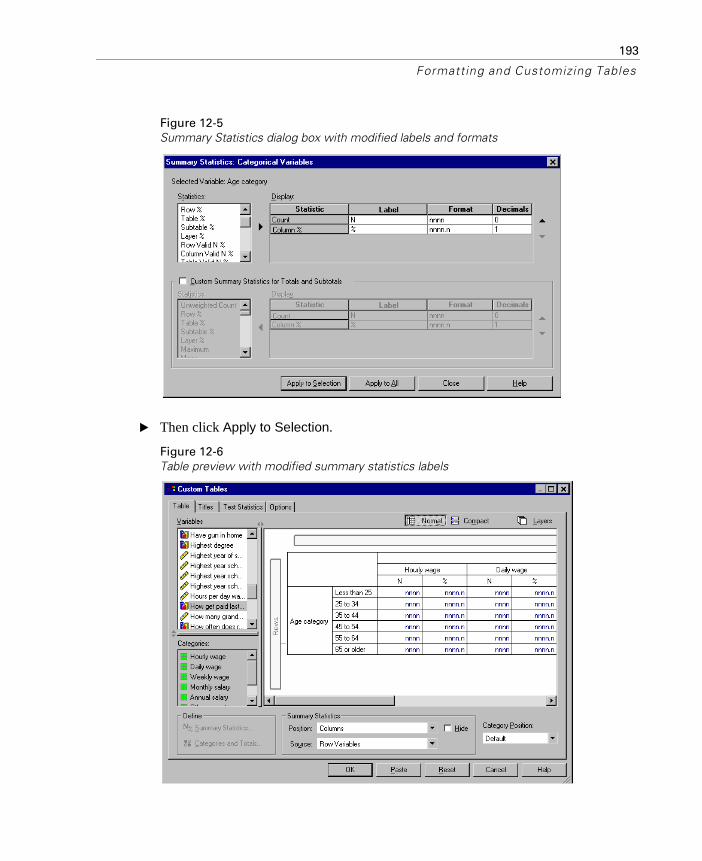
193
Formatt ing and Customizing Tables
Figure 12-5Summary Statistics dialog box with modified labels and formats
� Then click Apply to Selection.
Figure 12-6Table preview with modified summary statistics labels
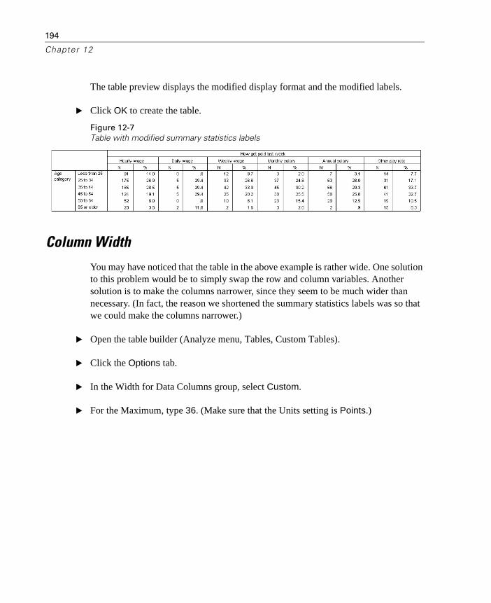
194
Chapter 12
The table preview displays the modified display format and the modified labels.
� Click OK to create the table.
Figure 12-7Table with modified summary statistics labels
Column Width
You may have noticed that the table in the above example is rather wide. One solution to this problem would be to simply swap the row and column variables. Another solution is to make the columns narrower, since they seem to be much wider than necessary. (In fact, the reason we shortened the summary statistics labels was so that we could make the columns narrower.)
� Open the table builder (Analyze menu, Tables, Custom Tables).
� Click the Options tab.
� In the Width for Data Columns group, select Custom.
� For the Maximum, type 36. (Make sure that the Units setting is Points.)

195
Formatt ing and Customizing Tables
Figure 12-8Custom Tables, Options tab
� Click OK to create the table.
Figure 12-9Table with reduced column widths
Now the table is much more compact.
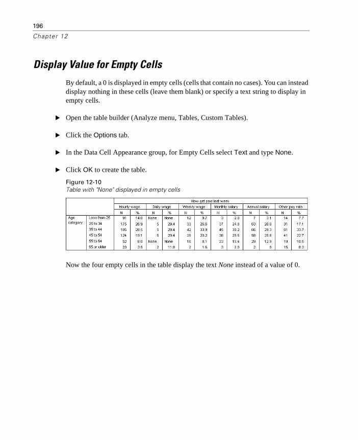
196
Chapter 12
Display Value for Empty Cells
By default, a 0 is displayed in empty cells (cells that contain no cases). You can instead display nothing in these cells (leave them blank) or specify a text string to display in empty cells.
� Open the table builder (Analyze menu, Tables, Custom Tables).
� Click the Options tab.
� In the Data Cell Appearance group, for Empty Cells select Text and type None.
� Click OK to create the table.
Figure 12-10Table with "None" displayed in empty cells
Now the four empty cells in the table display the text None instead of a value of 0.
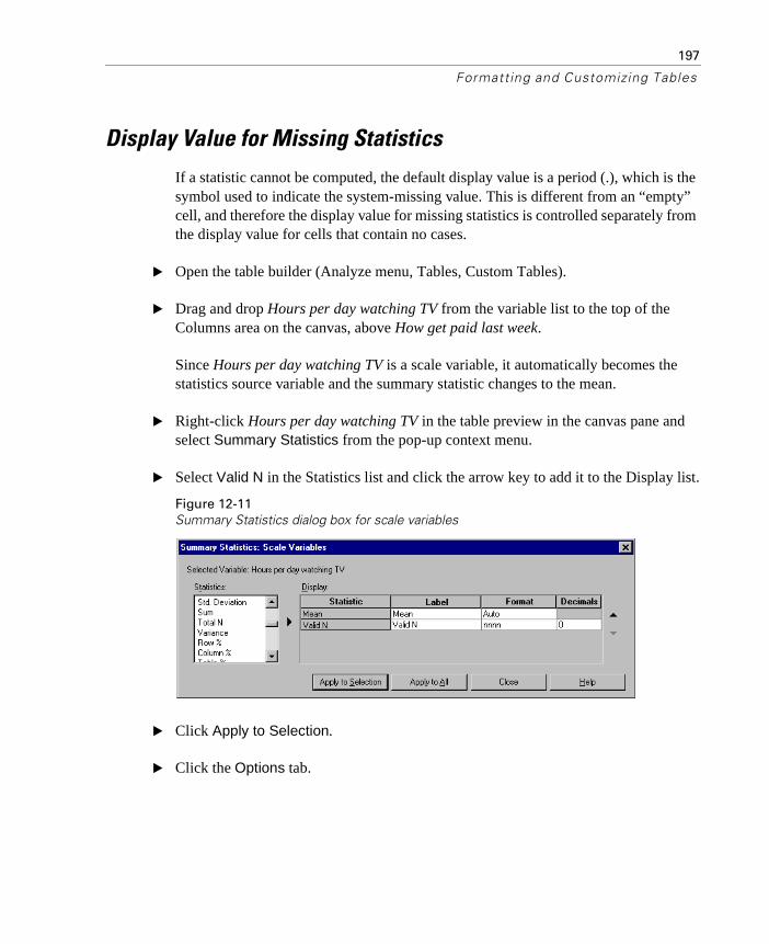
197
Formatt ing and Customizing Tables
Display Value for Missing Statistics
If a statistic cannot be computed, the default display value is a period (.), which is the symbol used to indicate the system-missing value. This is different from an “empty” cell, and therefore the display value for missing statistics is controlled separately from the display value for cells that contain no cases.
� Open the table builder (Analyze menu, Tables, Custom Tables).
� Drag and drop Hours per day watching TV from the variable list to the top of the Columns area on the canvas, above How get paid last week.
Since Hours per day watching TV is a scale variable, it automatically becomes the statistics source variable and the summary statistic changes to the mean.
� Right-click Hours per day watching TV in the table preview in the canvas pane and select Summary Statistics from the pop-up context menu.
� Select Valid N in the Statistics list and click the arrow key to add it to the Display list.
Figure 12-11Summary Statistics dialog box for scale variables
� Click Apply to Selection.
� Click the Options tab.
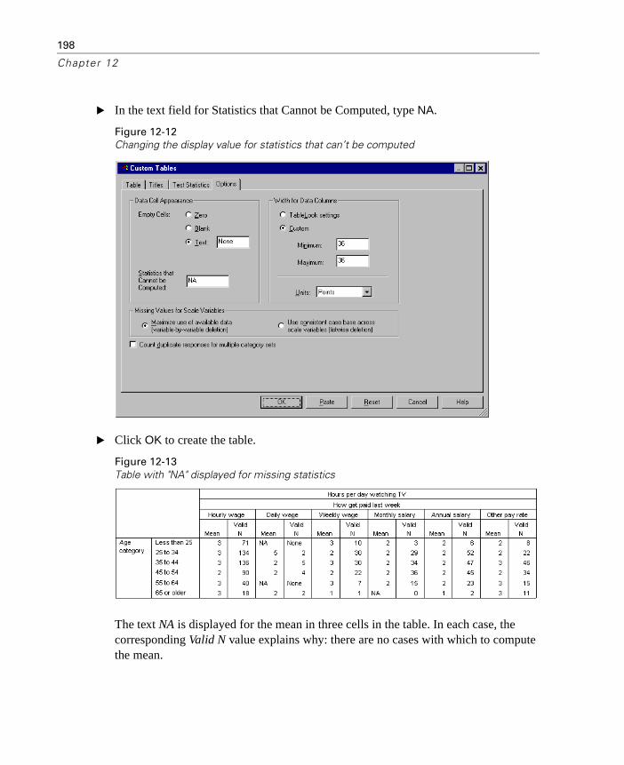
198
Chapter 12
� In the text field for Statistics that Cannot be Computed, type NA.
Figure 12-12Changing the display value for statistics that can’t be computed
� Click OK to create the table.
Figure 12-13Table with "NA" displayed for missing statistics
The text NA is displayed for the mean in three cells in the table. In each case, the corresponding Valid N value explains why: there are no cases with which to compute the mean.

199
Formatt ing and Customizing Tables
You may, however, notice what appears to be slight discrepancy—one of those three Valid N values is displayed as a 0, not the label None that is supposed to be displayed in cells with no cases. This is because although there are no valid cases to use to compute the mean, the category isn’t really empty. If you go back to the original table with just the two categorical variables, you will see that there are, in fact, three cases in this crosstabulated category. There are no valid cases, however, because all three have missing values for the scale variable Hours per day watching TV.
Changing the Default TableLook
Many of the display properties of pivot tables can be controlled with TableLooks. A wide variety of predefined TableLooks are available, and you can control the default TableLook that determines the display properties applied to pivot tables when they are created.
� From the menus, choose:
Edit Options...
� Click the Pivot Tables tab.
� From the list of TableLooks, select Contrast 3.tlo.
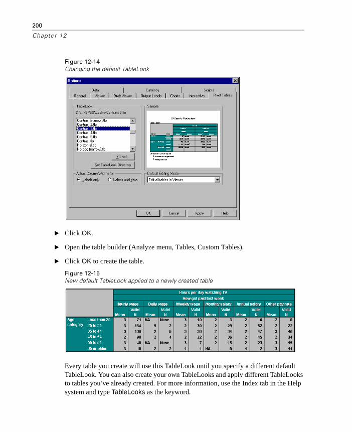
200
Chapter 12
Figure 12-14Changing the default TableLook
� Click OK.
� Open the table builder (Analyze menu, Tables, Custom Tables).
� Click OK to create the table.
Figure 12-15New default TableLook applied to a newly created table
Every table you create will use this TableLook until you specify a different default TableLook. You can also create your own TableLooks and apply different TableLooks to tables you’ve already created. For more information, use the Index tab in the Help system and type TableLooks as the keyword.

Syntax Reference

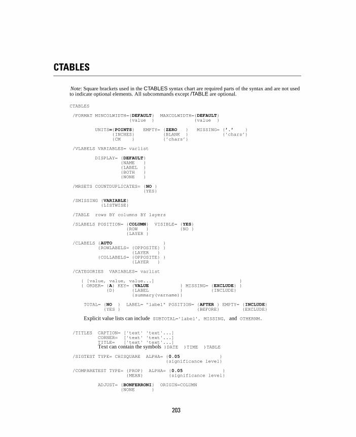
203
CTABLES
Note: Square brackets used in the CTABLES syntax chart are required parts of the syntax and are not used to indicate optional elements. All subcommands except /TABLE are optional.
CTABLES
/FORMAT MINCOLWIDTH={DEFAULT} MAXCOLWIDTH={DEFAULT} {value } {value }
UNITS={POINTS} EMPTY= {ZERO } MISSING= {’.’ } {INCHES} {BLANK } {’chars’} {CM } {’chars’}
/VLABELS VARIABLES= varlist
DISPLAY= {DEFAULT} {NAME } {LABEL } {BOTH } {NONE }
/MRSETS COUNTDUPLICATES= {NO } {YES}
/SMISSING {VARIABLE} {LISTWISE}
/TABLE rows BY columns BY layers
/SLABELS POSITION= {COLUMN} VISIBLE= {YES} {ROW } {NO } {LAYER }
/CLABELS {AUTO } {ROWLABELS= {OPPOSITE} } {LAYER } {COLLABELS= {OPPOSITE} } {LAYER }
/CATEGORIES VARIABLES= varlist
{ [value, value, value...] } { ORDER= {A} KEY= {VALUE } MISSING= {EXCLUDE} } {D} {LABEL } {INCLUDE} {summary(varname)}
TOTAL= {NO } LABEL= "label" POSITION= {AFTER } EMPTY= {INCLUDE} {YES } {BEFORE} {EXCLUDE}
Explicit value lists can include SUBTOTAL=’label’, MISSING, and OTHERNM.
/TITLES CAPTION= ['text' 'text'...] CORNER= ['text' 'text'...] TITLE= ['text' 'text'...] Text can contain the symbols )DATE )TIME )TABLE
/SIGTEST TYPE= CHISQUARE ALPHA= {0.05 } {significance level}
/COMPARETEST TYPE= {PROP} ALPHA= {0.05 } {MEAN} {significance level}
ADJUST= {BONFERRONI} ORIGIN=COLUMN {NONE }

204 CTABLES
Row, column, and layer elements each have the general form
varname {[C]} [summary ‘label’ format...] {+} varname ... {[S]} {>}
When nesting (>) and concatenation (+) are combined, as in a + b > c, nesting occurs before concatenation; parentheses can be used to change precedence, as in (a + b) > c.
Summary functions available for all variables: COUNT ROWPCT.COUNT COLPCT.COUNT TABLEPCT.COUNT SUBTABLEPCT.COUNT LAYERPCT.COUNT LAYERROWPCT.COUNT LAYERCOLPCT.COUNT ROWPCT.VALIDN COLPCT.VALIDN TABLEPCT.VALIDN SUBTABLEPCT.VALIDN LAYERPCT.VALIDN LAYERROWPCT.VALIDN LAYERCOLPCT.VALIDN ROWPCT.TOTALN COLPCT.TOTALN TABLEPCT.TOTALN SUBTABLEPCT.TOTALN LAYERPCT.TOTALN LAYERROWPCT.TOTALN LAYERCOLPCT.TOTALN
Summary functions available for scale variables and for totals, and subtotals of numeric variables: MAXIMUM MEAN MEDIAN MINIMUM MISSING MODE PTILE RANGE SEMEAN STDDEV SUM TOTALN VALIDN VARIANCE ROWPCT.SUM COLPCT.SUM TABLEPCT.SUM SUBTABLEPCT.SUM LAYERPCT.SUM LAYERROWPCT.SUM LAYERCOLPCT.SUM
Summary functions available for multiple response variables and their totals: RESPONSES ROWPCT.RESPONSES COLPCT.RESPONSES TABLEPCT.RESPONSES SUBTABLEPCT.RESPONSES LAYERPCT.RESPONSES LAYERROWPCT.RESPONSES LAYERCOLPCT.RESPONSES ROWPCT.RESPONSES.COUNT COLPCT.RESPONSES.COUNT TABLEPCT.RESPONSES.COUNT SUBTABLEPCT.RESPONSES.COUNT LAYERPCT.RESPONSES.COUNT LAYERROWPCT.RESPONSES.COUNT LAYERCOLPCT.RESPONSES.COUNT ROWPCT.COUNT.RESPONSES COLPCT.COUNT.RESPONSES TABLEPCT.COUNT.RESPONSES SUBTABLEPCT.COUNT.RESPONSES LAYERPCT.COUNT.RESPONSES LAYERROWPCT. COUNT.RESPONSES LAYERCOLPCT.COUNT.RESPONSES
For unweighted summaries, prefix U to a function name, as in UCOUNT.
Formats for summaries: COMMAw.d DOLLARw.d Fw.d NEGPARENw.d NEQUALw.d PARENw.d PCTw.d PCTPARENw.d DOTw.d CCA...CCEw.d Nw.d Ew.d and all DATE formats
ExamplesCTABLES /TABLE POLVIEWS [COLPCT] BY AGECAT.
CTABLES /TABLE $MLTNEWS [COUNT COLPCT] BY SEX /SLABELS VISIBLE=NO /CATEGORIES VARIABLES=SEX TOTAL=YES.
CTABLES /TABLE (CONFINAN + CONBUS + CONBUS + CONEDUC + CONPRESS + CONMEDIC)[COUNT ROWPCT] /CLABELS ROWLABELS=OPPOSITE.
Overview
The Custom Tables procedure produces tables in one, two, or three dimensions and providesa great deal of flexibility for organizing and displaying the contents.
• In each dimension (row, column, and layer), you can stack multiple variables to concatenatetables and nest variables to create subtables. See the TABLE subcommand.
• You can let Custom Tables determine summary statistics according to the measurementlevel in the dictionary, or you can assign one or more summaries to specific variables andoverride the measurement level without altering the dictionary. See the TABLE subcommand.

CTABLES 205
• You can create multiple response sets with the MRSETS command and use them likeordinary categorical variables in a table expression. You can control the percentage baseby choosing an appropriate summary function, and you can control with the MRSETS sub-command whether duplicate responses from a single respondent are counted.
• You can assign totals to categorical variables at different nesting levels to create subtableand table totals, and you can assign subtotals across subsets of the values of a variable.See the CATEGORIES subcommand.
• You can determine on a per-variable basis which categories to display in the table, includ-ing whether to display missing values and empty categories for which variable labels exist.You can also sort categories by name, label, or the value of a summary function. See theCATEGORIES subcommand.
• You can specify whether to show or hide summary and category labels and where toposition the labels. For variable labels, you can specify whether to show labels, names,both, or neither. See the SLABELS, CLABELS, and VLABELS subcommands.
• You can request chi-square tests and pairwise comparisons of column proportions andmeans. See the SIGTEST and COMPARETEST subcommands.
• You can assign custom titles and captions (see the TITLES subcommand) and control whatdisplays for empty cells and those for which a summary function cannot be computed. Seethe FORMAT subcommand.
• CTABLES ignores SPLIT FILE requests if layered splits (compare groups in the graphicaluser interface) are requested. You can compare groups by using the split variables at thehighest nesting level for row variables. See the TABLE subcommand for nesting variables.
Syntax Conventions
• The basic specification is a TABLE subcommand with at least one variable in onedimension. Multiple TABLE subcommands can be included in one CTABLES command.
• The global subcommands FORMAT, VLABELS, MRSETS, and SMISSING must precede thefirst TABLE subcommand and can be named in any order.
• The local subcommands SLABELS, CLABELS, CATEGORIES, TITLES, SIGTEST, andCOMPARETEST follow the TABLE subcommand in any order and refer to the immediatelypreceding table expression.
• In general, if subcommands are repeated, their specifications are merged. The last valueof each specified attribute is honored.
• Equals signs shown in the syntax charts are required.
• Square brackets shown in the syntax charts are required.
• All keywords except summary function names, attribute values, and explicit category listkeywords can be truncated to as few as three characters. Function names must be spelledin full.
• The slash before all subcommands, including the first, is required.
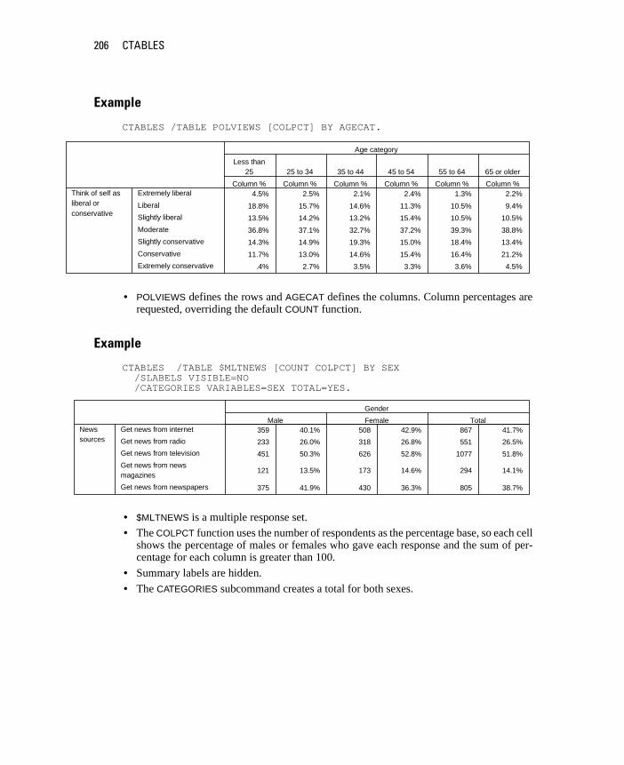
206 CTABLES
Example
CTABLES /TABLE POLVIEWS [COLPCT] BY AGECAT.
• POLVIEWS defines the rows and AGECAT defines the columns. Column percentages arerequested, overriding the default COUNT function.
Example
CTABLES /TABLE $MLTNEWS [COUNT COLPCT] BY SEX /SLABELS VISIBLE=NO /CATEGORIES VARIABLES=SEX TOTAL=YES.
• $MLTNEWS is a multiple response set. • The COLPCT function uses the number of respondents as the percentage base, so each cell
shows the percentage of males or females who gave each response and the sum of per-centage for each column is greater than 100.
• Summary labels are hidden.
• The CATEGORIES subcommand creates a total for both sexes.
4.5% 2.5% 2.1% 2.4% 1.3% 2.2%
18.8% 15.7% 14.6% 11.3% 10.5% 9.4%
13.5% 14.2% 13.2% 15.4% 10.5% 10.5%
36.8% 37.1% 32.7% 37.2% 39.3% 38.8%
14.3% 14.9% 19.3% 15.0% 18.4% 13.4%
11.7% 13.0% 14.6% 15.4% 16.4% 21.2%
.4% 2.7% 3.5% 3.3% 3.6% 4.5%
Extremely liberal
Liberal
Slightly liberal
Moderate
Slightly conservative
Conservative
Extremely conservative
Think of self asliberal orconservative
Column %
Less than25
Column %
25 to 34
Column %
35 to 44
Column %
45 to 54
Column %
55 to 64
Column %
65 or older
Age category
359 40.1% 508 42.9% 867 41.7%
233 26.0% 318 26.8% 551 26.5%
451 50.3% 626 52.8% 1077 51.8%
121 13.5% 173 14.6% 294 14.1%
375 41.9% 430 36.3% 805 38.7%
Get news from internet
Get news from radio
Get news from television
Get news from newsmagazines
Get news from newspapers
Newssources
Male Female Total
Gender

CTABLES 207
Example
CTABLES /TABLE (CONFINAN + CONBUS + CONBUS + CONEDUC + CONPRESS + CONMEDIC)[COUNT ROWPCT] /CLABELS ROWLABELS=OPPOSITE.
• The six confidence variables all have the same categories with the same value labels foreach.
• The CLABELS subcommand moves the category labels to the columns.
TABLE Subcommand
The TABLE subcommand specifies the structure of the table, including the variables and sum-mary functions that define each dimension. It has the general form
/TABLE rows BY columns BY layers
The minimum specification for a row, column, or layer is a variable name. You can specifyone or more dimensions.
Variable Types
The variables used in a table expression can be category variables, scale variables, or multipleresponse sets. Multiple response sets are defined by the MRSETS command in the SPSS Baseand always begin with a $. Custom Tables uses the measurement level in the dictionary forthe active data file to identify category and scale variables. You can override the default vari-able type for numeric variables by placing [C] or [S] after the variable name. Thus, to treat thecategory variable HAPPY as a scale variable and obtain a mean, you would specify
/TABLE HAPPY [S].
Category Variables and Multiple Response Sets
Category variables define one cell per value. See the CATEGORIES subcommand for waysof controlling how categories are displayed. Multiple response sets also define one cellper value.
490 26.3% 1068 57.3% 306 16.4%
500 27.5% 1078 59.2% 243 13.3%
500 27.5% 1078 59.2% 243 13.3%
511 27.2% 1055 56.1% 315 16.7%
176 9.5% 878 47.2% 808 43.4%
844 45.0% 864 46.1% 167 8.9%
Confidence in banks &financial institutions
Confidence in majorcompanies
Confidence in majorcompanies
Confidence in education
Confidence in press
Confidence in medicine
Count Row %
A great deal
Count Row %
Only some
Count Row %
Hardly any
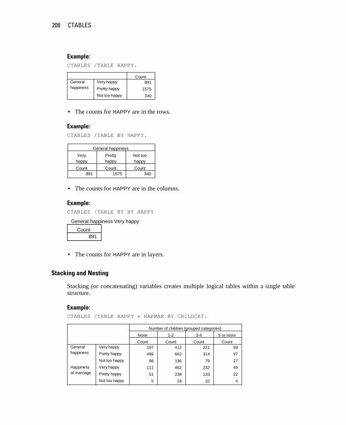
208 CTABLES
Example:CTABLES /TABLE HAPPY.
• The counts for HAPPY are in the rows.
Example:CTABLES /TABLE BY HAPPY.
• The counts for HAPPY are in the columns.
Example:CTABLES /TABLE BY BY HAPPY
• The counts for HAPPY are in layers.
Stacking and Nesting
Stacking (or concatenating) variables creates multiple logical tables within a single tablestructure.
Example:CTABLES /TABLE HAPPY + HAPMAR BY CHILDCAT.
891
1575
340
Very happy
Pretty happy
Not too happy
Generalhappiness
Count
891 1575 340Count
Veryhappy
Count
Prettyhappy
Count
Not toohappy
General happiness
General happiness Very happy
891Count
197 412 221 59
499 662 314 97
98 136 79 27
111 462 232 49
51 238 133 22
5 18 10 4
Very happy
Pretty happy
Not too happy
Generalhappiness
Very happy
Pretty happy
Not too happy
Happinessof marriage
Count
None
Count
1-2
Count
3-4
Count
5 or more
Number of children (grouped categories)
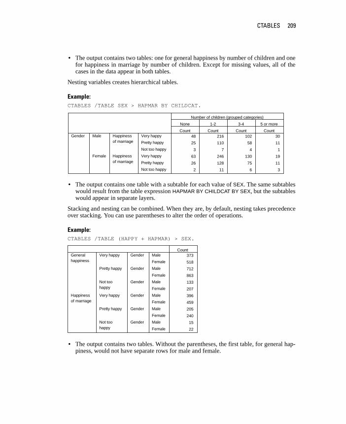
CTABLES 209
• The output contains two tables: one for general happiness by number of children and onefor happiness in marriage by number of children. Except for missing values, all of thecases in the data appear in both tables.
Nesting variables creates hierarchical tables.
Example:CTABLES /TABLE SEX > HAPMAR BY CHILDCAT.
• The output contains one table with a subtable for each value of SEX. The same subtableswould result from the table expression HAPMAR BY CHILDCAT BY SEX, but the subtableswould appear in separate layers.
Stacking and nesting can be combined. When they are, by default, nesting takes precedenceover stacking. You can use parentheses to alter the order of operations.
Example:CTABLES /TABLE (HAPPY + HAPMAR) > SEX.
• The output contains two tables. Without the parentheses, the first table, for general hap-piness, would not have separate rows for male and female.
48 216 102 30
25 110 58 11
3 7 4 1
63 246 130 19
26 128 75 11
2 11 6 3
Very happy
Pretty happy
Not too happy
Happinessof marriage
Male
Very happy
Pretty happy
Not too happy
Happinessof marriage
Female
GenderCount
None
Count
1-2
Count
3-4
Count
5 or more
Number of children (grouped categories)
373
518
712
863
133
207
396
459
205
240
15
22
Male
Female
GenderVery happy
Male
Female
GenderPretty happy
Male
Female
GenderNot toohappy
Generalhappiness
Male
Female
GenderVery happy
Male
Female
GenderPretty happy
Male
Female
GenderNot toohappy
Happinessof marriage
Count
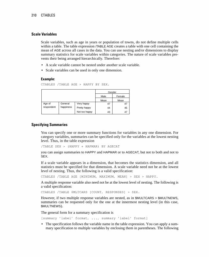
210 CTABLES
Scale Variables
Scale variables, such as age in years or population of towns, do not define multiple cellswithin a table. The table expression /TABLE AGE creates a table with one cell containing themean of AGE across all cases in the data. You can use nesting and/or dimensions to displaysummary statistics for scale variables within categories. The nature of scale variables pre-vents their being arranged hierarchically. Therefore:
• A scale variable cannot be nested under another scale variable.
• Scale variables can be used in only one dimension.
Example:CTABLES /TABLE AGE > HAPPY BY SEX.
Specifying Summaries
You can specify one or more summary functions for variables in any one dimension. Forcategory variables, summaries can be specified only for the variables at the lowest nestinglevel. Thus, in the table expression
/TABLE SEX > (HAPPY + HAPMAR) BY AGECAT
you can assign summaries to HAPPY and HAPMAR or to AGECAT, but not to both and not toSEX.
If a scale variable appears in a dimension, that becomes the statistics dimension, and allstatistics must be specified for that dimension. A scale variable need not be at the lowestlevel of nesting. Thus, the following is a valid specification:
CTABLES /TABLE AGE [MINIMUM, MAXIMUM, MEAN] > SEX > HAPPY.
A multiple response variable also need not be at the lowest level of nesting. The following isa valid specification:
CTABLES /TABLE $MLTCARS [COUNT, RESPONSES] > SEX.
However, if two multiple response variables are nested, as in $MULTCARS > $MULTNEWS,summaries can be requested only for the one at the innermost nesting level (in this case,$MULTNEWS).
The general form for a summary specification is
[summary ’label’ format, ..., summary ’label’ format]
• The specification follows the variable name in the table expression. You can apply a sum-mary specification to multiple variables by enclosing them in parentheses. The following
47 47
44 45
43 47
Very happy
Pretty happy
Not too happy
Generalhappiness
Age ofrespondent
Mean
Male
Mean
Female
Gender
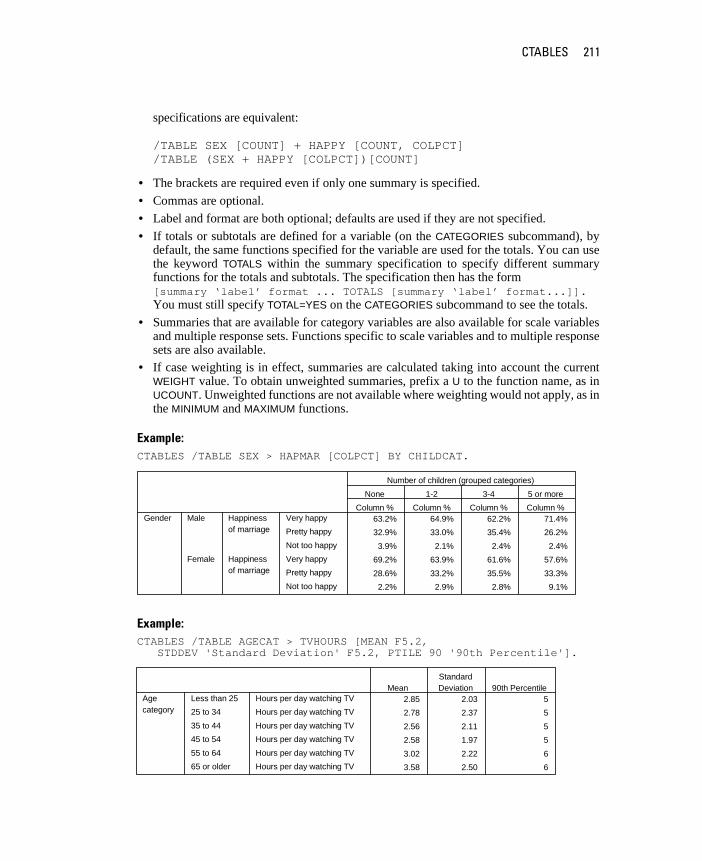
CTABLES 211
specifications are equivalent:
/TABLE SEX [COUNT] + HAPPY [COUNT, COLPCT] /TABLE (SEX + HAPPY [COLPCT])[COUNT]
• The brackets are required even if only one summary is specified.
• Commas are optional.
• Label and format are both optional; defaults are used if they are not specified.
• If totals or subtotals are defined for a variable (on the CATEGORIES subcommand), bydefault, the same functions specified for the variable are used for the totals. You can usethe keyword TOTALS within the summary specification to specify different summaryfunctions for the totals and subtotals. The specification then has the form[summary ‘label’ format ... TOTALS [summary ‘label’ format...]]. You must still specify TOTAL=YES on the CATEGORIES subcommand to see the totals.
• Summaries that are available for category variables are also available for scale variablesand multiple response sets. Functions specific to scale variables and to multiple responsesets are also available.
• If case weighting is in effect, summaries are calculated taking into account the currentWEIGHT value. To obtain unweighted summaries, prefix a U to the function name, as inUCOUNT. Unweighted functions are not available where weighting would not apply, as inthe MINIMUM and MAXIMUM functions.
Example:CTABLES /TABLE SEX > HAPMAR [COLPCT] BY CHILDCAT.
Example:CTABLES /TABLE AGECAT > TVHOURS [MEAN F5.2, STDDEV 'Standard Deviation' F5.2, PTILE 90 '90th Percentile'].
63.2% 64.9% 62.2% 71.4%
32.9% 33.0% 35.4% 26.2%
3.9% 2.1% 2.4% 2.4%
69.2% 63.9% 61.6% 57.6%
28.6% 33.2% 35.5% 33.3%
2.2% 2.9% 2.8% 9.1%
Very happy
Pretty happy
Not too happy
Happinessof marriage
Male
Very happy
Pretty happy
Not too happy
Happinessof marriage
Female
GenderColumn %
None
Column %
1-2
Column %
3-4
Column %
5 or more
Number of children (grouped categories)
2.85 2.03 5
2.78 2.37 5
2.56 2.11 5
2.58 1.97 5
3.02 2.22 6
3.58 2.50 6
Hours per day watching TVLess than 25
Hours per day watching TV25 to 34
Hours per day watching TV35 to 44
Hours per day watching TV45 to 54
Hours per day watching TV55 to 64
Hours per day watching TV65 or older
Agecategory
MeanStandardDeviation 90th Percentile
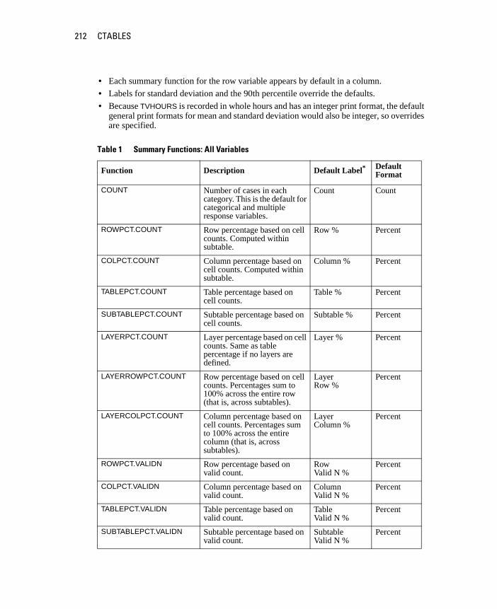
212 CTABLES
• Each summary function for the row variable appears by default in a column.
• Labels for standard deviation and the 90th percentile override the defaults.
• Because TVHOURS is recorded in whole hours and has an integer print format, the defaultgeneral print formats for mean and standard deviation would also be integer, so overridesare specified.
Table 1 Summary Functions: All Variables
Function Description Default Label* Default Format
COUNT Number of cases in each category. This is the default for categorical and multiple response variables.
Count Count
ROWPCT.COUNT Row percentage based on cell counts. Computed within subtable.
Row % Percent
COLPCT.COUNT Column percentage based on cell counts. Computed within subtable.
Column % Percent
TABLEPCT.COUNT Table percentage based on cell counts.
Table % Percent
SUBTABLEPCT.COUNT Subtable percentage based on cell counts.
Subtable % Percent
LAYERPCT.COUNT Layer percentage based on cell counts. Same as table percentage if no layers are defined.
Layer % Percent
LAYERROWPCT.COUNT Row percentage based on cell counts. Percentages sum to 100% across the entire row (that is, across subtables).
LayerRow %
Percent
LAYERCOLPCT.COUNT Column percentage based on cell counts. Percentages sum to 100% across the entire column (that is, across subtables).
LayerColumn %
Percent
ROWPCT.VALIDN Row percentage based on valid count.
Row Valid N %
Percent
COLPCT.VALIDN Column percentage based on valid count.
ColumnValid N %
Percent
TABLEPCT.VALIDN Table percentage based on valid count.
Table Valid N %
Percent
SUBTABLEPCT.VALIDN Subtable percentage based on valid count.
SubtableValid N %
Percent

CTABLES 213
The .COUNT suffix can be omitted from percentages based on cell counts. Thus, ROWPCT isequivalent to ROWPCT.COUNT.
Function Description Default Label Default Format
LAYERPCT.VALIDN Layer percentage based on valid count.
Layer Valid N %
Percent
LAYERROWPCT. VALIDN Row percentage based on valid count. Percentages sum to 100% across the entire row.
Layer Row Valid N %
Percent
LAYERCOLPCT. VALIDN Column percentage based on valid count. Percentages sum to 100% across the entire column.
LayerColumnValid N %
Percent
ROWPCT.TOTALN Row percentage based on total count, including user- and system-missing values.
Row Total N %
Percent
COLPCT.TOTALN Column percentage based on total count, including user- and system-missing values.
Column Total N %
Percent
TABLEPCT.TOTALN Table percentage based on total count, including user- and system-missing values.
Table Total N %
Percent
SUBTABLEPCT.TOTALN Subtable percentage based on total count, including user- and system-missing values.
SubtableTotal N %
Percent
LAYERPCT.TOTALN Layer percentage based on total count, including user- and system-missing values.
Layer Total N %
Percent
LAYERROWPCT. TOTALN Row percentage based on total count, including user- and system-missing values. Percentages sum to 100% across the entire row.
Layer Row Total N %
Percent
LAYERCOLPCT. TOTALN Column percentage based on total count, including user- and system-missing values. Percentages sum to 100% across the entire column.
Layer Column Total N %
Percent
* This is the default on a U.S.-English system.
Table 1 Summary Functions: All Variables (Continued)
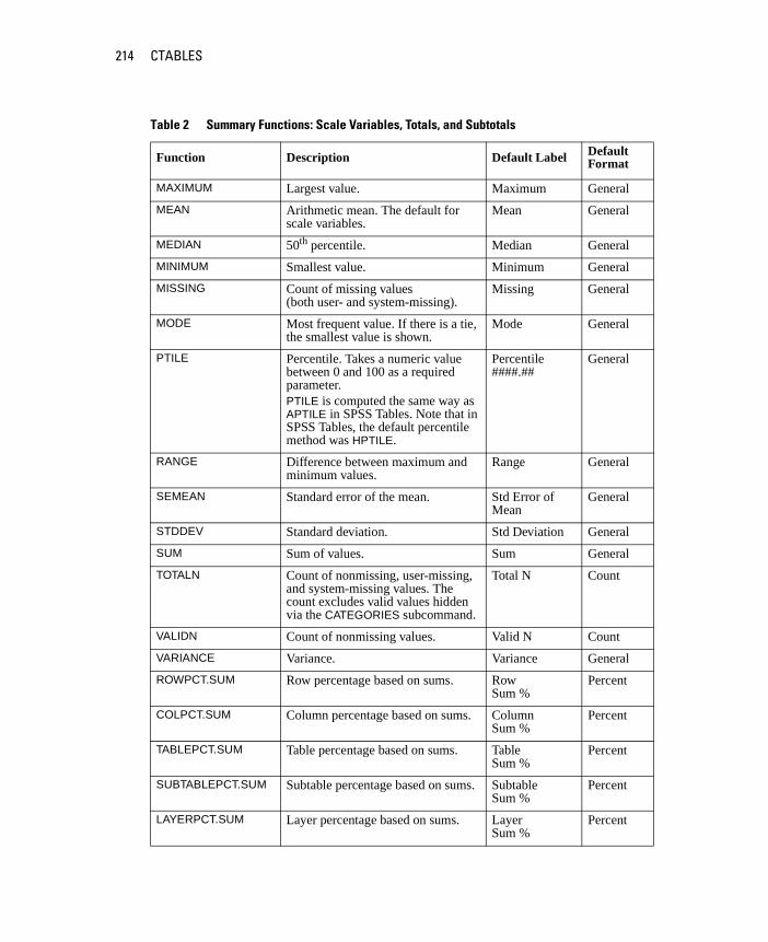
214 CTABLES
Table 2 Summary Functions: Scale Variables, Totals, and Subtotals
Function Description Default Label Default Format
MAXIMUM Largest value. Maximum General
MEAN Arithmetic mean. The default for scale variables.
Mean General
MEDIAN 50th percentile. Median General
MINIMUM Smallest value. Minimum General
MISSING Count of missing values (both user- and system-missing).
Missing General
MODE Most frequent value. If there is a tie, the smallest value is shown.
Mode General
PTILE Percentile. Takes a numeric value between 0 and 100 as a required parameter. PTILE is computed the same way as APTILE in SPSS Tables. Note that in SPSS Tables, the default percentile method was HPTILE.
Percentile####.##
General
RANGE Difference between maximum and minimum values.
Range General
SEMEAN Standard error of the mean. Std Error of Mean
General
STDDEV Standard deviation. Std Deviation General
SUM Sum of values. Sum General
TOTALN Count of nonmissing, user-missing, and system-missing values. The count excludes valid values hidden via the CATEGORIES subcommand.
Total N Count
VALIDN Count of nonmissing values. Valid N Count
VARIANCE Variance. Variance General
ROWPCT.SUM Row percentage based on sums. Row Sum %
Percent
COLPCT.SUM Column percentage based on sums. Column Sum %
Percent
TABLEPCT.SUM Table percentage based on sums. Table Sum %
Percent
SUBTABLEPCT.SUM Subtable percentage based on sums. SubtableSum %
Percent
LAYERPCT.SUM Layer percentage based on sums. Layer Sum %
Percent

CTABLES 215
Function Description Default Label Default Format
LAYERROWPCT. SUM Row percentage based on sums. Percentages sum to 100% across the entire row.
Layer Row Sum %
Percent
LAYERCOLPCT. SUM Column percentage based on sums. Percentages sum to 100% across the entire column.
LayerColumn Sum %
Percent
Table 3 Summary Functions: Multiple Response Sets
Function Description Default Label Default Format
RESPONSES Count of responses. Responses Count
ROWPCT.RESPONSES Row percentage based on responses. Total number of responses is the denominator.
RowResponses %
Percent
COLPCT.RESPONSES Column percentage based on responses. Total number of responses is the denominator.
ColumnResponses %
Percent
TABLEPCT.RESPONSES Table percentage based on responses. Total number of responses is the denominator.
TableResponses %
Percent
SUBTABLEPCT.RESPONSES Subtable percentage based on responses. Total number of responses is the denominator.
SubtableResponses %
Percent
LAYERPCT.RESPONSES Layer percentage based on responses. Total number of responses is the denominator.
LayerResponses %
Percent
LAYERROWPCT.RESPONSES Row percentage based on responses. Total number of responses is the denominator.Percentages sum to 100% across the entire row (that is, across subtables).
Layer RowResponses %
Percent
LAYERCOLPCT. RESPONSES Column percentage based on responses. Total number of responses is the denominator.Percentages sum to 100% across the entire column (that is, across subtables).
LayerColumnResponses %
Percent
Table 2 Summary Functions: Scale Variables, Totals, and Subtotals (Continued)

216 CTABLES
Function Description Default Label Default Format
ROWPCT.RESPONSES.COUNT Row percentage: responses are the numerator and total count is the denominator.
RowResponses %(Base: Count)
Percent
COLPCT.RESPONSES.COUNT Column percentage: responses are the numerator and total count is the denominator.
ColumnResponses %(Base: Count)
Percent
TABLEPCT.RESPONSES. COUNT Table percentage: responses are the numerator and total count is the denominator.
TableResponses %(Base: Count)
Percent
SUBTABLEPCT.RESPONSES. COUNT
Subtable percentage: responses are the numerator and total count is the denominator.
SubtableResponses %(Base: Count)
Percent
LAYERPCT. RESPONSES.COUNT Layer percentage: responses are the numerator and total count is the denominator.
LayerResponses %(Base: Count)
Percent
LAYERROWPCT.RESPONSES.COUNT
Row percentage: responses are the numerator and total count is the denominator.Percentages sum to 100% across the entire row (that is, across subtables).
Layer RowResponses %(Base: Count)
Percent
LAYERCOLPCT.RESPONSES.COUNT
Column percentage: responses are the numerator and total count is the denominator.Percentages sum to 100% across the entire column (that is, across subtables).
LayerColumnResponses %(Base: Count)
Percent
ROWPCT.COUNT.RESPONSES Row percentage: count is the numerator and total responses are the denominator.
Row Count %(Base: Responses)
Percent
COLPCT.COUNT.RESPONSES Column percentage: count is the numerator and total responses are the denominator.
ColumnCount %(Base: Responses)
Percent
TABLEPCT.COUNT. RESPONSES Table percentage: count is the numerator and total responses are the denominator.
Table Count %(Base: Responses)
Percent
Table 3 Summary Functions: Multiple Response Sets (Continued)
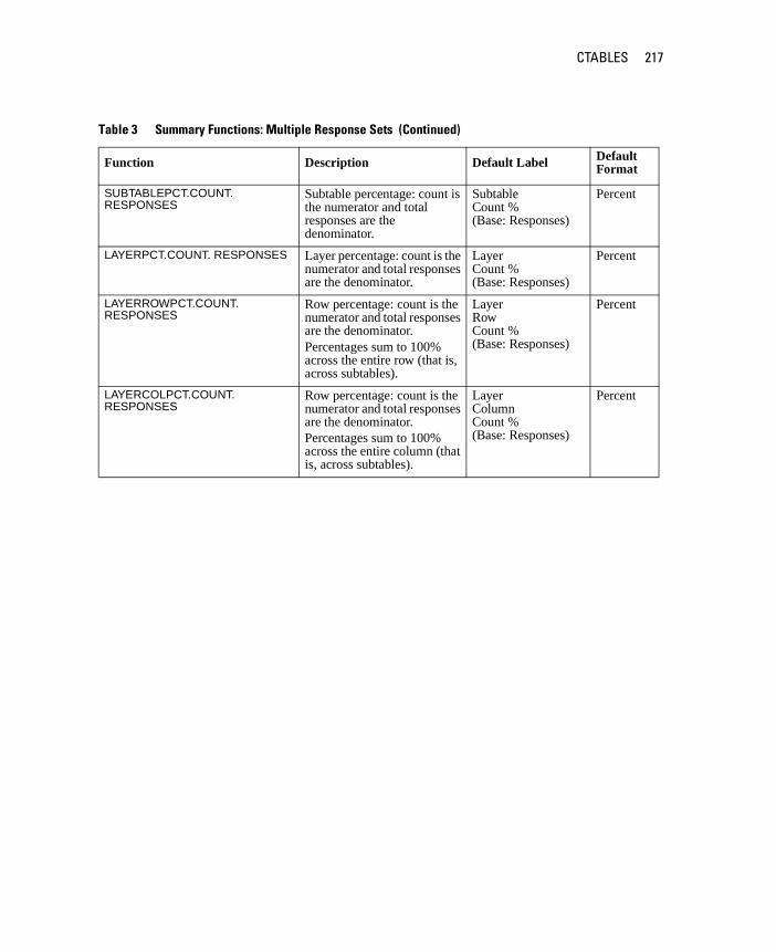
CTABLES 217
Function Description Default Label Default Format
SUBTABLEPCT.COUNT. RESPONSES
Subtable percentage: count is the numerator and total responses are the denominator.
SubtableCount %(Base: Responses)
Percent
LAYERPCT.COUNT. RESPONSES Layer percentage: count is the numerator and total responses are the denominator.
Layer Count %(Base: Responses)
Percent
LAYERROWPCT.COUNT. RESPONSES
Row percentage: count is the numerator and total responses are the denominator.Percentages sum to 100% across the entire row (that is, across subtables).
Layer Row Count % (Base: Responses)
Percent
LAYERCOLPCT.COUNT. RESPONSES
Row percentage: count is the numerator and total responses are the denominator.Percentages sum to 100% across the entire column (that is, across subtables).
LayerColumnCount %(Base: Responses)
Percent
Table 3 Summary Functions: Multiple Response Sets (Continued)

218 CTABLES
Formats for Summaries
A default format is assigned to each summary function:
Count The value is expressed in F (standard numeric) format with 0 decimal places. If youhave fractional weights and want a count that reflects those weights, use F formatwith appropriate decimal places.
Percent The value is expressed with one decimal place and a percent symbol.
General The value is expressed in the variable’s print format.
These default formats are internal to CTABLES and cannot be used in TABLE expressions. Tooverride the default formats, use any of the print formats available in the SPSS Base exceptZ, PBHEX, and HEX, or the additional formats described in Table 4.
Table 4 Additional Formats for Summaries
Format Description Example
NEGPARENw.d Parentheses appear around negative numbers.
–1234.567 formatted as NEGPAREN9.2 yields (1234.57).
NEQUALw.d “N=” precedes the number. 1234.567 formatted as NEQUAL9.2 yields N=1234.57.
PARENw.d The number is parenthesized. 1234.567 formatted as PAREN8.2 yields (1234.57).
PCTPARENw.d A percent symbol follows the value, which is parenthesized.
1234.567 formatted as PCTPAREN10.2 yields (1234.57%).

CTABLES 219
Missing Values in Summaries
Table 5 presents the rules for including cases in a table for VALIDN, COUNT, and TOTALNfunctions when values are included or excluded explicitly through an explicit category listor implicitly through inclusion or exclusion of user-missing values.
Table 5 Inclusion/Exclusion of Values in Summaries
Variable and Value Type VALIDN COUNT TOTALN
Categorical Variable: shown valid value
Multiple Dichotomy Set: at least one “true” value
Multiple Category Set: at least one shown valid value
Scale Variable: valid value
Include Include Include
Categorical Variable: included user-missing value
Multiple Category Set: all values are included user-missing
Scale Variable: user-missing or system-missing
Exclude Include Include
Categorical Variable: excluded user-missing or system-missing
Multiple Dichotomy Set: all values are “false”
Multiple Category Set: all values are excluded user-missing, system-missing, or excluded valid, but at least one value is not excluded valid
Exclude Exclude Include
Categorical Variable: excluded valid value
Multiple Dichotomy Set: all values are excluded valid values
Exclude Exclude Exclude
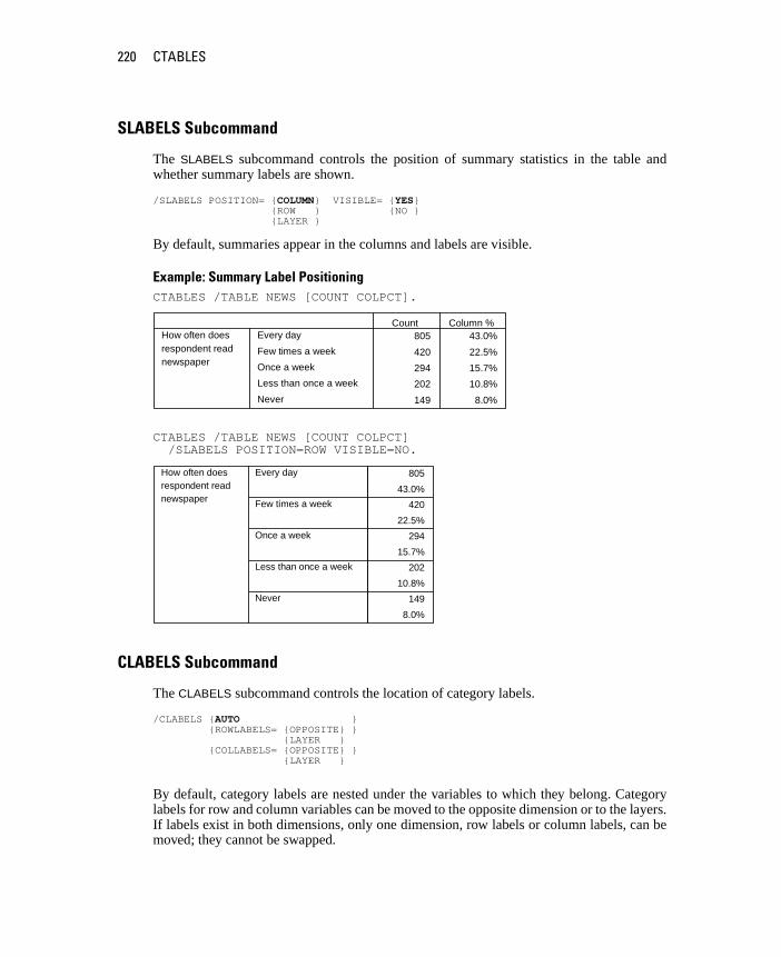
220 CTABLES
SLABELS Subcommand
The SLABELS subcommand controls the position of summary statistics in the table andwhether summary labels are shown.
/SLABELS POSITION= {COLUMN} VISIBLE= {YES} {ROW } {NO } {LAYER }
By default, summaries appear in the columns and labels are visible.
Example: Summary Label PositioningCTABLES /TABLE NEWS [COUNT COLPCT].
CTABLES /TABLE NEWS [COUNT COLPCT] /SLABELS POSITION=ROW VISIBLE=NO.
CLABELS Subcommand
The CLABELS subcommand controls the location of category labels.
/CLABELS {AUTO } {ROWLABELS= {OPPOSITE} } {LAYER } {COLLABELS= {OPPOSITE} } {LAYER }
By default, category labels are nested under the variables to which they belong. Categorylabels for row and column variables can be moved to the opposite dimension or to the layers.If labels exist in both dimensions, only one dimension, row labels or column labels, can bemoved; they cannot be swapped.
805 43.0%
420 22.5%
294 15.7%
202 10.8%
149 8.0%
Every day
Few times a week
Once a week
Less than once a week
Never
How often doesrespondent readnewspaper
Count Column %
805
43.0%
420
22.5%
294
15.7%
202
10.8%
149
8.0%
Every day
Few times a week
Once a week
Less than once a week
Never
How often doesrespondent readnewspaper
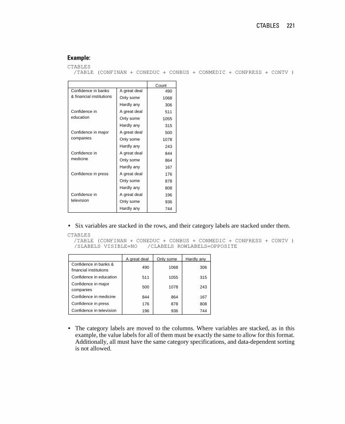
CTABLES 221
Example: CTABLES /TABLE (CONFINAN + CONEDUC + CONBUS + CONMEDIC + CONPRESS + CONTV )
• Six variables are stacked in the rows, and their category labels are stacked under them.
CTABLES /TABLE (CONFINAN + CONEDUC + CONBUS + CONMEDIC + CONPRESS + CONTV ) /SLABELS VISIBLE=NO /CLABELS ROWLABELS=OPPOSITE
• The category labels are moved to the columns. Where variables are stacked, as in thisexample, the value labels for all of them must be exactly the same to allow for this format.Additionally, all must have the same category specifications, and data-dependent sortingis not allowed.
490
1068
306
511
1055
315
500
1078
243
844
864
167
176
878
808
196
936
744
A great deal
Only some
Hardly any
Confidence in banks& financial institutions
A great deal
Only some
Hardly any
Confidence ineducation
A great deal
Only some
Hardly any
Confidence in majorcompanies
A great deal
Only some
Hardly any
Confidence inmedicine
A great deal
Only some
Hardly any
Confidence in press
A great deal
Only some
Hardly any
Confidence intelevision
Count
490 1068 306
511 1055 315
500 1078 243
844 864 167
176 878 808
196 936 744
Confidence in banks &financial institutions
Confidence in education
Confidence in majorcompanies
Confidence in medicine
Confidence in press
Confidence in television
A great deal Only some Hardly any
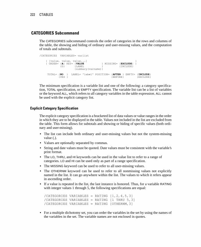
222 CTABLES
CATEGORIES Subcommand
The CATEGORIES subcommand controls the order of categories in the rows and columns ofthe table, the showing and hiding of ordinary and user-missing values, and the computationof totals and subtotals.
/CATEGORIES VARIABLES= varlist
{ [value, value, value...] } { ORDER= {A} KEY= {VALUE } MISSING= {EXCLUDE} } {D} {LABEL } {INCLUDE} {summary(varname)}
TOTAL= {NO } LABEL= "label" POSITION= {AFTER } EMPTY= {INCLUDE} {YES } {BEFORE} {EXCLUDE}
The minimum specification is a variable list and one of the following: a category specifica-tion, TOTAL specification, or EMPTY specification. The variable list can be a list of variablesor the keyword ALL, which refers to all category variables in the table expression. ALL cannotbe used with the explicit category list.
Explicit Category Specification
The explicit category specification is a bracketed list of data values or value ranges in the orderin which they are to be displayed in the table. Values not included in the list are excluded fromthe table. This form allows for subtotals and showing or hiding of specific values (both ordi-nary and user-missing).
• The list can include both ordinary and user-missing values but not the system-missingvalue (.).
• Values are optionally separated by commas.
• String and date values must be quoted. Date values must be consistent with the variable’sprint format.
• The LO, THRU, and HI keywords can be used in the value list to refer to a range of categories. LO and HI can be used only as part of a range specification.
• The MISSING keyword can be used to refer to all user-missing values. • The OTHERNM keyword can be used to refer to all nonmissing values not explicitly
named in the list. It can go anywhere within the list. The values to which it refers appearin ascending order.
• If a value is repeated in the list, the last instance is honored. Thus, for a variable RATINGwith integer values 1 through 5, the following specifications are equal:
/CATEGORIES VARIABLES = RATING [1,2,4,5,3]/CATEGORIES VARIABLES = RATING [1 THRU 5,3]/CATEGORIES VARIABLES = RATING [OTHERNM,3]
• For a multiple dichotomy set, you can order the variables in the set by using the names ofthe variables in the set. The variable names are not enclosed in quotes.
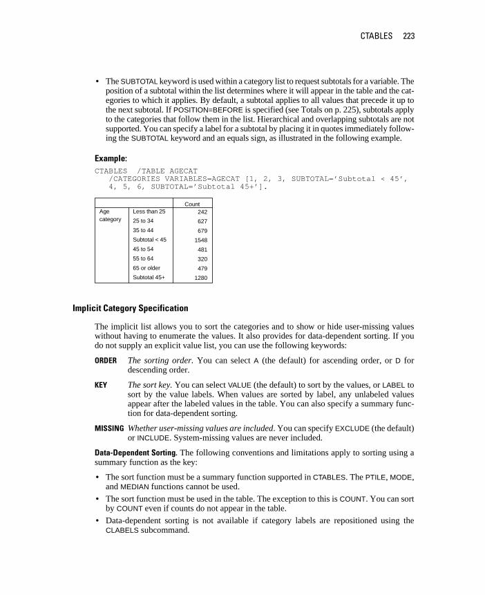
CTABLES 223
• The SUBTOTAL keyword is used within a category list to request subtotals for a variable. Theposition of a subtotal within the list determines where it will appear in the table and the cat-egories to which it applies. By default, a subtotal applies to all values that precede it up tothe next subtotal. If POSITION=BEFORE is specified (see Totals on p. 225), subtotals applyto the categories that follow them in the list. Hierarchical and overlapping subtotals are notsupported. You can specify a label for a subtotal by placing it in quotes immediately follow-ing the SUBTOTAL keyword and an equals sign, as illustrated in the following example.
Example:CTABLES /TABLE AGECAT /CATEGORIES VARIABLES=AGECAT [1, 2, 3, SUBTOTAL=’Subtotal < 45’, 4, 5, 6, SUBTOTAL=’Subtotal 45+’].
Implicit Category Specification
The implicit list allows you to sort the categories and to show or hide user-missing valueswithout having to enumerate the values. It also provides for data-dependent sorting. If youdo not supply an explicit value list, you can use the following keywords:
ORDER The sorting order. You can select A (the default) for ascending order, or D fordescending order.
KEY The sort key. You can select VALUE (the default) to sort by the values, or LABEL tosort by the value labels. When values are sorted by label, any unlabeled valuesappear after the labeled values in the table. You can also specify a summary func-tion for data-dependent sorting.
MISSING Whether user-missing values are included. You can specify EXCLUDE (the default)or INCLUDE. System-missing values are never included.
Data-Dependent Sorting. The following conventions and limitations apply to sorting using asummary function as the key:
• The sort function must be a summary function supported in CTABLES. The PTILE, MODE,and MEDIAN functions cannot be used.
• The sort function must be used in the table. The exception to this is COUNT. You can sortby COUNT even if counts do not appear in the table.
• Data-dependent sorting is not available if category labels are repositioned using theCLABELS subcommand.
242
627
679
1548
481
320
479
1280
Less than 25
25 to 34
35 to 44
Subtotal < 45
45 to 54
55 to 64
65 or older
Subtotal 45+
Agecategory
Count

224 CTABLES
• Summary functions available only for scale variables require that you give the variablename in parentheses, as in MEAN(AGE). Other functions, such as COUNT, do not requirea variable name, but you can supply one to restrict the sort.
• When a variable name is given and multiple logical tables are created through stacking,the entire table is sorted based on the first logical table that includes the categorical vari-able being sorted and the variable specified in the key.
• When a table contains more than one dimension, the sort is based on the distribution ofthe key within the categories of the sorted variable without regard to the contents of theother dimensions. Thus, given the table CTABLES /TABLE A BY B + C /CAT VAR=A ORDER=A KEY=COUNT(A),the rows are sorted according to the counts for the categories of A without regard to thevalues of B and C. If there are no missing values in the other dimension, the result is thesame as sorting on the totals for that dimension, in this case B or C. If the other dimensionhas an unbalanced pattern of missing values, the sorting may give unexpected results;however, the result is unaffected by differences in the pattern for B and C.
• If the sort variable is crossed with stacked category variables, the first table in the stackdetermines the sort order.
• To ensure that the categories are sorted the same way in each layer of the pivot table, layervariables are ignored for the purpose of sorting.
Example:CTABLES /TABLE CAR1 BY AGECAT /CATEGORIES VARIABLES=AGECAT TOTAL=YES /CATEGORIES VARIABLES=CAR1 ORDER=D KEY=COUNT.
• The first CATEGORIES subcommand requests a total across all age categories.
• The second CATEGORIES subcommand requests a sort of the categories of CAR1 indescending order using COUNT as the key. The categories of CAR1 are sorted accordingto the total counts.
99 267 293 214 140 215 1228
73 136 140 107 66 104 626
18 91 69 63 36 61 338
23 77 88 45 35 50 318
18 32 46 20 24 25 165
11 24 43 32 19 24 153
American
Japanese
German
Korean
Swedish
Other
Carmaker,mostrecentcar
Count
Less than25
Count
25 to 34
Count
35 to 44
Count
45 to 54
Count
55 to 64
Count
65 or older
Count
Total
Age category
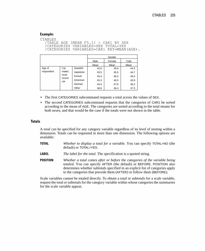
CTABLES 225
Example:CTABLES /TABLE AGE [MEAN F5.1] > CAR1 BY SEX /CATEGORIES VARIABLES=SEX TOTAL=YES /CATEGORIES VARIABLES=CAR1 KEY=MEAN(AGE).
• The first CATEGORIES subcommand requests a total across the values of SEX.
• The second CATEGORIES subcommand requests that the categories of CAR1 be sortedaccording to the mean of AGE. The categories are sorted according to the total means forboth sexes, and that would be the case if the totals were not shown in the table.
Totals
A total can be specified for any category variable regardless of its level of nesting within adimension. Totals can be requested in more than one dimension. The following options areavailable:
TOTAL Whether to display a total for a variable. You can specify TOTAL=NO (thedefault) or TOTAL=YES.
LABEL The label for the total. The specification is a quoted string.
POSITION Whether a total comes after or before the categories of the variable beingtotaled. You can specify AFTER (the default) or BEFORE. POSITION alsodetermines whether subtotals specified in an explicit list of categories applyto the categories that precede them (AFTER) or follow them (BEFORE).
Scale variables cannot be totaled directly. To obtain a total or subtotals for a scale variable,request the total or subtotals for the category variable within whose categories the summariesfor the scale variable appear.
42.6 45.6 44.3
43.5 45.5 44.7
43.4 46.2 45.0
45.3 46.5 45.9
44.3 47.6 46.2
48.6 46.4 47.3
Swedish
Japanese
Korean
American
German
Other
Carmaker,mostrecentcar
Age ofrespondent
Mean
Male
Mean
Female
Mean
Total
Gender
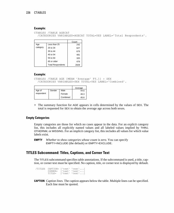
226 CTABLES
Example:CTABLES /TABLE AGECAT /CATEGORIES VARIABLES=AGECAT TOTAL=YES LABEL=’Total Respondents’.
Example:CTABLES /TABLE AGE [MEAN ’Average’ F5.1] > SEX /CATEGORIES VARIABLES=SEX TOTAL=YES LABEL=’Combined’.
• The summary function for AGE appears in cells determined by the values of SEX. Thetotal is requested for SEX to obtain the average age across both sexes.
Empty Categories
Empty categories are those for which no cases appear in the data. For an explicit categorylist, this includes all explicitly named values and all labeled values implied by THRU,OTHERNM, or MISSING. For an implicit category list, this includes all values for which valuelabels exist.
EMPTY Whether to show categories whose count is zero. You can specify EMPTY=INCLUDE (the default) or EMPTY=EXCLUDE.
TITLES Subcommand: Titles, Captions, and Corner Text
The TITLES subcommand specifies table annotations. If the subcommand is used, a title, cap-tion, or corner text must be specified. No caption, title, or corner text is displayed by default.
/TITLES CAPTION= [’text’ ’text’...] CORNER= [’text’ ’text’...] TITLE= [’text’ ’text’...]
CAPTION Caption lines. The caption appears below the table. Multiple lines can be specified.Each line must be quoted.
242
627
679
481
320
479
2828
Less than 25
25 to 34
35 to 44
45 to 54
55 to 64
65 or older
Total Respondents
Agecategory
Count
44.6
46.3
45.6
Male
Female
Combined
GenderAge ofrespondent
Average
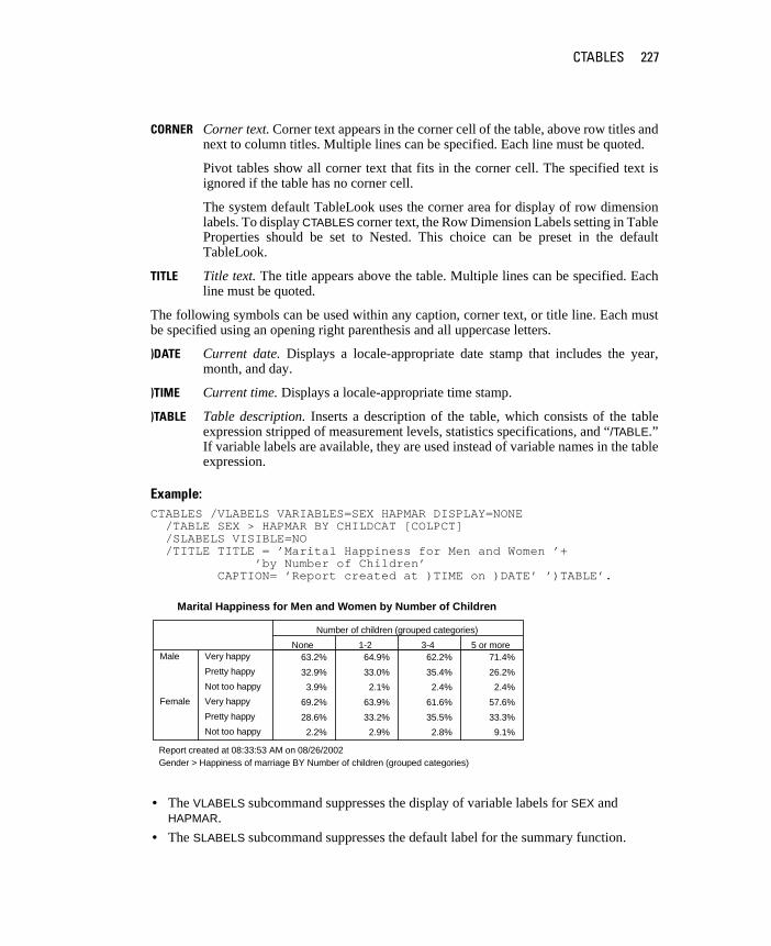
CTABLES 227
CORNER Corner text. Corner text appears in the corner cell of the table, above row titles andnext to column titles. Multiple lines can be specified. Each line must be quoted.
Pivot tables show all corner text that fits in the corner cell. The specified text isignored if the table has no corner cell.
The system default TableLook uses the corner area for display of row dimensionlabels. To display CTABLES corner text, the Row Dimension Labels setting in TableProperties should be set to Nested. This choice can be preset in the defaultTableLook.
TITLE Title text. The title appears above the table. Multiple lines can be specified. Eachline must be quoted.
The following symbols can be used within any caption, corner text, or title line. Each mustbe specified using an opening right parenthesis and all uppercase letters.
)DATE Current date. Displays a locale-appropriate date stamp that includes the year,month, and day.
)TIME Current time. Displays a locale-appropriate time stamp.
)TABLE Table description. Inserts a description of the table, which consists of the tableexpression stripped of measurement levels, statistics specifications, and “/TABLE.”If variable labels are available, they are used instead of variable names in the tableexpression.
Example:CTABLES /VLABELS VARIABLES=SEX HAPMAR DISPLAY=NONE /TABLE SEX > HAPMAR BY CHILDCAT [COLPCT] /SLABELS VISIBLE=NO /TITLE TITLE = ’Marital Happiness for Men and Women ’+ ’by Number of Children’ CAPTION= ’Report created at )TIME on )DATE’ ’)TABLE’.
• The VLABELS subcommand suppresses the display of variable labels for SEX and HAPMAR.
• The SLABELS subcommand suppresses the default label for the summary function.
Marital Happiness for Men and Women by Number of Children
63.2% 64.9% 62.2% 71.4%
32.9% 33.0% 35.4% 26.2%
3.9% 2.1% 2.4% 2.4%
69.2% 63.9% 61.6% 57.6%
28.6% 33.2% 35.5% 33.3%
2.2% 2.9% 2.8% 9.1%
Very happy
Pretty happy
Not too happy
Male
Very happy
Pretty happy
Not too happy
Female
None 1-2 3-4 5 or more
Number of children (grouped categories)
Report created at 08:33:53 AM on 08/26/2002Gender > Happiness of marriage BY Number of children (grouped categories)

228 CTABLES
• The TITLE specification on the TITLE subcommand uses the standard SPSS convention tobreak a single string across input lines.
• The CAPTION specification uses the )DATE, )TIME, and )TABLE keywords to print the date,time, and a description of the table structure.
Significance Testing
Custom Tables can perform the chi-square test of independence and pairwise comparisonsof column proportions for tables that contain at least one category variable in both the rowsand the columns, and pairwise comparisons of column means for tables that contain at leastone summary variable in the rows and one category variable in the columns.
Chi-Square Tests: SIGTEST Subcommand
/SIGTEST TYPE= CHISQUARE ALPHA= {0.05 } {significance level}
The SIGTEST subcommand has the following specifications:
TYPE The type of significance test. The specification is required. The only current choiceis CHISQUARE.
ALPHA The significance level for the test. The specification must be greater than 0 and lessthan 1. The default is 0.05.
Example: CTABLES /TABLE AGECAT BY MARITAL /CATEGORIES VARIABLES=AGECAT MARITAL TOTAL=YES /SIGTEST TYPE=CHISQUARE.
37 1 5 5 194 242
271 13 63 16 263 626
379 11 129 44 116 679
275 18 123 13 52 481
186 31 76 7 20 320
197 209 48 8 17 479
1345 283 444 93 662 2827
Less than 25
25 to 34
35 to 44
45 to 54
55 to 64
65 or older
Total
Agecategory
Count
Married
Count
Widowed
Count
Divorced
Count
Separated
Count
Nevermarried
Count
Total
Marital status
Pearson Chi-Square Tests
1473.381
20
.000*
Chi-square
df
Sig.
Agecategory
Marital status
Results are based on nonempty rows and columns in eachinnermost subtable.
The Chi-square statistic is significant at the 0.05 level.*.
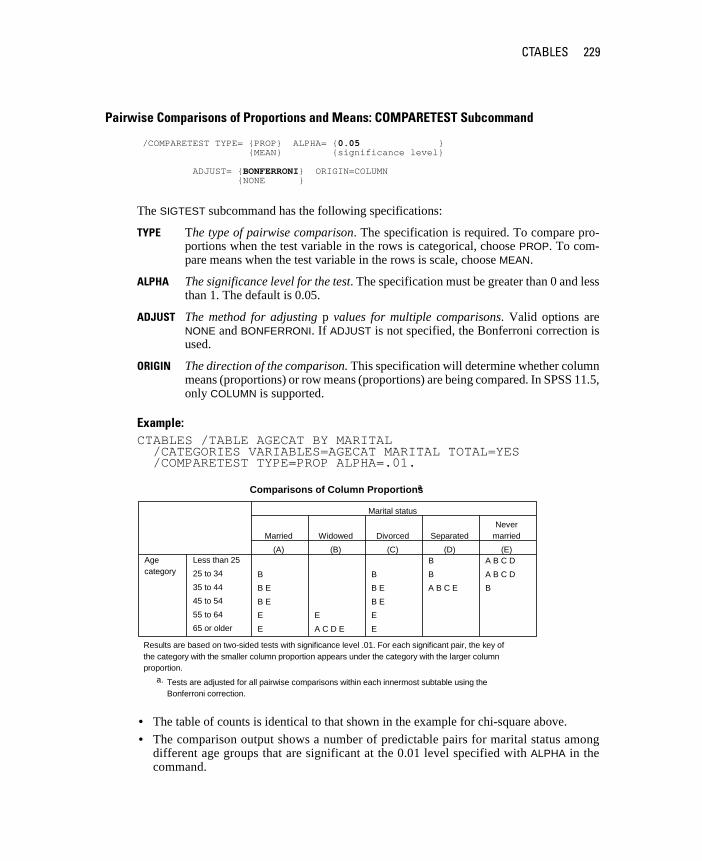
CTABLES 229
Pairwise Comparisons of Proportions and Means: COMPARETEST Subcommand
/COMPARETEST TYPE= {PROP} ALPHA= {0.05 } {MEAN} {significance level}
ADJUST= {BONFERRONI} ORIGIN=COLUMN {NONE }
The SIGTEST subcommand has the following specifications:
TYPE The type of pairwise comparison. The specification is required. To compare pro-portions when the test variable in the rows is categorical, choose PROP. To com-pare means when the test variable in the rows is scale, choose MEAN.
ALPHA The significance level for the test. The specification must be greater than 0 and lessthan 1. The default is 0.05.
ADJUST The method for adjusting p values for multiple comparisons. Valid options areNONE and BONFERRONI. If ADJUST is not specified, the Bonferroni correction isused.
ORIGIN The direction of the comparison. This specification will determine whether columnmeans (proportions) or row means (proportions) are being compared. In SPSS 11.5,only COLUMN is supported.
Example:CTABLES /TABLE AGECAT BY MARITAL /CATEGORIES VARIABLES=AGECAT MARITAL TOTAL=YES /COMPARETEST TYPE=PROP ALPHA=.01.
• The table of counts is identical to that shown in the example for chi-square above.
• The comparison output shows a number of predictable pairs for marital status amongdifferent age groups that are significant at the 0.01 level specified with ALPHA in thecommand.
Comparisons of Column Proportionsa
B A B C D
B B B A B C D
B E B E A B C E B
B E B E
E E E
E A C D E E
Less than 25
25 to 34
35 to 44
45 to 54
55 to 64
65 or older
Agecategory
(A)
Married
(B)
Widowed
(C)
Divorced
(D)
Separated
(E)
Nevermarried
Marital status
Results are based on two-sided tests with significance level .01. For each significant pair, the key ofthe category with the smaller column proportion appears under the category with the larger columnproportion.
Tests are adjusted for all pairwise comparisons within each innermost subtable using theBonferroni correction.
a.

230 CTABLES
Example:CTABLES /TABLE AGE > SEX BY MARITAL /CATEGORIES VARIABLES=SEX TOTAL=YES /COMPARETEST TYPE=MEAN.
FORMAT Subcommand
/FORMAT MINCOLWIDTH={DEFAULT} MAXCOLWIDTH={DEFAULT} {value } {value }
UNITS={POINTS} EMPTY= {ZERO } MISSING= {’.’ } {INCHES} {BLANK } {’chars’} {CM } {’chars’}
The FORMAT subcommand controls the appearance of the table. At least one of the followingattributes must be specified: MINCOLWIDTH, MAXCOLWIDTH, UNITS, EMPTY, or MISSING.
MINCOLWIDTH The minimum width of columns in the table. This includes the main tables aswell as any tables of significance tests. DEFAULT honors the column labelssetting in the current TableLook. The value must be less than or equal to thesetting for MAXCOLWIDTH.
MAXCOLWIDTH The maximum width of columns in the table. This includes the main tables aswell as any tables of significance tests. DEFAULT honors column labels set-ting in the current TableLook. The value must be greater than or equal to thesetting for MINCOLWIDTH.
UNITS The measurement system for column width values. The default is POINTS.You can also specify INCHES or CM (centimeters). UNITS is ignored unlessMINCOLWIDTH or MAXCOLWIDTH is specified.
49 66 48 44 32
45 70 48 41 32
47 70 48 42 32
Male
Female
Total
GenderAge ofrespondent
Mean
Married
Mean
Widowed
Mean
Divorced
Mean
Separated
Mean
Nevermarried
Marital status
Comparisons of Column Meansa
E A C D E E E
E A C D E D E E
Male
Female
GenderAge of respondent(A)
Married
(B)
Widowed
(C)
Divorced
(D)
Separated
(E)
Nevermarried
Marital status
Results are based on two-sided tests assuming equal variances with significance level 0.05. For each significantpair, the key of the smaller category appears under the category with larger mean.
Tests are adjusted for all pairwise comparisons within each innermost subtable using the Bonferronicorrection.
a.
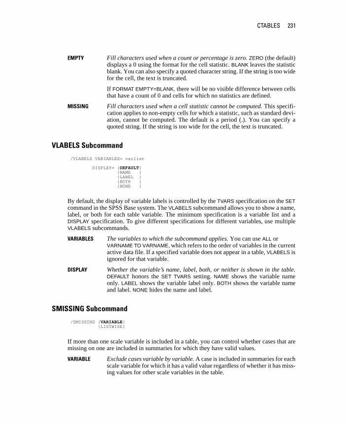
CTABLES 231
EMPTY Fill characters used when a count or percentage is zero. ZERO (the default)displays a 0 using the format for the cell statistic. BLANK leaves the statisticblank. You can also specify a quoted character string. If the string is too widefor the cell, the text is truncated.
If FORMAT EMPTY=BLANK, there will be no visible difference between cellsthat have a count of 0 and cells for which no statistics are defined.
MISSING Fill characters used when a cell statistic cannot be computed. This specifi-cation applies to non-empty cells for which a statistic, such as standard devi-ation, cannot be computed. The default is a period (.). You can specify aquoted string. If the string is too wide for the cell, the text is truncated.
VLABELS Subcommand
/VLABELS VARIABLES= varlist
DISPLAY= {DEFAULT} {NAME } {LABEL } {BOTH } {NONE }
By default, the display of variable labels is controlled by the TVARS specification on the SETcommand in the SPSS Base system. The VLABELS subcommand allows you to show a name,label, or both for each table variable. The minimum specification is a variable list and aDISPLAY specification. To give different specifications for different variables, use multipleVLABELS subcommands.
VARIABLES The variables to which the subcommand applies. You can use ALL or VARNAME TO VARNAME, which refers to the order of variables in the currentactive data file. If a specified variable does not appear in a table, VLABELS isignored for that variable.
DISPLAY Whether the variable’s name, label, both, or neither is shown in the table.DEFAULT honors the SET TVARS setting. NAME shows the variable nameonly. LABEL shows the variable label only. BOTH shows the variable nameand label. NONE hides the name and label.
SMISSING Subcommand
/SMISSING {VARIABLE} {LISTWISE}
If more than one scale variable is included in a table, you can control whether cases that aremissing on one are included in summaries for which they have valid values.
VARIABLE Exclude cases variable by variable. A case is included in summaries for eachscale variable for which it has a valid value regardless of whether it has miss-ing values for other scale variables in the table.
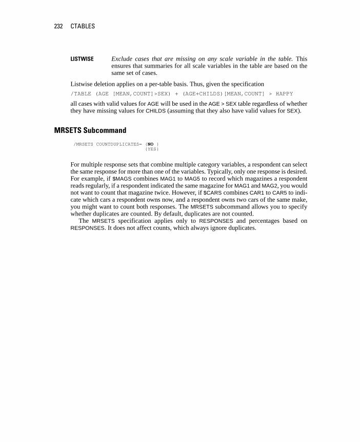
232 CTABLES
LISTWISE Exclude cases that are missing on any scale variable in the table. Thisensures that summaries for all scale variables in the table are based on thesame set of cases.
Listwise deletion applies on a per-table basis. Thus, given the specification
/TABLE (AGE [MEAN,COUNT]>SEX) + (AGE+CHILDS)[MEAN,COUNT] > HAPPY
all cases with valid values for AGE will be used in the AGE > SEX table regardless of whetherthey have missing values for CHILDS (assuming that they also have valid values for SEX).
MRSETS Subcommand
/MRSETS COUNTDUPLICATES= {NO } {YES}
For multiple response sets that combine multiple category variables, a respondent can selectthe same response for more than one of the variables. Typically, only one response is desired.For example, if $MAGS combines MAG1 to MAG5 to record which magazines a respondentreads regularly, if a respondent indicated the same magazine for MAG1 and MAG2, you wouldnot want to count that magazine twice. However, if $CARS combines CAR1 to CAR5 to indi-cate which cars a respondent owns now, and a respondent owns two cars of the same make,you might want to count both responses. The MRSETS subcommand allows you to specifywhether duplicates are counted. By default, duplicates are not counted.
The MRSETS specification applies only to RESPONSES and percentages based onRESPONSES. It does not affect counts, which always ignore duplicates.
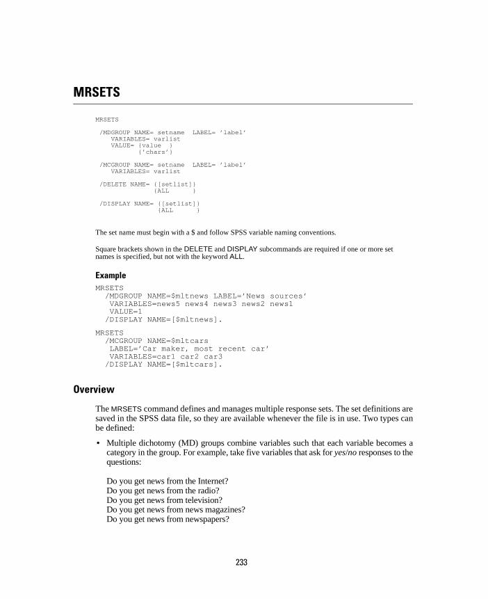
233
MRSETS
MRSETS
/MDGROUP NAME= setname LABEL= ’label’ VARIABLES= varlist VALUE= {value } {’chars’}
/MCGROUP NAME= setname LABEL= ’label’ VARIABLES= varlist
/DELETE NAME= {[setlist]} {ALL }
/DISPLAY NAME= {[setlist]} {ALL }
The set name must begin with a $ and follow SPSS variable naming conventions.
Square brackets shown in the DELETE and DISPLAY subcommands are required if one or more set names is specified, but not with the keyword ALL.
ExampleMRSETS /MDGROUP NAME=$mltnews LABEL=’News sources’ VARIABLES=news5 news4 news3 news2 news1 VALUE=1 /DISPLAY NAME=[$mltnews].
MRSETS /MCGROUP NAME=$mltcars LABEL=’Car maker, most recent car’ VARIABLES=car1 car2 car3 /DISPLAY NAME=[$mltcars].
Overview
The MRSETS command defines and manages multiple response sets. The set definitions aresaved in the SPSS data file, so they are available whenever the file is in use. Two types canbe defined:
• Multiple dichotomy (MD) groups combine variables such that each variable becomes acategory in the group. For example, take five variables that ask for yes/no responses to thequestions:
Do you get news from the Internet?Do you get news from the radio?Do you get news from television?Do you get news from news magazines?Do you get news from newspapers?
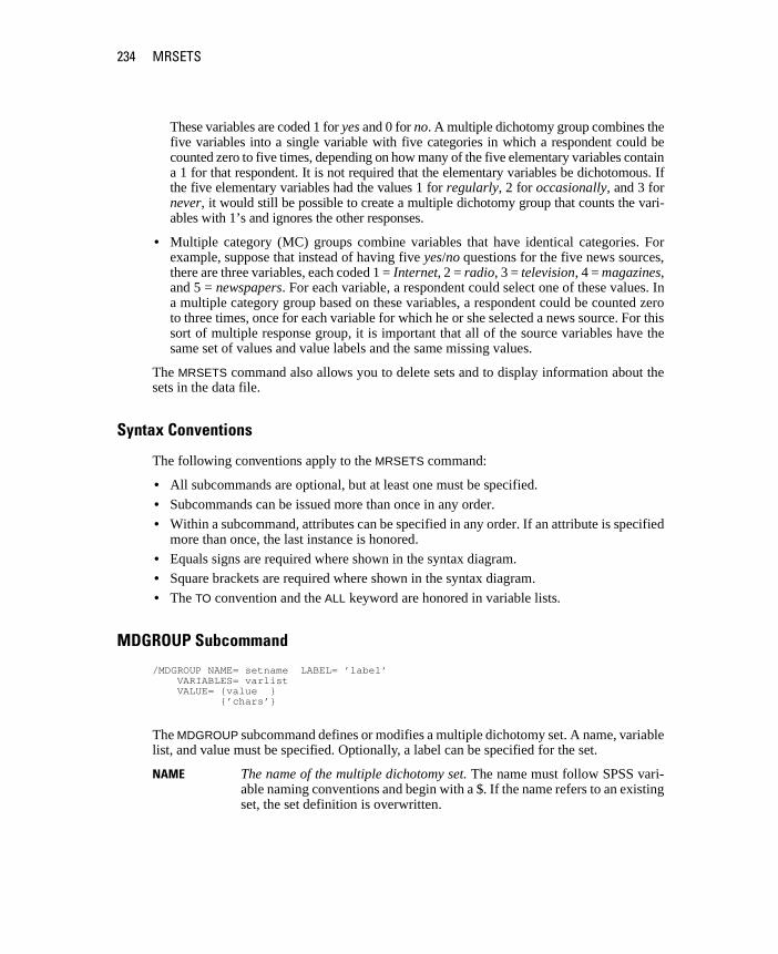
234 MRSETS
These variables are coded 1 for yes and 0 for no. A multiple dichotomy group combines thefive variables into a single variable with five categories in which a respondent could becounted zero to five times, depending on how many of the five elementary variables containa 1 for that respondent. It is not required that the elementary variables be dichotomous. Ifthe five elementary variables had the values 1 for regularly, 2 for occasionally, and 3 fornever, it would still be possible to create a multiple dichotomy group that counts the vari-ables with 1’s and ignores the other responses.
• Multiple category (MC) groups combine variables that have identical categories. Forexample, suppose that instead of having five yes/no questions for the five news sources,there are three variables, each coded 1 = Internet, 2 = radio, 3 = television, 4 = magazines,and 5 = newspapers. For each variable, a respondent could select one of these values. Ina multiple category group based on these variables, a respondent could be counted zeroto three times, once for each variable for which he or she selected a news source. For thissort of multiple response group, it is important that all of the source variables have thesame set of values and value labels and the same missing values.
The MRSETS command also allows you to delete sets and to display information about thesets in the data file.
Syntax Conventions
The following conventions apply to the MRSETS command:
• All subcommands are optional, but at least one must be specified.
• Subcommands can be issued more than once in any order.
• Within a subcommand, attributes can be specified in any order. If an attribute is specifiedmore than once, the last instance is honored.
• Equals signs are required where shown in the syntax diagram.• Square brackets are required where shown in the syntax diagram.
• The TO convention and the ALL keyword are honored in variable lists.
MDGROUP Subcommand
/MDGROUP NAME= setname LABEL= ’label’ VARIABLES= varlist VALUE= {value } {’chars’}
The MDGROUP subcommand defines or modifies a multiple dichotomy set. A name, variablelist, and value must be specified. Optionally, a label can be specified for the set.
NAME The name of the multiple dichotomy set. The name must follow SPSS vari-able naming conventions and begin with a $. If the name refers to an existingset, the set definition is overwritten.

MRSETS 235
LABEL The label for the set. The label must be quoted and cannot be wider than theSPSS limit for variable labels. By default, the set is unlabeled.
VARIABLES The list of elementary variables that define the set. Variables must be of thesame type (numeric or string). At least two variables must be specified.
VALUE The value that indicates presence of a response. This is also referred to as the“counted” value. If the set type is numeric, the counted value must be aninteger. If the set type is string, the counted value, after trimming trailingblanks, cannot be wider than the narrowest elementary variable.
Elementary variables need not have variable labels, but because variable labels are used asvalue labels for categories of the MD variable, a warning is issued if two or more variablesof an MD set have the same variable label. A warning is also issued if two or more elementaryvariables use different labels for the counted value—for example, if it is labeled Yes for Q1and No for Q2. When checking for label conflicts, case is ignored.
MCGROUP Subcommand
/MCGROUP NAME= setname LABEL= ’label’ VARIABLES= varlist
The MCGROUP subcommand defines or modifies a multiple category group. A name andvariable list must be specified. Optionally, a label can be specified for the set.
NAME The name of the multiple category set. The name must follow SPSS variablenaming conventions and begin with a $. If the name refers to an existing set,the set definition is overwritten.
LABEL The label for the set. The label must be quoted and cannot be wider than theSPSS limit for variable labels. By default, the set is unlabeled.
VARIABLES The list of elementary variables that define the set. Variables must be of thesame type (numeric or string). At least two variables must be specified.
The elementary variables need not have value labels, but a warning is issued if two or moreelementary variables have different labels for the same value. When checking for label con-flicts, case is ignored.
DELETE Subcommand
/DELETE NAME= {[setlist]} {ALL }
The DELETE subcommand deletes one or more set definitions. If one or more set names isgiven, the list must be enclosed in square brackets. ALL can be used to delete all sets; it is notenclosed in brackets.

236 MRSETS
DISPLAY Subcommand
/DISPLAY NAME= {[setlist]} {ALL }
The DISPLAY subcommand creates a table of information about one or more sets. If one ormore set names is given, the list must be enclosed in square brackets. ALL can be used to referto all sets; it is not enclosed in brackets.
237
Append ix
TABLES Command Syntax Converter
If you have command syntax files that contain TABLES syntax that you want to convert to CTABLES syntax, a simple utility program is provided to help you get started with the conversion process. There are, however, significant differences between TABLES and CTABLES functionality, and it is likely that you will find that the utility program cannot convert some of your TABLES syntax jobs or may generate CTABLES syntax that produces tables that do not closely resemble the original tables produced by the TABLES command. In most cases, you can edit the converted syntax to produce a table closely resembling the original.
The utility program is designed to:
� Create a new syntax file from an existing syntax file. The original syntax file is not altered.
� Convert only TABLES commands in the syntax file. Other commands in the file are not altered.
� Retain the original TABLES syntax in commented form.
� Identify the beginning and end of each conversion block with comments.
� Identify TABLES syntax commands that could not be converted.
� Convert command syntax files that follow either interactive or production mode syntax rules.
238
Appendix
The utility program may convert TABLES commands incorrectly under some circumstances, including TABLES commands that contain:
� Parenthesized variable names with the initial letters “sta” or “lab” in the TABLES subcommand if the variable is parenthesized by itself. For example, var1 by (statvar) by (labvar). These will be interpreted as the (STATISTICS) and (LABELS) keywords.
� SORT subcommands that use the abbreviations A or D to indicate ascending or descending sort order. These will be interpreted as variable names.
The utility program cannot convert TABLES commands that contain:
� Syntax errors.
� OBSERVATION subcommands that refer to a range of variables using the TO keyword (for example, var01 TO var05).
� String literals broken into segments separated by plus signs (for example, TITLE "My" + "Title").
� Macro calls that, in the absence of macro expansion, would be invalid TABLES syntax. Since the converter does not expand the macro calls, it treats them as if they were simply part of the standard TABLES syntax.
The utility program will not convert TABLES commands contained in macros. All macros are unaffected by the conversion process.
Using the Conversion Utility Program
The conversion utility program, syntaxconverter.exe, is installed in the same directory as SPSS. It is designed to run from a command prompt. The general form of the command is:
[SPSS install location]\syntaxconverter.exe [path]\inputfilename.sps [path]\outputfilename.sps
If any directory names contain spaces, enclose the entire path and filename in quotes, as in:
"c:\program files\spss\syntaxconverter.exe" c:\myfiles\oldfile.sps "c:\new files\newfile.sps"
239
TABLES Command Syntax Converter
Interactive versus Production Mode Command Syntax Rules
The conversion utility program can convert command files that use interactive or production mode syntax rules.
Interactive. The interactive syntax rules are:
� Each command begins on a new line.
� Each command ends with a period (.).
Production mode. The SPSS Production Facility and commands in files accessed via the INCLUDE command in a different command file use production mode syntax rules:
� Each command must begin in the first column of a new line.
� Continuation lines must be indented at least one space.
� The period at the end of the command is optional.
If your command files use production mode syntax rules and don’t contain periods at the end of each command, you need to include the command line switch -b (or /b) when you run syntaxconverter.exe, as in:
"c:\program files\spss\syntaxconverter.exe" -b c:\myfiles\oldfile.sps c:\myfiles\newfile.sps

241
S u b j e c t I n d e x
Bonferroni correctioncustom tables comparisons, 229
captionscustom tables, 51, 226
category labelspositioning in custom tables, 220
category specificationexplicit, in custom tables, 222implicit, in custom tables, 223
category variablescustom tables, 207
chi-square statisticscustom tables, 145
chi-square testcustom tables, 228
column means statisticscustom tables, 152
column proportions statisticscustom tables, 158
column widthcontrolling in custom tables, 48, 194custom tables, 230
comperimeter tables, 47, 103
concatenationcustom tables, 208
controlling number of decimals displayed, 63corner labels
custom tables, 51corner text
custom tables, 227count
vs. valid N, 134crosstabulation
custom tables, 61
custom tablescaptions, 51categorical variables, 26category label positioning, 220category variables, 207changing labels for summary statistics, 57changing measurement level, 26changing summary statistics dimension, 39column width, 48, 230compact view, 81comperimeter tables, 47, 103concatenation, 208controlling number of decimals displayed, 33corner labels, 51counting duplicate responses, 232crosstabulation, 61custom totals, 39display formats, 33empty cells, 48, 231excluding categories, 42, 66excluding valid values, 222hiding statistics labels, 56how to build a table, 29layer variables, 84, 87, 88listwise deletion, 231marginal totals, 64mean-frequency tables, 39missing summaries, 231missing values, 231missing values exclusion for scale summaries, 48multiple category sets, 48multiple response functions, 215multiple response sets, 26, 168, 207, 232nesting, 208nesting layer variables, 88nesting variables, 76, 81overview, 204percentage functions, 212percentages, 36, 37, 57, 62

242
Subject Index
percentages for multiple response sets, 37printing layered tables, 89reordering categories, 42row vs. column percentages, 57scale variable functions, 213scale variables, 26, 210showing and hiding variable names and labels, 33simple tables for categorical variables, 56sorting categories, 66stacking, 208stacking variables, 73, 75statistics source dimension, 62subtotals, 42, 91summary functions, 212summary label positioning, 220summary statistics, 36, 37, 38summary statistics display formats, 41swapping row and column variables, 83syntax conventions, 205table expression, 207table of frequencies, 47, 103tables of variables with shared categories, 47, 103test statistics, 52titles, 51totals, 42, 59, 91totals in tables with excluded categories, 66value labels for categorical variables, 26variable labels, 231variable types, 207
custom total summary statistics, 124
datescustom tables titles, 227including current date in custom tables, 51
decimalscontrolling number of decimals displayed in
custom tables, 33, 63, 188deleting categories
custom tables, 42, 66different summary statistics for different variables
stacked tables, 136display formats, 63
summary statistics in custom tables, 41, 188displaying category values, 128
duplicate responsescounting in custom tables, 232multiple category sets, 178
empty categoriesexcluding in custom tables, 226including in custom tables, 226
empty cellsdisplay format in custom tables, 231displayed value in custom tables, 48, 196
excluding categoriescustom tables, 42, 66
explicit category specificationcustom tables, 222
formats for summary functionscustom tables, 218
group totals, 95grouped summaries
scale variables, 139
hidingstatistics labels in custom tables, 56
implicit category specificationcustom tables, 223
labelschanging label text for summary statistics, 192positioning category labels in custom tables, 220positioning summary labels in custom tables, 220
layer variablescustom tables, 84, 87, 88nesting layer variables, 88
243
Subject Index
printing layered tables, 89stacking layer variables, 87
listwise deletioncustom tables, 231
maximumcustom tables, 38
mean, 132custom tables, 38
mean-frequency tables, 39, 124means
pairwise comparisons in custom tables, 229measurement level
changing in custom tables, 26median, 133
custom tables, 38minimum
custom tables, 38missing summary
custom tables, 231missing values, 134
custom tables, 219, 223, 231effect on percentage calculations, 184including in custom tables, 184
modecustom tables, 38
multiple category group, defined, 234
multiple dichotomy group, defined, 233multiple response sets
counts vs. responses, 170custom tables, 210, 232defining, 168duplicate responses in multiple category
sets, 48, 178functions in custom tables, 215multiple categories, 168multiple dichotomies, 168percentages, 37, 170responses, 170summary statistics source variable, 176totals, 170
nestingcustom tables, 208
nesting variablescustom tables, 76, 81scale variables, 142
omitting categoriescustom tables, 66
pairwise comparisonscomparison of means in custom tables, 229comparison of proportions in custom tables, 229custom tables, 229
percentage functionscustom tables, 212
percentagescustom tables, 36, 37, 57, 62missing values, 184multiple response sets, 37
percentilescustom tables, 214
position of totalscustom tables, 225
printingtables with layers, 89
proportionspairwise comparisons in custom tables, 229
rangecustom tables, 38
reordering categoriescustom tables, 42
scale variablescustom tables, 210functions in custom tables, 213grouped summaries, 139

244
Subject Index
multiple summary statistics, 133nesting, 142stacking, 132summaries grouped by row and column
categorical variables, 139summary statistics, 132totaling in custom tables, 225
significance testscustom tables, 52
sortingcustom tables, 223
sorting categoriescustom tables, 66
stackingcustom tables, 208multiple summary statistics source variables, 121
stacking variablescustom tables, 73, 75different summary statistics for different
variables, 136scale variables, 132stacking layer variables, 87
standard deviationcustom tables, 38
statisticscustom total summary statistics, 124stacked tables, 121
subgroup totals, 95
subtotals, 99custom tables, 42, 91, 223
sumcustom tables, 38
summariescustom tables, 210
summary labelscustom tables, 220
summary statisticschanging label text, 192custom total summary statistics, 124different summaries for different variables in
stacked tables, 136display format, 188multiple response sets, 170source dimension, 114source variable, 114
stacked tables, 121statistics, 114
summary statistics source variablemultiple response sets, 176scale variables, 142
table descriptioncustom tables titles, 227
table of frequenciescustom tables, 47, 103
TableLookschanging the default TableLook, 199
tablescustom tables, 26
test statisticscustom tables, 52
timeincluding current time in custom tables, 51
time stampcustom tables titles, 227
titlescustom tables, 51, 226
total N, 184totals
custom tables, 42, 59, 91, 225display position, 95excluded categories, 93group totals, 95layers, 98marginal totals for custom tables, 64nested tables, 95
unweighted functionscustom tables, 211
valid N, 134, 184custom tables, 38
valid valuesexcluding in custom tables, 222
245
Subject Index
valuesdisplaying category labels and values, 128
values and value labels, 128variable labels
custom tables, 231suppressing display in custom tables, 33
variable typescustom tables, 207
variancecustom tables, 38


247
S y n t a x I n d e x
BONFERRONI (keyword)CTABLES command, 229
CAPTION (keyword)CTABLES command, 226
CATEGORIES subcommandCTABLES command, 222
CHISQUARE (keyword)CTABLES command, 228
CLABELS (command)CATEGORIES subcommand, 222
CLABELS (subcommand)CTABLES command, 220
COMPARETEST (subcommand)CTABLES command, 229
CORNER (keyword)CTABLES command, 227
corner textCTABLES command, 227
COUNTDUPLICATES (keyword)CTABLES command, 232
CTABLES (command), 203CAPTION keyword, 226caption lines, 226CHISQUARE keyword, 228CLABELS subcommand, 220COMPARETEST subcommand, 229CORNER keyword, 227corner text, 227COUNTDUPLICATES keyword, 232)DATE keyword, 227dates in titles, 227empty categories, 226empty cell format, 230EMPTY keyword, 226, 230explicit category specification, 222FORMAT subcommand, 230formats for summaries, 218implicit category specification, 223
MISSING keyword, 223, 231missing values, 219, 223MRSETS subcommand, 232ORDER keyword, 223overview, 204position of totals, 225scale variable totals, 225SIGTEST subcommand, 228SLABELS subcommand, 220SMISSING subcommand, 231sorting categories, 223split file processing, 205subtotals, 223summary functions, 213summary functions for multiple response
sets, 215summary functions for scale variables, 213summary specifications, 210syntax conventions, 205table description in titles, 227)TABLE keyword, 227TABLE subcommand, 207)TIME keyword, 227TITLE keyword, 227TITLES subcommand, 226TOTAL keyword, 225totals, 225unweighted functions, 211variable types, 207VLABELS subcommand, 231
)DATE (keyword)CTABLES command, 227
EMPTY (keyword)CTABLES command, 230
explicit category specificationin CTABLES command, 222

248
Syntax Index
FORMAT (subcommand)CTABLES command, 230
implicit category specificationCTABLES command, 223
MCGROUP (subcommand)MRSETS command, 235
MDGROUP (subcommand)MRSETS command, 234
MISSING (keyword)CTABLES command, 223, 231
MRSETS (command), 233DELETE subcommand, 235DISPLAY subcommand, 236MCGROUP subcommand, 235MDGROUP subcommand, 234syntax conventions, 234
MRSETS (subcommand)CTABLES command, 232
ORDER (keyword)CTABLES command, 223
SIGTEST (subcommand)CTABLES command, 228
SLABELS (subcommand)CTABLES command, 220
SMISSING (subcommand)CTABLES command, 231
sorting categoriesCTABLES command, 223
)TABLE (keyword)CTABLES command, 227
TABLE subcommandCTABLES command, 207
)TIME keywordCTABLES command, 227
TITLES (subcommand)CTABLES command, 226
TOTAL (keyword)CTABLES command, 225
VLABELS (subcommand)CTABLES command, 231