SPSS 15.0 GPL Reference Guide - Kuwait University Reference Guide.pdf · SPSS 15.0 GPL Reference...

SPSS 15.0 GPL Reference Guide

For more information about SPSS® software products, please visit our Web site athttp://www.spss.com or contactSPSS Inc.233 South Wacker Drive, 11th FloorChicago, IL 60606-6412Tel: (312) 651-3000Fax: (312) 651-3668SPSS is a registered trademark and the other product names are the trademarks of SPSS Inc.for its proprietary computer software. No material describing such software may be producedor distributed without the written permission of the owners of the trademark and license rightsin the software and the copyrights in the published materials.The SOFTWARE and documentation are provided with RESTRICTED RIGHTS. Use,duplication, or disclosure by the Government is subject to restrictions as set forth in subdivision(c) (1) (ii) of The Rights in Technical Data and Computer Software clause at 52.227-7013.Contractor/manufacturer is SPSS Inc., 233 South Wacker Drive, 11th Floor, Chicago, IL60606-6412.Patent No. 7,023,453General notice: Other product names mentioned herein are used for identiÞcation purposes onlyand may be trademarks of their respective companies.TableLook is a trademark of SPSS Inc.Windows is a registered trademark of Microsoft Corporation.DataDirect, DataDirect Connect, INTERSOLV, and SequeLink are registered trademarks ofDataDirect Technologies.Portions of this product were created using LEADTOOLS © 1991�2000, LEAD Technologies,Inc. ALL RIGHTS RESERVED.LEAD, LEADTOOLS, and LEADVIEW are registered trademarks of LEAD Technologies, Inc.Sax Basic is a trademark of Sax Software Corporation. Copyright © 1993�2004 by PolarEngineering and Consulting. All rights reserved.A portion of the SPSS software contains zlib technology. Copyright © 1995�2002 by Jean-loupGailly and Mark Adler. The zlib software is provided �as is,� without express or implied warranty.A portion of the SPSS software contains Sun Java Runtime libraries. Copyright © 2003 by SunMicrosystems, Inc. All rights reserved. The Sun Java Runtime libraries include code licensedfrom RSA Security, Inc. Some portions of the libraries are licensed from IBM and are available athttp://www-128.ibm.com/developerworks/opensource/.SPSS 15.0 GPL Reference GuideCopyright © 2006 by SPSS Inc.All rights reserved.Printed in the United States of America.No part of this publication may be reproduced, stored in a retrieval system, or transmitted, in anyform or by any means, electronic, mechanical, photocopying, recording, or otherwise, withoutthe prior written permission of the publisher.

Contents

1 Introduction to GPL 1

The Basics . . . . . . . . . . . . . . . . . . . . . . . . . . . . . . . . . . . . . . . . . . . . . . . . . . . . . . . . . . . . . . . . . . 1Syntax Rules. . . . . . . . . . . . . . . . . . . . . . . . . . . . . . . . . . . . . . . . . . . . . . . . . . . . . . . . . . . . . . . . . 3Concepts . . . . . . . . . . . . . . . . . . . . . . . . . . . . . . . . . . . . . . . . . . . . . . . . . . . . . . . . . . . . . . . . . . . 3

Brief Overview of GPL Algebra. . . . . . . . . . . . . . . . . . . . . . . . . . . . . . . . . . . . . . . . . . . . . . . . 4How Coordinates and the Algebra Interact . . . . . . . . . . . . . . . . . . . . . . . . . . . . . . . . . . . . . . 7

Common Tasks . . . . . . . . . . . . . . . . . . . . . . . . . . . . . . . . . . . . . . . . . . . . . . . . . . . . . . . . . . . . . . 13How to Add Stacking to a Graph . . . . . . . . . . . . . . . . . . . . . . . . . . . . . . . . . . . . . . . . . . . . . 13How to Add Faceting (Paneling) to a Graph . . . . . . . . . . . . . . . . . . . . . . . . . . . . . . . . . . . . . 15How to Add Clustering to a Graph . . . . . . . . . . . . . . . . . . . . . . . . . . . . . . . . . . . . . . . . . . . . 17How to Use Aesthetics . . . . . . . . . . . . . . . . . . . . . . . . . . . . . . . . . . . . . . . . . . . . . . . . . . . . 18

What’s Changed in GPL. . . . . . . . . . . . . . . . . . . . . . . . . . . . . . . . . . . . . . . . . . . . . . . . . . . . . . . . 20

2 Statement and Function Reference 22

Statements . . . . . . . . . . . . . . . . . . . . . . . . . . . . . . . . . . . . . . . . . . . . . . . . . . . . . . . . . . . . . . . . . 22COMMENT Statement . . . . . . . . . . . . . . . . . . . . . . . . . . . . . . . . . . . . . . . . . . . . . . . . . . . . . 23PAGE Statement . . . . . . . . . . . . . . . . . . . . . . . . . . . . . . . . . . . . . . . . . . . . . . . . . . . . . . . . . 23GRAPH Statement . . . . . . . . . . . . . . . . . . . . . . . . . . . . . . . . . . . . . . . . . . . . . . . . . . . . . . . . 24SOURCE Statement . . . . . . . . . . . . . . . . . . . . . . . . . . . . . . . . . . . . . . . . . . . . . . . . . . . . . . . 25DATA Statement . . . . . . . . . . . . . . . . . . . . . . . . . . . . . . . . . . . . . . . . . . . . . . . . . . . . . . . . . 25TRANS Statement . . . . . . . . . . . . . . . . . . . . . . . . . . . . . . . . . . . . . . . . . . . . . . . . . . . . . . . . 26COORD Statement . . . . . . . . . . . . . . . . . . . . . . . . . . . . . . . . . . . . . . . . . . . . . . . . . . . . . . . . 26SCALE Statement. . . . . . . . . . . . . . . . . . . . . . . . . . . . . . . . . . . . . . . . . . . . . . . . . . . . . . . . . 31GUIDE Statement. . . . . . . . . . . . . . . . . . . . . . . . . . . . . . . . . . . . . . . . . . . . . . . . . . . . . . . . . 42ELEMENT Statement . . . . . . . . . . . . . . . . . . . . . . . . . . . . . . . . . . . . . . . . . . . . . . . . . . . . . . 47

Functions . . . . . . . . . . . . . . . . . . . . . . . . . . . . . . . . . . . . . . . . . . . . . . . . . . . . . . . . . . . . . . . . . . 58aestheticMaximum Function . . . . . . . . . . . . . . . . . . . . . . . . . . . . . . . . . . . . . . . . . . . . . . . . 60aestheticMinimum Function. . . . . . . . . . . . . . . . . . . . . . . . . . . . . . . . . . . . . . . . . . . . . . . . . 60aestheticMissing Function . . . . . . . . . . . . . . . . . . . . . . . . . . . . . . . . . . . . . . . . . . . . . . . . . . 61base Function . . . . . . . . . . . . . . . . . . . . . . . . . . . . . . . . . . . . . . . . . . . . . . . . . . . . . . . . . . . 62base.aesthetic Function. . . . . . . . . . . . . . . . . . . . . . . . . . . . . . . . . . . . . . . . . . . . . . . . . . . . 62base.all Function . . . . . . . . . . . . . . . . . . . . . . . . . . . . . . . . . . . . . . . . . . . . . . . . . . . . . . . . . 63base.coordinate Function . . . . . . . . . . . . . . . . . . . . . . . . . . . . . . . . . . . . . . . . . . . . . . . . . . 64begin Function (For Graphs) . . . . . . . . . . . . . . . . . . . . . . . . . . . . . . . . . . . . . . . . . . . . . . . . . 64begin Function (For Pages) . . . . . . . . . . . . . . . . . . . . . . . . . . . . . . . . . . . . . . . . . . . . . . . . . 65

iii

beta Function. . . . . . . . . . . . . . . . . . . . . . . . . . . . . . . . . . . . . . . . . . . . . . . . . . . . . . . . . . . . 65bin.dot Function . . . . . . . . . . . . . . . . . . . . . . . . . . . . . . . . . . . . . . . . . . . . . . . . . . . . . . . . . . 66bin.hex Function . . . . . . . . . . . . . . . . . . . . . . . . . . . . . . . . . . . . . . . . . . . . . . . . . . . . . . . . . 68bin.quantile.letter Function . . . . . . . . . . . . . . . . . . . . . . . . . . . . . . . . . . . . . . . . . . . . . . . . . 70bin.rect Function . . . . . . . . . . . . . . . . . . . . . . . . . . . . . . . . . . . . . . . . . . . . . . . . . . . . . . . . . 71binCount Function . . . . . . . . . . . . . . . . . . . . . . . . . . . . . . . . . . . . . . . . . . . . . . . . . . . . . . . . 73binStart Function . . . . . . . . . . . . . . . . . . . . . . . . . . . . . . . . . . . . . . . . . . . . . . . . . . . . . . . . . 74binWidth Function . . . . . . . . . . . . . . . . . . . . . . . . . . . . . . . . . . . . . . . . . . . . . . . . . . . . . . . . 74chiSquare Function . . . . . . . . . . . . . . . . . . . . . . . . . . . . . . . . . . . . . . . . . . . . . . . . . . . . . . . 75closed Function . . . . . . . . . . . . . . . . . . . . . . . . . . . . . . . . . . . . . . . . . . . . . . . . . . . . . . . . . . 76cluster Function. . . . . . . . . . . . . . . . . . . . . . . . . . . . . . . . . . . . . . . . . . . . . . . . . . . . . . . . . . 76col Function. . . . . . . . . . . . . . . . . . . . . . . . . . . . . . . . . . . . . . . . . . . . . . . . . . . . . . . . . . . . . 78collapse Function . . . . . . . . . . . . . . . . . . . . . . . . . . . . . . . . . . . . . . . . . . . . . . . . . . . . . . . . 79color Function (For Axes) . . . . . . . . . . . . . . . . . . . . . . . . . . . . . . . . . . . . . . . . . . . . . . . . . . . 80color Function (For Graphic Elements) . . . . . . . . . . . . . . . . . . . . . . . . . . . . . . . . . . . . . . . . . 81color.brightness Function. . . . . . . . . . . . . . . . . . . . . . . . . . . . . . . . . . . . . . . . . . . . . . . . . . . 82color.hue Function . . . . . . . . . . . . . . . . . . . . . . . . . . . . . . . . . . . . . . . . . . . . . . . . . . . . . . . . 84color.saturation Function . . . . . . . . . . . . . . . . . . . . . . . . . . . . . . . . . . . . . . . . . . . . . . . . . . . 85csvSource Function . . . . . . . . . . . . . . . . . . . . . . . . . . . . . . . . . . . . . . . . . . . . . . . . . . . . . . . 86dataMinimum Function . . . . . . . . . . . . . . . . . . . . . . . . . . . . . . . . . . . . . . . . . . . . . . . . . . . . 87dataMaximum Function . . . . . . . . . . . . . . . . . . . . . . . . . . . . . . . . . . . . . . . . . . . . . . . . . . . . 87delta Function . . . . . . . . . . . . . . . . . . . . . . . . . . . . . . . . . . . . . . . . . . . . . . . . . . . . . . . . . . . 87density.beta Function. . . . . . . . . . . . . . . . . . . . . . . . . . . . . . . . . . . . . . . . . . . . . . . . . . . . . . 88density.chiSquare Function . . . . . . . . . . . . . . . . . . . . . . . . . . . . . . . . . . . . . . . . . . . . . . . . . 89density.exponential Function . . . . . . . . . . . . . . . . . . . . . . . . . . . . . . . . . . . . . . . . . . . . . . . . 90density.f Function. . . . . . . . . . . . . . . . . . . . . . . . . . . . . . . . . . . . . . . . . . . . . . . . . . . . . . . . . 91density.gamma Function . . . . . . . . . . . . . . . . . . . . . . . . . . . . . . . . . . . . . . . . . . . . . . . . . . . 92density.kernel Function . . . . . . . . . . . . . . . . . . . . . . . . . . . . . . . . . . . . . . . . . . . . . . . . . . . . 93density.logistic Function . . . . . . . . . . . . . . . . . . . . . . . . . . . . . . . . . . . . . . . . . . . . . . . . . . . 95density.normal Function . . . . . . . . . . . . . . . . . . . . . . . . . . . . . . . . . . . . . . . . . . . . . . . . . . . . 96density.poisson Function . . . . . . . . . . . . . . . . . . . . . . . . . . . . . . . . . . . . . . . . . . . . . . . . . . . 97density.studentizedRange Function . . . . . . . . . . . . . . . . . . . . . . . . . . . . . . . . . . . . . . . . . . . 98density.t Function. . . . . . . . . . . . . . . . . . . . . . . . . . . . . . . . . . . . . . . . . . . . . . . . . . . . . . . . . 99density.uniform Function . . . . . . . . . . . . . . . . . . . . . . . . . . . . . . . . . . . . . . . . . . . . . . . . . . 100density.weibull Function . . . . . . . . . . . . . . . . . . . . . . . . . . . . . . . . . . . . . . . . . . . . . . . . . . 101dim Function . . . . . . . . . . . . . . . . . . . . . . . . . . . . . . . . . . . . . . . . . . . . . . . . . . . . . . . . . . . 102end Function . . . . . . . . . . . . . . . . . . . . . . . . . . . . . . . . . . . . . . . . . . . . . . . . . . . . . . . . . . . 104eval Function . . . . . . . . . . . . . . . . . . . . . . . . . . . . . . . . . . . . . . . . . . . . . . . . . . . . . . . . . . . 104exclude Function . . . . . . . . . . . . . . . . . . . . . . . . . . . . . . . . . . . . . . . . . . . . . . . . . . . . . . . . 108exponent Function . . . . . . . . . . . . . . . . . . . . . . . . . . . . . . . . . . . . . . . . . . . . . . . . . . . . . . . 109exponential Function . . . . . . . . . . . . . . . . . . . . . . . . . . . . . . . . . . . . . . . . . . . . . . . . . . . . . 109f Function . . . . . . . . . . . . . . . . . . . . . . . . . . . . . . . . . . . . . . . . . . . . . . . . . . . . . . . . . . . . . 110format Function . . . . . . . . . . . . . . . . . . . . . . . . . . . . . . . . . . . . . . . . . . . . . . . . . . . . . . . . . 110from Function . . . . . . . . . . . . . . . . . . . . . . . . . . . . . . . . . . . . . . . . . . . . . . . . . . . . . . . . . . 111

iv

gamma Function . . . . . . . . . . . . . . . . . . . . . . . . . . . . . . . . . . . . . . . . . . . . . . . . . . . . . . . . 111gap Function . . . . . . . . . . . . . . . . . . . . . . . . . . . . . . . . . . . . . . . . . . . . . . . . . . . . . . . . . . . 112gridlines Function . . . . . . . . . . . . . . . . . . . . . . . . . . . . . . . . . . . . . . . . . . . . . . . . . . . . . . . 112in Function. . . . . . . . . . . . . . . . . . . . . . . . . . . . . . . . . . . . . . . . . . . . . . . . . . . . . . . . . . . . . 112include Function . . . . . . . . . . . . . . . . . . . . . . . . . . . . . . . . . . . . . . . . . . . . . . . . . . . . . . . . 113index Function . . . . . . . . . . . . . . . . . . . . . . . . . . . . . . . . . . . . . . . . . . . . . . . . . . . . . . . . . . 114iter Function . . . . . . . . . . . . . . . . . . . . . . . . . . . . . . . . . . . . . . . . . . . . . . . . . . . . . . . . . . . 114jump Function . . . . . . . . . . . . . . . . . . . . . . . . . . . . . . . . . . . . . . . . . . . . . . . . . . . . . . . . . . 115label Function (For Graphic Elements) . . . . . . . . . . . . . . . . . . . . . . . . . . . . . . . . . . . . . . . . 115label Function (For Guides) . . . . . . . . . . . . . . . . . . . . . . . . . . . . . . . . . . . . . . . . . . . . . . . . 117layout.circle Function . . . . . . . . . . . . . . . . . . . . . . . . . . . . . . . . . . . . . . . . . . . . . . . . . . . . 117layout.dag Function . . . . . . . . . . . . . . . . . . . . . . . . . . . . . . . . . . . . . . . . . . . . . . . . . . . . . . 119layout.grid Function . . . . . . . . . . . . . . . . . . . . . . . . . . . . . . . . . . . . . . . . . . . . . . . . . . . . . . 120layout.network Function. . . . . . . . . . . . . . . . . . . . . . . . . . . . . . . . . . . . . . . . . . . . . . . . . . . 121layout.random Function . . . . . . . . . . . . . . . . . . . . . . . . . . . . . . . . . . . . . . . . . . . . . . . . . . . 122layout.tree Function . . . . . . . . . . . . . . . . . . . . . . . . . . . . . . . . . . . . . . . . . . . . . . . . . . . . . . 123link.alpha Function. . . . . . . . . . . . . . . . . . . . . . . . . . . . . . . . . . . . . . . . . . . . . . . . . . . . . . . 125link.complete Function . . . . . . . . . . . . . . . . . . . . . . . . . . . . . . . . . . . . . . . . . . . . . . . . . . . . 126link.delaunay Function . . . . . . . . . . . . . . . . . . . . . . . . . . . . . . . . . . . . . . . . . . . . . . . . . . . . 128link.distance Function . . . . . . . . . . . . . . . . . . . . . . . . . . . . . . . . . . . . . . . . . . . . . . . . . . . . 129link.gabriel Function. . . . . . . . . . . . . . . . . . . . . . . . . . . . . . . . . . . . . . . . . . . . . . . . . . . . . . 131link.hull Function . . . . . . . . . . . . . . . . . . . . . . . . . . . . . . . . . . . . . . . . . . . . . . . . . . . . . . . . 132link.influence Function . . . . . . . . . . . . . . . . . . . . . . . . . . . . . . . . . . . . . . . . . . . . . . . . . . . . 134link.join Function . . . . . . . . . . . . . . . . . . . . . . . . . . . . . . . . . . . . . . . . . . . . . . . . . . . . . . . . 135link.mst Function . . . . . . . . . . . . . . . . . . . . . . . . . . . . . . . . . . . . . . . . . . . . . . . . . . . . . . . . 137link.neighbor Function . . . . . . . . . . . . . . . . . . . . . . . . . . . . . . . . . . . . . . . . . . . . . . . . . . . . 138link.relativeNeighborhood Function . . . . . . . . . . . . . . . . . . . . . . . . . . . . . . . . . . . . . . . . . . 140link.sequence Function . . . . . . . . . . . . . . . . . . . . . . . . . . . . . . . . . . . . . . . . . . . . . . . . . . . 141link.tsp Function. . . . . . . . . . . . . . . . . . . . . . . . . . . . . . . . . . . . . . . . . . . . . . . . . . . . . . . . . 143logistic Function . . . . . . . . . . . . . . . . . . . . . . . . . . . . . . . . . . . . . . . . . . . . . . . . . . . . . . . . 144map Function. . . . . . . . . . . . . . . . . . . . . . . . . . . . . . . . . . . . . . . . . . . . . . . . . . . . . . . . . . . 145mapSource Function . . . . . . . . . . . . . . . . . . . . . . . . . . . . . . . . . . . . . . . . . . . . . . . . . . . . . 146mapVariables Function . . . . . . . . . . . . . . . . . . . . . . . . . . . . . . . . . . . . . . . . . . . . . . . . . . . 146marron Function . . . . . . . . . . . . . . . . . . . . . . . . . . . . . . . . . . . . . . . . . . . . . . . . . . . . . . . . 147max Function . . . . . . . . . . . . . . . . . . . . . . . . . . . . . . . . . . . . . . . . . . . . . . . . . . . . . . . . . . . 147min Function . . . . . . . . . . . . . . . . . . . . . . . . . . . . . . . . . . . . . . . . . . . . . . . . . . . . . . . . . . . 148mirror Function . . . . . . . . . . . . . . . . . . . . . . . . . . . . . . . . . . . . . . . . . . . . . . . . . . . . . . . . . 148missing.gap Function . . . . . . . . . . . . . . . . . . . . . . . . . . . . . . . . . . . . . . . . . . . . . . . . . . . . . 149missing.interpolate Function . . . . . . . . . . . . . . . . . . . . . . . . . . . . . . . . . . . . . . . . . . . . . . . 149missing.wings Function . . . . . . . . . . . . . . . . . . . . . . . . . . . . . . . . . . . . . . . . . . . . . . . . . . . 150noConstant Function . . . . . . . . . . . . . . . . . . . . . . . . . . . . . . . . . . . . . . . . . . . . . . . . . . . . . 150node Function . . . . . . . . . . . . . . . . . . . . . . . . . . . . . . . . . . . . . . . . . . . . . . . . . . . . . . . . . . 150notIn Function . . . . . . . . . . . . . . . . . . . . . . . . . . . . . . . . . . . . . . . . . . . . . . . . . . . . . . . . . . 151normal Function. . . . . . . . . . . . . . . . . . . . . . . . . . . . . . . . . . . . . . . . . . . . . . . . . . . . . . . . . 151

v

opposite Function . . . . . . . . . . . . . . . . . . . . . . . . . . . . . . . . . . . . . . . . . . . . . . . . . . . . . . . 152origin Function (For Graphs). . . . . . . . . . . . . . . . . . . . . . . . . . . . . . . . . . . . . . . . . . . . . . . . 152origin Function (For Scales) . . . . . . . . . . . . . . . . . . . . . . . . . . . . . . . . . . . . . . . . . . . . . . . . 153poisson Function . . . . . . . . . . . . . . . . . . . . . . . . . . . . . . . . . . . . . . . . . . . . . . . . . . . . . . . . 154position Function . . . . . . . . . . . . . . . . . . . . . . . . . . . . . . . . . . . . . . . . . . . . . . . . . . . . . . . . 154preserveStraightLines Function . . . . . . . . . . . . . . . . . . . . . . . . . . . . . . . . . . . . . . . . . . . . . 156project Function. . . . . . . . . . . . . . . . . . . . . . . . . . . . . . . . . . . . . . . . . . . . . . . . . . . . . . . . . 156proportion Function . . . . . . . . . . . . . . . . . . . . . . . . . . . . . . . . . . . . . . . . . . . . . . . . . . . . . . 157reflect Function . . . . . . . . . . . . . . . . . . . . . . . . . . . . . . . . . . . . . . . . . . . . . . . . . . . . . . . . . 157region.confi.count Function . . . . . . . . . . . . . . . . . . . . . . . . . . . . . . . . . . . . . . . . . . . . . . . . 158region.confi.mean Function . . . . . . . . . . . . . . . . . . . . . . . . . . . . . . . . . . . . . . . . . . . . . . . . 159region.confi.percent.count Function. . . . . . . . . . . . . . . . . . . . . . . . . . . . . . . . . . . . . . . . . . 161region.confi.smooth Function. . . . . . . . . . . . . . . . . . . . . . . . . . . . . . . . . . . . . . . . . . . . . . . 162region.spread.range Function . . . . . . . . . . . . . . . . . . . . . . . . . . . . . . . . . . . . . . . . . . . . . . 163region.spread.sd Function . . . . . . . . . . . . . . . . . . . . . . . . . . . . . . . . . . . . . . . . . . . . . . . . . 165region.spread.se Function . . . . . . . . . . . . . . . . . . . . . . . . . . . . . . . . . . . . . . . . . . . . . . . . . 166reverse Function . . . . . . . . . . . . . . . . . . . . . . . . . . . . . . . . . . . . . . . . . . . . . . . . . . . . . . . . 168root Function . . . . . . . . . . . . . . . . . . . . . . . . . . . . . . . . . . . . . . . . . . . . . . . . . . . . . . . . . . . 168sameRatio Function . . . . . . . . . . . . . . . . . . . . . . . . . . . . . . . . . . . . . . . . . . . . . . . . . . . . . . 169scale Function (For Axes). . . . . . . . . . . . . . . . . . . . . . . . . . . . . . . . . . . . . . . . . . . . . . . . . . 169scale Function (For Graphs) . . . . . . . . . . . . . . . . . . . . . . . . . . . . . . . . . . . . . . . . . . . . . . . . 170scale Function (For Graphic Elements) . . . . . . . . . . . . . . . . . . . . . . . . . . . . . . . . . . . . . . . . 170scale Function (For Pages). . . . . . . . . . . . . . . . . . . . . . . . . . . . . . . . . . . . . . . . . . . . . . . . . 171segments Function . . . . . . . . . . . . . . . . . . . . . . . . . . . . . . . . . . . . . . . . . . . . . . . . . . . . . . 172shape Function . . . . . . . . . . . . . . . . . . . . . . . . . . . . . . . . . . . . . . . . . . . . . . . . . . . . . . . . . 172showAll Function . . . . . . . . . . . . . . . . . . . . . . . . . . . . . . . . . . . . . . . . . . . . . . . . . . . . . . . . 173size Function . . . . . . . . . . . . . . . . . . . . . . . . . . . . . . . . . . . . . . . . . . . . . . . . . . . . . . . . . . . 173smooth.cubic Function. . . . . . . . . . . . . . . . . . . . . . . . . . . . . . . . . . . . . . . . . . . . . . . . . . . . 175smooth.linear Function . . . . . . . . . . . . . . . . . . . . . . . . . . . . . . . . . . . . . . . . . . . . . . . . . . . 176smooth.loess Function . . . . . . . . . . . . . . . . . . . . . . . . . . . . . . . . . . . . . . . . . . . . . . . . . . . . 178smooth.mean Function. . . . . . . . . . . . . . . . . . . . . . . . . . . . . . . . . . . . . . . . . . . . . . . . . . . . 179smooth.median Function . . . . . . . . . . . . . . . . . . . . . . . . . . . . . . . . . . . . . . . . . . . . . . . . . . 180smooth.spline Function . . . . . . . . . . . . . . . . . . . . . . . . . . . . . . . . . . . . . . . . . . . . . . . . . . . 182smooth.step Function. . . . . . . . . . . . . . . . . . . . . . . . . . . . . . . . . . . . . . . . . . . . . . . . . . . . . 183smooth.quadratic Function . . . . . . . . . . . . . . . . . . . . . . . . . . . . . . . . . . . . . . . . . . . . . . . . 183sort.data Function . . . . . . . . . . . . . . . . . . . . . . . . . . . . . . . . . . . . . . . . . . . . . . . . . . . . . . . 185sort.natural Function . . . . . . . . . . . . . . . . . . . . . . . . . . . . . . . . . . . . . . . . . . . . . . . . . . . . . 185sort.statistic Function . . . . . . . . . . . . . . . . . . . . . . . . . . . . . . . . . . . . . . . . . . . . . . . . . . . . 186sort.values Function. . . . . . . . . . . . . . . . . . . . . . . . . . . . . . . . . . . . . . . . . . . . . . . . . . . . . . 187split Function . . . . . . . . . . . . . . . . . . . . . . . . . . . . . . . . . . . . . . . . . . . . . . . . . . . . . . . . . . . 187start Function . . . . . . . . . . . . . . . . . . . . . . . . . . . . . . . . . . . . . . . . . . . . . . . . . . . . . . . . . . 188startAngle Function . . . . . . . . . . . . . . . . . . . . . . . . . . . . . . . . . . . . . . . . . . . . . . . . . . . . . . 189studentizedRange Function . . . . . . . . . . . . . . . . . . . . . . . . . . . . . . . . . . . . . . . . . . . . . . . . 189summary.count Function . . . . . . . . . . . . . . . . . . . . . . . . . . . . . . . . . . . . . . . . . . . . . . . . . . 190

vi

summary.count.cumulative Function . . . . . . . . . . . . . . . . . . . . . . . . . . . . . . . . . . . . . . . . . 191summary.max Function . . . . . . . . . . . . . . . . . . . . . . . . . . . . . . . . . . . . . . . . . . . . . . . . . . . 193summary.mean Function . . . . . . . . . . . . . . . . . . . . . . . . . . . . . . . . . . . . . . . . . . . . . . . . . . 195summary.min Function . . . . . . . . . . . . . . . . . . . . . . . . . . . . . . . . . . . . . . . . . . . . . . . . . . . . 196summary.percent Function. . . . . . . . . . . . . . . . . . . . . . . . . . . . . . . . . . . . . . . . . . . . . . . . . 198summary.percent.count . . . . . . . . . . . . . . . . . . . . . . . . . . . . . . . . . . . . . . . . . . . . . . . . . . . 198summary.percent.count.cumulative Function . . . . . . . . . . . . . . . . . . . . . . . . . . . . . . . . . . . 200summary.percent.cumulative Function. . . . . . . . . . . . . . . . . . . . . . . . . . . . . . . . . . . . . . . . 201summary.percent.sum . . . . . . . . . . . . . . . . . . . . . . . . . . . . . . . . . . . . . . . . . . . . . . . . . . . . 202summary.percent.sum.cumulative Function . . . . . . . . . . . . . . . . . . . . . . . . . . . . . . . . . . . . 203summary.sum Function . . . . . . . . . . . . . . . . . . . . . . . . . . . . . . . . . . . . . . . . . . . . . . . . . . . 205summary.sum.cumulative Function . . . . . . . . . . . . . . . . . . . . . . . . . . . . . . . . . . . . . . . . . . 206t Function . . . . . . . . . . . . . . . . . . . . . . . . . . . . . . . . . . . . . . . . . . . . . . . . . . . . . . . . . . . . . 208texture.pattern Function. . . . . . . . . . . . . . . . . . . . . . . . . . . . . . . . . . . . . . . . . . . . . . . . . . . 208ticks Function . . . . . . . . . . . . . . . . . . . . . . . . . . . . . . . . . . . . . . . . . . . . . . . . . . . . . . . . . . 209to Function . . . . . . . . . . . . . . . . . . . . . . . . . . . . . . . . . . . . . . . . . . . . . . . . . . . . . . . . . . . . 210transparency Function . . . . . . . . . . . . . . . . . . . . . . . . . . . . . . . . . . . . . . . . . . . . . . . . . . . . 210transpose Function . . . . . . . . . . . . . . . . . . . . . . . . . . . . . . . . . . . . . . . . . . . . . . . . . . . . . . 212uniform Function . . . . . . . . . . . . . . . . . . . . . . . . . . . . . . . . . . . . . . . . . . . . . . . . . . . . . . . . 212unit.percent Function. . . . . . . . . . . . . . . . . . . . . . . . . . . . . . . . . . . . . . . . . . . . . . . . . . . . . 213userSource Function . . . . . . . . . . . . . . . . . . . . . . . . . . . . . . . . . . . . . . . . . . . . . . . . . . . . . 213values Function . . . . . . . . . . . . . . . . . . . . . . . . . . . . . . . . . . . . . . . . . . . . . . . . . . . . . . . . . 214weibull Function . . . . . . . . . . . . . . . . . . . . . . . . . . . . . . . . . . . . . . . . . . . . . . . . . . . . . . . . 214weight Function . . . . . . . . . . . . . . . . . . . . . . . . . . . . . . . . . . . . . . . . . . . . . . . . . . . . . . . . . 215wrap Function . . . . . . . . . . . . . . . . . . . . . . . . . . . . . . . . . . . . . . . . . . . . . . . . . . . . . . . . . . 215

3 Examples 217

Using the Examples in Your Application. . . . . . . . . . . . . . . . . . . . . . . . . . . . . . . . . . . . . . . . . . . 217Summary Bar Chart Examples. . . . . . . . . . . . . . . . . . . . . . . . . . . . . . . . . . . . . . . . . . . . . . . . . . 218

Simple Bar Chart . . . . . . . . . . . . . . . . . . . . . . . . . . . . . . . . . . . . . . . . . . . . . . . . . . . . . . . . 218Simple Bar Chart of Counts . . . . . . . . . . . . . . . . . . . . . . . . . . . . . . . . . . . . . . . . . . . . . . . . 219Simple Horizontal Bar Chart . . . . . . . . . . . . . . . . . . . . . . . . . . . . . . . . . . . . . . . . . . . . . . . . 219Simple Bar Chart With Error Bars. . . . . . . . . . . . . . . . . . . . . . . . . . . . . . . . . . . . . . . . . . . . 220Simple Bar Chart with Bar for All Categories . . . . . . . . . . . . . . . . . . . . . . . . . . . . . . . . . . . 221Stacked Bar Chart . . . . . . . . . . . . . . . . . . . . . . . . . . . . . . . . . . . . . . . . . . . . . . . . . . . . . . . 222Clustered Bar Chart . . . . . . . . . . . . . . . . . . . . . . . . . . . . . . . . . . . . . . . . . . . . . . . . . . . . . . 223Clustered and Stacked Bar Chart . . . . . . . . . . . . . . . . . . . . . . . . . . . . . . . . . . . . . . . . . . . . 224Bar Chart Using an Evaluation Function . . . . . . . . . . . . . . . . . . . . . . . . . . . . . . . . . . . . . . . 225Bar Chart with Mapped Aesthetics . . . . . . . . . . . . . . . . . . . . . . . . . . . . . . . . . . . . . . . . . . 226Faceted (Paneled) Bar Chart . . . . . . . . . . . . . . . . . . . . . . . . . . . . . . . . . . . . . . . . . . . . . . . 227

vii

3-D Bar Chart. . . . . . . . . . . . . . . . . . . . . . . . . . . . . . . . . . . . . . . . . . . . . . . . . . . . . . . . . . . 229Error Bar Chart . . . . . . . . . . . . . . . . . . . . . . . . . . . . . . . . . . . . . . . . . . . . . . . . . . . . . . . . . 230

Histogram Examples . . . . . . . . . . . . . . . . . . . . . . . . . . . . . . . . . . . . . . . . . . . . . . . . . . . . . . . . . 231Histogram . . . . . . . . . . . . . . . . . . . . . . . . . . . . . . . . . . . . . . . . . . . . . . . . . . . . . . . . . . . . . 231Histogram with Distribution Curve . . . . . . . . . . . . . . . . . . . . . . . . . . . . . . . . . . . . . . . . . . . 231Percentage Histogram . . . . . . . . . . . . . . . . . . . . . . . . . . . . . . . . . . . . . . . . . . . . . . . . . . . . 233Frequency Polygon . . . . . . . . . . . . . . . . . . . . . . . . . . . . . . . . . . . . . . . . . . . . . . . . . . . . . . 233Stacked Histogram . . . . . . . . . . . . . . . . . . . . . . . . . . . . . . . . . . . . . . . . . . . . . . . . . . . . . . 234Faceted (Paneled) Histogram. . . . . . . . . . . . . . . . . . . . . . . . . . . . . . . . . . . . . . . . . . . . . . . 235Population Pyramid . . . . . . . . . . . . . . . . . . . . . . . . . . . . . . . . . . . . . . . . . . . . . . . . . . . . . . 235Cumulative Histogram . . . . . . . . . . . . . . . . . . . . . . . . . . . . . . . . . . . . . . . . . . . . . . . . . . . . 2363-D Histogram . . . . . . . . . . . . . . . . . . . . . . . . . . . . . . . . . . . . . . . . . . . . . . . . . . . . . . . . . . 237

High-Low Chart Examples . . . . . . . . . . . . . . . . . . . . . . . . . . . . . . . . . . . . . . . . . . . . . . . . . . . . . 237Simple Range Bar for One Variable . . . . . . . . . . . . . . . . . . . . . . . . . . . . . . . . . . . . . . . . . . 237Simple Range Bar for Two Variables . . . . . . . . . . . . . . . . . . . . . . . . . . . . . . . . . . . . . . . . . 238High-Low-Close Chart . . . . . . . . . . . . . . . . . . . . . . . . . . . . . . . . . . . . . . . . . . . . . . . . . . . . 239Difference Area Chart . . . . . . . . . . . . . . . . . . . . . . . . . . . . . . . . . . . . . . . . . . . . . . . . . . . . 239

Scatter/Dot Examples . . . . . . . . . . . . . . . . . . . . . . . . . . . . . . . . . . . . . . . . . . . . . . . . . . . . . . . . 240Simple 1-D Scatterplot . . . . . . . . . . . . . . . . . . . . . . . . . . . . . . . . . . . . . . . . . . . . . . . . . . . . 240Simple 2-D Scatterplot . . . . . . . . . . . . . . . . . . . . . . . . . . . . . . . . . . . . . . . . . . . . . . . . . . . . 241Simple 2-D Scatterplot with Fit Line . . . . . . . . . . . . . . . . . . . . . . . . . . . . . . . . . . . . . . . . . . 242Grouped Scatterplot . . . . . . . . . . . . . . . . . . . . . . . . . . . . . . . . . . . . . . . . . . . . . . . . . . . . . 242Grouped Scatterplot with Convex Hull . . . . . . . . . . . . . . . . . . . . . . . . . . . . . . . . . . . . . . . . 243Scatterplot Matrix (SPLOM) . . . . . . . . . . . . . . . . . . . . . . . . . . . . . . . . . . . . . . . . . . . . . . . . 244Bubble Plot . . . . . . . . . . . . . . . . . . . . . . . . . . . . . . . . . . . . . . . . . . . . . . . . . . . . . . . . . . . . 245Binned Scatterplot. . . . . . . . . . . . . . . . . . . . . . . . . . . . . . . . . . . . . . . . . . . . . . . . . . . . . . . 246Binned Scatterplot with Polygons . . . . . . . . . . . . . . . . . . . . . . . . . . . . . . . . . . . . . . . . . . . 247Scatterplot with Border Histograms . . . . . . . . . . . . . . . . . . . . . . . . . . . . . . . . . . . . . . . . . . 247Scatterplot with Border Boxplots . . . . . . . . . . . . . . . . . . . . . . . . . . . . . . . . . . . . . . . . . . . . 248Dot Plot . . . . . . . . . . . . . . . . . . . . . . . . . . . . . . . . . . . . . . . . . . . . . . . . . . . . . . . . . . . . . . . 2492-D Dot Plot . . . . . . . . . . . . . . . . . . . . . . . . . . . . . . . . . . . . . . . . . . . . . . . . . . . . . . . . . . . . 250Jittered Categorical Scatterplot . . . . . . . . . . . . . . . . . . . . . . . . . . . . . . . . . . . . . . . . . . . . . 252

Line Chart Examples . . . . . . . . . . . . . . . . . . . . . . . . . . . . . . . . . . . . . . . . . . . . . . . . . . . . . . . . . 252Simple Line Chart. . . . . . . . . . . . . . . . . . . . . . . . . . . . . . . . . . . . . . . . . . . . . . . . . . . . . . . . 252Simple Line Chart with Points. . . . . . . . . . . . . . . . . . . . . . . . . . . . . . . . . . . . . . . . . . . . . . . 253Line Chart of Date Data . . . . . . . . . . . . . . . . . . . . . . . . . . . . . . . . . . . . . . . . . . . . . . . . . . . 254Line Chart With Step Interpolation . . . . . . . . . . . . . . . . . . . . . . . . . . . . . . . . . . . . . . . . . . . 254Fit Line. . . . . . . . . . . . . . . . . . . . . . . . . . . . . . . . . . . . . . . . . . . . . . . . . . . . . . . . . . . . . . . . 255Line Chart from Equation . . . . . . . . . . . . . . . . . . . . . . . . . . . . . . . . . . . . . . . . . . . . . . . . . . 256Line Chart with Separate Scales . . . . . . . . . . . . . . . . . . . . . . . . . . . . . . . . . . . . . . . . . . . . 257Line Chart in Parallel Coordinates . . . . . . . . . . . . . . . . . . . . . . . . . . . . . . . . . . . . . . . . . . . 258

viii

Pie Chart Examples. . . . . . . . . . . . . . . . . . . . . . . . . . . . . . . . . . . . . . . . . . . . . . . . . . . . . . . . . . 259Pie Chart . . . . . . . . . . . . . . . . . . . . . . . . . . . . . . . . . . . . . . . . . . . . . . . . . . . . . . . . . . . . . . 259Paneled Pie Chart . . . . . . . . . . . . . . . . . . . . . . . . . . . . . . . . . . . . . . . . . . . . . . . . . . . . . . . 261

Boxplot Examples . . . . . . . . . . . . . . . . . . . . . . . . . . . . . . . . . . . . . . . . . . . . . . . . . . . . . . . . . . . 2611-D Boxplot . . . . . . . . . . . . . . . . . . . . . . . . . . . . . . . . . . . . . . . . . . . . . . . . . . . . . . . . . . . . 261Boxplot . . . . . . . . . . . . . . . . . . . . . . . . . . . . . . . . . . . . . . . . . . . . . . . . . . . . . . . . . . . . . . . 262Clustered Boxplot . . . . . . . . . . . . . . . . . . . . . . . . . . . . . . . . . . . . . . . . . . . . . . . . . . . . . . . 263Boxplot With Overlaid Dot Plot . . . . . . . . . . . . . . . . . . . . . . . . . . . . . . . . . . . . . . . . . . . . . . 264

Multi-Graph Examples . . . . . . . . . . . . . . . . . . . . . . . . . . . . . . . . . . . . . . . . . . . . . . . . . . . . . . . 265Scatterplot with Border Histograms . . . . . . . . . . . . . . . . . . . . . . . . . . . . . . . . . . . . . . . . . . 265Scatterplot with Border Boxplots . . . . . . . . . . . . . . . . . . . . . . . . . . . . . . . . . . . . . . . . . . . . 266Stocks Line Chart with Volume Bar Chart . . . . . . . . . . . . . . . . . . . . . . . . . . . . . . . . . . . . . . 267Dual Axis Graph. . . . . . . . . . . . . . . . . . . . . . . . . . . . . . . . . . . . . . . . . . . . . . . . . . . . . . . . . 268Histogram with Dot Plot . . . . . . . . . . . . . . . . . . . . . . . . . . . . . . . . . . . . . . . . . . . . . . . . . . . 269

Other Examples . . . . . . . . . . . . . . . . . . . . . . . . . . . . . . . . . . . . . . . . . . . . . . . . . . . . . . . . . . . . 270Collapsing Small Categories. . . . . . . . . . . . . . . . . . . . . . . . . . . . . . . . . . . . . . . . . . . . . . . . 270Mapping Aesthetics. . . . . . . . . . . . . . . . . . . . . . . . . . . . . . . . . . . . . . . . . . . . . . . . . . . . . . 271Faceting by Separate Variables . . . . . . . . . . . . . . . . . . . . . . . . . . . . . . . . . . . . . . . . . . . . . 272Grouping by Separate Variables. . . . . . . . . . . . . . . . . . . . . . . . . . . . . . . . . . . . . . . . . . . . . 273Clustering Separate Variables . . . . . . . . . . . . . . . . . . . . . . . . . . . . . . . . . . . . . . . . . . . . . . 274Binning over Categorical Values . . . . . . . . . . . . . . . . . . . . . . . . . . . . . . . . . . . . . . . . . . . . 275Categorical Heat Map . . . . . . . . . . . . . . . . . . . . . . . . . . . . . . . . . . . . . . . . . . . . . . . . . . . . 276Creating Categories Using the eval Function . . . . . . . . . . . . . . . . . . . . . . . . . . . . . . . . . . . 278

Appendix

A GPL Constants 279

Color Constants . . . . . . . . . . . . . . . . . . . . . . . . . . . . . . . . . . . . . . . . . . . . . . . . . . . . . . . . . . . . 279Shape Constants . . . . . . . . . . . . . . . . . . . . . . . . . . . . . . . . . . . . . . . . . . . . . . . . . . . . . . . . . . . 280Size Constants . . . . . . . . . . . . . . . . . . . . . . . . . . . . . . . . . . . . . . . . . . . . . . . . . . . . . . . . . . . . . 280Pattern Constants . . . . . . . . . . . . . . . . . . . . . . . . . . . . . . . . . . . . . . . . . . . . . . . . . . . . . . . . . . . 280

ix

Bibliography 281

Index 282

x

Chapter

1111Introduction to GPL

The Graphics Production Language (GPL) is a language for creating graphs. It is a conciseand ßexible language based on the grammar described in The Grammar of Graphics. Ratherthan requiring you to learn commands that are speciÞc to different graph types, GPL provides abasic grammar with which you can build any graph. For more information about the theory thatsupports GPL, see The Grammar of Graphics, 2nd Edition (Wilkinson, 2005).

Note: If you have used GPL previously, refer to What�s Changed in GPL on p. 20.

The Basics

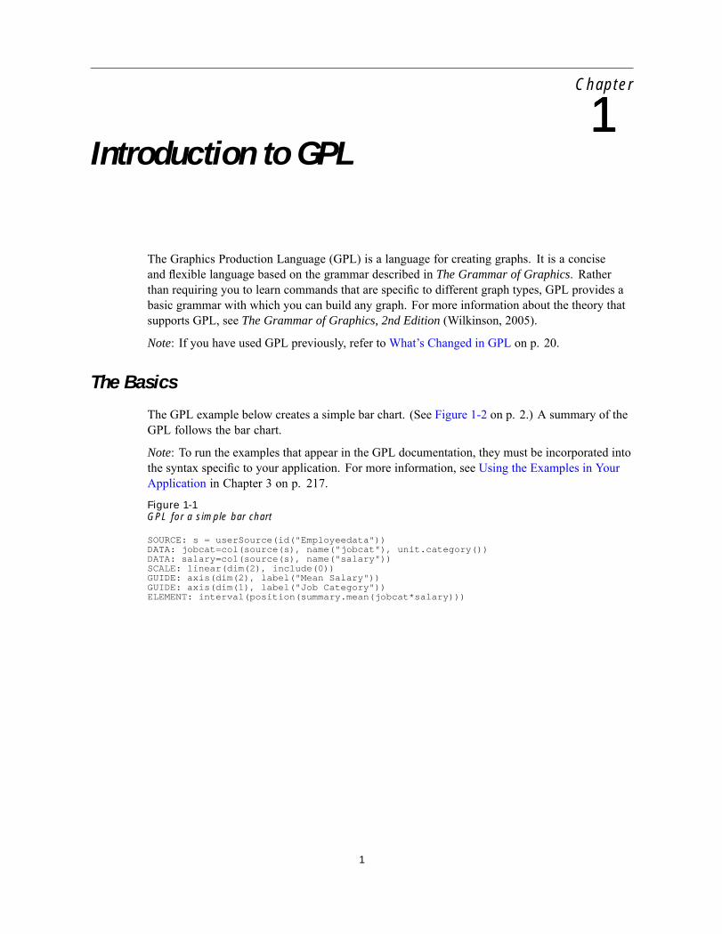
The GPL example below creates a simple bar chart. (See Figure 1-2 on p. 2.) A summary of theGPL follows the bar chart.

Note: To run the examples that appear in the GPL documentation, they must be incorporated intothe syntax speciÞc to your application. For more information, see Using the Examples in YourApplication in Chapter 3 on p. 217.

Figure 1-1GPL for a simple bar chart

SOURCE: s = userSource(id("Employeedata"))DATA: jobcat=col(source(s), name("jobcat"), unit.category())DATA: salary=col(source(s), name("salary"))SCALE: linear(dim(2), include(0))GUIDE: axis(dim(2), label("Mean Salary"))GUIDE: axis(dim(1), label("Job Category"))ELEMENT: interval(position(summary.mean(jobcat*salary)))

1

2

Chapter 1

Figure 1-2Simple bar chart

Each line in the example is a statement. One or more statements make up a block of GPL. Eachstatement speciÞes an aspect of the graph, such as the source data, relevant data transformations,coordinate systems, guides (for example, axis labels), graphic elements (for example, points andlines), and statistics.Statements begin with a label that identiÞes the statement type. The label and colon (:) that

follow it are the only items that delineate the statement.

Consider the statements in the example:! SOURCE. This statement speciÞes the Þle or dataset that contains the data for the graph. In the

example, it identiÞes userSource, which is a data source deÞned by the application that iscalling the GPL. The data source could also have been a comma-separated values (CSV) Þle.

! DATA. This statement assigns a variable to a column or Þeld in the data source. In theexample, the DATA statements assign jobcat and salary to two columns in the data source.The statement identiÞes the appropriate columns in the data source by using the namefunction. The strings passed to the name function correspond to variable names in theuserSource. These could also be the column header strings that appear in the Þrst line of aCSV Þle. Note that jobcat is deÞned as a categorical variable. If a measurement level is notspeciÞed, it is assumed to be continuous.

! SCALE. This statement speciÞes the type of scale used for the graph dimensions and the rangefor the scale, among other options. In the example, it speciÞes a linear scale on the seconddimension (the y axis in this case) and indicates that the scale must include 0. Linear scales donot necessarily include 0, but many bar charts do. Therefore, it�s explicitly deÞned to ensurethe bars start at 0. You need to include a SCALE statement only when you want to modify thescale. In this example, no SCALE statement is speciÞed for the Þrst dimension. We are usingthe default scale, which is categorical because the underlying data are categorical.

! GUIDE. This statement handles all of the aspects of the graph that aren�t directly tied to thedata but help to interpret the data, such as axis labels and reference lines. In the example, theGUIDE statements specify labels for the x and y axes. A speciÞc axis is identiÞed by a dim

3

Introduction to GPL

function. The Þrst two dimensions of any graph are the x and y axes. The GUIDE statementis not required. Like the SCALE statement, it is needed only when you want to modify aparticular guide. In this case, we are adding labels to the guides. The axis guides would stillbe created if the GUIDE statements were omitted, but the axes would not have labels.

! ELEMENT. This statement identiÞes the graphic element type, variables, and statistics. Theexample speciÞes interval. An interval element is commonly known as a bar element.It creates the bars in the example. position() speciÞes the location of the bars. Onebar appears at each category in the jobcat. Because statistics are calculated on the seconddimension in a 2-D graph, the height of the bars is the mean of salary for each job category.The contents of position() use GPL algebra. For more information, see Brief Overviewof GPL Algebra on p. 4.

Details about all of the statements and functions appear in Statement and Function Referenceon p. 22.

Syntax Rules

When writing GPL, it is important to keep the following rules in mind.! Except in quoted strings, whitespace is irrelevant, including line breaks. Although it is

possible to write a complete GPL block on one line, line breaks are used for readability.! All quoted strings must be enclosed in quotation marks/double quotes (for example, "text").

You cannot use single quotes to enclose strings.! To add a quotation mark within a quoted string, precede the quotation mark with an escape

character (\) (for example, "Respondents Answering \"Yes\"").! To add a line breakwithin a quoted string, use \n (for example, "Employment\nCategory").! GPL is case sensitive. Statement labels and function names must appear in the case as

documented. Other names (like variable names) are also case sensitive.! Functions are separated by commas. For example:

ELEMENT: point(position(x*y), color(z), size(size."5px"))

! GPL names must begin with an alpha character and can contain alphanumeric characters andunderscores (_), including those in international character sets. GPL names are used in theSOURCE, DATA, TRANS, and SCALE statements to assign the result of a function to the name.For example, gendervar in the following example is a GPL name:DATA: gendervar=col(source(s), name("gender"), unit.category())

Concepts

This section contains conceptual information about GPL. Although the information is useful forunderstanding GPL, it may not be easy to grasp unless you Þrst review some examples. You canÞnd examples in Examples on p. 217.

4

Chapter 1

Brief Overview of GPL Algebra

Before you can use all of the functions and statements in GPL, it is important to understandits algebra. The algebra determines how data are combined to specify the position of graphicelements in the graph. That is, the algebra deÞnes the graph dimensions or the data frame inwhich the graph is drawn. For example, the frame of a basic scatterplot is speciÞed by the valuesof one variable crossed with the values of another variable. Another way of thinking about thealgebra is that it identiÞes the variables you want to analyze in the graph.

The GPL algebra can specify one or more variables. If it includes more than one variable, youmust use one of the following operators:! Cross (*). The cross operator crosses all of the values of one variable with all of the values

of another variable. A result exists for every case (row) in the data. The cross operator isthe most commonly used operator. It is used whenever the graph includes more than oneaxis, with a different variable on each axis. Each variable on each axis is crossed with eachvariable on the other axes (for example, A*B results in A on the x axis and B on the y axiswhen the coordinate system is 2-D). Crossing can also be used for paneling (faceting) whenthere are more crossed variables than there are dimensions in a coordinate system. That is, ifthe coordinate system were 2-D rectangular and three variables were crossed, the last variablewould be used for paneling (for example, with A*B*C, C is used for paneling when thecoordinate system is 2-D).

! Nest (/). The nest operator nests all of the values of one variable in all of the values of anothervariable. The difference between crossing and nesting is that a result exists only whenthere is a corresponding value in the variable that nests the other variable. For example,city/state nests the city variable in the state variable. A result will exist for each cityand its appropriate state, not for every combination of city and state. Therefore, there willnot be a result for Chicago and Montana. Nesting always results in paneling, regardlessof the coordinate system.

! Blend (+). The blend operator combines all of the values of one variable with all of the valuesof another variable. For example, you may want to combine two salary variables on one axis.Blending is often used for repeated measures, as in salary2004+salary2005.

Crossing and nesting add dimensions to the graph speciÞcation. Blending combines the valuesinto one dimension. How the dimensions are interpreted and drawn depends on the coordinatesystem. See How Coordinates and the Algebra Interact on p. 7 for details about the interactionbetween the coordinate system and the algebra.

Rules

Like elementary mathematical algebra, GPL algebra has associative, distributive, andcommutative rules. All operators are associative:(X*Y)*Z = X*(Y*Z)(X/Y)/Z = X/(Y/Z)(X+Y)+Z = X+(Y+Z)

The cross and nest operators are also distributive:X*(Y+Z) = X*Y+X*Z

5

Introduction to GPL

X/(Y+Z) = X/Y+X/Z

However, GPL algebra operators are not commutative. That is,

X*Y ≠ Y*XX/Y ≠ Y/X

Operator Precedence

The nest operator takes precedence over the other operators, and the cross operator takesprecedence over the blend operator. Like mathematical algebra, the precedence can be changedby using parentheses. You will almost always use parentheses with the blend operator because theblend operator has the lowest precedence. For example, to blend variables before crossing ornesting the result with other variables, you would do the following:

(A+B)*C

However, note that there are some cases in which you will cross then blend. For example,consider the following.

(A*C)+(B*D)

In this case, the variables are crossed Þrst because there is no way to untangle the variable valuesafter they are blended. A needs to be crossed with C and B needs to be crossed with D. Therefore,using (A+B)*(C+D) won�t work. (A*C)+(B*D) crosses the correct variables and then blendsthe results together.

Note: In this last example, the parentheses are superßuous, because the cross operator�s higherprecedence ensures that the crossing occurs before the blending. The parentheses are used forreadability.

Analysis Variable

Statistics other than count-based statistics require an analysis variable. The analysis variable isthe variable on which a statistic is calculated. In a 1-D graph, this is the Þrst variable in thealgebra. In a 2-D graph, this is the second variable. Finally, in a 3-D graph, it is the third variable.

In all of the following, salary is the analysis variable:! 1-D. summary.sum(salary)

! 2-D. summary.mean(jobcat*salary)

! 3-D. summary.mean(jobcat*gender*salary)

The previous rules apply only to algebra used in the position function. Algebra can be usedelsewhere (as in the color and label functions), in which case the only variable in the algebrais the analysis variable. For example, in the following ELEMENT statement for a 2-D graph, theanalysis variable is salary in the position function and the label function.

ELEMENT: interval(position(summary.mean(jobcat*salary)), label(summary.mean(salary)))

6

Chapter 1

Unity Variable

The unity variable (indicated by 1) is a placeholder in the algebra. It is not the same as thenumeric value 1. When a scale is created for the unity variable, unity is located in the middle ofthe scale but no other values exist on the scale. The unity variable is needed only when there is noexplicit variable in a speciÞc dimension and you need to include the dimension in the algebra.For example, assume a 2-D rectangular coordinate system. If you are creating a graph showing

the count in each jobcat category, summary.count(jobcat) appears in the GPL speciÞcation.Counts are shown along the y axis, but there is no explicit variable in that dimension. If you wantto panel the graph, you need to specify something in the second dimension before you can includethe paneling variable. Thus, if you want to panel the graph by columns using gender, you needto change the speciÞcation to summary.count(jobcat*1*gender). If you want to panel byrows instead, there would be another unity variable to indicate the missing third dimension. ThespeciÞcation would change to summary.count(jobcat*1*1*gender).You can�t use the unity variable to compute statistics that require an analysis variable (like

summary.mean). However, you can use it with count-based statistics (like summary.countand summary.percent.count).

User Constants

The algebra can also include user constants, which are quoted string values (for example,"2005"). When a user constant is included in the algebra, it is like adding a new variable, withthe variable�s value equal to the constant for all cases. The effect of this depends on the algebraoperators and the function in which the user constant appears.In the position function, the constants can be used to create separate scales. For example, in

the following GPL, two separate scales are created for the paneled graph. By nesting the values ofeach variable in a different string and blending the results, two different groups of cases withdifferent scale ranges are created.

ELEMENT: line(position(date*(calls/"Calls"+orders/"Orders")))

For a full example, see Line Chart with Separate Scales on p. 257.

If the cross operator is used instead of the nest operator, both categories will have the same scalerange. The panel structures will also differ.

ELEMENT: line(position(date*calls*"Calls"+date*orders*"Orders"))

Constants can also be used in the position function to create a category of all cases when theconstant is blended with a categorical variable. Remember that the value of the user constant isapplied to all cases, so that�s why the following works:

ELEMENT: interval(position(summary.mean((jobcat+"All")*salary)))

For a full example, see Simple Bar Chart with Bar for All Categories on p. 221.

Aesthetic functions can also take advantage of user constants. Blending variables creates multiplegraphic elements for the same case. To distinguish each group, you can mimic the blending in theaesthetic function�this time with user constants.

7

Introduction to GPL

ELEMENT: point(position(jobcat*(salbegin+salary), color("Beginning"+"Current")))

User constants are not required to create most charts, so you can ignore them in the beginning.However, as you become more proÞcient with GPL, you may want to return to them to createcustom graphs.

How Coordinates and the Algebra Interact

The algebra deÞnes the dimensions of the graph. Each crossing results in an additional dimension.Thus, gender*jobcat*salary speciÞes three dimensions. How these dimensions are drawndepends on the coordinate system and any functions that may modify the coordinate system.Some examples may clarify these concepts. The relevant GPL statements are extracted from

the full speciÞcation.

1-D Graph

COORD: rect(dim(1))ELEMENT: point(position(salary))

Full Specification

SOURCE: s = userSource(id("Employeedata"))DATA: salary = col(source(s), name("salary"))COORD: rect(dim(1))GUIDE: axis(dim(1), label("Salary"))ELEMENT: point(position(salary))

Figure 1-3Simple 1-D scatterplot

! The coordinate system is explicitly set to one-dimensional, and only one variable appearsin the algebra.

! The variable is plotted on one dimension.

8

Chapter 1

2-D Graph

ELEMENT: point(position(salbegin*salary))

Full Specification

SOURCE: s = userSource(id("Employeedata"))DATA: salbegin=col(source(s), name("salbegin"))DATA: salary=col(source(s), name("salary"))GUIDE: axis(dim(2), label("Current Salary"))GUIDE: axis(dim(1), label("Beginning Salary"))ELEMENT: point(position(salbegin*salary))


! No coordinate system is speciÞed, so it is assumed to be 2-D rectangular.! The two crossed variables are plotted against each other.

Another 2-D Graph

ELEMENT: interval(position(summary.count(jobcat)))

Full Specification

SOURCE: s = userSource(id("Employeedata"))DATA: jobcat=col(source(s), name("jobcat"), unit.category())SCALE: linear(dim(2), include(0))GUIDE: axis(dim(2), label("Count"))GUIDE: axis(dim(1), label("Job Category"))ELEMENT: interval(position(summary.count(jobcat)))

9

Introduction to GPL

Figure 1-5Simple 2-D bar chart of counts

! No coordinate system is speciÞed, so it is assumed to be 2-D rectangular.! Although there is only one variable in the speciÞcation, another for the result of the count

statistic is implied (percent statistics behave similarly). The algebra could have been writtenas jobcat*1.

! The variable and the result of the statistic are plotted.

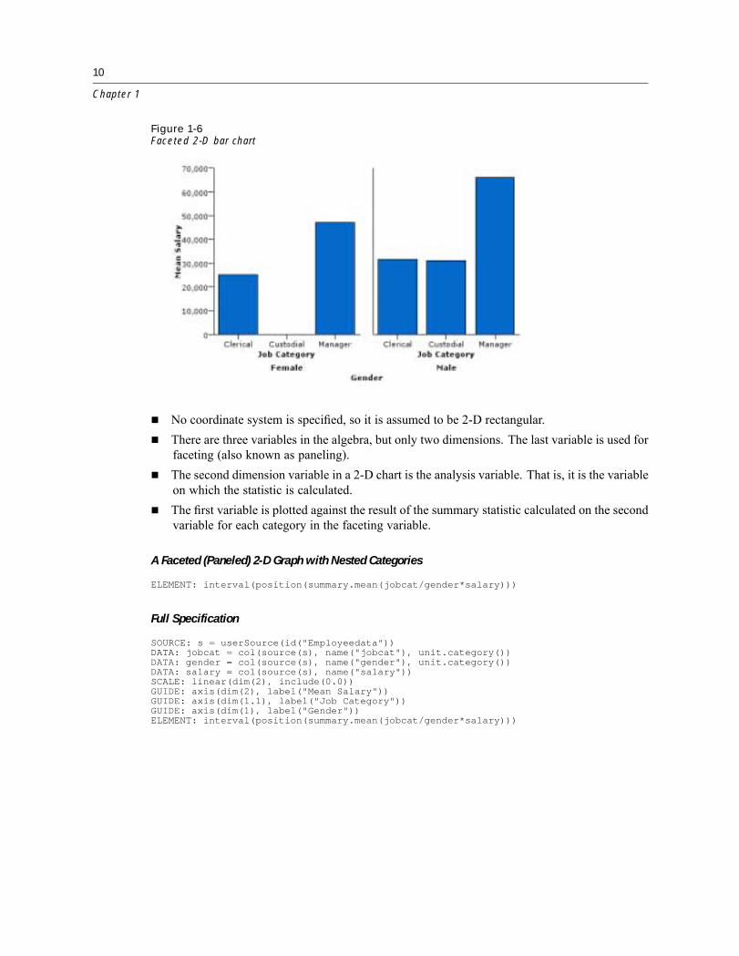
A Faceted (Paneled) 2-D Graph

ELEMENT: interval(position(summary.mean(jobcat*salary*gender)))

Full Specification

SOURCE: s = userSource(id("Employeedata"))DATA: jobcat = col(source(s), name("jobcat"), unit.category())DATA: gender = col(source(s), name("gender"), unit.category())DATA: salary = col(source(s), name("salary"))SCALE: linear(dim(2), include(0))GUIDE: axis(dim(3), label("Gender"))GUIDE: axis(dim(2), label("Mean Salary"))GUIDE: axis(dim(1), label("Job Category"))ELEMENT: interval(position(summary.mean(jobcat*salary*gender)))

10

Chapter 1

Figure 1-6Faceted 2-D bar chart

! No coordinate system is speciÞed, so it is assumed to be 2-D rectangular.! There are three variables in the algebra, but only two dimensions. The last variable is used for

faceting (also known as paneling).! The second dimension variable in a 2-D chart is the analysis variable. That is, it is the variable

on which the statistic is calculated.! The Þrst variable is plotted against the result of the summary statistic calculated on the second

variable for each category in the faceting variable.

A Faceted (Paneled) 2-D Graph with Nested Categories

ELEMENT: interval(position(summary.mean(jobcat/gender*salary)))

Full Specification

SOURCE: s = userSource(id("Employeedata"))DATA: jobcat = col(source(s), name("jobcat"), unit.category())DATA: gender = col(source(s), name("gender"), unit.category())DATA: salary = col(source(s), name("salary"))SCALE: linear(dim(2), include(0.0))GUIDE: axis(dim(2), label("Mean Salary"))GUIDE: axis(dim(1.1), label("Job Category"))GUIDE: axis(dim(1), label("Gender"))ELEMENT: interval(position(summary.mean(jobcat/gender*salary)))

11

Introduction to GPL

Figure 1-7Faceted 2-D bar chart with nested categories

! This example is the same as the previous paneled example, except for the algebra.! The second dimension variable is the same as in the previous example. Therefore, it is the

variable on which the statistic is calculated.! jobcat is nested in gender. Nesting always results in faceting, regardless of the available

dimensions.! With nested categories, only those combinations of categories that occur in the data are shown

in the graph. In this case, there is no bar for Female and Custodial in the graph, because thereis no case with this combination of categories in the data. Compare this result to the previousexample that created facets by crossing categorical variables.

A 3-D Graph

COORD: rect(dim(1,2,3))ELEMENT: interval(position(summary.mean(jobcat*gender*salary)))

Full Specification

SOURCE: s = userSource(id("Employeedata"))DATA: jobcat=col(source(s), name("jobcat"), unit.category())DATA: gender=col(source(s), name("gender"), unit.category())DATA: salary=col(source(s), name("salary"))COORD: rect(dim(1,2,3))SCALE: linear(dim(3), include(0))GUIDE: axis(dim(3), label("Mean Salary"))GUIDE: axis(dim(2), label("Gender"))GUIDE: axis(dim(1), label("Job Category"))ELEMENT: interval(position(summary.mean(jobcat*gender*salary)))

12

Chapter 1

Figure 1-83-D bar chart

! The coordinate system is explicitly set to three-dimensional, and there are three variablesin the algebra.

! The three variables are plotted on the available dimensions.! The third dimension variable in a 3-D chart is the analysis variable. This differs from the 2-D

chart in which the second dimension variable is the analysis variable.

A Clustered Graph

COORD: rect(dim(1,2), cluster(3))ELEMENT: interval(position(summary.mean(gender*salary*jobcat)), color(gender))

Full Specification

SOURCE: s = userSource(id("Employeedata"))DATA: jobcat=col(source(s), name("jobcat"), unit.category())DATA: gender=col(source(s), name("gender"), unit.category())DATA: salary=col(source(s), name("salary"))COORD: rect(dim(1,2), cluster(3))SCALE: linear(dim(2), include(0))GUIDE: axis(dim(2), label("Mean Salary"))GUIDE: axis(dim(3), label("Gender"))ELEMENT: interval(position(summary.mean(jobcat*salary*gender)), color(jobcat))

13

Introduction to GPL

Figure 1-9Clustered 2-D bar chart

! The coordinate system is explicitly set to two-dimensional, but it is modiÞed by the clusterfunction.

! The cluster function indicates that clustering occurs along dim(3), which is the dimensionassociated with jobcat because it is the third variable in the algebra.

! The variable in dim(1) identiÞes the variable whose values determine the bars in each cluster.This is gender.

! Although the coordinate system was modiÞed, this is still a 2-D chart. Therefore, the analysisvariable is still the second dimension variable.

! The variables are plotted using the modiÞed coordinate system. Note that the graph would bea paneled graph if you removed the cluster function. The charts would look similar andshow the same results, but their coordinate systems would differ. Refer back to the paneled2-D graph to see the difference.

Common Tasks

This section provides information for adding common graph features. This GPL creates asimple 2-D bar chart. You can apply the steps to any graph, but the examples use the GPL inThe Basics on p. 1 as a �baseline.�

How to Add Stacking to a Graph

Stacking involves a couple of changes to the ELEMENT statement. The following steps use theGPL shown in The Basics on p. 1 as a �baseline� for the changes.

14

Chapter 1

E Before modifying the ELEMENT statement, you need to deÞne an additional categorical variablethat will be used for stacking. This is speciÞed by a DATA statement (note the unit.category()function):

DATA: gender=col(source(s), name("gender"), unit.category())

E The Þrst change to the ELEMENT statement will split the graphic element into color groups foreach gender category. This splitting results from using the color function:

ELEMENT: interval(position(summary.mean(jobcat*salary)), color(gender))

E Because there is no collision modiÞer for the interval element, the groups of bars are overlaidon each other, and there�s no way to distinguish them. In fact, you may not even see graphicelements for one of the groups because the other graphic elements obscure them. You need to addthe stacking collision modiÞer to re-position the groups (we also changed the statistic becausestacking summed values makes more sense than stacking the mean values):

ELEMENT: interval.stack(position(summary.sum(jobcat*salary)), color(gender))

The complete GPL is shown below:

SOURCE: s = userSource(id("Employeedata"))DATA: jobcat = col(source(s), name("jobcat"), unit.category())DATA: gender = col(source(s), name("gender"), unit.category())DATA: salary = col(source(s), name("salary"))SCALE: linear(dim(2), include(0.0))GUIDE: axis(dim(2), label("Sum Salary"))GUIDE: axis(dim(1), label("Job Category"))ELEMENT: interval.stack(position(summary.sum(jobcat*salary)), color(gender))

Following is the graph created from the GPL.

Figure 1-10Stacked bar chart

15

Introduction to GPL

Legend Label

The graph includes a legend, but it has no label by default. To add or change the label for thelegend, you use a GUIDE statement:

GUIDE: legend(aesthetic(aesthetic.color), label("Gender"))

How to Add Faceting (Paneling) to a Graph

Faceted variables are added to the algebra in the ELEMENT statement. The following steps use theGPL shown in The Basics on p. 1 as a �baseline� for the changes.

E Before modifying the ELEMENT statement, we need to deÞne an additional categorical variablethat will be used for faceting. This is speciÞed by a DATA statement (note the unit.category()function):


E Now we add the variable to the algebra. We will cross the variable with the other variablesin the algebra:


Those are the only necessary steps. The Þnal GPL is shown below.

SOURCE: s = userSource(id("Employeedata"))DATA: jobcat = col(source(s), name("jobcat"), unit.category())DATA: gender = col(source(s), name("gender"), unit.category())DATA: salary = col(source(s), name("salary"))SCALE: linear(dim(2), include(0.0))GUIDE: axis(dim(2), label("Mean Salary"))GUIDE: axis(dim(1), label("Job Category"))ELEMENT: interval(position(summary.mean(jobcat*salary*gender)))


16

Chapter 1

Figure 1-11Faceted bar chart

Additional Features

Labeling. If you want to label the faceted dimension, you treat it like the other dimensions in thegraph by adding a GUIDE statement for its axis:

GUIDE: axis(dim(3), label("Gender"))

In this case, it is speciÞed as the 3rd dimension. You can determine the dimension number bycounting the crossed variables in the algebra. gender is the 3rd variable.

Nesting. Faceted variables can be nested as well as crossed. Unlike crossed variables, the nestedvariable is positioned next to the variable in which it is nested. So, to nest gender in jobcat,you would do the following:

ELEMENT: interval(position(summary.mean(jobcat/gender*salary)))

Because gender is used for nesting, it is not the 3rd dimension as it was when crossing to createfacets. You can�t use the same simple counting method to determine the dimension number.You still count the crossings, but you count each crossing as a single factor. The number thatyou obtain by counting each crossed factor is used for the nested variable (in this case, 1). Theother dimension is indicated by the nested variable dimension followed by a dot and the number1 (in this case, 1.1). So, you would use the following convention to refer to the gender andjobcat dimensions in the GUIDE statement:

GUIDE: axis(dim(1), label("Gender"))GUIDE: axis(dim(1.1), label("Job Category"))GUIDE: axis(dim(2), label("Mean Salary"))

17

Introduction to GPL

How to Add Clustering to a Graph

Clustering involves changes to the COORD statement and the ELEMENT statement. The followingsteps use the GPL shown in The Basics on p. 1 as a �baseline� for the changes.

E Before modifying the COORD and ELEMENT statements, you need to deÞne an additionalcategorical variable that will be used for clustering. This is speciÞed by a DATA statement (notethe unit.category() function):


E Now you will modify the COORD statement. If, like the baseline graph, the GPL does not alreadyinclude a COORD statement, you Þrst need to add one:

COORD: rect(dim(1,2))

In this case, the default coordinate system is now explicit.

E Next add the cluster function to the coordinate system and specify the clustering dimension. Ina 2-D coordinate system, this is the third dimension:

COORD: rect(dim(1,2), cluster(3))

E Now we add the clustering dimension variable to the algebra. This variable is in the 3rd position,corresponding to the clustering dimension speciÞed by the cluster function in the COORDstatement:


Note that this algebra looks similar to the algebra for faceting. Without the cluster functionadded in the previous step, the resulting graph would be faceted. The cluster functionessentially collapses the faceting into one axis. Instead of a facet for each gender category, thereis a cluster on the x axis for each category.

E Because clustering changes the dimensions, we update the GUIDE statement so that it correspondsto the clustering dimension.

GUIDE: axis(dim(3), label("Gender"))

E With these changes, the chart is clustered, but there is no way to distinguish the bars in eachcluster. You need to add an aesthetic to distinguish the bars:

ELEMENT: interval(position(summary.mean(jobcat*salary*gender)), color(jobcat))

The complete GPL looks like the following.


Following is the graph created from the GPL. Compare this to �Faceted bar chart� on p. 16.

18

Chapter 1

Figure 1-12Clustered bar chart

Legend Label

The graph includes a legend, but it has no label by default. To change the label for the legend,you use a GUIDE statement:


How to Use Aesthetics

GPL includes several different aesthetic functions for controlling the appearance of a graphicelement. The simplest use of an aesthetic function is to deÞne a uniform aesthetic for everyinstance of a graphic element. For example, you can use the color function to assign a colorconstant (like color.red) to the point element, thereby making all of the points in the graph red.A more interesting use of an aesthetic function is to change the value of the aesthetic based on

the value of another variable. For example, instead of a uniform color for the scatterplot points,the color could vary based on the value of the categorical variable gender. All of the points in theMale category will be one color, and all of the points in the Female category will be another.Using a categorical variable for an aesthetic creates groups of cases. In addition to identifying thegraphic elements for the groups of cases, the grouping allows you to evaluate statistics for theindividual groups, if needed.An aesthetic may also vary based on a set of continuous values. Using continuous values for

the aesthetic does not result in distinct groups of graphic elements. Instead, the aesthetic variesalong the same continuous scale. There are no distinct groups on the scale, so the color variesgradually, just as the continuous values do.The steps below use the following GPL as a �baseline� for adding the aesthetics. This GPL

creates a simple scatterplot.

19

Introduction to GPL

Figure 1-13Baseline GPL for example


E First, you need to deÞne an additional categorical variable that will be used for one of theaesthetics. This is speciÞed by a DATA statement (note the unit.category() function):


E Next you need to deÞne another variable, this one being continuous. It will be used for theother aesthetic.

DATA: prevexp=col(source(s), name("prevexp"))

E Now you will add the aesthetics to the graphic element in the ELEMENT statement. First add theaesthetic for the categorical variable:

ELEMENT: point(position(salbegin*salary), shape(gender))

Shape is a good aesthetic for the categorical variable. It has distinct values that correspondwell to categorical values.

E Finally add the aesthetic for the continuous variable:

ELEMENT: point(position(salbegin*salary), shape(gender), color(prevexp))

Not all aesthetics are available for continuous variables. That�s another reason why shape was agood aesthetic for the categorical variable. Shape is not available for continuous variables becausethere aren�t enough shapes to cover a continuous spectrum. On the other hand, color graduallychanges in the graph. It can capture the full spectrum of continuous values. Transparency orbrightness would also work well.

The complete GPL looks like the following.

SOURCE: s = userSource(id("Employeedata"))DATA: salbegin = col(source(s), name("salbegin"))DATA: salary = col(source(s), name("salary"))DATA: gender = col(source(s), name("gender"), unit.category())DATA: prevexp = col(source(s), name("prevexp"))GUIDE: axis(dim(2), label("Current Salary"))GUIDE: axis(dim(1), label("Beginning Salary"))ELEMENT: point(position(salbegin*salary), shape(gender), color(prevexp))


20

Chapter 1

Figure 1-14Scatterplot with aesthetics

Legend Label

The graph includes legends, but the legends have no labels by default. To change the labels, youuse GUIDE statements that reference each aesthetic:

GUIDE: legend(aesthetic(aesthetic.shape), label("Gender"))GUIDE: legend(aesthetic(aesthetic.color), label("Previous Experience"))

When interpreting the color legend in the example, it�s important to realize that the color aestheticcorresponds to a continuous variable. Only a handful of colors may be shown in the legend, andthese colors do not reßect the whole spectrum of colors that could appear in the graph itself. Theyare more like mileposts at major divisions.

What’s Changed in GPLIn addition to many new features, following are the important changes since the last release.These changes may affect GPL that you created previously.! References to nested dimensions now use a dot convention (for example, 1.1). For more

information, see dim Function in Chapter 2 on p. 102.! region.spread.confi was removed. Use region.confi.count,

region.confi.mean, or region.confi.percent instead.! Previously, you could use dim(1) in a GUIDE statement to refer to a clustered dimension.

This is incorrect. For general information about referring to dimensions, see dim Functionon p. 102. For an example of a clustered chart that uses the correct dimension reference,see Clustered Bar Chart on p. 223.

! If there are multiple ELEMENT statements in a single graph, you cannot use cumulativestatistics for some graphic elements but not for others. This behavior is prohibited because theresults of each statistic function would be blended on the same scale. The units for cumulative

21

Introduction to GPL

statistics do not match the units for non-cumulative statistics, so blending these results isimpossible. The exception is when the ELEMENT statements are linked to independent axes.

! GPL is now case sensitive. For more information, see Syntax Rules on p. 3.! summary.percent is now an alias for summary.percent.sum. If you want to calculate

a percentage based on count, use summary.percent.count(catVarName). The oldconvention, summary.percent(summary.count(catVarName)), is deprecated.

! The origin function for graphs is relative to top left corner instead of bottom left corneras it was previously. For more information, see origin Function (For Graphs) in Chapter 2on p. 152.

! The unit of measurement for binWidth defaults to seconds or days, depending on theunderlying format. Previously, the unit was always days. Include a qualiÞer to specify adifferent unit (for example, 30d). For more information, see binWidth Function in Chapter 2on p. 74.

Chapter

2222Statement and Function Reference

This section provides detailed information about the various statements that make up GPL and thefunctions that you can use in each of the statements.

StatementsThere are general categories of GPL statements.

Data definition statements. Data deÞnition statements specify the data sources, variables, andoptional variable transformations. All GPL code blocks include at least two data deÞnitionstatements: one to deÞne the actual data source and one to specify the variable extracted fromthe data source.

Specification statements. SpeciÞcation statements deÞne the graph. They deÞne the axis scales,coordinate systems, text, graphic elements (for example, bars and points), and statistics. AllGPL code blocks require at least one ELEMENT statement, but the other speciÞcation statementsare optional. GPL uses a default value when the SCALE, COORD, and GUIDE statements arenot included in the GPL code block.

Control statements. Control statements specify the layout for graphs. The GRAPH statementallows you to group multiple graphs in a single page display. For example, you may want to addhistograms to the borders on a scatterplot. The PAGE statement allows you to set the size of theoverall visualization. Control statements are optional.

Comment statement. The COMMENT statement is used for adding comments to the GPL. Theseare optional.

Data Definition Statements

SOURCE Statement, DATA Statement, TRANS Statement

Specification Statements

COORD Statement, SCALE Statement, GUIDE Statement, ELEMENT Statement

Control Statements

PAGE Statement, GRAPH Statement

Comment Statements

COMMENT Statement

22

23

Statement and Function Reference

COMMENT Statement

Syntax

COMMENT: <text>

<text>. The comment text. This can consist of any string of characters except a statement labelfollowed by a colon (:), unless the statement label and colon are enclosed in quotes (for example,COMMENT: With "SCALE:" statement).

Description

This statement is optional. You can use it to add comments to your GPL or to comment out astatement by converting it to a comment. The comment does not appear in the resulting graph.

Examples

Figure 2-1Defining a comment

COMMENT: This graph shows counts for each job category.

PAGE Statement

Syntax

PAGE: <function>

<function>. A function for specifying the PAGE statements that mark the beginning and endof the visualization.

Description

This statement is optional. It�s needed only when you specify a size for the page display orvisualization. The current release of GPL supports only one PAGE block.

Examples

Figure 2-2Example: Defining a page

PAGE: begin(scale(400px,300px))SOURCE: s=csvSource(file("mydata.csv"))DATA: x=col(source(s), name("x"))DATA: y=col(source(s), name("y"))ELEMENT: line(position(x*y))PAGE: end()

Figure 2-3Example: Defining a page with multiple graphs

PAGE: begin(scale(400px,300px))SOURCE: s=csvSource(file("mydata.csv"))DATA: a=col(source(s), name("a"))DATA: b=col(source(s), name("b"))DATA: c=col(source(s), name("c"))

24

Chapter 2

GRAPH: begin(scale(90%, 45%), origin(10%, 50%))ELEMENT: line(position(a*c))GRAPH: end()GRAPH: begin(scale(90%, 45%), origin(10%, 0%))ELEMENT: line(position(b*c))GRAPH: end()PAGE: end()

Valid Functions

begin Function (For Pages), end Function

GRAPH Statement

Syntax

GRAPH: <function>

<function>. A function for specifying the GRAPH statements that mark the beginning and end ofthe individual graph.

Description

This statement is optional. It�s needed only when you want to group multiple graphs in a singlepage display or you want to customize a graph�s size. The GRAPH statement is essentially awrapper around the GPL that deÞnes a particular graph. There is no limit to the number ofgraphs that can appear in a GPL block.Grouping graphs is useful for related graphs, like graphs on the borders of histograms.

However, the graphs do not have to be related. You may simply want to group the graphs forpresentation.

Examples

Figure 2-4Scaling a graph

GRAPH: begin(scale(50%,50%))

Figure 2-5Example: Scatterplot with border histograms

GRAPH: begin(origin(10.0%, 20.0%), scale(80.0%, 80.0%))ELEMENT: point(position(salbegin*salary))GRAPH: end()GRAPH: begin(origin(10.0%, 100.0%), scale(80.0%, 10.0%))ELEMENT: interval(position(summary.count(bin.rect(salbegin))))GRAPH: end()GRAPH: begin(origin(90.0%, 20.0%), scale(10.0%, 80.0%))COORD: transpose()ELEMENT: interval(position(summary.count(bin.rect(salary))))GRAPH: end()

Valid Functions

begin Function (For Graphs), end Function

25


SOURCE Statement

Syntax

SOURCE: <source name> = <function>

<source name>. User-deÞned name for the data source. Refer to Syntax Rules on p. 3 forinformation about which characters you can use in the name.

<function>. A function for extracting data from various data sources.

Description

DeÞnes a data source for the graph. There can be multiple data sources, each speciÞed by adifferent SOURCE statement.

Examples

Figure 2-6Example: Reading a CSV file

SOURCE: mydata = csvSource(path("C:\\Data\\demo.csv"))

Valid Functions

csvSource Function, mapSource Function, userSource Function

DATA Statement

Syntax

DATA: <variable name> = <function>

<variable name>. User-deÞned name for the variable. Refer to Syntax Rules on p. 3 forinformation about which characters you can use in the name.

<function>. A function indicating the data sources.

Description

DeÞnes a variable from a speciÞc data source. The GPL statement must also include a SOURCEstatement. The name identiÞed by the SOURCE statement is used in the DATA statement to indicatethe data source from which a particular variable is extracted.

Examples

Figure 2-7Example: Specifying a variable from a data source

DATA: age = col(source(mydata), name("age"))

26

Chapter 2

age is an arbitrary name. In this example, the variable name is the same as the name that appearsin the data source. Using the same name avoids confusion. The col function takes a data sourceand data source variable name as its arguments. Note that the data source name was previouslydeÞned by a SOURCE statement and is not enclosed in quotes.

Valid Functions

col Function, iter Function, mapVariables Function

TRANS Statement

Syntax

TRANS: <variable name> = <function>

<variable name>. A string that speciÞes a name for the variable that is created as a result ofthe transformation. Refer to Syntax Rules on p. 3 for information about which characters youcan use in the name.

<function>. A valid function.

Description

DeÞnes a new variable whose value is the result of a data transformation function.

Examples

Figure 2-8Example: Creating a transformation variable from other variables

TRANS: saldiff = eval(((salary-salbegin)/salary)*100)

Figure 2-9Example: Creating an index variable

TRANS: casenum = index()

Valid Functions

collapse Function, eval Function, index Function

COORD Statement

Syntax

COORD: <coord>

<coord>. A valid coordinate type or transformation function.

27


Description

SpeciÞes a coordinate system for the graph. You can also embed coordinate systems or wrapa coordinate system in a transformation. When transformations and coordinate systems areembedded in each other, they are applied in order, with the innermost being applied Þrst. Thus,mirror(transpose(rect(1,2))) speciÞes that a 2-D rectangular coordinate system istransposed and then mirrored.

Examples

Figure 2-10Example: Polar coordinates for pie charts

COORD: polar.theta()

Figure 2-11Example: 3-D rectangular coordinates

COORD: rect(dim(1,2,3))

Figure 2-12Example: Embedded coordinate systems for paneled pie chart

COORD: rect(dim(2), polar.theta(dim(1)))

Figure 2-13Example: Transposed coordinate system

COORD: transpose()

Coordinate Types and Transformations

parallel Coordinate Type, polar Coordinate Type, polar.theta Coordinate Type, rect CoordinateType, mirror Function, project Function, reßect Function, transpose Function, wrap Function

Coordinate Types

There are several coordinate types available in GPL.

Coordinate Types

parallel Coordinate Type, polar Coordinate Type, polar.theta Coordinate Type, rect CoordinateType

parallel Coordinate Type

Syntax

parallel(dim(<numeric>), <coord>)

<numeric>. One or more numeric values (separated by commas) indicating the graph dimensionor dimensions to which the parallel coordinate system applies. The number of values equals thenumber of dimensions for the coordinate system�s frame, and the values are always in sequentialorder. For example, parallel(dim(1,2,3,4)) indicates that the Þrst four variables in the

28

Chapter 2

algebra are used for the parallel coordinates. Any others are used for faceting. If no dimensionsare speciÞed, all variables are used for the parallel coordinates. For more information, see dimFunction on p. 102.

<coord>. A valid coordinate type or transformation function. This is optional.

Description

Creates a parallel coordinate system. A graph using this coordinate system consists of multiple,parallel axes showing data across multiple variables, resulting in a plot that is similar to a proÞleplot.When you use a parallel coordinate system, you cross each continuous variable in the algebra.

A line graphic element is the most common element type for this graph. The graphic element isalways distinguished by some aesthetic so that any patterns are readily apparent.

Examples

Figure 2-14Example: Parallel coordinates graph

TRANS: caseid = index()COORD: parallel()ELEMENT: line(position(var1*var2*var3*var4), split(caseid), color(catvar1))

The example includes the split function to create a separate line for each case in the data.Otherwise, there would be only one line that crossed back through the coordinate system toconnect all the cases.


polar Coordinate Type, polar.theta Coordinate Type, rect Coordinate Type, mirror Function,project Function, reßect Function, transpose Function, wrap Function

Applies To

COORD Statement, polar Coordinate Type, polar.theta Coordinate Type, rect Coordinate Type,project Function

polar Coordinate Type

Syntax

polar(dim(<numeric>), <function>, <coord>)

<numeric>. Numeric values (separated by commas) indicating the dimensions to which thepolar coordinates apply. This is optional and is assumed to be the Þrst two dimensions. Formore information, see dim Function on p. 102.

<function>. One or more valid functions. These are optional.


29


Description

Creates a polar coordinate system. This differs from the polar.theta coordinate system in thatit is two dimensional. One dimension is associated with the radius, and the other is associatedwith the theta angle.

Examples

Figure 2-15Example: Polar line chart

COORD: polar()ELEMENT: line(position(date*close), closed(), preserveStraightLines())

Valid Functions

reverse Function, startAngle Function


parallel Coordinate Type, polar.theta Coordinate Type, rect Coordinate Type, mirror Function,project Function, reßect Function, transpose Function, wrap Function

Applies To

COORD Statement, parallel Coordinate Type, polar.theta Coordinate Type, rect CoordinateType, project Function

polar.theta Coordinate Type

Syntax

polar.theta(<function>, <coord>)

<numeric>. A numeric value indicating the dimension. This is optional and required only whenpolar.theta is not the Þrst or innermost dimension. Otherwise, it is assumed to be the Þrstdimension. For more information, see dim Function on p. 102.



Description

Creates a polar.theta coordinate system, which is the coordinate system for creating pie charts.polar.theta differs from the polar coordinate system in that it is one dimensional. This is thedimension for the theta angle.

30

Chapter 2

Examples

Figure 2-16Example: Pie chart

COORD: polar.theta()ELEMENT: interval.stack(position(summary.count()), color(jobcat))

Valid Functions

reverse Function, startAngle Function


parallel Coordinate Type, polar Coordinate Type, rect Coordinate Type, mirror Function, projectFunction, reßect Function, transpose Function, wrap Function

Applies To

COORD Statement, parallel Coordinate Type, polar Coordinate Type, rect Coordinate Type,project Function

rect Coordinate Type

Syntax

rect(dim(<numeric>), <function>, <coord>)

<numeric>. One or more numeric values (separated by commas) indicating the graph dimensionor dimensions to which the rectangular coordinate system applies. The number of values equalsthe number of dimensions for the coordinate system�s frame, and the values are always insequential order (for example, dim(1,2,3) and dim(4,5)). For more information, see dimFunction on p. 102.



Description

Creates a rectangular coordinate system. By default, a rectangular coordinate system is 2-D,which is the equivalent of specifying rect(dim(1,2)). To create a 3-D coordinate system,use rect(dim(1,2,3)). Similarly, use rect(dim(1)) to specify a 1-D coordinate system.Changing the coordinate system also changes which variable in the algebra is summarized for astatistic. The statistic function is calculated on the second crossed variable in a 2-D coordinatesystem and the third crossed variable in a 3-D coordinate system.

Examples

Figure 2-17Example: 2-D bar chart

COORD: rect(dim(1,2))ELEMENT: interval(position(summary.mean(jobcat*salary)))

31


Figure 2-18Example: 3-D bar chart

COORD: rect(dim(1,2,3))ELEMENT: interval(position(summary.mean(jobcat*gender*salary)))

Valid Functions

cluster Function, sameRatio Function


parallel Coordinate Type, polar Coordinate Type, polar.theta Coordinate Type, mirror Function,project Function, reßect Function, transpose Function, wrap Function

Applies To

COORD Statement, parallel Coordinate Type, polar Coordinate Type, polar.theta CoordinateType, project Function

SCALE Statement

Syntax

SCALE: <scale type>

or

SCALE: <scale name> = <scale type>

<scale type>. A valid scale type.

<scale name>. A user-deÞned name for the scale. This is required only when you are creating agraph with dual scales. An example is a graph that shows the mean of a variable on one axis andthe count on the other. The scale name is referenced by an axis and a graphic element to indicatewhich scale is associated with the axis and graphic element. Refer to Syntax Rules on p. 3 forinformation about which characters you can use in the name.

Description

DeÞnes the scale for a particular dimension or aesthetic (such as color).

Examples

Figure 2-19Example: Specifying a linear dimension scale

SCALE: linear(dim(2), max(50000))

Figure 2-20Example: Specifying a log aesthetic scale

SCALE: log(aesthetic(aesthetic.color))ELEMENT: point(position(x*y), color(z))

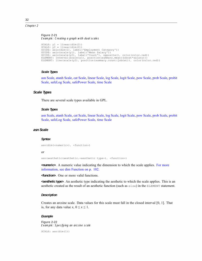
32

Chapter 2

Figure 2-21Example: Creating a graph with dual scales

SCALE: y1 = linear(dim(2))SCALE: y2 = linear(dim(2))GUIDE: axis(dim(1), label("Employment Category"))GUIDE: axis(scale(y1), label("Mean Salary"))GUIDE: axis(scale(y2), label("Count"), opposite(), color(color.red))ELEMENT: interval(scale(y1), position(summary.mean(jobcat*salary)))ELEMENT: line(scale(y2), position(summary.count(jobcat)), color(color.red))

Scale Types

asn Scale, atanh Scale, cat Scale, linear Scale, log Scale, logit Scale, pow Scale, prob Scale, probitScale, safeLog Scale, safePower Scale, time Scale

Scale Types

There are several scale types available in GPL.

Scale Types


asn Scale

Syntax

asn(dim(<numeric>), <function>)

or

asn(aesthetic(aesthetic.<aesthetic type>), <function>)

<numeric>. A numeric value indicating the dimension to which the scale applies. For moreinformation, see dim Function on p. 102.

<function>. One or more valid functions.

<aesthetic type>. An aesthetic type indicating the aesthetic to which the scale applies. This is anaesthetic created as the result of an aesthetic function (such as size) in the ELEMENT statement.

Description

Creates an arcsine scale. Data values for this scale must fall in the closed interval [0, 1]. Thatis, for any data value x, 0 ≤ x ≤ 1.

Example

Figure 2-22Example: Specifying an arcsine scale

SCALE: asn(dim(1))

33


Valid Functions

aestheticMaximum Function, aestheticMinimum Function, aestheticMissing Function

Applies To

SCALE Statement

atanh Scale

Syntax

atanh(dim(<numeric>), <function>)

or

atanh(aesthetic(aesthetic.<aesthetic type>), <function>)




Description

Creates a Fisher�s z scale (also called the hyberbolic arctangent scale). Data values for this scalemust fall in the open interval (-1, 1). That is, for any data value x, -1 < x < 1.

Example

Figure 2-23Example: Specifying a Fisher’s z scale

SCALE: atanh(dim(1))

Applies To

SCALE Statement

Valid Functions


cat Scale

Syntax

cat(dim(<numeric>), <function>)

or

34

Chapter 2

cat(aesthetic(aesthetic.<aesthetic type>), <function>)



<aesthetic type>. An aesthetic type indicating the aesthetic to which the scale applies. This is anaesthetic created as the result of an aesthetic function in the ELEMENT statement, often used fordistinguishing groups of graphic elements, as in clusters and stacks.

Description

Creates a categorical scale that can be associated with a dimension (such as an axis or panelfacet) or an aesthetic (as in the legend). A categorical scale is created for a categorical variableby default. You usually don�t need to specify the scale unless you want to use a function tomodify it (for example, to sort the categories).

Examples

Figure 2-24Example: Specifying the scale for a dimension and sorting categories

SCALE: cat(dim(1), sort.natural())

Figure 2-25Example: Specifying the scale for an aesthetic and including categories

SCALE: cat(aesthetic(aesthetic.color), include("IL"))

Note: The exclude function is not supported for aesthetic scales.

Applies To

SCALE Statement

Valid Functions

aestheticMissing Function, values Function, exclude Function, include Function, map Function,reverse Function, sort.data Function, sort.natural Function, sort.statistic Function, sort.valuesFunction

linear Scale

Syntax

linear(dim(<numeric>), <function>)

or

linear(aesthetic(aesthetic.<aesthetic type>), <function>)


35




Description

Creates a linear scale. A linear scale is created for a continuous variable by default. You usuallydon�t need to specify the scale unless you want to add a function to modify it (for example,to specify the range).

Example

Figure 2-26Example: Specifying a maximum value for the linear scale


Applies To

SCALE Statement

Valid Functions

aestheticMaximum Function, aestheticMinimum Function, aestheticMissing Function,dataMaximum Function, dataMinimum Function, include Function, max Function, min Function,origin Function (For Scales), reverse Function

log Scale

Syntax

log(dim(<numeric>), <function>)

or

log(aesthetic(aesthetic.<aesthetic type>), <function>)




Description

Creates a logarithmic scale. If a base is not explicitly speciÞed, the default is base 10. Datavalues for this scale must be greater than 0.

36

Chapter 2

Example

Figure 2-27Example: Specifying the scale and a base

SCALE: log(dim(2), base(2))

Applies To

SCALE Statement

Valid Functions

aestheticMaximum Function, aestheticMinimum Function, aestheticMissing Function,dataMaximum Function, dataMinimum Function, include Function, base Function, max Function,min Function, origin Function (For Scales), reverse Function

logit Scale

Syntax

logit(dim(<numeric>), <function>)

or

logit(aesthetic(aesthetic.<aesthetic type>), <function>)




Description

Creates a logit scale. Data values for this scale must fall in the open interval (0, 1). That is, forany data value x, 0 < x < 1.

Example

Figure 2-28Example: Specifying a logit scale

SCALE: logit(dim(2))

Applies To

SCALE Statement

Valid Functions


37


pow Scale

Syntax

pow(dim(<numeric>), <function>)

or

pow(aesthetic(aesthetic.<aesthetic type>), <function>)




Description

Creates a power scale. If an exponent is not explicitly speciÞed, the default is 0.5.

Example

Figure 2-29Example: Specifying the scale and an exponent

SCALE: pow(dim(2), exponent(2))

Applies To

SCALE Statement

Valid Functions

aestheticMaximum Function, aestheticMinimum Function, aestheticMissing Function,dataMaximum Function, dataMinimum Function, exponent Function, include Function, maxFunction, min Function, origin Function (For Scales), reverse Function

prob Scale

Syntax

prob(dim(<numeric>), <distribution function>, <function>)

or

prob(aesthetic(aesthetic.<aesthetic type>), <distribution function>, <function>)


<distribution function>. A distribution function. This is required.


38

Chapter 2


Description

Creates a probability scale based on a probability distribution. Data values for this scale must fallin the open interval (0, 1). That is, for any data value x, 0 < x < 1.

Example

Figure 2-30Example: Specifying a beta distribution for the probability scale

SCALE: prob(dim(2), beta(2, 5))

Applies To

SCALE Statement

Distribution Functions

beta Function, chiSquare Function, exponential Function, f Function, gamma Function, logisticFunction, normal Function, poisson Function, studentizedRange Function, t Function, uniformFunction, weibull Function

Valid Functions


probit Scale

Syntax

probit(dim(<numeric>), <function>)

or

probit(aesthetic(aesthetic.<aesthetic type>), <function>)




Description

Creates a probit scale. Data values for this scale must fall in the closed interval [0, 1]. Thatis, for any data value x, 0 ≤ x ≤ 1.

39


Example

Figure 2-31Example: Specifying a probit scale

probit(dim(2))

Applies To

SCALE Statement

Valid Functions


safeLog Scale

Syntax

safeLog(dim(<numeric>), <function>)

orsafeLog(aesthetic(aesthetic.<aesthetic type>), <function>)




Description

Creates a �safe� logarithmic scale. Unlike a regular log scale, the safe log scale uses a modiÞedfunction to handle 0 and negative values. If a base is not explicitly speciÞed, the default is base 10.

The safe log formula is:

sign(x) * log(1 + abs(x))

So if you assume that the axis value is �99, the result of the transformation is:

sign(-99) * log(1 + abs(-99)) = -1 * log(1 + 99) = -1 * 2 = -2

Example

Figure 2-32Example: Specifying the scale and a base

SCALE: safeLog(dim(2), base(2))

Applies To

SCALE Statement

40

Chapter 2

Valid Functions

aestheticMaximum Function, aestheticMinimum Function, aestheticMissing Function,dataMaximum Function, dataMinimum Function, include Function, base Function, max Function,min Function, origin Function (For Scales), reverse Function

safePower Scale

Syntax

safePower(dim(<numeric>), <function>)

or

safePower(aesthetic(aesthetic.<aesthetic type>), <function>)




Description

Creates a �safe� power scale. Unlike a regular power scale, the safe power scale uses a modiÞedfunction to handle negative values. If an exponent is not explicitly speciÞed, the default is 0.5.

When the exponent is a positive number, the safe power formulas are:

If (x>=0):pow(1+x, exponent)-1If (x<0):1-pow(1-x, exponent)

When the exponent is a negative number, the safe power formulas are:

If (x>=0):1-pow(1+x, exponent)If (x<0):pow(1-x, exponent)-1

So, if you assume the axis value is �99 and the exponent is 0.5, the result of the transformation is:

1 - pow(1 - (-99), 0.5) = 1 - pow(100, 0.5) = 1 - 10 = -9

So, if you assume the axis value is �99 and the exponent is �2, the result of the transformation is:

pow(1 - (-99), -2) - 1 = pow(100, -2) - 1 = 0.0001 - 1 = -0.999

Example

Figure 2-33Example: Specifying the scale and an exponent

SCALE: safePower(dim(2), exponent(10))

41


Applies To

SCALE Statement

Valid Functions

aestheticMaximum Function, aestheticMinimum Function, aestheticMissing Function,dataMaximum Function, dataMinimum Function, exponent Function, include Function, maxFunction, min Function, origin Function (For Scales), reverse Function

time Scale

Syntax

time(dim(<numeric>), <function>)

or

time(aesthetic(aesthetic.<aesthetic type>), <function>)




Description

Creates a time scale.

Example

Figure 2-34Example: Specifying a maximum value for the time scale

SCALE: time(dim(1), max("12/31/2005"))

Applies To

SCALE Statement

Valid Functions

aestheticMaximum Function, aestheticMinimum Function, aestheticMissing Function,dataMaximum Function, dataMinimum Function, include Function, max Function, min Function,origin Function (For Scales), reverse Function

42

Chapter 2

GUIDE Statement

Syntax

GUIDE: <guide type>

<guide type>. A valid guide type.

Description

SpeciÞes a guide for the graph. Guides provide additional information that can help a viewerinterpret the graph. An axis is a guide because it provides labels for the categories and values in agraph (but is separate from the scale on which the data are drawn). A title is a guide because itdescribes the graph. A legend is a guide because it provides color swatches to match a categoryname to speciÞc instances of a graphic element in the graph.

Examples

Figure 2-35Example: Axis

GUIDE: axis(dim(2), label("Mean Current Salary"))

Guide Types

axis Guide Type, legend Guide Type, text.footnote Guide Type, text.subfootnote Guide Type,text.subsubfootnote Guide Type, text.subtitle Guide Type, text.title Guide Type

Guide Types

There are several different types of guides.

Guide Types


axis Guide Type

Syntax

axis(dim(<numeric>), <function>)

or

axis(scale(<scale name>), <function>)


<function>. One or more valid functions. Use the null() function to hide the axis.

43


<scale name>. The name of the scale to which the axis applies. For more information, see scaleFunction (For Axes) on p. 169.

Description

SpeciÞes the axis for a particular dimension. Do not confuse the axis with the scale. They areseparate parts of the graph and are handled with separate GPL statements. The axis helpsinterpret the scale with labels and tick marks, but the axis does not change the positioningof graphic elements as changing the scale would. For information about scales, see SCALEStatement on p. 31.

Examples

Figure 2-36Example: Specifying an axis label for a dimension with one scale

GUIDE: axis(dim(2), label("Mean Current Salary"))

Figure 2-37Example: Specifying axis labels for a dimension with two scales

SCALE: y1 = linear(dim(2))SCALE: y2 = linear(dim(2))GUIDE: axis(scale(y1), label("Mean Salary"))GUIDE: axis(scale(y2), label("Count"), opposite(), color(color.red))

Applies To

GUIDE Statement

Valid Functions

color Function (For Axes), delta Function, gap Function, gridlines Function, label Function (ForGuides), opposite Function, unit.percent Function, start Function, ticks Function

legend Guide Type

Syntax

legend(aesthetic(aesthetic.<aesthetic type>), <function>)

<aesthetic type>. An aesthetic associated with the legend. The aesthetic identiÞes the legend,which was created as the result of an aesthetic function in the ELEMENT statement.

<function>. One or more valid functions. Use the null() function to hide the legend.

Description

SpeciÞes properties of the legend associated with a speciÞc aesthetic, which is deÞned by anaesthetic function in the ELEMENT statement. The legend provides a visual representation of thescale created by the aesthetic function. Thus, a legend guide is related to the aesthetic scale inthe same way an axis guide is related to a dimension scale. Note that using a uniform aesthetic

44

Chapter 2

value in the aesthetic function (for example, color(color.blue)) does not create a scale.Therefore, the legend is not used in that case.

Examples

Figure 2-38Example: Specifying a legend title

GUIDE: legend(aesthetic(aesthetic.color), label("Gender"))ELEMENT: interval(position(summary.count(jobcat)), color(gender))

Applies To

GUIDE Statement

Valid Functions

label Function (For Guides)

text.footnote Guide Type

Syntax

text.footnote(<function>)


Description

SpeciÞes the footnote for the graph.

Examples

Figure 2-39Example: Specifying the footnote text

GUIDE: text.footnote(label("Some Text"))

Applies To

GUIDE Statement

Valid Functions


text.subfootnote Guide Type

Syntax

text.subfootnote(<function>)


45


Description

SpeciÞes the second-level footnote for the graph. That is, the subfootnote appears below thefootnote.

Examples

Figure 2-40Example: Specifying the second-level footnote text

GUIDE: text.subfootnote(label("Some Text"))

Applies To

GUIDE Statement

Valid Functions


text.subsubfootnote Guide Type

Syntax

text.subsubfootnote(<function>)


Description

SpeciÞes the third-level footnote for the graph. That is, the subsubfootnote appears below thesubfootnote.

Examples

Figure 2-41Example: Specifying the third-level footnote text

GUIDE: text.subsubfootnote(label("Some Text"))

Applies To

GUIDE Statement

Valid Functions


text.subtitle Guide Type

Syntax

text.subtitle(<function>)

46

Chapter 2


Description

SpeciÞes the subtitle for the graph.

Examples

Figure 2-42Example: Specifying the subtitle text

GUIDE: text.subtitle(label("Some Text"))

Applies To

GUIDE Statement

Valid Functions


text.title Guide Type

Syntax

text.title(<function>)


Description

SpeciÞes the title for the graph.

Examples

Figure 2-43Example: Specifying the title text

GUIDE: text.title(label("Salary by Gender"))

Applies To

GUIDE Statement

Valid Functions


47


ELEMENT Statement

Syntax

ELEMENT: <element type>

<element type>. A valid element type.

Description

SpeciÞes a graphic element used to draw data on the graph. Graphic elements are the bars,points, lines, etc., that make up a graph.There can be multiple ELEMENT statements in the same block of GPL to create multiple

graphic elements. In this case, the variables in multiple ELEMENT statements share the samedimension and aesthetic scales.

For example, assume the GPL includes the following ELEMENT statements:

ELEMENT: point(position(x*y))ELEMENT: point(position(x2*y2))

In the resulting graph, dimension 1 uses x+x2, and dimension 2 uses y+y2.

Note: This behavior is sometimes called an implied blend because we could have written theGPL as follows:

ELEMENT: point(position(x*y+x2*y2))

Examples

Figure 2-44Example: Scatterplot

ELEMENT: point(position(x*y))

Figure 2-45Example: Line chart

ELEMENT: line(position(x*y))

Figure 2-46Example: Bar chart of means

ELEMENT: interval(position(summary.mean(x*y)))

Graphic Element Types

area Element, edge Element, interval Element, line Element, path Element, point Element,polygon Element, schema Element

Graphic Element Types

There are several different types of elements for drawing data on a graph.

48

Chapter 2

area Element

Syntax

area.<collision modifier>(<function>)

<collision modifier>. A method that speciÞes what should happen when two area graphic elementsoverlap each other. The collision modiÞer is optional.

<function>. One or more valid functions. The position function is required. The scalefunction is required when there are multiple scales in a single dimension (as in a �dual axis�graph).

Description

SpeciÞes an area graphic element.

Examples

Figure 2-47Example: Area chart

ELEMENT: area(position(summary.mean(jobcat*gender)))

Collision Modifiers

difference Collision ModiÞer, stack Collision ModiÞer

Valid Functions

color.brightness Function, closed Function, color Function (For Graphic Elements), color.hueFunction, jump Function, label Function (For Graphic Elements), missing.gap Function,missing.interpolate Function, missing.wings Function, texture.pattern Function, positionFunction, preserveStraightLines Function, color.saturation Function, scale Function (For GraphicElements), split Function, transparency Function

Applies To

ELEMENT Statement

bar Element

Description

bar is an alias for interval. For the syntax and other examples, see interval Element on p. 49.

Examples

Figure 2-48Example: Bar chart

ELEMENT: bar(position(summary.mean(jobcat*gender)))

49


edge Element

Syntax

edge(<function>)


Description

SpeciÞes a vertex-edge graphic element. The edge element is typically used in conjunction with alink or layout function, which calculates the actual links among the vertices. The edge elementis a graphical representation of these links.

Examples

Figure 2-49Example: Minimum spanning tree

ELEMENT: edge(position(link.mst(x*y))

Figure 2-50Example: Convex hull

ELEMENT: edge(position(link.hull(x*y))

Valid Functions

color.brightness Function, closed Function, color Function (For Graphic Elements), color.hueFunction, label Function (For Graphic Elements), missing.gap Function, missing.interpolateFunction, missing.wings Function, position Function, preserveStraightLines Function,color.saturation Function, scale Function (For Graphic Elements), shape Function, size Function,split Function, transparency Function

Applies To

ELEMENT Statement

interval Element

Syntax

interval.<collision modifier>(<function>)

<collision modifier>. A method that speciÞes what should happen when two interval graphicelements overlap each other. The collision modiÞer is optional.


50

Chapter 2

Description

SpeciÞes an interval (bar) graphic element, as would be used in a bar chart, histogram, or errorbar chart.

Examples

Figure 2-51Example: Bar chart

ELEMENT: interval(position(summary.mean(jobcat*salary)))

Figure 2-52Example: Histogram

ELEMENT: interval(position(bin.rect(summary.count(salary))))

Figure 2-53Example: Error bar chart

ELEMENT: interval(position(region.confi.mean(jobcat*salary)), shape(shape.ibeam))

Figure 2-54Example: Stacked bar chart

ELEMENT: interval.stack(position(summary.sum(jobcat*salary)), color(gender))

Collision Modifiers

dodge Collision ModiÞer, stack Collision ModiÞer

Valid Functions

color.brightness Function, color Function (For Graphic Elements), color.hue Function, labelFunction (For Graphic Elements), texture.pattern Function, position Function, color.saturationFunction, scale Function (For Graphic Elements), shape Function, size Function, split Function,transparency Function

Applies To

ELEMENT Statement

line Element

Syntax

line.<collision modifier>(<function>)

<collision modifier>. A method that speciÞes what should happen when two line graphic elementsoverlap each other. The collision modiÞer is optional.


51


Description

SpeciÞes a line graphic element. The line is drawn through values in the order in which theyappear in the x-axis domain. This is one of the features that distinguishes a line graphic elementfrom the path graphic element. See path Element on p. 51 for more information about the pathgraphic element.

Examples

Figure 2-55Example: Line chart of continuous variables

ELEMENT: line(position(salbegin*salary))

Figure 2-56Example: Line chart of a summary statistic

ELEMENT: line(position(summary.mean(jobcat*salary)))

Collision Modifiers

stack Collision ModiÞer

Valid Functions

color.brightness Function, closed Function, color Function (For Graphic Elements), color.hueFunction, jump Function, label Function (For Graphic Elements), missing.gap Function,missing.interpolate Function, missing.wings Function, position Function, preserveStraightLinesFunction, color.saturation Function, scale Function (For Graphic Elements), shape Function, sizeFunction, split Function, transparency Function

Applies To

ELEMENT Statement

path Element

Syntax

path(<function>)


Description

SpeciÞes a path graphic element. The path graphic element connects the data values in the orderin which their associated cases appear in the dataset. Therefore, it can cross back on itself. Thisis one of the features that distinguishes the path graphic element from the line graphic element.Additionally, paths can have variable sizes, so another variable can control the thickness of thepath at any particular point.

52

Chapter 2

Examples

Figure 2-57Example: Line chart drawn through all values

ELEMENT: path(position(salbegin*salary))

Figure 2-58Example: Creating a line chart with variable widths

ELEMENT: path(position(salbegin*salary), size(educ))

Valid Functions

color.brightness Function, closed Function, color Function (For Graphic Elements), color.hueFunction, label Function (For Graphic Elements), missing.gap Function, missing.interpolateFunction, missing.wings Function, position Function, preserveStraightLines Function,color.saturation Function, scale Function (For Graphic Elements), shape Function, size Function,split Function, transparency Function

Applies To

ELEMENT Statement

point Element

Syntax

point.<collision modifier>(<function>)

<collision modifier>. A method that speciÞes what should happen when two points overlap eachother. The collision modiÞer is optional.


Description

SpeciÞes a point graphic element, as would be used in a scatterplot.

Examples


ELEMENT: point(position(salbegin*salary))

Figure 2-60Example: Dot plot

ELEMENT: point.dodge.symmetric(position(bin.dot(salary)))

53


Collision Modifiers

dodge.asymmetric Collision ModiÞer, dodge.symmetric Collision ModiÞer, jitter CollisionModiÞer, stack Collision ModiÞer

Valid Functions

color.brightness Function, color Function (For Graphic Elements), color.hue Function, labelFunction (For Graphic Elements), texture.pattern Function, position Function, color.saturationFunction, scale Function (For Graphic Elements), shape Function, size Function, split Function,transparency Function

Applies To

ELEMENT Statement

polygon Element

Syntax

polygon(<function>)


Description

SpeciÞes a polygonal graphic element. A polygon connects multiple points to create an enclosedspace. For example, it may be used to draw a state or country in a map, or it may be used todraw the outline of a two-dimensional bin.

Examples

Figure 2-61Example: Hexagonal binning

ELEMENT: polygon(position(bin.hex(x*y, dim(1,2)), color(summary.count()))

Valid Functions

color.brightness Function, color Function (For Graphic Elements), color.hue Function,label Function (For Graphic Elements), position Function, preserveStraightLines Function,color.saturation Function, scale Function (For Graphic Elements), shape Function, size Function,split Function, transparency Function

Applies To

ELEMENT Statement

54

Chapter 2

schema Element

Syntax

schema(<function>)


Description

SpeciÞes a schema (boxplot) graphic element.

Examples

Figure 2-62Example: Boxplot

ELEMENT: schema(position(bin.quantile.letter(jobcat*salary)))

Valid Functions

color.brightness Function, color Function (For Graphic Elements), color.hue Function, labelFunction (For Graphic Elements), texture.pattern Function, position Function, color.saturationFunction, scale Function (For Graphic Elements), size Function, split Function, transparencyFunction

Applies To

ELEMENT Statement

Collision Modifiers

Collision modiÞers specify what happens when two graphic elements overlap.

difference Collision Modifier

Syntax

<element type>.difference


Description

Clips graphic elements and draws the difference between dichotomous values. The aestheticvalue associated with the greater value in a group determines the aesthetic for the result. Thisfunction is used to create a difference area graph. It is useful to compare the result to the oneobtained when using the stack position modiÞer.

55


Examples

Figure 2-63Example: Difference area chart

ELEMENT: area.difference(position(summary.sum(jobcat*salary)), color(gender))

Valid Element Types

area Element

dodge Collision Modifier

Syntax

<element type>.dodge


Description

Moves graphic elements next to other graphic elements that appear at the same value, rather thansuperimposing them. The graphic elements are arranged symmetrically. That is, the graphicelements are moved to opposite sides of a central position. For point elements, this function is thesame as dodge.symmetric. (See dodge.symmetric Collision ModiÞer on p. 56.)Although dodged charts can look similar to clustered charts, they are not the same. Clustering

changes the coordinates. Dodging only repositions graphic elements to avoid collisions.Therefore, a clustered chart allocates space for missing categories while a dodged chart does not.

Examples

Figure 2-64Example: 2-D Dot plot

ELEMENT: point.dodge(position(bin.dot(salary*jobcat)))

Figure 2-65Example: Dodged bar chart

ELEMENT: interval.dodge(position(summary.mean(jobcat*salary)), color(gender))

Valid Element Types

interval Element, point Element

dodge.asymmetric Collision Modifier

Syntax

<element type>.dodge.asymmetric


56

Chapter 2

Description

Moves graphic elements next to other graphic elements that appear at the same value, rather thansuperimposing them. The graphic elements are arranged asymmetrically. That is, the graphicelements are stacked on top of one another, with the graphic element on the bottom positioned ata speciÞc value on the scale. dodge.asymmetric is typically used for 1-D dot plots.

Examples


ELEMENT: point.dodge.asymmetric(position(bin.dot(salary)))

Valid Element Types

point Element

dodge.symmetric Collision Modifier

Syntax

<element type>.dodge.symmetric


Description

Moves graphic elements next to other graphic elements that appear at the same value, rather thansuperimposing them. The graphic elements are arranged symmetrically. That is, the graphicelements extend in two directions from a central position. dodge.asymmetric is typicallyused for 2-D dot plots.

Examples


ELEMENT: point.dodge.symmetric(position(bin.dot(salary*jobcat)))

Valid Element Types

point Element

jitter Collision Modifier

Syntax

<element type>.jitter.<jitter type>


57


<jitter type>. A valid jitter type. This is optional. If no type is speciÞed, jitter.joint.uniformis used.

Description

Repositions graphic elements randomly using a normal or uniform distribution.

Examples

Figure 2-68Example: Jittered categorical point chart

ELEMENT: point.jitter(position(jobcat*gender))

Table 2-1Jitter types

Type Meaningjoint Same as joint.uniformconditional Same as conditional.uniformnormal Same as joint.normaluniform Same as joint.uniformjoint.normal Jitter points in all dimensions using a normal

distributionjoint.uniform Jitter points in all dimensions using a uniform

distributionconditional.normal Jitter points in the analysis dimension using a

normal distributionconditional.uniform Jitter points in the analysis dimension using a

uniform distribution

Valid Element Types

point Element

stack Collision Modifier

Syntax

<element type>.stack


Description

Stacks graphic elements that would normally be superimposed when they have the same datavalues.

58

Chapter 2

Examples

Figure 2-69Example: Stacked bar chart

ELEMENT: interval.stack(position(summary.mean(jobcat*salary)), color(gender))

Valid Element Types

area Element, interval Element, line Element, point Element

Functions

Functions are used within GPL statements. Functions can also be embedded in other functions.

Aesthetic Functions

color Function (For Graphic Elements), color.brightness Function, color.hue Function,color.saturation Function, shape Function, size Function, texture.pattern Function, transparencyFunction

Data Functions

col Function, iter Function, mapVariables Function

Data Source Functions

csvSource Function, mapSource Function, userSource Function

Binning Functions

bin.dot Function, bin.hex Function, bin.quantile.letter Function, bin.rect Function

Graph Control Functions

begin Function (For Graphs), end Function

Missing Value Functions for Lines and Areas

missing.gap Function, missing.interpolate Function, missing.wings Function

Percentage Base Functions

base.aesthetic Function, base.all Function, base.coordinate Function

Sort Functions

sort.data Function, sort.natural Function, sort.statistic Function, sort.values Function

59


Statistic Functions

density.beta Function, density.chiSquare Function, density.exponential Function, density.fFunction, density.gamma Function, density.kernel Function, density.logistic Function,density.normal Function, density.poisson Function, density.studentizedRange Function,density.t Function, density.uniform Function, density.weibull Function, layout.circle Function,layout.dag Function, layout.grid Function, layout.network Function, layout.random Function,layout.tree Function, link.alpha Function, link.complete Function, link.delaunay Function,link.distance Function, link.gabriel Function, link.hull Function, link.inßuence Function, link.joinFunction, link.mst Function, link.neighbor Function, link.relativeNeighborhood Function,link.sequence Function, link.tsp Function, region.conÞ.count Function, region.conÞ.meanFunction, region.conÞ.percent.count Function, region.conÞ.smooth Function, region.spread.rangeFunction, region.spread.sd Function, region.spread.se Function, smooth.cubic Function,smooth.linear Function, smooth.loess Function, smooth.mean Function, smooth.median Function,smooth.spline Function, smooth.step Function, smooth.quadratic Function, summary.countFunction, summary.count.cumulative Function, summary.max Function, summary.meanFunction, summary.min Function, summary.percent Function, summary.percent.count,summary.percent.count.cumulative Function, summary.percent.cumulative Function,summary.percent.sum, summary.percent.sum.cumulative Function, summary.sum Function,summary.sum.cumulative Function

Transformation Functions

collapse Function, eval Function, index Function

Other Functions

aestheticMaximum Function, aestheticMinimum Function, aestheticMissing Function, baseFunction, begin Function (For Graphs), begin Function (For Pages), beta Function, binCountFunction, binStart Function, binWidth Function, chiSquare Function, closed Function, clusterFunction, color Function (For Axes), dataMinimum Function, dataMaximum Function, deltaFunction, dim Function, end Function, exclude Function, exponent Function, exponentialFunction, f Function, format Function, from Function, gamma Function, gap Function, gridlinesFunction, in Function, include Function, jump Function, label Function (For Graphic Elements),label Function (For Guides), logistic Function, map Function, marron Function, max Function,min Function, noConstant Function, node Function, notIn Function, normal Function, oppositeFunction, origin Function (For Graphs), origin Function (For Scales), poisson Function, positionFunction, preserveStraightLines Function, proportion Function, reverse Function, root Function,sameRatio Function, scale Function (For Axes), scale Function (For Graphs), scale Function(For Graphic Elements), scale Function (For Pages), segments Function, showAll Function,split Function, start Function, startAngle Function, studentizedRange Function, t Function,ticks Function, to Function, uniform Function, unit.percent Function, values Function, weibullFunction, weight Function

60

Chapter 2

aestheticMaximum Function

Syntax

aestheticMinimum(<aesthetic type>.<aesthetic constant>)

or

aestheticMinimum(<aesthetic type>."aesthetic value")

<aesthetic type>. An aesthetic type indicating the speciÞc aesthetic for which a maximum valueis being speciÞed. This is an aesthetic created as the result of an aesthetic function (such assize) in the ELEMENT statement.

<aesthetic constant>. A constant for the aesthetic (for example, size.huge). Valid constantsdepend on the aesthetic.

“aesthetic value”. A speciÞc value for the aesthetic (for example, size."10px". Valid valuesdepend on the aesthetic.

Description

SpeciÞes an aesthetic value that is mapped to the maximum data value for a scale. The maximumdata value may be a �nice value� based on the data (the default), the exact data maximum (ifusing the dataMaximum function on the scale), or a speciÞed value (if using the max functionon the scale). For example, a graphic element may be sized by a continuous value. By default,the continuous scale has a �nice value� maximum. The aestheticMaximum function canmap a size to this maximum value.

Examples

Figure 2-70Example: Specifying a minimum and maximum size for points in a bubble plot

SCALE: linear(aesthetic(aesthetic.size), aestheticMinimum(size."1px"),aestheticMaximum(size."5px"))

ELEMENT: point(position(x*y), size(z))

Applies To

asn Scale, atanh Scale, linear Scale, log Scale, logit Scale, pow Scale, prob Scale, probit Scale,safeLog Scale, safePower Scale, time Scale

aestheticMinimum Function

Syntax

aestheticMinimum(<aesthetic type>.<aesthetic constant>)

or

aestheticMinimum(<aesthetic type>."<aesthetic value>")

61


<aesthetic type>. An aesthetic type indicating the speciÞc aesthetic for which a minimum valueis being speciÞed. This is an aesthetic created as the result of an aesthetic function (such assize) in the ELEMENT statement.

<aesthetic constant>. A constant for the aesthetic (for example, size.tiny). Valid constantsdepend on the aesthetic.


Description

SpeciÞes an aesthetic value that is mapped to the minimum data value for a scale. The minimumdata value may be a �nice value� based on the data (the default), the exact data minimum (if usingthe dataMinimum function on the scale), or a speciÞed value (if using the min function on thescale). For example, a graphic element may be sized by a continuous value. By default, thecontinuous scale has a �nice value� minimum. The aestheticMinimum function can map asize to this minimum value.

Examples

Figure 2-71Example: Specifying a minimum and maximum size for points in a bubble plot

SCALE: linear(aesthetic(aesthetic.size), aestheticMinimum(size."1px"),aestheticMaximum(size."5px"))


Applies To

asn Scale, atanh Scale, linear Scale, log Scale, logit Scale, pow Scale, prob Scale, probit Scale,safeLog Scale, safePower Scale, time Scale

aestheticMissing Function

Syntax

aestheticMissing(<aesthetic type>.<aesthetic constant>)

or

aestheticMissing(<aesthetic type>."<aesthetic value>")

<aesthetic type>. An aesthetic type indicating the speciÞc aesthetic for which a missing valueaesthetic is being speciÞed. This is an aesthetic created as the result of an aesthetic function (suchas size) in the ELEMENT statement.

<aesthetic constant>. A constant for the aesthetic (for example, size.tiny). Valid constantsdepend on the aesthetic.


62

Chapter 2

Description

SpeciÞes an aesthetic value that is mapped to missing values for a scale.

Examples

Figure 2-72Example: Specifying a missing value aesthetic for a scale

SCALE: linear(aesthetic(aesthetic.color), aestheticMissing(color.black))ELEMENT: point(position(x*y), color(z))

Applies To


base Function

Syntax

base(<numeric>)

<numeric>. A numeric value indicating the base for the logarithmic scale.

Description

SpeciÞes a base for the logarithmic scale.

Examples

Figure 2-73Example: Specifying a different base for a logarithmic scale

SCALE: log(dim(2), base(2))

Applies To

log Scale, safeLog Scale

base.aesthetic Function

Syntax

base.aesthetic(aesthetic(aesthetic.<aesthetic type>))

<aesthetic type>. An aesthetic whose associated variable is used as the percentage base.

63


Description

SpeciÞes that the percentage is based on the count across the result of an aesthetic function.Summing the percentages of all of the cases in a speciÞc aesthetic group equals 100%. Forexample, all blue bars sum to 100%, and all red bars sum to 100%.

Examples

Figure 2-74Example: Using a variable across clusters as the percentage base

ELEMENT: COORD: rect(dim(1,2), cluster(3))ELEMENT: interval(position(summary.percent(summary.count(jobcat*1*gender),

base.aesthetic(aesthetic(aesthetic.color)))), color(jobcat))

Applies To

region.conÞ.percent.count Function, summary.percent Function, summary.percent.count,summary.percent.count.cumulative Function, summary.percent.cumulative Function,summary.percent.sum, summary.percent.sum.cumulative Function

base.all Function

Syntax

base.all()

orbase.all(acrossPanels())

Description

SpeciÞes that the percentage is based on the total count. Summing the percentages of all of thegraphic elements in the chart or in each panel equals 100%. If you are using paneling and want tospecify the total count across all panels as the percentage base, use the acrossPanels function.

Examples

Figure 2-75Example: Specifying the total count as the percentage base

COORD: rect(dim(1,2))ELEMENT: interval(position(summary.percent(summary.count(jobcat),

base.all())))

Figure 2-76Example: Specifying the total count in each panel as the percentage base

COORD: rect(dim(1,2))ELEMENT: interval(position(summary.percent(summary.count(jobcat*1*gender),

base.all())))

Figure 2-77Example: Specifying the total count across all panels as the percentage base


64

Chapter 2

ELEMENT: interval(position(summary.percent(summary.count(jobcat*1*gender),base.all(acrossPanels()))))

Applies To


base.coordinate Function

Syntax

base.coordinate(dim(<numeric>))


Description

SpeciÞes that the percentage is based on the individual values along a speciÞc dimension.Summing the percentages of all of the graphic elements with a particular value on the speciÞeddimension equals 100%. For example, you may do this to specify that the segments in eachstacked bar sum to 100%.

Examples

Figure 2-78Example: Making each stack equal 100%

ELEMENT: interval.stack(position(summary.percent(summary.count(jobcat*1*gender),base.coordinate(dim(1)))), color(gender))

Figure 2-79Example: Making each cluster equal 100%

COORD: rect(dim(1,2), cluster(3))ELEMENT: interval(position(summary.percent(summary.count(gender*1*jobcat),

base.coordinate(dim(3)))), color(gender))

Applies To


begin Function (For Graphs)

Syntax

begin(<function>)


65


SpeciÞes the start of the GPL block that deÞnes a particular graph.

Examples

Figure 2-80Example: Scaling a graph by 50%

GRAPH: begin(scale(50%,50%))

Figure 2-81Example: Defining a particular graph

GRAPH: begin()ELEMENT: line(position(x*y))GRAPH: end()

Valid Functions

origin Function (For Graphs), scale Function (For Graphs)

Applies To

GRAPH Statement

begin Function (For Pages)

Syntax

begin(<function>)


SpeciÞes the start of the GPL block that deÞnes the page display or visualization.

Examples

Figure 2-82Example: Scaling a visualization

PAGE: begin(scale(50%,50%))

Valid Functions

scale Function (For Pages)

Applies To

PAGE Statement

beta Function

Syntax

beta(<shape>, <shape>)

66

Chapter 2

<shape>. Numeric values specifying the shape parameters for the distribution. Values must begreater than 0.

Description

SpeciÞes a beta distribution for the probability scale.

Examples

Figure 2-83Example: Specifying a beta distribution for the probability scale

SCALE: prob(dim(2), beta(2, 5))

Applies To

prob Scale

bin.dot Function

Syntax

bin.dot.<position>(<algebra>, dim(<numeric>), <function>)

or

bin.dot.<position>(<binning function>, dim(<numeric>), <function>)

or

bin.dot.<position>(<statistic function>, dim(<numeric>), <function>)

<position>. The position at which a graphic element representing the bins is drawn. center isthe graphical middle of the bin and makes it less likely that the graphic elements will overlap.centroid positions the graphic element at the centroid location of the values it represents. Thecoordinates of the centroid are the weighted means for each dimension. Specifying the position isoptional. If none is speciÞed, center is used.

<algebra>. Graph algebra, such as x*y. Refer to Brief Overview of GPL Algebra on p. 4 for anintroduction to graph algebra.

<numeric>. One or more numeric values (separated by commas) indicating the graph dimensionor dimensions in which to bin the data. Using dim() is optional. Specifying the dimensions isnecessary only when you want to bin a speciÞc non-default dimension or multiple dimensions, forexample when binning a 2-D scatterplot. For more information, see dim Function on p. 102.


<binning function>. A binning function.

<statistic function>. A statistic function.

67


Description

Creates irregularly spaced bins of graphic elements that have nearly identical values. Whendata are sparse, bin.dot centers the bins on the data. This function is typically used to createa dot plot.

Examples

Figure 2-84Example: Creating a 1-D dot plot

ELEMENT: point.stack.asymmetric(position(bin.dot(salary)))

Binning Functions

bin.hex Function, bin.quantile.letter Function, bin.rect Function

Statistic Functions


Valid Functions

binCount Function, binStart Function, binWidth Function

Applies To

bin.hex Function, bin.quantile.letter Function, bin.rect Function, density.beta Function,density.chiSquare Function, density.exponential Function, density.f Function, density.gammaFunction, density.logistic Function, density.normal Function, density.poisson Function,density.studentizedRange Function, density.t Function, density.uniform Function,density.weibull Function, link.alpha Function, link.complete Function, link.delaunay Function,link.distance Function, link.gabriel Function, link.hull Function, link.inßuence Function,

68

Chapter 2

link.join Function, link.mst Function, link.neighbor Function, link.relativeNeighborhoodFunction, link.sequence Function, link.tsp Function, position Function, region.spread.sdFunction, region.spread.se Function, summary.count Function, summary.count.cumulativeFunction, summary.max Function, summary.mean Function, summary.min Function,summary.percent Function, summary.percent.count, summary.percent.count.cumulative Function,summary.percent.cumulative Function, summary.percent.sum, summary.percent.sum.cumulativeFunction, summary.sum Function, summary.sum.cumulative Function

bin.hex Function

Syntax

bin.hex.<position>(<algebra>, dim(<numeric>), <function>)

or

bin.hex.<position>(<binning function>, dim(<numeric>), <function>)

or

bin.hex.<position>(<statistic function>, dim(<numeric>), <function>)



<numeric>. One or more numeric values (separated by commas) indicating the graph dimensionor dimensions in which to bin the data. Using dim() is optional.Specifying the dimensions isnecessary only when you want to bin a speciÞc non-default dimension or multiple dimensions, forexample when binning a 2-D scatterplot. For more information, see dim Function on p. 102.




Description

Creates hexagonal bins for grouping similar cases. bin.hex is most often used when creatingbinned scatterplots or other binned multivariate graphs.

Examples

Figure 2-85Example: Binned scatterplot

ELEMENT: point(position(bin.hex(salbegin*salary, dim(1,2))), size(summary.count()))

69


Figure 2-86Example: Binned polygon

ELEMENT: polygon(position(bin.hex(salbegin*salary, dim(1,2))), color(summary.count()))

Binning Functions

bin.dot Function, bin.quantile.letter Function, bin.rect Function

Statistic Functions


Valid Functions


Applies To

bin.dot Function, bin.quantile.letter Function, bin.rect Function, density.beta Function,density.chiSquare Function, density.exponential Function, density.f Function, density.gammaFunction, density.logistic Function, density.normal Function, density.poisson Function,density.studentizedRange Function, density.t Function, density.uniform Function,density.weibull Function, link.alpha Function, link.complete Function, link.delaunay Function,link.distance Function, link.gabriel Function, link.hull Function, link.inßuence Function,link.join Function, link.mst Function, link.neighbor Function, link.relativeNeighborhoodFunction, link.sequence Function, link.tsp Function, position Function, region.spread.sdFunction, region.spread.se Function, summary.count Function, summary.count.cumulativeFunction, summary.max Function, summary.mean Function, summary.min Function,summary.percent Function, summary.percent.count, summary.percent.count.cumulative Function,summary.percent.cumulative Function, summary.percent.sum, summary.percent.sum.cumulativeFunction, summary.sum Function, summary.sum.cumulative Function

70

Chapter 2

bin.quantile.letter Function

Syntax

bin.quantile.letter(<algebra>)

or

bin.quantile.letter(<binning function>)

or

bin.quantile.letter(<statistic function>)




Description

Calculates the Þve statistics (minimum, Þrst quartile, median, third quartile, and maximum)used in box plots. The data are binned appropriately as a result of the statistical calculation.bin.quantile.letter is used with the schema element to generate a box plot.

Examples

Figure 2-87Example: Creating a box plot

ELEMENT: schema(position(bin.quantile.letter(jobcat*salary)))

Binning Functions

bin.dot Function, bin.hex Function, bin.rect Function

Statistic Functions

density.beta Function, density.chiSquare Function, density.exponential Function, density.fFunction, density.gamma Function, density.kernel Function, density.logistic Function,density.normal Function, density.poisson Function, density.studentizedRange Function,density.t Function, density.uniform Function, density.weibull Function, layout.circle Function,layout.dag Function, layout.grid Function, layout.network Function, layout.random Function,layout.tree Function, link.alpha Function, link.complete Function, link.delaunay Function,link.distance Function, link.gabriel Function, link.hull Function, link.inßuence Function, link.joinFunction, link.mst Function, link.neighbor Function, link.relativeNeighborhood Function,link.sequence Function, link.tsp Function, region.conÞ.count Function, region.conÞ.meanFunction, region.conÞ.percent.count Function, region.conÞ.smooth Function, region.spread.rangeFunction, region.spread.sd Function, region.spread.se Function, smooth.cubic Function,smooth.linear Function, smooth.loess Function, smooth.mean Function, smooth.median Function,smooth.spline Function, smooth.step Function, smooth.quadratic Function, summary.count

71


Function, summary.count.cumulative Function, summary.max Function, summary.meanFunction, summary.min Function, summary.percent Function, summary.percent.count,summary.percent.count.cumulative Function, summary.percent.cumulative Function,summary.percent.sum, summary.percent.sum.cumulative Function, summary.sum Function,summary.sum.cumulative Function

Applies To

bin.dot Function, bin.hex Function, bin.rect Function, density.beta Function,density.chiSquare Function, density.exponential Function, density.f Function, density.gammaFunction, density.logistic Function, density.normal Function, density.poisson Function,density.studentizedRange Function, density.t Function, density.uniform Function,density.weibull Function, link.alpha Function, link.complete Function, link.delaunay Function,link.distance Function, link.gabriel Function, link.hull Function, link.inßuence Function,link.join Function, link.mst Function, link.neighbor Function, link.relativeNeighborhoodFunction, link.sequence Function, link.tsp Function, position Function, region.spread.sdFunction, region.spread.se Function, summary.count Function, summary.count.cumulativeFunction, summary.max Function, summary.mean Function, summary.min Function,summary.percent Function, summary.percent.count, summary.percent.count.cumulative Function,summary.percent.cumulative Function, summary.percent.sum, summary.percent.sum.cumulativeFunction, summary.sum Function, summary.sum.cumulative Function

bin.rect Function

Syntax

bin.rect.<position>(<algebra>, dim(<numeric>), <function>)

or

bin.rect.<position>(<binning function>, dim(<numeric>), <function>)

or

bin.rect.<position>(<statistic function>, dim(<numeric>), <function>)



<numeric>. One or more numeric values (separated by commas) indicating the graph dimensionor dimensions in which to bin the data. Using dim() is optional. Specifying the dimensionsis necessary only when you want to bin a speciÞc non-default dimension or multipledimensions�for example, when binning a 2-D scatterplot. For more information, see dimFunction on p. 102.

72

Chapter 2




Description

Creates rectangular bins for grouping similar cases. bin.rect is the binning method commonlyused in histograms to calculate the count in each bin.

Examples

Figure 2-88Example: Histogram binning

ELEMENT: interval(position(summary.count(bin.rect(salary))))

Figure 2-89Example: Histogram binning with specified bin sizes

ELEMENT: interval(position(summary.count(bin.rect(salary, binWidth(5000)))))

Figure 2-90Example: Binned scatterplot

ELEMENT: point(position(summary.count(bin.rect(salbegin*salary, dim(1,2)))),size(summary.count()))

Binning Functions

bin.dot Function, bin.hex Function, bin.quantile.letter Function

Statistic Functions


73


Valid Functions


Applies To

bin.dot Function, bin.hex Function, bin.quantile.letter Function, density.beta Function,density.chiSquare Function, density.exponential Function, density.f Function, density.gammaFunction, density.logistic Function, density.normal Function, density.poisson Function,density.studentizedRange Function, density.t Function, density.uniform Function,density.weibull Function, link.alpha Function, link.complete Function, link.delaunay Function,link.distance Function, link.gabriel Function, link.hull Function, link.inßuence Function,link.join Function, link.mst Function, link.neighbor Function, link.relativeNeighborhoodFunction, link.sequence Function, link.tsp Function, position Function, region.spread.sdFunction, region.spread.se Function, summary.count Function, summary.count.cumulativeFunction, summary.max Function, summary.mean Function, summary.min Function,summary.percent Function, summary.percent.count, summary.percent.count.cumulative Function,summary.percent.cumulative Function, summary.percent.sum, summary.percent.sum.cumulativeFunction, summary.sum Function, summary.sum.cumulative Function

binCount Function

Syntax

binCount(<integer> ...)

<integer>. An integer indicating the number of bins. If there are multiple binned dimensions, youcan specify the number of bins for each dimension. Use commas to separate the multiple counts.For example, binCount(15,10) speciÞes 15 bins for dimension 1 and 10 for dimension 2. 0speciÞes the default for a dimension. So, binCount(0,10) speciÞes the default number of binsfor dimension 1 and 10 bins for dimension 2.

Description

SpeciÞes the number of bins.

Examples

Figure 2-91Example: Defining a specific number of bins

ELEMENT: interval(position(summary.count(bin.rect(salary, binCount(25)))))

Figure 2-92Example: Defining a specific number of bins for multiple binned dimensions

ELEMENT: interval(position(bin.rect(salbegin*salary, dim(1,2), binCount(25,25))))

Applies To


74

Chapter 2

binStart Function

Syntax

binStart(<value> ...)

<value>. An integer or quoted date literal indicating the value of the Þrst bin. If there are multiplebinned dimensions, you can specify the Þrst bin for each dimension. Use commas to separatethe multiple Þrst bins. For example, binstart(0,10) speciÞes 0 as the Þrst bin on dimension1 and 10 as the Þrst bin on dimension 2. If you specify a value for one dimension, you have tospecify a value for all dimensions.

Description

SpeciÞes the value of the Þrst bin. You can use the function to make sure bins begin at a speciÞedvalue, regardless of the data values. Note that the Þrst bin may not be drawn if there are noactual data values in that bin. However, the bin is still included when determining the number ofbins and their widths.If the speciÞed value is greater than the lowest data value on the dimension, this function

does not really specify the starting value of the Þrst bin because the function can never excludesmaller values from the bins. Rather, the function speciÞes the starting value for some otherbin, depending on the width or number of bins. There may be one or more bins that precedethe speciÞed value.

Examples

Figure 2-93Example: Specifying the first bin on a continuous scale

ELEMENT: interval(position(summary.count(bin.rect(salary, binStart(10000)))))

Figure 2-94Example: Specifying the first bin on a date scale

ELEMENT: interval(position(summary.count(bin.rect(saledate, binStart("01/20/2003")))))

Figure 2-95Example: Specifying the first bin for multiple binned dimensions

ELEMENT: interval(position(bin.rect(x*y, dim(1,2), binStart(2000,1000))))

Applies To


binWidth Function

Syntax

binWidth(<numeric> ...)

75


<numeric>. A positive numeric value indicating the width of the bins. If the data being binnedare dates, the value indicates days or seconds, depending on the underlying data. To specify anexplicit unit, append d or s to the value to indicate days or seconds, respectively. If there aremultiple binned dimensions, you can specify the bin width for each dimension. Use commas toseparate the multiple widths. For example, binWidth(100,200) speciÞes 100 as the binwidth for dimension 1 and 200 as the bin width for dimension 2. 0 speciÞes the default fora dimension. So, binWidth(0,200) speciÞes the default bin width for dimension 1 and 200as the bin width for dimension 2.

Description

SpeciÞes the width of the bins.

Examples

Figure 2-96Example: Defining a specific bin width

ELEMENT: interval(position(summary.count(bin.rect(salary, binWidth(1000)))))

Figure 2-97Example: Defining a specific bin width for multiple binned dimensions

ELEMENT: interval(position(bin.rect(salbegin*salary, dim(1,2), binWidth(1000,2000))))

Figure 2-98Example: Defining a specific bin width for date data

ELEMENT: interval(position(summary.count(bin.rect(date, binWidth(30d)))))

Applies To


chiSquare Function

Syntax

chiSquare(<degrees of freedom>)

<degrees of freedom>. Numeric value specifying the degrees of freedom parameter for thedistribution. This value must be greater than 0.

Description

SpeciÞes a chi-square distribution for the probability scale.

Examples

SCALE: prob(dim(2), chiSquare(5))

76

Chapter 2

Applies To

prob Scale

closed Function

Syntax

closed()

Description

SpeciÞes that the end point of a graphic element is connected to its start point. In polarcoordinates, this results in a closed loop around the center of the coordinate system.

Examples

Figure 2-99Example: Creating a closed line

ELEMENT: line(position(x*y), closed())

Applies To

area Element, edge Element, line Element, path Element

cluster Function

Syntax

cluster(<integer> ...)

<integer>. One or more integers indicating the variable or variables in the algebra along whoseaxis the clustering occurs.

Description

Clusters graphic elements along a speciÞc axis. You can also cluster graphic elements on morethan one axis in 3-D charts.

Examples

Figure 2-100Example: Clustering on the first dimension in a 2-D coordinate system

COORD: rect(dim(1,2), cluster(3))ELEMENT: interval(position(summary.mean(jobcat*salary*gender)), color(jobcat))

In this example, jobcat is clustered in gender. Compare the position of the numbers in dim() tothe positions of the numbers in cluster(). In this case, the 1 in dim and 3 in cluster arethe Þrst numbers in their respective functions. Therefore, clustering occurs on dim(3) (gender),and dim(1) (jobcat) speciÞes the variable that deÞnes the graphic elements in each cluster. If

77


you removed the cluster function, the chart would look similar, but dim(3) would specify apaneling facet and dim(1) would be the x axis. The clustering collapses multiple panels into one,changing the way dimensions are displayed. For example, compare the following graphs.



SOURCE: s = userSource(id("Employeedata"))DATA: jobcat = col(source(s), name("jobcat"), unit.category())DATA: gender = col(source(s), name("gender"), unit.category())DATA: salary = col(source(s), name("salary"))SCALE: linear(dim(2), include(0.0))GUIDE: axis(dim(2), label("Mean Salary"))GUIDE: axis(dim(1), label("Job Category"))ELEMENT: interval(position(summary.mean(jobcat*salary*gender)))

78

Chapter 2


Figure 2-103Example: Clustering on the first dimension in a 3-D coordinate system

COORD: rect(dim(1,2,3), cluster(4,0,0))ELEMENT: interval(position(summary.mean(jobcat*gender*salary*minority)),

color(jobcat))

In this example, jobcat is clustered in minority. The Þrst parameter of cluster is 4. Thisindicates that the Þrst variable (jobcat) in the algebra is clustered in the fourth variable (minority).As in the 2-D example, removing the cluster function would result in a paneled chart.

Figure 2-104Example: Clustering on the second dimension in a 3-D coordinate system

COORD: rect(dim(1,2,3), cluster(0,4,0))ELEMENT: interval(position(summary.mean(minority*jobcat*salary*gender)),

color(gender))

In this example, jobcat is clustered in gender. The Þrst parameter of cluster is 0, whichindicates that dim(1) (minority) is not affected by the clustering. The second parameter ofcluster is 4. This indicates that the second variable (jobcat) in the algebra is clustered inthe fourth variable (gender).

Applies To


col Function

Syntax

col(source(<source name>), name("variable name"), <type>, <function>)

79


<source name>. A data source previously deÞned by a SOURCE statement.

“variable name”. The name of the variable in the data source.

<type>. A data type or measurement level. If no type is speciÞed, the variable is assumed tobe continuous.


Description

Extracts a column of data from a data source. This is used for creating variables from the data.

Examples

Figure 2-105Example: Specifying a continuous variable from a data source

DATA: age = col(source(mydata), name("age"))

Figure 2-106Example: Specifying a categorical variable from a data source

DATA: gender = col(source(mydata), name("gender"), unit.category())

Figure 2-107Example: Specifying a date variable from a data source

DATA: date = col(source(mydata), name("date"), unit.time(), format("M/d/yyyy"))

Valid Types

unit.category SpeciÞes a categorical variable.unit.time SpeciÞes a date variable. You will often need to specify the date format if using

this type. For more information, see format Function on p. 110.

Valid Functions

in Function, format Function, notIn Function

Applies To

DATA Statement

collapse Function

Syntax

collapse(category(<algebra>), minimumPercent(<numeric>), sumVariable(<algebra>),otherValue("label"))

<algebra>. Graph algebra, although in this case, the algebra should identify only one variable.The variable in category() identiÞes the variable whose categories are collapsed. The variablein sumVariable() identiÞes the variable whose sum for the total compared to the sum for aparticular category determines whether the category is collapsed.

80

Chapter 2

<numeric>. A numeric value between 0 and 100 indicating a percentage. A category is collapsedif its sum is less than the speciÞed percentage of the total sum for sumVariable.

“label”. The label for the new variable containing the collapsed categories. This is the text thatidentiÞes the variable in the graph.

Description

Collapse small categories of a categorical variable to create a new categorical variable. Thefunction collapses the categories by recoding them to the value speciÞed by otherValue.

Examples

Figure 2-108Example: Collapsing categories whose sum is less than 10% of total

TRANS: educ_collapse = collapse(category(educ), minimumPercent(10), sumVariable(salary),otherValue("Other"))

ELEMENT: interval(position(summary.sum(educ_collapse*salary))))

Applies To

TRANS Statement

color Function (For Axes)

Note: If you are modifying the color for a graphic element (like a bar or point), refer to colorFunction (For Graphic Elements) on p. 81.

Syntax

color(color.<color constant>)

or

color(color."color value")

<color constant>. A constant indicating a speciÞc color, such as red. For more information, seeColor Constants in Appendix A on p. 279.

“color value”. A speciÞc value that indicates the hexadecimal RGB color components (forexample, color."6666FF").

Description

Controls the color of the tick marks, tick labels, and axis label for a speciÞc axis.

Examples

Figure 2-109Example: Specifying an axis color

GUIDE: axis(dim(2), color(color.blue))

81


Applies To

axis Guide Type

color Function (For Graphic Elements)

Note: If you are modifying the color for an axis, refer to color Function (For Axes) on p. 80.

Syntax

color(<algebra>)

or

color(color.<color constant>)

or

color(color."color value")

or

color(<statistic function>)

<algebra>. Graph algebra, using one variable or a blend of variables. Each unique variable valueresults in a different color. For example, if you were creating a stacked bar chart, the argument ofthe color function would be the variable that controls the stacking. Each stack segment wouldbe a different color.

<color constant>. A constant indicating a speciÞc color, such as red. For more information, seeColor Constants in Appendix A on p. 279. Color constants can also be blended (for example,color.blue+color.red).

“color value”. A speciÞc value that indicates the hexadecimal RGB color components (forexample, color."6666FF").


Description

Controls the color of the graphic elements. To specify the color explicitly for the Þll or border ofthe graphic element, you can append .interior or .exterior to the function. Using colorwithout a qualiÞer implies color.interior.

Examples

Figure 2-110Example: Specifying a color value with a constant

ELEMENT: line(position(x*y), color(color.red))

Figure 2-111Example: Specifying a color value with RGB color components

ELEMENT: line(position(x*y), color(color."FF0000"))

82

Chapter 2

Figure 2-112Example: Specifying a color value for the bar border

ELEMENT: interval(position(x*y), color.exterior(color.red))

Figure 2-113Example: Using the values of a variable to control color

ELEMENT: point(position(x*y), color(z))

Figure 2-114Example: Using a statistical function to control color

ELEMENT: interval(position(summary.mean(jobcat*salary)),color(summary.count()))

Statistic Functions


Applies To


color.brightness Function

Syntax

color.brightness(<algebra>)

or

color.brightness(<statistic function>)

83


<algebra>. Graph algebra, using one variable or a blend of variables. Each variable value resultsin a different level of color brightness.


Description

Controls the color brightness of the graphic elements. To specify the color brightnessexplicitly for the Þll or border of the graphic element, you can append .interior or.exterior to the function. Using color.brightness without a qualiÞer impliescolor.brightness.interior.

Examples

Figure 2-115Example: Using the values of a variable to control color brightness

ELEMENT: point(position(x*y), color.brightness(z), color(color.blue))

Figure 2-116Example: Using a statistical function to control color brightness

ELEMENT: interval(position(summary.mean(jobcat*salary)),color.brightness(summary.count()))

Statistic Functions


Applies To


84

Chapter 2

color.hue Function

Syntax

color.hue(<algebra>)

or

color.hue(<statistic function>)

<algebra>. Graph algebra, using one variable or a blend of variables. Each variable value resultsin a different color hue.


Description

Controls the color hue of the graphic elements. To specify the color hue explicitly for the Þll orborder of the graphic element, you can append .interior or .exterior to the function. Usingcolor.hue without a qualiÞer implies color.hue.interior.

Examples

Figure 2-117Example: Using the values of a variable to control color hue

ELEMENT: point(position(x*y), color.hue(z), color(color.blue))

Figure 2-118Example: Using a statistical function to control color hue

ELEMENT: interval(position(summary.mean(jobcat*salary)),color.hue(summary.count()))

Statistic Functions

density.beta Function, density.chiSquare Function, density.exponential Function, density.fFunction, density.gamma Function, density.kernel Function, density.logistic Function,density.normal Function, density.poisson Function, density.studentizedRange Function,density.t Function, density.uniform Function, density.weibull Function, layout.circle Function,layout.dag Function, layout.grid Function, layout.network Function, layout.random Function,layout.tree Function, link.alpha Function, link.complete Function, link.delaunay Function,link.distance Function, link.gabriel Function, link.hull Function, link.inßuence Function, link.joinFunction, link.mst Function, link.neighbor Function, link.relativeNeighborhood Function,link.sequence Function, link.tsp Function, region.conÞ.count Function, region.conÞ.meanFunction, region.conÞ.percent.count Function, region.conÞ.smooth Function, region.spread.rangeFunction, region.spread.sd Function, region.spread.se Function, smooth.cubic Function,smooth.linear Function, smooth.loess Function, smooth.mean Function, smooth.median Function,smooth.spline Function, smooth.step Function, smooth.quadratic Function, summary.countFunction, summary.count.cumulative Function, summary.max Function, summary.meanFunction, summary.min Function, summary.percent Function, summary.percent.count,summary.percent.count.cumulative Function, summary.percent.cumulative Function,

85


summary.percent.sum, summary.percent.sum.cumulative Function, summary.sum Function,summary.sum.cumulative Function

Applies To


color.saturation Function

Syntax

color.saturation(<algebra>)

orcolor.saturation(<statistic function>)

<algebra>. Graph algebra, using one variable or a blend of variables. Each variable value resultsin a different level of color saturation.


Description

Controls the color saturation of the graphic elements. To specify the color saturationexplicitly for the Þll or border of the graphic element, you can append .interior or.exterior to the function. Using color.saturation without a qualiÞer impliescolor.saturation.interior.

Examples

Figure 2-119Example: Using the values of a variable to control color saturation

ELEMENT: point(position(x*y), color.saturation(z), color(color.blue))

Figure 2-120Example: Using a statistical function to control color

ELEMENT: interval(position(summary.mean(jobcat*salary)),color.saturation(summary.count()))

Statistic Functions

density.beta Function, density.chiSquare Function, density.exponential Function, density.fFunction, density.gamma Function, density.kernel Function, density.logistic Function,density.normal Function, density.poisson Function, density.studentizedRange Function,density.t Function, density.uniform Function, density.weibull Function, layout.circle Function,layout.dag Function, layout.grid Function, layout.network Function, layout.random Function,layout.tree Function, link.alpha Function, link.complete Function, link.delaunay Function,link.distance Function, link.gabriel Function, link.hull Function, link.inßuence Function, link.joinFunction, link.mst Function, link.neighbor Function, link.relativeNeighborhood Function,

86

Chapter 2

link.sequence Function, link.tsp Function, region.conÞ.count Function, region.conÞ.meanFunction, region.conÞ.percent.count Function, region.conÞ.smooth Function, region.spread.rangeFunction, region.spread.sd Function, region.spread.se Function, smooth.cubic Function,smooth.linear Function, smooth.loess Function, smooth.mean Function, smooth.median Function,smooth.spline Function, smooth.step Function, smooth.quadratic Function, summary.countFunction, summary.count.cumulative Function, summary.max Function, summary.meanFunction, summary.min Function, summary.percent Function, summary.percent.count,summary.percent.count.cumulative Function, summary.percent.cumulative Function,summary.percent.sum, summary.percent.sum.cumulative Function, summary.sum Function,summary.sum.cumulative Function

Applies To


csvSource Function

Syntax

csvSource(file("file path"), key("key name"), <function>)

“file path”. The path to the CSV Þle. This can be an absolute or relative path. The path is relativeto the location of the application that parses the GPL code. Backslashes must be escaped withanother backslash. You can also use forward slashes.

“key name”. The name of a variable in the Þle that acts as a key. The key is used to link multiplesources, especially a dataset and a map Þle.


Description

Reads the contents of a comma-separated values (CSV) Þle. This function is used to assign thecontents of the Þle to a data source.

Examples

Figure 2-121Example: Reading a CSV file

SOURCE: mydata = csvSource(file("C:\\Data\\Employee data.csv"))

Valid Functions

weight Function

Applies To

SOURCE Statement, mapSource Function

87


dataMinimum Function

Syntax

dataMinimum()

Description

SpeciÞes that minimum of the scale is exactly the same as the minimum of the data. Otherwise,a �nice� minimum is used. For example, if the Þrst data value is 2, a �nice� minimum for thescale may be 0. dataMinimum forces the scale to begin at 2.

Examples

Figure 2-122Example: Specifying a minimum on the 2nd dimension (y axis)

SCALE: linear(dim(2), dataMinimum())

Applies To

linear Scale, log Scale, pow Scale, safeLog Scale, safePower Scale, time Scale

dataMaximum Function

Syntax

dataMaximum()

Description

SpeciÞes that the maximum of the scale is exactly the same as the maximum of the data.Otherwise, a �nice� maximum is used. For example, if the last data value is 97, a �nice�maximum for the scale may be 100. dataMaximum forces the scale to end at 97.

Examples

Figure 2-123Example: Specifying a maximum on the 2nd dimension (y axis)

SCALE: linear(dim(2), dataMaximum())

Applies To


delta Function

Syntax

delta(<numeric>)

88

Chapter 2

<numeric>. A positive numeric value indicating the difference between major ticks on the axis. Ifthe underlying data along the axis are dates, the value indicates days.

Description

SpeciÞes the difference between major ticks on an axis. Major ticks are the location at whichlabels are displayed along the axis.

Examples

Figure 2-124Example: Specifying the distance between major ticks

GUIDE: axis(dim(1), delta(1000))

Applies To

axis Guide Type

density.beta Function

Syntax

density.beta(<algebra>, shape1(<numeric>), shape2(<numeric>))

or

density.beta(<binning function>, shape1(<numeric>), shape2(<numeric>))

<algebra>. Graph algebra, such as x*y. Refer to Brief Overview of GPL Algebra on p. 4 for anintroduction to graph algebra. The algebra is optional.

<binning function>. A binning function. The binning function is optional.

<numeric>. shape1 and shape2 deÞne the parameters for the distribution. These take numericvalues and are required.

Description

Calculates the probability density for the beta distribution. This is often used to add a distributioncurve. The distribution is deÞned on the closed interval [0, 1]. If you don�t see the graphic elementfor the distribution, check the parameters for the distribution and the range for the x axis scale.Because this function does not estimate parameters from the data, it can be used only for

comparison and not for Þtting.

Examples

Figure 2-125Example: Adding a beta distribution curve

ELEMENT: line(position(density.beta(x, shape1(2), shape2(5))))

89


Binning Functions


Applies To

bin.dot Function, bin.hex Function, bin.quantile.letter Function, bin.rect Function, colorFunction (For Graphic Elements), color.brightness Function, color.hue Function, color.saturationFunction, link.alpha Function, link.complete Function, link.delaunay Function, link.distanceFunction, link.gabriel Function, link.hull Function, link.inßuence Function, link.join Function,link.mst Function, link.neighbor Function, link.relativeNeighborhood Function, link.sequenceFunction, link.tsp Function, position Function, region.conÞ.count Function, region.conÞ.meanFunction, region.conÞ.percent.count Function, region.spread.range Function, region.spread.sdFunction, region.spread.se Function, size Function, split Function, summary.countFunction, summary.count.cumulative Function, summary.max Function, summary.meanFunction, summary.min Function, summary.percent Function, summary.percent.count,summary.percent.count.cumulative Function, summary.percent.cumulative Function,summary.percent.sum, summary.percent.sum.cumulative Function, summary.sum Function,summary.sum.cumulative Function, transparency Function

density.chiSquare Function

Syntax

density.chiSquare(<algebra>, degreesOfFreedom(<integer>))

ordensity.chiSquare(<binning function>, degreesOfFreedom(<integer>))



<integer>. degreesOfFreedom deÞnes the parameter for the distribution. This takes a positiveinteger and is required.

Description

Calculates the probability density of the chi-square distribution. This is often used to add adistribution curve. If you don�t see the graphic element for the distribution, check the parameterfor the distribution and the range for the x axis scale.Because this function does not estimate parameters from the data, it can be used only for


Examples

Figure 2-126Example: Adding a chi-square distribution curve

ELEMENT: line(position(density.chiSquare(x, degreesoffreedom(5))))

90

Chapter 2

Binning Functions


Applies To


density.exponential Function

Syntax

density.exponential(<algebra>, rate(<numeric>))

or

density.exponential(<binning function>, rate(<numeric>))



<numeric>. rate deÞnes the parameter for the distribution. This takes a numeric value greaterthan or equal to 0 and is optional. If the parameter is not speciÞed, it is calculated from theunderlying data.

Description

Calculates the probability density of the exponential distribution. This is often used to add adistribution curve. If you don�t see the graphic element for the distribution, check the parameterfor the distribution and the range for the x axis scale.

Examples

Figure 2-127Example: Adding a chi-square distribution curve

ELEMENT: line(position(density.exponential(x, rate(1.5))))

91


Binning Functions


Applies To


density.f Function

Syntax

density.f(<algebra>, degreesOfFreedom1(<integer>), degreesOfFreedom2(<integer>))

ordensity.f(<binning function>, degreesOfFreedom1(<integer>), degreesOfFreedom2(<integer>))



<integer>. degreesOfFreedom1 and degreesOfFreedom2 deÞne the parameters for thedistribution. These take positive integers and are required.

Description

Calculates the probability density of the F distribution. This is often used to add a distributioncurve. If you don�t see the graphic element for the distribution, check the parameters for thedistribution and the range for the x axis scale.Because this function does not estimate parameters from the data, it can be used only for


Examples

Figure 2-128Example: Adding an F distribution curve

ELEMENT: line(position(density.f(x, degreesoffreedom1(5), degreesoffreedom2(2))))

92

Chapter 2

Binning Functions


Applies To


density.gamma Function

Syntax

density.gamma(<algebra>, rate(<numeric>))

ordensity.gamma(<binning function>, rate(<numeric>))



<numeric>. rate deÞnes the parameter for the distribution. This takes a positive numeric valueand is required.

Description

Calculates the probability density of the gamma distribution. This is often used to add adistribution curve. If you don�t see the graphic element for the distribution, check the parametersfor the distribution and the range for the x axis scale.Because this function does not estimate parameters from the data, it can be used only for


Examples

Figure 2-129Example: Adding a gamma distribution curve

ELEMENT: line(position(density.gamma(x, rate(2.5))))

93


Binning Functions


Applies To


density.kernel Function

Syntax

density.kernel.<kernel function>(<algebra>, fixedWindow(<numeric>), <function>)

or

density.kernel.<kernel function>(<algebra>, nearestNeighbor(<integer>), <function>)

or

density.kernel.<kernel function>.joint(<algebra>, fixedWindow(<numeric>), <function>)

or

density.kernel.<kernel function>.joint(<algebra>, nearestNeighbor(<integer>), <function>)

<kernel function>. A kernel function. This speciÞes how data are weighted by the densityfunction, depending on how close the data are to the current point.


<numeric>. fixedWindow speciÞes the proportion of data points to include when calculating thesmooth function. This takes a numeric value between 0 and 1 and is optional. You also have theoption of using the nearestNeighbor function to calculate smoother�s bandwidth.

<integer>. nearestNeighbor speciÞes the k number of nearest neighbors to includes whencalculating the smooth function. This takes a positive integer and is optional. You also have theoption of using the fixedWindow function to calculate the smoother�s bandwidth.


94

Chapter 2

joint. Used to create densities based on values in the Þrst (x axis) and second (y axis) dimensions.Without the joint modiÞer, the density is based only on values in the Þrst (x axis) dimension.You would typically use the modiÞer for 3-D densities.

Description

Calculates the probability density using a nonparametric kernel function. This is often used to adda distribution curve that does not assume a particular model (like normal or Poisson). You canuse the fixedWindow function or the nearestNeighbor function to specify the smoother�sbandwidth. If you do not specify an explicit bandwidth, the internal algorithm uses a Þxedwindow whose size is determined by the underlying data values and the speciÞc kernel function.

Examples

Figure 2-130Example: Adding the default kernel distribution

ELEMENT: line(position(density.kernel.epanechnikov(x)))

Figure 2-131Example: Adding a kernel distribution using a fixed window

ELEMENT: line(position(density.kernel.epanechnikov(x, fixedWindow(0.05))))

Figure 2-132Example: Adding a kernel distribution using k nearest neighbors

ELEMENT: line(position(density.kernel.epanechnikov(x, nearestNeighbor(100))))

Figure 2-133Example: Creating a 3-D graph showing kernel densities

COORD: rect(dim(1,2,3))ELEMENT: interval(position(density.kernel.epanechnikov.joint(x*y)))

Kernel Functions

uniform All data receive equal weights.epanechnikov Data near the current point receive higher weights than extreme data receive.

This function weights extreme points more than the triweight, biweight, andtricube kernels but less than the Gaussian and Cauchy kernels.

biweight Data far from the current point receive more weight than the triweight kernelallows but less weight than the Epanechnikov kernel permits.

tricube Data close to the current point receive higher weights than both theEpanechnikov and biweight kernels allow.

triweight Data close to the current point receive higher weights than any other kernelallows. Extreme cases get very little weight.

gaussian Weights follow a normal distribution, resulting in higher weighting of extremecases than the Epanechnikov, biweight, tricube, and triweight kernels.

cauchy Extreme values receive more weight than the other kernels, with the exceptionof the uniform kernel, allow.

Valid Functions

marron Function, segments Function

95


Applies To


density.logistic Function

Syntax

density.logistic(<algebra>, location(<numeric>), scaleDensity(<numeric>))

ordensity.logistic(<binning function>, location(<numeric>), scaleDensity(<numeric>))



<integer>. location and scaleDensity deÞne the parameters for the distribution. These takenumeric values and are required.

Description

Calculates the probability density of the logistic distribution. This is often used to add adistribution curve. If you don�t see the graphic element for the distribution, check the parametersfor the distribution and the range for the x axis scale.Because this function does not estimate parameters from the data, it can be used only for


Examples

Figure 2-134Example: Adding a logistic distribution curve

ELEMENT: line(position(density.logistic(x, location(5), scaleDensity(2))))

Binning Functions


96

Chapter 2

Applies To


density.normal Function

Syntax

density.normal(<algebra>, mean(<numeric>), standardDeviation(<numeric>))

or

density.normal(<binning function>, mean(<numeric>), standardDeviation(<numeric>))



<numeric>. mean and standardDeviation deÞne the parameters for the distribution. Thesetake numeric values. You can use both of them or neither. If no parameters are speciÞed, they arecalculated from the underlying data.

Description

Calculates the probability density of the normal distribution. This is often used to add adistribution curve.

Examples

Figure 2-135Example: Adding a normal curve to a histogram

ELEMENT: interval(position(summary.count(bin.rect(x))))ELEMENT: line(position(density.normal(x)))

Figure 2-136Example: Creating a normal curve with specific parameters

ELEMENT: line(position(density.normal(x, mean(50000), standardDeviation(15000))))

97


Binning Functions


Applies To


density.poisson Function

Syntax

density.poisson(<algebra>, rate(<numeric>))

or

density.poisson(<binning function>, rate(<numeric>))



<numeric>. rate deÞnes the parameter for the distribution. This takes a positive numeric valueand is optional. If the parameter is not speciÞed, it is calculated from the underlying data.

Description

Calculates the probability density of the Poisson distribution. This is often used to add adistribution curve. If you don�t see the graphic element for the distribution, check the parameterfor the distribution and the range for the x axis scale.

Examples

Figure 2-137Example: Adding a Poisson distribution curve

ELEMENT: line(position(density.poisson(x, rate(5.5))))

98

Chapter 2

Binning Functions


Applies To


density.studentizedRange Function

Syntax

density.studentizedRange(<algebra>, degreesOfFreedom(<integer>), k(<numeric>))

ordensity.studentizedRange(<binning function>, degreesOfFreedom(<integer>), k(<numeric>))



<integer> and <numeric>. degreesOfFreedom and k deÞne the parameters for the distribution.degreesOfFreedom takes an integer, and k takes a numeric value. These are required.

Description

Calculates the probability density of the Studentized range distribution. This is often used to add adistribution curve. If you don�t see the graphic element for the distribution, check the parametersfor the distribution and the range for the x axis scale.Because this function does not estimate parameters from the data, it can be used only for


Examples

Figure 2-138Example: Adding a Studentized range distribution curve

ELEMENT: line(position(density.studentizedRange(x, degreesOfFreedom(5), k(2.5))))

99


Binning Functions


Applies To


density.t Function

Syntax

density.t(<algebra>, degreesOfFreedom(<integer>))

ordensity.t(<binning function>, degreesOfFreedom(<integer>))



<integer>. degreesOfFreedom deÞnes the parameter for the distribution. degreesOfFreedomtakes an integer and is required.

Description

Calculates the probability density of the Student�s t distribution. This is often used to add adistribution curve. If you don�t see the graphic element for the distribution, check the parametersfor the distribution and the range for the x axis scale.Because this function does not estimate parameters from the data, it can be used only for


Examples

Figure 2-139Example: Adding a Student’s t distribution curve

ELEMENT: line(position(density.t(x, degreesOfFreedom(5))))

100

Chapter 2

Binning Functions


Applies To


density.uniform Function

Syntax

density.uniform(<algebra>, min(<numeric>), max(<numeric>))

or

density.uniform(<binning function>, min(<numeric>), max(<numeric>))



<numeric>. min and max deÞne the parameters for the distribution. These take numeric values.You can use all of them or none of them. Any missing parameters are calculated from theunderlying data.

Description

Calculates the probability density of the uniform distribution using the method-of-momentsestimate. This is often used to add a distribution curve.

Examples

Figure 2-140Example: Adding a uniform distribution curve

ELEMENT: line(position(density.uniform(x)))

101


Binning Functions


Applies To


density.weibull Function

Syntax

density.weibull(<algebra>, rate(<numeric>), scaleDensity(<numeric>))

ordensity.weibull(<binning function>, rate(<numeric>), scaleDensity(<numeric>))


<binning function>. A binning function. The binning function is optional. I

<integer>. rate and scaleDensity deÞne the parameters for the distribution. These takenumeric values and are required.

Description

Calculates the probability density of the Weibull distribution. This is often used to add adistribution curve. If you don�t see the graphic element for the distribution, check the parametersfor the distribution and the range for the x axis scale.Because this function does not estimate parameters from the data, it can be used only for


Examples

Figure 2-141Example: Adding a Weibull distribution curve

ELEMENT: line(position(density.logistic(x, location(5), scaleDensity(2))))

102

Chapter 2

Binning Functions


Applies To


dim Function

Syntax

dim(<numeric> ...)

<numeric>. A numeric value identifying the dimension or dimensions. If you are specifyingmultiple dimensions, use commas to separate the numeric values.

Description

SpeciÞes the dimension or dimensions to which a coordinate type, scale, guide, or functionapplies.To Þgure out the numeric value associated with a dimension, look at the algebra. Counting the

crossings gives the main dimension values. The coordinate system (including any clustering ofthe coordinate system) doesn�t matter.

Consider the following algebra:

a*b*c*d

The variables in the algebra correspond to the following dimensions:

Variable Dimensiona dim(1)b dim(2)c dim(3)d dim(4)

103


Blended variables cannot be separated. The blend of the two variables corresponds to onedimension. Consider the following:

a*(b+c)*d


Variable Dimensiona dim(1)b+c dim(2)d dim(3)

With nesting, you still count crossed variables, but nested groups are counted only once. To referto each variable in the nested group, you count from the outside in, using a dot convention.The outermost variable in the nested group gets the primary dimension number (for example,dim(1)), and the next variable gets the primary dimension number followed by a dot and a 1 (forexample, dim(1.1)). Consider the following:

a*b/c*d


Variable Dimensiona dim(1)c dim(2)b dim(2.1)d dim(3)

Examples

Figure 2-142Example: Specifying a two-dimensional, rectangular coordinate system


Figure 2-143Example: Specifying an axis label for the second dimension

GUIDE: axis(dim(2), label("Mean Salary"))

Applies To

parallel Coordinate Type, polar Coordinate Type, polar.theta Coordinate Type, rect CoordinateType, asn Scale, atanh Scale, cat Scale, linear Scale, log Scale, logit Scale, pow Scale, prob Scale,probit Scale, safeLog Scale, safePower Scale, time Scale, axis Guide Type, base.coordinateFunction, bin.dot Function, bin.hex Function, bin.rect Function, reßect Function

104

Chapter 2

end Function

Syntax

end()

Description

SpeciÞes the end of the GPL block that deÞnes a particular graph or page.

Examples

Figure 2-144Example: Defining a particular graph

GRAPH: begin()ELEMENT: line(position(x*y))GRAPH: end()

Figure 2-145Example: Defining a page

PAGE: begin(scale(400px,300px))SOURCE: s=csvSource(file("mydata.csv"))DATA: x=col(source(s), name("x"))DATA: y=col(source(s), name("y"))ELEMENT: line(position(x*y))PAGE: end()

Applies To

GRAPH Statement, PAGE Statement

eval Function

Syntax

eval(<expression>)

<expression>. A mathematical expression, such as log(salary).

Description

Evaluates a mathematical expression for each case in the data. You can use many differentmathematical functions in the expression. For more information, see Operators and Functionson p. 105. If needed, you can wrap the result of a function in another function. Therefore,datetostring(date()) is a valid expression.

Examples

Figure 2-146Example: Plotting the difference between two variables

TRANS: saldiff = eval(salary-salbegin)ELEMENT: point(position(summary.mean(jobcat*saldiff)))

105


Figure 2-147Example: Creating a graph from an equation

DATA: x = iter(-100,100,1)TRANS: y = eval(x**2)ELEMENT: line(position(x*y))

Applies To

TRANS Statement, collapse Function

Operators and Functions

Following are the operators and functions that you can use with the eval function. See evalFunction on p. 104 for information about the eval function.

Operators

Operator Meaning Notes+ Addition or string concatenation Using + with numbers adds the

numbers. Using it with stringsconcatenates the strings.

- Subtraction* Multiplication/ Division( ) Grouping Grouped expressions are

calculated before otherexpressions.

** Exponentiation== Equal!= Not equal< Less than> Greater than<= Less than or equal to>= Greater than or equal to&& Logical AND|| Logical OR? : Conditional These operators are shorthand

for then-else when evaluating aBoolean operand. For example,x>15?”High”:”Low” returns�High� if x > 15. Otherwise, theexpression returns �Low�.

106

Chapter 2

Mathematical Functions

Function Result Notesabs(n) The absolute value of nacos(n) The inverse cosine (arcosine) of nasin(n) The inverse sine (arcsine) of natan(n) The inverse tangent (arctangent)

of natanh(n) The hyperbolic inverse tangent

(hyperbolic arctangent) of nceil(n) The smallest integer that is greater

than nRound up

cos(n) The cosine of ncosh(n) The hyperbolic cosine of nexp(n) e raised to the power n, where e is

the base of the natural logarithmsßoor(n) The largest integer that is less

than nRound down

gamma(n) The complete Gamma function ofn

int(n) The value of n truncated to aninteger (toward 0)

lgamma(n) The logarithm of the completeGamma function of n

log(n) The natural (base-e) logarithm ofn

log2(n) The base-2 logarithm of nlog10(n) The base-10 logarithm of nmod(n, modulus) The remainder when n is divided

by moduluspow(n, power) The value of n raised to the power

of powerround(n) The integer that results from

rounding the absolute value ofn and then reafÞxing the sign.Numbers ending in 0.5 exactlyare rounded away from 0. Forexample, round(-4.5) roundsto -5.

sin(n) The sine of nsinh(n) The hyperbolic sine of nsqrt(n) The positive square root of ntan(n) The tangent of ntanh(n) The hyperbolic tangent of n

107


String Functions

Function Result Notesconcatenate(string1, string2) A string that is the concatenation

of string1 and string2datetostring(date) The string that results when date

is converted to a stringindexof(haystack,needle[,divisor]) A number that indicates the

position of the Þrst occurrenceof needle in haystack. Theoptional third argument, divisor,is a number of characters usedto divide needle into separatestrings. Each substring is usedfor searching and the functionreturns the Þrst occurrence of anyof the substrings. For example,indexof(x, �abcd�) will returnthe value of the starting positionof the complete string �abcd� inthe string variable x; indexof(x,�abcd�, 1) will return the value ofthe position of the Þrst occurrenceof any of the values in the string;and indexof(x, �abcd�, 2) willreturn the value of the Þrstoccurrence of either �ab� or �cd�.Divisor must be a positive integerand must divide evenly into thelength of needle. Returns 0 ifneedle does not occur withinhaystack.

length(string) A number indicating the length ofstring

lowercase(string) string with uppercase letterschanged to lowercase and othercharacters unchanged

ltrim(string[, char]) string with any leading instancesof char removed. If char is notspeciÞed, leading blanks areremoved. Char must resolve to asingle character.

midstring(string , start, end) The substring beginning atposition start of string and endingat end

numbertostring(n) The string that results when n isconverted to a string

replace(target, old, new) In target, instances of old arereplaced with new. All argumentsare strings.

rtrim(string[, char]) string with any trailing instancesof char removed. If char is notspeciÞed, trailing blanks areremoved. Char must resolve to asingle character.

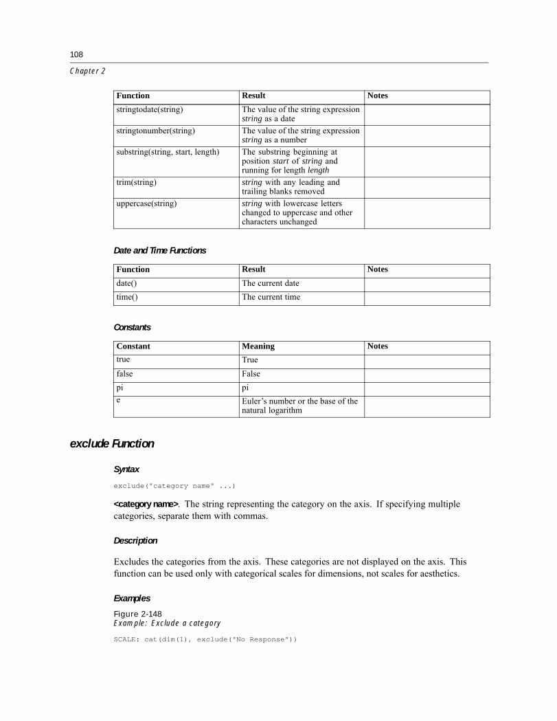
108

Chapter 2

Function Result Notesstringtodate(string) The value of the string expression

string as a datestringtonumber(string) The value of the string expression

string as a numbersubstring(string, start, length) The substring beginning at

position start of string andrunning for length length

trim(string) string with any leading andtrailing blanks removed

uppercase(string) string with lowercase letterschanged to uppercase and othercharacters unchanged

Date and Time Functions

Function Result Notesdate() The current datetime() The current time

Constants

Constant Meaning Notestrue Truefalse Falsepi pie Euler�s number or the base of the

natural logarithm

exclude Function

Syntax

exclude("category name" ...)

<category name>. The string representing the category on the axis. If specifying multiplecategories, separate them with commas.

Description

Excludes the categories from the axis. These categories are not displayed on the axis. Thisfunction can be used only with categorical scales for dimensions, not scales for aesthetics.

Examples

Figure 2-148Example: Exclude a category

SCALE: cat(dim(1), exclude("No Response"))

109


Figure 2-149Example: Excluding multiple categories

SCALE: cat(dim(1), exclude("No Response", "Didn't Ask"))

Applies To

cat Scale

exponent Function

Syntax

exponent(<numeric>)

<numeric>. A numeric value (including negative values) indicating the exponent for the powerscale.

Description

SpeciÞes an exponent for a power scale.

Examples

Figure 2-150Example: Specifying a different power exponent

SCALE: power(dim(2), exponent(3))

exponential Function

Syntax

exponential(<rate>)

<rate>. Numeric value specifying the rate parameter for the distribution.

Description

SpeciÞes an exponential distribution for the probability scale.

Examples

Figure 2-151Example: Specifying an exponential distribution for the probability scale

SCALE: prob(dim(2), exponential(1.5))

Applies To

prob Scale

110

Chapter 2

f Function

Syntax

f(<degrees of freedom>, <degrees of freedom>)

<degrees of freedom>. Numeric values specifying the degrees of freedom parameters for thedistribution. Values must be greater than 0.

Description

SpeciÞes an F distribution for the probability scale.

Examples

SCALE: prob(dim(2), f(5, 2))

Applies To

prob Scale

format Function

Syntax

format("date format")

<format>. The date format of the data.

Description

Indicates the date format for a variable in the source. Use one or more of the followingabbreviations and date separators to indicate the exact format.Table 2-2Abbreviations for date formats

Abbreviation MeaningM Monthd Dayy Yearm Minutes Second

Examples

Figure 2-152Example: Indicating a date format

DATA: date = col(source(mydata), name("date"), unit.time(), format("M/d/yyyy"))

111


Applies To

col Function

from Function

Syntax

from(<variable name>)

<variable name>. The name of a variable previously deÞned in the GPL by a DATA statement.

Description

SpeciÞes one of the pair of nodes that deÞnes an edge relation. The is the node that deÞnes thestarting point for the edge.

Examples

Figure 2-153Example: Creating a directed acyclic graph

ELEMENT: edge(position(layout.dag(node(id), from(fromVar), to(toVar))))

Applies To

layout.circle Function, layout.dag Function, layout.grid Function, layout.network Function,layout.random Function, layout.tree Function

gamma Function

Syntax

gamma(<rate>)

<rate>. Numeric value specifying the shape parameter for the distribution. This values must begreater than 0.

Description

SpeciÞes a gamma distribution for the probability scale.

Examples

Figure 2-154Example: Specifying a gamma distribution for the probability scale

SCALE: prob(dim(2), gamma(2.5))

Applies To

prob Scale

112

Chapter 2

gap Function

Syntax

gap(<value>)

<value>. A number with units (for example, 0px).

Description

SpeciÞes the size of the gap between adjacent axes in a faceted graph. This function is used toclose the space between adjacent axes in population pyramids and matrix scatterplots.

Examples

Figure 2-155Example: Forcing adjacent axes to touch

GUIDE: axis(dim(3), gap(0px))

Applies To

axis Guide Type

gridlines Function

Syntax

gridlines()

Description

SpeciÞes that grid lines should be drawn for the axis. These are lines drawn from the majortick marks to the opposite side of the graph. They can assist in determining the exact locationof a graphic element in the graph.

Examples

Figure 2-156Example: Displaying grid lines

GUIDE: axis(dim(2), gridlines())

Applies To

axis Guide Type

in Function

Syntax

in(min(<value>), max(<value>))

113


<value>. Numeric values for deÞning the range that determines which values to include.

Description

Includes only the continuous values that are in the range speciÞed by the min and max parameters.This function is valid only for continuous variables.

Examples

Figure 2-157Example: Including only a subset of continuous values

DATA: gender = col(source(mydata), name("salary"),in(min(0), max(50000)))

Applies To

col Function

include Function

Syntax

include(<value> ...)

<value>. The string representing the category on the axis or a numeric value on the axis. Ifspecifying multiple values, separate them with commas.

Description

Includes the categories or values on the axis or legend, even if the data do not include thecategories or values. These categories or values are always displayed on the axis or legend. Forexample, you may use include(0) in a bar chart to ensure bars begin at 0.

Examples

Figure 2-158Example: Include a category

SCALE: cat(dim(1), include("No Response"))

Figure 2-159Example: Including multiple categories

SCALE: cat(dim(1), include("No Response", "Didn't Ask"))

Figure 2-160Example: Include a value

SCALE: linear(dim(2), include(0))

Figure 2-161Example: Including multiple values

SCALE: linear(dim(2), include(0, 100))

114

Chapter 2

Applies To

cat Scale, linear Scale, log Scale, pow Scale, safeLog Scale, safePower Scale, time Scale

index Function

Syntax

index()

Description

Creates a new variable by indexing each case with an integer. The new variable is essentiallya case number.

Examples

Figure 2-162Example: Create an index variable and label by the variable

TRANS: casenum = index()ELEMENT: point(position(x*y), label(casenum))

Applies To

TRANS Statement, collapse Function

iter Function

Syntax

iter(<from>, <to>, <step>)

<from>. The Þrst value in the new column. Subsequent values are iterated from this one.

<to>. The maximum value that the new column can contain.

<step>. A value deÞning the amount by which values are iterated.

Description

Creates a new column of data with values in a speciÞed range. Intermediate values are calculatedby adding the step value to the previous value. For example, iter(1,5,1) generates the values1, 2, 3, 4, 5. iter(1,10,2) generates the values 1, 3, 5, 7, 9. Note that 10 is not included in thesecond example because it cannot be iterated from the previous value.

Examples

Figure 2-163Example: Creating a graph from an equation

DATA: x = iter(-100,100,1)TRANS: y = eval(x**2)ELEMENT: line(position(x*y))

115


Applies To

DATA Statement

jump Function

Syntax

jump()

Description

Used with smooth.step, smooth.step.left, smooth.step.center, andsmooth.step.right to indicate that the interpolation line or area jumps to the next value.There is no vertical line connecting the values.

Examples

Figure 2-164Example: Specifying an interpolation line

ELEMENT: line(position(smooth.step(educ*salary)), jump())

Applies To

area Element, line Element

label Function (For Graphic Elements)

Note: If you are modifying the label for a guide (like an axis), refer to label Function (ForGuides) on p. 117.

Syntax

label("label text", <function>)

or

label(<algebra>, <function>)

or

label(<statistic function>, <function>)

“label text”. The text that appears in the label. Multiple strings are concatenated when each stringis separated by a comma (for example, label("This is a ", "long label")).



<statistic function>. A valid statistic function.

116

Chapter 2

Description

SpeciÞes a label for a graphic element. The label appears on the graphic element.

Examples

Figure 2-165Example: Labeling by another variable

ELEMENT: point(position(salbegin*salary), label(gender))

Figure 2-166Example: Labeling by the result of a statistic

ELEMENT: point(position(summary.count(jobcat)), label(summary.count()))

Figure 2-167Example: Labeling by the result of a statistic

ELEMENT: interval(position(summary.mean(jobcat*salary)), label(summary.mean(salary)))

Valid Functions

showAll Function

Statistic Functions


Applies To


117



Note: If you are modifying the label for a graphic element (like a bar or point), refer to labelFunction (For Graphic Elements) on p. 115.

Syntax

label("label text" ...)

“label text”. The text that appears in the label. You can specify multiple strings by separating thestrings with commas (for example, label("This is a ", "long label")). The stringsare concatenated in the resulting graph.

Description

SpeciÞes a label for a guide (for example, an axis or legend). This is text that is displayed onthe resulting graph.

Examples

Figure 2-168Example: Specifying an axis title

GUIDE: axis(dim(1), label("Job Category"))

Figure 2-169Example: Specifying a legend title


Figure 2-170Example: Specifying a graph title

GUIDE: text.title(label("Sales By Region"))

Applies To


layout.circle Function

Note: This function is available only if your SPSS Inc. product is licensed to use it. For SPSSBase users, the function is part of an anticipated advanced visualization add-on module.

Syntax

layout.circle(<function>))

or

layout.circle(<algebra>, <function>)

118

Chapter 2

<algebra>. Graph algebra, such as x*y. Refer to Brief Overview of GPL Algebra on p. 4 foran introduction to graph algebra. The algebra for network graphs is 1*1 because the positionof elements is determined by the layout method and is not tied to a coordinate value (such as avalue on a dimension). This algebra is implied and needs to be speciÞed for network graphsonly when faceting is needed.

<functions>. Valid functions. The from and to functions are required. The node function isoptional for edges, allowing you to draw edges without a separate node data source.

Description

Lays out graphic elements in a circle. The function is used for network graphs, which are visualrepresentations of data that consist of nodes and relations between nodes (edges).

Note: Network graphs that display nodes and edges require two data sources, one for the uniquenodes and one for the edges. If the edge data source includes weights and the weight variable isindicated in the SOURCE statement, the weights inßuence the length of edges in the graph, withhigher weights having shorter edges.

Examples

Figure 2-171Example: Creating a circular network diagram

ELEMENT: edge(position(layout.circle(node(id), from(fromVar), to(toVar))))ELEMENT: point(position(layout.circle(node(id), from(fromVar), to(toVar))), label(id))

Valid Functions

from Function, node Function, to Function

Applies To


119


layout.dag Function


Syntax

layout.dag(<function>))

orlayout.dag(<algebra>, <function>)



Description

Lays out graphic elements as a directed acyclic graph (DAG). The function is used for networkgraphs, which are visual representations of data that consist of nodes and relations between nodes(edges). Other layout options are available for the graph, but the DAG method is appropriatewhen the data are tree-like (directed) and there is no root node.


Examples


ELEMENT: edge(position(layout.dag(node(id), from(fromVar), to(toVar))))ELEMENT: point(position(layout.dag(node(id), from(fromVar), to(toVar))), label(id))

Valid Functions


Applies To

bin.dot Function, bin.hex Function, bin.quantile.letter Function, bin.rect Function, colorFunction (For Graphic Elements), color.brightness Function, color.hue Function, color.saturationFunction, link.alpha Function, link.complete Function, link.delaunay Function, link.distanceFunction, link.gabriel Function, link.hull Function, link.inßuence Function, link.join Function,link.mst Function, link.neighbor Function, link.relativeNeighborhood Function, link.sequence

120

Chapter 2

Function, link.tsp Function, position Function, region.conÞ.count Function, region.conÞ.meanFunction, region.conÞ.percent.count Function, region.spread.range Function, region.spread.sdFunction, region.spread.se Function, size Function, split Function, summary.countFunction, summary.count.cumulative Function, summary.max Function, summary.meanFunction, summary.min Function, summary.percent Function, summary.percent.count,summary.percent.count.cumulative Function, summary.percent.cumulative Function,summary.percent.sum, summary.percent.sum.cumulative Function, summary.sum Function,summary.sum.cumulative Function, transparency Function

layout.grid Function

Syntax

Note: This function is available only if your SPSS Inc. product is licensed to use it. For SPSSBase users, the function is part of an anticipated advanced visualization add-on module.layout.grid(<function>))

orlayout.grid(<algebra>, <function>)



Description

Lays out graphic elements in a grid. The function is used for network graphs, which are visualrepresentations of data that consist of nodes and relations between nodes (edges).


Examples

Figure 2-173Example: Creating a grid network diagram

ELEMENT: edge(position(layout.grid(node(id), from(fromVar), to(toVar))))ELEMENT: point(position(layout.grid(node(id), from(fromVar), to(toVar))), label(id))

Valid Functions


121


Applies To


layout.network Function


Syntax

layout.network(<function>))

or

layout.network(<algebra>, <function>)



Description

Lays out graphic elements in a network. The function is used for network graphs, which arevisual representations of data that consist of nodes and relations between nodes (edges).


122

Chapter 2

Examples

Figure 2-174Example: Creating a network diagram

ELEMENT: edge(position(layout.network(node(id), from(fromVar), to(toVar))))ELEMENT: point(position(layout.network(node(id), from(fromVar), to(toVar))), label(id))

Valid Functions


Applies To


layout.random Function


Syntax

layout.random(<function>))

or

layout.random(<algebra>, <function>)



123


Description

Lays out graphic elements randomly. The function is used for network graphs, which are visualrepresentations of data that consist of nodes and relations between nodes (edges).


Examples

Figure 2-175Example: Creating a random network diagram

ELEMENT: edge(position(layout.random(node(id), from(fromVar), to(toVar))))ELEMENT: point(position(layout.random(node(id), from(fromVar), to(toVar))), label(id))

Valid Functions


Applies To


layout.tree Function


Syntax

layout.tree(<function>))

or

layout.tree(<algebra>, <function>)

124

Chapter 2


<functions>. Valid functions. The from and to functions are required. The node function isoptional for edges, allowing you to draw edges without a separate node data source. Also, youshould use the root function when you want to ensure the correct node is used as the root node.

Description

Lays out graphic elements as a directed tree. The function is used for network graphs, which arevisual representations of data that consist of nodes and relations between nodes (edges). Otherlayout options are available for the graph, but the tree method is appropriate when the data aretree-like (directed) and there is a root node. If the root node is not speciÞed by the root function,the function picks the most likely node as the root.


Examples

Figure 2-176Example: Creating a tree

ELEMENT: edge(position(layout.tree(node(id), from(fromVar), to(toVar), root("A"))))ELEMENT: point(position(layout.tree(node(id), from(fromVar), to(toVar), root("A"))), label(id))

Valid Functions

from Function, node Function, root Function, to Function

Applies To


125


link.alpha Function

Syntax

link.alpha(<algebra>, radius(<numeric>))

orlink.alpha(<binning function>, radius(<numeric>))

orlink.alpha(<statistic function>, radius(<numeric>))


<numeric>. A numeric value indicating the This is required.


<statistic function>. Another statistic function. The result of the embedded statistic is used tocalculate link.alpha.

Description

Calculates the alpha shape for the values. This function is typically used with the edge graphicelement. The alpha shape is a generalization of the convex hull. If the radius is sufÞciently large,the result is a convex hull. For smaller radius values, the shape shrinks and becomes concave. Italso may not connect or contain some data values.

Examples

Figure 2-177Example: Creating an alpha shape graph

ELEMENT: edge(position(link.alpha(x*y, radius(50))))

Binning Functions


Statistic Functions

density.beta Function, density.chiSquare Function, density.exponential Function, density.fFunction, density.gamma Function, density.kernel Function, density.logistic Function,density.normal Function, density.poisson Function, density.studentizedRange Function, density.tFunction, density.uniform Function, density.weibull Function, layout.circle Function, layout.dagFunction, layout.grid Function, layout.network Function, layout.random Function, layout.treeFunction, link.complete Function, link.delaunay Function, link.distance Function, link.gabrielFunction, link.hull Function, link.inßuence Function, link.join Function, link.mst Function,link.neighbor Function, link.relativeNeighborhood Function, link.sequence Function, link.tspFunction, region.conÞ.count Function, region.conÞ.mean Function, region.conÞ.percent.countFunction, region.conÞ.smooth Function, region.spread.range Function, region.spread.sd Function,

126

Chapter 2

region.spread.se Function, smooth.cubic Function, smooth.linear Function, smooth.loessFunction, smooth.mean Function, smooth.median Function, smooth.spline Function, smooth.stepFunction, smooth.quadratic Function, summary.count Function, summary.count.cumulativeFunction, summary.max Function, summary.mean Function, summary.min Function,summary.percent Function, summary.percent.count, summary.percent.count.cumulative Function,summary.percent.cumulative Function, summary.percent.sum, summary.percent.sum.cumulativeFunction, summary.sum Function, summary.sum.cumulative Function

Applies To

bin.dot Function, bin.hex Function, bin.quantile.letter Function, bin.rect Function, color Function(For Graphic Elements), color.brightness Function, color.hue Function, color.saturation Function,link.complete Function, link.delaunay Function, link.distance Function, link.gabriel Function,link.hull Function, link.inßuence Function, link.join Function, link.mst Function, link.neighborFunction, link.relativeNeighborhood Function, link.sequence Function, link.tsp Function, positionFunction, region.conÞ.count Function, region.conÞ.mean Function, region.conÞ.percent.countFunction, region.spread.range Function, region.spread.sd Function, region.spread.seFunction, size Function, split Function, summary.count Function, summary.count.cumulativeFunction, summary.max Function, summary.mean Function, summary.min Function,summary.percent Function, summary.percent.count, summary.percent.count.cumulative Function,summary.percent.cumulative Function, summary.percent.sum, summary.percent.sum.cumulativeFunction, summary.sum Function, summary.sum.cumulative Function, transparency Function

link.complete Function

Syntax

link.complete(<algebra>)

or

link.complete(<binning function>)

or

link.complete(<statistic function>)



<statistic function>. Another statistic function. The result of the embedded statistic is used tocalculate link.complete.

Description

Calculates the complete graph for the values. This function is typically used with the edge graphicelement. The complete graph connects every data value with every other data value.

127


Examples

Figure 2-178Example: Creating a complete graph

ELEMENT: edge(position(link.complete(x*y)))

Binning Functions


Statistic Functions

density.beta Function, density.chiSquare Function, density.exponential Function, density.fFunction, density.gamma Function, density.kernel Function, density.logistic Function,density.normal Function, density.poisson Function, density.studentizedRange Function, density.tFunction, density.uniform Function, density.weibull Function, layout.circle Function, layout.dagFunction, layout.grid Function, layout.network Function, layout.random Function, layout.treeFunction, link.alpha Function, link.delaunay Function, link.distance Function, link.gabrielFunction, link.hull Function, link.inßuence Function, link.join Function, link.mst Function,link.neighbor Function, link.relativeNeighborhood Function, link.sequence Function, link.tspFunction, region.conÞ.count Function, region.conÞ.mean Function, region.conÞ.percent.countFunction, region.conÞ.smooth Function, region.spread.range Function, region.spread.sd Function,region.spread.se Function, smooth.cubic Function, smooth.linear Function, smooth.loessFunction, smooth.mean Function, smooth.median Function, smooth.spline Function, smooth.stepFunction, smooth.quadratic Function, summary.count Function, summary.count.cumulativeFunction, summary.max Function, summary.mean Function, summary.min Function,summary.percent Function, summary.percent.count, summary.percent.count.cumulative Function,summary.percent.cumulative Function, summary.percent.sum, summary.percent.sum.cumulativeFunction, summary.sum Function, summary.sum.cumulative Function

Applies To

bin.dot Function, bin.hex Function, bin.quantile.letter Function, bin.rect Function, color Function(For Graphic Elements), color.brightness Function, color.hue Function, color.saturation Function,link.alpha Function, link.delaunay Function, link.distance Function, link.gabriel Function,link.hull Function, link.inßuence Function, link.join Function, link.mst Function, link.neighborFunction, link.relativeNeighborhood Function, link.sequence Function, link.tsp Function, positionFunction, region.conÞ.count Function, region.conÞ.mean Function, region.conÞ.percent.countFunction, region.spread.range Function, region.spread.sd Function, region.spread.seFunction, size Function, split Function, summary.count Function, summary.count.cumulativeFunction, summary.max Function, summary.mean Function, summary.min Function,summary.percent Function, summary.percent.count, summary.percent.count.cumulative Function,summary.percent.cumulative Function, summary.percent.sum, summary.percent.sum.cumulativeFunction, summary.sum Function, summary.sum.cumulative Function, transparency Function

128

Chapter 2

link.delaunay Function

Syntax

link.delaunay(<algebra>)

or

link.delaunay(<binning function>)

or

link.delaunay(<statistic function>)



<statistic function>. Another statistic function. The result of the embedded statistic is used tocalculate link.delaunay.

Description

Calculates the Delaunay triangulation for the values. This function is typically used with theedge graphic element. The triangulation connects all values so that the connecting segmentsform triangles.

Examples

Figure 2-179Example: Creating a Delaunay triangulation

ELEMENT: edge(position(link.delaunay(x*y)))

Binning Functions


Statistic Functions

density.beta Function, density.chiSquare Function, density.exponential Function, density.fFunction, density.gamma Function, density.kernel Function, density.logistic Function,density.normal Function, density.poisson Function, density.studentizedRange Function, density.tFunction, density.uniform Function, density.weibull Function, layout.circle Function, layout.dagFunction, layout.grid Function, layout.network Function, layout.random Function, layout.treeFunction, link.alpha Function, link.complete Function, link.distance Function, link.gabrielFunction, link.hull Function, link.inßuence Function, link.join Function, link.mst Function,link.neighbor Function, link.relativeNeighborhood Function, link.sequence Function, link.tspFunction, region.conÞ.count Function, region.conÞ.mean Function, region.conÞ.percent.countFunction, region.conÞ.smooth Function, region.spread.range Function, region.spread.sd Function,region.spread.se Function, smooth.cubic Function, smooth.linear Function, smooth.loessFunction, smooth.mean Function, smooth.median Function, smooth.spline Function, smooth.step

129


Function, smooth.quadratic Function, summary.count Function, summary.count.cumulativeFunction, summary.max Function, summary.mean Function, summary.min Function,summary.percent Function, summary.percent.count, summary.percent.count.cumulative Function,summary.percent.cumulative Function, summary.percent.sum, summary.percent.sum.cumulativeFunction, summary.sum Function, summary.sum.cumulative Function

Applies To

bin.dot Function, bin.hex Function, bin.quantile.letter Function, bin.rect Function, color Function(For Graphic Elements), color.brightness Function, color.hue Function, color.saturation Function,link.alpha Function, link.complete Function, link.distance Function, link.gabriel Function,link.hull Function, link.inßuence Function, link.join Function, link.mst Function, link.neighborFunction, link.relativeNeighborhood Function, link.sequence Function, link.tsp Function, positionFunction, region.conÞ.count Function, region.conÞ.mean Function, region.conÞ.percent.countFunction, region.spread.range Function, region.spread.sd Function, region.spread.seFunction, size Function, split Function, summary.count Function, summary.count.cumulativeFunction, summary.max Function, summary.mean Function, summary.min Function,summary.percent Function, summary.percent.count, summary.percent.count.cumulative Function,summary.percent.cumulative Function, summary.percent.sum, summary.percent.sum.cumulativeFunction, summary.sum Function, summary.sum.cumulative Function, transparency Function

link.distance Function

Syntax

link.distance(<algebra>, radius(<numeric>))

or

link.distance(<binning function>, radius(<numeric>))

or

link.distance(<statistic function>, radius(<numeric>))


<numeric>. A numeric value indicating the distance to determine whether values are connected.


<statistic function>. Another statistic function. The result of the embedded statistic is used tocalculate link.distance.

Description

Calculates the distance graph for the values. This function is typically used with the edge graphicelement. The distance graph connects any two values whose distance is less than or equal tothe speciÞed radius.

130

Chapter 2

Examples

Figure 2-180Example: Creating a distance graph

ELEMENT: edge(position(link.distance(x*y), radius(5000)))

Binning Functions


Statistic Functions

density.beta Function, density.chiSquare Function, density.exponential Function, density.fFunction, density.gamma Function, density.kernel Function, density.logistic Function,density.normal Function, density.poisson Function, density.studentizedRange Function, density.tFunction, density.uniform Function, density.weibull Function, layout.circle Function, layout.dagFunction, layout.grid Function, layout.network Function, layout.random Function, layout.treeFunction, link.alpha Function, link.complete Function, link.delaunay Function, link.gabrielFunction, link.hull Function, link.inßuence Function, link.join Function, link.mst Function,link.neighbor Function, link.relativeNeighborhood Function, link.sequence Function, link.tspFunction, region.conÞ.count Function, region.conÞ.mean Function, region.conÞ.percent.countFunction, region.conÞ.smooth Function, region.spread.range Function, region.spread.sd Function,region.spread.se Function, smooth.cubic Function, smooth.linear Function, smooth.loessFunction, smooth.mean Function, smooth.median Function, smooth.spline Function, smooth.stepFunction, smooth.quadratic Function, summary.count Function, summary.count.cumulativeFunction, summary.max Function, summary.mean Function, summary.min Function,summary.percent Function, summary.percent.count, summary.percent.count.cumulative Function,summary.percent.cumulative Function, summary.percent.sum, summary.percent.sum.cumulativeFunction, summary.sum Function, summary.sum.cumulative Function

Applies To

bin.dot Function, bin.hex Function, bin.quantile.letter Function, bin.rect Function, color Function(For Graphic Elements), color.brightness Function, color.hue Function, color.saturation Function,link.alpha Function, link.complete Function, link.delaunay Function, link.gabriel Function,link.hull Function, link.inßuence Function, link.join Function, link.mst Function, link.neighborFunction, link.relativeNeighborhood Function, link.sequence Function, link.tsp Function, positionFunction, region.conÞ.count Function, region.conÞ.mean Function, region.conÞ.percent.countFunction, region.spread.range Function, region.spread.sd Function, region.spread.seFunction, size Function, split Function, summary.count Function, summary.count.cumulativeFunction, summary.max Function, summary.mean Function, summary.min Function,summary.percent Function, summary.percent.count, summary.percent.count.cumulative Function,summary.percent.cumulative Function, summary.percent.sum, summary.percent.sum.cumulativeFunction, summary.sum Function, summary.sum.cumulative Function, transparency Function

131


link.gabriel Function

Syntax

link.gabriel(<algebra>)

or

link.gabriel(<binning function>)

or

link.gabriel(<statistic function>)



<statistic function>. Another statistic function. The result of the embedded statistic is used tocalculate link.gabriel.

Description

Calculates the Gabriel graph for the values. This function is typically used with the edge graphicelement. A Gabriel graph connects values if they are Gabriel neighbors. Gabriel neighbors aredeÞned by imagining a circle whose diameter is the line connecting two values. The values areGabriel neighbors if the circle doesn�t contain any other values.

Examples

Figure 2-181Example: Creating a Gabriel graph

ELEMENT: edge(position(link.gabriel(x*y)))

Binning Functions


Statistic Functions

density.beta Function, density.chiSquare Function, density.exponential Function, density.fFunction, density.gamma Function, density.kernel Function, density.logistic Function,density.normal Function, density.poisson Function, density.studentizedRange Function, density.tFunction, density.uniform Function, density.weibull Function, layout.circle Function, layout.dagFunction, layout.grid Function, layout.network Function, layout.random Function, layout.treeFunction, link.alpha Function, link.complete Function, link.delaunay Function, link.distanceFunction, link.hull Function, link.inßuence Function, link.join Function, link.mst Function,link.neighbor Function, link.relativeNeighborhood Function, link.sequence Function, link.tspFunction, region.conÞ.count Function, region.conÞ.mean Function, region.conÞ.percent.countFunction, region.conÞ.smooth Function, region.spread.range Function, region.spread.sd Function,region.spread.se Function, smooth.cubic Function, smooth.linear Function, smooth.loess

132

Chapter 2

Function, smooth.mean Function, smooth.median Function, smooth.spline Function, smooth.stepFunction, smooth.quadratic Function, summary.count Function, summary.count.cumulativeFunction, summary.max Function, summary.mean Function, summary.min Function,summary.percent Function, summary.percent.count, summary.percent.count.cumulative Function,summary.percent.cumulative Function, summary.percent.sum, summary.percent.sum.cumulativeFunction, summary.sum Function, summary.sum.cumulative Function

Applies To

bin.dot Function, bin.hex Function, bin.quantile.letter Function, bin.rect Function, color Function(For Graphic Elements), color.brightness Function, color.hue Function, color.saturation Function,link.alpha Function, link.complete Function, link.delaunay Function, link.distance Function,link.hull Function, link.inßuence Function, link.join Function, link.mst Function, link.neighborFunction, link.relativeNeighborhood Function, link.sequence Function, link.tsp Function, positionFunction, region.conÞ.count Function, region.conÞ.mean Function, region.conÞ.percent.countFunction, region.spread.range Function, region.spread.sd Function, region.spread.seFunction, size Function, split Function, summary.count Function, summary.count.cumulativeFunction, summary.max Function, summary.mean Function, summary.min Function,summary.percent Function, summary.percent.count, summary.percent.count.cumulative Function,summary.percent.cumulative Function, summary.percent.sum, summary.percent.sum.cumulativeFunction, summary.sum Function, summary.sum.cumulative Function, transparency Function

link.hull Function

Syntax

link.hull(<algebra>)

or

link.hull(<binning function>)

or

link.hull(<statistic function>)



<statistic function>. Another statistic function. The result of the embedded statistic is used tocalculate link.hull.

Description

Calculates the convex hull around the values. This function is typically used with the edgegraphic element. A convex hull connects the least number of outermost values so that the hullcontains all values. The hull contains all possible connections between any two values. Note thatthe convex hull is the boundary of the Delaunay triangulation.

133


Examples

Figure 2-182Example: Creating a convex hull

ELEMENT: edge(position(link.hull(x*y)))

Binning Functions


Statistic Functions

density.beta Function, density.chiSquare Function, density.exponential Function, density.fFunction, density.gamma Function, density.kernel Function, density.logistic Function,density.normal Function, density.poisson Function, density.studentizedRange Function, density.tFunction, density.uniform Function, density.weibull Function, layout.circle Function, layout.dagFunction, layout.grid Function, layout.network Function, layout.random Function, layout.treeFunction, link.alpha Function, link.complete Function, link.delaunay Function, link.distanceFunction, link.gabriel Function, link.inßuence Function, link.join Function, link.mst Function,link.neighbor Function, link.relativeNeighborhood Function, link.sequence Function, link.tspFunction, region.conÞ.count Function, region.conÞ.mean Function, region.conÞ.percent.countFunction, region.conÞ.smooth Function, region.spread.range Function, region.spread.sd Function,region.spread.se Function, smooth.cubic Function, smooth.linear Function, smooth.loessFunction, smooth.mean Function, smooth.median Function, smooth.spline Function, smooth.stepFunction, smooth.quadratic Function, summary.count Function, summary.count.cumulativeFunction, summary.max Function, summary.mean Function, summary.min Function,summary.percent Function, summary.percent.count, summary.percent.count.cumulative Function,summary.percent.cumulative Function, summary.percent.sum, summary.percent.sum.cumulativeFunction, summary.sum Function, summary.sum.cumulative Function

Applies To

bin.dot Function, bin.hex Function, bin.quantile.letter Function, bin.rect Function, color Function(For Graphic Elements), color.brightness Function, color.hue Function, color.saturation Function,link.alpha Function, link.complete Function, link.delaunay Function, link.distance Function,link.gabriel Function, link.inßuence Function, link.join Function, link.mst Function, link.neighborFunction, link.relativeNeighborhood Function, link.sequence Function, link.tsp Function, positionFunction, region.conÞ.count Function, region.conÞ.mean Function, region.conÞ.percent.countFunction, region.spread.range Function, region.spread.sd Function, region.spread.seFunction, size Function, split Function, summary.count Function, summary.count.cumulativeFunction, summary.max Function, summary.mean Function, summary.min Function,summary.percent Function, summary.percent.count, summary.percent.count.cumulative Function,summary.percent.cumulative Function, summary.percent.sum, summary.percent.sum.cumulativeFunction, summary.sum Function, summary.sum.cumulative Function, transparency Function

134

Chapter 2

link.influence Function

Syntax

link.influence(<algebra>)

or

link.influence(<binning function>)

or

link.influence(<statistic function>)



<statistic function>. Another statistic function. The result of the embedded statistic is used tocalculate link.influence.

Description

Calculates a sphere of inßuence graph for the values. This function is typically used with theedge graphic element. The sphere of inßuence graph connects values if the distance between twovalues is less than or equal to the sum of the nearest neighbor distances for the two values. Thenearest neighbor distance for a value is the distance between it and the value closest to it.

Examples

Figure 2-183Example: Creating a sphere of influence graph

ELEMENT: edge(position(link.influence(x*y)))

Binning Functions


Statistic Functions

density.beta Function, density.chiSquare Function, density.exponential Function, density.fFunction, density.gamma Function, density.kernel Function, density.logistic Function,density.normal Function, density.poisson Function, density.studentizedRange Function, density.tFunction, density.uniform Function, density.weibull Function, layout.circle Function, layout.dagFunction, layout.grid Function, layout.network Function, layout.random Function, layout.treeFunction, link.alpha Function, link.complete Function, link.delaunay Function, link.distanceFunction, link.gabriel Function, link.hull Function, link.join Function, link.mst Function,link.neighbor Function, link.relativeNeighborhood Function, link.sequence Function, link.tspFunction, region.conÞ.count Function, region.conÞ.mean Function, region.conÞ.percent.countFunction, region.conÞ.smooth Function, region.spread.range Function, region.spread.sd Function,region.spread.se Function, smooth.cubic Function, smooth.linear Function, smooth.loess

135


Function, smooth.mean Function, smooth.median Function, smooth.spline Function, smooth.stepFunction, smooth.quadratic Function, summary.count Function, summary.count.cumulativeFunction, summary.max Function, summary.mean Function, summary.min Function,summary.percent Function, summary.percent.count, summary.percent.count.cumulative Function,summary.percent.cumulative Function, summary.percent.sum, summary.percent.sum.cumulativeFunction, summary.sum Function, summary.sum.cumulative Function

Applies To

bin.dot Function, bin.hex Function, bin.quantile.letter Function, bin.rect Function, color Function(For Graphic Elements), color.brightness Function, color.hue Function, color.saturation Function,link.alpha Function, link.complete Function, link.delaunay Function, link.distance Function,link.gabriel Function, link.hull Function, link.join Function, link.mst Function, link.neighborFunction, link.relativeNeighborhood Function, link.sequence Function, link.tsp Function, positionFunction, region.conÞ.count Function, region.conÞ.mean Function, region.conÞ.percent.countFunction, region.spread.range Function, region.spread.sd Function, region.spread.seFunction, size Function, split Function, summary.count Function, summary.count.cumulativeFunction, summary.max Function, summary.mean Function, summary.min Function,summary.percent Function, summary.percent.count, summary.percent.count.cumulative Function,summary.percent.cumulative Function, summary.percent.sum, summary.percent.sum.cumulativeFunction, summary.sum Function, summary.sum.cumulative Function, transparency Function

link.join Function

Syntax

link.join(<algebra>)

or

link.join(<binning function>)

or

link.join(<statistic function>)



<statistic function>. Another statistic function. The result of the embedded statistic is used tocalculate link.join.

Description

Joins sets of points from a blend. link.join may be used for repeated measures or observationsover time, among others. In all cases, there is a blend that deÞnes the relation. This distinguisheslink.join from the other link functions.

136

Chapter 2

Examples

Figure 2-184Example: Creating a bridge plot

ELEMENT: edge(position(link.join(x1*y1 + x2*y2)), label(a))ELEMENT: point(position(x1*y1 + x2*y2), label("Before"+"After"))

This example assumes data that is in a format like the following:

Table 2-3Example data

a x1 y1 x2 y2Bill 45 50 58 67Alice 32 40 33 40Bob 22 31 26 35Audrey 55 59 52 64

Figure 2-185Example: Drawing vectors from the origin

TRANS: zero = eval(0)ELEMENT: edge(position(link.join(zero*zero + x*y)), shape(shape.arrow))

Binning Functions


Statistic Functions

density.beta Function, density.chiSquare Function, density.exponential Function, density.fFunction, density.gamma Function, density.kernel Function, density.logistic Function,density.normal Function, density.poisson Function, density.studentizedRange Function, density.tFunction, density.uniform Function, density.weibull Function, layout.circle Function, layout.dagFunction, layout.grid Function, layout.network Function, layout.random Function, layout.treeFunction, link.alpha Function, link.complete Function, link.delaunay Function, link.distanceFunction, link.gabriel Function, link.hull Function, link.inßuence Function, link.mst Function,link.neighbor Function, link.relativeNeighborhood Function, link.sequence Function, link.tspFunction, region.conÞ.count Function, region.conÞ.mean Function, region.conÞ.percent.countFunction, region.conÞ.smooth Function, region.spread.range Function, region.spread.sd Function,region.spread.se Function, smooth.cubic Function, smooth.linear Function, smooth.loessFunction, smooth.mean Function, smooth.median Function, smooth.spline Function, smooth.stepFunction, smooth.quadratic Function, summary.count Function, summary.count.cumulativeFunction, summary.max Function, summary.mean Function, summary.min Function,summary.percent Function, summary.percent.count, summary.percent.count.cumulative Function,summary.percent.cumulative Function, summary.percent.sum, summary.percent.sum.cumulativeFunction, summary.sum Function, summary.sum.cumulative Function

137


Applies To

bin.dot Function, bin.hex Function, bin.quantile.letter Function, bin.rect Function, color Function(For Graphic Elements), color.brightness Function, color.hue Function, color.saturation Function,link.alpha Function, link.complete Function, link.delaunay Function, link.distance Function,link.gabriel Function, link.hull Function, link.inßuence Function, link.mst Function, link.neighborFunction, link.relativeNeighborhood Function, link.sequence Function, link.tsp Function, positionFunction, region.conÞ.count Function, region.conÞ.mean Function, region.conÞ.percent.countFunction, region.spread.range Function, region.spread.sd Function, region.spread.seFunction, size Function, split Function, summary.count Function, summary.count.cumulativeFunction, summary.max Function, summary.mean Function, summary.min Function,summary.percent Function, summary.percent.count, summary.percent.count.cumulative Function,summary.percent.cumulative Function, summary.percent.sum, summary.percent.sum.cumulativeFunction, summary.sum Function, summary.sum.cumulative Function, transparency Function

link.mst Function

Syntax

link.mst(<algebra>)

orlink.mst(<binning function>)

orlink.mst(<statistic function>)



<statistic function>. Another statistic function. The result of the embedded statistic is used tocalculate link.mst.

Description

Calculates the minimum spanning tree (MST) to connect the values speciÞed by the algebra. Thisfunction is typically used with the edge graphic element. The MST connects all values by theshortest distance and never intersects a value twice.

Examples

Figure 2-186Example: Creating a minimal spanning tree

ELEMENT: edge(position(link.mst(x*y)))

Binning Functions


138

Chapter 2

Statistic Functions

density.beta Function, density.chiSquare Function, density.exponential Function, density.fFunction, density.gamma Function, density.kernel Function, density.logistic Function,density.normal Function, density.poisson Function, density.studentizedRange Function, density.tFunction, density.uniform Function, density.weibull Function, layout.circle Function, layout.dagFunction, layout.grid Function, layout.network Function, layout.random Function, layout.treeFunction, link.alpha Function, link.complete Function, link.delaunay Function, link.distanceFunction, link.gabriel Function, link.hull Function, link.inßuence Function, link.join Function,link.neighbor Function, link.relativeNeighborhood Function, link.sequence Function, link.tspFunction, region.conÞ.count Function, region.conÞ.mean Function, region.conÞ.percent.countFunction, region.conÞ.smooth Function, region.spread.range Function, region.spread.sd Function,region.spread.se Function, smooth.cubic Function, smooth.linear Function, smooth.loessFunction, smooth.mean Function, smooth.median Function, smooth.spline Function, smooth.stepFunction, smooth.quadratic Function, summary.count Function, summary.count.cumulativeFunction, summary.max Function, summary.mean Function, summary.min Function,summary.percent Function, summary.percent.count, summary.percent.count.cumulative Function,summary.percent.cumulative Function, summary.percent.sum, summary.percent.sum.cumulativeFunction, summary.sum Function, summary.sum.cumulative Function

Applies To

bin.dot Function, bin.hex Function, bin.quantile.letter Function, bin.rect Function, color Function(For Graphic Elements), color.brightness Function, color.hue Function, color.saturation Function,link.alpha Function, link.complete Function, link.delaunay Function, link.distance Function,link.gabriel Function, link.hull Function, link.inßuence Function, link.join Function, link.neighborFunction, link.relativeNeighborhood Function, link.sequence Function, link.tsp Function, positionFunction, region.conÞ.count Function, region.conÞ.mean Function, region.conÞ.percent.countFunction, region.spread.range Function, region.spread.sd Function, region.spread.seFunction, size Function, split Function, summary.count Function, summary.count.cumulativeFunction, summary.max Function, summary.mean Function, summary.min Function,summary.percent Function, summary.percent.count, summary.percent.count.cumulative Function,summary.percent.cumulative Function, summary.percent.sum, summary.percent.sum.cumulativeFunction, summary.sum Function, summary.sum.cumulative Function, transparency Function

link.neighbor Function

Syntax

link.neighbor(<algebra>, neighborCount(<integer>))

or

link.neighbor(<binning function>, neighborCount(<integer>))

or

link.neighbor(<statistic function>, neighborCount(<integer>))

139



<integer>. An integer deÞning the number of neighboring values to connect to a value.


<statistic function>. Another statistic function. The result of the embedded statistic is used tocalculate link.neighbor.

Description

Calculates the nearest neighbor graph for the values. This function is typically used with the edgegraphic element. The nearest neighbor graph connects a value p to the speciÞed number ofvalues with the shortest distance to p.

Examples

Figure 2-187Example: Creating a nearest neighbor graph

ELEMENT: edge(position(link.neighbor(x*y, neighborCount(3))))

Binning Functions


Statistic Functions

density.beta Function, density.chiSquare Function, density.exponential Function, density.fFunction, density.gamma Function, density.kernel Function, density.logistic Function,density.normal Function, density.poisson Function, density.studentizedRange Function, density.tFunction, density.uniform Function, density.weibull Function, layout.circle Function, layout.dagFunction, layout.grid Function, layout.network Function, layout.random Function, layout.treeFunction, link.alpha Function, link.complete Function, link.delaunay Function, link.distanceFunction, link.gabriel Function, link.hull Function, link.inßuence Function, link.join Function,link.mst Function, link.relativeNeighborhood Function, link.sequence Function, link.tspFunction, region.conÞ.count Function, region.conÞ.mean Function, region.conÞ.percent.countFunction, region.conÞ.smooth Function, region.spread.range Function, region.spread.sd Function,region.spread.se Function, smooth.cubic Function, smooth.linear Function, smooth.loessFunction, smooth.mean Function, smooth.median Function, smooth.spline Function, smooth.stepFunction, smooth.quadratic Function, summary.count Function, summary.count.cumulativeFunction, summary.max Function, summary.mean Function, summary.min Function,summary.percent Function, summary.percent.count, summary.percent.count.cumulative Function,summary.percent.cumulative Function, summary.percent.sum, summary.percent.sum.cumulativeFunction, summary.sum Function, summary.sum.cumulative Function

140

Chapter 2

Applies To

bin.dot Function, bin.hex Function, bin.quantile.letter Function, bin.rect Function, color Function(For Graphic Elements), color.brightness Function, color.hue Function, color.saturation Function,link.alpha Function, link.complete Function, link.delaunay Function, link.distance Function,link.gabriel Function, link.hull Function, link.inßuence Function, link.join Function, link.mstFunction, link.relativeNeighborhood Function, link.sequence Function, link.tsp Function, positionFunction, region.conÞ.count Function, region.conÞ.mean Function, region.conÞ.percent.countFunction, region.spread.range Function, region.spread.sd Function, region.spread.seFunction, size Function, split Function, summary.count Function, summary.count.cumulativeFunction, summary.max Function, summary.mean Function, summary.min Function,summary.percent Function, summary.percent.count, summary.percent.count.cumulative Function,summary.percent.cumulative Function, summary.percent.sum, summary.percent.sum.cumulativeFunction, summary.sum Function, summary.sum.cumulative Function, transparency Function

link.relativeNeighborhood Function

Syntax

link.relativeNeighborhood(<algebra>)

or

link.relativeNeighborhood(<binning function>)

or

link.relativeNeighborhood(<statistic function>)



<statistic function>. Another statistic function. The result of the embedded statistic is used tocalculate link.relativeNeighborhood.

Description

Calculates the relative neighborhood graph for the values. This function is typically used withthe edge graphic element. A relative neighborhood graph connects values if they are relativeneighbors. Relative neighbors are deÞned by imagining two circles whose centers are the twovalues, where the radius of the circles is the distance between the values. If the area created by theintersection of the two circles does not contain any other values, the values are relative neighbors.

Examples

Figure 2-188Example: Creating a relative neighborhood graph

ELEMENT: edge(position(link.relativeNeighborhood(x*y)))

141


Binning Functions


Statistic Functions

density.beta Function, density.chiSquare Function, density.exponential Function, density.fFunction, density.gamma Function, density.kernel Function, density.logistic Function,density.normal Function, density.poisson Function, density.studentizedRange Function,density.t Function, density.uniform Function, density.weibull Function, layout.circle Function,layout.dag Function, layout.grid Function, layout.network Function, layout.random Function,layout.tree Function, link.alpha Function, link.complete Function, link.delaunay Function,link.distance Function, link.gabriel Function, link.hull Function, link.inßuence Function,link.join Function, link.mst Function, link.neighbor Function, link.sequence Function, link.tspFunction, region.conÞ.count Function, region.conÞ.mean Function, region.conÞ.percent.countFunction, region.conÞ.smooth Function, region.spread.range Function, region.spread.sd Function,region.spread.se Function, smooth.cubic Function, smooth.linear Function, smooth.loessFunction, smooth.mean Function, smooth.median Function, smooth.spline Function, smooth.stepFunction, smooth.quadratic Function, summary.count Function, summary.count.cumulativeFunction, summary.max Function, summary.mean Function, summary.min Function,summary.percent Function, summary.percent.count, summary.percent.count.cumulative Function,summary.percent.cumulative Function, summary.percent.sum, summary.percent.sum.cumulativeFunction, summary.sum Function, summary.sum.cumulative Function

Applies To

bin.dot Function, bin.hex Function, bin.quantile.letter Function, bin.rect Function, colorFunction (For Graphic Elements), color.brightness Function, color.hue Function, color.saturationFunction, link.alpha Function, link.complete Function, link.delaunay Function, link.distanceFunction, link.gabriel Function, link.hull Function, link.inßuence Function, link.join Function,link.mst Function, link.neighbor Function, link.sequence Function, link.tsp Function, positionFunction, region.conÞ.count Function, region.conÞ.mean Function, region.conÞ.percent.countFunction, region.spread.range Function, region.spread.sd Function, region.spread.seFunction, size Function, split Function, summary.count Function, summary.count.cumulativeFunction, summary.max Function, summary.mean Function, summary.min Function,summary.percent Function, summary.percent.count, summary.percent.count.cumulative Function,summary.percent.cumulative Function, summary.percent.sum, summary.percent.sum.cumulativeFunction, summary.sum Function, summary.sum.cumulative Function, transparency Function

link.sequence Function

Syntax

link.sequence(<algebra>)

or

link.sequence(<binning function>)

142

Chapter 2

or

link.sequence(<statistic function>)



<statistic function>. Another statistic function. The result of the embedded statistic is used tocalculate link.sequence.

Description

Connects the values in the order in which their associated cases appear in the dataset. Thisfunction is typically used with the edge graphic element. In many cases, the result is the same aswhat you obtain by using the path graphic element without a statistic.

Examples

Figure 2-189Example: Creating a sequence graph

ELEMENT: edge(position(link.sequence(x*y)))

Binning Functions


Statistic Functions

density.beta Function, density.chiSquare Function, density.exponential Function, density.fFunction, density.gamma Function, density.kernel Function, density.logistic Function,density.normal Function, density.poisson Function, density.studentizedRange Function, density.tFunction, density.uniform Function, density.weibull Function, layout.circle Function, layout.dagFunction, layout.grid Function, layout.network Function, layout.random Function, layout.treeFunction, link.alpha Function, link.complete Function, link.delaunay Function, link.distanceFunction, link.gabriel Function, link.hull Function, link.inßuence Function, link.join Function,link.mst Function, link.neighbor Function, link.relativeNeighborhood Function, link.tsp Function,region.conÞ.count Function, region.conÞ.mean Function, region.conÞ.percent.count Function,region.conÞ.smooth Function, region.spread.range Function, region.spread.sd Function,region.spread.se Function, smooth.cubic Function, smooth.linear Function, smooth.loessFunction, smooth.mean Function, smooth.median Function, smooth.spline Function, smooth.stepFunction, smooth.quadratic Function, summary.count Function, summary.count.cumulativeFunction, summary.max Function, summary.mean Function, summary.min Function,summary.percent Function, summary.percent.count, summary.percent.count.cumulative Function,summary.percent.cumulative Function, summary.percent.sum, summary.percent.sum.cumulativeFunction, summary.sum Function, summary.sum.cumulative Function

143


Applies To

bin.dot Function, bin.hex Function, bin.quantile.letter Function, bin.rect Function, color Function(For Graphic Elements), color.brightness Function, color.hue Function, color.saturation Function,link.alpha Function, link.complete Function, link.delaunay Function, link.distance Function,link.gabriel Function, link.hull Function, link.inßuence Function, link.join Function, link.mstFunction, link.neighbor Function, link.relativeNeighborhood Function, link.tsp Function, positionFunction, region.conÞ.count Function, region.conÞ.mean Function, region.conÞ.percent.countFunction, region.spread.range Function, region.spread.sd Function, region.spread.seFunction, size Function, split Function, summary.count Function, summary.count.cumulativeFunction, summary.max Function, summary.mean Function, summary.min Function,summary.percent Function, summary.percent.count, summary.percent.count.cumulative Function,summary.percent.cumulative Function, summary.percent.sum, summary.percent.sum.cumulativeFunction, summary.sum Function, summary.sum.cumulative Function, transparency Function

link.tsp Function

Syntax

link.tsp(<algebra>)

orlink.tsp(<binning function>)

orlink.tsp(<statistic function>)



<statistic function>. Another statistic function. The result of the embedded statistic is used tocalculate link.tsp.

Description

Calculates the solution to the travelling salesman problem (TSP) for the values. This function istypically used with the edge or path graphic element. The solution to the TSP is the shortest paththat traverses all values once and starts and ends at the same value.

Examples

Figure 2-190Example: Drawing the solution to the travelling salesman problem

ELEMENT: edge(position(link.tsp(x*y)))

Binning Functions


144

Chapter 2

Statistic Functions

density.beta Function, density.chiSquare Function, density.exponential Function, density.fFunction, density.gamma Function, density.kernel Function, density.logistic Function,density.normal Function, density.poisson Function, density.studentizedRange Function, density.tFunction, density.uniform Function, density.weibull Function, layout.circle Function, layout.dagFunction, layout.grid Function, layout.network Function, layout.random Function, layout.treeFunction, link.alpha Function, link.complete Function, link.delaunay Function, link.distanceFunction, link.gabriel Function, link.hull Function, link.inßuence Function, link.join Function,link.mst Function, link.neighbor Function, link.relativeNeighborhood Function, link.sequenceFunction, region.conÞ.count Function, region.conÞ.mean Function, region.conÞ.percent.countFunction, region.conÞ.smooth Function, region.spread.range Function, region.spread.sd Function,region.spread.se Function, smooth.cubic Function, smooth.linear Function, smooth.loessFunction, smooth.mean Function, smooth.median Function, smooth.spline Function, smooth.stepFunction, smooth.quadratic Function, summary.count Function, summary.count.cumulativeFunction, summary.max Function, summary.mean Function, summary.min Function,summary.percent Function, summary.percent.count, summary.percent.count.cumulative Function,summary.percent.cumulative Function, summary.percent.sum, summary.percent.sum.cumulativeFunction, summary.sum Function, summary.sum.cumulative Function

Applies To

bin.dot Function, bin.hex Function, bin.quantile.letter Function, bin.rect Function, colorFunction (For Graphic Elements), color.brightness Function, color.hue Function, color.saturationFunction, link.alpha Function, link.complete Function, link.delaunay Function, link.distanceFunction, link.gabriel Function, link.hull Function, link.inßuence Function, link.joinFunction, link.mst Function, link.neighbor Function, link.relativeNeighborhood Function,link.sequence Function, position Function, region.conÞ.count Function, region.conÞ.meanFunction, region.conÞ.percent.count Function, region.spread.range Function, region.spread.sdFunction, region.spread.se Function, size Function, split Function, summary.countFunction, summary.count.cumulative Function, summary.max Function, summary.meanFunction, summary.min Function, summary.percent Function, summary.percent.count,summary.percent.count.cumulative Function, summary.percent.cumulative Function,summary.percent.sum, summary.percent.sum.cumulative Function, summary.sum Function,summary.sum.cumulative Function, transparency Function

logistic Function

Syntax

logistic(<location>, <scale>)

<location>. Numeric value specifying the location parameter for the distribution.

<scale>. Numeric value specifying the scale parameter for the distribution. This value must begreater than 0.

145


Description

SpeciÞes a logistic distribution for the probability scale.

Examples

Figure 2-191Example: Specifying a logistic distribution for the probability scale

SCALE: prob(dim(2), logistic(5, 2))

Applies To

prob Scale

map Function

Syntax

map((<value>, <aesthetic>) ...)

<value>. A categorical value that is being mapped to a speciÞc aesthetic.

<aesthetic>. A valid aesthetic value or constant (for example, color.red or size."5px") thatwill be used for the categorical value.

Note: A value and aesthetic pair is enclosed in parentheses. If you are specifying multiple pairs,use commas to separate the pairs.

Description

Maps a speciÞc categorical value to a speciÞc aesthetic value. For example, if you were creatinga bar chart showing the median income in each U.S. state, you could use the map function toforce the color of the bar corresponding to Illinois to be blue.

Examples

Figure 2-192Example: Mapping a category to a color

SCALE: cat(aesthetic(aesthetic.color), map(("IL", color.blue)))

Figure 2-193Example: Mapping multiple categories to colors

SCALE: cat(aesthetic(aesthetic.color), map(("IL", color.blue), ("CA", color.green)))

Applies To

cat Scale

146

Chapter 2

mapSource Function

Syntax

mapSource(file("file path"), layer("layer name"), key("key name"))

“file path”. The path to the map Þle. This can be an absolute or relative path. The path is relativeto the location of the application that parses the GPL code. Backslashes must be escaped withanother backslash. You can also use forward slashes.

“layer name”. The name of the map layer.

“key name”. The name of a variable in the Þle that acts as a key. This is optional, but you can�tlink the map with a dataset unless you use it.

Description

Reads the contents of an ESRI format map Þle. This function is used to assign the contentsof a speciÞc layer in the Þle to a data source.

Examples

Figure 2-194Example: Reading a map file

SOURCE: mapdata = mapSource(file("C:\\Data\\usStates.smz"), layer("States"), key("STATE"))

Applies To

SOURCE Statement, csvSource Function

mapVariables Function


Syntax

mapVariables(source(<source name>))

<source name>. A map data source previously deÞned by a SOURCE statement and themapSource function.

Description

Extracts the longitude and latitude information from a map data source. Although you can useany name for the result, lon*lat is recommended.

147


Examples

Figure 2-195Example: Using map variables to draw a map

SOURCE: mapdata = mapSource(file("C:\\Data\\usStates.smz"), layer("States"), key("STATE"))DATA: lon*lat = mapVariables(source(mapdata))ELEMENT: polygon(position(lon*lat))

Applies To

DATA Statement

marron Function

Syntax

marron()

Description

Uses the Marron adjustment to normalize the default Þxed window across different kernelfunctions. Different kernel functions have different optimal windows. Therefore, normalizing theÞxed window is useful when you need to compare the results of multiple kernel functions.

Examples

Figure 2-196Example: Adding a kernel distribution

ELEMENT: line(position(density.kernel.epanechnikov(x, marron())))

Applies To


max Function

Syntax

max(<numeric>)

<numeric>. A numeric value indicating the maximum scale value.

Description

SpeciÞes a maximum value for a scale.

Examples

Figure 2-197Example: Specifying a maximum on the 2nd dimension (y axis)


148

Chapter 2

Applies To


min Function

Syntax

min(<numeric>)

<numeric>. A numeric value indicating the minimum scale value.

Description

SpeciÞes a minimum value for a scale.

Examples

Figure 2-198Example: Specifying a minimum on the 2nd dimension (y axis)

SCALE: linear(dim(2), min(0))

Applies To


mirror Function

Syntax

mirror(<coord>)


Description

Mirrors facets in the x axis dimension. This is useful for creating population pyramids.

Examples

Figure 2-199Example: Mirroring dimensions in a population pyramid

COORD: transpose(mirror(rect(dim(1, 2))))


parallel Coordinate Type, polar Coordinate Type, polar.theta Coordinate Type, rect CoordinateType, project Function, reßect Function, transpose Function, wrap Function

149


Applies To

COORD Statement, parallel Coordinate Type, polar Coordinate Type, polar.theta CoordinateType, rect Coordinate Type, project Function

missing.gap Function

Syntax

missing.gap()

Description

SpeciÞes that the graphic element ends at a valid value and does not continue until the next validvalue. There is a gap between valid values.

Examples

Figure 2-200Example: Specifying gaps for missing values

ELEMENT: line(position(x*y), missing.gap())

Applies To


missing.interpolate Function

Syntax

missing.interpolate()

Description

SpeciÞes that the graphic element is interpolated through missing values. That is, the graphicelement is continuous from one valid value to another, regardless of missing values betweenthe valid values.

Examples

Figure 2-201Example: Interpolating through missing values

ELEMENT: line(position(x*y), missing.interpolate())

Applies To


150

Chapter 2

missing.wings Function

Syntax

missing.wings()

Description

SpeciÞes that the graphic element continues after a valid value in the direction of the next validvalue but then breaks just before and after the missing value. This is like interpolating throughthe missing value and erasing the graphic element at the missing value. For line charts, theresult looks similar to wings.

Examples

Figure 2-202Example: Specifying wings for missing values

ELEMENT: line(position(x*y), missing.wings())

Applies To


noConstant Function

Syntax

noConstant()

Description

SpeciÞes that no constant value is used in the smoother equation. Therefore, the smoother iscalculated through the origin.

Examples

Figure 2-203Example: Creating a linear fit line through the origin

ELEMENT: line(position(smooth.linear(salbegin*salary, noConstant())))

Applies To

smooth.linear Function

node Function

Syntax

node(<variable name>)

151



Description

SpeciÞes the variable containing the unique nodes in the dataset.

Examples



Applies To


notIn Function

Syntax

notIn("category name" ...)

<category name>. The string representing the category to be excluded. If specifying multiplecategories, separate them with commas.

Description

Excludes the categories from the variable. These categories are not displayed or used in statisticalcalculations. This function is valid only for variables deÞned as categorical.

Examples

Figure 2-205Example: Excluding a category from a variable

DATA: gender = col(source(mydata), name("gender"), unit.category(), notIn("Missing"))

Applies To

col Function

normal Function

Syntax

normal(<mean>, <standard deviation>)

<mean>. Numeric value indicating the mean parameter for the distribution.

152

Chapter 2

<standard deviation>. Numeric value indicating the standard deviation parameter for thedistribution.

Description

SpeciÞes a normal distribution for the probability scale.

Examples

Figure 2-206Example: Specifying a normal distribution for the probability scale

SCALE: prob(dim(2), normal(50000, 15000))

Applies To

prob Scale

opposite Function

Syntax

opposite()

Description

Positions an axis on the side opposite from the one on which it normally appears. For example,using opposite with the y axis would position it on the right side. opposite can also be usedto create two axes, in which case the opposite one is often an alternate scale or a transformedversion of the original.

Examples

Figure 2-207Example: Moving the y-axis to the opposite side

GUIDE: axis(dim(2), label("Count"), opposite())

Figure 2-208Example: Adding a derived axis

GUIDE: axis(dim(2), label("Cumulative Count"))GUIDE: axis(dim(2), label("Cumulative Percent"), opposite(), unit.percent())

Applies To

axis Guide Type

origin Function (For Graphs)

Note: If you are modifying the origin for a scale, refer to origin Function (For Scales) on p. 153.

153


Syntax

origin(<value>, <value>)

<value>. Indicates an absolute value or a percentage for the origin of the graph. The value isrelative to the top left corner of the page and does not include axis labels. The Þrst value indicatesthe x value relative to this position, and the second value indicates the y value relative to thisposition. Units or a percent sign can be included with the value (e.g., 30px, 5cm, or 25%). If unitsare omitted, they are assumed to be pixels. Percentages are proportional to the whole page.

Description

SpeciÞes the position of the graph relative to the top left corner of the page.

Examples

Figure 2-209Example: Positioning a graph with absolute units

GRAPH: start(origin(2in, 4in))

Figure 2-210Example: Positioning a graph with percentages

GRAPH: start(origin(10%, 100%))

Applies To


origin Function (For Scales)

Note: If you are modifying the origin for a graph, refer to origin Function (For Graphs) on p. 152.

Syntax

origin(<numeric>)

<numeric>. A numeric value indicating the value of the scale�s origin.

Description

SpeciÞes the origin for a scale. The origin is typically used to specify a value from which area orinterval graphic elements extend. The graphic elements originate at the origin and extend towardtheir value. For example, if your bar chart includes values of 367 and 48 and the origin is 100, onebar extends up from 100 to 367 (in default coordinates), while the other bar extends down to 48.

Examples

Figure 2-211Example: Specifying the origin

SCALE: linear(dim(2), origin(100))

154

Chapter 2

Applies To


poisson Function

Syntax

poisson(<rate>)

<rate>. Numeric value specifying the rate parameter for the distribution. This value must begreater than 0.

Description

SpeciÞes a poisson distribution for the probability scale.

Examples

Figure 2-212Example: Specifying a poisson distribution for the probability scale

SCALE: prob(dim(2), poisson(5.5))

Applies To

prob Scale

position Function

Syntax

position(<algebra>)

or

position(<binning function>)

or

position(<statistic function>)




155


Description

SpeciÞes the position of the graphic element in the graph. When a statistic function is used inposition, the statistic function is calculated on the second crossed variable in a 2-D coordinatesystem and the third crossed variable in a 3-D coordinate system.

Examples


ELEMENT: point(position(x*y))

Figure 2-214Example: Bar chart of means

ELEMENT: interval(position(summary.mean(x*y)))

Binning Functions


Statistic Functions


Applies To


156

Chapter 2

preserveStraightLines Function

Syntax

preserveStraightLines()

Description

SpeciÞes that the graphic element is not curved in the space between points. Rather, the graphicelement is drawn straight from point to point. This function is relevant only for graphic elementsdrawn in polar coordinates.

Examples

Figure 2-215Example: Drawing straight lines

ELEMENT: line(position(x*y), preserveStraightLines())

Applies To

area Element, edge Element, line Element, path Element, polygon Element

project Function

Syntax

project.<projection>()

<projection>. A valid projection name.

Description

Transforms the coordinate system using a map projection.

Examples

Figure 2-216Example: Creating a map

SOURCE: mapsrc = mapSource(file("World.smz"), layer("World"))DATA: lon*lat = mapVariables(source(mapsrc))COORD: project.mercator()ELEMENT: polygon(position(lon*lat))

Valid Projection Names

lambertmercatortransverseMercatorwinkelTripel

157


Applies To

COORD Statement, parallel Coordinate Type, polar Coordinate Type, polar.theta CoordinateType, rect Coordinate Type

proportion Function

Syntax

proportion(<numeric>)

<numeric>. A numeric value between 0 and 1.

Description

SpeciÞes the proportion of data points to include when calculating the smooth function. ThisspeciÞes the size of the window used for the smoother.

Examples

Figure 2-217Example: Creating a loess fit line with specific smoother window

ELEMENT: line(position(smooth.loess(salbegin*salary, proportion(0.9))))

Applies To

smooth.cubic Function, smooth.linear Function, smooth.loess Function, smooth.mean Function,smooth.median Function, smooth.quadratic Function

reflect Function

Syntax

reflect(dim(<numeric>), <coord>)

<numeric>. A numeric value indicating the dimension across which the graph is reßected. Formore information, see dim Function on p. 102.


Description

Reßects the coordinate system across the speciÞed dimension.

Examples

Figure 2-218Example: Creating an icicle plot

COORD: rect(dim(1,2), reflect(dim(2)))ELEMENT: interval(position(x*y))

158

Chapter 2


parallel Coordinate Type, polar Coordinate Type, polar.theta Coordinate Type, rect CoordinateType, mirror Function, project Function, transpose Function, wrap Function

Applies To


region.confi.count Function

Syntax

region.confi.count(<algebra>, alpha(<numeric>))

or

region.confi.count(<statistic function>, alpha(<numeric>))

<algebra>. Graph algebra, such as x or x*y. In the second case, the conÞdence interval for thecount is calculated for cases with non-missing y-variable values. Refer to Brief Overview of GPLAlgebra on p. 4 for an introduction to graph algebra.

<statistic function>. Another statistic function. The result of the embedded statistic is used tocalculate region.confi.count.

<numeric>. A numeric value between 0 and 1 indicating the alpha for the conÞdence intervalcalculation. This is optional. If omitted, the alpha is 0.95.

Description

Calculates the conÞdence interval around the count. The function creates two values. When usingthe interval, area, or edge graphic elements, this function results in one graphic elementshowing the range of the conÞdence interval. All other graphic elements result in two separateelements, one showing the conÞdence interval below the count and one showing the conÞdenceinterval above the count.

Examples

Figure 2-219Example: Creating error bars

ELEMENT: interval(position(region.confi.count(jobcat)), shape(shape.ibeam))

Statistic Functions

density.beta Function, density.chiSquare Function, density.exponential Function, density.fFunction, density.gamma Function, density.kernel Function, density.logistic Function,density.normal Function, density.poisson Function, density.studentizedRange Function, density.tFunction, density.uniform Function, density.weibull Function, layout.circle Function, layout.dagFunction, layout.grid Function, layout.network Function, layout.random Function, layout.tree

159


Function, link.alpha Function, link.complete Function, link.delaunay Function, link.distanceFunction, link.gabriel Function, link.hull Function, link.inßuence Function, link.join Function,link.mst Function, link.neighbor Function, link.relativeNeighborhood Function, link.sequenceFunction, link.tsp Function, region.conÞ.mean Function, region.conÞ.percent.count Function,region.conÞ.smooth Function, region.spread.range Function, region.spread.sd Function,region.spread.se Function, smooth.cubic Function, smooth.linear Function, smooth.loessFunction, smooth.mean Function, smooth.median Function, smooth.spline Function, smooth.stepFunction, smooth.quadratic Function, summary.count Function, summary.count.cumulativeFunction, summary.max Function, summary.mean Function, summary.min Function,summary.percent Function, summary.percent.count, summary.percent.count.cumulative Function,summary.percent.cumulative Function, summary.percent.sum, summary.percent.sum.cumulativeFunction, summary.sum Function, summary.sum.cumulative Function

Applies To

bin.dot Function, bin.hex Function, bin.quantile.letter Function, bin.rect Function, color Function(For Graphic Elements), color.brightness Function, color.hue Function, color.saturation Function,link.alpha Function, link.complete Function, link.delaunay Function, link.distance Function,link.gabriel Function, link.hull Function, link.inßuence Function, link.join Function, link.mstFunction, link.neighbor Function, link.relativeNeighborhood Function, link.sequence Function,link.tsp Function, position Function, region.conÞ.mean Function, region.conÞ.percent.countFunction, region.spread.range Function, region.spread.sd Function, region.spread.seFunction, size Function, split Function, summary.count Function, summary.count.cumulativeFunction, summary.max Function, summary.mean Function, summary.min Function,summary.percent Function, summary.percent.count, summary.percent.count.cumulative Function,summary.percent.cumulative Function, summary.percent.sum, summary.percent.sum.cumulativeFunction, summary.sum Function, summary.sum.cumulative Function, transparency Function

region.confi.mean Function

Syntax

region.confi.mean(<algebra>, alpha(<numeric>))

or

region.confi.mean(<statistic function>, alpha(<numeric>))



<statistic function>. Another statistic function. The result of the embedded statistic is used tocalculate region.confi.mean.

160

Chapter 2

Description

Calculates the conÞdence interval around the mean. The function creates two values. When usingthe interval, area, or edge graphic elements, this function results in one graphic elementshowing the range of the conÞdence interval. All other graphic elements result in two separateelements, one showing the conÞdence interval below the mean and one showing the conÞdenceinterval above the mean.

Examples


ELEMENT: interval(position(region.confi.mean(jobcat*salary)), shape(shape.ibeam))

Statistic Functions

density.beta Function, density.chiSquare Function, density.exponential Function, density.fFunction, density.gamma Function, density.kernel Function, density.logistic Function,density.normal Function, density.poisson Function, density.studentizedRange Function, density.tFunction, density.uniform Function, density.weibull Function, layout.circle Function, layout.dagFunction, layout.grid Function, layout.network Function, layout.random Function, layout.treeFunction, link.alpha Function, link.complete Function, link.delaunay Function, link.distanceFunction, link.gabriel Function, link.hull Function, link.inßuence Function, link.join Function,link.mst Function, link.neighbor Function, link.relativeNeighborhood Function, link.sequenceFunction, link.tsp Function, region.conÞ.count Function, region.conÞ.percent.count Function,region.conÞ.smooth Function, region.spread.range Function, region.spread.sd Function,region.spread.se Function, smooth.cubic Function, smooth.linear Function, smooth.loessFunction, smooth.mean Function, smooth.median Function, smooth.spline Function, smooth.stepFunction, smooth.quadratic Function, summary.count Function, summary.count.cumulativeFunction, summary.max Function, summary.mean Function, summary.min Function,summary.percent Function, summary.percent.count, summary.percent.count.cumulative Function,summary.percent.cumulative Function, summary.percent.sum, summary.percent.sum.cumulativeFunction, summary.sum Function, summary.sum.cumulative Function

Applies To

bin.dot Function, bin.hex Function, bin.quantile.letter Function, bin.rect Function, color Function(For Graphic Elements), color.brightness Function, color.hue Function, color.saturation Function,link.alpha Function, link.complete Function, link.delaunay Function, link.distance Function,link.gabriel Function, link.hull Function, link.inßuence Function, link.join Function, link.mstFunction, link.neighbor Function, link.relativeNeighborhood Function, link.sequence Function,link.tsp Function, position Function, region.conÞ.count Function, region.conÞ.percent.countFunction, region.spread.range Function, region.spread.sd Function, region.spread.seFunction, size Function, split Function, summary.count Function, summary.count.cumulativeFunction, summary.max Function, summary.mean Function, summary.min Function,summary.percent Function, summary.percent.count, summary.percent.count.cumulative Function,summary.percent.cumulative Function, summary.percent.sum, summary.percent.sum.cumulativeFunction, summary.sum Function, summary.sum.cumulative Function, transparency Function

161


region.confi.percent.count Function

Syntax

region.confi.percent.count(<algebra>, alpha(<numeric>), <base function>)

orregion.confi.percent.count(<statistic function>, alpha(<numeric>), <base function>)

<algebra>. Graph algebra, such as x or x*y. In the second case, the conÞdence interval for thepercentage is calculated for cases with non-missing y-variable values. Refer to Brief Overviewof GPL Algebra on p. 4 for an introduction to graph algebra.


<base function>. A function that speciÞes the percentage base forregion.confi.percent.count. This is optional. The default is base.all().

<statistic function>. Another statistic function. The result of the embedded statistic is used tocalculate region.confi.percent.count.

Description

Calculates the conÞdence interval around the percentage within each group compared to thetotal number of cases.. The function creates two values. When using the interval, area, oredge graphic elements, this function results in one graphic element showing the range of theconÞdence interval. All other graphic elements result in two separate elements, one showing theconÞdence interval below the percentage valu and one showing the conÞdence interval abovethe percentage valu.

Examples


ELEMENT: interval(position(region.confi.percent.count(jobcat)), shape(shape.ibeam))

Base Functions


Statistic Functions

density.beta Function, density.chiSquare Function, density.exponential Function, density.fFunction, density.gamma Function, density.kernel Function, density.logistic Function,density.normal Function, density.poisson Function, density.studentizedRange Function,density.t Function, density.uniform Function, density.weibull Function, layout.circle Function,layout.dag Function, layout.grid Function, layout.network Function, layout.random Function,layout.tree Function, link.alpha Function, link.complete Function, link.delaunay Function,link.distance Function, link.gabriel Function, link.hull Function, link.inßuence Function, link.joinFunction, link.mst Function, link.neighbor Function, link.relativeNeighborhood Function,

162

Chapter 2

link.sequence Function, link.tsp Function, region.conÞ.count Function, region.conÞ.meanFunction, region.conÞ.smooth Function, region.spread.range Function, region.spread.sd Function,region.spread.se Function, smooth.cubic Function, smooth.linear Function, smooth.loessFunction, smooth.mean Function, smooth.median Function, smooth.spline Function, smooth.stepFunction, smooth.quadratic Function, summary.count Function, summary.count.cumulativeFunction, summary.max Function, summary.mean Function, summary.min Function,summary.percent Function, summary.percent.count, summary.percent.count.cumulative Function,summary.percent.cumulative Function, summary.percent.sum, summary.percent.sum.cumulativeFunction, summary.sum Function, summary.sum.cumulative Function

Applies To

bin.dot Function, bin.hex Function, bin.quantile.letter Function, bin.rect Function, colorFunction (For Graphic Elements), color.brightness Function, color.hue Function, color.saturationFunction, link.alpha Function, link.complete Function, link.delaunay Function, link.distanceFunction, link.gabriel Function, link.hull Function, link.inßuence Function, link.join Function,link.mst Function, link.neighbor Function, link.relativeNeighborhood Function, link.sequenceFunction, link.tsp Function, position Function, region.conÞ.count Function, region.conÞ.meanFunction, region.spread.range Function, region.spread.sd Function, region.spread.seFunction, size Function, split Function, summary.count Function, summary.count.cumulativeFunction, summary.max Function, summary.mean Function, summary.min Function,summary.percent Function, summary.percent.count, summary.percent.count.cumulative Function,summary.percent.cumulative Function, summary.percent.sum, summary.percent.sum.cumulativeFunction, summary.sum Function, summary.sum.cumulative Function, transparency Function

region.confi.smooth Function

Syntax

region.confi.smooth.<smooth function>(<algebra>, alpha(<numeric>))


<smooth function>. The smooth function for which to calculate the conÞdence interval. Validvalues are cubic, linear, and quadratic.


Description

Calculates the conÞdence interval around a smoother function. The function creates two values.When using the interval, area, or edge graphic elements, this function results in one graphicelement showing the range of the conÞdence interval. All other graphic elements result in twoseparate elements, one showing the conÞdence interval below the smoother function and oneshowing the conÞdence interval above the smoother function.

163


Examples

Figure 2-222Example: Showing the confidence interval around a fit line

ELEMENT: line(position(region.confi.smooth.linear(salbegin*salary)))

Applies To


region.spread.range Function

Syntax

region.spread.range(<algebra>)

or

region.spread.range(<statistic function>)


<statistic function>. Another statistic function. The result of the embedded statistic is used tocalculate region.spread.range.

Description

region.spread.range calculates the minimum and maximum for a variable or variablesidentiÞed by the algebra. That is, region.spread.range calculates the range of the variables.When using the interval, area, or edge graphic elements, this function results in one graphicelement showing the range. All other graphic elements result in two separate elements, oneshowing the start of the range and one showing the end of the range.

164

Chapter 2

Examples

Figure 2-223Example: Range bar showing minimum and maximum of one variable

ELEMENT: interval(position(region.spread.range(jobcat*salary)))

Figure 2-224Example: Range bar showing minimum of one variable to maximum of another

ELEMENT: interval(position(region.spread.range(jobcat*(salbegin+salary))))

Statistic Functions

density.beta Function, density.chiSquare Function, density.exponential Function, density.fFunction, density.gamma Function, density.kernel Function, density.logistic Function,density.normal Function, density.poisson Function, density.studentizedRange Function, density.tFunction, density.uniform Function, density.weibull Function, layout.circle Function, layout.dagFunction, layout.grid Function, layout.network Function, layout.random Function, layout.treeFunction, link.alpha Function, link.complete Function, link.delaunay Function, link.distanceFunction, link.gabriel Function, link.hull Function, link.inßuence Function, link.join Function,link.mst Function, link.neighbor Function, link.relativeNeighborhood Function, link.sequenceFunction, link.tsp Function, region.conÞ.count Function, region.conÞ.mean Function,region.conÞ.percent.count Function, region.conÞ.smooth Function, region.spread.sd Function,region.spread.se Function, smooth.cubic Function, smooth.linear Function, smooth.loessFunction, smooth.mean Function, smooth.median Function, smooth.spline Function, smooth.stepFunction, smooth.quadratic Function, summary.count Function, summary.count.cumulativeFunction, summary.max Function, summary.mean Function, summary.min Function,summary.percent Function, summary.percent.count, summary.percent.count.cumulative Function,summary.percent.cumulative Function, summary.percent.sum, summary.percent.sum.cumulativeFunction, summary.sum Function, summary.sum.cumulative Function

Applies To

bin.dot Function, bin.hex Function, bin.quantile.letter Function, bin.rect Function, colorFunction (For Graphic Elements), color.brightness Function, color.hue Function, color.saturationFunction, link.alpha Function, link.complete Function, link.delaunay Function, link.distanceFunction, link.gabriel Function, link.hull Function, link.inßuence Function, link.join Function,link.mst Function, link.neighbor Function, link.relativeNeighborhood Function, link.sequenceFunction, link.tsp Function, position Function, region.conÞ.count Function, region.conÞ.meanFunction, region.conÞ.percent.count Function, region.spread.sd Function, region.spread.seFunction, size Function, split Function, summary.count Function, summary.count.cumulativeFunction, summary.max Function, summary.mean Function, summary.min Function,summary.percent Function, summary.percent.count, summary.percent.count.cumulative Function,summary.percent.cumulative Function, summary.percent.sum, summary.percent.sum.cumulativeFunction, summary.sum Function, summary.sum.cumulative Function, transparency Function

165


region.spread.sd Function

Syntax

region.spread.sd(<algebra>)

or

region.spread.sd(<binning function>)

or

region.spread.sd(<statistic function>)



<statistic function>. Another statistic function. The result of the embedded statistic is used tocalculate region.spread.sd.

Description

region.spread.sd calculates the standard deviation for the variables identiÞed by the algebra.The function creates two values. When using the interval, area, or edge graphic elements,this function results in one graphic element showing the range of the standard deviation aroundthe mean. All other graphic elements result in two separate elements, one showing the standarddeviation below the mean and one showing the standard deviation above the mean.

Examples

Figure 2-225Example: Creating an error bar

ELEMENT: interval(position(region.spread.sd(jobcat*salary)))

Binning Functions


Statistic Functions

density.beta Function, density.chiSquare Function, density.exponential Function, density.fFunction, density.gamma Function, density.kernel Function, density.logistic Function,density.normal Function, density.poisson Function, density.studentizedRange Function, density.tFunction, density.uniform Function, density.weibull Function, layout.circle Function, layout.dagFunction, layout.grid Function, layout.network Function, layout.random Function, layout.treeFunction, link.alpha Function, link.complete Function, link.delaunay Function, link.distanceFunction, link.gabriel Function, link.hull Function, link.inßuence Function, link.join Function,link.mst Function, link.neighbor Function, link.relativeNeighborhood Function, link.sequenceFunction, link.tsp Function, region.conÞ.count Function, region.conÞ.mean Function,region.conÞ.percent.count Function, region.conÞ.smooth Function, region.spread.range Function,

166

Chapter 2

region.spread.se Function, smooth.cubic Function, smooth.linear Function, smooth.loessFunction, smooth.mean Function, smooth.median Function, smooth.spline Function, smooth.stepFunction, smooth.quadratic Function, summary.count Function, summary.count.cumulativeFunction, summary.max Function, summary.mean Function, summary.min Function,summary.percent Function, summary.percent.count, summary.percent.count.cumulative Function,summary.percent.cumulative Function, summary.percent.sum, summary.percent.sum.cumulativeFunction, summary.sum Function, summary.sum.cumulative Function

Applies To

bin.dot Function, bin.hex Function, bin.quantile.letter Function, bin.rect Function, colorFunction (For Graphic Elements), color.brightness Function, color.hue Function, color.saturationFunction, link.alpha Function, link.complete Function, link.delaunay Function, link.distanceFunction, link.gabriel Function, link.hull Function, link.inßuence Function, link.join Function,link.mst Function, link.neighbor Function, link.relativeNeighborhood Function, link.sequenceFunction, link.tsp Function, position Function, region.conÞ.count Function, region.conÞ.meanFunction, region.conÞ.percent.count Function, region.spread.range Function, region.spread.seFunction, size Function, split Function, summary.count Function, summary.count.cumulativeFunction, summary.max Function, summary.mean Function, summary.min Function,summary.percent Function, summary.percent.count, summary.percent.count.cumulative Function,summary.percent.cumulative Function, summary.percent.sum, summary.percent.sum.cumulativeFunction, summary.sum Function, summary.sum.cumulative Function, transparency Function

region.spread.se Function

Syntax

region.spread.se(<algebra>)

or

region.spread.se(<binning function>)

or

region.spread.se(<statistic function>)



<statistic function>. Another statistic function. The result of the embedded statistic is used tocalculate region.spread.se.

Description

region.spread.se calculates the standard error for the variable identiÞed by the algebra. Thefunction creates two values. When using the interval, area, or edge graphic elements, thisfunction results in one graphic element showing the range of the standard error around the mean.

167


All other graphic elements result in two separate elements, one showing the standard error belowthe mean and one showing the standard error above the mean.

Examples

Figure 2-226Example: Creating an error bar

ELEMENT: interval(position(region.spread.se(jobcat*salary)))

Binning Functions


Statistic Functions

density.beta Function, density.chiSquare Function, density.exponential Function, density.fFunction, density.gamma Function, density.kernel Function, density.logistic Function,density.normal Function, density.poisson Function, density.studentizedRange Function, density.tFunction, density.uniform Function, density.weibull Function, layout.circle Function, layout.dagFunction, layout.grid Function, layout.network Function, layout.random Function, layout.treeFunction, link.alpha Function, link.complete Function, link.delaunay Function, link.distanceFunction, link.gabriel Function, link.hull Function, link.inßuence Function, link.join Function,link.mst Function, link.neighbor Function, link.relativeNeighborhood Function, link.sequenceFunction, link.tsp Function, region.conÞ.count Function, region.conÞ.mean Function,region.conÞ.percent.count Function, region.conÞ.smooth Function, region.spread.range Function,region.spread.sd Function, smooth.cubic Function, smooth.linear Function, smooth.loessFunction, smooth.mean Function, smooth.median Function, smooth.spline Function, smooth.stepFunction, smooth.quadratic Function, summary.count Function, summary.count.cumulativeFunction, summary.max Function, summary.mean Function, summary.min Function,summary.percent Function, summary.percent.count, summary.percent.count.cumulative Function,summary.percent.cumulative Function, summary.percent.sum, summary.percent.sum.cumulativeFunction, summary.sum Function, summary.sum.cumulative Function

Applies To

bin.dot Function, bin.hex Function, bin.quantile.letter Function, bin.rect Function, colorFunction (For Graphic Elements), color.brightness Function, color.hue Function, color.saturationFunction, link.alpha Function, link.complete Function, link.delaunay Function, link.distanceFunction, link.gabriel Function, link.hull Function, link.inßuence Function, link.join Function,link.mst Function, link.neighbor Function, link.relativeNeighborhood Function, link.sequenceFunction, link.tsp Function, position Function, region.conÞ.count Function, region.conÞ.meanFunction, region.conÞ.percent.count Function, region.spread.range Function, region.spread.sdFunction, size Function, split Function, summary.count Function, summary.count.cumulativeFunction, summary.max Function, summary.mean Function, summary.min Function,summary.percent Function, summary.percent.count, summary.percent.count.cumulative Function,summary.percent.cumulative Function, summary.percent.sum, summary.percent.sum.cumulativeFunction, summary.sum Function, summary.sum.cumulative Function, transparency Function

168

Chapter 2

reverse Function

Syntax

reverse()

Description

When used in conjunction with a scale, this function reverses the scale. For categorical scales,this function can be used in conjunction with an explicit sorting function.When used in conjunction with a polar coordinate system, this function reverses the direction

of the coordinate system. Thus, it would draw pie slices in a counterclockwise direction.

Examples

Figure 2-227Example: Using reverse alpha-numeric sorting

SCALE: cat(dim(1), sort.natural(), reverse())

Figure 2-228Example: Reversing a linear scale

SCALE: linear(dim(2), reverse())

Figure 2-229Example: Reversing the direction of a coordinate system

COORD: polar.theta(reverse())

Applies To

polar Coordinate Type, polar.theta Coordinate Type, cat Scale, linear Scale, log Scale, pow Scale,safeLog Scale, safePower Scale, time Scale

root Function

Syntax

root("variable value")

“variable value”. A variable value.

Description

SpeciÞes which node is the root node. This corresponds to a value for the variable identiÞedby the node function.

Examples

Figure 2-230Example: Specifying a root node

ELEMENT: edge(position(layout.tree(node(id), from(fromVar), to(toVar), root("A"))))

169


Applies To

layout.tree Function

sameRatio Function

Syntax

sameRatio()

Description

SpeciÞes that the same distance on each scale in a rectangular coordinate system represents thesame difference in data values. For example, 2cm on both scales represent a difference of 1000.

Examples

Figure 2-231Example: Creating a scatterplot with equal scales

COORD: rect(dim(1,2), sameRatio())ELEMENT: point(position(salbegin*salary))

Applies To


scale Function (For Axes)

Note: If you are specifying a size for a graph, refer to scale Function (For Graphs) on p. 170. Ifyou are specifying a scale associated with a graphic element (like a bar or line), refer to scaleFunction (For Graphic Elements) on p. 170. If you are specifying a size for a page, refer toscale Function (For Pages) on p. 171.

Syntax

scale(<scale name>)

<scale name>. A scale previously deÞned by a SCALE statement. This is used when there aremultiple scales in a single dimension (as in a �dual axis� graph).

Description

SpeciÞes the scale to which an axis applies.

Examples

Figure 2-232Example: Associating an axis with a named scale

SCALE: y2= linear(dim(2))GUIDE: axis(scale(y2), label("Count"))

170

Chapter 2

Applies To

axis Guide Type

scale Function (For Graphs)

Note: If you are specifying a scale associated with an axis, refer to scale Function (For Axes)on p. 169. If you are specifying a scale associated with a graphic element (like a bar or line),refer to scale Function (For Graphic Elements) on p. 170. If you are specifying a size for a page,refer to scale Function (For Pages) on p. 171.

Syntax

scale(<value>, <value>)

<value>. Indicates an absolute value or a percentage for the graph size. The Þrst value indicatesthe x component of the size (width), and the second value indicates the y component of the size(height). Units or a percent sign can be included with either value (e.g., 30px, 5cm, or 25%). Ifunits are omitted, they are assumed to be pixels. Percentages are proportional to the whole page.

Description

SpeciÞes the size of the data area of a graph, not including axes and legends.

Examples

Figure 2-233Example: Sizing a graph with absolute units

GRAPH: begin(scale(2in, 4in))

Figure 2-234Example: Sizing a graph with percentages

GRAPH: begin(scale(80%, 100%))

Applies To


scale Function (For Graphic Elements)

Note: If you are specifying a scale associated with an axis, refer to scale Function (For Axes) onp. 169. If you are specifying a size for a graph, refer to scale Function (For Graphs) on p. 170. Ifyou are specifying a size for a page, refer to scale Function (For Pages) on p. 171.

Syntax

scale(<scale name> ...)

171


<scale name>. A scale previously deÞned by a SCALE statement. This is used when there aremultiple scales in a single dimension (as in a �dual-axis� graph). You can specify multiple scalesif the scales are associated with different dimensions. Use commas to separate the multiple scales.

Description

SpeciÞes the scale to which a graphic element applies.

Examples

Figure 2-235Example: Associating a graphic element with a named scale

SCALE: y2= linear(dim(2))ELEMENT: line(scale(y2), position(summary.count(x)))

Applies To


scale Function (For Pages)

Note: If you are specifying a scale associated with an axis, refer to scale Function (For Axes)on p. 169. If you are specifying a scale associated with a graphic element (like a bar or line),refer to scale Function (For Graphic Elements) on p. 170. If you are specifying a size for a graph,refer to scale Function (For Graphs) on p. 170.

Syntax

scale(<value>, <value>)

<value>. Indicates an absolute value for the page size. The Þrst value indicates the x componentof the size (width), and the second value indicates the y component of the size (height). Unitscan be included with either value (e.g., 600px, 15cm, or 5in). If units are omitted, they areassumed to be pixels.

Description

SpeciÞes the size of the graph.

Examples

Figure 2-236Example: Sizing a visualization

PAGE: begin(scale(500px, 400px))

Applies To

begin Function (For Pages)

172

Chapter 2

segments Function

Syntax

segments(<integer>)

<integer>. A positive integer.

Description

SpeciÞes the number of segments that are calculated and drawn for the density function.Excluding this function will result in a default number of segments, which should be sufÞcientfor most cases.

Examples

Figure 2-237Example: Adding a kernel distribution

ELEMENT: line(position(density.kernel.epanechnikov(x, segments(150))))

Applies To


shape Function

Syntax

shape(<algebra>)

or

shape(shape.<constant>)

<algebra>. Graph algebra using one categorical variable or a blend of categorical variables.

<constant>. A constant indicating a speciÞc shape, such as shape.square. For moreinformation, see Shape Constants in Appendix A on p. 280.

Description

Controls the shape of a graphic element. What shape controls depends on the graphic elementtype. The shape of a line speciÞes whether the line is solid or dashed. The border around abar has a similar shape. The shape of a point or interval speciÞes whether the point or intervalis shaped like a square or a line. All of these shapes are controlled by the shape function, butyou can append .interior or .exterior to the function to ensure that you are specifying thedesired one. shape.interior speciÞes the overall shape of the graphic element, including thedashing of line elements. shape.exterior speciÞes the shape of the exterior of the graphicelement, which is often the border on graphic elements with Þlls. Using shape without aqualiÞer implies shape.interior.

173


Examples

Figure 2-238Example: Specifying a shape value

ELEMENT: point(position(salbegin*salary), shape.interior(shape.square))

Figure 2-239Example: Using the values of a variable to control shape

ELEMENT: point(position(salbegin*salary), shape.interior(jobcat))

Figure 2-240Example: Using the values of a variable to control line dashing

ELEMENT: line(position(salbegin*salary), shape.interior(jobcat))

Figure 2-241Example: Using the values of a variable to control border dashing

ELEMENT: interval(position(gender*salary*jobcat), shape.exterior(gender))

Applies To

edge Element, interval Element, line Element, path Element, point Element, polygon Element

showAll Function

Syntax

showAll()

Description

Display all labels, even if they overlap. Without this function, some overlapping labels may notbe displayed, depending on the available space.

Examples

Figure 2-242Example: Displaying all labels

ELEMENT: point(position(x*y), label(z, showAll()))

Applies To

label Function (For Graphic Elements)

size Function

Syntax

size(<algebra>)

or

174

Chapter 2

size(size."size value")

or

size(size.<constant>)

or

size(<statistic function>)

<algebra>. Graph algebra using one variable or a blend of variables. This is not available for lineelements.

“size value”. A speciÞc value that indicates a size. This can be a percentage of the available space(for example, 40%) or a number with units (for example, 2in).

<constant>. A size constant. For more information, see Size Constants in Appendix A on p. 280.


Description

SpeciÞes the size of the individual graphic elements.

Examples

Figure 2-243Example: Using a variable to control size


Figure 2-244Example: Specifying a percentage for size

ELEMENT: interval(position(x*y), size(size."60%"))

Figure 2-245Example: Specifying a value for size

ELEMENT: interval(position(x*y), size(size."6px"))

Figure 2-246Example: Specifying a constant for size

ELEMENT: interval(position(x*y), size(size.large))

Statistic Functions

density.beta Function, density.chiSquare Function, density.exponential Function, density.fFunction, density.gamma Function, density.kernel Function, density.logistic Function,density.normal Function, density.poisson Function, density.studentizedRange Function,density.t Function, density.uniform Function, density.weibull Function, layout.circle Function,layout.dag Function, layout.grid Function, layout.network Function, layout.random Function,layout.tree Function, link.alpha Function, link.complete Function, link.delaunay Function,link.distance Function, link.gabriel Function, link.hull Function, link.inßuence Function, link.joinFunction, link.mst Function, link.neighbor Function, link.relativeNeighborhood Function,link.sequence Function, link.tsp Function, region.conÞ.count Function, region.conÞ.mean

175


Function, region.conÞ.percent.count Function, region.conÞ.smooth Function, region.spread.rangeFunction, region.spread.sd Function, region.spread.se Function, smooth.cubic Function,smooth.linear Function, smooth.loess Function, smooth.mean Function, smooth.median Function,smooth.spline Function, smooth.step Function, smooth.quadratic Function, summary.countFunction, summary.count.cumulative Function, summary.max Function, summary.meanFunction, summary.min Function, summary.percent Function, summary.percent.count,summary.percent.count.cumulative Function, summary.percent.cumulative Function,summary.percent.sum, summary.percent.sum.cumulative Function, summary.sum Function,summary.sum.cumulative Function

Applies To

edge Element, interval Element, line Element, path Element, point Element, polygon Element,schema Element

smooth.cubic Function

Syntax

smooth.cubic(<algebra>, <function>)

or

smooth.cubic.<kernel>(<algebra, <function>)


<kernel>. A kernel function for the smoother. This speciÞes how data are weighted by thesmoother, depending on how close the data are to the current point. If no kernel is speciÞed,Epanechnikov is used.

<function>. One or more valid functions. These are optional. If no proportion function isspeciÞed, 1 is used for the proportion.

Description

Uses regression to determine values that best Þt the data to a cubic polynomial.

Examples

Figure 2-247Example: Creating a cubic fit line

ELEMENT: line(position(smooth.cubic(salbegin*salary)))

176

Chapter 2

Kernel Functions








Valid Functions

proportion Function

Applies To


smooth.linear Function

Syntax

smooth.linear(<algebra>, <function>)

or

smooth.linear.<kernel>(<algebra, <function>)


177




Description

Uses regression to determine values that best Þt the data to a linear slope.

Examples

Figure 2-248Example: Creating a linear fit line

ELEMENT: line(position(smooth.linear(salbegin*salary)))

Kernel Functions








Valid Functions

proportion Function, noConstant Function

Applies To

bin.dot Function, bin.hex Function, bin.quantile.letter Function, bin.rect Function, colorFunction (For Graphic Elements), color.brightness Function, color.hue Function, color.saturationFunction, link.alpha Function, link.complete Function, link.delaunay Function, link.distanceFunction, link.gabriel Function, link.hull Function, link.inßuence Function, link.join Function,link.mst Function, link.neighbor Function, link.relativeNeighborhood Function, link.sequenceFunction, link.tsp Function, position Function, region.conÞ.count Function, region.conÞ.meanFunction, region.conÞ.percent.count Function, region.spread.range Function, region.spread.sdFunction, region.spread.se Function, size Function, split Function, summary.countFunction, summary.count.cumulative Function, summary.max Function, summary.meanFunction, summary.min Function, summary.percent Function, summary.percent.count,

178

Chapter 2

summary.percent.count.cumulative Function, summary.percent.cumulative Function,summary.percent.sum, summary.percent.sum.cumulative Function, summary.sum Function,summary.sum.cumulative Function, transparency Function

smooth.loess Function

Syntax

smooth.loess(<algebra>, <function>)

or

smooth.loess.<kernel>(<algebra>, <function>)


<kernel>. A kernel function for the smoother. This speciÞes how data are weighted by thesmoother, depending on how close the data are to the current point. If no kernel is speciÞed,tricube is used.


Description

Uses iterative weighted least squares to determine values that best Þt the data.

Examples

Figure 2-249Example: Creating a loess fit line

ELEMENT: line(position(smooth.loess(salbegin*salary)))

Figure 2-250Example: Creating a loess fit line with specific kernel

ELEMENT: line(position(smooth.loess.uniform(salbegin*salary)))

Kernel Functions






179




Valid Functions

proportion Function

Applies To


smooth.mean Function

Syntax

smooth.mean(<algebra>, <function>)

or

smooth.mean.<kernel>(<algebra, <function>)




Description

Calculates the smoothed mean of y in a 2-D (x*y) frame and z in a 3-D (x*y*z) frame. To force astraight line (a constant value), use the uniform kernel function.

180

Chapter 2

Examples

Figure 2-251Example: Creating a line at the mean of the y axis

ELEMENT: line(position(smooth.mean.uniform(salbegin*salary)))

Kernel Functions








Valid Functions

proportion Function

Applies To


smooth.median Function

Syntax

smooth.median(<algebra>, <function>)

or

181


smooth.median.<kernel>(<algebra, <function>)




Description

Calculates the smoothed median of y in a 2-D (x*y) frame and z in a 3-D (x*y*z) frame. To forcea straight line (a constant value), use the uniform kernel function.

Examples

Figure 2-252Example: Creating a line at the median of the y axis

ELEMENT: line(position(smooth.median.uniform(salbegin*salary)))

Kernel Functions








Valid Functions

proportion Function

Applies To

bin.dot Function, bin.hex Function, bin.quantile.letter Function, bin.rect Function, colorFunction (For Graphic Elements), color.brightness Function, color.hue Function, color.saturationFunction, link.alpha Function, link.complete Function, link.delaunay Function, link.distanceFunction, link.gabriel Function, link.hull Function, link.inßuence Function, link.join Function,link.mst Function, link.neighbor Function, link.relativeNeighborhood Function, link.sequence

182

Chapter 2

Function, link.tsp Function, position Function, region.conÞ.count Function, region.conÞ.meanFunction, region.conÞ.percent.count Function, region.spread.range Function, region.spread.sdFunction, region.spread.se Function, size Function, split Function, summary.countFunction, summary.count.cumulative Function, summary.max Function, summary.meanFunction, summary.min Function, summary.percent Function, summary.percent.count,summary.percent.count.cumulative Function, summary.percent.cumulative Function,summary.percent.sum, summary.percent.sum.cumulative Function, summary.sum Function,summary.sum.cumulative Function, transparency Function

smooth.spline Function

Syntax

smooth.spline(<algebra>)


Description

Calculates the cubic spline for the data. You should use a cubic spline curve only when youbelieve there is no error in your data.

Examples

Figure 2-253Example: Creating a cubic spline curve

ELEMENT: line(position(smooth.spline(salbegin*salary)))

Applies To


183


smooth.step Function

Syntax

smooth.step(<algebra>)

or

smooth.step.<position>(<algebra>)


<position>. The position of the data value in relation to the drawn line. Valid values are right,left, and center, with right being the default.

Description

Uses step interpolation to draw the graphic element through the data values. Use the jumpfunction to specify that no connecting lines are drawn between the lines at each data value.

Examples

Figure 2-254Example: Creating a step interpolation line

ELEMENT: line(position(smooth.step.center(salbegin*salary)))

Applies To


smooth.quadratic Function

Syntax

smooth.quadratic(<algebra>, <function>)

or

184

Chapter 2

smooth.quadratic.<kernel>(<algebra, <function>)




Description

Uses regression to determine values that best Þt the data to a quadratic polynomial.

Examples

Figure 2-255Example: Creating a quadratic fit line

ELEMENT: line(position(smooth.quadratic(salbegin*salary)))

Kernel Functions








Valid Functions

proportion Function

Applies To

bin.dot Function, bin.hex Function, bin.quantile.letter Function, bin.rect Function, colorFunction (For Graphic Elements), color.brightness Function, color.hue Function, color.saturationFunction, link.alpha Function, link.complete Function, link.delaunay Function, link.distanceFunction, link.gabriel Function, link.hull Function, link.inßuence Function, link.join Function,link.mst Function, link.neighbor Function, link.relativeNeighborhood Function, link.sequenceFunction, link.tsp Function, position Function, region.conÞ.count Function, region.conÞ.mean

185


Function, region.conÞ.percent.count Function, region.spread.range Function, region.spread.sdFunction, region.spread.se Function, size Function, split Function, summary.countFunction, summary.count.cumulative Function, summary.max Function, summary.meanFunction, summary.min Function, summary.percent Function, summary.percent.count,summary.percent.count.cumulative Function, summary.percent.cumulative Function,summary.percent.sum, summary.percent.sum.cumulative Function, summary.sum Function,summary.sum.cumulative Function, transparency Function

sort.data Function

Syntax

sort.data()

Description

Sorts the categorical values in the order they appear in the data.

Note: If the data are pre-aggregated (for example, by using a statistic function in the SPSSGGRAPH command), this function will not work as expected because the categorical values maybe sorted during aggregation. Therefore, the GPL no longer knows the order in which thecategorical values appeared in the original data.

Examples

Figure 2-256Example: Sorting the categories

SCALE: cat(dim(1), sort.data())

Applies To

cat Scale

sort.natural Function

Syntax

sort.natural()

Description

Sorts the categorical values in alphanumeric order.

Examples


SCALE: cat(dim(1), values("Male", "Female"), sort.natural())

186

Chapter 2

Applies To

cat Scale

sort.statistic Function

Syntax

sort.statistic(<statistic function>)


Description

Sorts the categorical values based on the result of the statistic function for each category.

Examples


SCALE: cat(dim(1), sort.statistic(summary.mean(salary)))

Statistic Functions


Applies To

cat Scale

187


sort.values Function

Syntax

sort.values("category name" ...)

“category name”. The name of a category in the data. Delineate each name with a comma.

Description

Sorts the categorical values based on the order in which they appear in this function. You do notneed to specify every category. The categories will be ordered as they appear, and any othercategories that are not speciÞed will appear in the order they appear in the data.

Examples

Figure 2-259Example: Sorting the categories explicitly

SCALE: cat(dim(1), sort.values("Male"))

In this example,Male will appear Þrst. It is not necessary to specify that Female will appear next.

Applies To

cat Scale

split Function

Syntax

split(<algebra>)

or

color(<statistic function>)

<algebra>. The name of a categorical variable.


Description

Splits the graphic element into multiple graphic elements or groups of graphic elements for eachcategory in a categorical variable. This result is similar to that obtained by the aesthetic functions,but there is no speciÞc aesthetic associated with each group of graphic elements.

Examples

Figure 2-260Example: Creating groups of lines

ELEMENT: line(position(salbegin*salary), split(gender))

188

Chapter 2

Statistic Functions


Applies To


start Function

Syntax

start(<value>)

<value>. A numeric value indicating the location of the Þrst major tick.

Description

SpeciÞes the value at which the Þrst major tick appears.

Examples

Figure 2-261Example: Specifying the first major tick

GUIDE: axis(dim(1), start(1000))

Applies To

axis Guide Type

189


startAngle Function

Syntax

startAngle(<integer>)

<integer>. An integer indicating the number of degrees relative to 12:00.

Description

Indicates the angle at which the coordinate system begins. Often used to indicate the position ofthe Þrst slice in a pie chart. The speciÞed degrees are relative to the 12:00 position, and rotationis counterclockwise.

Examples

Figure 2-262Example: Specifying the first slice at 9:00

COORD: polar.theta(startAngle(90))

Figure 2-263Example: Specifying the first slice at 3:00 (90 degrees)

COORD: polar.theta(startAngle(-90))

Applies To

polar Coordinate Type, polar.theta Coordinate Type

studentizedRange Function

Syntax

studentizedRange(<degrees of freedom>, <k>)

<degrees of freedom>. Numeric value indicating the degrees of freedom parameter for thedistribution. The value must be greater than 0.

<k>. Numeric value indicating the k (number of groups) parameter for the distribution. Thevalue must be greater than 0.

Description

SpeciÞes a Studentized range distribution for the probability scale.

Examples

Figure 2-264Example: Specifying a Studentized range distribution for the probability scale

SCALE: prob(dim(2), studentizedRange(5, 2.5))

190

Chapter 2

Applies To

prob Scale

summary.count Function

Syntax

summary.count(<algebra>)

or

summary.count(<binning function>)

or

summary.count(<statistic function>)

<algebra>. Graph algebra, such as x or x*y. In the second case, the count is calculated forcases with non-missing y-variable values. Refer to Brief Overview of GPL Algebra on p. 4for an introduction to graph algebra.


<statistic function>. Another statistic function. The result of the embedded statistic is used tocalculate summary.count.

Description

Calculates the number of cases identiÞed by the algebra or function. If using a function, atypical one would be a binning function. summary.count subsequently calculates the numberof cases in each bin.

Examples

Figure 2-265Example: Specifying a bar chart of counts

ELEMENT: interval(position(summary.count(jobcat)))

Figure 2-266Example: Counting non-missing cases for a continuous variable

ELEMENT: interval(position(summary.count(jobcat*salary)))

Figure 2-267Example: Specifying a histogram

ELEMENT: interval(position(summary.count(bin.rect(salary))))

Binning Functions


191


Statistic Functions

density.beta Function, density.chiSquare Function, density.exponential Function, density.fFunction, density.gamma Function, density.kernel Function, density.logistic Function,density.normal Function, density.poisson Function, density.studentizedRange Function, density.tFunction, density.uniform Function, density.weibull Function, layout.circle Function, layout.dagFunction, layout.grid Function, layout.network Function, layout.random Function, layout.treeFunction, link.alpha Function, link.complete Function, link.delaunay Function, link.distanceFunction, link.gabriel Function, link.hull Function, link.inßuence Function, link.join Function,link.mst Function, link.neighbor Function, link.relativeNeighborhood Function, link.sequenceFunction, link.tsp Function, region.conÞ.count Function, region.conÞ.mean Function,region.conÞ.percent.count Function, region.conÞ.smooth Function, region.spread.range Function,region.spread.sd Function, region.spread.se Function, smooth.cubic Function, smooth.linearFunction, smooth.loess Function, smooth.mean Function, smooth.median Function, smooth.splineFunction, smooth.step Function, smooth.quadratic Function, summary.count.cumulativeFunction, summary.max Function, summary.mean Function, summary.min Function,summary.percent Function, summary.percent.count, summary.percent.count.cumulative Function,summary.percent.cumulative Function, summary.percent.sum, summary.percent.sum.cumulativeFunction, summary.sum Function, summary.sum.cumulative Function

Applies To

bin.dot Function, bin.hex Function, bin.quantile.letter Function, bin.rect Function, colorFunction (For Graphic Elements), color.brightness Function, color.hue Function, color.saturationFunction, link.alpha Function, link.complete Function, link.delaunay Function, link.distanceFunction, link.gabriel Function, link.hull Function, link.inßuence Function, link.join Function,link.mst Function, link.neighbor Function, link.relativeNeighborhood Function, link.sequenceFunction, link.tsp Function, position Function, region.conÞ.count Function, region.conÞ.meanFunction, region.conÞ.percent.count Function, region.spread.range Function, region.spread.sdFunction, region.spread.se Function, size Function, split Function, summary.count.cumulativeFunction, summary.max Function, summary.mean Function, summary.min Function,summary.percent Function, summary.percent.count, summary.percent.count.cumulative Function,summary.percent.cumulative Function, summary.percent.sum, summary.percent.sum.cumulativeFunction, summary.sum Function, summary.sum.cumulative Function, transparency Function

summary.count.cumulative Function

Syntax

summary.count.cumulative(<algebra>)

or

summary.count.cumulative(<binning function>)

or

summary.count.cumulative(<statistic function>)

192

Chapter 2

<algebra>. Graph algebra, such as x or x*y. In the second case, the count is calculated forcases with non-missing y-variable values. Refer to Brief Overview of GPL Algebra on p. 4for an introduction to graph algebra.


<statistic function>. Another statistic function. The result of the embedded statistic is used tocalculate summary.count.cumulative.

Description

Calculates the cumulative number of cases identiÞed by the algebra or function. If using afunction, a typical one would be a binning function. summary.count subsequently calculatesthe number of cases in each bin.If the graph is paneled (faceted), the cumulation begins again with each panel.

Note: If there are multiple ELEMENT statements, you cannot use cumulative statistics for somegraphic elements but not for others. This behavior is prohibited because the results of eachstatistic function would be blended on the same scale. The units for cumulative statistics do notmatch the units for non-cumulative statistics, so blending these results is impossible.

Examples

Figure 2-268Example: Specifying a bar chart of cumulative counts

ELEMENT: interval(position(summary.count.cumulative(jobcat)))

Figure 2-269Example: Specifying a cumulative histogram

ELEMENT: interval(position(summary.count.cumulative(bin.rect(salary))))

Binning Functions


Statistic Functions

density.beta Function, density.chiSquare Function, density.exponential Function, density.fFunction, density.gamma Function, density.kernel Function, density.logistic Function,density.normal Function, density.poisson Function, density.studentizedRange Function,density.t Function, density.uniform Function, density.weibull Function, layout.circle Function,layout.dag Function, layout.grid Function, layout.network Function, layout.random Function,layout.tree Function, link.alpha Function, link.complete Function, link.delaunay Function,link.distance Function, link.gabriel Function, link.hull Function, link.inßuence Function, link.joinFunction, link.mst Function, link.neighbor Function, link.relativeNeighborhood Function,link.sequence Function, link.tsp Function, region.conÞ.count Function, region.conÞ.meanFunction, region.conÞ.percent.count Function, region.conÞ.smooth Function, region.spread.rangeFunction, region.spread.sd Function, region.spread.se Function, smooth.cubic Function,smooth.linear Function, smooth.loess Function, smooth.mean Function, smooth.median Function,smooth.spline Function, smooth.step Function, smooth.quadratic Function, summary.count

193


Function, summary.max Function, summary.mean Function, summary.min Function,summary.percent Function, summary.percent.count, summary.percent.count.cumulative Function,summary.percent.cumulative Function, summary.percent.sum, summary.percent.sum.cumulativeFunction, summary.sum Function, summary.sum.cumulative Function

Applies To

bin.dot Function, bin.hex Function, bin.quantile.letter Function, bin.rect Function, colorFunction (For Graphic Elements), color.brightness Function, color.hue Function, color.saturationFunction, link.alpha Function, link.complete Function, link.delaunay Function, link.distanceFunction, link.gabriel Function, link.hull Function, link.inßuence Function, link.join Function,link.mst Function, link.neighbor Function, link.relativeNeighborhood Function, link.sequenceFunction, link.tsp Function, position Function, region.conÞ.count Function, region.conÞ.meanFunction, region.conÞ.percent.count Function, region.spread.range Function, region.spread.sdFunction, region.spread.se Function, size Function, split Function, summary.countFunction, summary.max Function, summary.mean Function, summary.min Function,summary.percent Function, summary.percent.count, summary.percent.count.cumulative Function,summary.percent.cumulative Function, summary.percent.sum, summary.percent.sum.cumulativeFunction, summary.sum Function, summary.sum.cumulative Function, transparency Function

summary.max Function

Syntax

summary.max(<algebra>)

or

summary.max(<binning function>)

or

summary.max(<statistic function>)



<statistic function>. Another statistic function. The result of the embedded statistic is used tocalculate summary.max.

Description

Calculates the maximum value for variables identiÞed by the algebra. The actual variable whosemaximum is being calculated depends on the coordinate system. In a 2-D coordinate system, itis the second crossed variable in the algebra. In a 3-D coordinate system, it is the third crossedvariable.

194

Chapter 2

Examples

Figure 2-270Example: Calculating the maximum

ELEMENT: interval(position(summary.max(jobcat*salary)))

Binning Functions


Statistic Functions

density.beta Function, density.chiSquare Function, density.exponential Function, density.fFunction, density.gamma Function, density.kernel Function, density.logistic Function,density.normal Function, density.poisson Function, density.studentizedRange Function,density.t Function, density.uniform Function, density.weibull Function, layout.circle Function,layout.dag Function, layout.grid Function, layout.network Function, layout.random Function,layout.tree Function, link.alpha Function, link.complete Function, link.delaunay Function,link.distance Function, link.gabriel Function, link.hull Function, link.inßuence Function, link.joinFunction, link.mst Function, link.neighbor Function, link.relativeNeighborhood Function,link.sequence Function, link.tsp Function, region.conÞ.count Function, region.conÞ.meanFunction, region.conÞ.percent.count Function, region.conÞ.smooth Function, region.spread.rangeFunction, region.spread.sd Function, region.spread.se Function, smooth.cubic Function,smooth.linear Function, smooth.loess Function, smooth.mean Function, smooth.median Function,smooth.spline Function, smooth.step Function, smooth.quadratic Function, summary.countFunction, summary.count.cumulative Function, summary.mean Function, summary.min Function,summary.percent Function, summary.percent.count, summary.percent.count.cumulative Function,summary.percent.cumulative Function, summary.percent.sum, summary.percent.sum.cumulativeFunction, summary.sum Function, summary.sum.cumulative Function

Applies To

bin.dot Function, bin.hex Function, bin.quantile.letter Function, bin.rect Function, colorFunction (For Graphic Elements), color.brightness Function, color.hue Function, color.saturationFunction, link.alpha Function, link.complete Function, link.delaunay Function, link.distanceFunction, link.gabriel Function, link.hull Function, link.inßuence Function, link.join Function,link.mst Function, link.neighbor Function, link.relativeNeighborhood Function, link.sequenceFunction, link.tsp Function, position Function, region.conÞ.count Function, region.conÞ.meanFunction, region.conÞ.percent.count Function, region.spread.range Function, region.spread.sdFunction, region.spread.se Function, size Function, split Function, summary.count Function,summary.count.cumulative Function, summary.mean Function, summary.min Function,summary.percent Function, summary.percent.count, summary.percent.count.cumulative Function,summary.percent.cumulative Function, summary.percent.sum, summary.percent.sum.cumulativeFunction, summary.sum Function, summary.sum.cumulative Function, transparency Function

195


summary.mean Function

Syntax

summary.mean(<algebra>)

or

summary.mean(<binning function>)

or

summary.mean(<statistic function>)



<statistic function>. Another statistic function. The result of the embedded statistic is used tocalculate summary.mean.

Description

Calculates the mean for the variables identiÞed by the algebra. The actual variable whose mean isbeing calculated depends on the coordinate system. In a 2-D coordinate system, it is the secondcrossed variable in the algebra. In a 3-D coordinate system, it is the third crossed variable.

Examples

Figure 2-271Example: Calculating the mean

ELEMENT: interval(position(summary.mean(jobcat*salary)))

Binning Functions


Statistic Functions

density.beta Function, density.chiSquare Function, density.exponential Function, density.fFunction, density.gamma Function, density.kernel Function, density.logistic Function,density.normal Function, density.poisson Function, density.studentizedRange Function,density.t Function, density.uniform Function, density.weibull Function, layout.circle Function,layout.dag Function, layout.grid Function, layout.network Function, layout.random Function,layout.tree Function, link.alpha Function, link.complete Function, link.delaunay Function,link.distance Function, link.gabriel Function, link.hull Function, link.inßuence Function, link.joinFunction, link.mst Function, link.neighbor Function, link.relativeNeighborhood Function,link.sequence Function, link.tsp Function, region.conÞ.count Function, region.conÞ.meanFunction, region.conÞ.percent.count Function, region.conÞ.smooth Function, region.spread.rangeFunction, region.spread.sd Function, region.spread.se Function, smooth.cubic Function,smooth.linear Function, smooth.loess Function, smooth.mean Function, smooth.median Function,

196

Chapter 2

smooth.spline Function, smooth.step Function, smooth.quadratic Function, summary.countFunction, summary.count.cumulative Function, summary.max Function, summary.min Function,summary.percent Function, summary.percent.count, summary.percent.count.cumulative Function,summary.percent.cumulative Function, summary.percent.sum, summary.percent.sum.cumulativeFunction, summary.sum Function, summary.sum.cumulative Function

Applies To

bin.dot Function, bin.hex Function, bin.quantile.letter Function, bin.rect Function, colorFunction (For Graphic Elements), color.brightness Function, color.hue Function, color.saturationFunction, link.alpha Function, link.complete Function, link.delaunay Function, link.distanceFunction, link.gabriel Function, link.hull Function, link.inßuence Function, link.join Function,link.mst Function, link.neighbor Function, link.relativeNeighborhood Function, link.sequenceFunction, link.tsp Function, position Function, region.conÞ.count Function, region.conÞ.meanFunction, region.conÞ.percent.count Function, region.spread.range Function, region.spread.sdFunction, region.spread.se Function, size Function, split Function, summary.count Function,summary.count.cumulative Function, summary.max Function, summary.min Function,summary.percent Function, summary.percent.count, summary.percent.count.cumulative Function,summary.percent.cumulative Function, summary.percent.sum, summary.percent.sum.cumulativeFunction, summary.sum Function, summary.sum.cumulative Function, transparency Function

summary.min Function

Syntax

summary.min(<algebra>)

or

summary.min(<binning function>)

or

summary.min(<statistic function>)



<statistic function>. Another statistic function. The result of the embedded statistic is used tocalculate summary.min.

Description

Calculates the minimum value for variables identiÞed by the algebra. The actual variable whoseminimum is being calculated depends on the coordinate system. In a 2-D coordinate system, itis the second crossed variable in the algebra. In a 3-D coordinate system, it is the third crossedvariable.

197


Examples

Figure 2-272Example: Calculating the minimum

ELEMENT: interval(position(summary.min(jobcat*salary)))

Binning Functions


Statistic Functions

density.beta Function, density.chiSquare Function, density.exponential Function, density.fFunction, density.gamma Function, density.kernel Function, density.logistic Function,density.normal Function, density.poisson Function, density.studentizedRange Function,density.t Function, density.uniform Function, density.weibull Function, layout.circle Function,layout.dag Function, layout.grid Function, layout.network Function, layout.random Function,layout.tree Function, link.alpha Function, link.complete Function, link.delaunay Function,link.distance Function, link.gabriel Function, link.hull Function, link.inßuence Function, link.joinFunction, link.mst Function, link.neighbor Function, link.relativeNeighborhood Function,link.sequence Function, link.tsp Function, region.conÞ.count Function, region.conÞ.meanFunction, region.conÞ.percent.count Function, region.conÞ.smooth Function, region.spread.rangeFunction, region.spread.sd Function, region.spread.se Function, smooth.cubic Function,smooth.linear Function, smooth.loess Function, smooth.mean Function, smooth.median Function,smooth.spline Function, smooth.step Function, smooth.quadratic Function, summary.countFunction, summary.count.cumulative Function, summary.max Function, summary.mean Function,summary.percent Function, summary.percent.count, summary.percent.count.cumulative Function,summary.percent.cumulative Function, summary.percent.sum, summary.percent.sum.cumulativeFunction, summary.sum Function, summary.sum.cumulative Function

Applies To

bin.dot Function, bin.hex Function, bin.quantile.letter Function, bin.rect Function, colorFunction (For Graphic Elements), color.brightness Function, color.hue Function, color.saturationFunction, link.alpha Function, link.complete Function, link.delaunay Function, link.distanceFunction, link.gabriel Function, link.hull Function, link.inßuence Function, link.join Function,link.mst Function, link.neighbor Function, link.relativeNeighborhood Function, link.sequenceFunction, link.tsp Function, position Function, region.conÞ.count Function, region.conÞ.meanFunction, region.conÞ.percent.count Function, region.spread.range Function, region.spread.sdFunction, region.spread.se Function, size Function, split Function, summary.count Function,summary.count.cumulative Function, summary.max Function, summary.mean Function,summary.percent Function, summary.percent.count, summary.percent.count.cumulative Function,summary.percent.cumulative Function, summary.percent.sum, summary.percent.sum.cumulativeFunction, summary.sum Function, summary.sum.cumulative Function, transparency Function

198

Chapter 2

summary.percent Function

Description

summary.percent is an alias for summary.percent.sum. For more information, seesummary.percent.sum on p. 202.

Examples

Figure 2-273Example: Calculating percentages of a summed variable

ELEMENT: interval(position(summary.percent(jobcat*salary)))

Applies To

bin.dot Function, bin.hex Function, bin.quantile.letter Function, bin.rect Function, colorFunction (For Graphic Elements), color.brightness Function, color.hue Function, color.saturationFunction, link.alpha Function, link.complete Function, link.delaunay Function, link.distanceFunction, link.gabriel Function, link.hull Function, link.inßuence Function, link.join Function,link.mst Function, link.neighbor Function, link.relativeNeighborhood Function, link.sequenceFunction, link.tsp Function, position Function, region.conÞ.count Function, region.conÞ.meanFunction, region.conÞ.percent.count Function, region.spread.range Function, region.spread.sdFunction, region.spread.se Function, size Function, split Function, summary.count Function,summary.count.cumulative Function, summary.max Function, summary.mean Function,summary.min Function, summary.percent.count, summary.percent.count.cumulative Function,summary.percent.cumulative Function, summary.percent.sum, summary.percent.sum.cumulativeFunction, summary.sum Function, summary.sum.cumulative Function, transparency Function

summary.percent.count

Syntax

summary.percent.count(<algebra>, <base function>)

or

summary.percent.count(<statistic function>, <base function>)

<algebra>. Graph algebra, such as x or x*y. In the second case, the percentage is calculated forcases with non-missing y-variable values. Refer to Brief Overview of GPL Algebra on p. 4for an introduction to graph algebra.

<base function>. A function that speciÞes the percentage base for summary.percent.count.This is optional. The default is base.all().

<statistic function>. Another statistic function. The result of the embedded statistic is used tocalculate summary.percent.count.

199


Description

Calculates the percentage within each group compared to the total number of cases.

Examples

Figure 2-274Example: Calculating percentages of counts

ELEMENT: interval(position(summary.percent.count(jobcat)))

Base Functions


Binning Functions


Statistic Functions

density.beta Function, density.chiSquare Function, density.exponential Function, density.fFunction, density.gamma Function, density.kernel Function, density.logistic Function,density.normal Function, density.poisson Function, density.studentizedRange Function,density.t Function, density.uniform Function, density.weibull Function, layout.circle Function,layout.dag Function, layout.grid Function, layout.network Function, layout.random Function,layout.tree Function, link.alpha Function, link.complete Function, link.delaunay Function,link.distance Function, link.gabriel Function, link.hull Function, link.inßuence Function, link.joinFunction, link.mst Function, link.neighbor Function, link.relativeNeighborhood Function,link.sequence Function, link.tsp Function, region.conÞ.count Function, region.conÞ.meanFunction, region.conÞ.percent.count Function, region.conÞ.smooth Function, region.spread.rangeFunction, region.spread.sd Function, region.spread.se Function, smooth.cubic Function,smooth.linear Function, smooth.loess Function, smooth.mean Function, smooth.median Function,smooth.spline Function, smooth.step Function, smooth.quadratic Function, summary.countFunction, summary.count.cumulative Function, summary.max Function, summary.mean Function,summary.min Function, summary.percent Function, summary.percent.count.cumulative Function,summary.percent.cumulative Function, summary.percent.sum, summary.percent.sum.cumulativeFunction, summary.sum Function, summary.sum.cumulative Function

Applies To

bin.dot Function, bin.hex Function, bin.quantile.letter Function, bin.rect Function, colorFunction (For Graphic Elements), color.brightness Function, color.hue Function, color.saturationFunction, link.alpha Function, link.complete Function, link.delaunay Function, link.distanceFunction, link.gabriel Function, link.hull Function, link.inßuence Function, link.join Function,link.mst Function, link.neighbor Function, link.relativeNeighborhood Function, link.sequenceFunction, link.tsp Function, position Function, region.conÞ.count Function, region.conÞ.meanFunction, region.conÞ.percent.count Function, region.spread.range Function, region.spread.sdFunction, region.spread.se Function, size Function, split Function, summary.count Function,summary.count.cumulative Function, summary.max Function, summary.mean Function,

200

Chapter 2

summary.min Function, summary.percent Function, summary.percent.count.cumulative Function,summary.percent.cumulative Function, summary.percent.sum, summary.percent.sum.cumulativeFunction, summary.sum Function, summary.sum.cumulative Function, transparency Function

summary.percent.count.cumulative Functionsummary.percent.count.cumulative(<algebra>, <base function>)

orsummary.percent.count.cumulative(<statistic function>, <base function>)

<algebra>. Graph algebra, such as x or x*y. In the second case, the percentage is calculated forcases with non-missing y-variable values. Refer to Brief Overview of GPL Algebra on p. 4for an introduction to graph algebra.

<base function>. A function that speciÞes the percentage base forsummary.percent.count.cumulative. This is optional. The default is base.all().

<statistic function>. Another statistic function. The result of the embedded statistic is used tocalculate summary.percent.count.cumulative.

Description

Calculates the cumulative percentage within each group compared to the total number of cases.


Examples

Figure 2-275Example: Calculating cumulative percentages of counts

ELEMENT: interval(position(summary.percent.count.cumulative(jobcat)))

Base Functions


Binning Functions


Statistic Functions

density.beta Function, density.chiSquare Function, density.exponential Function, density.fFunction, density.gamma Function, density.kernel Function, density.logistic Function,density.normal Function, density.poisson Function, density.studentizedRange Function,density.t Function, density.uniform Function, density.weibull Function, layout.circle Function,layout.dag Function, layout.grid Function, layout.network Function, layout.random Function,

201


layout.tree Function, link.alpha Function, link.complete Function, link.delaunay Function,link.distance Function, link.gabriel Function, link.hull Function, link.inßuence Function, link.joinFunction, link.mst Function, link.neighbor Function, link.relativeNeighborhood Function,link.sequence Function, link.tsp Function, region.conÞ.count Function, region.conÞ.meanFunction, region.conÞ.percent.count Function, region.conÞ.smooth Function, region.spread.rangeFunction, region.spread.sd Function, region.spread.se Function, smooth.cubic Function,smooth.linear Function, smooth.loess Function, smooth.mean Function, smooth.median Function,smooth.spline Function, smooth.step Function, smooth.quadratic Function, summary.countFunction, summary.count.cumulative Function, summary.max Function, summary.meanFunction, summary.min Function, summary.percent Function, summary.percent.count,summary.percent.cumulative Function, summary.percent.sum, summary.percent.sum.cumulativeFunction, summary.sum Function, summary.sum.cumulative Function

Applies To

bin.dot Function, bin.hex Function, bin.quantile.letter Function, bin.rect Function, colorFunction (For Graphic Elements), color.brightness Function, color.hue Function, color.saturationFunction, link.alpha Function, link.complete Function, link.delaunay Function, link.distanceFunction, link.gabriel Function, link.hull Function, link.inßuence Function, link.join Function,link.mst Function, link.neighbor Function, link.relativeNeighborhood Function, link.sequenceFunction, link.tsp Function, position Function, region.conÞ.count Function, region.conÞ.meanFunction, region.conÞ.percent.count Function, region.spread.range Function, region.spread.sdFunction, region.spread.se Function, size Function, split Function, summary.countFunction, summary.count.cumulative Function, summary.max Function, summary.meanFunction, summary.min Function, summary.percent Function, summary.percent.count,summary.percent.cumulative Function, summary.percent.sum, summary.percent.sum.cumulativeFunction, summary.sum Function, summary.sum.cumulative Function, transparency Function

summary.percent.cumulative Function

Description

summary.percent.cumulative is an alias for summary.percent.sum.cumulative. Formore information, see summary.percent.sum.cumulative Function on p. 203.


Examples

Figure 2-276Example: Calculating cumulative percentages of a summed variable

ELEMENT: interval(position(summary.percent.cumulative(jobcat*salary)))

202

Chapter 2

summary.percent.sum

Syntax

summary.percent.sum(<algebra>, <base function>)

orsummary.percent.sum(<statistic function>, <base function>)


<base function>. A function that speciÞes the percentage base for summary.percent.sum.This is optional. The default is base.all().

<statistic function>. Another statistic function. The result of the embedded statistic is used tocalculate summary.percent.sum.

Description

Calculates the percentage within each group based on a summed variable compared tothe sum across all groups. summary.percent is an alias for this function. To obtainpercentages of counts, use the summary.percent.count function. For more information, seesummary.percent.count on p. 198.

Examples

Figure 2-277Example: Calculating percentages of a summed variable

ELEMENT: interval(position(summary.percent.sum(jobcat*salary)))

Base Functions


Binning Functions


Statistic Functions

density.beta Function, density.chiSquare Function, density.exponential Function, density.fFunction, density.gamma Function, density.kernel Function, density.logistic Function,density.normal Function, density.poisson Function, density.studentizedRange Function,density.t Function, density.uniform Function, density.weibull Function, layout.circle Function,layout.dag Function, layout.grid Function, layout.network Function, layout.random Function,layout.tree Function, link.alpha Function, link.complete Function, link.delaunay Function,link.distance Function, link.gabriel Function, link.hull Function, link.inßuence Function, link.joinFunction, link.mst Function, link.neighbor Function, link.relativeNeighborhood Function,link.sequence Function, link.tsp Function, region.conÞ.count Function, region.conÞ.meanFunction, region.conÞ.percent.count Function, region.conÞ.smooth Function, region.spread.range

203


Function, region.spread.sd Function, region.spread.se Function, smooth.cubic Function,smooth.linear Function, smooth.loess Function, smooth.mean Function, smooth.median Function,smooth.spline Function, smooth.step Function, smooth.quadratic Function, summary.countFunction, summary.count.cumulative Function, summary.max Function, summary.meanFunction, summary.min Function, summary.percent Function, summary.percent.count,summary.percent.count.cumulative Function, summary.percent.cumulative Function,summary.percent.sum.cumulative Function, summary.sum Function, summary.sum.cumulativeFunction

Applies To

bin.dot Function, bin.hex Function, bin.quantile.letter Function, bin.rect Function, colorFunction (For Graphic Elements), color.brightness Function, color.hue Function, color.saturationFunction, link.alpha Function, link.complete Function, link.delaunay Function, link.distanceFunction, link.gabriel Function, link.hull Function, link.inßuence Function, link.join Function,link.mst Function, link.neighbor Function, link.relativeNeighborhood Function, link.sequenceFunction, link.tsp Function, position Function, region.conÞ.count Function, region.conÞ.meanFunction, region.conÞ.percent.count Function, region.spread.range Function, region.spread.sdFunction, region.spread.se Function, size Function, split Function, summary.countFunction, summary.count.cumulative Function, summary.max Function, summary.meanFunction, summary.min Function, summary.percent Function, summary.percent.count,summary.percent.count.cumulative Function, summary.percent.cumulative Function,summary.percent.sum.cumulative Function, summary.sum Function, summary.sum.cumulativeFunction, transparency Function

summary.percent.sum.cumulative Function

summary.percent.sum.cumulative(<algebra>, <base function>)

or

summary.percent.sum.cumulative(<statistic function>, <base function>)


<base function>. A function that speciÞes the percentage base forsummary.percent.sum.cumulative. This is optional. The default is base.all().

<statistic function>. Another statistic function. The result of the embedded statistic is used tocalculate summary.percent.sum.cumulative.

Description

Calculates the cumulative percentage within each group based on a summed variable compared tothe sum across all groups. summary.percent.cumulative is an alias for this function. Toobtain cumulative percentages of counts, use the summary.percent.count.cumulativefunction. For more information, see summary.percent.count.cumulative Function on p. 200.

204

Chapter 2


Examples

Figure 2-278Example: Calculating cumulative percentages of a summed variable

ELEMENT: interval(position(summary.percent.sum.cumulative(jobcat*salary)))

Base Functions


Binning Functions


Statistic Functions

density.beta Function, density.chiSquare Function, density.exponential Function, density.fFunction, density.gamma Function, density.kernel Function, density.logistic Function,density.normal Function, density.poisson Function, density.studentizedRange Function,density.t Function, density.uniform Function, density.weibull Function, layout.circle Function,layout.dag Function, layout.grid Function, layout.network Function, layout.random Function,layout.tree Function, link.alpha Function, link.complete Function, link.delaunay Function,link.distance Function, link.gabriel Function, link.hull Function, link.inßuence Function, link.joinFunction, link.mst Function, link.neighbor Function, link.relativeNeighborhood Function,link.sequence Function, link.tsp Function, region.conÞ.count Function, region.conÞ.meanFunction, region.conÞ.percent.count Function, region.conÞ.smooth Function, region.spread.rangeFunction, region.spread.sd Function, region.spread.se Function, smooth.cubic Function,smooth.linear Function, smooth.loess Function, smooth.mean Function, smooth.median Function,smooth.spline Function, smooth.step Function, smooth.quadratic Function, summary.countFunction, summary.count.cumulative Function, summary.max Function, summary.meanFunction, summary.min Function, summary.percent Function, summary.percent.count,summary.percent.count.cumulative Function, summary.percent.cumulative Function,summary.percent.sum, summary.sum Function, summary.sum.cumulative Function

Applies To

bin.dot Function, bin.hex Function, bin.quantile.letter Function, bin.rect Function, colorFunction (For Graphic Elements), color.brightness Function, color.hue Function, color.saturationFunction, link.alpha Function, link.complete Function, link.delaunay Function, link.distanceFunction, link.gabriel Function, link.hull Function, link.inßuence Function, link.join Function,link.mst Function, link.neighbor Function, link.relativeNeighborhood Function, link.sequenceFunction, link.tsp Function, position Function, region.conÞ.count Function, region.conÞ.meanFunction, region.conÞ.percent.count Function, region.spread.range Function, region.spread.sdFunction, region.spread.se Function, size Function, split Function, summary.count

205


Function, summary.count.cumulative Function, summary.max Function, summary.meanFunction, summary.min Function, summary.percent Function, summary.percent.count,summary.percent.count.cumulative Function, summary.percent.cumulative Function,summary.percent.sum, summary.sum Function, summary.sum.cumulative Function, transparencyFunction

summary.sum Function

Syntax

summary.sum(<algebra>)

orsummary.sum(<binning function>)

orsummary.sum(<statistic function>)



<statistic function>. Another statistic function. The result of the embedded statistic is used tocalculate summary.sum.

Description

Calculates the sum for the variables identiÞed by the algebra. The actual variable being summeddepends on the coordinate system. In a 2-D coordinate system, it is the second crossed variable inthe algebra. In a 3-D coordinate system, it is the third crossed variable.

Examples

Figure 2-279Example: Calculating the sum

ELEMENT: interval(position(summary.sum(jobcat*salary)))

Binning Functions


Statistic Functions

density.beta Function, density.chiSquare Function, density.exponential Function, density.fFunction, density.gamma Function, density.kernel Function, density.logistic Function,density.normal Function, density.poisson Function, density.studentizedRange Function,density.t Function, density.uniform Function, density.weibull Function, layout.circle Function,layout.dag Function, layout.grid Function, layout.network Function, layout.random Function,layout.tree Function, link.alpha Function, link.complete Function, link.delaunay Function,

206

Chapter 2

link.distance Function, link.gabriel Function, link.hull Function, link.inßuence Function, link.joinFunction, link.mst Function, link.neighbor Function, link.relativeNeighborhood Function,link.sequence Function, link.tsp Function, region.conÞ.count Function, region.conÞ.meanFunction, region.conÞ.percent.count Function, region.conÞ.smooth Function, region.spread.rangeFunction, region.spread.sd Function, region.spread.se Function, smooth.cubic Function,smooth.linear Function, smooth.loess Function, smooth.mean Function, smooth.median Function,smooth.spline Function, smooth.step Function, smooth.quadratic Function, summary.countFunction, summary.count.cumulative Function, summary.max Function, summary.meanFunction, summary.min Function, summary.percent Function, summary.percent.count,summary.percent.count.cumulative Function, summary.percent.cumulative Function,summary.percent.sum, summary.percent.sum.cumulative Function, summary.sum.cumulativeFunction

Applies To

bin.dot Function, bin.hex Function, bin.quantile.letter Function, bin.rect Function, colorFunction (For Graphic Elements), color.brightness Function, color.hue Function, color.saturationFunction, link.alpha Function, link.complete Function, link.delaunay Function, link.distanceFunction, link.gabriel Function, link.hull Function, link.inßuence Function, link.join Function,link.mst Function, link.neighbor Function, link.relativeNeighborhood Function, link.sequenceFunction, link.tsp Function, position Function, region.conÞ.count Function, region.conÞ.meanFunction, region.conÞ.percent.count Function, region.spread.range Function, region.spread.sdFunction, region.spread.se Function, size Function, split Function, summary.countFunction, summary.count.cumulative Function, summary.max Function, summary.meanFunction, summary.min Function, summary.percent Function, summary.percent.count,summary.percent.count.cumulative Function, summary.percent.cumulative Function,summary.percent.sum, summary.percent.sum.cumulative Function, summary.sum.cumulativeFunction, transparency Function

summary.sum.cumulative Function

Syntax

summary.sum.cumulative(<algebra>)

or

summary.sum.cumulative(<binning function>)

or

summary.sum.cumulative(<statistic function>)



<statistic function>. Another statistic function. The result of the embedded statistic is used tocalculate summary.sum.cumulative.

207


Description

Calculates the cumulative sum for the variables identiÞed by the algebra. The actual variablebeing summed depends on the coordinate system. In a 2-D coordinate system, it is the secondcrossed variable in the algebra. In a 3-D coordinate system, it is the third crossed variable.


Examples

Figure 2-280Example: Calculating the cumulative sum

ELEMENT: interval(position(summary.sum(jobcat*salary)))

Binning Functions


Statistic Functions

density.beta Function, density.chiSquare Function, density.exponential Function, density.fFunction, density.gamma Function, density.kernel Function, density.logistic Function,density.normal Function, density.poisson Function, density.studentizedRange Function,density.t Function, density.uniform Function, density.weibull Function, layout.circle Function,layout.dag Function, layout.grid Function, layout.network Function, layout.random Function,layout.tree Function, link.alpha Function, link.complete Function, link.delaunay Function,link.distance Function, link.gabriel Function, link.hull Function, link.inßuence Function, link.joinFunction, link.mst Function, link.neighbor Function, link.relativeNeighborhood Function,link.sequence Function, link.tsp Function, region.conÞ.count Function, region.conÞ.meanFunction, region.conÞ.percent.count Function, region.conÞ.smooth Function, region.spread.rangeFunction, region.spread.sd Function, region.spread.se Function, smooth.cubic Function,smooth.linear Function, smooth.loess Function, smooth.mean Function, smooth.median Function,smooth.spline Function, smooth.step Function, smooth.quadratic Function, summary.countFunction, summary.count.cumulative Function, summary.max Function, summary.meanFunction, summary.min Function, summary.percent Function, summary.percent.count,summary.percent.count.cumulative Function, summary.percent.cumulative Function,summary.percent.sum, summary.percent.sum.cumulative Function, summary.sum Function

Applies To

bin.dot Function, bin.hex Function, bin.quantile.letter Function, bin.rect Function, colorFunction (For Graphic Elements), color.brightness Function, color.hue Function, color.saturationFunction, link.alpha Function, link.complete Function, link.delaunay Function, link.distanceFunction, link.gabriel Function, link.hull Function, link.inßuence Function, link.join Function,link.mst Function, link.neighbor Function, link.relativeNeighborhood Function, link.sequenceFunction, link.tsp Function, position Function, region.conÞ.count Function, region.conÞ.mean

208

Chapter 2

Function, region.conÞ.percent.count Function, region.spread.range Function, region.spread.sdFunction, region.spread.se Function, size Function, split Function, summary.countFunction, summary.count.cumulative Function, summary.max Function, summary.meanFunction, summary.min Function, summary.percent Function, summary.percent.count,summary.percent.count.cumulative Function, summary.percent.cumulative Function,summary.percent.sum, summary.percent.sum.cumulative Function, summary.sum Function,transparency Function

t Function

Syntax

t(<degree of freedom>)

<degrees of freedom>. Numeric value indicating the degrees of freedom. This values must begreater than 0.

Description

SpeciÞes a Student�s t distribution for the probability scale.

Examples

Figure 2-281Example: Specifying a Student’s t distribution for the probability scale

SCALE: prob(dim(2), t(5))

Applies To

prob Scale

texture.pattern Function

Syntax

texture.pattern(<algebra>)

or

texture.pattern(texture.pattern.<pattern constant>)

<algebra>. Graph algebra using one categorical variable or a blend of categorical variables. Eachunique variable value results in a different pattern. For example, if you were creating a stackedbar chart, the argument of the texture.pattern function would be the variable that controlsthe stacking. Each stack segment would have a different pattern.

<pattern constant>. A constant indicating a speciÞc pattern, such as stripes. For moreinformation, see Pattern Constants in Appendix A on p. 280.

209


Description

Controls the Þll pattern of the associated graphic element. Note that the color of the pattern iscontrolled by color.exterior.

Examples

Figure 2-282Example: Specifying a pattern

ELEMENT: line(position(x*y), texture.pattern(texture.pattern.checkered))

Figure 2-283Example: Using the values of a variable to control pattern

ELEMENT: point(position(x*y), texture.pattern(z))

Statistic Functions


Applies To

area Element, interval Element, point Element, schema Element

ticks Function

Syntax

ticks()

or

ticks(null())

210

Chapter 2

Description

SpeciÞes that major ticks should be drawn for the axis. Ticks are drawn by default, so thisfunction is typically used only with null() to hide the tick marks.

Examples

Figure 2-284Example: Hiding tick marks

GUIDE: axis(dim(2), ticks(null()))

Applies To

axis Guide Type

to Function

Syntax

to(<variable name>)


Description

SpeciÞes one of the pair of nodes that deÞnes an edge relation. The is the node that deÞnesthe end point for the edge.

Examples



Applies To


transparency Function

Syntax

transparency(<algebra>)

or

transparency(transparency."transparency value")

or

211


transparency(<statistic function>)

<algebra>. Graph algebra using one variable or a blend of variables. The variable value resultsin a different transparency value. For example, if you were creating a stacked bar chart, theargument of the transparency function would be the variable that controls the stacking. Eachstack segment would have a different degree of transparency.

“transparency value”. A value between 0 and 1 that indicates the level of transparency. A value of1 indicates full transparency, while a value of 0 indicates no transparency (completely opaque).


Description

SpeciÞes the transparency of the associated graphic element. You can use another variable orvariables to control the transparency or set a Þxed value. To specify the transparency explicitlyfor the Þll or border of the graphic element, you can append .interior or .exterior to thefunction. Using transparency without a qualiÞer implies transparency.interior.

Examples

Figure 2-286Example: Using a variable to control transparency

ELEMENT: point(position(x*y), transparency(z))

Figure 2-287Example: Specifying a value for transparency

ELEMENT: interval(position(x*y), transparency(transparency."0.6"))

Figure 2-288Example: Specifying a transparency for the fill

ELEMENT: interval(position(x*y),transparency.interior(transparency."0.8"))

Statistic Functions

density.beta Function, density.chiSquare Function, density.exponential Function, density.fFunction, density.gamma Function, density.kernel Function, density.logistic Function,density.normal Function, density.poisson Function, density.studentizedRange Function,density.t Function, density.uniform Function, density.weibull Function, layout.circle Function,layout.dag Function, layout.grid Function, layout.network Function, layout.random Function,layout.tree Function, link.alpha Function, link.complete Function, link.delaunay Function,link.distance Function, link.gabriel Function, link.hull Function, link.inßuence Function, link.joinFunction, link.mst Function, link.neighbor Function, link.relativeNeighborhood Function,link.sequence Function, link.tsp Function, region.conÞ.count Function, region.conÞ.meanFunction, region.conÞ.percent.count Function, region.conÞ.smooth Function, region.spread.rangeFunction, region.spread.sd Function, region.spread.se Function, smooth.cubic Function,smooth.linear Function, smooth.loess Function, smooth.mean Function, smooth.median Function,smooth.spline Function, smooth.step Function, smooth.quadratic Function, summary.countFunction, summary.count.cumulative Function, summary.max Function, summary.mean

212

Chapter 2

Function, summary.min Function, summary.percent Function, summary.percent.count,summary.percent.count.cumulative Function, summary.percent.cumulative Function,summary.percent.sum, summary.percent.sum.cumulative Function, summary.sum Function,summary.sum.cumulative Function

Applies To


transpose Function

Syntax

transpose(<coord>)


Description

Transposes the coordinate system.

Examples

Figure 2-289Example: Transposing a 2-D rectangular coordinate system

COORD: transpose()

Figure 2-290Example: Transposing a clustered coordinate system

COORD: transpose(rect(dim(1,2), cluster(3)))


parallel Coordinate Type, polar Coordinate Type, polar.theta Coordinate Type, rect CoordinateType, mirror Function, project Function, reßect Function, wrap Function

Applies To


uniform Function

Syntax

uniform(<minimum>, <maximum>)

<minimum>. Numeric value indicating the minimum.

213


<maximum>. Numeric value indicating the maximum.

Description

SpeciÞes a uniform distribution for the probability scale.

Examples

Figure 2-291Example: Specifying a uniform distribution for the probability scale

SCALE: prob(dim(2), uniform(5000, 20000))

Applies To

prob Scale

unit.percent Function

Syntax

unit.percent()

Description

Transforms the values on an axis into percents. The percent value is in relation to the largest valueof the variable displayed on the axis. This transformation makes most sense when a cumulativevalue is displayed on the main axis.

Examples

Figure 2-292Example: Adding a percent axis

GUIDE: axis(dim(2), label("Percent"), unit.percent())

Applies To

axis Guide Type

userSource Function

Syntax

userSource(id("source name"), <function>)

“source name”. The name of the data source as deÞned by the application that is calling GPL.For example, if you were using GPL with SPSS GGRAPH syntax, the source name is the name asdeÞned in the DATASET subcommand.


214

Chapter 2

Description

Reads the contents of a data source that an SPSS application passes to GPL.

Examples

Figure 2-293Example: Reading a userSource

SOURCE: mydata = userSource(id("graphdataset"))

Valid Functions

weight Function

Applies To

SOURCE Statement, csvSource Function, mapSource Function

values Function

Syntax

values("category name", "category name" ...)

“category name”. The string representing the category on the axis.

Description

SpeciÞes the categorical values on an axis. Only these speciÞed values are included on the axis,even if these values do not occur in the data or other values do occur in the data.

Examples

Figure 2-294Example: Specifying the categories

SCALE: cat(dim(1), values("Male", "Female"))

Applies To

cat Scale

weibull Function

Syntax

weibull(<rate>, <scale>)

<rate>. Numeric value specifying the rate parameter for the distribution.

<scale>. Numeric value specifying the scale parameter for the distribution. This value must begreater than 0.

215


Description

SpeciÞes a Weibull distribution for the probability scale.

Examples

Figure 2-295Example: Specifying a Weibull distribution for the probability scale

SCALE: prob(dim(2), weibull(5, 2))

Applies To

prob Scale

weight Function

Syntax

weight(<variable name>)

<variable name>. The name of a variable deÞned in the GPL by a DATA statement.

Description

SpeciÞes that a variable in the dataset contains weights. The weights affect the statistic functionsthat GPL calculates. Weights can be also used with network graphs to affect the distance betweennodes.In general, the weights act as frequency weights (that is, as if there were multiple occurrences of

the records). This function is not suitable for sample weights (in which one case represents many).

Examples

Figure 2-296Example: Specifying a weighted variable

SOURCE: mydata = csvSource(file("C:\\Data\\Edge data.csv"), weight(weightedVar))DATA: weightedVar = col(source(mydata), name("weights"))

Applies To

csvSource Function, userSource Function

wrap Function

Syntax

wrap(<coord>)


216

Chapter 2

Description

Combines faceted dimensions and wraps the facets depending on the available space for thegraph. This function is useful when there are many facets because it forces the graph to utilize theavailable space. Without this function, faceted graphs can only shrink or grow to Þt the space.

Examples

Figure 2-297Example: Wrapping facets

COORD: rect(dim(1,2), wrap())


parallel Coordinate Type, polar Coordinate Type, polar.theta Coordinate Type, rect CoordinateType, mirror Function, project Function, reßect Function, transpose Function

Applies To


Chapter

3333Examples

This section provides examples organized by broad categories of graph types. You can runthe examples by incorporating them into the syntax speciÞc to your application. For moreinformation, see Using the Examples in Your Application on p. 217.

Using the Examples in Your Application

If you want to run the examples in your application, you need to incorporate them into the syntaxspeciÞc to your application.

Using the Examples in SPSS

E First, you need the right data source. The examples use four different userSources, whichcorrespond to SPSS SAV Þles. The following table identiÞes the speciÞc location of these Þles,relative to the SPSS installation directory.Table 3-1userSource files used in the examples

userSource LocationCars <installdir>\Cars.savEmployeedata <installdir>\Employee data.savstocks2004 <installdir>\Tutorial\sample_Þles\stocks2004.savWorld95 <installdir>\World95.sav

E With the data source open, create a GGRAPH syntax command.! Modify the GRAPHDATASET subcommand by setting the NAME keyword to the id of the

userSource in the GPL example. The VARIABLES keyword also needs to include all thevariables identiÞed in the GPL DATA statements.

! Modify the GRAPHSPEC subcommand so that the SOURCE keyword equals INLINE.

E Follow the GGRAPH command with BEGIN GPL, the GPL shown in the example, END GPL,and a period.

217

218

Chapter 3

So if you want to run the simple bar chart example, your syntax would look like the following:

GGRAPH/GRAPHDATASET NAME="Employeedata" VARIABLES=jobcat salary/GRAPHSPEC SOURCE=INLINE.

BEGIN GPLSOURCE: s = userSource(id("Employeedata"))DATA: jobcat=col(source(s), name("jobcat"), unit.category())DATA: salary=col(source(s), name("salary"))SCALE: linear(dim(2), include(0))GUIDE: axis(dim(2), label("Mean Salary"))GUIDE: axis(dim(1), label("Job Category"))ELEMENT: interval(position(summary.mean(jobcat*salary)))END GPL.

Summary Bar Chart Examples

This section provides examples of different types of summary bar charts.

Simple Bar ChartFigure 3-1GPL for simple bar chart

SOURCE: s = userSource(id("Employeedata"))DATA: jobcat=col(source(s), name("jobcat"), unit.category())DATA: salary=col(source(s), name("salary"))SCALE: linear(dim(2), include(0))GUIDE: axis(dim(2), label("Mean Salary"))GUIDE: axis(dim(1), label("Job Category"))ELEMENT: interval(position(summary.mean(jobcat*salary)))

Figure 3-2Simple bar chart

219

Examples

Simple Bar Chart of CountsFigure 3-3GPL for simple bar chart of counts

SOURCE: s = userSource(id("Employeedata"))DATA: jobcat=col(source(s), name("jobcat"), unit.category())SCALE: linear(dim(2), include(0))GUIDE: axis(dim(2), label("Count"))GUIDE: axis(dim(1), label("Job Category"))ELEMENT: interval(position(summary.count(jobcat)))

Figure 3-4Simple bar chart of counts

Simple Horizontal Bar ChartFigure 3-5GPL for simple horizontal bar chart

SOURCE: s = userSource(id("Employeedata"))DATA: jobcat=col(source(s), name("jobcat"), unit.category())DATA: salary=col(source(s), name("salary"))SCALE: linear(dim(2), min(0.0))GUIDE: axis(dim(2), label("Mean Salary"))GUIDE: axis(dim(1), label("Job Category"))COORD: transpose()ELEMENT: interval(position(summary.mean(jobcat*salary)))

220

Chapter 3

Figure 3-6Simple horizontal bar chart

Simple Bar Chart With Error BarsFigure 3-7GPL for simple bar chart with error bars

SOURCE: s = userSource(id("Employeedata"))DATA: jobcat=col(source(s), name("jobcat"), unit.category())DATA: salary=col(source(s), name("salary"))SCALE: linear(dim(2), include(0))GUIDE: axis(dim(2), label("Mean Salary"))GUIDE: axis(dim(1), label("Job Category"))ELEMENT: interval(position(summary.mean(jobcat*salary)))ELEMENT: interval(position(region.confi.mean(jobcat*salary)),

shape(shape.ibeam), size(size.".4in"), color(color.black))

221

Examples

Figure 3-8Simple bar chart with error bars

Simple Bar Chart with Bar for All CategoriesFigure 3-9GPL for simple bar chart with bar for all categories

SOURCE: s = userSource(id("Employeedata"))DATA: jobcat=col(source(s), name("jobcat"), unit.category())DATA: salary=col(source(s), name("salary"))SCALE: linear(dim(2), include(0))GUIDE: axis(dim(2), label("Mean Salary"))GUIDE: axis(dim(1), label("Job Category"))ELEMENT: interval(position(summary.mean((jobcat+"All")*salary)))

Note: Using �All� as the string is arbitrary. Any string would work (e.g., �Total� or �AllCategories�). Because it is blended with the jobcat categorical variable, the string acts like a newcategorical value. This value is the same for all cases in the dataset. Therefore, the bar associatedwith that string shows the result for all cases in the dataset.

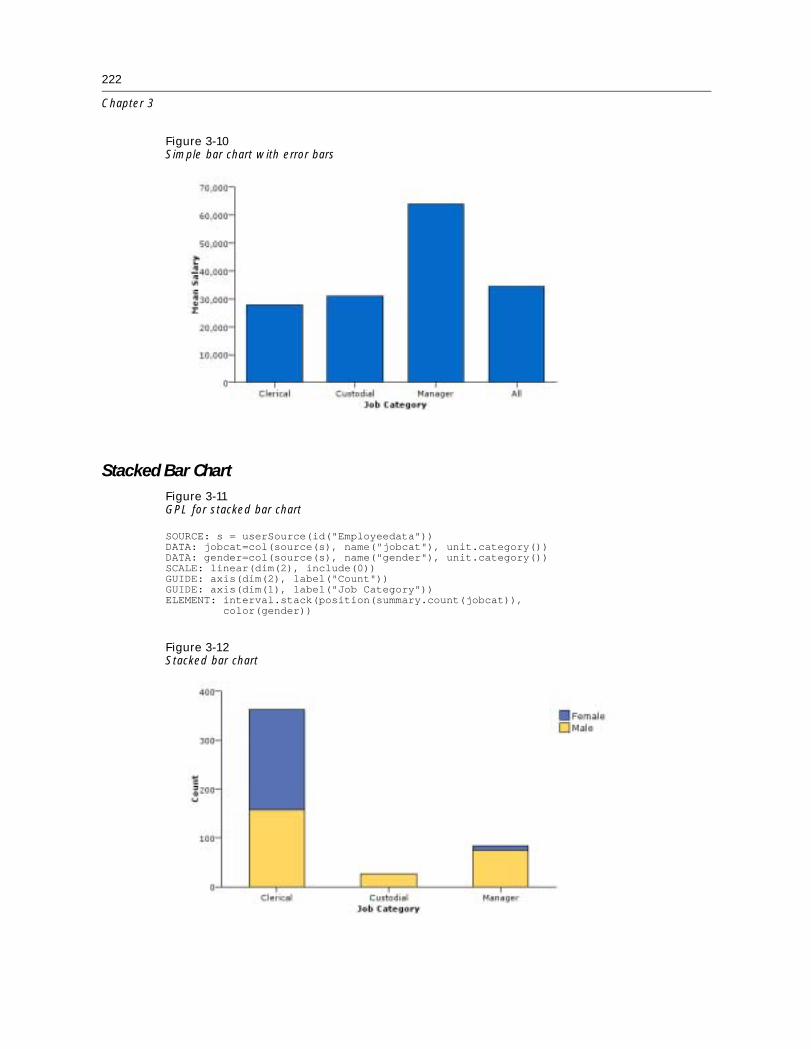
222

Chapter 3

Figure 3-10Simple bar chart with error bars

Stacked Bar ChartFigure 3-11GPL for stacked bar chart

SOURCE: s = userSource(id("Employeedata"))DATA: jobcat=col(source(s), name("jobcat"), unit.category())DATA: gender=col(source(s), name("gender"), unit.category())SCALE: linear(dim(2), include(0))GUIDE: axis(dim(2), label("Count"))GUIDE: axis(dim(1), label("Job Category"))ELEMENT: interval.stack(position(summary.count(jobcat)),

color(gender))

Figure 3-12Stacked bar chart

223

Examples

Clustered Bar ChartFigure 3-13GPL for clustered bar chart



Following is another option for creating a graph that appears clustered. It uses the dodgecollision modiÞer. (See dodge Collision ModiÞer on p. 55.) Note that the difference between thisand the previous example is that empty space is not allocated for missing categories (in this case,the combination of �Female� and �Custodial�).

Figure 3-15GPL for dodged bar chart

SOURCE: s = userSource(id("Employeedata"))DATA: jobcat=col(source(s), name("jobcat"), unit.category())DATA: gender=col(source(s), name("gender"), unit.category())DATA: salary=col(source(s), name("salary"))SCALE: linear(dim(2), include(0))GUIDE: axis(dim(2), label("Mean Salary"))GUIDE: axis(dim(1), label("Gender"))ELEMENT: interval.dodge(position(summary.mean(gender*salary)),

size(size."25%"), color(jobcat))

224

Chapter 3

Figure 3-16Dodged bar chart

Clustered and Stacked Bar ChartFigure 3-17GPL for clustered and stacked bar chart

SOURCE: s = userSource(id("Employeedata"))DATA: jobcat = col(source(s), name("jobcat"), unit.category())DATA: gender = col(source(s), name("gender"), unit.category())DATA: minority = col(source(s), name("minority"), unit.category())DATA: salary = col(source(s), name("salary"))COORD: rect(dim(1, 2), cluster(3, 0))SCALE: linear(dim(2), include(0))GUIDE: axis(dim(2), label("Sum Salary"))GUIDE: axis(dim(3), label("Job Category"))GUIDE: legend(aesthetic(aesthetic.color.interior), label("Gender"))GUIDE: legend(aesthetic(aesthetic.texture.pattern.interior),

label("Minority Classification"))ELEMENT: interval.stack(position(summary.sum(gender*salary*jobcat)),

color.exterior(color.black),color.interior(gender), texture.pattern.interior(minority))

225

Examples

Figure 3-18Clustered and stacked bar chart

Bar Chart Using an Evaluation FunctionFigure 3-19GPL for bar chart using an evaluation function

SOURCE: s = userSource(id("Employeedata"))DATA: salbegin = col(source(s), name("salbegin"))DATA: salary = col(source(s), name("salary"))DATA: jobcat = col(source(s), name("jobcat"), unit.category())DATA: gender = col(source(s), name("gender"), unit.category())TRANS: saldiff = eval(((salary-salbegin)/salary)*100)COORD: rect(dim(1, 2), cluster(3))SCALE: linear(dim(2), include(0))GUIDE: axis(dim(2), label("Mean Percentage Salary Increase"))GUIDE: axis(dim(3), label("Employment Category"))GUIDE: legend(aesthetic(aesthetic.color.interior), label("Gender"))ELEMENT: interval(position(summary.mean(gender*saldiff*jobcat)),

color.interior(gender))

226

Chapter 3

Figure 3-20GPL for bar chart using an evaluation function

Bar Chart with Mapped Aesthetics

This example demonstrates how you can map a speciÞc categorical value in the graph to a speciÞcaesthetic value. In this case, �Female� bars are colored green in the resulting graph.

Figure 3-21GPL for bar chart with mapped aesthetics

SOURCE: s = userSource(id("Employeedata"))DATA: salary = col(source(s), name("salary"))DATA: jobcat = col(source(s), name("jobcat"), unit.category())DATA: gender = col(source(s), name("gender"), unit.category())COORD: rect(dim(1, 2), cluster(3))SCALE: cat(aesthetic(aesthetic.color), map(("f", color.green)))GUIDE: axis(dim(2), label("Mean Salary"))GUIDE: axis(dim(3), label("Job Category"))ELEMENT: interval(position(summary.mean(gender*salary*jobcat)),

color(gender))

227

Examples

Figure 3-22Bar chart with mapped aesthetics

Faceted (Paneled) Bar Chart

Although the following examples create bar charts, faceting is common to all graphs.

Figure 3-23GPL for faceted bar chart

SOURCE: s = userSource(id("Employeedata"))DATA: jobcat = col(source(s), name("jobcat"), unit.category())DATA: gender = col(source(s), name("gender"), unit.category())DATA: salary = col(source(s), name("salary"))SCALE: linear(dim(2), include(0))GUIDE: axis(dim(3), label("Gender"))GUIDE: axis(dim(2), label("Mean Salary"))GUIDE: axis(dim(1), label("Job Category"))ELEMENT: interval(position(summary.mean(jobcat*salary*gender)))

228

Chapter 3


Figure 3-25GPL for faceted bar chart with nested categories

SOURCE: s = userSource(id("Employeedata"))DATA: jobcat = col(source(s), name("jobcat"), unit.category())DATA: gender = col(source(s), name("gender"), unit.category())DATA: salary = col(source(s), name("salary"))SCALE: linear(dim(2), include(0.0))GUIDE: axis(dim(2), label("Mean Salary"))GUIDE: axis(dim(1.1), label("Job Category"))GUIDE: axis(dim(1), label("Gender"))ELEMENT: interval(position(summary.mean(jobcat/gender*salary)))

Figure 3-26Faceted bar chart with nested categories

229

Examples

Figure 3-27GPL for multi-faceted bar chart

SOURCE: s = userSource(id("Employeedata"))DATA: jobcat=col(source(s), name("jobcat"), unit.category())DATA: gender=col(source(s), name("gender"), unit.category())DATA: minority=col(source(s), name("minority"), unit.category())DATA: salary=col(source(s), name("salary"))SCALE: linear(dim(2), include(0))GUIDE: axis(dim(4), label("Minority"))GUIDE: axis(dim(3), label("Gender"))GUIDE: axis(dim(2), label("Mean Salary"))GUIDE: axis(dim(1), label("Job Category"))ELEMENT: interval(position(summary.mean(jobcat*salary*gender*minority)))

Figure 3-28Multi-faceted bar chart

3-D Bar ChartFigure 3-29GPL for 3-D bar chart

SOURCE: s = userSource(id("Employeedata"))DATA: jobcat=col(source(s), name("jobcat"), unit.category())DATA: gender=col(source(s), name("gender"), unit.category())DATA: salary=col(source(s), name("salary"))COORD: rect(dim(1,2,3))SCALE: linear(dim(3), include(0))GUIDE: axis(dim(3), label("Mean Salary"))GUIDE: axis(dim(2), label("Gender"))GUIDE: axis(dim(1), label("Job Category"))ELEMENT: interval(position(summary.mean(jobcat*gender*salary)))

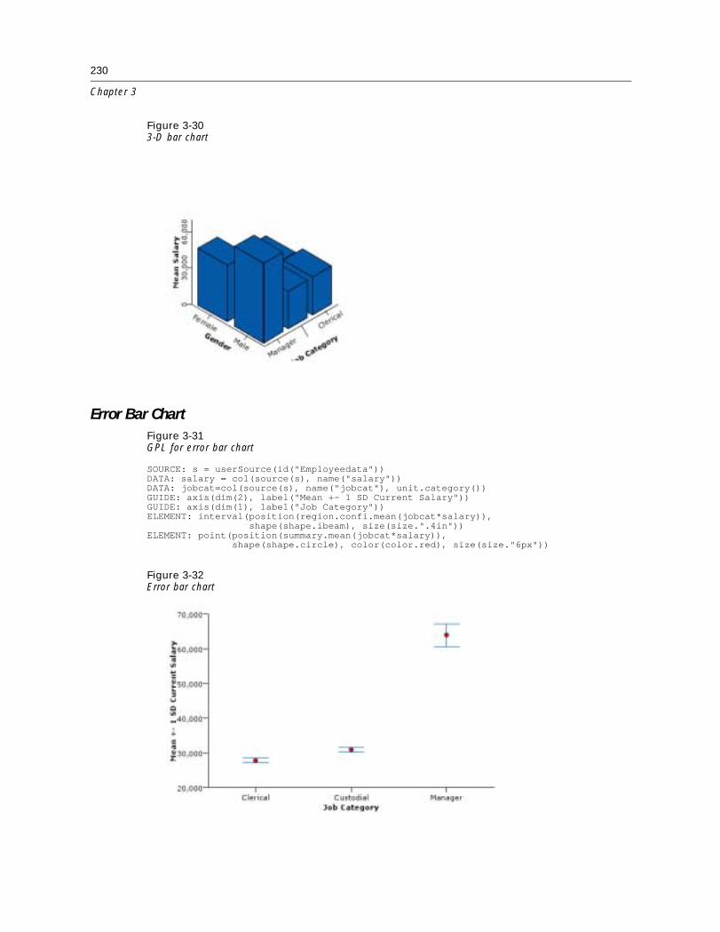
230

Chapter 3

Figure 3-303-D bar chart

Error Bar ChartFigure 3-31GPL for error bar chart

SOURCE: s = userSource(id("Employeedata"))DATA: salary = col(source(s), name("salary"))DATA: jobcat=col(source(s), name("jobcat"), unit.category())GUIDE: axis(dim(2), label("Mean +- 1 SD Current Salary"))GUIDE: axis(dim(1), label("Job Category"))ELEMENT: interval(position(region.confi.mean(jobcat*salary)),

shape(shape.ibeam), size(size.".4in"))ELEMENT: point(position(summary.mean(jobcat*salary)),

shape(shape.circle), color(color.red), size(size."6px"))

Figure 3-32Error bar chart

231

Examples

Histogram Examples

This section provides examples of different types of histograms.

HistogramFigure 3-33GPL for histogram

SOURCE: s = userSource(id("Employeedata"))DATA: salary=col(source(s), name("salary"))GUIDE: axis(dim(2), label("Count"))GUIDE: axis(dim(1), label("Salary"))ELEMENT: interval(position(summary.count(bin.rect(salary))))

Figure 3-34Histogram

Histogram with Distribution CurveFigure 3-35GPL for histogram with normal curve

SOURCE: s = userSource(id("Employeedata"))DATA: salary=col(source(s), name("salary"))GUIDE: axis(dim(2), label("Count"))GUIDE: axis(dim(1), label("Salary"))ELEMENT: interval(position(summary.count(bin.rect(salary))))ELEMENT: line(position(density.normal(salary)))

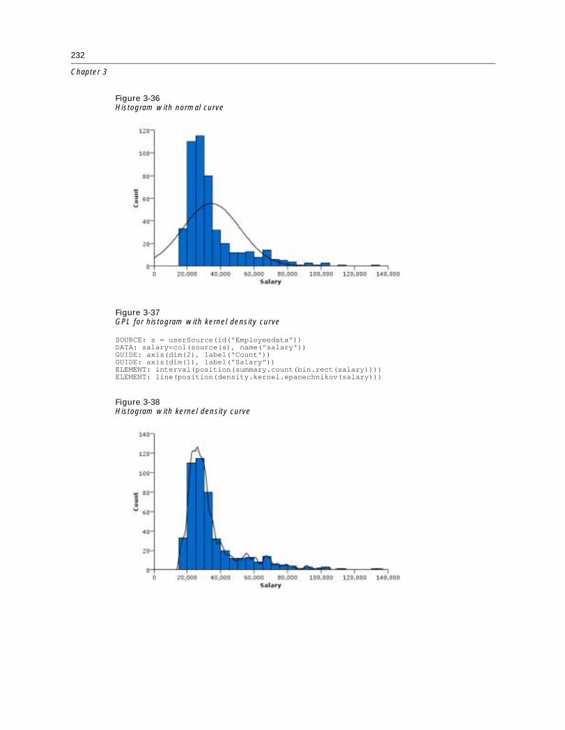
232

Chapter 3

Figure 3-36Histogram with normal curve

Figure 3-37GPL for histogram with kernel density curve

SOURCE: s = userSource(id("Employeedata"))DATA: salary=col(source(s), name("salary"))GUIDE: axis(dim(2), label("Count"))GUIDE: axis(dim(1), label("Salary"))ELEMENT: interval(position(summary.count(bin.rect(salary))))ELEMENT: line(position(density.kernel.epanechnikov(salary)))

Figure 3-38Histogram with kernel density curve

233

Examples

Percentage HistogramFigure 3-39GPL for percentage histogram

SOURCE: s = userSource(id("Employeedata"))DATA: salary = col(source(s), name("salary"))GUIDE: axis(dim(2), label("Percent"))GUIDE: axis(dim(1), label("Salary"))ELEMENT: interval(position(summary.percent.count(bin.rect(salary))))

Figure 3-40Percentage histogram

Frequency PolygonFigure 3-41GPL for frequency polygon

SOURCE: s = userSource(id("Employeedata"))DATA: salary=col(source(s), name("salary"))GUIDE: axis(dim(2), label("Count"))GUIDE: axis(dim(1), label("Salary"))ELEMENT: area(position(summary.count(bin.rect(salary))))

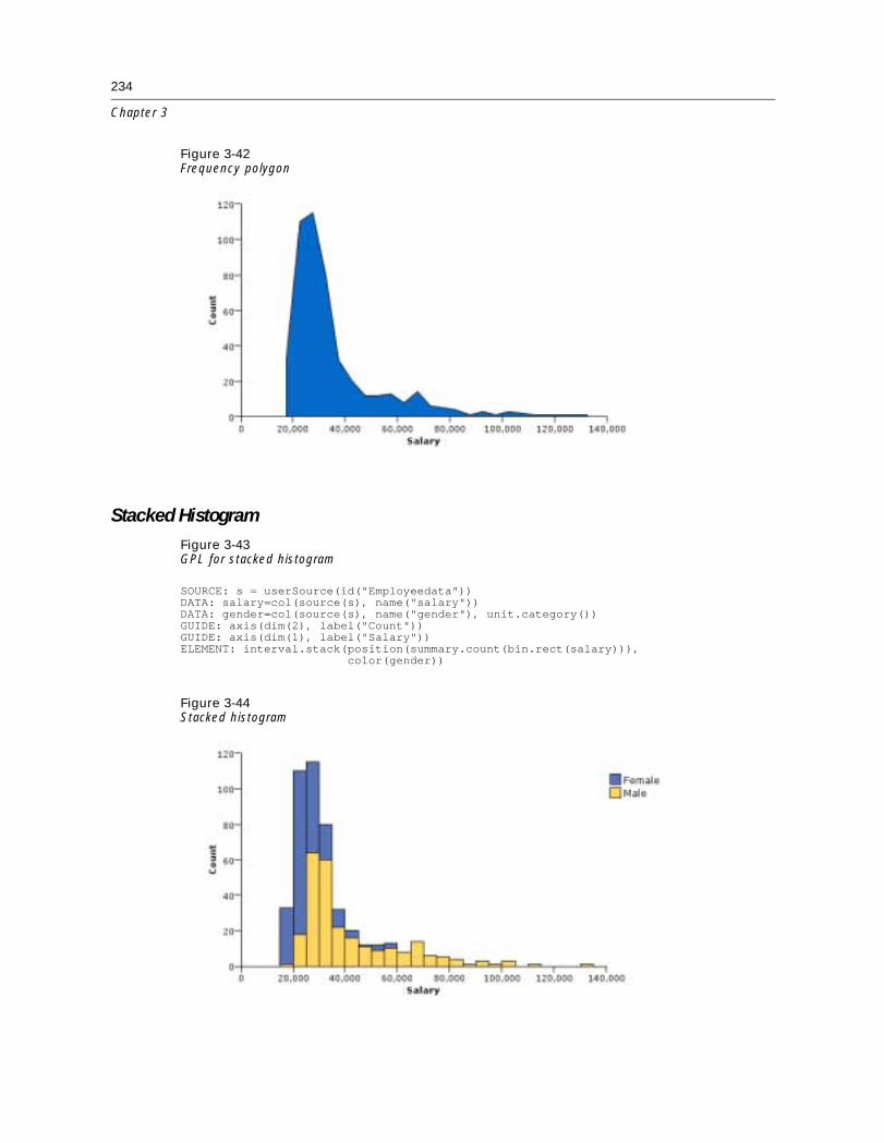
234

Chapter 3

Figure 3-42Frequency polygon

Stacked HistogramFigure 3-43GPL for stacked histogram

SOURCE: s = userSource(id("Employeedata"))DATA: salary=col(source(s), name("salary"))DATA: gender=col(source(s), name("gender"), unit.category())GUIDE: axis(dim(2), label("Count"))GUIDE: axis(dim(1), label("Salary"))ELEMENT: interval.stack(position(summary.count(bin.rect(salary))),

color(gender))

Figure 3-44Stacked histogram

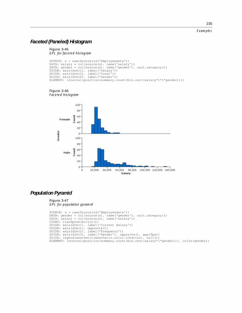
235

Examples

Faceted (Paneled) HistogramFigure 3-45GPL for faceted histogram

SOURCE: s = userSource(id("Employeedata"))DATA: salary = col(source(s), name("salary"))DATA: gender = col(source(s), name("gender"), unit.category())GUIDE: axis(dim(1), label("Salary"))GUIDE: axis(dim(2), label("Count"))GUIDE: axis(dim(4), label("Gender"))ELEMENT: interval(position(summary.count(bin.rect(salary*1*1*gender))))

Figure 3-46Faceted histogram

Population PyramidFigure 3-47GPL for population pyramid

SOURCE: s = userSource(id("Employeedata"))DATA: gender = col(source(s), name("gender"), unit.category())DATA: salary = col(source(s), name("salary"))COORD: transpose(mirror())GUIDE: axis(dim(1), label("Current Salary"))GUIDE: axis(dim(1), opposite())GUIDE: axis(dim(2), label("Frequency"))GUIDE: axis(dim(3), label("Gender"), opposite(), gap(0px))GUIDE: legend(aesthetic(aesthetic.color.interior), null())ELEMENT: interval(position(summary.count(bin.rect(salary*1*gender))), color(gender))

236

Chapter 3

Figure 3-48Population pyramid

Cumulative Histogram

Figure 3-49GPL for cumulative histogram

SOURCE: s = userSource(id("Employeedata"))DATA: salary=col(source(s), name("salary"))GUIDE: axis(dim(2), label("Cumulative Percent"))GUIDE: axis(dim(1), label("Salary"))ELEMENT: interval(position(summary.percent.count.cumulative(bin.rect(salary))))

Figure 3-50Cumulative histogram

237

Examples

3-D Histogram

Figure 3-51GPL for 3-D histogram

SOURCE: s = userSource(id("Employeedata"))DATA: salary = col(source(s), name("salary"))DATA: jobcat = col(source(s), name("jobcat"), unit.category())COORD: rect(dim(1, 2, 3))GUIDE: axis(dim(1), label("Employment Category"))GUIDE: axis(dim(2), label("Salary"))GUIDE: axis(dim(3), label("Count"))ELEMENT: interval(position(summary.count(bin.rect(jobcat*salary, dim(2)))))

Figure 3-523-D histogram

High-Low Chart Examples

This section provides examples of different types of high-low charts.

Simple Range Bar for One Variable

Figure 3-53GPL for simple range bar for one variable

SOURCE: s = userSource(id("Employeedata"))DATA: jobcat=col(source(s), name("jobcat"), unit.category())DATA: salary=col(source(s), name("salary"))SCALE: linear(dim(2), min(0.0))GUIDE: axis(dim(2), label("Min Current Salary - Max Current Salary"))GUIDE: axis(dim(1), label("Job Category"))ELEMENT: interval(position(region.spread.range(jobcat*salary)))

238

Chapter 3

Figure 3-54Simple range bar for one variable

Simple Range Bar for Two VariablesFigure 3-55GPL for simple range bar for two variables

SOURCE: s = userSource(id("Employeedata"))DATA: jobcat=col(source(s), name("jobcat"), unit.category())DATA: salbegin=col(source(s), name("salbegin"))DATA: salary=col(source(s), name("salary"))SCALE: linear(dim(2), min(0.0))GUIDE: axis(dim(2), label("Min Beginning Salary - Max Current Salary"))GUIDE: axis(dim(1), label("Job Category"))ELEMENT: interval(position(region.spread.range(jobcat*(salbegin+salary))))

Figure 3-56Simple range bar for two variables

239

Examples

High-Low-Close ChartFigure 3-57GPL for high-low-close chart

SOURCE: s = userSource(id("stocks2004"))DATA: Date = col(source(s), name("Date"), unit.time(), format("MM/dd/yy"))DATA: Close = col(source(s), name("Close"))DATA: High = col(source(s), name("High"))DATA: Low = col(source(s), name("Low"))GUIDE: text.title(label("NASDAQ Composite"))GUIDE: axis(dim(1), label("Date"))GUIDE: axis(dim(2), label("Close"))SCALE: time(dim(1), dataMaximum())ELEMENT: interval(position(region.spread.range(Date*(Low+High))))ELEMENT: point(position(Date*Close), color.exterior(color.red), size(size."2px"))

Figure 3-58High-low-close chart

Difference Area ChartFigure 3-59GPL for difference area chart

SOURCE: s = userSource(id("Employeedata"))DATA: jobcat = col(source(s), name("jobcat"), unit.category())DATA: gender = col(source(s), name("gender"), unit.category())SCALE: linear(dim(2), include(0.0))GUIDE: axis(dim(2), label("Count"))GUIDE: axis(dim(1), label("Job Category"))ELEMENT: area.difference(position(summary.count(jobcat)), color(gender))

240

Chapter 3

Figure 3-60Difference area chart

Scatter/Dot Examples

This section provides examples of different types of scatterplots and dot plots.

Simple 1-D ScatterplotFigure 3-61GPL for simple 1-D scatterplot

SOURCE: s = userSource(id("Employeedata"))DATA: salary = col(source(s), name("salary"))COORD: rect(dim(1))GUIDE: axis(dim(1), label("Salary"))ELEMENT: point(position(salary))

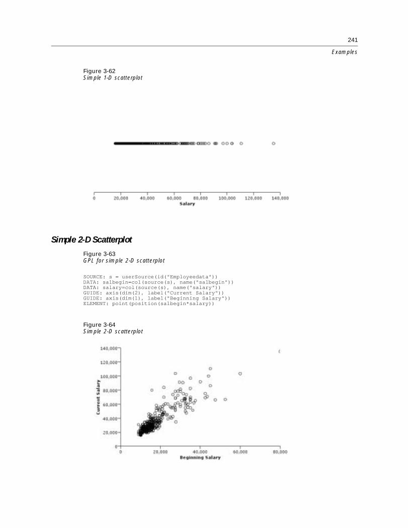
241

Examples


Simple 2-D Scatterplot

Figure 3-63GPL for simple 2-D scatterplot



242

Chapter 3

Simple 2-D Scatterplot with Fit LineFigure 3-65GPL for simple scatterplot with fit line

SOURCE: s = userSource(id("Employeedata"))DATA: salbegin=col(source(s), name("salbegin"))DATA: salary=col(source(s), name("salary"))GUIDE: axis(dim(2), label("Current Salary"))GUIDE: axis(dim(1), label("Beginning Salary"))ELEMENT: point(position(salbegin*salary))ELEMENT: line(position(smooth.linear(salbegin*salary)))

Figure 3-66Simple scatterplot with fit line

Grouped ScatterplotFigure 3-67GPL for grouped scatterplot

SOURCE: s = userSource(id("Employeedata"))DATA: salbegin=col(source(s), name("salbegin"))DATA: salary=col(source(s), name("salary"))DATA: gender=col(source(s), name("gender"), unit.category())GUIDE: axis(dim(2), label("Current Salary"))GUIDE: axis(dim(1), label("Beginning Salary"))ELEMENT: point(position(salbegin*salary), color(gender))

243

Examples

Figure 3-68Grouped scatterplot

Grouped Scatterplot with Convex HullFigure 3-69GPL for grouped scatterplot with convex hull

SOURCE: s = userSource(id("Employeedata"))DATA: salbegin=col(source(s), name("salbegin"))DATA: salary=col(source(s), name("salary"))DATA: gender=col(source(s), name("gender"), unit.category())GUIDE: axis(dim(1), label("Beginning Salary"))GUIDE: axis(dim(2), label("Current Salary"))GUIDE: legend(aesthetic(aesthetic.color.exterior), label("Gender"))GUIDE: legend(aesthetic(aesthetic.color.interior), null())ELEMENT: point(position(salbegin*salary), color.exterior(gender))ELEMENT: edge(position(link.hull(salbegin*salary)), color.interior(gender))

244

Chapter 3

Figure 3-70Grouped scatterplot with convex hull

Scatterplot Matrix (SPLOM)Figure 3-71GPL for scatterplot matrix

SOURCE: s = userSource(id("Cars"))DATA: weight=col(source(s), name("weight"))DATA: mpg=col(source(s), name("mpg"))DATA: horse=col(source(s), name("horse"))GUIDE: axis(dim(1.1), ticks(null()))GUIDE: axis(dim(2.1), ticks(null()))GUIDE: axis(dim(1), gap(0px))GUIDE: axis(dim(2), gap(0px))ELEMENT: point(position((mpg/"MPG"+weight/"Weight"+horse/"HP")*

(mpg/"MPG"+weight/"Weight"+horse/"HP")))

245

Examples

Figure 3-72Scatterplot Matrix

Bubble PlotFigure 3-73GPL for bubble plot

SOURCE: s = userSource(id("Employeedata"))DATA: salbegin=col(source(s), name("salbegin"))DATA: salary=col(source(s), name("salary"))DATA: prevexp=col(source(s), name("prevexp"))SCALE: linear(aesthetic(aesthetic.size),

aestheticMinimum(size."5px"), aestheticMaximum(size."35px"))GUIDE: axis(dim(2), label("Current Salary"))GUIDE: axis(dim(1), label("Beginning Salary"))GUIDE: legend(aesthetic(aesthetic.size), label("Previous Experience (months)"))ELEMENT: point(position(salbegin*salary), size(prevexp))

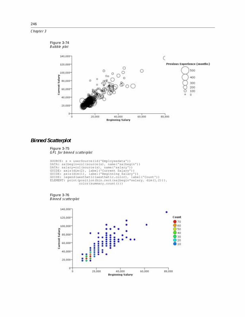
246

Chapter 3

Figure 3-74Bubble plot

Binned ScatterplotFigure 3-75GPL for binned scatterplot

SOURCE: s = userSource(id("Employeedata"))DATA: salbegin=col(source(s), name("salbegin"))DATA: salary=col(source(s), name("salary"))GUIDE: axis(dim(2), label("Current Salary"))GUIDE: axis(dim(1), label("Beginning Salary"))GUIDE: legend(aesthetic(aesthetic.color), label("Count"))ELEMENT: point(position(bin.rect(salbegin*salary, dim(1,2))),

color(summary.count()))

Figure 3-76Binned scatterplot

247

Examples

Binned Scatterplot with PolygonsFigure 3-77GPL for binned scatterplot with polygons

SOURCE: s = userSource(id("Employeedata"))DATA: salbegin=col(source(s), name("salbegin"))DATA: salary=col(source(s), name("salary"))GUIDE: axis(dim(2), label("Current Salary"))GUIDE: axis(dim(1), label("Beginning Salary"))GUIDE: legend(aesthetic(aesthetic.color), label("Count"))ELEMENT: polygon(position(bin.hex(salbegin*salary, dim(1,2))),

color(summary.count()))

Figure 3-78Binned scatterplot with polygons

Scatterplot with Border HistogramsFigure 3-79GPL for scatterplot with border histograms

SOURCE: s = userSource(id("Employeedata"))DATA: salary = col(source(s), name("salary"))DATA: salbegin = col(source(s), name("salbegin"))GRAPH: begin(origin(5%, 10%), scale(85%, 85%))GUIDE: axis(dim(1), label("Beginning Salary"))GUIDE: axis(dim(2), label("Current Salary"))ELEMENT: point(position(salbegin*salary))GRAPH: end()GRAPH: begin(origin(5%, 0%), scale(85%, 10%))GUIDE: axis(dim(1), ticks(null()))GUIDE: axis(dim(2), null())ELEMENT: interval(position(summary.count(bin.rect(salbegin))))GRAPH: end()GRAPH: begin(origin(90%, 10%), scale(10%, 85%))COORD: rect(dim(1, 2), transpose())GUIDE: axis(dim(1), ticks(null()))GUIDE: axis(dim(2), null())ELEMENT: interval(position(summary.count(bin.rect(salary))))GRAPH: end()

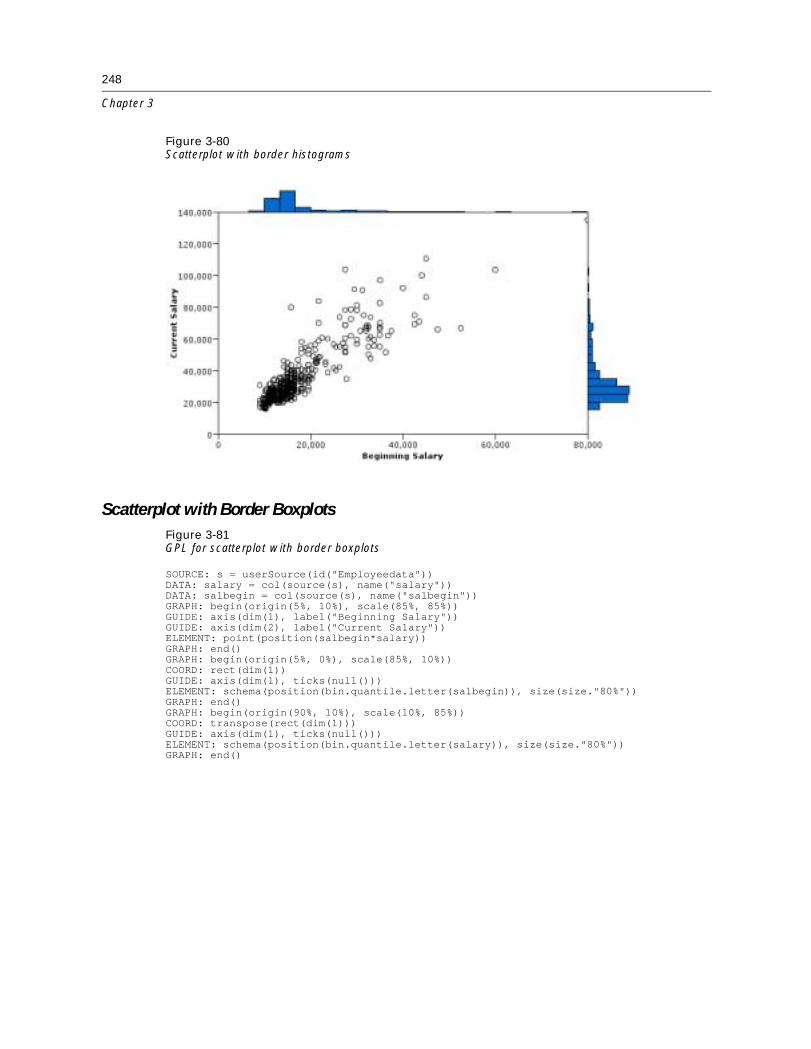
248

Chapter 3

Figure 3-80Scatterplot with border histograms

Scatterplot with Border BoxplotsFigure 3-81GPL for scatterplot with border boxplots

SOURCE: s = userSource(id("Employeedata"))DATA: salary = col(source(s), name("salary"))DATA: salbegin = col(source(s), name("salbegin"))GRAPH: begin(origin(5%, 10%), scale(85%, 85%))GUIDE: axis(dim(1), label("Beginning Salary"))GUIDE: axis(dim(2), label("Current Salary"))ELEMENT: point(position(salbegin*salary))GRAPH: end()GRAPH: begin(origin(5%, 0%), scale(85%, 10%))COORD: rect(dim(1))GUIDE: axis(dim(1), ticks(null()))ELEMENT: schema(position(bin.quantile.letter(salbegin)), size(size."80%"))GRAPH: end()GRAPH: begin(origin(90%, 10%), scale(10%, 85%))COORD: transpose(rect(dim(1)))GUIDE: axis(dim(1), ticks(null()))ELEMENT: schema(position(bin.quantile.letter(salary)), size(size."80%"))GRAPH: end()

249

Examples

Figure 3-82Scatterplot with border boxplots

Dot PlotFigure 3-83GPL for dot plot

SOURCE: s = userSource(id("Employeedata"))DATA: salary = col(source(s), name("salary"))COORD: rect(dim(1))GUIDE: axis(dim(1), label("Salary"))ELEMENT: point.dodge.asymmetric(position(bin.dot(salary)))

Figure 3-84Dot plot

250

Chapter 3

Figure 3-85GPL for grouped dot plot

SOURCE: s = userSource(id("Employeedata"))DATA: gender = col(source(s), name("gender"), unit.category())DATA: salary = col(source(s), name("salary"))GUIDE: axis(dim(1), label("Salary"))COORD: rect(dim(1))ELEMENT: point.dodge.asymmetric(position(bin.dot(salary)),

color(gender), shape(shape.square))

Figure 3-86Grouped dot plot

2-D Dot PlotFigure 3-87GPL for 2-D dot plot

SOURCE: s = userSource(id("Cars"))DATA: origin = col(source(s), name("origin"), unit.category())DATA: mpg = col(source(s), name("mpg"))GUIDE: axis(dim(1), label("Miles Per Gallon"), delta(5.0))GUIDE: axis(dim(2), label("Country of Origin"))ELEMENT: point.dodge.symmetric(position(bin.dot(mpg*origin)))

251

Examples

Figure 3-882-D dot plot

Figure 3-89GPL for alternate 2-D dot plot

SOURCE: s = userSource(id("Cars"))DATA: origin = col(source(s), name("origin"), unit.category())DATA: mpg = col(source(s), name("mpg"))GUIDE: axis(dim(1), label("Miles Per Gallon"), delta(5.0))GUIDE: axis(dim(2), label("Country of Origin"))ELEMENT: point.dodge.symmetric(position(bin.dot(origin*mpg, dim(2))))

Figure 3-90Alternate 2-D dot plot

252

Chapter 3

Jittered Categorical ScatterplotFigure 3-91GPL for jittered categorical scatterplot

SOURCE: s = userSource(id("Employeedata"))DATA: jobcat=col(source(s), name("jobcat"), unit.category())DATA: gender=col(source(s), name("gender"), unit.category())GUIDE: axis(dim(2), label("Gender"))GUIDE: axis(dim(1), label("Employment Category"))ELEMENT: point.jitter(position(jobcat*gender))

Figure 3-92Jittered categorical scatterplot

Line Chart Examples

This section provides examples of different types of line charts.

Simple Line ChartFigure 3-93GPL for simple line chart

SOURCE: s = userSource(id("Employeedata"))DATA: salbegin=col(source(s), name("salbegin"))DATA: salary=col(source(s), name("salary"))GUIDE: axis(dim(2), label("Current Salary"))GUIDE: axis(dim(1), label("Beginning Salary"))ELEMENT: line(position(salbegin*salary))

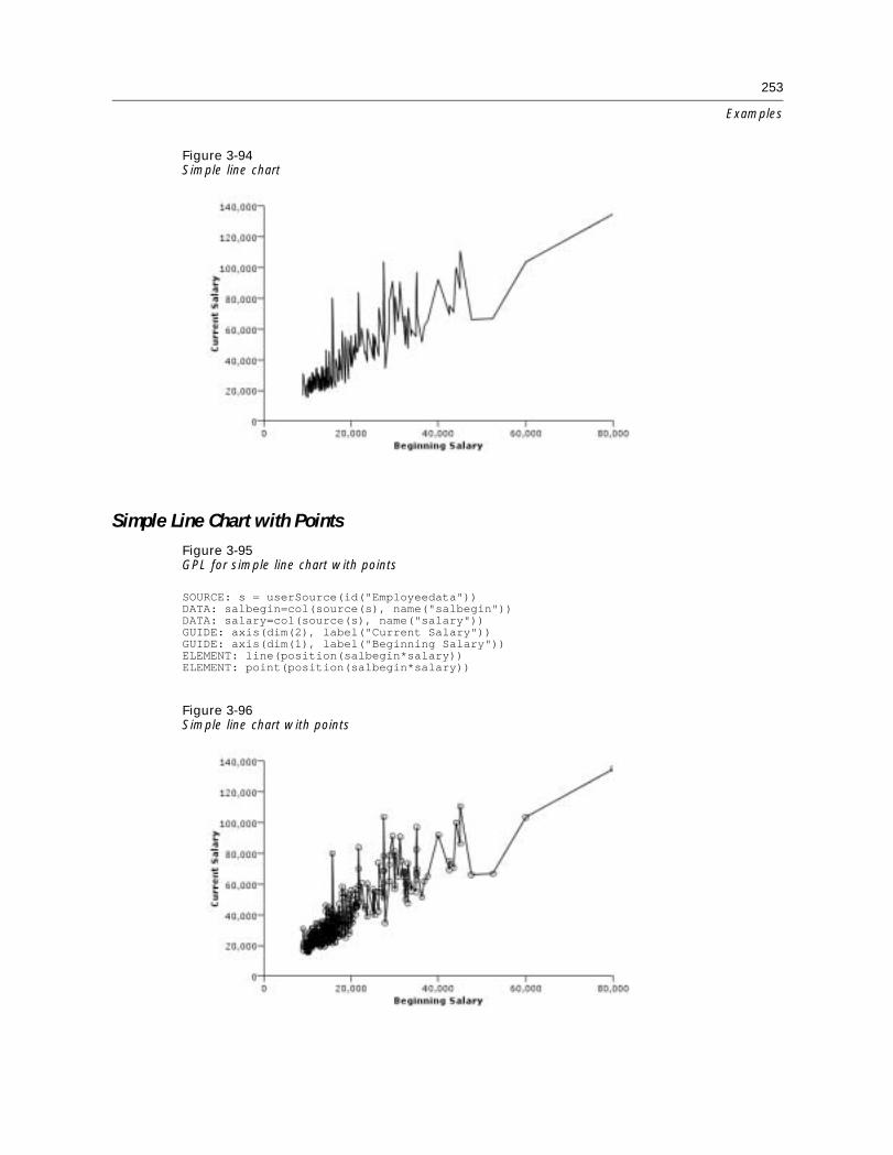
253

Examples

Figure 3-94Simple line chart

Simple Line Chart with PointsFigure 3-95GPL for simple line chart with points

SOURCE: s = userSource(id("Employeedata"))DATA: salbegin=col(source(s), name("salbegin"))DATA: salary=col(source(s), name("salary"))GUIDE: axis(dim(2), label("Current Salary"))GUIDE: axis(dim(1), label("Beginning Salary"))ELEMENT: line(position(salbegin*salary))ELEMENT: point(position(salbegin*salary))

Figure 3-96Simple line chart with points

254

Chapter 3

Line Chart of Date DataFigure 3-97GPL for line chart of date data

SOURCE: s = userSource(id("stocks2004"))DATA: Date = col(source(s), name("Date"), unit.time(), format("MM/dd/yy"))DATA: Close = col(source(s), name("Close"))GUIDE: text.title(label("NASDAQ Composite"))GUIDE: axis(dim(1), label("Date"))GUIDE: axis(dim(2), label("Close"))SCALE: time(dim(1), dataMaximum())ELEMENT: line(position(Date*Close))

Figure 3-98Line chart of date data

Line Chart With Step InterpolationFigure 3-99GPL for line chart with step interpolation

SOURCE: s = userSource(id("Employeedata"))DATA: salbegin=col(source(s), name("salbegin"))DATA: salary=col(source(s), name("salary"))GUIDE: axis(dim(2), label("Current Salary"))GUIDE: axis(dim(1), label("Beginning Salary"))ELEMENT: line(position(smooth.step.center(salbegin*salary)))

255

Examples

Figure 3-100Line chart with step interpolation

Fit LineFigure 3-101GPL for linear fit line overlaid on scatterplot

SOURCE: s = userSource(id("Employeedata"))DATA: salbegin=col(source(s), name("salbegin"))DATA: salary=col(source(s), name("salary"))GUIDE: axis(dim(2), label("Current Salary"))GUIDE: axis(dim(1), label("Beginning Salary"))ELEMENT: point(position(salbegin*salary))ELEMENT: line(position(smooth.linear(salbegin*salary)))

Figure 3-102Linear fit line overlaid on scatterplot

256

Chapter 3

Line Chart from EquationFigure 3-103GPL for line chart from equation

DATA: x = iter(0,10,0.01)TRANS: y = eval(sin(x)*cos(x)*(x-5))ELEMENT: line(position(x*y))

Figure 3-104Line chart from equation

Figure 3-105GPL for line chart from equation in polar coordinates

DATA: x = iter(0,6.28,0.01)TRANS: y = eval(cos(6*x))COORD: polar()SCALE: linear(dim(1), min(0.0), max(6.28))GUIDE: axis(dim(2), null())ELEMENT: line(position(x*y))

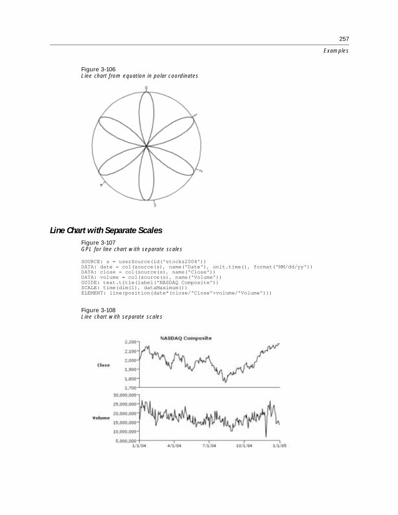
257

Examples

Figure 3-106Line chart from equation in polar coordinates

Line Chart with Separate ScalesFigure 3-107GPL for line chart with separate scales

SOURCE: s = userSource(id("stocks2004"))DATA: date = col(source(s), name("Date"), unit.time(), format("MM/dd/yy"))DATA: close = col(source(s), name("Close"))DATA: volume = col(source(s), name("Volume"))GUIDE: text.title(label("NASDAQ Composite"))SCALE: time(dim(1), dataMaximum())ELEMENT: line(position(date*(close/"Close"+volume/"Volume")))

Figure 3-108Line chart with separate scales

258

Chapter 3

Line Chart in Parallel Coordinates

The following example creates a line chart in parallel coordinates. If we didn�t use the result ofthe index function to split the line, every case would be connected, so there would be only oneline in the resulting graph. The line would appear to zigzag back and forth between the last axisand the Þrst one. The explicit transparency setting is not required. It is used so that it is easier toread the axis labels.

Figure 3-109GPL for line chart in parallel coordinates

SOURCE: s = userSource(id("World95"))DATA: lifeexpm=col(source(s), name("lifeexpm"))DATA: lifeexpf=col(source(s), name("lifeexpf"))DATA: babymort=col(source(s), name("babymort"))DATA: literacy=col(source(s), name("literacy"))DATA: region=col(source(s), name("region"), unit.category())TRANS: caseid = index()COORD: parallel()GUIDE: axis(dim(1), label("Life Expectancy (Males)"))GUIDE: axis(dim(2), label("Life Expectancy (Females)"))GUIDE: axis(dim(3), label("Literacy"))GUIDE: axis(dim(4), label("Infant Mortality"))GUIDE: legend(aesthetic(aesthetic.color), label("Region"))ELEMENT: line(position(lifeexpm*lifeexpf*literacy*babymort),

split(caseid), color(region),transparency(transparency."0.5"))

Figure 3-110Line chart in parallel coordinates

Here is the same chart plotted in polar coordinates. We also reversed the scale for dimension 4to emphasize the relationship among the variables. As you can see, there are distinct bands ofcolor representing the different regions. Also note the preserveStraightLines and closedfunctions, which improve the look of the graph in polar coordinates.

259

Examples

Figure 3-111GPL for line chart in polar parallel coordinates

SOURCE: s = userSource(id("World95"))DATA: lifeexpm=col(source(s), name("lifeexpm"))DATA: lifeexpf=col(source(s), name("lifeexpf"))DATA: babymort=col(source(s), name("babymort"))DATA: literacy=col(source(s), name("literacy"))DATA: region=col(source(s), name("region"), unit.category())TRANS: caseid = index()COORD: polar(parallel())SCALE: linear(dim(4), reverse())GUIDE: axis(dim(1), label("Life Expectancy (Males)"))GUIDE: axis(dim(2), label("Life Expectancy (Females)"))GUIDE: axis(dim(3), label("Literacy"))GUIDE: axis(dim(4), label("Infant Mortality"))GUIDE: legend(aesthetic(aesthetic.color), label("Region"))ELEMENT: line(position(lifeexpm*lifeexpf*literacy*babymort),

split(caseid), color(region),transparency(transparency."0.5"),preserveStraightLines(), closed())

Figure 3-112Line chart in polar parallel coordinates

Pie Chart Examples

This section provides examples of different types of pie charts.

Pie ChartFigure 3-113GPL for pie chart

SOURCE: s = userSource(id("Employeedata"))DATA: jobcat=col(source(s), name("jobcat"), unit.category())COORD: polar.theta()SCALE: linear(dim(1), dataMinimum(), dataMaximum())GUIDE: axis(dim(1), null())ELEMENT: interval.stack(position(summary.count()), color(jobcat))

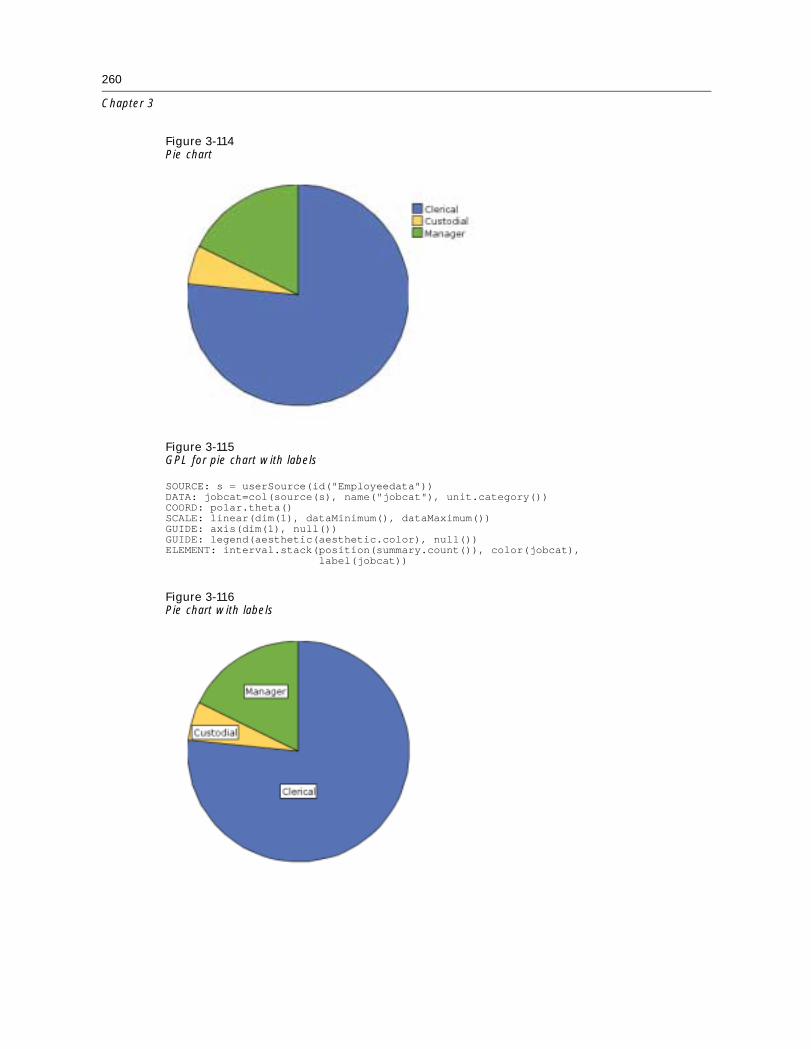
260

Chapter 3

Figure 3-114Pie chart

Figure 3-115GPL for pie chart with labels

SOURCE: s = userSource(id("Employeedata"))DATA: jobcat=col(source(s), name("jobcat"), unit.category())COORD: polar.theta()SCALE: linear(dim(1), dataMinimum(), dataMaximum())GUIDE: axis(dim(1), null())GUIDE: legend(aesthetic(aesthetic.color), null())ELEMENT: interval.stack(position(summary.count()), color(jobcat),

label(jobcat))

Figure 3-116Pie chart with labels

261

Examples

Paneled Pie ChartFigure 3-117GPL for paneled pie chart

SOURCE: s = userSource(id("Employeedata"))DATA: jobcat = col(source(s), name("jobcat"), unit.category())DATA: gender = col(source(s), name("gender"), unit.category())COORD: polar.theta()SCALE: linear(dim(1), dataMinimum(), dataMaximum())GUIDE: axis(dim(1), null())GUIDE: axis(dim(2), label("Gender"))ELEMENT: interval.stack(position(summary.percent.count(1*gender))),

color(jobcat))

Figure 3-118Paneled pie chart

Boxplot Examples

This section provides examples of different types of box plots.

1-D BoxplotFigure 3-119GPL for 1-D box plot

SOURCE: s = userSource(id("Employeedata"))DATA: salary = col(source(s), name("salary"))COORD: rect(dim(1))GUIDE: axis(dim(1), label("Salary"))ELEMENT: schema(position(bin.quantile.letter(salary)), size(size."50%"))

262

Chapter 3

Figure 3-1201-D boxplot

Boxplot

Figure 3-121GPL for boxplot

SOURCE: s = userSource(id("Employeedata"))DATA: jobcat=col(source(s), name("jobcat"), unit.category())DATA: salary=col(source(s), name("salary"))GUIDE: axis(dim(2), label("Salary"))GUIDE: axis(dim(1), label("Job Category"))ELEMENT: schema(position(bin.quantile.letter(jobcat*salary)))

Figure 3-122Boxplot

263

Examples

Figure 3-123GPL for boxplot with labeled outliers

SOURCE: s = userSource(id("Employeedata"))DATA: jobcat=col(source(s), name("jobcat"), unit.category())DATA: salary=col(source(s), name("salary"))DATA: id = col(source(s), name("id"), unit.category())GUIDE: axis(dim(2), label("Salary"))GUIDE: axis(dim(1), label("Job Category"))ELEMENT: schema(position(bin.quantile.letter(jobcat*salary)), label(id))

Figure 3-124Boxplot with labeled outliers

Clustered BoxplotFigure 3-125GPL for clustered boxplot

SOURCE: s = userSource(id("Employeedata"))DATA: jobcat=col(source(s), name("jobcat"), unit.category())DATA: gender=col(source(s), name("gender"), unit.category())DATA: salary=col(source(s), name("salary"))COORD: rect(dim(1,2), cluster(3))GUIDE: axis(dim(2), label("Salary"))GUIDE: axis(dim(3), label("Job Category"))ELEMENT: schema(position(bin.quantile.letter(gender*salary*jobcat)), color(gender))

264

Chapter 3

Figure 3-126Clustered boxplot

Boxplot With Overlaid Dot PlotFigure 3-127GPL for boxplot with overlaid dot plot

SOURCE: s = userSource(id("World95"))DATA: region = col(source(s), name("region"), unit.category())DATA: birth = col(source(s), name("birth_rt"))GUIDE: axis(dim(2), label("Birth Rate"))GUIDE: axis(dim(1), label("Region"))SCALE: linear(dim(2), include(0))ELEMENT: schema(position(bin.quantile.letter(region*birth)))ELEMENT: point.dodge.symmetric(position(bin.dot(region*birth, dim(2))),

color(color.red))

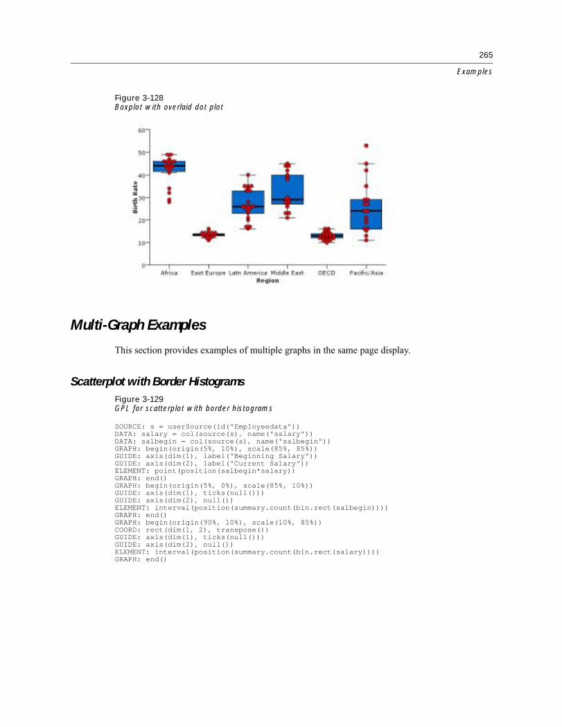
265

Examples

Figure 3-128Boxplot with overlaid dot plot

Multi-Graph Examples

This section provides examples of multiple graphs in the same page display.

Scatterplot with Border HistogramsFigure 3-129GPL for scatterplot with border histograms

SOURCE: s = userSource(id("Employeedata"))DATA: salary = col(source(s), name("salary"))DATA: salbegin = col(source(s), name("salbegin"))GRAPH: begin(origin(5%, 10%), scale(85%, 85%))GUIDE: axis(dim(1), label("Beginning Salary"))GUIDE: axis(dim(2), label("Current Salary"))ELEMENT: point(position(salbegin*salary))GRAPH: end()GRAPH: begin(origin(5%, 0%), scale(85%, 10%))GUIDE: axis(dim(1), ticks(null()))GUIDE: axis(dim(2), null())ELEMENT: interval(position(summary.count(bin.rect(salbegin))))GRAPH: end()GRAPH: begin(origin(90%, 10%), scale(10%, 85%))COORD: rect(dim(1, 2), transpose())GUIDE: axis(dim(1), ticks(null()))GUIDE: axis(dim(2), null())ELEMENT: interval(position(summary.count(bin.rect(salary))))GRAPH: end()

266

Chapter 3

Figure 3-130Scatterplot with border histograms

Scatterplot with Border BoxplotsFigure 3-131GPL for scatterplot with border boxplots

SOURCE: s = userSource(id("Employeedata"))DATA: salary = col(source(s), name("salary"))DATA: salbegin = col(source(s), name("salbegin"))GRAPH: begin(origin(5%, 10%), scale(85%, 85%))GUIDE: axis(dim(1), label("Beginning Salary"))GUIDE: axis(dim(2), label("Current Salary"))ELEMENT: point(position(salbegin*salary))GRAPH: end()GRAPH: begin(origin(5%, 0%), scale(85%, 10%))COORD: rect(dim(1))GUIDE: axis(dim(1), ticks(null()))ELEMENT: schema(position(bin.quantile.letter(salbegin)), size(size."80%"))GRAPH: end()GRAPH: begin(origin(90%, 10%), scale(10%, 85%))COORD: transpose(rect(dim(1)))GUIDE: axis(dim(1), ticks(null()))ELEMENT: schema(position(bin.quantile.letter(salary)), size(size."80%"))GRAPH: end()

267

Examples

Figure 3-132Scatterplot with border boxplots

Stocks Line Chart with Volume Bar ChartFigure 3-133GPL for stocks and volume chart

SOURCE: s = userSource(id("stocks2004"))DATA: date = col(source(s), name("Date"), unit.time(), format("MM/dd/yy"))DATA: close = col(source(s), name("Close"))DATA: volume = col(source(s), name("Volume"))GRAPH: begin(origin(5%, 0%), scale(90%, 60%))GUIDE: axis(dim(1), ticks(null()))GUIDE: axis(dim(2), label("Close"))ELEMENT: line(position(date*close)))GRAPH: end()GRAPH: begin(origin(5%, 70%), scale(90%, 25%))GUIDE: axis(dim(1), label("Date"))GUIDE: axis(dim(2), label("Volume"))ELEMENT: interval(position(date*volume))GRAPH: end()

268

Chapter 3

Figure 3-134Stocks and volume chart

Dual Axis GraphFigure 3-135GPL for dual axis graph

SOURCE: s = userSource(id("Employeedata"))DATA: jobcat = col(source(s), name("jobcat"), unit.category())DATA: salary = col(source(s), name("salary"))SCALE: y1 = linear(dim(2), include(0.0))SCALE: y2 = linear(dim(2), include(0.0))GUIDE: axis(dim(1), label("Employment Category"))GUIDE: axis(scale(y1), label("Mean Salary"))GUIDE: axis(scale(y2), label("Count"), opposite(), color(color.red))ELEMENT: interval(position(summary.mean(jobcat*salary)), scale(y1))ELEMENT: line(position(summary.count(jobcat)), color(color.red), scale(y2))

269

Examples

Figure 3-136Dual axis graph

Histogram with Dot PlotFigure 3-137GPL for histogram with dot plot

SOURCE: s = userSource(id("Employeedata"))DATA: salary = col(source(s), name("salary"))GRAPH: begin(origin(5.0%, 5.0%), scale(90.0%, 90.0%))COORD: rect(dim(1, 2))ELEMENT: interval(position(summary.count(bin.rect(salary))),

transparency.interior(transparency."0.9"))GRAPH: end()GRAPH: begin(origin(5.0%, 5.0%), scale(90.0%, 90.0%))COORD: rect(dim(1))GUIDE: axis(dim(1), ticks(null()))GUIDE: axis(dim(2), ticks(null()))ELEMENT: point.dodge.asymmetric(position(bin.dot(salary)))GRAPH: end()

270

Chapter 3

Figure 3-138Histogram with dot plot

Other Examples

This section provides examples that demonstrate other features of GPL that are not speciÞcto chart types.

Collapsing Small Categories

If you are creating a graph with several, small categories (that is, categories with a small sum),you may want to collapse those categories into a larger, common category. Following is anexample that collapses small categories in a pie chart.

Figure 3-139GPL for collapsing small categories

SOURCE: s = userSource(id("Employeedata"))DATA: educ = col(source(s), name("educ"), unit.category())DATA: salary = col(source(s), name("salary"))TRANS: educ_collapsed = collapse(category(educ), minimumPercent(5.0),

sumVariable(salary), otherValue("Other"))COORD: polar.theta()SCALE: linear(dim(1), dataMinimum(), dataMaximum())GUIDE: axis(dim(1), null())GUIDE: legend(aesthetic(aesthetic.color.interior),

label("Educational Level (years)"))ELEMENT: interval.stack(position(summary.sum(salary)),

color.interior(educ_collapsed))

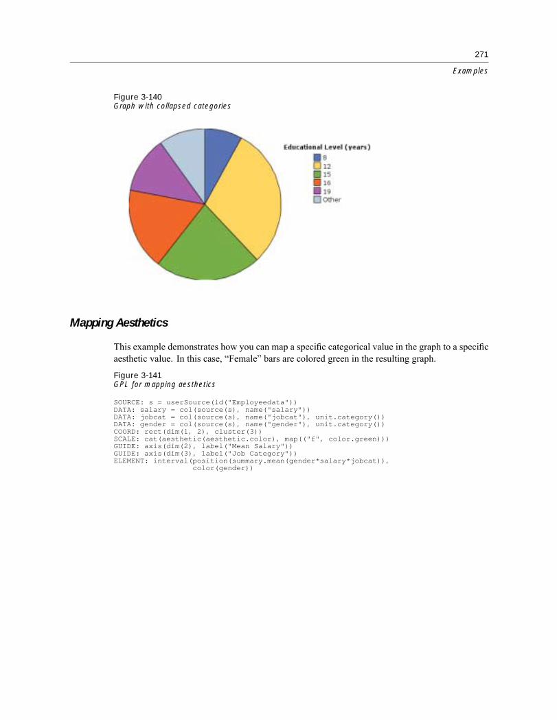
271

Examples

Figure 3-140Graph with collapsed categories

Mapping Aesthetics

This example demonstrates how you can map a speciÞc categorical value in the graph to a speciÞcaesthetic value. In this case, �Female� bars are colored green in the resulting graph.

Figure 3-141GPL for mapping aesthetics

SOURCE: s = userSource(id("Employeedata"))DATA: salary = col(source(s), name("salary"))DATA: jobcat = col(source(s), name("jobcat"), unit.category())DATA: gender = col(source(s), name("gender"), unit.category())COORD: rect(dim(1, 2), cluster(3))SCALE: cat(aesthetic(aesthetic.color), map(("f", color.green)))GUIDE: axis(dim(2), label("Mean Salary"))GUIDE: axis(dim(3), label("Job Category"))ELEMENT: interval(position(summary.mean(gender*salary*jobcat)),

color(gender))

272

Chapter 3

Figure 3-142Graph with mapped aesthetics

Faceting by Separate Variables

This example demonstrates how you can create facets based on separate variables, so that eachfacet shows the different variable information. Note that you can do something similar withnesting. For more information, see Line Chart with Separate Scales on p. 257.

Figure 3-143GPL for faceting by separate variables

SOURCE: s = userSource(id("Employeedata"))DATA: jobcat = col(source(s), name("jobcat"), unit.category())DATA: salary = col(source(s), name("salary"))DATA: salbegin = col(source(s), name("salbegin"))ELEMENT: schema(position(bin.quantile.letter(jobcat*salbegin*"Beginning Salary"+

jobcat*salary*"Current Salary")))

273

Examples

Figure 3-144Faceting by separate variables

Grouping by Separate Variables

This example demonstrates how you can create groups based on separate variables, so that eachinstance of the graphic element shows the different variable information. In this example, you arecomparing the results of two variables across a categorical variable.

Figure 3-145GPL for grouping by separate variables

SOURCE: s = userSource(id("Employeedata"))DATA: salbegin=col(source(s), name("salbegin"))DATA: salary=col(source(s), name("salary"))DATA: educ=col(source(s), name("educ"), unit.category())GUIDE: axis(dim(1), label("Educational Level (years)"))ELEMENT: line(position(summary.mean(educ*salary)),color("Current Salary"))ELEMENT: line(position(summary.mean(educ*salbegin)),color("Beginning Salary"))

274

Chapter 3

Figure 3-146Grouping by separate variables

Clustering Separate Variables

This example demonstrates how you can cluster separate variables.

Figure 3-147GPL for clustering separate variables

SOURCE: s = userSource(id("Employeedata"))DATA: jobcat = col(source(s), name("jobcat"), unit.category())DATA: salary = col(source(s), name("salary"))DATA: salbegin = col(source(s), name("salbegin"))COORD: rect(cluster(3))SCALE: linear(dim(2), include(0.0))GUIDE: axis(dim(2), label("Mean"))GUIDE: axis(dim(3), label("Job Category"))ELEMENT: interval(position(summary.mean("Beginning Salary"*salbegin*jobcat)),

color("Beginning Salary"))ELEMENT: interval(position(summary.mean("Current Salary"*salary*jobcat)),

color("Current Salary"))

275

Examples

Figure 3-148Clustering separate variables

Binning over Categorical Values

This example demonstrates how you use binning to show the distribution of a continuous variableover categorical values.

Figure 3-149GPL for binning over categorical values

SOURCE: s = userSource(id("Employeedata"))DATA: jobcat = col(source(s), name("jobcat"), unit.category())DATA: salary = col(source(s), name("salary"))GUIDE: axis(dim(1), label("Employment Category"))GUIDE: axis(dim(2), label("Current Salary"))GUIDE: legend(aesthetic(aesthetic.color), label("Count"))ELEMENT: polygon(position(bin.rect(jobcat*salary, dim(2))), color(summary.count()))

276

Chapter 3

Figure 3-150Binning over categorical values

Categorical Heat MapFigure 3-151GPL for categorical heat map

SOURCE: s = userSource(id("Employeedata"))DATA: gender = col(source(s), name("gender"), unit.category())DATA: educ = col(source(s), name("educ"), unit.category())DATA: salary = col(source(s), name("salary"))GUIDE: axis(dim(1), label("Educational Level"))GUIDE: axis(dim(2), label("Gender"))GUIDE: legend(aesthetic(aesthetic.color), label("Mean Salary"))ELEMENT: point(position(educ*gender), shape(shape.square), size(size."10%"),

color(summary.mean(salary)))

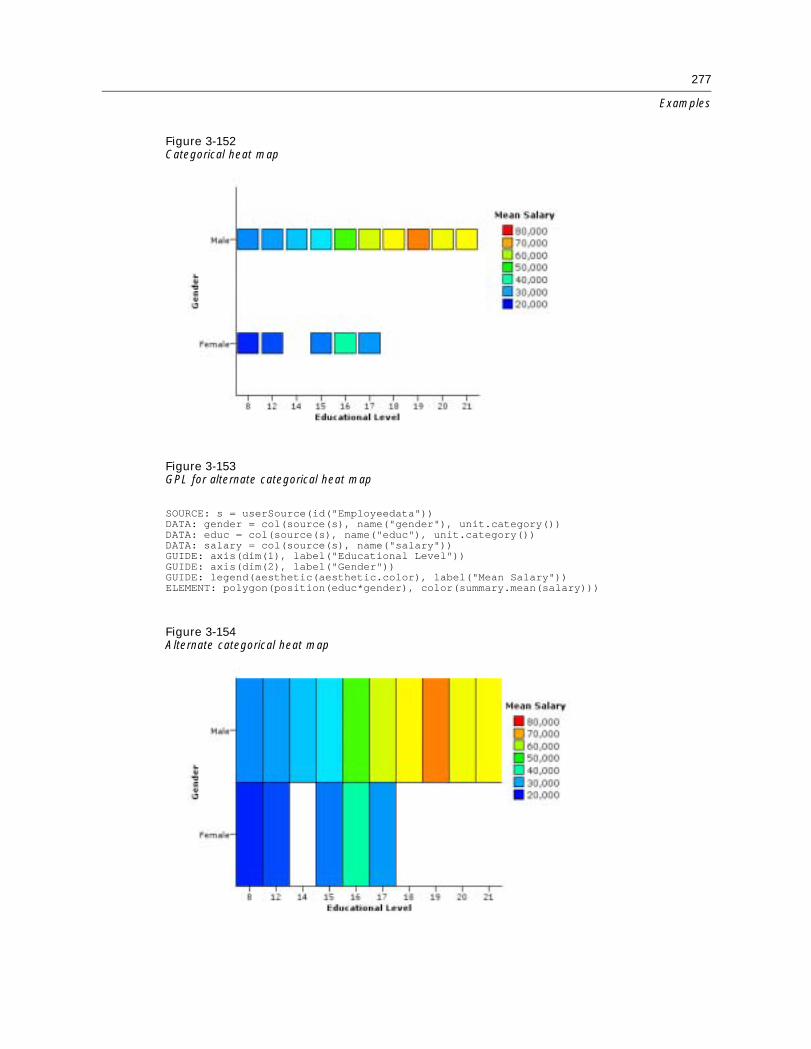
277

Examples

Figure 3-152Categorical heat map

Figure 3-153GPL for alternate categorical heat map

SOURCE: s = userSource(id("Employeedata"))DATA: gender = col(source(s), name("gender"), unit.category())DATA: educ = col(source(s), name("educ"), unit.category())DATA: salary = col(source(s), name("salary"))GUIDE: axis(dim(1), label("Educational Level"))GUIDE: axis(dim(2), label("Gender"))GUIDE: legend(aesthetic(aesthetic.color), label("Mean Salary"))ELEMENT: polygon(position(educ*gender), color(summary.mean(salary)))

Figure 3-154Alternate categorical heat map

278

Chapter 3

Creating Categories Using the eval Function

This example demonstrates how you can use the eval function to create categories based onan expression.

Figure 3-155GPL for creating categories with the eval function

SOURCE: s = userSource(id("Employeedata"))DATA: salbegin = col(source(s), name("salbegin"))DATA: salary = col(source(s), name("salary"))DATA: educ = col(source(s), name("educ"))TRANS: college = eval(educ>12 ? "College" : "No College")GUIDE: axis(dim(2), label("Current Salary"))GUIDE: axis(dim(1), label("Beginning Salary"))ELEMENT: point(position(salbegin*salary), color(college))

Figure 3-156Creating categories with the eval function

Appendix

AAAAGPL Constants

Color Constantsaliceblue aqua azure bisqueblack blanchedalmond blue bluevioletbrown burlywood cadetblue chartreusechocolate coral cornßowerblue cornsilkcrimson cyan darkblue darkcyandarkgoldenrod darkgray darkgreen darkgreydarkkhaki darkmagenta darkolivegreen darkorangedarkorchid darkred darksalmon darkseagreendarkslateblue darkslategray darkslategrey darkturquoisedarkviolet deeppink deepskyblue dimgraydimgrey dodgerblue Þrebrick ßoralwhiteforestgreen fuchsia gainsboro ghostwhitegold goldenrod gray greygreen greenyellow honeydew hotpinkindianred indigo ivory khakilavender lavenderblush lawngreen lemonchiffonlightblue lightcoral lightcyan lightgoldenrodyellowlightgray lightgreen lightgrey lightpinklightsalmon lightseagreen lightskyblue lightslategraylightslategrey lightsteelblue lightyellow limelimegreenlinen magenta maroon mediumaquamarinemediumblue mediumorchid mediumpurple mediumseagreenmediumslateblue mediumspringgreen mediumturquoise mediumvioletredmidnightblue mintcream mistyrose moccasinnavajowhite navy oldlace oliveolivedrab orange orangered orchidpalegoldenrod palegreen paleturquoise palevioletredpapayawhip peachpuff peru pinkplum powderblue purple redrosybrown royalblue saddlebrown salmon

279

280

Appendix A

sandybrown seagreen seashell siennasilver skyblue slateblue slategrayslategrey snow springgreen steelbluetan teal thistle tomato

turquoise violet wheat whitewhitesmoke yellow yellowgreen

Shape Constants

The following constants are all the valid constants for the different graphic element types. Notethat the constants for the edge graphic element appear in multiple tables.Table A-1Shape constants for interval elements

ibeam line square

Table A-2Shape constants for edge and point elementsarrow bowtie circle cross

female ßower ibeam linemale plus pentagon square

star

Table A-3Shape constants for edge, line, and path elements

dash dash_1_dot dash_2_dots dash_3_dotsdash_2x dash_3x dash_4_dots dash_dash2xhalf_dash solid

Size Constantstiny small medium largehuge

Pattern Constantscheckered grid grid2 grid3grid4 grid5 mesh mesh2mesh3 mesh4 mesh5 plusespluses2 solid

Bibliography

Wilkinson, L. 2005. The Grammar of Graphics, 2nd ed. New York: Springer-Verlag.

281

Index

aestheticMaximum function (GPL), 60aestheticMinimum function (GPL), 60aestheticMissing function (GPL), 61algebra (GPL), 4area element (GPL), 48asn scale (GPL), 32atanh scale (GPL), 33axis guide (GPL), 42

bar element (GPL), 48base function (GPL), 62base.aesthetic function (GPL), 62base.all function (GPL), 63base.coordinate function (GPL), 64begin function (GPL), 64�65beta function (GPL), 65bin.dot function (GPL), 66bin.hex function (GPL), 68bin.quantile.letter function (GPL), 70bin.rect function (GPL), 71binCount function (GPL), 73binStart function (GPL), 74binWidth function (GPL), 74boxplot (GPL), 54

cat (categorical) scale (GPL), 33chiSquare function (GPL), 75closed function (GPL), 76cluster function (GPL), 76col function (GPL), 78collapse function (GPL), 79collision modiÞers (GPL)difference, 54dodge, 55dodge.asymmetric, 55dodge.symmetric, 56jitter, 56stack, 57

color function (GPL), 80�81color.brightness function (GPL), 82color.hue function (GPL), 84color.saturation function (GPL), 85COMMENT statement (GPL), 23constants (GPL)color, 279pattern, 280shape, 280size, 280user, 6

COORD statement (GPL), 26

coordinate types (GPL)parallel, 27polar, 28polar.theta, 29project, 156rect (rectangular), 30

coordinates (GPL), 7csvSource function (GPL), 86

DATA statement (GPL), 25dataMaximum function (GPL), 87dataMinimum function (GPL), 87delta function (GPL), 87density.beta function (GPL), 88density.chiSquare function (GPL), 89density.exponential function (GPL), 90density.f function (GPL), 91density.gamma function (GPL), 92density.kernel function (GPL), 93density.logistic function (GPL), 95density.normal function (GPL), 96density.poisson function (GPL), 97density.studentizedRange function (GPL), 98density.t function (GPL), 99density.uniform function (GPL), 100density.weibull function (GPL), 101difference collision modiÞer (GPL), 54dim function (GPL), 102dodge collision modiÞer (GPL), 55dodge.asymmetric collision modiÞer (GPL), 55dodge.symmetric collision modiÞer (GPL), 56

edge element (GPL), 49ELEMENT statement (GPL), 47element types (GPL)area, 48bar, 48edge, 49interval, 49line, 50path, 51point, 52polygon, 53schema, 54

end function (GPL), 104eval function (GPL), 104exclude function (GPL), 108exponent function (GPL), 109exponential function (GPL), 109

282

283

Index

f function (GPL), 110footnote (GPL), 44�45format function (GPL), 110from function (GPL), 111functions (GPL)aestheticMaximum, 60aestheticMinimum, 60aestheticMissing, 61base, 62base.aesthetic, 62base.all, 63base.coordinate, 64begin, 64�65beta, 65bin.dot, 66bin.hex, 68bin.quantile.letter, 70bin.rect, 71binCount, 73binStart, 74binWidth, 74chiSquare, 75closed, 76cluster, 76col, 78collapse, 79color, 80�81color.brightness, 82color.hue, 84color.saturation, 85csvSource, 86dataMaximum, 87dataMinimum, 87delta, 87density.beta, 88density.chiSquare, 89density.exponential, 90density.f, 91density.gamma, 92density.kernel, 93density.logistic, 95density.normal, 96density.poisson, 97density.studentizedRange, 98density.t, 99density.uniform, 100density.weibull, 101dim, 102end, 104eval, 104exclude, 108exponent, 109exponential, 109f, 110format, 110from, 111gamma, 111

gap, 112gridlines, 112In, 112include, 113index, 114iter, 114jump, 115label, 115, 117layout.circle, 117layout.dag, 119layout.grid, 120layout.network, 121layout.random, 122layout.tree, 123link.alpha, 125link.complete, 126link.delaunay, 128link.distance, 129link.gabriel, 131link.hull, 132link.inßuence, 134link.join, 135link.mst, 137link.neighbor, 138link.relativeNeighborhood, 140link.sequence, 141link.tsp, 143logistic, 144map, 145mapSource, 146mapVariables, 146marron, 147max, 147min, 148mirror, 148missing.gap, 149missing.interpolate, 149missing.wings, 150noConstant, 150node, 150normal, 151notIn, 151opposite, 152origin, 152�153poisson, 154position, 154preserveStraightLines, 156proportion, 157reßect, 157region.conÞ.count, 158region.conÞ.mean, 159region.conÞ.percent.count, 161region.conÞ.smooth, 162region.spread.range, 163region.spread.sd, 165region.spread.se, 166reverse, 168

284

Index

root, 168scale, 169�171segments, 172shape, 172showAll, 173size, 173smooth.cubic, 175smooth.linear, 176smooth.loess, 178smooth.mean, 179smooth.median, 180smooth.quadratic, 183smooth.spline, 182smooth.step, 183sort.data, 185sort.natural, 185sort.statistic, 186sort.values, 187split, 187start, 188startAngle, 189studentizedRange, 189summary.count, 190summary.count.cumulative, 191summary.max, 193summary.mean, 195summary.min, 196summary.percent, 198summary.percent.count, 198summary.percent.count.cumulative, 200summary.percent.cumulative, 201summary.percent.sum, 202summary.percent.sum.cumulative, 203summary.sum, 205summary.sum.cumulative, 206t, 208texture.pattern, 208tick, 209to, 210transparency, 210transpose, 212uniform, 212unit.percent, 213userSource, 213values, 214weibull, 214weight, 215wrap, 215

gamma function (GPL), 111gap function (GPL), 112GPLalgebra, 4algebra and coordinate interaction, 7changes, 20clustering, 17color constants, 279

constants, color, 279constants, pattern, 280constants, shape, 280constants, size, 280data sources for examples, 217example data sources, 217faceting, 15introduction, 1operator precedence, 5operators, 4paneling, 15pattern constants, 280shape constants, 280size constants, 280stacking, 13syntax rules, 3unity variable, 6user constants, 6using aesthetics, 18

GRAPH statement (GPL), 24graphic element types (GPL)area, 48bar, 48edge, 49interval, 49line, 50path, 51point, 52polygon, 53schema, 54

graphic elements (GPL), 47gridlines function (GPL), 112GUIDE statement (GPL), 42guide types (GPL)axis, 42legend, 43text.footnote, 44text.subfootnote, 44text.subsubfootnote, 45text.subtitle, 45text.title, 46

In function (GPL), 112include function (GPL), 113index function (GPL), 114interval element (GPL), 49iter function (GPL), 114

jitter collision modiÞer (GPL), 56jump function (GPL), 115

label function (GPL), 115, 117layout.circle function (GPL), 117layout.dag function (GPL), 119layout.grid function (GPL), 120layout.network function (GPL), 121

285

Index

layout.random function (GPL), 122layout.tree function (GPL), 123legend guide (GPL), 43line element (GPL), 50linear scale (GPL), 34link.alpha function (GPL), 125link.complete function (GPL), 126link.delaunay function (GPL), 128link.distance function (GPL), 129link.gabriel function (GPL), 131link.hull function (GPL), 132link.inßuence function (GPL), 134link.join function (GPL), 135link.mst function (GPL), 137link.neighbor function (GPL), 138link.relativeNeighborhood function (GPL), 140link.sequence function (GPL), 141link.tsp function (GPL), 143log scale (GPL), 35logistic function (GPL), 144logit scale (GPL), 36

map function (GPL), 145mapSource function (GPL), 146mapVariables function (GPL), 146marron function (GPL), 147max function (GPL), 147min function (GPL), 148mirror function (GPL), 148missing.gap function (GPL), 149missing.interpolate function (GPL), 149missing.wings function (GPL), 150

noConstant function (GPL), 150node function (GPL), 150normal function (GPL), 151notIn function (GPL), 151

operator precedence (GPL), 5operators (GPL), 4opposite function (GPL), 152origin function (GPL), 152�153

PAGE statement (GPL), 23parallel coordinates (GPL), 27path element (GPL), 51point element (GPL), 52poisson function (GPL), 154polar coordinates (GPL), 28polar.theta coordinates (GPL), 29polygon element (GPL), 53position function (GPL), 154pow scale (GPL), 37preserveStraightLines function (GPL), 156prob scale (GPL), 37probit scale (GPL), 38

project coordinates (GPL), 156proportion function (GPL), 157

rect (rectangular) coordinates (GPL), 30reßect function (GPL), 157region.conÞ.count function (GPL), 158region.conÞ.mean function (GPL), 159region.conÞ.percent.count function (GPL), 161region.conÞ.smooth function (GPL), 162region.spread.range function (GPL), 163region.spread.sd function (GPL), 165region.spread.se function (GPL), 166reverse function (GPL), 168root function (GPL), 168

safeLog scale (GPL), 39safePower scale (GPL), 40scale function (GPL), 169�171SCALE statement (GPL), 31scale types (GPL), 32asn, 32atanh, 33cat (categorical), 33linear, 34log, 35logit, 36pow, 37prob, 37probit, 38safeLog, 39safePower, 40time, 41

schema element (GPL), 54segments function (GPL), 172shape function (GPL), 172showAll function (GPL), 173size function (GPL), 173smooth.cubic function (GPL), 175smooth.linear function (GPL), 176smooth.loess function (GPL), 178smooth.mean function (GPL), 179smooth.median function (GPL), 180smooth.quadratic function (GPL), 183smooth.spline function (GPL), 182smooth.step function (GPL), 183sort.data function (GPL), 185sort.natural function (GPL), 185sort.statistic function (GPL), 186sort.values function (GPL), 187SOURCE statement (GPL), 25split function (GPL), 187stack collision modiÞer (GPL), 57start function (GPL), 188startAngle function (GPL), 189statements (GPL), 22COMMENT, 23

286

Index

COORD, 26DATA, 25ELEMENT, 47GRAPH, 24GUIDE, 42PAGE, 23SCALE, 31SOURCE, 25TRANS, 26

studentizedRange function (GPL), 189subfootnote guide (GPL), 44subsubfootnote guide (GPL), 45subtitle guide (GPL), 45summary.count function (GPL), 190summary.count.cumulative function (GPL), 191summary.max function (GPL), 193summary.mean function (GPL), 195summary.min function (GPL), 196summary.percent function (GPL), 198summary.percent.count function (GPL), 198summary.percent.count.cumulative function (GPL), 200summary.percent.cumulative function (GPL), 201summary.percent.sum function (GPL), 202summary.percent.sum.cumulative function (GPL), 203summary.sum function (GPL), 205�206syntax rulesGPL, 3

t function (GPL), 208text.footnote guide (GPL), 44text.subfootnote guide (GPL), 44text.subsubfootnote guide (GPL), 45text.subtitle guide (GPL), 45text.title guide (GPL), 46texture.pattern function (GPL), 208ticks function (GPL), 209time scale (GPL), 41title 2 (GPL), 45title guide (GPL), 46to function (GPL), 210TRANS statement (GPL), 26transparency function (GPL), 210transpose function (GPL), 212

uniform function (GPL), 212unit.percent function (GPL), 213unity variable (GPL), 6user constants (GPL), 6userSource function (GPL), 213

values function (GPL), 214

weibull function (GPL), 214weight function (GPL), 215

wrap function (GPL), 215

SPSS 15.0 GPL Reference Guide - Kuwait University Reference Guide.pdf · SPSS 15.0 GPL Reference...

Documents

Transcript of SPSS 15.0 GPL Reference Guide - Kuwait University Reference Guide.pdf · SPSS 15.0 GPL Reference...