Springer Optimization and Its Applications

VOLUME 106

Managing EditorPanos M. Pardalos (University of Florida)

Editor–Combinatorial OptimizationDing-Zhu Du (University of Texas at Dallas)

Advisory BoardJ. Birge (University of Chicago)C.A. Floudas (Princeton University)F. Giannessi (University of Pisa)H.D. Sherali (Virginia Polytechnic and State University)T. Terlaky (McMaster University)Y. Ye (Stanford University)

Aims and ScopeOptimization has been expanding in all directions at an astonishing rateduring the last few decades. New algorithmic and theoretical techniqueshave been developed, the diffusion into other disciplines has proceeded at arapid pace, and our knowledge of all aspects of the field has grown even moreprofound. At the same time, one of the most striking trends in optimizationis the constantly increasing emphasis on the interdisciplinary nature of thefield. Optimization has been a basic tool in all areas of applied mathematics,engineering, medicine, economics, and other sciences.The series Springer Optimization and Its Applications publishes undergrad-uate and graduate textbooks, monographs and state-of-the-art expositorywork that focus on algorithms for solving optimization problems and alsostudy applications involving such problems. Some of the topics coveredinclude nonlinear optimization (convex and nonconvex), network flowproblems, stochastic optimization, optimal control, discrete optimization,multi-objective programming, description of software packages, approxima-tion techniques and heuristic approaches.

More information about this series at http://www.springer.com/series/7393

Antonio José Vázquez ÁlvarezRichard Scott Erwin

An Introduction to OptimalSatellite Range Scheduling

123

Antonio José Vázquez ÁlvarezNational Research CouncilAlbuquerque, NM, USA

Richard Scott ErwinAir Force Research LaboratorySpace Vehicles Directorate, KirtlandAlbuquerque, NM, USA

ISSN 1931-6828 ISSN 1931-6836 (electronic)Springer Optimization and Its ApplicationsISBN 978-3-319-25407-4 ISBN 978-3-319-25409-8 (eBook)DOI 10.1007/978-3-319-25409-8

Library of Congress Control Number: 2015953220

Mathematics Subject Classification (2010): 68M20, 90B35, 90B36, 90-02, 68Q25, 90C39, 97K30,05C85, 91A40, 91A80, 91A10, 91A18, 62C10

Springer Cham Heidelberg New York Dordrecht London© Springer International Publishing Switzerland 2015This work is subject to copyright. All rights are reserved by the Publisher, whether the whole or part ofthe material is concerned, specifically the rights of translation, reprinting, reuse of illustrations, recitation,broadcasting, reproduction on microfilms or in any other physical way, and transmission or informationstorage and retrieval, electronic adaptation, computer software, or by similar or dissimilar methodologynow known or hereafter developed.The use of general descriptive names, registered names, trademarks, service marks, etc. in this publicationdoes not imply, even in the absence of a specific statement, that such names are exempt from the relevantprotective laws and regulations and therefore free for general use.The publisher, the authors and the editors are safe to assume that the advice and information in this bookare believed to be true and accurate at the date of publication. Neither the publisher nor the authors orthe editors give a warranty, express or implied, with respect to the material contained herein or for anyerrors or omissions that may have been made.

Printed on acid-free paper

Springer International Publishing AG Switzerland is part of Springer Science+Business Media (www.springer.com)

To my parents. A. J.

To my wife, my son, and my parents. R. S.

Preface

The problem of scheduling interactions among satellites and ground stations hasbeen around for decades, and most of the literature tackling this problem has focusedon approximate solutions. In this book we have tried to find the optimal solution tothis problem and some of its variants and also to unify criteria and notation acrossthe satellite range scheduling literature. To our knowledge, this is the first work thatwill accomplish both objectives.

We wrote this book as a result of a 2-year (2013–2015) postdoctoral fellowshipat the Air Force Research Laboratory, funded by the National Research Council.The major results contained herein were published as a series of conference andjournal papers during this period. This work, although based on these publications,considerably extends them by solving new problems and binding them together asa whole.

This endeavor has not been easy, with telecommunication and control engineer-ing backgrounds for tackling a problem from operations research. We think howeverthat this combination provides increased value to this book, and we have in fact triedto make it accessible to those readers that are facing this problem for the first time.This book is also aimed at satellite operations engineers and scheduling algorithmdesigners, as we here provide reference (optimal) solutions to this problem and someof its most important variants.

We are conscious that we are only scratching the surface on satellite rangescheduling, but we have tried to provide a strong framework over which keep findingsolutions to more complex problems in this field. We hope this book keeps up withthe high standards of previous literature in this field, and more importantly, we hopethis book to be useful to students and algorithm designers.

Albuquerque, NM, USA Antonio José Vázquez ÁlvarezKirtland AFB, NM, USA Richard Scott ErwinApril 2015

vii

Acknowledgments

I would like to thank my parents, Anun and Javier, for all their encouragement, notonly during this period but throughout all my life. This work would not be possiblewithout them, which always have been and will be my example. I want to thank mybrother Luis too for his encouragement and support in the distance. Very especiallyI would like to thank my fiancée Nelmy Jerez, meeting her has truly changed mylife, and her encouragement and love motivated me to continue with this endeavor.

I would like to thank my research advisor R. Scott Erwin, coauthor of this book,for all his help and trust during this period. He has always pointed the research inthe right direction if I diverged too much, and since the beginning he has alwaysshared his knowledge and gave me several pieces of valuable advice. I would alsolike to thank all the people I have met in AFRL, COSMIAC, and UNM, especiallyAlonzo Vera, Carolin Früh, Craig Kief, David Alexander, Frederick Leve, MoribaJah, Robert Terselic, and many others who have been very helpful and friendly.

I am very grateful to the National Research Council1 for this opportunity andfor all their support during this period, especially to Peggy Wilson, who has alwaysanswered my never-ending lists of questions.

I would like to thank Springer for their trust in this project since its inception andfor providing the LATEX monograph template. Finally I would like to thank Springer,Scitepress, and IEEE for granting us permission for recasting some materials fromour previous work. We have generated all the diagrams with DIA and Inkscape andthe simulation maps and graphs with MATLAB and did the typesetting in MiKTeX.

A. J.

I would like to thank first my wife, Kim, and my son, Ian; it is the time I have spentaway from them, or the times I have been home but not present, that are the realprice paid for accomplishments such as this.

1This research was performed while the author held a National Research Council ResearchAssociateship Award at the Air Force Research Laboratory (AFRL).

ix

x Acknowledgments

I would like to thank my parents, Richard and Barbara, for giving me theopportunities in life that led to the successes I have enjoyed.

Finally, I’d like to thank my coauthor, Antonio, for his incredible effortsproducing the results herein as well as in preparing this monograph.

R. S.

Contents

Part I Introduction

1 Motivation . . . . . . . . . . . . . . . . . . . . . . . . . . . . . . . . . . . . . . . . . . . . . . . . . . . . . . . . . . . . . . . . . . . . 31.1 Motivation . . . . . . . . . . . . . . . . . . . . . . . . . . . . . . . . . . . . . . . . . . . . . . . . . . . . . . . . . . . . . . . 31.2 Why Optimal Scheduling?. . . . . . . . . . . . . . . . . . . . . . . . . . . . . . . . . . . . . . . . . . . . . . 41.3 Why this Book? . . . . . . . . . . . . . . . . . . . . . . . . . . . . . . . . . . . . . . . . . . . . . . . . . . . . . . . . . 41.4 Structure of the Book . . . . . . . . . . . . . . . . . . . . . . . . . . . . . . . . . . . . . . . . . . . . . . . . . . . 51.5 Main Contributions . . . . . . . . . . . . . . . . . . . . . . . . . . . . . . . . . . . . . . . . . . . . . . . . . . . . . 7References . . . . . . . . . . . . . . . . . . . . . . . . . . . . . . . . . . . . . . . . . . . . . . . . . . . . . . . . . . . . . . . . . . . . . 9

2 Scheduling Process . . . . . . . . . . . . . . . . . . . . . . . . . . . . . . . . . . . . . . . . . . . . . . . . . . . . . . . . . . . 112.1 Scheduling Process. . . . . . . . . . . . . . . . . . . . . . . . . . . . . . . . . . . . . . . . . . . . . . . . . . . . . . 112.2 Scheduler Characteristics . . . . . . . . . . . . . . . . . . . . . . . . . . . . . . . . . . . . . . . . . . . . . . . 152.3 Satellite Range Scheduling Problems . . . . . . . . . . . . . . . . . . . . . . . . . . . . . . . . . . 152.4 Issues Beyond the Scope of this Text . . . . . . . . . . . . . . . . . . . . . . . . . . . . . . . . . . 16References . . . . . . . . . . . . . . . . . . . . . . . . . . . . . . . . . . . . . . . . . . . . . . . . . . . . . . . . . . . . . . . . . . . . . 17

Part II Satellite Range Scheduling

3 The Satellite Range Scheduling Problem . . . . . . . . . . . . . . . . . . . . . . . . . . . . . . . . . . 213.1 Problem Formulation . . . . . . . . . . . . . . . . . . . . . . . . . . . . . . . . . . . . . . . . . . . . . . . . . . . 21

3.1.1 Model for the Scenario . . . . . . . . . . . . . . . . . . . . . . . . . . . . . . . . . . . . . . . . . 223.1.2 Model for the Requests . . . . . . . . . . . . . . . . . . . . . . . . . . . . . . . . . . . . . . . . . 233.1.3 Problem Constraints . . . . . . . . . . . . . . . . . . . . . . . . . . . . . . . . . . . . . . . . . . . . 253.1.4 Schedule Metrics. . . . . . . . . . . . . . . . . . . . . . . . . . . . . . . . . . . . . . . . . . . . . . . . 32

3.2 Complexity of SRS . . . . . . . . . . . . . . . . . . . . . . . . . . . . . . . . . . . . . . . . . . . . . . . . . . . . . 343.2.1 Introduction to Complexity Theory . . . . . . . . . . . . . . . . . . . . . . . . . . . . 343.2.2 Complexity of the SRS Problem . . . . . . . . . . . . . . . . . . . . . . . . . . . . . . . 34

xi

xii Contents

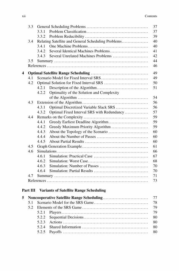
3.3 General Scheduling Problems . . . . . . . . . . . . . . . . . . . . . . . . . . . . . . . . . . . . . . . . . . 373.3.1 Problem Classification . . . . . . . . . . . . . . . . . . . . . . . . . . . . . . . . . . . . . . . . . . 373.3.2 Problem Reducibility . . . . . . . . . . . . . . . . . . . . . . . . . . . . . . . . . . . . . . . . . . . 39

3.4 Relating Satellite and General Scheduling Problems. . . . . . . . . . . . . . . . . . 403.4.1 One Machine Problems . . . . . . . . . . . . . . . . . . . . . . . . . . . . . . . . . . . . . . . . . 403.4.2 Several Identical Machines Problems. . . . . . . . . . . . . . . . . . . . . . . . . . 413.4.3 Several Unrelated Machines Problems . . . . . . . . . . . . . . . . . . . . . . . . 42

3.5 Summary . . . . . . . . . . . . . . . . . . . . . . . . . . . . . . . . . . . . . . . . . . . . . . . . . . . . . . . . . . . . . . . . 44References . . . . . . . . . . . . . . . . . . . . . . . . . . . . . . . . . . . . . . . . . . . . . . . . . . . . . . . . . . . . . . . . . . . . . 46

4 Optimal Satellite Range Scheduling . . . . . . . . . . . . . . . . . . . . . . . . . . . . . . . . . . . . . . . 494.1 Scenario Model for Fixed Interval SRS . . . . . . . . . . . . . . . . . . . . . . . . . . . . . . . . 494.2 Optimal Solution for Fixed Interval SRS . . . . . . . . . . . . . . . . . . . . . . . . . . . . . . 50

4.2.1 Description of the Algorithm. . . . . . . . . . . . . . . . . . . . . . . . . . . . . . . . . . . 514.2.2 Optimality of the Solution and Complexity

of the Algorithm . . . . . . . . . . . . . . . . . . . . . . . . . . . . . . . . . . . . . . . . . . . . . . . . 544.3 Extension of the Algorithm . . . . . . . . . . . . . . . . . . . . . . . . . . . . . . . . . . . . . . . . . . . . . 56

4.3.1 Optimal Discretized Variable Slack SRS . . . . . . . . . . . . . . . . . . . . . . 564.3.2 Optimal Fixed Interval SRS with Redundancy . . . . . . . . . . . . . . . . 57

4.4 Remarks on the Complexity . . . . . . . . . . . . . . . . . . . . . . . . . . . . . . . . . . . . . . . . . . . . 594.4.1 Greedy Earliest Deadline Algorithm. . . . . . . . . . . . . . . . . . . . . . . . . . . 594.4.2 Greedy Maximum Priority Algorithm . . . . . . . . . . . . . . . . . . . . . . . . . 594.4.3 About the Topology of the Scenario . . . . . . . . . . . . . . . . . . . . . . . . . . . 604.4.4 About the Number of Passes . . . . . . . . . . . . . . . . . . . . . . . . . . . . . . . . . . . 604.4.5 About Partial Results . . . . . . . . . . . . . . . . . . . . . . . . . . . . . . . . . . . . . . . . . . . 60

4.5 Graph Generation Example . . . . . . . . . . . . . . . . . . . . . . . . . . . . . . . . . . . . . . . . . . . . . 614.6 Simulations . . . . . . . . . . . . . . . . . . . . . . . . . . . . . . . . . . . . . . . . . . . . . . . . . . . . . . . . . . . . . . 66

4.6.1 Simulation: Practical Case . . . . . . . . . . . . . . . . . . . . . . . . . . . . . . . . . . . . . 674.6.2 Simulation: Worst Case. . . . . . . . . . . . . . . . . . . . . . . . . . . . . . . . . . . . . . . . . 684.6.3 Simulation: Number of Passes . . . . . . . . . . . . . . . . . . . . . . . . . . . . . . . . . 704.6.4 Simulation: Partial Results . . . . . . . . . . . . . . . . . . . . . . . . . . . . . . . . . . . . . 70

4.7 Summary . . . . . . . . . . . . . . . . . . . . . . . . . . . . . . . . . . . . . . . . . . . . . . . . . . . . . . . . . . . . . . . . 71References . . . . . . . . . . . . . . . . . . . . . . . . . . . . . . . . . . . . . . . . . . . . . . . . . . . . . . . . . . . . . . . . . . . . . 73

Part III Variants of Satellite Range Scheduling

5 Noncooperative Satellite Range Scheduling. . . . . . . . . . . . . . . . . . . . . . . . . . . . . . . 775.1 Scenario Model for the SRS Game. . . . . . . . . . . . . . . . . . . . . . . . . . . . . . . . . . . . . 785.2 Elements of the SRS Game . . . . . . . . . . . . . . . . . . . . . . . . . . . . . . . . . . . . . . . . . . . . . 79

5.2.1 Players . . . . . . . . . . . . . . . . . . . . . . . . . . . . . . . . . . . . . . . . . . . . . . . . . . . . . . . . . . . 795.2.2 Sequential Decisions. . . . . . . . . . . . . . . . . . . . . . . . . . . . . . . . . . . . . . . . . . . . 805.2.3 Actions . . . . . . . . . . . . . . . . . . . . . . . . . . . . . . . . . . . . . . . . . . . . . . . . . . . . . . . . . . 805.2.4 Shared Information . . . . . . . . . . . . . . . . . . . . . . . . . . . . . . . . . . . . . . . . . . . . . 805.2.5 Payoffs . . . . . . . . . . . . . . . . . . . . . . . . . . . . . . . . . . . . . . . . . . . . . . . . . . . . . . . . . . 80

Contents xiii

5.2.6 Rationality . . . . . . . . . . . . . . . . . . . . . . . . . . . . . . . . . . . . . . . . . . . . . . . . . . . . . . 815.2.7 Extensive Form . . . . . . . . . . . . . . . . . . . . . . . . . . . . . . . . . . . . . . . . . . . . . . . . . 81

5.3 SRS Game with Perfect Information . . . . . . . . . . . . . . . . . . . . . . . . . . . . . . . . . . . 825.3.1 Description of the Algorithm. . . . . . . . . . . . . . . . . . . . . . . . . . . . . . . . . . . 835.3.2 Stackelberg Equilibrium Solution . . . . . . . . . . . . . . . . . . . . . . . . . . . . . . 875.3.3 Computational Complexity. . . . . . . . . . . . . . . . . . . . . . . . . . . . . . . . . . . . . 89

5.4 Limited Information Versions of the Problem . . . . . . . . . . . . . . . . . . . . . . . . . 895.4.1 SRS Game with Uncertain Priorities. . . . . . . . . . . . . . . . . . . . . . . . . . . 905.4.2 SRS Game with Uncertain Passes . . . . . . . . . . . . . . . . . . . . . . . . . . . . . 92

5.5 Remarks on the SRS Game . . . . . . . . . . . . . . . . . . . . . . . . . . . . . . . . . . . . . . . . . . . . . 935.5.1 Equilibrium vs. Security Strategy . . . . . . . . . . . . . . . . . . . . . . . . . . . . . . 935.5.2 Stackelberg Equilibrium vs. Nash Equilibrium . . . . . . . . . . . . . . . 935.5.3 Social Welfare and Price of Anarchy . . . . . . . . . . . . . . . . . . . . . . . . . . 945.5.4 Machine Scheduling vs. SRS . . . . . . . . . . . . . . . . . . . . . . . . . . . . . . . . . . 94

5.6 Graph Generation Example . . . . . . . . . . . . . . . . . . . . . . . . . . . . . . . . . . . . . . . . . . . . . 945.7 Simulations . . . . . . . . . . . . . . . . . . . . . . . . . . . . . . . . . . . . . . . . . . . . . . . . . . . . . . . . . . . . . . 1015.8 Summary . . . . . . . . . . . . . . . . . . . . . . . . . . . . . . . . . . . . . . . . . . . . . . . . . . . . . . . . . . . . . . . . 104References . . . . . . . . . . . . . . . . . . . . . . . . . . . . . . . . . . . . . . . . . . . . . . . . . . . . . . . . . . . . . . . . . . . . . 105

6 Robust Satellite Range Scheduling . . . . . . . . . . . . . . . . . . . . . . . . . . . . . . . . . . . . . . . . . 1076.1 Scenario Model for Robust SRS . . . . . . . . . . . . . . . . . . . . . . . . . . . . . . . . . . . . . . . 108

6.1.1 Complexity of the Robust SRS Problem. . . . . . . . . . . . . . . . . . . . . . . 1106.2 Restricted Robust SRS Problem . . . . . . . . . . . . . . . . . . . . . . . . . . . . . . . . . . . . . . . . 1106.3 Remarks regarding Multiple Scheduling Entities . . . . . . . . . . . . . . . . . . . . . 1146.4 Variants of the Robust SRS Problem . . . . . . . . . . . . . . . . . . . . . . . . . . . . . . . . . . . 116

6.4.1 Robust SRS with Random Priorities . . . . . . . . . . . . . . . . . . . . . . . . . . . 1166.4.2 Robust SRS with Random Durations . . . . . . . . . . . . . . . . . . . . . . . . . . 119

6.5 Considerations on the Basic SRS Problem . . . . . . . . . . . . . . . . . . . . . . . . . . . . 1236.6 Schedule Computation Example . . . . . . . . . . . . . . . . . . . . . . . . . . . . . . . . . . . . . . . 1246.7 Simulations . . . . . . . . . . . . . . . . . . . . . . . . . . . . . . . . . . . . . . . . . . . . . . . . . . . . . . . . . . . . . . 1246.8 Summary . . . . . . . . . . . . . . . . . . . . . . . . . . . . . . . . . . . . . . . . . . . . . . . . . . . . . . . . . . . . . . . . 126References . . . . . . . . . . . . . . . . . . . . . . . . . . . . . . . . . . . . . . . . . . . . . . . . . . . . . . . . . . . . . . . . . . . . . 128

7 Reactive Satellite Range Scheduling . . . . . . . . . . . . . . . . . . . . . . . . . . . . . . . . . . . . . . . 1297.1 Scenario Model for Reactive SRS . . . . . . . . . . . . . . . . . . . . . . . . . . . . . . . . . . . . . . 129

7.1.1 Complexity of the Reactive SRS Problem . . . . . . . . . . . . . . . . . . . . . 1317.2 Restricted Reactive SRS: Single Pass Update Model . . . . . . . . . . . . . . . . . 132

7.2.1 Overview of the Algorithm. . . . . . . . . . . . . . . . . . . . . . . . . . . . . . . . . . . . . 1327.2.2 Preprocessing . . . . . . . . . . . . . . . . . . . . . . . . . . . . . . . . . . . . . . . . . . . . . . . . . . . 1337.2.3 Recomputation . . . . . . . . . . . . . . . . . . . . . . . . . . . . . . . . . . . . . . . . . . . . . . . . . . 139

7.3 Restricted Reactive SRS: Multiple Pass Update Model . . . . . . . . . . . . . . . 1407.4 Schedule Computation Example . . . . . . . . . . . . . . . . . . . . . . . . . . . . . . . . . . . . . . . 1407.5 Summary . . . . . . . . . . . . . . . . . . . . . . . . . . . . . . . . . . . . . . . . . . . . . . . . . . . . . . . . . . . . . . . . 145References . . . . . . . . . . . . . . . . . . . . . . . . . . . . . . . . . . . . . . . . . . . . . . . . . . . . . . . . . . . . . . . . . . . . . 147

xiv Contents

8 Summary . . . . . . . . . . . . . . . . . . . . . . . . . . . . . . . . . . . . . . . . . . . . . . . . . . . . . . . . . . . . . . . . . . . . . . 1498.1 Conclusions . . . . . . . . . . . . . . . . . . . . . . . . . . . . . . . . . . . . . . . . . . . . . . . . . . . . . . . . . . . . . 1498.2 Future Work . . . . . . . . . . . . . . . . . . . . . . . . . . . . . . . . . . . . . . . . . . . . . . . . . . . . . . . . . . . . . 149

Glossary . . . . . . . . . . . . . . . . . . . . . . . . . . . . . . . . . . . . . . . . . . . . . . . . . . . . . . . . . . . . . . . . . . . . . . . . . . . 153

Index . . . . . . . . . . . . . . . . . . . . . . . . . . . . . . . . . . . . . . . . . . . . . . . . . . . . . . . . . . . . . . . . . . . . . . . . . . . . . . . 159

Acronyms

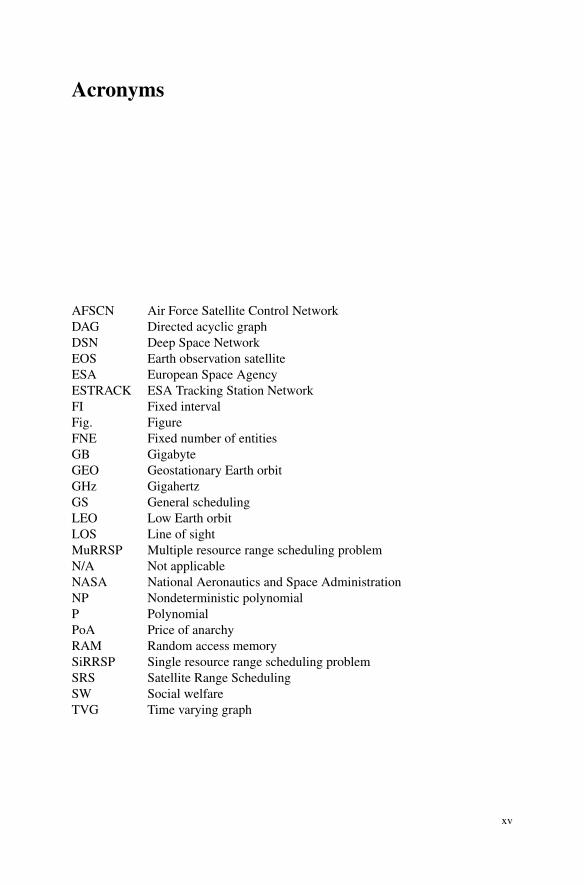
AFSCN Air Force Satellite Control NetworkDAG Directed acyclic graphDSN Deep Space NetworkEOS Earth observation satelliteESA European Space AgencyESTRACK ESA Tracking Station NetworkFI Fixed intervalFig. FigureFNE Fixed number of entitiesGB GigabyteGEO Geostationary Earth orbitGHz GigahertzGS General schedulingLEO Low Earth orbitLOS Line of sightMuRRSP Multiple resource range scheduling problemN/A Not applicableNASA National Aeronautics and Space AdministrationNP Nondeterministic polynomialP PolynomialPoA Price of anarchyRAM Random access memorySiRRSP Single resource range scheduling problemSRS Satellite Range SchedulingSW Social welfareTVG Time varying graph

xv

Symbols

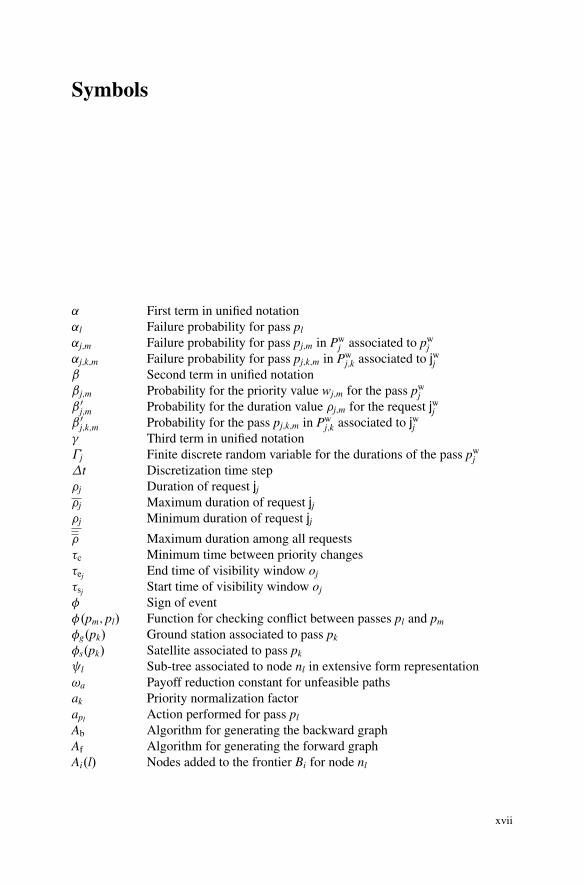
˛ First term in unified notation˛l Failure probability for pass pl

˛j;m Failure probability for pass pj;m in Pwj associated to pw

j˛j;k;m Failure probability for pass pj;k;m in Pw

j;k associated to jwjˇ Second term in unified notationˇj;m Probability for the priority value wj;m for the pass pw

jˇ0

j;m Probability for the duration value �j;m for the request jwjˇ0

j;k;m Probability for the pass pj;k;m in Pwj;k associated to jwj

� Third term in unified notation�j Finite discrete random variable for the durations of the pass pw

j�t Discretization time step�j Duration of request jj�j Maximum duration of request jj�j Minimum duration of request jj� Maximum duration among all requests�c Minimum time between priority changes�ej End time of visibility window oj

�sj Start time of visibility window oj

� Sign of event�.pm; pl/ Function for checking conflict between passes pl and pm

�g.pk/ Ground station associated to pass pk

�s.pk/ Satellite associated to pass pk

l Sub-tree associated to node nl in extensive form representation!a Payoff reduction constant for unfeasible pathsak Priority normalization factorapl Action performed for pass pl

Ab Algorithm for generating the backward graphAf Algorithm for generating the forward graphAi.l/ Nodes added to the frontier Bi for node nl

xvii

xviii Symbols

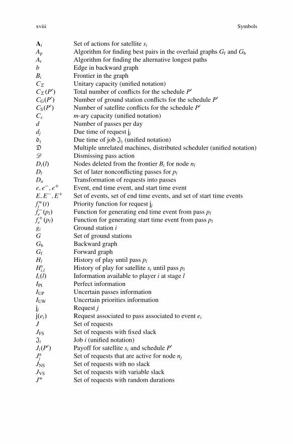
Ai Set of actions for satellite si

Ap Algorithm for finding best pairs in the overlaid graphs Gf and Gb

Ar Algorithm for finding the alternative longest pathsb Edge in backward graphBi Frontier in the graphC˙ Unitary capacity (unified notation)C˙.P0/ Total number of conflicts for the schedule P0CG.P0/ Number of ground station conflicts for the schedule P0CS.P0/ Number of satellite conflicts for the schedule P0Cx m-ary capacity (unified notation)d Number of passes per daydj Due time of request jjdj Due time of job Jj (unified notation)D Multiple unrelated machines, distributed scheduler (unified notation)D Dismissing pass actionDi.l/ Nodes deleted from the frontier Bi for node nl

Dl Set of later nonconflicting passes for pl

Dn Transformation of requests into passese; e�; eC Event, end time event, and start time eventE;E�;EC Set of events, set of end time events, and set of start time eventsf wj .t/ Priority function for request jj

f �e .pl/ Function for generating end time event from pass pl

f Ce .pl/ Function for generating start time event from pass pl

gi Ground station iG Set of ground stationsGb Backward graphGf Forward graphHl History of play until pass pl

Hsi;l History of play for satellite si until pass pl

Ii.l/ Information available to player i at stage lIPI Perfect informationIUP Uncertain passes informationIUW Uncertain priorities informationjj Request jj.ei/ Request associated to pass associated to event ei

J Set of requestsJFS Set of requests with fixed slackJi Job i (unified notation)Ji.P0/ Payoff for satellite si and schedule P0Ja

j Set of requests that are active for node nj

JNS Set of requests with no slackJVS Set of requests with variable slackJw Set of requests with random durations

Symbols xix

J.nj/ Set of requests associated to backtracking from nj to n0k1 Number of scheduling resourcesk2 Number of scheduling entitiesL Longest path in graph before the priority changeL0 Longest path in graph after the priority changeL.nj/ Longest path that includes node nj

Lb.ny; nz/ Longest path in Gb from node ny to nz

Lf.nx; ny/ Longest path in Gf from node nx to ny

mj Subpath in the graph associated to node nj

M Maximum number of possible priorities (durations) for passes withrandom priorities (durations)

Mc Maximum number of passes that change priority at the same timeMi Machine (unified notation)Mj Number of possible priorities (durations) for pass pw

j (request jwj )ndj Discrete due time of request jjnek Discrete end time of pass pk

ni Node in the graphnrj Discrete release time of request jjnsk Discrete start time of pass pk

n�.i; k/ Best node in Zi for current stage Zk with associated pass trackedn0.i; k/ Best node in Zi for current stage Zk with associated pass not trackedN Number of requests or passesoj Visibility window jO.�/ Big O notationpij Processing time of job Jj in machine Mi (unified notation)pvar

ij Variable processing time for job Jj in machine Mi (unified notation)pj Maximum processing time of job Jj (unified notation)pj Minimum processing time of job Jj (unified notation)pj;m Pass with associated failure probability ˛j;m generated from pw

jpw

j Pass with random prioritiespk Pass kp.ei/ Pass associated to event ei

P Multiple related machines (unified notation)P Initial set of passesP0;P00;Psub ScheduleQP Executed scheduleP� Optimal scheduleP�.t/ Updated optimal schedulePa

j Set of passes that are active for node nj

Pd Set of passes generated from the set of requests with random durationsPdR Robust schedule for the robust SRS problem with random durationsPf Feasible schedulePj

j Set of passes generated from request jj

xx Symbols

Pwj Set of passes with failure probabilities generated from pw

jPl Set of later passes for pl, including pl

PPl Precedence subset

Pnw Set of passes with uncertain prioritiesPR Robust schedule for the robust SRS problem with failure probabilitiesPs

i Subset of P in which passes are associated to si

Psmi Security schedule for si

Pw Initial set of passes with random prioritiesPwR Robust schedule for the robust SRS problem with random prioritiesP.nj/ Set of passes associated to backtracking from nj to n0P.t/ Set of passes with time-dependent priorities at time tP.t/jt2t1 Subset of P.t/, which passes have start times in the interval Œt1; t2�P

� � �Probability

q Maximum duration of all visibility windows in discretizationqj Duration of visibility window of discretized request jjqjk Maximum duration of pass pk associated to discretized request jjqjk Minimum duration of pass pk associated to discretized request jjrj Release time of request jjrj Release time of job Jj (unified notation)R Multiple unrelated machines (unified notation)Ri.k/ Best pair of nodes in Zi, computed from current stage Zk

sh Satellite hslead Leader satelliteS Set of satellites§ Sectiont Timet0 Initial timetek End time of pass pk

tsk Start time of pass pk

T Tracking pass actionT Duration of the scheduling horizonTg Reduced time for the game developmentUj Lateness of job Jj (unified notation)UŒ1; 10� Discrete uniform distribution with values between 1 and 10v Edge in (forward) graphwj Priority of job Jj (unified notation)wj;m Priority of pass pw

j;mwk Priority of pass pk

wkth.pz/ Threshold value for the priority of pass pz for current stage Zk

w.p. With probabilityWi.k/ Priorities associated to the best pair of nodes Ri.k/Wj Distribution of priorities for pw

j

Symbols xxi

ZC Stages associated to start time events in graphZ0 Initial stage in graphk � k˙w Metric of schedule, e.g., kP0k˙w

k � kE Expected metric of schedule, e.g., kP0kEh�its Set of passes sorted by start time, e.g., hP0its

O� Reduced information (unified notation), e.g., bwj; bUj

Q� Uncertainty (unified notation), e.g., epij; eUj

List of Figures

Fig. 1.1 Book structure . . . . . . . . . . . . . . . . . . . . . . . . . . . . . . . . . . . . . . . . . . . . . . . . . . . . . . . . 6

Fig. 2.1 Scheduling scenario . . . . . . . . . . . . . . . . . . . . . . . . . . . . . . . . . . . . . . . . . . . . . . . . . . 12Fig. 2.2 Scheduling process . . . . . . . . . . . . . . . . . . . . . . . . . . . . . . . . . . . . . . . . . . . . . . . . . . . 12Fig. 2.3 Visibility windows . . . . . . . . . . . . . . . . . . . . . . . . . . . . . . . . . . . . . . . . . . . . . . . . . . . . 13Fig. 2.4 Scheduling requests (based on visibility windows from Fig. 2.3) . . 14Fig. 2.5 Final schedule (based on requests from Fig. 2.4). . . . . . . . . . . . . . . . . . . . 14Fig. 2.6 Satellite Range Scheduling problems . . . . . . . . . . . . . . . . . . . . . . . . . . . . . . . . 16

Fig. 3.1 Time varying graph representing visibility betweenpairs ground station–satellite . . . . . . . . . . . . . . . . . . . . . . . . . . . . . . . . . . . . . . . . . 22

Fig. 3.2 Example of TVG modeling two visibility windowsfor two ground stations and two satellites: interactionbetween s1 and g2 only active at �s1 < t < �e1 (blue),and interaction between s2 and g1 only active at�s2 < t < �e2 (green) . . . . . . . . . . . . . . . . . . . . . . . . . . . . . . . . . . . . . . . . . . . . . . . . . . 23

Fig. 3.3 Request specification . . . . . . . . . . . . . . . . . . . . . . . . . . . . . . . . . . . . . . . . . . . . . . . . . 24Fig. 3.4 Types of requests: variable-slack (top), fixed-slack

(center), and no-slack (bottom) . . . . . . . . . . . . . . . . . . . . . . . . . . . . . . . . . . . . . . 26Fig. 3.5 Transformation of a request into a set of passes, with all

the possible combinations of start times and durationscomplying with the specification of the request, andtaking into account the duration of the discretization step . . . . . . . . . . 29

Fig. 3.6 Examples of conflicting passes. . . . . . . . . . . . . . . . . . . . . . . . . . . . . . . . . . . . . . . 31Fig. 3.7 Priorities of the passes generated from a request . . . . . . . . . . . . . . . . . . . . 33Fig. 3.8 Unified notation for representing scheduling problems . . . . . . . . . . . . . 38Fig. 3.9 SRS problems classification . . . . . . . . . . . . . . . . . . . . . . . . . . . . . . . . . . . . . . . . . . 46

Fig. 4.1 Centralized scheduler . . . . . . . . . . . . . . . . . . . . . . . . . . . . . . . . . . . . . . . . . . . . . . . . . 50Fig. 4.2 Relations between the algorithms for optimal SRS . . . . . . . . . . . . . . . . . 58Fig. 4.3 Set of passes . . . . . . . . . . . . . . . . . . . . . . . . . . . . . . . . . . . . . . . . . . . . . . . . . . . . . . . . . . 61Fig. 4.4 Event generation . . . . . . . . . . . . . . . . . . . . . . . . . . . . . . . . . . . . . . . . . . . . . . . . . . . . . . 62

xxiii

xxiv List of Figures

Fig. 4.5 Transition from stage Z0 to Z1. (a) Initial node. (b)Creation of new node. (c) Frontier B1 . . . . . . . . . . . . . . . . . . . . . . . . . . . . . . . 63

Fig. 4.6 Transition from stage Z1 to Z2. (a) Creation of newnode. (b) Frontier B2 . . . . . . . . . . . . . . . . . . . . . . . . . . . . . . . . . . . . . . . . . . . . . . . . . . 63

Fig. 4.7 Transition from stage Z2 to Z3. (a) Creation of newnodes. (b) Frontier B3 . . . . . . . . . . . . . . . . . . . . . . . . . . . . . . . . . . . . . . . . . . . . . . . . 64

Fig. 4.8 Transition from stage Z3 to Z4. (a) Creation of newnode. (b) Frontier B4 . . . . . . . . . . . . . . . . . . . . . . . . . . . . . . . . . . . . . . . . . . . . . . . . . . 65

Fig. 4.9 Graph generation example. [2] ©2014 Scitepress. . . . . . . . . . . . . . . . . . . 66Fig. 4.10 Simulation scenarios. (a) Practical case. (b) Worst case . . . . . . . . . . . . 67Fig. 4.11 Optimal schedule (blue) and dismissed passes (orange)

for the practical case scenario for a 1 day scheduling horizon . . . . . 68Fig. 4.12 Simulation: practical case. (a) Simulation times. (b)

Metric ratios. [2] ©2014 Scitepress . . . . . . . . . . . . . . . . . . . . . . . . . . . . . . . . . . 68Fig. 4.13 Optimal schedule (blue) and dismissed passes (orange)

for the worst case scenario for a 1 day scheduling horizon . . . . . . . . . 69Fig. 4.14 Simulation: worst case. (a) Simulation times. (b)

Metric ratios. [2] ©2014 Scitepress . . . . . . . . . . . . . . . . . . . . . . . . . . . . . . . . . . 69Fig. 4.15 Number of passes and scheduling horizon: extended

practical case. (a) Varying the number of groundstations. (b) Varying the number of satellites. . . . . . . . . . . . . . . . . . . . . . . . 70

Fig. 4.16 Number of passes and scheduling horizon: extendedworst case. (a) Varying the number of ground stations.(b) Varying the number of satellites . . . . . . . . . . . . . . . . . . . . . . . . . . . . . . . . . 71

Fig. 4.17 Availability of partial results. (a) Practical case. (b)Worst case . . . . . . . . . . . . . . . . . . . . . . . . . . . . . . . . . . . . . . . . . . . . . . . . . . . . . . . . . . . . . 71

Fig. 4.18 Optimal solutions to the SRS problem, previousliterature (green) and this book (blue) . . . . . . . . . . . . . . . . . . . . . . . . . . . . . . . 72

Fig. 5.1 SRS scenarios with different topologies. (a) CentralizedSRS. (b) Distributed SRS with perfect information.(c) Distributed SRS with uncertain priorities. (d)Distributed SRS with uncertain passes . . . . . . . . . . . . . . . . . . . . . . . . . . . . . . 78

Fig. 5.2 Distributed scheduler . . . . . . . . . . . . . . . . . . . . . . . . . . . . . . . . . . . . . . . . . . . . . . . . . 79Fig. 5.3 Relations between the algorithms . . . . . . . . . . . . . . . . . . . . . . . . . . . . . . . . . . . . 92Fig. 5.4 Passes for the SRS game example . . . . . . . . . . . . . . . . . . . . . . . . . . . . . . . . . . . 95Fig. 5.5 Stage Z1. (a) Graph generation. (b) Extensive form representation 96Fig. 5.6 Stage Z2. (a) Graph generation. (b) Extensive form representation 98Fig. 5.7 Stage Z3. (a) Graph generation. (b) Extensive form representation 98Fig. 5.8 Stage Z4. (a) Graph generation. (b) Extensive form representation 98Fig. 5.9 Passes (top), graph (middle), and game in extensive

form (bottom). [4] ©2015 IEEE. . . . . . . . . . . . . . . . . . . . . . . . . . . . . . . . . . . . . . 100Fig. 5.10 Simulation results: scenario 1. (a) Simulation times.

(b) Price of anarchy. [4] ©2015 IEEE . . . . . . . . . . . . . . . . . . . . . . . . . . . . . . . 102

List of Figures xxv

Fig. 5.11 Simulation results: scenario 2. (a) Simulation times.(b) Price of anarchy. [4] ©2015 IEEE . . . . . . . . . . . . . . . . . . . . . . . . . . . . . . . 103

Fig. 5.12 Payoff differences. (a)–(e) Scenario 1 results. (f)–(j)Scenario 2 results. [4] ©2015 IEEE . . . . . . . . . . . . . . . . . . . . . . . . . . . . . . . . . 103

Fig. 5.13 Noncooperative SRS and relations with centralized SRS. . . . . . . . . . . 105

Fig. 6.1 Robust scheduler . . . . . . . . . . . . . . . . . . . . . . . . . . . . . . . . . . . . . . . . . . . . . . . . . . . . . . 109Fig. 6.2 First example: set of later non-conflicting passes for a

single scheduling entity . . . . . . . . . . . . . . . . . . . . . . . . . . . . . . . . . . . . . . . . . . . . . . 111Fig. 6.3 Second example: set of later non-conflicting passes for

several scheduling entities . . . . . . . . . . . . . . . . . . . . . . . . . . . . . . . . . . . . . . . . . . . . 111Fig. 6.4 Passes associated to a multiply connected belief

network. (a) Set of passes. (b) Associated belief network . . . . . . . . . . 115Fig. 6.5 Passes generated from two identical requests which are

associated to a multiply connected belief network. (a)Set of passes. (b) Associated belief network . . . . . . . . . . . . . . . . . . . . . . . . 122

Fig. 6.6 Relations between the algorithms for robust SRS . . . . . . . . . . . . . . . . . . . 123Fig. 6.7 Set of passes for a single ground station. [3] ©2015 IEEE . . . . . . . . . 124Fig. 6.8 Simulation results for scenario 1. (a) Expected metrics.

(b) Metrics of executed schedules. [3] ©2015 IEEE . . . . . . . . . . . . . . . . 125Fig. 6.9 Simulation results for scenario 2. (a) Expected metrics.

(b) Metrics of executed schedules. [3] ©2015 IEEE . . . . . . . . . . . . . . . . 126Fig. 6.10 Complexity of robust SRS and relations with

deterministic SRS . . . . . . . . . . . . . . . . . . . . . . . . . . . . . . . . . . . . . . . . . . . . . . . . . . . . . 128

Fig. 7.1 Reactive scheduler . . . . . . . . . . . . . . . . . . . . . . . . . . . . . . . . . . . . . . . . . . . . . . . . . . . . 130Fig. 7.2 Examples of scenarios for static and dynamic SRS:

static SRS (top), dynamic SRS solved with staticapproach (center), and reactive SRS (bottom);indicating periods where computations are required forfinding new/alternative schedules (blue), periods wherethe schedule is executing optimally with respect to thecurrent set of priorities (green), and periods where theschedule is executing suboptimally after a change inpriorities (red) . . . . . . . . . . . . . . . . . . . . . . . . . . . . . . . . . . . . . . . . . . . . . . . . . . . . . . . . . 131

Fig. 7.3 Preprocessing phases . . . . . . . . . . . . . . . . . . . . . . . . . . . . . . . . . . . . . . . . . . . . . . . . . 133Fig. 7.4 Set of passes . . . . . . . . . . . . . . . . . . . . . . . . . . . . . . . . . . . . . . . . . . . . . . . . . . . . . . . . . . 141Fig. 7.5 Phase 1: forward graph generation . . . . . . . . . . . . . . . . . . . . . . . . . . . . . . . . . . . 141Fig. 7.6 Phase 2: backward graph generation . . . . . . . . . . . . . . . . . . . . . . . . . . . . . . . . . 142Fig. 7.7 Phase 3: best pairs in stages search . . . . . . . . . . . . . . . . . . . . . . . . . . . . . . . . . . 143Fig. 7.8 Phase 4: alternative paths for pass 1 . . . . . . . . . . . . . . . . . . . . . . . . . . . . . . . . . 144Fig. 7.9 Phase 4: alternative paths for pass 2 . . . . . . . . . . . . . . . . . . . . . . . . . . . . . . . . . 145Fig. 7.10 Phase 4: alternative paths for pass 6 . . . . . . . . . . . . . . . . . . . . . . . . . . . . . . . . . 146

xxvi List of Figures

Fig. 7.11 Complexity of reactive SRS and relations with basicSRS and robust SRS . . . . . . . . . . . . . . . . . . . . . . . . . . . . . . . . . . . . . . . . . . . . . . . . . . 147

Fig. 8.1 Summary of SRS problems solved in this book (with�t and FNE) . . . . . . . . . . . . . . . . . . . . . . . . . . . . . . . . . . . . . . . . . . . . . . . . . . . . . . . . . . 150

List of Tables

Table 3.1 Complexity of general and satellite scheduling. [9](extended) ©2014 Springer . . . . . . . . . . . . . . . . . . . . . . . . . . . . . . . . . . . . . . . . . . 45

Table 5.1 Noncooperative SRS problems . . . . . . . . . . . . . . . . . . . . . . . . . . . . . . . . . . . . . . 105

Table 6.1 Optimal solutions for Robust SRS . . . . . . . . . . . . . . . . . . . . . . . . . . . . . . . . . . . 127

Table 7.1 Optimal solutions for Reactive SRS . . . . . . . . . . . . . . . . . . . . . . . . . . . . . . . . . 146

xxvii