Research Program on Forecasting (RPF) Working Papers represent preliminary work circulated for comment and

Sports Forecasting

H.O. Stekler

RPF Working Paper No. 2007-001 http://www.gwu.edu/~forcpgm/2007-001.pdf

August 13, 2007

RESEARCH PROGRAM ON FORECASTING Center of Economic Research

Department of Economics The George Washington University

Washington, DC 20052 http://www.gwu.edu/~forcpgm

discussion. Please contact the author(s) before citing this paper in any publications. The views expressed in RPF Working Papers are solely those of the author(s) and do not necessarily represent the views of RPF or George Washington University.

SPORTS FORECASTING

Predicting the outcome of sporting events certainly falls within the purview of the field of

forecasting. Moreover, the large amount of data regarding the outcomes of sporting events

makes it possible to undertake significant research about the forecasts of those events. Yet

despite the 40,000 entries in JSTOR and 3700 in Econ Lit that refer to sports, there are few

papers that have focused exclusively on the characteristics of sports forecasts. Rather, the data

associated with sporting events have been used to examine a number of topics and test a number

of hypotheses that are related to forecasting or to economic and financial behavior under

uncertainty. These include the economic efficiency of betting markets and the use of

information in responding to betting odds.1

Economic studies concerned with the efficiency of the betting market have sought to

determine whether there were any betting strategies that could “beat the market”, i.e be

1Sports data have also been used to investigate topics such as: the strategies (minmax,

risk taking) that competitive players and teams employ, the benefits of stadia and teams to cities, the business and management of professional team sports including the trading of players, the market structure and competitiveness of professional leagues with free agency and payroll caps, labor relations and the effects of strikes, the determinants of attendance at sporting events, and even the problems associated with adverse selection in the sale of thoroughbred race horses.

Research Program on Forecasting (RPF) Working Papers represent preliminary work circulated for comment and discussion. Please contact the author(s) before citing this paper in any publications. The views expressed in RPF Working Papers are solely those of the author(s) and do not necessarily represent the views of RPF or George Washington University.

profitable. ( See Sauer (1998) and Vaughan Williams (1999) for surveys of the efficient market

literature). These betting markets are similar to financial markets, so it is possible to test

behavioral hypotheses applicable to the financial markets and to the field of forecasting. If there

were any inefficiencies, such as those produced by the forecasting process, it would be possible

4

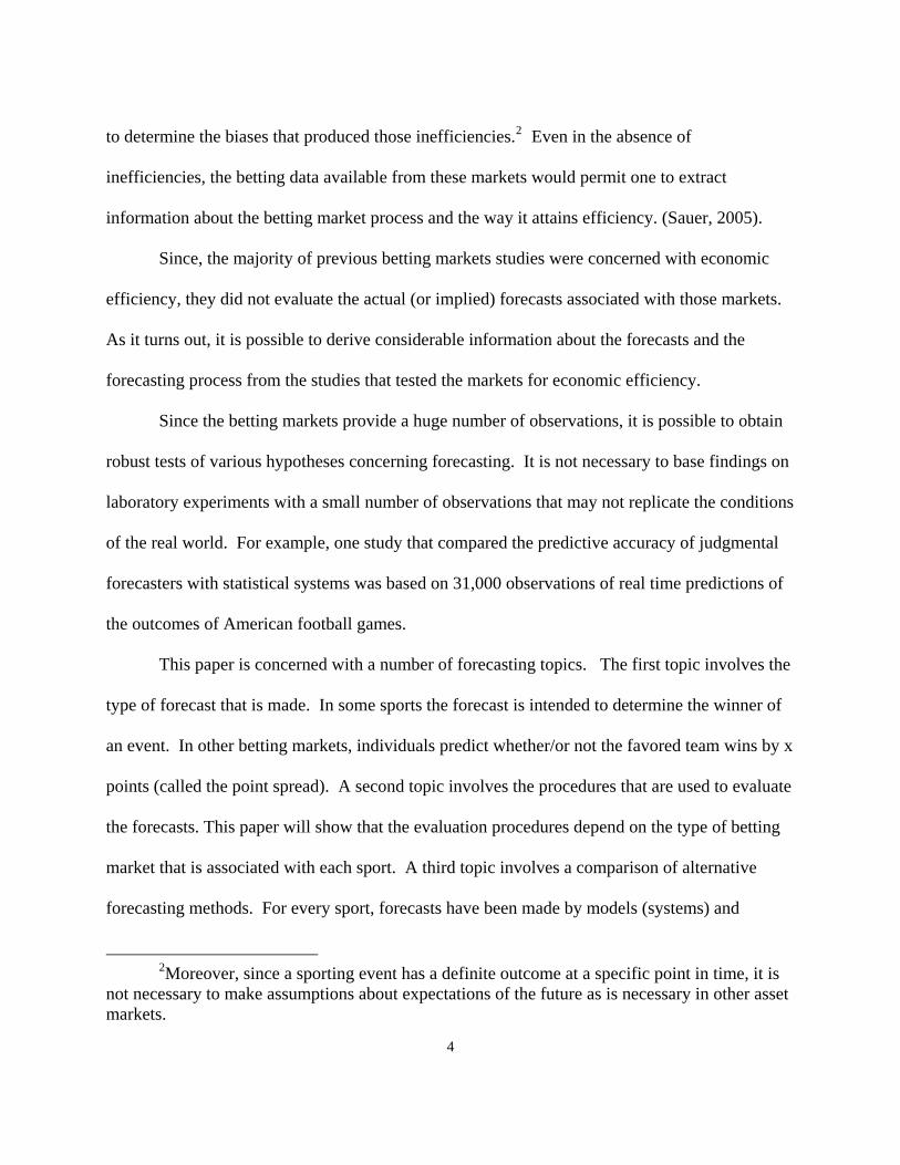
to determine the biases that produced those inefficiencies.2 Even in the absence of

inefficiencies, the betting data available from these markets would permit one to extract

information about the betting market process and the way it attains efficiency. (Sauer, 2005).

Since, the majority of previous betting markets studies were concerned with economic

efficiency, they did not evaluate the actual (or implied) forecasts associated with those markets.

As it turns out, it is possible to derive considerable information about the forecasts and the

forecasting process from the studies that tested the markets for economic efficiency.

Since the betting markets provide a huge number of observations, it is possible to obtain

robust tests of various hypotheses concerning forecasting. It is not necessary to base findings on

laboratory experiments with a small number of observations that may not replicate the conditions

of the real world. For example, one study that compared the predictive accuracy of judgmental

forecasters with statistical systems was based on 31,000 observations of real time predictions of

the outcomes of American football games.

This paper is concerned with a number of forecasting topics. The first topic involves the

type of forecast that is made. In some sports the forecast is intended to determine the winner of

an event. In other betting markets, individuals predict whether/or not the favored team wins by x

points (called the point spread). A second topic involves the procedures that are used to evaluate

the forecasts. This paper will show that the evaluation procedures depend on the type of betting

market that is associated with each sport. A third topic involves a comparison of alternative

forecasting methods. For every sport, forecasts have been made by models (systems) and

2Moreover, since a sporting event has a definite outcome at a specific point in time, it is

not necessary to make assumptions about expectations of the future as is necessary in other asset markets.

5

experts. In some sports, it is also possible to analyze a forecast that is made by the market. The

final topic is to determine whether the forecasts are biased and, if they exist, the sources of the

biases.

These topics will be discussed on a sport-by-sport basis in the next few sections. Then

we will undertake a cross sport comparison to determine whether the results for individual sports

yield valid generalizations about sports forecasting. Finally, we compare the findings from

sports forecasts with the profession’s generally accepted beliefs and see whether they are

consistent.

I. The Sports Gambling Market and Forecast Evaluation Procedures

Given that the data are generally associated with and obtained from the gambling market,

it is first necessary to discuss how the markets are structured. The gambling markets are

constituted differently from sport to sport. In horse racing, baseball and soccer the bet involves

picking a winner, and the market quotes odds that a particular horse or team will win. As an

example, if there were only two teams and there were no commissions, the odds on the underdog

might be 2 to1 and the odds on the favored would then be 1 to 2. A winning bet on the underdog

will pay $2 for every $1 that was bet and the payoff to the favorite would be 50 cents for every

dollar bet. In either case, the winner would also have the original bet returned; in our example

the payoffs would be $3 and $1.50, respectively for every dollar bet.

In markets where odds are quoted, it is not possible to determine whether forecasters

correctly predicted the winners when there are more than two competitors. Rather the

forecasting evaluation is based on a comparison of the ex ante probabilities and the ex post ratio

6

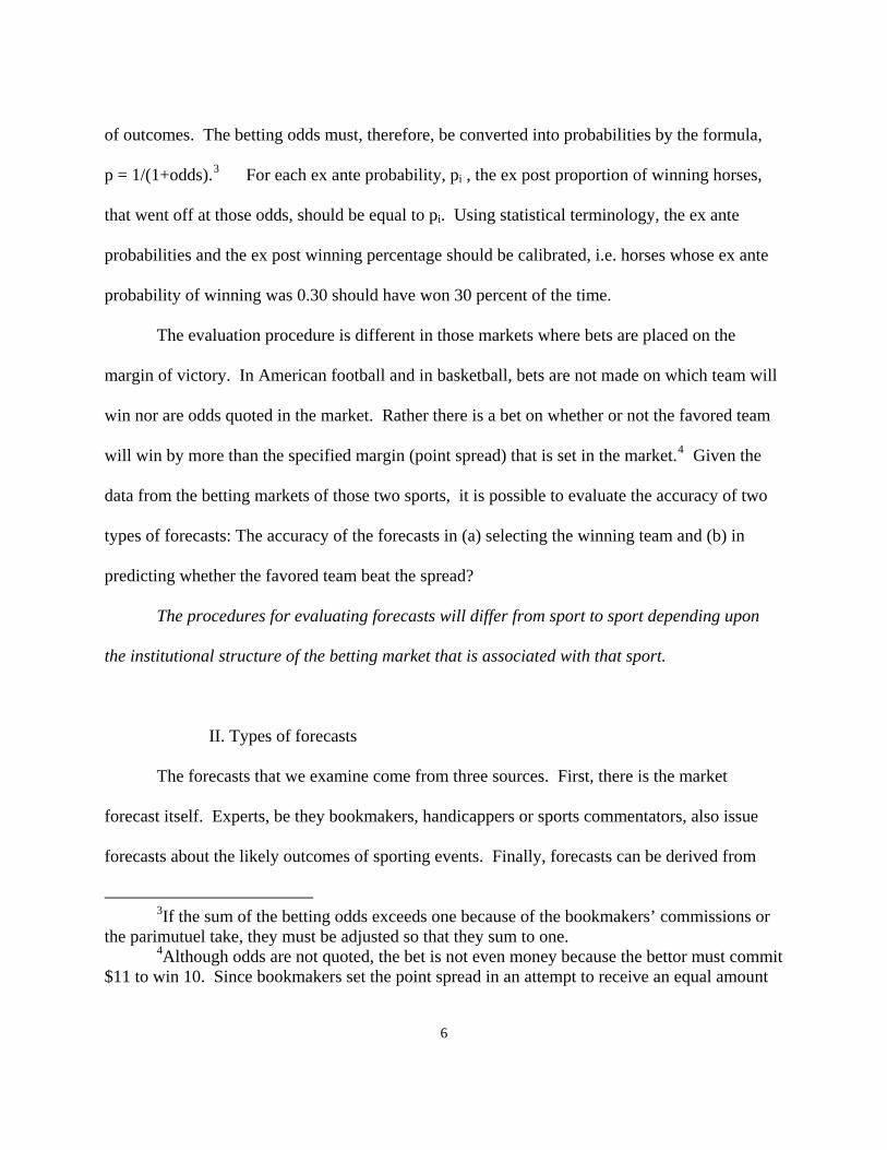
of outcomes. The betting odds must, therefore, be converted into probabilities by the formula,

p = 1/(1+odds).3 For each ex ante probability, pi , the ex post proportion of winning horses,

that went off at those odds, should be equal to pi. Using statistical terminology, the ex ante

probabilities and the ex post winning percentage should be calibrated, i.e. horses whose ex ante

probability of winning was 0.30 should have won 30 percent of the time.

The evaluation procedure is different in those markets where bets are placed on the

margin of victory. In American football and in basketball, bets are not made on which team will

win nor are odds quoted in the market. Rather there is a bet on whether or not the favored team

will win by more than the specified margin (point spread) that is set in the market.4 Given the

data from the betting markets of those two sports, it is possible to evaluate the accuracy of two

types of forecasts: The accuracy of the forecasts in (a) selecting the winning team and (b) in

predicting whether the favored team beat the spread?

The procedures for evaluating forecasts will differ from sport to sport depending upon

the institutional structure of the betting market that is associated with that sport.

II. Types of forecasts

The forecasts that we examine come from three sources. First, there is the market

forecast itself. Experts, be they bookmakers, handicappers or sports commentators, also issue

forecasts about the likely outcomes of sporting events. Finally, forecasts can be derived from

3If the sum of the betting odds exceeds one because of the bookmakers’ commissions or

the parimutuel take, they must be adjusted so that they sum to one. 4Although odds are not quoted, the bet is not even money because the bettor must commit

$11 to win 10. Since bookmakers set the point spread in an attempt to receive an equal amount

7

statistical models that are based on the fundamentals of the sports or are based on variables that

are proxies for these characteristics.

A. Market forecasts

For each sport, the largest number of forecasts come from the betting market. The

market forecast is either the final odds that a team will win or the final point spread. As

indicated above, these forecasts can be analyzed in several different ways, depending on whether

odds or point spreads are quoted. Nevertheless, it is always possible to test for the existence of

biases and to determine whether the market forecasts were more accurate than those of other

forecasting methods.

B. Models5

In order to predict the outcome of sporting events, different types of models can be

constructed. At the most disaggregated level, it is possible to predict the outcome of a game by

modeling the effects of every play. (For baseball see Bukiet et al.,1997 and Sauer, 2005; for

soccer see Carmichael et al., 2000). At a more aggregative level, production functions are used.

These functions focus on the fundamental factors that determine the outcome of a game. On

offense it is the factors that determine the number of points or runs scored; on defense the factors

that determine the number of points or runs allowed. The model that is used to forecast the

outcome of a game is then based on the differences in the fundamental characteristics of the two

teams.

An alternative statistical procedure is to construct a power score or index that is a proxy

of money on both sides of the bet, the deviation from the even money bet represents the bookmakers’ commission.

8

for these fundamental characteristics or the latent skills and strengths of the teams. Such a model

merely uses the difference in runs ( points, goals) scored as a predictor. Then there are models

that use power scores based on relative performance as the independent variables. The focus of

these models is exclusively on the relative number (and margins) of victories of the competing

teams and the time trend in this relationship. For example, the New York Times created power

scores for every NFL team that summarized each team’s relative performance in previous games.

It was based on the winning percentage of each team, its margin of victory, and the quality of its

opponents. Similar measures, that include the strength of schedule, have been constructed for

other sports. These power scores can be transformed further into ordinal rankings. ( Boulier and

Stekler, 2003).

C. Experts

Finally, we have predictions made by individuals (experts) who may or may not reveal

their methods. Some of these experts are sports writers, editors of newspapers or sports

magazines, or sports commentators on the major television networks; others are tipsters . The

odds makers in the betting markets and the track handicappers should also be considered experts.

III. What has been forecast?

The literature with which we are concerned has examined economic efficiency issues in

virtually every sport, but the emphasis has been on the outcomes of horse races and of baseball,

football, basketball, and soccer games. There are also forecasts about the winners of

tournaments such as the NCAA basketball championships and the winners of the championship

5It should be noted that many of the models that have been estimated and that are

9

of particular leagues. We present the methodologies and results for each sport separately and

then provide a cross-sport summary in order to generalize the findings.

A. Horse Racing

Sauer (1998) and Vaughan Williams (1999) have surveyed the major studies that

analyzed the outcomes of horse races. While the major emphasis of these studies was on the

economic efficiency of the betting markets, these analyses provided insights that can have

general applicability to all fields of forecasting. The observed inefficiencies provide information

about the biases that exist. Moreover, the results suggest that it is even possible to model the

outcome of horse races. These statistical models take into account the quality of the competition

that occurs during a race.

1. Betting Market

The results indicate that the market can distinguish among horses of different quality.

With a particular exception, the subjective probabilities obtained from the odds rank of the

horses are well calibrated with the observed frequency of wins. (Sauer, 1998, pp. 2035 and

2044). This indicates the obvious presence of individuals who are informed forecasters and can

predict the outcomes of horse races.

The exception to the aforementioned calibration occurs at the extremes of the odds

distribution. Most studies of horse racing in the US yield a result that has been called “ the

favorite- long shot bias”. This means that in the parimutuel market, an insufficient amount is bet

upon the horses that are favored to win and an excessive amount is bet on the long shots, thus

discussed in this paper have never been used in forecasting beyond the period of fit.

10

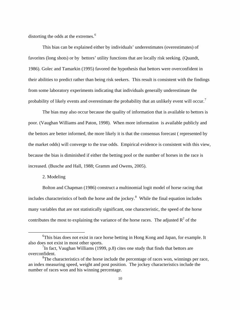
distorting the odds at the extremes.6

This bias can be explained either by individuals’ underestimates (overestimates) of

favorites (long shots) or by bettors’ utility functions that are locally risk seeking. (Quandt,

1986). Golec and Tamarkin (1995) favored the hypothesis that bettors were overconfident in

their abilities to predict rather than being risk seekers. This result is consistent with the findings

from some laboratory experiments indicating that individuals generally underestimate the

probability of likely events and overestimate the probability that an unlikely event will occur.7

The bias may also occur because the quality of information that is available to bettors is

poor. (Vaughan Williams and Paton, 1998). When more information is available publicly and

the bettors are better informed, the more likely it is that the consensus forecast ( represented by

the market odds) will converge to the true odds. Empirical evidence is consistent with this view,

because the bias is diminished if either the betting pool or the number of horses in the race is

increased. (Busche and Hall, 1988; Gramm and Owens, 2005).

2. Modeling

Bolton and Chapman (1986) construct a multinomial logit model of horse racing that

includes characteristics of both the horse and the jockey.8 While the final equation includes

many variables that are not statistically significant, one characteristic, the speed of the horse

contributes the most to explaining the variance of the horse races. The adjusted R2 of the

6This bias does not exist in race horse betting in Hong Kong and Japan, for example. It

also does not exist in most other sports. 7In fact, Vaughan Williams (1999, p.8) cites one study that finds that bettors are

overconfident. 8The characteristics of the horse include the percentage of races won, winnings per race,

an index measuring speed, weight and post position. The jockey characteristics include the number of races won and his winning percentage.

11

equation is .09 indicating that the equation explains 9% more than the null that each horse has an

equal chance of winning.

Expanded versions of this multinomial logit model improve the explanatory power of the

equations, with most of the new variables significant and the adjusted R2 exceeding 12%.

(Bentner, 1994;Chapman, 1994). While the final betting odds have even more explanatory

power, a combination of the model and the market odds improves upon both.9 This finding is

consistent with the results obtained from the non-sports forecasting literature which indicates that

combining forecasts usually improves accuracy.

3.Experts

Figlewski (1979) examined the forecasting record of a number of individuals who

handicapped horse races. While the handicappers were successful 28.7% of the time in selecting

the horse that would win the race, the favorite, as measured by the betting odds, won 29.4% of

the time. Both the track-odds and the handicappers improved over the null that all horses had an

equal probability of winning, but combining the handicappers’ selections with the market odds

did not significantly improve forecasting accuracy.10 In Britain, the odds in the handicapper’s

morning line were also less accurate in predicting the probability of winning than were the final

market odds.(Crafts, 1985).

The experts also displayed the favorite-longshot bias. Snyder (1978) found that the

favorite-long shot bias of official race track handicappers and newspaper forecasters was greater

than that of the general public. Lo (1994) showed that the favorite-longshot bias associated with

9However, in a real time situation an individual might not have the time and thus be in a

position to use the final odds in combination with the model before placing a bet.

12

the handicappers’ morning line odds was even larger than that of the final odds of the betting

market.

4.Summary

a. The market odds and the frequency of wins are calibrated except for the favorite-

longshot bias. However, this bias is not observed universally.

b. Models can explain some of the variance of horse races. Combining models with

market odds improves accuracy.

c. The odds provided by experts are better than those obtained by chance but not as

accurate as the betting market odds.

d. Experts displayed even more favorite-longshot bias than the final market odds.

B. Baseball

There is so much information about baseball, that it is surprising how few forecasts are

available for analysis. There are a number of models that have estimated the importance of the

offensive and defensive factors that determine the outcome of a game, but forecasts from these

models have not been published in the open literature.11

1. The betting market

Bets in this market are made on the outcome of a game. Consequently, like the horse race

betting market, the analysis is based on odds which can then be converted into probabilities, but

the odds are not quoted directly. The bookmaker quotes, a line, +140, -150 for example. This

10Bird and McCrae (1987) found that the odds of Australian bookmakers, who could be

considered experts, were fully incorporated into the racetrack odds.

13

means that the winner of a $100 bet on the underdog team would win $140, while someone

betting on the favored team would bet $150 to win $1. The difference is the commission. From

these odds it is possible to calculate the betting market’s subjective probability that the underdog

will win. The probability is calculated at the midpoint of the line, i.e. 1/(1.45 +1) = 0.41 . This

subjective probability can then be compared with the percentage of times that the underdog won

when those odds were quoted. If the subjective probabilities are calibrated with the observed

probabilities, the forecasts would be considered rational.

Three studies examine the relationship between these subjective and observed

probabilities. Woodland and Woodland (1994, p.275; 1999, p.339) and Gandar et al. (2002,

p.1313) all indicate that the odds are related to the observed outcomes, but the relationship is not

strictly monotonic.12 In order to test whether the forecasts were rational, Woodland and

Woodland (1994) regressed the objective probabilities on the subjective odds. They obtained

mixed results that were dependent on the method of estimation. They argued that betting in

baseball yielded a reverse favorite-underdog bias, with underdogs underbet. Gandar et al. made

a minor correction to the Woodland-Woodland methodology and found that rationality was not

rejected, and if there were any bias, it was very slight.

2. Modeling

Many of the basic models of a baseball game consider either the characteristics of the

offense to determine the number of runs scored or the qualities of the pitching staff in permitting

runs to be scored. Thus Porter and Scully (1982) estimate a production function based on a

11Individuals may have used these models in deciding whether to place bets about the outcome of games, but these data are not readily available.

14

team’s slugging average and its strike out to walk pitching ratio.13 Other models provided more

detail about baseball’s offense and pitching; for example Bennett and Flueck (1983) examined

various characteristics of offense14 to determine the number of runs that would be scored but did

not make explicit predictions with their model. The model was estimated using data from the

1969-1976 seasons. It was then reestimated by sequentially eliminating one year’s data from the

sample using the data of the remaining seven years. While the adjusted correlation coefficients

of those eight regressions did not differ significantly, the coefficients of some of the variables did

display considerable variation.

Rosner et al. (1996) estimated relationships that measured pitcher performance and

determined the number of runs that would be scored in each inning. They were able to do this

because play-by-play data have been available for all Major League Baseball games since 1984.

An adjusted negative binomial distribution was fit to the data to explain the number of batters

that a particular pitcher would face. The number of runs that will be scored is a complex

function of two distributions: this negative binomial distribution and a conditional distribution of

the number of runs that score given that the pitcher has faced a specified number of batters.

(Rosner et al. 1996, p.352.) Other studies include Malios (2000) who listed the factors that

determined offensive and pitching performance, and Turocy (2005) who added a speed variable

to the conventional production function. None of these models produced forecasts that could be

12The QPS statistic also known as the Brier score could have been calculated and decomposed to determine the degree of calibration.

13This model was not used as a predictor but rather was employed to measure the relative performance of baseball managers. Horowitz (1994) uses a power score variant of this production function (runs scored/ runs allowed) in a similar analysis of managerial performance. See Ruggiero et al. (1997) and Horowitz (1997) for a further discussion of this subject.

14These variables included the various types of hits, walks, types of outs, etc.

15

evaluated.

On the other hand, Bukiet et al. (1997) modeled each at-bat as a 25x25 transition matrix

that explained all of the alternatives that might occur. Markov chains were then used to predict

team performance based on the characteristics of each batter. This model was used to predict the

actual number of games that all of the teams in the National League would win in 1989. While

the model failed to predict one of the two divisional winners and the number of runs that were

scored was underestimated, the Spearman Rank Correlation between the predicted and actual

number of games that each team won was .77. (Authors’ calculations).

There are two other models that were used to predict National League divisional winners.

Barry and Hartigan (1993) used a binary choice model to calculate the probability that in 1991 a

National League team would win its division. The model was based on the strength of the teams

as the season progressed with greater weight placed on the most recent sequence of games as

well as the teams’ home field advantage. Using simulations, the model successfully showed that

Atlanta’s probability of winning its division was increasing as the season progressed. Finally,

Smyth and Smyth (1994) based their predictions of division winners and relative standings on

the payrolls of each of the teams in each division and league. They found that the rankings

within a division were correlated with the teams’ payrolls.15

3. Experts and Experts vs. Models

Despite all the predictions that are made every year by experts about the relative expected

performance of the Major League teams, we found only one study that examined the quality of

15Szymanski (2003, p. 1154) presented similar results for soccer. He showed that, within

each league, the winning performance of a team was associated with the relative size of the teams’ payrolls. Forrest et al. (2005a) use payrolls as a measure of team quality.

16

those forecasts. Smyth and Smyth (1994) found that the experts’ forecasts were better than

random guesses. However, the predictions of those experts were not significantly different from

those based on the rankings of teams’ payrolls.

4. Summary

a. The market odds are calibrated with the observed ratios of outcomes, but there is some

debate about the possibility of a reverse favorite-longshot bias.

b. Many models that explain various aspects of a baseball game have been estimated, but

they have not been used to make forecasts.

c. There is one study that examined the forecasts of experts. The experts’ predictions

were better than random, but not different from models that used payrolls as the

predictor.

C. Football

The forecasts about the outcomes of professional and college football games, like those

from other sports, come from the betting market, statistical systems, and experts. Unlike horse

racing and baseball where odds are used in establishing the payoff to a bet that involves selecting

a winning horse or team, football bets do not involve selecting the winning team. Rather the bet

is whether or not the favored team beats the underdog by a margin (number of points) specified

in the bet. This margin is called the point spread. If an individual bets that the favored team will

beat the underdog by more than this spread, the bettor only wins if the favorite is victorious by

more than this number of points. Someone betting on the underdog can win if there is an upset

and the favored team loses or if the favorite wins by less than the specified number of points.

17

Every bettor pays $11 for a $10 payoff. The difference is the bookmaker’s commission also

known as the vigorish. Given this commission, a bettor must be right at least 52.4% of the time,

just to break even. (Sauer, 1988, p. 211 )

While the betting market is not concerned with selecting the winning team, it is possible

to use the data about the spread to determine whether the market accurately predicts who will

win. Thus, our analysis of the betting market examines two questions: (1) How frequently does

the team that is favored to win actually win? and (2) Are there any observed biases in the spreads

that were published just before the game was played?

1.Betting Market

a. Winners

The focus of the previous analyses have been whether the betting market involving NFL

games was economically efficient. With a few exceptions, the studies have not considered the

forecasting accuracy of the market in predicting the winners of games. Stern (1991)

demonstrated the difference between the winning margin and the point spread was normally

distributed with mean zero and a standard deviation equal to 14. He then used the observed

spreads in simulations to determine how the teams would have done in the 1984 season. The

results were mixed. While 5 of the 6 division winners were identified, only 1 of the 4 additional

playoff teams was selected by the model.

Boulier and Stekler ( 2003) and Song et al. (2007) showed, that in every year from 1994-

2001, the betting market correctly predicted the winner of NFL games at least 63% of the time.

The average over this time period was about 65%. In fact, in selecting the winners of games, the

betting market was the most accurate forecasting method in every year. We tabulated the

18

relationship between the point spread and the ex post winning percentage of the home team.

Table 1 indicates that the ex post winning percentage is positively related to the ex ante spread,

but the increase is not monotonic.

b. Point spread

In analyzing the market’s performance relative to the spread, the main question is: Are

there any observed biases? The overwhelming majority of the evidence indicates that the betting

market is efficient in the sense that, on average, there is no profitable betting strategy against the

spread. The traditional method for determining whether a forecast is unbiased is to run the

regression:

A = a + bF + e, (1)

where A is the actual value and F is the forecast. If the joint null hypothesis that a = 0 and b =1

is rejected, the forecasts are biased. In the football betting market, the equivalent equation is:

DP = a +bPS + e, (2)

where DP is the difference in the game score ( actual points) and PS is the betting market point

spread.16 If the forecast is unbiased, on average, the difference in the point scores will not differ

significantly from the point spreads. Most studies do not reject the null hypothesis that a = 0

and b =1, but the explanatory power of the equation is usually low indicating that there is

considerable unexplained variation.

On the other hand, Gray and Gray (1997) use a different method to test the hypothesis

that the forecasts are efficient. They estimate a probit where the dependent variable is whether

19

the team beat the spread or not.17 They find that two variables, whether a team plays at home

and whether it is a favorite, are jointly significant. If the market had provided an efficient

forecast, neither variable should have had any explanatory power.18

Since there is a considerable amount of unexplained variability, forecasting biases and

profitable betting strategies may exist. We are concerned only with the forecast biases. Vergin

(2001) argued that bettors ( forecasters) were subject to an overreaction bias, i.e. they overreact

to the most recent positive information and undervalue other data. “For example, if a team won

a game by a very large margin in a given week, the betting public would tend to overrate the

team in the following week.” (Vergin, 2001, p. 499).19 Vergin examined a number of ways that

bettors ( forecasters) could have reacted to recent information. He found that, in most cases,

over 15 seasons, the bettors had displayed a bias in interpreting recent positive data. Gray and

Gray (1997) also found that the market overreacted to the most recent information.20

The forecasting literature has also analyzed the way that individuals interpret

information. Kahnemann and Tversky (1982) had argued that individuals place too much

emphasis on new information, but some experimental data suggested the opposite: people anchor

on a past observations and place too little emphasis on new information. (Andreassen, 1987,

1990) The data from the football betting market seem to favor the former view.

16Both the scores and the point spreads are usually constructed on a home team minus

away team basis. 17 A probit places less weight on outliers than OLS does. 18There is, however, a controversy about the appropriate way to jointly test for home

team bias and underdog bias. (Golec and Tamarkin, 1991; Dare and MacDonald, 1996; Dare and Holland, 2004).

19Vergin and Scriabin (1978) were also concerned with this issue.

20

2.Models

The many statistical systems that are designed to predict the margin of victory of NFL or

college football games are estimated in different ways.21 Zuber et al., (1985) and Sauer et al.,

(1988) derived models using the fundamental characteristics of a team’s offense and defense to

explain the margin of victory. Those models correctly predicted a margin of victory that would

have been profitable 59% of the time for games played in 1983, but the success rate was only

39% in 1984.22 Dana and Knetter (1994) developed a dynamic model using point score indices

as a measure of the abilities of the teams but the accuracy ratio of the model was generally less

than 50%.

Other models are based on power scores that summarize the latent abilities of the football

teams. Variants of these power scores have been used in forecasting both the outcomes of

football games and the margins of victory. Harville (1980) found that in the 1971-77 seasons the

betting market, with a 72% success rate in selecting the winner, was more accurate than his

statistical procedure, which was right 70% of the time.23 Boulier and Stekler (2003) used the

power scores published in the New York Times and analyzed the forecast: the team with the

20In addition, Gray and Gray observed that the market had a slight overconfidence in the

favorite’s ability to cover the spread. In the 1976-94 seasons, that team won by slightly less than the market had expected.

21Song et al. (2007) used information from 32 systems that provided information on the Internet.

22The papers did not indicate the number of times that the model predicted the winners of each game, but the models explained 73-81% of the variance of the score differentials for the two NFL seasons.

23These success rates are higher than the accuracy that has been observed in more recent seasons. One explanation is that more ties occurred in the earlier seasons and Harville counted a tie as ½ of a successful forecast. Harville did not report the methods’ record in betting against the spread.

21

higher power score would win. These forecasts had an accuracy ratio of 61%, less than that of

the betting market which achieved 66% accuracy and only comparable to a naive forecast that

the home team will win.

An intensive evaluation of the forecasting record of statistical systems indicated that they

had a 62% average accuracy ratio in picking the winners of the games played in the 2000 and

2001 NFL seasons. ( Song et al., 2007). This ratio was comparable to the record of experts but

less than the 66% accuracy of the betting market. Every system had a success rate of at least

50% and the ratios for all but one system were significantly different from those that could have

occurred by chance.24 In forecasting against the betting spread, most systems, however, were

not even as accurate as the naive forecast of flipping a coin.

3. Experts

We found information about two types of experts: bookmakers25 and sports

commentators (analysts). In NFL games the bookmakers .........AVERY AND CHEVALIER.

In the college football betting market, the bookmakers set an opening line that was biased against

the favorite team, but the closing spread was less biased. (Dare et al., 2005).

Song et al. (2007) undertook a comprehensive analysis of the other group of experts and

examined the ability of sports commentators to predict either the outcome of NFL football games

or the margin by which a team was expected to win. That study used the forecasts of 48 experts

who predicted which team would win and an overlapping ( but not identical) set of 52 forecasters

who made selections against the betting line. All told, the forecasts of 70 experts were analyzed.

24 The test was based on the binomial distribution and a 5% level of significance.

22

Based on this sample of nearly 18,000 forecasts for the 2000 and 2001 seasons, Song et al.

concluded that experts predicted the game winner approximately 62% of the time; this was the

same accuracy ratio as the statistical systems achieved, but was less than the betting market’s

66%. Similarly, the accuracy ratios of both the experts and systems in forecasting against the

betting line was 50%. On average the experts did worse than using the naive model of flipping a

coin.

Less comprehensive studies yield similar findings. Boulier and Stekler (2003) report

that the sports editor of the New York Times selected the winner of the games during the 1994-

2000 seasons 60% of the time. Even earlier, Pankoff (1968) showed that experts’ accuracy in

forecasting whether a team would beat the spread ranged from 48% to 56%.

4. Summary

a. The market correctly picks the winner of a game about 2/3 of the time. This record is

better than that of the experts and systems.

b. The null that the point spread is an unbiased predictor of the margin of victory is

generally not rejected.

c. Models are successful in predicting winners but they are not as accurate as the betting

market.

d. Models and experts are equally good both in forecasting winners and in predicting

against the spread. The predictions against the spread are not significantly better than

chance.

D. Basketball

25For information about the process of setting the opening line ( spread ) on football

23

1. Betting Market

The studies that have analyzed the basketball betting market have not found any

significant biases. There is a slight but insignificant underestimate of the home court advantage,

(Brown and Sauer 1993a) and large favorites may be over bet. (Paul and Weinbach, 2005a,

2005b).

The major forecasting issues of interest in the basketball betting market are (1) the

absence or presence of the “hot hand” phenomenon and (2) the use of information in this market.

The “hot hand” is a belief that a team that wins a game is more likely to win the next game and

indicates that forecasters believe that these events are not independent but rather are positively

autocorrelated. Camerer (1989) argues that the hot hand is a myth and that bettors have a

misunderstanding of random processes, especially with small samples. Brown and Sauer

(1993b) build a model based on teams’ abilities and streak dummies in order to test this

hypothesis. They conclude that the hot hand belief is embodied in the point spread and is,

therefore, an important effect.26 However, they were not able to determine whether, in fact, a hot

hand phenomenon existed or whether it was a myth and bettors were misperceiving the real

process and thus displaying a cognitive bias.

Using changes in the betting line, it is possible to infer the role that information and

informed bettors play in the betting market. Brown and Sauer (1993) and Gandar et al (1998,

2000) examine these questions from different perspectives. Brown and Sauer first estimate a

model based on a proxy for fundamentals: the points scored by the two teams that play against

each other. This model explains 89% of the variation in the point spread and also predicts well

games, see Schoenfeld, (2003).

24

out of sample. Brown and Sauer thus conclude that the betting market adjusts for fundamental

changes in the relative team abilities that may have occurred from one season to another.

Gandar et al. examine the differences between the opening and closing point lines for

NBA games.27 They show that frequently there are large changes between the opening and

closing quotations. These changes reflect betting sentiment that is different from that of the

bookmaker. They test a number of hypotheses, show that the opening line is not as accurate as

the closing line in forecasting the margin of victory, and conclude that informed bettors have

eliminated some of the bias in the opening line.

2. Models

Zak et al. (1979) developed a production function that represented the defensive and

offensive elements of a basketball game. The model was designed to measure the relative

contribution of each of those elements to the winning margin. Each team’s productive efficiency

was then calculated. The rank of each team in terms its productive efficiency was identical to the

rank based on winning percentage in the 1976 NBA season. This method has not been

subsequently used for making forecasts.

Berri (1999) used a similar model that was designed to measure the contribution of

individual players to a team’s wins. Rather than directly predicting a team’s wins, each player’s

contribution towards his team’s wins were summed. The ranking obtained by summing the

26Also see Paul and Weinbach (2005b). 27Gandar et al. (1998) examine the winning margin ( the difference in the scores of the

two teams) while Gandar et al. (2000) analyze the totals betting market (the sum of the scores of the teams). The opening line is set early in the day that the game is played and the closing line is established just before the game begins. Thus it is not likely that much new information about the teams will have become available during the course of the day.

25

contributions of each player to team victories was remarkably close to the ranking based on the

teams’ actual won-lost records in the 1997- 1998 season. The Spearman Rank Correlation was

.986 (Authors’ calculations).

Other modeling approaches did not construct production functions but rather used proxy

variables that measured the latent skills or strengths of each team. The margin of victory in a

contest between two teams was considered a measure of the comparative strengths of the two.

(Brown and Sauer, 1993; Harville and Smith, 1994; Oorlog, 1995; Kaplan and Garstka, 2001;

Harville, 2003). On the other hand, if two teams that had not played each other previously were

to meet, it would be impossible to measure the comparative strengths of those opponents. This is

a particular problem in trying to forecast the outcomes of college basketball (and football)

games, because no team plays every other team.

Statistical scoring systems have been developed to overcome this problem. As an

example, Sagarin has developed a system that can be used to predict the expected scoring by any

two teams. This system is based on the number of victories of each team, the strength of the

teams that were defeated, the margin of victory adjusted for blowouts, and an adjustment for the

home court advantage.28

Alternatively, in a tournament, the seedings, which are obtained from a statistical scoring

system, of the teams can be used as a predictor. Since 1985, the NCAA has selected 64 college

basketball teams to participate in a tournament to select a national championship. The 64 teams

28The difference between two teams’ Sagarin ratings is a good predictor of the margin of

victory. (Carlin, 1996).

26

are divided into four regional tournaments of 16 teams that are ranked from 1 through 16.29

Boulier and Stekler (1999), Caudill and Godwin (2002), Kaplan and Garstka (2001), and

Harville (2003) all found that the difference in ranks predicted the winner around 70% of the

time. However, their statistical models differed.

Boulier and Stekler (1999) used a probit based solely on the difference in ranks. Caudill

and Godwin (2002) developed a heterogeneous skewness model that takes into account not only

the difference in ranks but also the level of the seed. Thus the probability that a Number 1 seed

beats a Number 5 seed is greater than the probability that a Number 5 seed beats a Number 9

ranked team. Finally, Harville (2003) constructed a modified least squares ranking procedure

based by placing a limit on the margin of victory and then compared the forecasts of the model

solely with the difference in ranks. (Also see Schwertman et al., 1991, 1996; Carlin, 1996).

The accuracy of forecasts based on ranks has been compared with that of other methods.

Kaplan and Garstka (2001) found that forecasts based on picking the higher seeds was slightly

more accurate than using the betting market and that forecasts based on the Sagarin system were

superior to both. Harville (2003) then compared the forecasting accuracy of his statistical

method with (1) forecasting that the higher seed will win and (2) the betting market. The

statistical procedures were the most accurate in forecasting the winners of the 2000 NCAA

tournament, but there was little difference between forecasts based on ranks and the betting

market. Kaplan and Garstka and Harville have been the only authors who have found that

forecasts obtained from the market were not more accurate than those obtained from either

29 The seeds are determined from a statistical scoring system, the RPI, called the ratings

percentage index. It gives weights of .25, .50, and .25 to the team’s winning percentage, the

27

experts or statistical systems.30

3. Experts

While there are no studies that have directly examined the forecasts of experts in

predicting the outcomes of basketball games, there is one piece of indirect evidence. The

bookmakers who set the opening line or point spread can be considered experts. The evidence is

that the opening line that is established by the bookmakers is somewhat less accurate than the

closing line established by the betting market.31 ( Gandar, et al., 1998). This indicates that

experts are not as accurate as the market in forecasting the winning margins. However, this

result does not imply that the experts exhibit a bias, because the changes between the opening

and closing lines seem to be normally distributed around zero ( no change). (Gandar et al., 1998,

Table IV, p. 395).

4. Summary

a. The basketball betting market does not have any observed biases; the market moves to

eliminate the early biases of the bookmakers.

b. Many models of basketball games have been estimated, but except for games played in

the NCAA tournaments there have been few forecasts.

c. The only evidence that we have about experts is that the bookmakers’ opening line is

less accurate than the final spread.

winning percentage of its opponents, and winning percentage of the opponents’ opponents, respectively.

30 Harville also found that there was no significant difference between the market and statistical systems in the football bowl games played after the 2001 regular season.

28

E. Soccer

Gambling in soccer is based on odds, but this betting market is different from those that

have been analyzed above. The bookmakers set the odds at the beginning of a week and do not

change them during the betting period. While some studies have tested for bias and

inefficiencies, the focus of the literature relating to this sport has been on statistical procedures

and the performance of these models relative to the bookmakers’ odds.

1. Betting Market and Bookmakers

In one of the few studies that searched for biases, Cain et al. (2000) showed that there

was a favorite- longshot bias, similar to that found in horse racing, in the soccer betting market.

Many studies have found that models contained information that was not embodied in the odds.

(Pope and Peel, 1989; Kuypers, 2000; Goddard and Asimakopoulos, 2004; Dixon and Pope

(2004) These findings suggests that the bookmakers’ odds were inefficient.

2. Models

The modeling has been done at three levels. In the production function approach

variables that are associated with attack and defense are embodied in the model. A second

approach is to model each team’s goal scoring abilities and then predict which team will win

based on the difference in the predicted number of goals. Finally, discrete choice models based

on past performance are used to directly predict the probabilities of the home team winning,

drawing or losing.

In the production function approach, Carmichael et al. (2004) estimated the effects of

specific types of plays on the difference in the number of goals scored by the two teams. Their

31 While the results are significantly different, the differences are too small to be

29

equation was able to capture the relative performance of teams in the English Premier league,

but they did not make any forecasts beyond the period of fit.

The Poisson distribution is an alternative model for predicting the number of goals that

teams will score. Dixon and Coles (1997) show that this distribution provides a good fit to the

score data for the 1992-95 seasons, but they add attack and defense parameters to the basic

model of Maher (1982).. Moreover, they permit the parameters to vary to reflect changes in

team strength that may have occurred over time. The probabilities obtained from the Dixon-

Coles model are similar to those of the bookmakers (as derived from the odds).32 ( Dixon and

Pope, 2004). The model of Cain et al. differed from that of Dixon-Coles for two reasons. It used

the negative binomial distribution33 to model the number of goals scored, and the independent

variables were the win-lose odds prices quoted by the bookmakers rather than proxy attack-

defense variables. The Cain et al. model predicted the total number of goals each team scored

and yielded probability forecasts that approximated the observed distribution of particular scores.

Since the abilities and performance of teams can change over time, some models have

become dynamic to capture these effects. Dixon and Coles were among the first to incorporate

dynamic factors into their model. Crowder et al. (2002) derive an approximation to the Dixon-

Coles model, show that the two models yield similar results, but the success ratio associated with

the prediction, home team will win, is only around 50%.

The Bayesian dynamic model of Rue and Salveson (2000) yielded model likelihood

economically meaningful.

32Dixon and Coles do not provide a detailed evaluation Nor do they compare their predictions with a naive forecast that the home team wins 46%, draws 27%, and loses 27% of the time.

33The Poisson distribution is a limiting case of the negative binomial.

measures that were very similar to the bookmakers’ odds. Moreover, they used a Markov chain

Monte Carlo retrospective analysis to predict the posterior final rankings of the teams in the

English Premier League. The relationship between the actual and predicted rankings in the

1997-1998 season was not perfect. The model forecast that Manchester United had a 43%

chance of being the highest ranked team; it finished second to Arsenal that had been given a 25%

chance. Nevertheless, the model correctly selected the top four teams in the League.

The discrete choice models were based on ordered probits that included a variety of

explanatory variables. Kuypers (2000) included the bookmakers’ odds as well as some

performance variables in his model. The win ratios of the two teams playing the match were

included as independent variables in the model of Goddard and Asimakopoulos (2004). Neither

study compared the models’ predicted probabilities with the outcomes, but both indicated that

there was little difference between the models’ and bookmakers’ probabilities.

3. Experts

We have data that evaluates the forecasts of two types of experts. The first is the group

of tipsters who write for newspapers;34 the second consists of the bookmakers who provide the

fixed odds. The evidence is that the tipsters’ forecasts have little value and that they do not

process public information properly. (Pope and Peel, 1989; Forest and Simmons, 2000).

On the other hand, Forrest et al. (2005) demonstrate that there is virtually no difference

between the accuracy of the forecasts of the odds-makers and those obtained from a complex

statistical model. This result is consistent with previous results because Kuypers (2000, Table 2,

34Andersson et al. (2005) evaluated the predictions of the outcome of the 2002 World

Cup matches made by individuals who had familiarity with soccer. The participants were called

30

p.1359) had shown that the bookmakers’ odds, when converted into probabilities are closely

related to the objective ratios of the outcome of the events. (Also see Goddard and

Asimakopoulos, 2004).

4. Summary

a. There is no serious bias in the fixed-odds soccer betting market, but there are some

inefficiencies.

b. Many types of models involving soccer have been estimated and have generated

predictions that are comparable to those of the bookmakers.

c. The tipster forecasters were not very valuable, but there was no difference between the

forecasts of bookmakers and those of a sophisticated statistical model.

IV. Results

A. Cross-Sport results

So far we have considered the forecasting procedures and results only on a sport by sport

basis. The results relating to the various sports are so similar that the conclusions have to be

considered robust.

1. In every sport, except for horse racing, the market forecast is unbiased. The bias in

horse racing occurs at the two extremes: favorites are underbet and long-shots are overbet, but

these results do not hold in all countries.

experts but in reality they were not “real” experts. In any event, their predictions were no better than those that could have occurred by chance.

31

2. In markets where odds are quoted, the ex ante betting probabilities and the ex post

outcome ratios are calibrated.

3.The betting spread is an unbiased predictor of the winning margins in American

football and basketball. Moreover, the betting market correctly predicted the winner of NFL

games about 2/3 of the time.

4. Models that explain the outcomes of games or matches have been estimated for all

sports. Sometimes the models were derived from the fundamental characteristics of the sport. In

other instances, variables that were proxies for these fundamental characteristics were used as

explanatory variables or discrete choice models were used.

5. The forecasts of many models were not available. However, systems correctly

predicted the winners of NFL games more than 60% of the time. This was comparable to the

accuracy of experts but less than that of the market. The soccer models were comparable in

accuracy to bookmaker odds.

6. In analyzing the forecasts of experts, it is important to realize that there are many types

of experts and that the extent of knowledge differs among the various groups. Experts who have

a financial stake in the forecast are likely to be more knowledgeable.

7. There is no evidence that either statistical systems or experts consistently outperform

the betting market.

B. APPLICABILITY OF THESE RESULTS TO FORECASTING IN GENERAL

The analysis of the sports forecasts also provided insights about the forecasting process.

Some of these results are in accord with the generally accepted views of the forecasting

32

profession; others are in conflict with those beliefs or require further research. The findings that

agree with our a priori views:

1. Forecasters correctly used information to reduce the biases that they observed. In horse

racing, more information reduced the favorite- longshot bias; the final odds in horse racing were

less biased than those of the racetrack’s handicapper; in basketball the closing spread was closer

to the margin of victory than was the opening quote. AVERY AND CHEVALIER

2. Forecasters are overconfident in their ability to predict.

3. Many forecasters have a misunderstanding of random processes as evidenced by their

belief in the hot hand.

4. Combining forecasts does improve accuracy.

C. CONFLICTING RESULTS

However, our analysis of these sports forecasts seriously conflicts with the widely held

belief that the predictions derived from statistical methods are more accurate than those of

experts. The analysis of 31000 NFL forecasts by Song et al. showed that the accuracy of the two

methods of forecasting was virtually identical. The accuracy of the statistical methods was,

however, less variable. Similarly in soccer, there was no difference between the accuracy of the

models’ and bookmakers’ forecasts.

An area that requires further research concerns the relative weight that forecasters place

on new and old information. There is a gambler’s fallacy that the next outcome, even though it

is independent of previous events, depends on events that have previously occurred. This fallacy

has been observed in horse racing studies. This is akin to placing too much weight on new

information. (Vaughan Williams, 1999, pp. 15-16). The majority of the evidence indicates that

33

forecasters overreact to new information rather than anchor on the old forecast and adjust it in

the face of the new data. On the other hand, Sauer (1998, p. 2059) reports on situations where

recent information is given too little weight relative to what is optimal.

D. MOST IMPORTANT RESULT

There is no evidence that either statistical systems or experts consistently outperform the

market. This not only agrees with the findings about economic efficiency but also with the

evidence that prediction models, in general, are the most accurate predictors in other fields. The

market price is the best predictor of the event because the market aggregates all the information

that is relevant to the event. ( Wolfers and Zitzewitz, 2004).

.

34

Bibliography

Andersson, P., J. Edman and M. Ekman, (2005), Predicting the World Cup 2002 in soccer: Performance and confidence of experts and non-experts, International Journal of Forecasting, 21, 565-576. Avery, C. and J. Chevalier, (1999), Identifying investor sentiment from price paths: The case of football betting, Journal of Business, 72, 493-521. Barry, D. and J. A. Hartigan, (1993), Choice models for predicting divisional winners in Major League Baseball, Journal of the American Statistical Association, 88, 766-774. Bennett, J. M. and J. A. Flueck, (1983), An evaluation of Major League Baseball Offensive performance models, The American Statistician, 37, 76-82. Bentner, W., (1994), Computer based horse race handicapping and wagering systems: A report, in --------------------------------------------------------------------------------------------------, 183-198. Berri, D. J., (1999), Who is ‘most valuable’? Measuring the player’s production of wins in the National Basketball Association, Managerial and Decision Economics, 20, 411-427. Bird, R. and M. McCrae, (1987), Tests of the efficiency of racetrack betting using bookmaker odds, Management Science, 33, 1552-1562. Bolton, R. N. and R. G. Chapman, (1986), Searching for positive returns at the track: A multinomial logit model for handicapping horse races, Management Science, 32, 1040-1060. Boulier, B. L., and H. O. Stekler, (1999), Are sports seedings good predictors?: An evaluation, International Journal of Forecasting, 15, 83-91. Boulier, B. L., and H. O. Stekler, (2003), Predicting the outcomes of National Football League games, International Journal of Forecasting, 19, 257-270. Brown W. O. and R. D. Sauer, (1993a), Fundamentals or noise? Evidence from the professional basketball betting market, Journal of Finance, 48, 1193-1209. Brown W. O. and R. D. Sauer, (1993b), Does the basketball market believe in the hot hand? Comment, American Economic Review, 83, 1377-1386. Bukiet, B., E. R. Harold, and J. L. Palacios, (1997), A Markov chain apporach to baseball, Operations Research, 45, 14-23.

35

Busche, K. and C. D. Hall, (1988), An exception to the risk preference anomaly, Journal of Business, 61, 337-346. Cain, M., D. Law, and D. Peel, (2000), The favourite-longshot bias and market efficiency in UK football betting, Scottish Journal of Political Economy, 47, 25-36. Camerer, C. F., (1989), Does the basketball market believe in the hot hand? American Economic Review, 79, 1257-1261. Chapman, R. G., (1994), Still searching for positive returns at the track: empirical results from 2000 Hong Kong races,-------------------------------------------------------------------------, 173-181. Carlin, B. P., (1996), Improved NCAA basketball tournament modeling via point spread and team strength information, The American Statistician, 50, 39-43. Carmichael, F., D. Thomas and R. Ward, (2000), Team performance: The case of English Premiership football, Managerial and Decision Economics, 21, 31-45. Crafts, N. F. R., (1985), Some evidence of insider knowledge in horse race betting in Britain, Economica, 52, 295-304. Caudill, S. B. and N. H. Godwin, (2002), Heterogeneous skewness in binary choice models: Predicting outcomes in the men’ NCAA basketball tournament, Journal of Applied Statistics, 29, 991-1001. Crowder, M., M. Dixon, A. Ledford, and M. Robinso, (2002), Dynamic modelling and prediction of English Football League matches for betting, The Statistician, 51, 157-168. Dana J. D. and M.M. Knetter, (1994), Learning and efficiency in a gambling market, Management Science, 40, 1317-1328. Dare, W. H. and S. S. MacDonald, (1996), A generalized model for testing the home and favorite team advantage in point spread markets, Journal of Financial Economics, 40, 295-318. Dare, W. H. and A. S. Holland, (2004), Efficiency in the NFL betting market: Modifying and consolidating research methods, Applied Economics, 36, 9-15. Dare, W. H., J. M. Gandar, R.A. Zuber and R. M. Pavlik, (2005), In search of the source of informed trader information in the college football betting market, Applied Financial Economics, 15, 143-152. Dixon, M. J. and S.G. Coles, (1997), Modelling association football scores and inefficiencies in the football betting market, Applied Statistics, 46, 265-280.

36

Dixon, M. J. and P. F. Pope, The value of statistical forecasts in the UK association football betting market, International Journal of Forecasting, 20, 697-711. Figlewski, S., (1979), Subjective information and market efficiency in a betting market, Journal of Political Economy , 87, 75-88, reprinted in --------------------------------------------------, 285-298. Forrest D. K. and R. Simmons, (2000), Forecasting Sport: The behaviour and performance of football tipsters, International Journal of Forecasting, 16, 337-331. Forrest, D., J. Goddard, and R. Simmons, (2005), Odds-setters as forecasters: The case of English football, International Journal of Forecasting, 21, 551-564. Forrest, D., R. Simmons, and B. Buraimo, (2005a), Outcome uncertainty and the couch potato audience, Scottish Journal of Political Economy, 52, 641-661. Gandar, J. M., W. H. Dare, C. R. Brown, and R. A. Zuber, (1998), Informed traders and price variations in the betting market for professional basketball games, Journal of Finance, 53, 385-401. Gandar, J. M., R. A. Zuber, and W. H. Dare, (2000), The search for informed traders in the totals betting market for National Basketball Association games, Journal of Sports Economics, 1, 177-186. Gandar, J. M., R. A. Zuber, R. S. Johnson, and W. Dare, (2002), Re-examining the betting market on Major League Baseball games: Is there a reverse foavourite-longshot bias?, Applied Economics, 34, 1309-1317. Goddard, J. and I. Asimakopoulos, (2004), Forecasting football results and the efficiency of fixed-odds betting, Journal of Forecasting, 23, 51-66. Golec, J. and M. Tamarkin, (1991), The degree of inefficiency in the football betting market, Journal of Financial Economics, 30, 311-323. Gramm, M. and D. H. Owens, (2005), Determinants of betting market efficiency, Applied Economics Letters, 12, 181-185. Gray, P. K. and S. F. Gray, (1997), Testing market efficiency: Evidence from the NFL sports betting market, Journal of Finance, 52, 1725-1737. Hadley, L., M. Poitras, J. Ruggiero, and S. Knowles, (2000), Performance evaluation of National Football League, teams, Managerial and Decision Economics, 21, 63-70.

37

Harville, D., (1980), Predictions for National Football League games via linear-model methodology, Journal of the American Statistical Association, 75, 516-524. Harville, D., (2003), The selection or seeding of college basketball or football teams for postseason competition, Journal of the American Statistical Association, 98, 17-27. Harville, D. and M. H. Smith, (1994), The home-court advantage: How large is it and does it vary from team to team?, The American Statistician, 48, 22-28. Horowitz, I., (1994), Pythagoras, Tommy Lasorda, and me: On evaluating baseball managers, Social Science Quarterly, 75, 187-194. Horowitz, I., (1997), Pythagoras’s petulant persecutors, Managerial and Decision Economics, 18, 343-344. Kaplan, E. H. and S. J. Garstka, (2001), March madness and the office pool, Management Science, 47, 369-382. Kahnemann, D. and A. Tversky, (1982), Intuitive prediction: biases and corrective procedures, in Judgment under uncertainty: Heuristics and biases, (Eds.) D. Kahnemann, P. Slovic, and A. Tversky, Cambridge University Press, London. Kuypers, T., (2000), Information and efficiency: An empirical study of a fixed odds betting market, Applied Economics, 32, 1353-1363. Lo, V. S. Y., (1994), Application of logit models in racetrack data, in----------------------------------------------, 307-??? Maher, M. J.,(1982), Modelling association football scores, Statist. Neerland, 36-109-118. Malios, W. S., (2000), The analysis of sports forecasting: Modeling parallels between sports gambling and financial markets, (Kluwer Academic Publishers, Boston) Oorlog, D. R., (1995), Serial correlation in the wagering market for professional basketball, Quarterly Journal of Business and Economics, 34, 96- 109. Pankoff, L. D., (1968), Market efficiency and football betting, Journal of Business, 41, 203-214. Paul, R. and A. Weinbach, (2005a), Market efficeincy and NCAA college basketball gambling, Journal of Economics and Finance, 29, 403-408. Paul, R. and A. Weinbach, (2005b), Bettor misperceptions in the NBA: The overbetting of large favorites and the “hot hand”, Journal of Sports Economics, 6, 390-400.

38

Pope, P. F. and D. A. Peel, (1989), Information. Prices and efficiency in a fixed-odds betting market, Economica, 56, 323-341. Porter, P. K. and G. W. Scully, (1982), Measuring managerial efficiency: The case of baseball, Southern Economic Journal, 48, 642-650, Quandt,R. E., (1986), Betting and equilibrium, Quarterly Journal of Economics,101, 201-207. Rosner, B., F. Mosteller, and C. Youtz, (1996), Modeling pitcher performance and the distribution of runs per inning in Major League Baseball, The American Statistician, 50, 352-360. Rue, H. and O. Salvesen, (2000), Prediction and retrospective analysis of soccer matches in a league, The Statistician, 49, 399-418. Ruggiero, J., L. Hadley, G. Ruggiero, and S. Knowles, (1997), A note on the Pythagorean theorem of baseball production, Managerial and Decision Economics, 18, 335-342. Sauer, R. D., (1998), The economics of wagering markets, Journal of Economic Literature, 36, 2021-2064. Sauer, R. D., (2005), The state of research on markets for sports betting and suggested future directions, Journal of Economics and Finance, 29, 416-426. Sauer, R. D., V. Brajer, S. P Ferris, and M. W. Marr, (1988), Hold your bets: Another look at the efficiency of the market for National Football League games, Journal of Political Economy, 96, 206-213. Shmanske, S., (2005), Odds-setting efficiency in gambling markets: Evidence from the PGA Tour, Journal of Economics and Finance, 29, 391-402. Schoenfeld, B., (2003), What’s my line?, Sports Illustrated, December 8, 76- 89. Schwertman, N. C., T. A. McCready and L. Howard, (1991), Probability models for the NCAA regional basketball tournaments, The American Statistician, 45, 35-38. Schwertman, N. C., K. L. Schenk and B. C. Holbrook, (1996), More probability models for the NCAA regional basketball tournaments, The American Statistician, 50, 34-38. Smyth, D. J. and S. J. Smyth, (1994), Major League Baseball division standings, sports journalists’ predictions and player salaries, Managerial and Decision Economics, 15, 421-429.

39

Snyder, W. W., (1978), Horse racing: Testing the efficient markets model, Journal of Finance, 33, 1009-1118. Song, C. U., B. L. Boulier, and H. O. Stekler, (2007), Comparative accuracy of judgmental and model forecasts of American football games, International Journal of Forecasting, forthcoming. Stern, H., (1991), On the probability of winning a football game, The American Statistician, 45, 179-183. Szymanski, S., (2003), The economic design of sporting events, Journal of Economic Literature, 41, 1137-1187. Turocy, T. L., Offensive performance, omitted variables, and the value of speed in baseball, Economics Letters, 89, 283-286. Vaughan Williams, L., (1999), Information Efficiency in betting markets: A survey, Bulletin of Economic Research, 51, 1-30. Vaughan Williams, L. and D. Paton, (1998), Why are some favourite- longshot biases positive and others negative?, Applied Economics, 30, 1505-1510. Wolfers, J. and E. Zitzewitz, (2004), Prediction markets, Journal of Economic Perspectives, 18, 107-126. Vergin, R. C., (2001), Overreaction in the NFL point spread market, Applied Financial Economics, 11, 497-509. Vergin, R. C. and M. Scriabin, (1978), Winning strategies for wagering on National Football League games, Management Science, 24, 809-818. Wodland, B. M. and L. M. Woodland, (1999), Expected utility, skewness, and the baseball betting market, Applied Economics, 31, 337-345. Wodland, L. M. and B. M. Woodland, (1994), Market efficiency and the favorite-longshot bias: The baseball betting market, Journal of Finance, 49, 269-279. Wolfers, J. and E. Zitzewitz, (2004), Prediction markets, Journal of Economic Perspectives, 18, 107-126. Zak, T. A., C. J. Huang, and J. J. Siegfried, (1979), Production efficiency: The case of professional basketball, Journal of Business, 52, 379-392.

40