Spitzer as microlens_parallax_satellite_mass_measurement_for_exoplanet_and_his_host_star
30
arXiv:1410.4219v1 [astro-ph.EP] 15 Oct 2014 Spitzer as Microlens Parallax Satellite: Mass Measurement for the OGLE-2014-BLG-0124L Planet and its Host Star A. Udalski 1 , J. C. Yee 2 , A. Gould 3 , S. Carey 4 , W. Zhu 3 , J. Skowron 1 , S. Koz lowski 1 , R. Poleski 1,3 , P. Pietrukowicz 1 , G. Pietrzy´ nski 1,5 M.K. Szyma´ nski 1 , P. Mr´ oz 1 , I. Soszy´ nski 1 , K. Ulaczyk 1 , L. Wyrzykowski 1,6 , C. Han 7 , S. Calchi Novati 8,9,10 , R.W. Pogge 3 1 Warsaw University Observatory, Al. Ujazdowskie 4, 00-478 Warszawa, Poland 2 Harvard-Smithsonian Center for Astrophysics, 60 Garden St., Cambridge, MA 02138, USA 3 Department of Astronomy, Ohio State University, 140 W. 18th Ave., Columbus, OH 43210, USA 4 Spitzer Science Center, MS 220-6, California Institute of Technology,Pasadena, CA, USA 5 Universidad de Concepci´ on, Departamento de Astronomia, Casilla 160–C, Concepci´ on, Chile 6 Institute of Astronomy, University of Cambridge, Madingley Road, Cambridge CB3 0HA, UK 7 Department of Physics, Chungbuk National University, Cheongju 371-763, Republic of Korea 8 NASA Exoplanet Science Institute, MS 100-22, California Institute of Technology, Pasadena, CA 91125, USA 1 9 Dipartimento di Fisica “E. R. Caianiello”, Universit`a di Salerno, Via Giovanni Paolo II, 84084 Fisciano (SA), Italy 10 Istituto Internazionale per gli Alti Studi Scientifici (IIASS), Via G. Pellegrino 19, 84019 Vietri Sul Mare (SA), Italy ABSTRACT We combine Spitzer and ground-based observations to measure the microlens parallax vector π E , and so the mass and distance of OGLE-2014-BLG-0124L, making it the first microlensing planetary system with a space-based parallax measurement. The planet and star have masses m ∼ 0.5 M jup and M ∼ 0.7 M ⊙ and are separated by a ⊥ ∼ 3.1 AU in projection. The main source of uncertainty in all these numbers (approximately 30%, 30%, and 20%) is the relatively poor measurement of the Einstein radius θ E , rather than uncertainty in π E , which is measured with 2.5% precision, which compares to 22% based on OGLE data alone. The Spitzer data therefore provide not only a substantial improvement in the precision of the π E measurement but also the first independent test of a ground-based π E measurement.
-
Upload
sergio-sacani -
Category
Science
-
view
339 -
download
2
Transcript of Spitzer as microlens_parallax_satellite_mass_measurement_for_exoplanet_and_his_host_star

arX
iv:1
410.
4219
v1 [
astr
o-ph
.EP]
15
Oct
201
4
Spitzer as Microlens Parallax Satellite: Mass Measurement for the
OGLE-2014-BLG-0124L Planet and its Host Star
A. Udalski1, J. C. Yee2, A. Gould3, S. Carey4, W. Zhu3, J. Skowron1, S. Koz lowski1,
R. Poleski1,3, P. Pietrukowicz1, G. Pietrzynski1,5 M.K. Szymanski1, P. Mroz1, I. Soszynski1,
K. Ulaczyk1, L. Wyrzykowski1,6, C. Han7, S. Calchi Novati8,9,10, R.W. Pogge3
1Warsaw University Observatory, Al. Ujazdowskie 4, 00-478 Warszawa, Poland2Harvard-Smithsonian Center for Astrophysics, 60 Garden St., Cambridge, MA 02138, USA
3Department of Astronomy, Ohio State University, 140 W. 18th Ave., Columbus, OH
43210, USA4Spitzer Science Center, MS 220-6, California Institute of Technology,Pasadena, CA, USA5Universidad de Concepcion, Departamento de Astronomia, Casilla 160–C, Concepcion,
Chile6Institute of Astronomy, University of Cambridge, Madingley Road, Cambridge CB3 0HA,
UK7Department of Physics, Chungbuk National University, Cheongju 371-763, Republic of
Korea8NASA Exoplanet Science Institute, MS 100-22, California Institute of Technology,
Pasadena, CA 91125, USA1
9Dipartimento di Fisica “E. R. Caianiello”, Universita di Salerno, Via Giovanni Paolo II,
84084 Fisciano (SA), Italy10Istituto Internazionale per gli Alti Studi Scientifici (IIASS), Via G. Pellegrino 19, 84019
Vietri Sul Mare (SA), Italy
ABSTRACT
We combine Spitzer and ground-based observations to measure the microlens
parallax vector πE, and so the mass and distance of OGLE-2014-BLG-0124L,
making it the first microlensing planetary system with a space-based parallax
measurement. The planet and star have masses m ∼ 0.5Mjup and M ∼ 0.7M⊙
and are separated by a⊥ ∼ 3.1 AU in projection. The main source of uncertainty
in all these numbers (approximately 30%, 30%, and 20%) is the relatively poor
measurement of the Einstein radius θE, rather than uncertainty in πE, which is
measured with 2.5% precision, which compares to 22% based on OGLE data
alone. The Spitzer data therefore provide not only a substantial improvement
in the precision of the πE measurement but also the first independent test of a
ground-based πE measurement.
– 2 –
Subject headings: gravitational lensing: micro — planetary systems
1. Introduction
Observing microlensing events from a “parallax satellite” is a powerful way to constrain
or measure the lens mass, as first suggested a half century ago by Refsdal (1966). This
idea has acquired increased importance as microlensing planet searches have gained momen-
tum, since obtaining masses and distances for these systems is the biggest challenge facing
the microlensing technique. By chance, the typical scale of Galactic microlensing events is
O(AU), which is why it is a good method to find extrasolar planets (Gould & Loeb 1992).
By the same token, a microlensing satellite must be in solar orbit in order that its parallax
observations (combined with those from Earth) probe this distance scale. Hence, it was long
recognized that the Spitzer spacecraft, using the 3.6µm channel on its IRAC camera would
make an excellent microlensing parallax satellite (Gould 1999).
Nevertheless, until this year, Spitzer had made only one microlensing parallax measure-
ment, which was of an event with a serendipitously bright source star in the Small Magellanic
Cloud (Dong et al. 2007). In 2014, however, we received 100 hours of observing time to carry
out a pilot program of microlens parallax observations toward the Galactic bulge, with the
primary aim of characterizing planetary events.
Here, we report on the first result from that program, a mass and distance measurement
for the planet OGLE-2014-BLG-0124Lb.
The microlens parallax πE is a two dimensional vector defined by
πE ≡πrel
θE
µ
µ. (1)
The magnitude of this vector is the lens-source relative parallax πrel (πrel = πL − πS) scaled
to the Einstein radius θE. This is because πrel determines how much the lens and source will
be displaced in angular separation as the observer changes location, while θE sets the angular
scale of microlensing phenomena, i.e., the mapping of the physical effect of the displacement
onto the lightcurve. The direction of πE is the same as that of the lens-source relative proper
1Sagan visiting fellow

– 3 –
motion µ because this direction determines how the lens-source displacement will evolve with
time. See Figure 1 of Gould & Horne (2013) for a didactic explanation.
Combining Equation (1) with the definition of θE,
θE ≡√
κMπrel; κ ≡4G
c2AU≃ 8.14
mas
M⊙, (2)
yields a solution for the lens mass M
M =θEκπE
=µtEκπE
. (3)
Hence, if πE and θE are both measured, the mass is determined from the first form of this
equation. However, even if θE is not measured, the second form of Equation (3) gives a good
estimate of the mass because tE is almost always known quite well and the great majority
of microlensing events will have proper motions within a factor of 2 of µ ∼ 4 mas yr−1. By
contrast, if neither θE nor πE is measured, a mass estimate based on tE alone is extremely
crude. See Figure 1 from Gould (2000).
Since π2E = πrel/κM , typical values are πE ∼ 0.3 for lenses in the Galactic disk and
πE ∼ 0.03 for lenses in the Galactic bulge. Hence, the projected Einstein radius rE ≡ AU/πE
typically lies in the range from one AU to several tens of AU. Thus, to see a substantially
different event from that seen from Earth requires that the satellite be in solar orbit.
2. Observations
We combine observations from two observatories, Spitzer and the Optical Gravitational
Lensing Experiment (OGLE).
2.1. Spitzer Program
The Spitzer observations were carried out under a 100 hour pilot program granted by
the Director to determine the feasibility of Spitzer microlens parallax observations toward
the Galactic bulge. Due to Sun-angle viewing constraints, targets near the ecliptic (including
bulge microlensing fields) are observable for two ∼ 38 day continuous viewing periods per
372 day orbital period. Our observation period (2014 June 6 to July 12) was chosen to
maximize observability of likely targets, which are grouped in a relatively narrow range of

– 4 –
Right Ascension near 18.0 hours2. Targets were observed during 38 2.63-hr epochs, separated
by roughly one day, from HJD′ = HJD - 2450000 = 6814.0 to 6850.0.
Each observation consisted of 6 dithered 30s exposures in a fixed pattern using the
3.6µm channel on IRAC. Taking account of various overheads, including time to slew to
new targets, this permitted observation of about 34 targets per epoch3.
The process of choosing targets and the cadence at which they were observed was
complex. A special observing mode was developed specifically for this project. The 38
2.6-hr epochs were set aside in the Spitzer schedule well in advance. Then, each Monday at
UT 15:00, draft sequences were uploaded to Spitzer operations for observations to be carried
out Thursday to Wednesday (with some slight variations). These sequences were then vetted
for suitability, primarily Sun-angle constraints, and then uploaded to the spacecraft.
Thus, the first problem was to identify targets that could usefully be observed 3 to 9
days in advance of the actual observations. The first reason that this is challenging is that it
is usually difficult to predict the evolution of a microlensing lightcurve from the rising wing,
particularly at times well before peak. The characteristic timescale of microlensing events is
tE ∼ 25 days. Hence, for example, 9 days before peak an event with a typical source magni-
tude Is = 19 would be only 1 mag brighter, I = 18, meaning that ground-based photometry
would be relatively poor, allowing only a crude prediction of its evolution. Such predictions
are typically consistent with a broad range of fits, extending from the event peaking not much
brighter than its current brightness (implying it would be unobservably faint in Spitzer data)
to peaking at very high magnification (which would allow an unambiguous Spitzer parallax
measurement). The second reason is that Spitzer will necessarily see a different lightcurve
than the one from the ground (this is the point of parallax observations!). Observations are
much more likely to yield good parallax measurements if the event peaks as seen by Spitzer,
but depending on the value of the parallax, this peak could be very similar to the peak time
seen from Earth or days or weeks earlier or later.
To address the first challenge JCY wrote software to automatically fit all ongoing mi-
crolensing events and assess whether or not they met criteria for inclusion in the Spitzer
observation campaign. This software was tested on OGLE data from the 2013 microlensing
season and used to simulate the Spitzer observations by fitting the data for each event up to
a certain cutoff date, and repeating for successive weeks. Then JCY and AG estimated the
2Note that although these targets are equally visible from Spitzer during an interval that is 186 days
later, they would be behind the Sun as viewed from Earth, making parallax measurements impossible.
3Note that the slew time for this program is significantly shorter than is typical for Spitzer because the
targets are grouped with a few degrees of each other on the sky.

– 5 –
correctness of these automated choices by comparing to fits of the complete light curves, that
is determining whether or not an event classification based on incomplete data was correct
when compared to the final, known properties of that event. This served as the basis both
for fine-tuning the software and for learning when to manually override it. These lessons
were then applied each week by JCY+AG to the actual choice of targets.
To further expedite this process, OGLE set up a special real-time reduction pipeline
for potential targets under consideration, with updates lagging observations by just a few
minutes. This permitted robust construction of a trial protocol at about UT 03:00 Monday,
and late-time tweaking based on the most recent OGLE data (typically ending at UT 10:00)
for final internal vetting and translation into a set of “Astronomical Observation Requests”
before uploading to Spitzer operations.
The next problem was to determine the cadence. The program limited observations
to 2.6 hour windows roughly once per day. This precluded using Spitzer to find planets,
since this requires observations at several-to-many times per day. Moreover, since there
were usually more than 34 targets that could usefully be observed during a given week,
not all of the targets could be observed at every epoch. Targets were thus divided into
“daily”, “moderate”, and “low” cadence. The first were observed every epoch, the second
were observed most epochs, and the third were observed about 1/3 to 1/2 of the epochs.
In addition, a few targets were regarded as “very high priority” and so were slated to be
observed more than once per epoch. Particularly during the first week, when there were many
targets that had just peaked (and of course had not yet been observed), targets that were
predicted for peak many weeks in the future were downgraded in priority. This constraint
directly impacted observations of OGLE-2014-BLG-0124.
2.2. OGLE Observations
On February 22, 2014 OGLE alerted the community to a new microlensing event OGLE-
2014-BLG-0124 based on observations with the 1.4 deg2 camera on its 1.3m Warsaw Tele-
scope at the Las Campanas Observatory in Chile using its Early Warning System (EWS)
real-time event detection software (Udalski et al. 1994; Udalski 2003). Most observations
were in I-band, with a total of 20 V -band observations during 2014 to determine the source
color. The source star lies at (RA, Dec) = (18:02:29.21, −28:23:46.5) in OGLE field BLG512,
which is observed at OGLE’s highest cadence, about once every 20 minutes.
On June 29 UT 17:05, our group alerted the microlensing community to an anomaly in
this event, at that time of unknown nature, based on analysis of OGLE data from the special

– 6 –
pipeline described above. While in some cases (e.g., Yee et al. 2012) OGLE responds to such
alerts by increasing its cadence, it did not do so in this case because of the high cadence
already assigned to this field. Hence, OGLE observations are exactly what they would have
been if the anomaly had not been noticed.
For the final analysis the OGLE dataset was re-reduced. Optimal photometry was de-
rived with the standard OGLE photometric pipeline (Udalski 2003) tuned-up to the OGLE-
IV observing set-up, after deriving accurate centroid of the source star.
2.3. Spitzer Cadence
At the decision time (June 2 UT 15:00, HJD′ 6811.1) for the first week of Spitzer
observations, OGLE-2014-BLG-0124 was regarded as a promising target, but because it
appeared to be peaking 30–40 days in the future, it was assigned “moderate” priority, which
because of the large number of targets in the first week implied that it was observed in only
three of the first eight epochs. The following week, it was degraded to “low” priority because
its estimated peak receded roughly one week into the future. Nevertheless, because the total
number of targets fell from 44 to 37, OGLE-2014-BLG-0124 was observed during four of
the six epochs scheduled that week. Since the peak was approaching, it was raised back to
“moderate” priority in the third week and observed in six out of eight epochs, and then to
“daily” priority in the fourth week and observed in all seven epochs. It was the review of
events in preparation for the fifth week that led to the recognition that OGLE-2014-BLG-
0124 was undergoing an anomaly (Section 2.2), and hence it was placed at top priority. In
addition, as the week proceeded, the events lying toward the west of the microlensing field
gradually moved beyond the allowed Sun-angle range, which permitted more observations
of those (like OGLE-2014-BLG-0124) that lay relatively to the East. As a result, it was
observed a total of 20 times in eight epochs.
In fact, due to the particular configuration of the event, the most crucial observations
turned out to be those during the first 10 days when the event was rated as “low” to
“moderate” priority. See Figures 1 and 2.
The Spitzer data were reduced using DoPhot (Schechter et al. 1993) after experimenta-
tion with several software packages. DoPhot’s superior performance may be related to the
fact that the OGLE-2014-BLG-0124 source is isolated on scales of the Spitzer point spread
function (PSF), but this is a matter of ongoing investigation as we continue to analyze events
from the Spitzer microlens program.

– 7 –
3. Heuristic Analysis
The most prominent feature in the OGLE lightcurve (black points, Figure 2) is a strong
dip very near what would otherwise be the peak of the lightcurve (HJD′ ∼ 6842). The dip
is flanked by two peaks (highlighted in the insets), each of which is pronounced but neither
of which displays the violent breaks characteristic of caustic crossings. This dip must be
due to an interaction between a planet and the minor image created by the host star in
the underlying microlensing event. That is, in the absence of a planet, the host will break
the source light into two magnified images, a major image outside the Einstein ring on the
same side as the source and a minor image inside the Einstein ring on the opposite side from
the source (e.g., Gaudi et al. 2012). Being at a saddle point of the time-delay surface, the
minor image is highly unstable to perturbations, and is virtually annihilated if a planet lies
in or very near its path. These (relatively) demagnified regions are always flanked by two
triangular caustics (see Figure 3). If the source had passed over these caustics, it would have
shown a sharp break in the lightcurve because the magnification of a point source diverges to
infinity as it approaches a caustic. Hence, from the form of the perturbation, it is clear that
the source passed close to these caustics but not directly over them. Because the two peaks
are of nearly equal height, the source passed so the angle α between its path and planet-star
axis is rougly 90◦.
The Spitzer lightcurve (red points, Figure 2) shows very similar morphological features
but displaced about 19.5 days earlier in time. The velocity of the lens relative to the source
(projected onto the observer plane) v is easily measured by combining information from the
Spitzer lightcurve and the OGLE lightcurve. This is the most robustly measured quantity
derived from the lightcurve, and it is related to the parallax vector by
πE =AU
tE
v
v2. (4)
Projected on the plane of the sky, Spitzer’s position at the time it saw the dip (HJD′
6822.5) was about 1.17 AU away from where the Earth was when it saw the dip (HJD′ 6842),
basically due West of Earth. Hence, the projected velocity of the lens relative to the source
(in the heliocentric frame) along this direction is vhel,E ∼ 1.17 AU/(19.5 day) ∼ 105 km s−1.
On the other hand the fact that the morphology is similar shows that the source passed the
caustic structure at a similar impact parameter perpendicular to its trajectory (i.e., in the
North direction). Hence vhel,N ∼ 0. One converts from heliocentric to geocentric frames by
vhel = vgeo + v⊕,⊥ where v⊕,⊥(N,E) ≃ (0, 30) km s−1 is the velocity of Earth projected on
the sky at the peak of the event. Hence,
vhel = vgeo + v⊕,⊥ ≃ (0, 105) km s−1. vgeo(N,E) ≃ (0, 75) km s−1; (5)

– 8 –
This result is robust and does not depend in any way on the details of the analysis.
Next we estimate the planet-host mass ratio q and the planet-host projected separation
s in units of the Einstein radius making use of three noteworthy facts. First, because the
perturbation affects the minor image, s < 1. Second, by making the approximation that
the planet passes directly over the minor image, we can express the position of the source
as u = 1/s − s. Third, because the perturbation occurs close to the time of the peak,
uperturbation ≃ u0, i.e., u0 ≃ 1/s− s.
The impact parameter between the source and lens u0 can be estimated from the peak
magnification of the event Amax. As we show immediately below, the source star is signifi-
cantly blended with another star or stars that lie within the PSF but that do not participate
in the event. Nevertheless, for simplicity of exposition we initially assume that the source
is not blended and then subsequently incorporate blending into the analysis. Under this as-
sumption, the fact that the peak of the underlying point-lens event is a magnitude brighter
than baseline implies a peak magnification Anaivemax = 2.5 and thus an impact parameter
unaive0 ∼ 1/Anaive
max ∼ 0.40 and s ∼ 0.82. Additionally, the fact that the event becomes a
factor 1.34 brighter (corresponding to entering u = 1) roughly 60 days before peak, implies
tnaiveE = 60 days.
We can now make use of the analytic estimate of Han (2006) for the perpendicular
separation ηc,− (normalized to θE) between the the planet-star axis and the inner edge of the
triangular planetary caustic due to a minor-image perturbation (see Figure 2 of Han 2006),
η2c,− ≃ 4q
s
(1
s− s
)
(6)
to estimate q. Because the source passes nearly perpendicular to the planet-star axis, we
have ηc,− ≃ ∆tc,−/tE, where ∆tc,− = 3 days is half the time interval between the two peaks.
Then solving for q yields
q =s
4u0
(∆tc,−tE
)2
=s
4
∆t2c,−tEteff
= 1.56 × 10⁻³s( tE
60 day
)−1( teff24 day
)−1
, (7)
where teff ≡ u0tE is the effective timescale. Now, whereas tE is very sensitive to blending
(because a fainter source requires higher magnification – so further into the Einstein ring
– to achieve a given increase in flux), teff is not. In addition, u0 < unaive0 = 0.40 implies
s > 0.82, i.e., close to unity in any case. Thus to first order, q is inversely proportional to
tE. This implies a Jovian mass ratio unless the blended flux were many times higher than
the source flux, in which case the mass ratio would be substantially lower.
Finally, we note that the absolute position of the source, which can be determined very
precisely on difference images because the source is then isolated from all blends, is displaced

– 9 –
from the naive “baseline object” by 80 mas. Additionally, given that the source and blend
are not visibly separable in the best seeing images, they must be closer than 800 mas. The
combination of these facts means that the blend must contribute at least 10% of the light.
However, precise determination of the blending requires detailed modeling, to which we now
turn.
4. Lightcurve Analysis
In addition to the parameters mentioned in the previous section (u0, tE, q, s, α, πE)
and t0 (where t = t0 at u = u0), we include three additional parameters in the modeling.
The first is ρ ≡ θ∗/θE where θ∗ is the angular radius of the source star. This is closely
related to the source radius self-crossing time, t∗ ≡ ρtE. Any sharp breaks in the underlying
magnification pattern will be smoothed out on the scale of t∗, which is how it is normally
measured. In fact, there are no such sharp breaks because there are no caustic crossings.
However, the ridges of magnification seen in Figure 3 that give rise to the two bumps near
the peak of the lightcurve are relatively sharp and so may be sensitive to ρ.
Second, we allow for orbital motion of the planet-star system. We consider only two-
dimensional motion in the plane of the sky, which we parameterize by ds/dt (a uniform
rate of change of planet-host separation) and dα/dt (a uniform rate of change in position
angle). Because the orbital period is likely to be of order several years while the baseline
of measurement between caustic features seen in the Earth and Spitzer lightcurves is only
about 22 days, we do not expect to have sensitivity to additional parameters. In fact, we
will see that even one of these two orbital parameters is poorly constrained so there is no
basis to include additional ones.
Thus, there are 11 model parameters (t0, u0, tE, ρ, πE,E, πE,N, s, q, α, ds/dt, dα/dt), plus
two flux parameters (fs, fb) for each observatory. For completeness, we specify the sign
conventions for u0, α, and dα/dt. We designate u0 > 0 if the moving lens passes the source
on its right. We designate α as the (counterclockwise) angle made by the star-to-planet axis
relative to the lens-source relative proper motion at the fiducial time, which we choose to
be t0,par = 6842 (see below). We designate dα/dt to be positive if the projected orbit of the
planet is counterclockwise.
We adopt limb darkening coefficients uV , uI = (0.68, 0.53) corresponding to (ΓV ,ΓI) =
(0.59, 0.43) based on the models of Claret (2000) and the source characterization described
in Section 5. For the Spitzer 3.6µm band we adopt u3.6 = 0.22, and so Γ3.6 = 0.16, which
we extrapolate from the long-wavelength values calculated by Claret (2000).

– 10 –
As is customary, we conduct the modeling in the geocentric frame (defined as the moving
frame of Earth at t0,par = 6842). This time is close to the midpoint of the two cusp-approaches
observed by OGLE (see Figure 2), which is when the angular orientation of the planet-host
system is best defined (and so has the smallest formal error). It may seem more natural to
use the heliocentric frame, given that we have observations from two different heliocentric
platforms. However, we adopt the geocentric frame for two reasons. First, this permits
the simplest comparison to results derived without Spitzer data. Second, the geocentric
computational formalism is well established, so keeping it minimizes the chance of error.
From an algorithmic point of view, Spitzer’s orbital motion is incorporated as a stand-in
for the usual “terrestrial parallax” term. That is, whereas other observatories are displaced
from Earth’s center according to their location and the sidereal time, Spitzer is displaced
from Earth’s center according to its tabulated distance and position on the sky as seen from
Earth.
As usual, we use the point source approximation for epochs that are far from the caustics
and the hexadecapole approximation (Pejcha & Heyrovsky 2009; Gould 2008) at intermedi-
ate distances. For epochs that are near or on crossing caustics, we use contour integration
(Gould & Gaucherel 1997). In practice, contour integration is not needed at all for the
ground-based data and is used for only 5 of the Spitzer data points, i.e., those that might
conceivably pass close to a caustic. To accommodate limb darkening, we divide the surface
into 10 annuli, although this is severe overkill in Spitzer’s case because of its low value of
Γ = 0.16.
We both search for the minimum and find the likelihood distribution of parameter
combinations using a Markov Chain Monte Carlo (MCMC).
4.1. Estimate of θ∗
Before discussing the model parameters, we focus first on the flux parameters, which
enable a determination of θ∗. Based on calibrated OGLE magnitudes, we find fs,ogle =
0.579 ± 0.013, fb,ogle = 1.213 ± 0.013, in a system in which f = 1 corresponds to an I = 18
star, i.e., Is = 18.59 ± 0.02, Ib = 17.79 ± 0.01. Using the standard approach (Yoo et al.
2004), we determine the dereddened source brightness Is,0 = 17.57 from the offset from the
red clump using tabulated clump brightness as a function of position from Nataf et al. (2013).
Similarly, we determine the apparent (V − I)s color from regression of V and I flux over the
event (i.e., without reference to any model), and then find (V − I)0 = 0.70 from the offset to
the clump, with assumed intrinsic color of (V − I)0,cl = 1.06 (Bensby et al. 2013). We then
convert from (V − I) to (V −K) using the empirical color-color relations of Bessell & Brett

– 11 –
(1988) and finally estimate the source radius using the color/surface-brightness relation of
Kervella et al. (2004). We find
θ∗ = 0.95 ± 0.07µas. (8)
The error is completely dominated by the 0.05 mag error in the derivation of the intrinsic
source color (Bensby et al. 2013), and an adopted 0.1 mag error for vertical centroiding of
the clump.
4.2. Physical Constraints on Two Parameters
We find that the fits to lightcurve data leave two parameters poorly constrained: ρ and
dα/dt. Although both distributions are actually well-confined, in both cases a substantial
fraction of the parameter space corresponds to unphysical solutions. This is not in itself
worrisome: the requirement of consistency with nature only demands that physical solutions
be allowed, not that unphysical solutions be excluded by the data. However, it does oblige us
to outline the relation between physically allowed and excluded solutions before suppressing
the latter.
In the case of ρ, there is a well-defined range 0 < ρ < 0.0025 that is permitted by the
lightcurve data at the 3 σ level. The upper bound, which corresponds to t∗ = 0.38 days,
comes about because such a long crossing time would be inconsistent (at 3 σ) with the
curvature seen in the OGLE lightcurve over the peaks. The lower bound is strictly enforced
by the positivity of stellar radii. However, from a pure lightcurve perspective, ρ = 0 solutions
are consistent at the 1 σ level. Nevertheless, arbitrarily low values of ρ are not permitted
physically because the lens mass and distance can be expressed,
M =θ∗/κπE
ρ= 1.2M⊙
6.5 × 10⁻⁴
ρ; πrel =
πEθ∗ρ
= 0.21 mas6.5 × 10−4
ρ. (9)
Since πE = 0.15 is very well determined from the lightcurve fits and, as we discussed in
Section 4.1, θ∗ is also well determined, the numerators of both expressions in Equation (9)
are also well-determined. Hence, as ρ decreases, both M and πrel increase, i.e., the host
gets closer and more luminous, hence brighter. The final expressions show our adopted
limit. That is, at πrel = 0.21 mas (DL = 3.1 kpc) and even assuming that the host star lay
behind all the dust seen toward the source (AI = 1.06), the absolute magnitude of the lens
is constrained to be MI,L > Ib − AI − 5 log(DL/10pc) = 4.35 which is considerably dimmer
than any M = 1.2M⊙ star. Note that this limit (ρ > 6.5 × 10⁻⁴) is quite consistent with
the “best fit” value of ρ ∼ 10−3, although as emphasized above, this detection of ρ > 0 is
statistically quite marginal.
Second, at the 3σ level, dα/dt is constrained by the lightcurve to the range 0.5 <
(dα/dt)yr < 5. However, sufficiently large values of dα/dt lead to unbound systems. This is

– 12 –
quantified by the ratio of projected kinetic to potential energy (Dong et al. 2009),
β ≡(Ekin
Epot
)
⊥=
κM⊙(yr)2
8π2
πEs3γ2
θE(πE + πs/θE)3, (10)
where
γ = (γ‖, γ⊥) ≡(ds/dt
s,dα
dt
)
. (11)
In this case, one cannot write the resulting limit in such a simple form as was the case for ρ.
However, adopting a typical value ρ = 10−3 (and therefore θE = 0.95 mas) for illustration,
and noting that γ‖ is constrained to a range that renders it irrelevant to this calculation, we
obtain β = 0.59[γ⊥yr]2. Since β > 1 implies an unbound system, values of |γ⊥| > 1.3 yr−1
are forbidden. This evaluation strictly applies only for solutions with ρ = 10−3, but actually
it evolves only slowly over the allowed range 0.65 < 103ρ < 2.5. Typical values expected for
β are 0.2–0.6, which occur for |γ⊥| ∼ 1 yr−1. While the best-fit value is γ⊥ = 2 yr−1, values of
γ⊥ ∼ 1 yr−1 are disfavored at only 1.5 σ. Hence, we conclude that physically allowed systems
are close to the overall χ2 minimum and therefore we are justified in imposing physical
constraints to obtain our final solution.
5. Physical Parameters
Following the arguments in Section 4.2, we impose the following two constraints,
M < 1.2M⊙, β < 1, (12)
on output chains from our MCMC to obtain final parameters (Table 1) and physical pa-
rameters (Table 2). We also considered using the more tapered prior on β introduced by
Poleski et al. (2014). However, this did not have a perceptible effect on either the values
or the errors reported in Tables 1 and 2. Therefore, we adopted the more conservative
constraint in Equation (12).
Our solution indicates a 0.5Mjup planet orbiting a 0.7M⊙ star that is 4.1 kpc from
the Sun, with a projected separation of 3.1 AU. This is very close to being a scaled down
version of our own Jupiter, with host mass, planet mass, and physical separation (estimated
as√
3/2 larger than projected separation) all reduced by a factor ∼ 0.6.
5.1. Discrete Degeneracies
In his original paper, Refsdal (1966) already noted that space-based parallaxes for point-
lens events are subject to a four-fold discrete degeneracy. This is because the satellite and

– 13 –
Earth observatories each see two “bumps”, each with different t0 and u0, and the parallax
is effectively reconstructed from the differences in these quantities
πE =AU
D⊥
(∆t0tE
,∆u0
)
, (13)
where, ∆t0 = t0,sat − t0,⊕, ∆u0 = u0,sat − u0,⊕, and D⊥ is the projected separation vector
of the Earth and satellite, whose direction sets the orientation of the πE coordinate system.
However, whereas ∆t0 is unambiguously determined from this procedure, u0 is actually a
signed quantity whose amplitude is recovered from simple point-lens events but whose sign
is not. Hence, there are two solutions ∆u0,−,± = ±(|u0,sat| − |u0,⊕)|) for which the satellite
and Earth observe the source trajectory on the same side of the lens as each other (with the
“±” designating which side this is), and two others ∆u0,+,± = ±(|u0,sat| + |u0,⊕)|) for which
the source trajectories are seen on opposite sides of the lens (Gould 1994).
The first of these degeneracies is actually an extension to space-based parallaxes of the
±u0 “constant acceleration degeneracy” for ground-based parallaxes discovered almost 40
year later by Smith et al. (2003), and which is extended to binary lenses by Skowron et al.
(2011). This degeneracy results in a different direction of the parallax vector.
The second degeneracy is much more important than the first because it leads to a
different amplitude of the parallax vector, rather than just a different direction. That is,
the amplitude of πE in Equation (13) is the same for the two solutions ∆u0,−,± or for the
two solutions ∆u0,+,±, but is not the same between these two pairs. Because it is only the
amplitude of the parallax vector that enters the lens mass and distance, degeneracies in
solutions that affect only the direction of πE are relatively unimportant.
As pointed out by Gould & Horne (2013), the presence of a planet can resolve the second
(amplitude) degeneracy. If the planetary caustic appears in both light curves then this can
prove, for example, that the source trajectory appeared on the same side of the lens for the
two observatories. This turns out to be the situation here.
Nevertheless, the first degeneracy (±u0) does persist. The geometries of the two solu-
tions are illustrated in Figure 4, and the parameter values are listed in Tables 1 and 2. Note
that the u0 < 0 solution is disfavored by χ2, but is not completely excluded.
6. Two Tests of Earth-Orbit-Based Microlensing Parallax
6.1. Fit to Ground Based Data of OGLE-2014-BLG-0124
The Einstein timescale of this event was unusually long, tE = 150 days. Such events
very often yield parallax measurements, particularly when the parallax is relatively large
– 14 –
and the source is relatively bright as in the present case. It is therefore useful to check
the parallax measurement that can be made from just ground-based data for two reasons.
First, we would like to quantify the improvement that is achieved by incorporating Spitzer
data. Second, we would like check whether ground-based parallaxes (which rely on subtle
lightcurve effects that are potentially corrupted by systematics) agree with a very robust
independent determination. In fact, of the dozens of microlens parallax measurements that
have been made (from a total of > 104 events), there has been only one completely rigorous
test and one other quite secure test (Section 6.2).
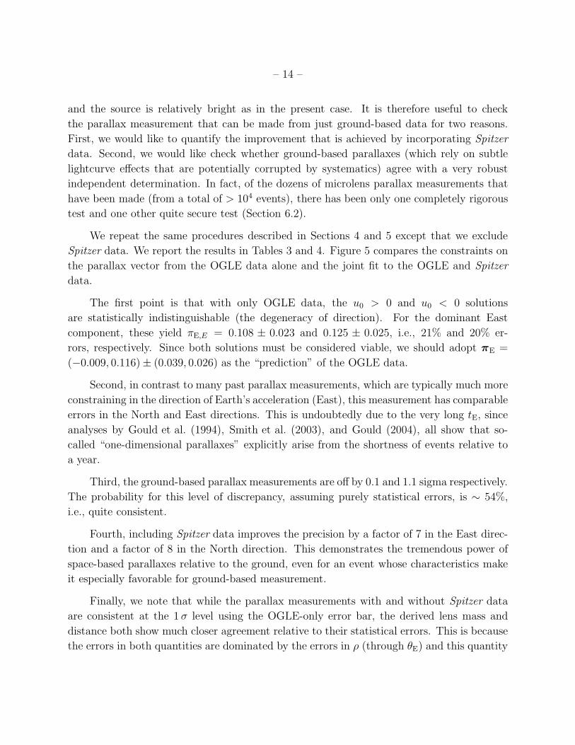
We repeat the same procedures described in Sections 4 and 5 except that we exclude
Spitzer data. We report the results in Tables 3 and 4. Figure 5 compares the constraints on
the parallax vector from the OGLE data alone and the joint fit to the OGLE and Spitzer
data.
The first point is that with only OGLE data, the u0 > 0 and u0 < 0 solutions
are statistically indistinguishable (the degeneracy of direction). For the dominant East
component, these yield πE,E = 0.108 ± 0.023 and 0.125 ± 0.025, i.e., 21% and 20% er-
rors, respectively. Since both solutions must be considered viable, we should adopt πE =
(−0.009, 0.116) ± (0.039, 0.026) as the “prediction” of the OGLE data.
Second, in contrast to many past parallax measurements, which are typically much more
constraining in the direction of Earth’s acceleration (East), this measurement has comparable
errors in the North and East directions. This is undoubtedly due to the very long tE, since
analyses by Gould et al. (1994), Smith et al. (2003), and Gould (2004), all show that so-
called “one-dimensional parallaxes” explicitly arise from the shortness of events relative to
a year.
Third, the ground-based parallax measurements are off by 0.1 and 1.1 sigma respectively.
The probability for this level of discrepancy, assuming purely statistical errors, is ∼ 54%,
i.e., quite consistent.
Fourth, including Spitzer data improves the precision by a factor of 7 in the East direc-
tion and a factor of 8 in the North direction. This demonstrates the tremendous power of
space-based parallaxes relative to the ground, even for an event whose characteristics make
it especially favorable for ground-based measurement.
Finally, we note that while the parallax measurements with and without Spitzer data
are consistent at the 1 σ level using the OGLE-only error bar, the derived lens mass and
distance both show much closer agreement relative to their statistical errors. This is because
the errors in both quantities are dominated by the errors in ρ (through θE) and this quantity
– 15 –
is poorly determined in the present case.
6.2. A Second Direct Test: MACHO-LMC-5
Spitzer observations of OGLE-2014-BLG-0124 provide only the second direct test of a
microlens parallax measurement derived from so-called “orbital parallax”, i.e., distortions
in the lightcurve due to the accelerated motion of Earth. Such tests are quite important
because microlens parallaxes are derived from very subtle deviations in the lightcurve, which
could potentially be corrupted by – or be even entirely caused by – instrumental systematics
and/or real physical processes unrelated to Earth’s motion.
In the present case, we found that the accuracy of the ground based measurement of
“orbital parallax” (as judged by the comparison to the much more precise Earth-Spitzer mea-
surement) was nearly as good as the relatively small formal errors of σ(πE) = (0.039, 0.026).
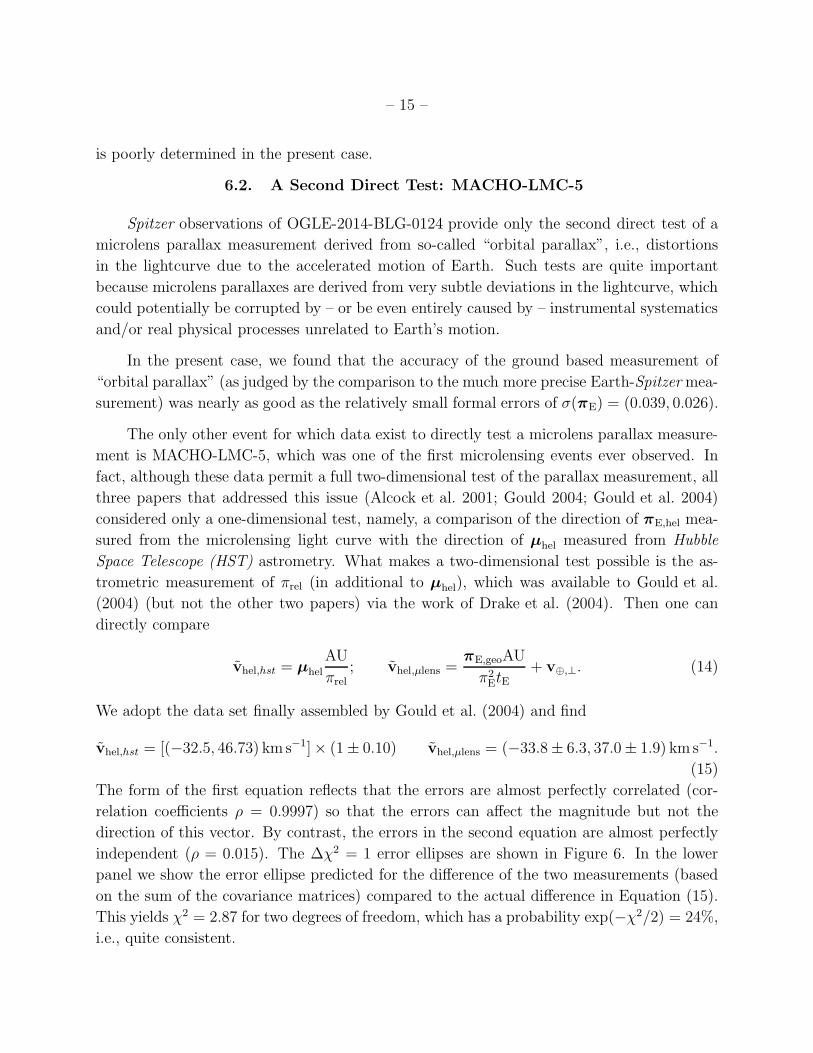
The only other event for which data exist to directly test a microlens parallax measure-
ment is MACHO-LMC-5, which was one of the first microlensing events ever observed. In
fact, although these data permit a full two-dimensional test of the parallax measurement, all
three papers that addressed this issue (Alcock et al. 2001; Gould 2004; Gould et al. 2004)
considered only a one-dimensional test, namely, a comparison of the direction of πE,hel mea-
sured from the microlensing light curve with the direction of µhel measured from Hubble
Space Telescope (HST) astrometry. What makes a two-dimensional test possible is the as-
trometric measurement of πrel (in additional to µhel), which was available to Gould et al.
(2004) (but not the other two papers) via the work of Drake et al. (2004). Then one can
directly compare
vhel,hst = µhel
AU
πrel
; vhel,µlens =πE,geoAU
π2EtE
+ v⊕,⊥. (14)
We adopt the data set finally assembled by Gould et al. (2004) and find
vhel,hst = [(−32.5, 46.73) km s−1] × (1 ± 0.10) vhel,µlens = (−33.8 ± 6.3, 37.0 ± 1.9) km s−1.
(15)
The form of the first equation reflects that the errors are almost perfectly correlated (cor-
relation coefficients ρ = 0.9997) so that the errors can affect the magnitude but not the
direction of this vector. By contrast, the errors in the second equation are almost perfectly
independent (ρ = 0.015). The ∆χ2 = 1 error ellipses are shown in Figure 6. In the lower
panel we show the error ellipse predicted for the difference of the two measurements (based
on the sum of the covariance matrices) compared to the actual difference in Equation (15).
This yields χ2 = 2.87 for two degrees of freedom, which has a probability exp(−χ2/2) = 24%,
i.e., quite consistent.

– 16 –
In addition to this direct test, there is one previous indirect test. For the case of the two-
planet system OGLE-2006-BLG-109Lb,c, the mass and distance derived from a combination
of microlens parallax and finite source effects were M = θE/κπE = 0.51 ± 0.05M⊙ and
DL = 1.49 ± 0.12 kpc. (Gaudi et al. 2008; Bennett et al. 2010). These predict a dereddened
source flux of H0 = MH + 5 log(DL/10 pc) = 5.94 + 10.87 = 16.81. From high-resolution
Keck imaging, Bennett et al. (2010) found H = 17.09 ± 0.20. They estimated an extinction
of AH = 0.3±0.2. Hence, the two estimates of H differ by ∆H = 0.01±0.28, not accounting
for intrinsic dispersion in H as a function of mass.
7. Discussion
The projected velocity v is both the most precisely and most robustly measured physical
parameter, but it is also the most puzzling. Recall from Section 3 that vhel = (0, 105) km s−1
can be derived from direct inspection of the lightcurve, values that are confirmed and mea-
sured to a precision of 3 km s−1 by the lightcurve analysis as summarized in Table 2.
From the magnitude vhel ∼ 100 km s−1, one would conclude that the lens is most likely
at intermediate distance in the disk. This is because
µ =v
AUπrel. (16)
Hence, for stars within 1–2 kpc of the Sun (so πrel ∼ πl), we have vhel ∼ v⊥,rel, i.e., the
transverse velocity of the star in the frame of the Sun. Since very few stars are moving at
∼ 100 km s−1, it is unlikely that a nearby star would have vhel ∼ 100 km s−1. By the same
token, bulge lenses have πrel . 0.03, meaning that this projected velocity measurement would
correspond to µgeo . 0.5 mas yr−1. Since typical values for bulge lenses are µgeo ∼ 4 mas yr−1
and since the probability of slow lenses scales ∝ µ2geo, bulge lenses with this projected velocity
are also unlikely. Hence, the estimate Dl = 4.1 ± 0.6 kpc from Table 2 seems at first sight
quite consistent with these general arguments.
The problem is that the direction of vhel, almost due East, is quite unexpected for disk
lenses at intermediate distance. The fact that the Sun and the lens both partake of the
Galaxy’s flat rotation curve, while the bulge sources have roughly isotropic proper motions
implies that the mean heliocentric relative proper motion should be 〈µhel〉 = µSgrA∗ =
(5.5, 3.2) mas yr−1. Hence, for an assumed distance of Dl = 4.1 kpc (πrel = 0.12 mas), there
is an offset
∆µhel = µhel − 〈µhel〉 = (−5.6, 0.5) mas yr−1. (17)
While it is not impossible that the source star is responsible for this motion (although
it is relatively large considering that the 1-dimensional dispersion of bulge lenses is σµ ∼

– 17 –
3 mas yr−1) or that there is some contribution from the peculiar motion of the lens itself,
the problem is that this unusually large motion just happens to be of just the right size
and direction to push vN ∼ 0. Of course, the lens must be going in some direction, but
East is a very special direction in the problem because that is the projected direction of the
Earth-Spitzer axis.
One generic way to produce a spurious alignment between the inferred direction of lens
motion and the Earth-Spitzer axis is to introduce “noise” in the sparse epochs of the early
Spitzer lightcurve. We do not expect instrumental noise at this level and do not see any
evidence of it in the late Spitzer light curve. However, one way to introduce astrophysical
“noise” would be to assume that the true direction of motion was very different and that
the planetary deviation seen in the Spitzer lightcurve was from a second unrelated planet.
This would require some fine-tuning because fitting even 4-5 deviated points to an already-
determined lens geometry is not trivial. However, there is a stronger argument against this
scenario: the ground-based data by themselves predict the same general trajectory (albeit
with seven times larger errors), so that even without having seen the Spitzer data, one would
predict that Spitzer would see deviations due to the ground-observed planet at approximately
this epoch.
Hence, we conclude that while the alignment of vhel with the Earth-Spitzer axis is
indeed a puzzling coincidence, there are no candidate explanations for this other than chance
alignment.
8. Conclusions
OGLE-2014-BLG-0124 is the first planetary microlensing event with a space-based mea-
surement of the vector microlens parallax πE. Combining πE and θE provides a means to pre-
cisely measure masses of the host star and planet in microlensing events. In most planetary
microlensing events, πE is the limiting factor in obtaining a direct measurement of the planet’s
mass (but see Zhu et al. 2014). In this case, the combination of data from both OGLE and
Spitzer gives an error in the amplitude of the parallax that is only 2.5%, implying that it
contributes negligibly to the uncertainty in the host mass M = θE/κπE = 0.71 ± 0.22M⊙.
Rather, in contrast to the great majority of planetary microlensing events discovered to date,
this uncertainty is dominated by the error in θE. That is, whereas most current planetary
events have caustic crossings that yield a precise measurement of ρ = θ∗/θE, so that the
fractional error in θE is just that of θ∗ (typically ∼ 7%), OGLE-2014-BLG-0124 did not
undergo caustic crossings. Rather, there is an upper limit on ρ because if it were too big, the
source would have approached close enough to a cusp to give rise to detectable effects, and a

– 18 –
lower limit because small ρ implies large θE = θ∗/ρ and thus large mass and large lens-source
relative parallax πrel = θEπE. The combination would make the lens bright enough to be seen
for ρ < 6.5 × 10⁻⁴. Hence the mass of the planet is m = 0.51 ± 0.16Mjup and its projected
separation is a⊥ = 3.1 ± 0.5 AU. It lies at a distance DL = 4.1 ± 0.6 kpc from the Sun.
The high precision of the Earth-Spitzer microlens parallax allows the first rigorous test of
a ground-based πE measurement from OGLE-only data, which yielded a 22% measurement
of πE. The Spitzer data show that this measurement is correct to within 1.1 σ. We use
archival data to construct a second test using purely astrometric HST data to confirm the
two-dimensional vector projected velocity v for MACHO-LMC-5 that was derived from the
microlensing data. These tests show that ground-based microlensing parallaxes are reliable
within their stated errors in the relatively rare cases that they can be measured.
The OGLE project has received funding from the European Research Council under
the European Community’s Seventh Framework Programme (FP7/2007-2013) / ERC grant
agreement no. 246678 to AU. Work by JCY was performed under contract with the Cali-
fornia Institute of Technology (Caltech)/Jet Propulsion Laboratory (JPL) funded by NASA
through the Sagan Fellowship Program executed by the NASA Exoplanet Science Institute.
AG was supported by NSF grant AST 1103471 and NASA grant NNX12AB99G. Work by
CH was supported by the Creative Research Initiative Program (2009-0081561) of the Na-
tional Research Foundation of Korea. This work is based in part on observations made with
the Spitzer Space Telescope, which is operated by the Jet Propulsion Laboratory, California
Institute of Technology under a contract with NASA.
REFERENCES
Alcock, C., Allsman, R.A., Alves, D.R. et al. 2001, Nature, 414, 617
Bennett, D.P., Rhie, S.H., Nikolaev, S. et al. 2010, ApJ, 713, 837
Bensby, T. Yee, J.C., Feltzing, S. et al. 2013, A&A, 549A, 147
Bessell, M.S., & Brett, J.M. 1988, PASP, 100, 1134
Claret, A. 2000, A&A, 363, 1081
Drake, A.J., Cook, K.H., & Keller, S.C. 2004, ApJ, 607, L29
Dong, S., Udalski, A., Gould, A., et al. 2007, ApJ, 664, 862

– 19 –
Dong, S., Gould, A., Udalski, A., et al. 2009, ApJ, 695, 970
Gaudi, B.S. 2012 ARA&A, 50, 411
Gaudi, B.S., Bennett, D.P., Udalski, A. et al. 2008, Science, 319, 927
Gould, A. 1994, ApJ, 421, L71
Gould, A. 1999, ApJ, 514, 869
Gould, A. 2000, ApJ, 535, 928
Gould, A. 2008, ApJ, 681, 1593
Gould, A. 2004, ApJ, 606, 319
Gould, A, Bennett, D.P., & Alves, D.R. 2004, ApJ, 614, 404
Gould, A. & Gaucherel, C. 1997, ApJ, 477, 580
Gould, A. & Horne, K. 2013, ApJ, 779, 28
Gould, A. & Loeb, A. 1992, ApJ, 396, 104
Gould, A., Miralda-Escude, J. & Bahcall, J.N. 1994, ApJ, 423, L105
Han, C. 2006, ApJ, 638,1080
Kervella, P., Thevenin, F., Di Folco, E., & Segransan, D. 2004, A&A, 426, 297
Nataf, D.M., Gould, A., Fouque, P. et al. 2013, ApJ, 769, 88
Pejcha, O., & Heyrovsky, D. 2009, ApJ, 690, 1772
Refsdal, S. 1966, MNRAS, 134, 315
Poleski, R., Udalski, A., Dong, S. et al. 2014, ApJ, 782, 47
Schechter, P.L., Mateo, M., & Saha, A. 1993, PASP, 105, 1342
Skowron, J., Udalski, A., Gould, A. et al. 2011, ApJ, 738, 87
Smith, M., Mao, S., & Paczynski, B. 2003, MNRAS 339, 925
Udalski, A. 2003, Acta Astron., 53, 291

– 20 –
Udalski, A., Szymanski, M., Kaluzny, J., Kubiak, M., Mateo, M., Krzeminski, W., & Paczyn-
ski, B. 1994, Acta Astron., 44, 317
Yee, J.C., Svartzvald, Y., Gal-Yam, A. et al. 2012, ApJ, 755, 102
Yoo, J., DePoy, D.L., Gal-Yam, A. et al. 2004, ApJ, 603, 139
Zhu, W., Gould, A., Penny, M., Mao, S., & Gendron, R. 2014, ApJ, 794, 53
This preprint was prepared with the AAS LATEX macros v5.2.

– 21 –
Table 1: µlens Parameters (Spitzer+OGLE)
Parameter Unit u0 > 0 u0 < 0
χ2/dof 6664 6671
/ 6769 / 6769
t0 − 6800 day 36.176 36.140
0.039 0.040
u0 0.1749 -0.1778
0.0039 0.0032
tE day 152.1 151.8
2.9 2.4
s 0.9443 0.9429
0.0030 0.0023
q 10−3 0.694 0.705
0.046 0.038
α deg 78.216 -78.307
0.090 0.100
ρ 10−3 1.25 1.37
0.38 0.42
πE,N -0.0055 0.0399
0.0048 0.0052
πE,E 0.1461 0.1430
0.0037 0.0037
γ‖ yr−1 -0.115 -0.119
0.017 0.016
γ⊥ yr−1 0.77 -0.97
0.53 0.45

– 22 –
Table 2: Physical Parameters (Spitzer+OGLE)
Parameter Unit u0 > 0 u0 < 0
Mhost M⊙ 0.71 0.65
0.22 0.22
Mplanet Mjup 0.51 0.47
0.16 0.15
Distance kpc 4.10 4.23
0.59 0.59
a⊥ AU 3.11 2.97
0.49 0.51
vN,hel km/s -3.0 20.6
2.6 2.9
vE,hel km/s 107.0 103.2
2.8 2.3
µhel mas/yr 2.77 2.56
0.86 0.83
β = (Ekin/Epot)⊥ 0.47 0.57
0.29 0.30
θE mas 0.84 0.78
0.26 0.25

– 23 –
Table 3: µlens Parameters (OGLE-only)
Parameter Unit u0 > 0 u0 < 0
χ2/dof 6621 6622
/ 6732 / 6732
t0 − 6800 day 36.170 36.182
0.051 0.054
u0 0.2099 -0.1964
0.0197 0.0201
tE day 131.1 140.7
9.7 13.1
s 0.9260 0.9366
0.0096 0.0097
q 10−3 0.752 0.696
0.092 0.086
α deg 78.514 -78.566
0.183 0.168
ρ 10−3 1.60 1.36
0.46 0.44
πE,N 0.0179 -0.0356
0.0122 0.0443
πE,E 0.1077 0.1251
0.0233 0.0247
γ‖ yr−1 -0.148 -0.138
0.023 0.023
γ⊥ yr−1 0.62 -0.52
0.68 0.67

– 24 –
Table 4: Physical Parameters (OGLE-only)
Parameter Unit u0 > 0 u0 < 0
Mhost M⊙ 0.81 0.74
0.20 0.21
Mplanet Mjup 0.63 0.53
0.18 0.16
Distance kpc 4.92 4.25
0.69 0.72
a⊥ AU 3.16 3.13
0.46 0.47
vN,hel km/s 28.9 -28.0
38.6 30.5
vE,hel km/s 149.6 111.5
27.5 17.2
µhel mas/yr 2.48 2.81
0.64 0.86
β = (Ekin/Epot)⊥ 0.40 0.38
0.31 0.30
θE mas 0.72 0.83
0.19 0.26

– 25 –
6807 6814
6814 6821
6821 6828
6828 6835
6835 6842
6842 6849
6849 6856
Fig. 1.— Timeline (HJD′) of Spitzer observations. Each Spitzer “week” of observations is
color-coded. The triangle indicates the date the microlensing targets were submitted to the
Spitzer Science Center for observations during the corresponding “week” indicated by the
light bands. The solid sections of the bands indicate the blocks allocated to microlensing
observations, which were taken approximately once per day. The black, vertical lines indicate
the specific observations of OGLE-2014-BLG-0124. These observations were more sparse
early in the Spitzer campaign and became more dense as the event neared peak (as seen
from Earth) and was discovered to host a planet.

– 26 –
6700 6750 6800 6850 6900HJD-2450000
−0.2
−0.1
0.0
0.1
0.2
Resi
dual (m
ag)
16.0
16.2
16.4
16.6
16.8
17.0
17.2
17.4
I (O
GLE
) [m
ag]
OGLE ISpitzer 3.6 µm
6820 6830 6840 6850
15.6
16.0
16.4
16.8
A B C D 16.1
16.2
16.3
C
+6837
0 1 2
16.2
16.3
D
+6844
Fig. 2.— Lightcurve and residuals for planetary model of OGLE-2014-BLG-0124 as observed
from Earth by OGLE in I band (black) and by Spitzer at 3.6µm (red), which was located
∼ 1 AU East of Earth in projection at the time of the observations. Simple inspection of
the OGLE lightcurve features shows that this is Jovian planet, while the fact that Spitzer
observed similar features 20 days earlier demonstrates that the lens is moving v ∼ 105 km s−1
due East projected on the plane of the sky (Section 3). Detailed model-fitting confirms and
refines this by-eye analysis (Section 5). Note that in the left inset, the Spitzer light curve is
aligned to the OGLE system (as is customary), but it is displaced by 0.2 mag in the main
diagram, for clarity.

– 27 –
"Ridges"
"Demagnified" Region
Path of
Source
Fig. 3.— Magnification map for caustic region of OGLE-2014-BLG-0124 in standard ori-
entation with planet to right. As the source passes over the “demagnified” region (darker
tones), the minor image due (to the primary lens) passes very close to the planet, which is
off the figure to the right. Because the minor image is unstable, it is easily destroyed by the
planet, which accounts for the relative demagnification. Two triangular caustic regions flank
the deepest part of this demagnification. The source does not cross these causitics, but does
cross the two ridges that extend from the cusps, toward the left. It is these ridges that are
responsible for the two bumps near t = 6820 and t = 6825 (from Spitzer) or t = 6839 and
t = 6845 (from Earth) in Figure 2.

– 28 –
0.1 0.0 -0.1 -0.2θ/θE (East)
−0.1
0.0
0.1
0.2
θ/θ E
(N
ort
h)
Earth
Spitzer
A: 6820.6B: 6825.1C: 6838.6D: 6844.8
A B C D
u0,+ solution
0.5 0.0 -0.5−1.0
−0.5
0.0
0.1 0.0 -0.1 -0.2θ/θE (East)
−0.2
−0.1
0.0
0.1
θ/θ E
(N
ort
h)
Earth
Spitzer
A: 6820.6B: 6825.1C: 6838.6D: 6844.8
A BC D
u0,− solution
0.5 0.0 -0.5
0.0
0.5
1.0
Fig. 4.— Lens geometry for OGLE-2014-BLG-0124. North is up and East is left. The lens
position is fixed, but with its orientation rotating at dα/dt and the planet-star separation
changing by ds/dt, with the four epochs at which the source passes the two caustic “prongs”
as seen from Spitzer and Earth shown in different colors. The source positions as seen from
OGLE (black) and Spitzer (red) are shown for each epoch of observation. These trajectories
deviate slightly from rectilinear motion because of parallax effects of each observatory’s
motion. The line segments indicate common times at the two observatories, which illustrate
that the Earth-Spitzer projected separation increases substantially over the 35 days of Spitzer
observations. The left (right) panel shows the geometry of the u0 > 0 (u0 < 0) solutions,
which are very similar except for orientation (see Tables 1 and 2). Planet location is indicated
by “+” symbols in insets.

– 29 –
πE,E
π E,N
.2 .15 .1 .05 0
−.1
−.05
0
.05
.1
OGLE (+)
OGLE (−)
SPITZER+OGLE (−)
SPITZER+OGLE (+)
Fig. 5.— Error contours (∆χ2 = 1) in the πE plane for two solutions (u0 > 0 and u0 < 0)
for each of two cases (OGLE-only and Spitzer+OGLE), shown in standard and bold curves,
respectively. For Spitzer+OGLE, the u0 < 0 solution is displayed as a dashed curve as a
reminder that this solution is disfavored but not formally excluded (∆χ2 = 7). By contrast,
the OGLE-only solutions differ by ∆χ2 = 1. The u0 > 0 and u0 < solutions are indicated
by (+) and (-), respectively.

– 30 –
vhel,E (km/s)
v hel,N
(km
/s)
55 50 45 40 35 30
−35
−30
−25
−20MACHO−LMC−5 Test
HST
Astrometry Ground
µlensing
∆vhel,E (km/s)
∆vhe
l,N (
km/s
)
15 10 5 0 −5 −10−5
0
5
10 Difference
ObservedPredicted
Fig. 6.— Upper Panel: Comparison of projected velocity v as determined from microlensing
lightcurve and HST astrometry for MACHO-LMC-5, which was discovered by the MACHO
group in 1993. Lower Panel: Predicted difference (zero with error ellipse) between these two
measurements compared to observed difference. The ∆χ2 = 2.87 (for 2 dof) implies con-
sistency at the 24% level. MACHO-LMC-5 is the only ground-based parallax measurement
(other than OGLE-2014-BLG-0124) for which such a rigorous test is possible. Both events
pass this test.