Spectrum Measurements with SmaartLive: Concepts and ... · Spectrum-Mode Measurements with...

Spectrum-Mode Measurements with SmaartLive: Concepts and Applications

Spectrum Measurements with SmaartLive: Concepts and Applications

Paul D. Henderson

A key component of the SmaartLive application is its Spectrum mode, which provides a highly flexible FFT-based real-time analyzer capable of advanced audio signal measurements. The spectrum mode is useful in many applications, including noise and sound exposure measurements, the location of feedback frequencies in sound reinforcement, and cinema system optimization, as well as general signal monitoring tasks. This document serves as an introduction to effectively applying the Spectrum mode measurement capabilities. A general knowledge of the topics covered in “Getting Started with SmaartLive” and “The Fundamentals of FFT-Based Audio Measurements in SmaartLive” will be helpful when reading this text. I. Basic Spectrum Analysis The real-time analyzer, or RTA, is a familiar tool to audio professionals, allowing the user to view the spectral content of audio signals throughout a system. Traditionally, RTAs were constructed as dedicated hardware devices, capable of displaying signal power versus frequency in fractional-octave bands. In early devices, banks of analog filters separated the spectrum into constant-percentage bandwidth sub-bands, and a level detector circuit was used to drive the unit’s display. The result was a limited-resolution frequency domain view of the spectrum of the incoming signal (Figure 1), akin to the limited-time view provided by an oscilloscope.

Frequency

Ampl

itude

Figure 1: Traditional real-time analysis: fixed & limited resolution.

SmaartLive provides an advanced alternative to traditional RTAs, taking advantage of the computational efficiency afforded by the Fast Fourier Transform (FFT) and digital signal processing. SmaartLive has the capability to provide a much higher spectral resolution than filter-based approaches, and can simultaneously acquire a temporal signature of spectral changes over time. SmaartLive can display the fine structure of the linear-frequency FFT spectrum of the input signal or may be configured to show a fractional-octave (banded) view with similar response to a hardware RTA. This section will introduce the various measurement techniques used throughout the Spectrum mode, specifically targeting those measurement tasks that do not require an absolute-level calibration. Several applications are reviewed, including monitoring and troubleshooting of audio equipment and the location of electroacoustical feedback frequencies.


Figure 3: Default live RTA spectrum display (1/12th-octave). Green curve: microphone, blue curve: mixer output.

Monitoring Audio Signals For this application, we will investigate the use of the Spectrum mode to view the frequency content of generic audio signals, such as those received by a microphone or output by a mixing console. Figure 2 shows a simple measurement configuration for this task, where SmaartLive monitors the output of both a microphone preamplifier and a mixing console. While a simple configuration, the connection diagram in Figure 2 is a powerful tool for use in sound reinforcement, as SmaartLive may be instantly switched between the Spectrum and Transfer Function modes for quick access to information for both equalization purposes (the transfer function) and the live signal spectrum.

MeasurementMicrophone

MicrophonePreamplifier

Computer with SmaartLiveTM

LineInput

L

R

Mixing Console

Figure 2: Monitoring microphone and mixing console signals. Basic RTA Use If we launch SmaartLive with its default parameters and start the Spectrum mode, we will see a graph representing the signal power-versus-frequency in 1/12th-octave frequency bands for both input channels (see Figure 3). You will note that the time response of the RTA display is quite fast; this is due to the short time constant (186 ms) and the fact that there is no frame averaging applied to the display (averages = 1). A fast time response is useful only for very specific applications, primarily when a joint time-frequency analysis of a signal is desired, such as with a spectrograph (as we will see later). This short time constant also provides minimal low-frequency resolution, where the frequency resolution

in this case is 5.4 Hz. As you can see in Figure 3, the low-frequency bands seem to have a smooth appearance, due to the low density of FFT data bins at these low frequencies. To improve the spectral view, we can increase the FFT size and use frame averaging to adjust the time response of the display. Changing the FFT size to 16k-bins and the averaging to slow

üTechnical Note

The exponential averaging modes in SmaartLive conform to the ANSI S1.4-1983 standard, where the exponential time constants t are as follows:

Fast: t = 125 ms Slow: t = 1000 ms


Set activetrace

Show/hidetraces

provides both additional low-frequency resolution and a more stabilized time response. The slow characteristic is based on a running exponential integration, and is useful for continuous signal monitoring during a live performance, noise level measurements, etc. The fast characteristic provides a much more immediate time response, and is useful for viewing transient signal information, such as specific musical notes. Note that the spectrum mode also allows for FIFO-style frame averaging, but, in most cases, this averaging technique is seldom required or recommended for Spectrum mode measurements. Note that both banded (1/24th, 1/12th, 1/6th, 1/3rd, and 1/1-octave) and narrowband (linear- and log-spaced) views are available. For a more detailed treatment of the FFT, averaging, and banding parameters, please see the article “The Fundamentals of FFT-Based Audio Measurements in SmaartLive”. You will note that, by default, the Spectrum display shows two separate traces, one for each input channel. SmaartLive contains a set of simple controls for managing the display of the two input channels, located directly underneath the input signal level meters. You may define either of the two input channels as the active channel by clicking the active indicators below the level meter. The current active trace will be brought to the front of the spectrum display, and the SPL Meter, SPL History Graph and Spectrograph displays will reflect the input signal from this channel only. The color of each of these displays will change to reflect the currently active channel. When using these advanced functions, it is important to note that the appropriate input channel is selected as active in order to obtain valid data. In addition, clicking the show/hide channel buttons will enable or disable the display of the associated spectrum in the RTA window. By default, traces in the RTA view contain peak hold bars, which hold the maximum value of the measurement parameter at each band or bin for a specified period of time. The configuration parameters for the peak hold mode may be found in the Input Options dialog box, which may be launched with the menu command Options? Input, or by pressing the key combination Alt+I. The hold time can be customized or an infinite hold mode may be activated, which holds the detected peak levels for an indefinite period of time until the next buffer reseed (performed by pressing the V key on the keyboard). In addition, the peak hold bars may be removed from the display for a more continuous, orderly appearance.

By hovering the mouse pointer over the RTA spectrum, the level and center frequency of the selected band is shown in the readout above

the trace display. In addition to this function, SmaartLive can display the musical note associated with the band center frequency using Note ID mode. Note ID mode may be toggled using the View? Note ID menu item. In addition, a reference piano keyboard may be activated using the Graph Options dialog box, accessible under menu item Options? Graph. You may use SmaartLive’s reference trace functions to save a snapshot of the measured spectrum to a storage register for later recall and on-screen comparison. SmaartLive contains five reference registers (A, B, C, D & E), each capable of storing up to four individual traces. As an example,

clicking the button for register A1 (the first register button in the A group) will activate this memory location. Click the button below the plot area to sample and display the current trace as an overlay on the plot. Note that the curve that will be captured is the current active trace, as defined above. The reference register stores the raw, post-


Figure 4: 1/3rd octave long-term spectrum of a musical performance.

averaging FFT data, so the curve may be later viewed using any desired fractional-octave banding or narrowband display scheme. Viewing a Long-Term Spectrum Average The averaging buffer may be set to Inf, which will provide an equal-time-weighted average of the entire signal spectrum since the last buffer reseed. This method can provide you with a view of the long-term spectrum of the signal, a measure of the “spectral signature” of the input signal. For example, the 1/3rd-octave spectrum in Figure 4 is a long-term average of a musical performance. This technique is also useful for capturing a stable measure of the continuous noise level in a room, which will be discussed later. Note that pressing the V key on the keyboard will reseed the averaging buffer, restarting the infinite averaging procedure at any desired time. Performing Harmonic Distortion Estimates An interesting and sometimes-overlooked feature of SmaartLive’s Spectrum mode is its capability to perform a rough Total Harmonic Distortion or THD measurement at a single frequency. THD is a metric used to quantify the nonlinear distortion of a system or device. A system with nonlinear distortion will output multiple frequencies for a single-frequency (sinusoidal) input, where those output frequencies will be multiples (or harmonics) of the input signal. This is typically due to a nonlinear “transfer characteristic” between the system input and output, which can be caused by tape saturation, digital clipping, transistor saturation, or nonlinear effects in loudspeakers. SmaartLive’s THD capability is useful for quantifying the distortion measure of analog recording devices and power amplifiers, as well as for determining a (rough) distortion metric for loudspeakers. For this measurement, you will need to use SmaartLive’s internal generator to output a single-frequency tone into the device-under-test at a reference frequency, and a low-distortion audio interface. The measured THD will represent the total distortion of the entire measurement system, so it is imperative that the measurement system have significantly lower distortion than the device under test. Figure 5 shows an example configuration, where a THD measurement of a loudspeaker is being performed. By placing the RTA in 1/24th-octave resolution mode and activating the menu item under View? Cursor? Show THD, SmaartLive will calculate the total harmonic distortion from the amplitude of the fundamental and subsequent harmonics at the current cursor

Figure 5: Sample THD measurement of a small loudspeaker at 200Hz: THD=0.12%.


position. Set the generator to Sine Wave to output a single frequency of choice, and place the cursor at that frequency. It may be necessary to increase the FFT size to maximize the low-frequency resolution of the measurement. Figure 5 shows a sample measurement of a small loudspeaker at 200Hz. For the measurement of a loudspeaker, the room should be very quiet, and a low-distortion microphone should be employed. Note that you may also use the Show Harmonics feature of SmaartLive by pressing Ctrl+H, which will activate a grid marking the harmonics relative to the locked cursor position. See the SmaartLive User Guide for more information. II. Viewing Spectral Changes in Time: the Spectrograph Many audio signals that are encountered in the field are highly dynamic: musical signals, speech, and even environmental noise contain significant changes in spectral content as a function of time. While the classical RTA spectrum display is useful for viewing the time-averaged spectral content of a signal, a display technique is required to enable the analysis of the incoming spectrum over time. SmaartLive’s Spectrograph mode fulfills this requirement, providing a three-dimensional view of the incoming signal: energy versus frequency versus time (Figure 6). The spectrograph can be thought of as a record of multiple RTA spectrums taken over time, with color representing amplitude. Using this functionality, the spectral content of the input signal is recorded as it changes in time, allowing the user to view and analyze time-varying trends in the input signal. The Spectrograph display is launched while in Spectrum mode by pressing the button. Note that the Spectrograph display is derived from the current active trace.

Figure 6: An example spectrograph of a musical performance. As a troubleshooting tool, the Spectrograph mode is useful for finding spectral “defects” in a system or acoustical environment. Certain audio signals or acoustical events contain specific traits that can be easily detected due to their distinct time/frequency signature, specifically, highly tonal sounds such as AC line noise in an electrical signal chain or the presence of electroacoustical feedback. Configuring the Spectrograph In order to achieve optimal results with this measurement mode, the Spectrograph configuration options must be properly set up for the measurement task at hand. The input banding, color range, and time averaging options are critical to achieving readable displays with this mode. The Spectrograph Options dialog may be launched using menu item Options? Spectrograph or by clicking the Spectro Range scale indicator. This dialog allows you to configure the color scale and amplitude range as well as the frequency and time axis


behavior. When configuring the spectrograph, the following issues are important to note:

• Spectrum banding: The banding scale of the spectrograph display tracks the selected banding of the RTA. For most applications, a 1/24th-octave or log-narrowband scale provides the best broadband frequency resolution. Low fractional-octave resolutions typically result in a rough appearance.

• Time response: By default, the time response of the spectrograph display tracks the averaging depth selected for the RTA. However, excessive averaging (or averaging at all) can obscure time-based details in the spectrograph, such as in Figure 7b. For most applications, check the Instantaneous Spectrograph box in the Spectrograph Options dialog. With this option, each spectrograph frame will represent a minimum-width time slice of the input signal, improving the time response of the display (Figure 7a). In addition, the number of FFT frames contained within the spectrograph may be set in the Frames to show in Spectrograph field. Higher numbers yield a slower time response, with more time history contained within the window. Conversely, lower numbers produce faster movement along the time axis. The absolute-time length of the time axis is a function of this value and the speed of your computing hardware.

• Amplitude range: It is imperative that an appropriate amplitude range be selected in order to reveal the desired amplitude details from the input signal. The current range is configured using the Min dB and Max dB boxes in the options dialog. Selecting too large an amplitude range may obscure amplitude details by plotting a minimal change in color as the input spectrum changes (Figure 7c), and too narrow a range or values too high or low may lead to undershoot and overshoot errors (Figure 7d). The selection of an appropriate scale will enable the detection of spectral details with high definition in amplitude, as in Figure 7a.

See the SmaartLive User’s Guide for information regarding additional configuration options for the spectrograph display.

(a): Instantaneous spectrograph, acceptable magnitude

range calibration & good time resolution (b): Slow-weighted time response,

time-domain details lost

(c): Magnitude range too wide,

amplitude details lost (d): Signal exceeds maximum magnitude range limit,

peaks lost in clipping (white regions)

Figure 7: The effect of selecting various spectrograph parameters; 1/24-octave banded spectrograph of an identical input signal.


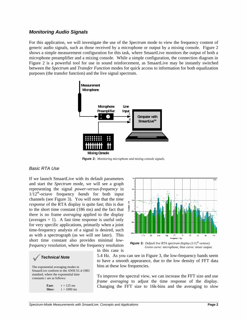
Locating Feedback Frequencies in Sound Reinforcement Here, we will discuss the use of SmaartLive in determining electroacoustic feedback frequencies in sound reinforcement and/or stage monitoring systems. The location of feedback frequencies during live sound performance is a task especially well-suited for the Spectrograph mode, which provides an advantage to detecting the unique time/frequency signature of feedback ring tones.


LineInput

L

R

Mixing Console

PowerPreamplifierEqualizer

Stage MonitorMicrophone

Acoustical Environment

Figure 8: Finding feedback frequencies in a stage monitoring system.

Figure 8 shows a simplified stage monitoring system with SmaartLive configured to monitor the console output signal before the equalizer. On a practical note, this connection can be made on the console’s wedge output with access to the solo bus, so that any monitor output send can be retrieved immediately. A typical optimization process for a stage monitor system would entail an accurate equalization process using SmaartLive’s Transfer Function mode, followed by in-show dynamic equalizer changes based on feedback modes that may be found as the acoustical environment varies. Note that a feedback mode in an electroacoustical system needs two components to begin “ringing” (or regenerating): a system-borne instability at any frequency and ambient sound energy at that frequency to initiate the regeneration. Therefore, it is imperative to note that using any method to locate feedback frequencies (commonly known as “ringing out” a system) without active signals in the system (such as a live performance) will result in inaccurate adjustments. If this process is performed without ambient sound such as in a pre-show configuration, some broadband energy should be introduced to the system (such as low-level pink noise). Electroacoustical feedback is created by narrowband loop-path instability, and is primarily a single-frequency effect, although multiple feedback modes may be excited simultaneously.


Feedback Signature

Figure 9: Feedback signatures in spectrograph and spectrum displays.

This time-domain element of the spectrograph can be exploited in the task of finding feedback frequencies, since the ringing of electroacoustical feedback has a time-domain signature, i.e., it is constant in frequency and has both a duration and envelope in time. Narrowband constant-frequency signals such as a feedback ring tone or tonal noise source show up as horizontal lines in the spectrograph, making it somewhat easier to find these effects in the presence of a more complex signal, such as a live musical performance. Figure 9 illustrates this effect, as well as the simultaneous use of the spectrograph and RTA displays. An additional advantage of this technique is that the operator can immediately reduce the gain to eliminate the feedback loop on the console, and the running spectrograph will contain a history of the ring frequency for subsequent equalization changes. Note that, when controlling compatible external signal processors, their control parameters may be changed without leaving Spectrum mode. A Control frequency response display will appear, allowing you to view calculated EQ traces for compatible devices just as in the Transfer Function mode. III. Performing Calibrated Measurements For the measurement procedures introduced in Section I, SmaartLive was in its uncalibrated state: the values displayed were relative to the maximum full-scale range of the analog-to-digital converter. However, some measurement procedures require absolute calibration, where the displayed values are calibrated relative to real-world physical quantities. While SmaartLive can be calibrated to any decibel-based scale (dBu, dBm, etc.), the most commonly-used absolute scale is dB-SPL.


Calibrating the System for SPL Measurement

MeasurementMicrophone

MicrophonePreamplifier


LineInput

L

R

Calibrator

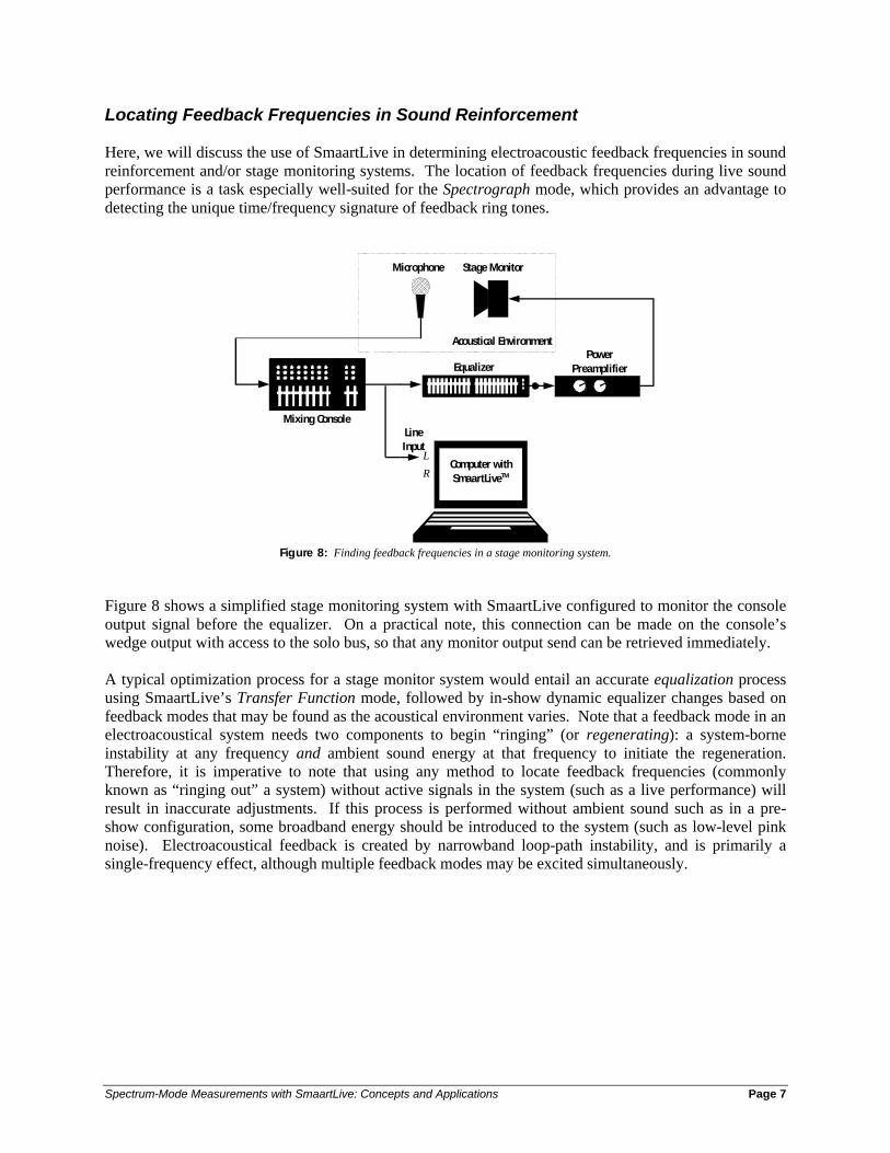
Figure 10: The SPL calibration process.

In Spectrum mode, the entire system can be calibrated in a single step, including the built-in sound level meter. Several techniques are outlined in the User Guide for performing the calibration, but we will cover only the most accurate and widely-accepted procedure, which utilizes a sound level calibrator as an absolute level reference (see Figure 10). The calibrator should be correctly sized for your measurement microphone in order to ensure an airtight seal with the capsule. Most calibrators output a 1 kHz reference tone at one of the following reference levels: 94, 104, or 114 dB-SPL. Choose an appropriate reference level and adjust your microphone preamplifier gain to achieve sufficient headroom with this

reference pressure. Place SmaartLive into 1/3rd-octave RTA mode. The 1/3rd octave mode is employed to make certain that all of the energy from the windowed sinusoid is taken into account. If calibration is performed in a narrowband or high-resolution mode, the time window effects may distribute a significant portion of the sinusoid energy into surrounding bands. Select the input channel from the microphone as the active channel. Next, double-click on the 1 kHz band (or other band if your calibrator uses a different center frequency), and the Amplitude Calibration dialog will open. Select “Set this value to...” and enter the level of your calibrator. The system is now calibrated to Sound Pressure Level for the current

channel only, unless a microphone and preamplifier with identical sensitivity and gain are connected to the opposite channel. Note that any change in the preamplifier or sound card gain will necessitate recalibration. If the clip indicators in SmaartLive illuminate during use, reduce the preamplifier gain and recalibrate for additional headroom. Measuring Sound Pressure Level

Now that the system is calibrated to SPL, we can perform accurate sound level measurements in any environment. You will note that the digital readout above the input level meters now displays dB-SPL with a Fast integration time. By clicking on the readout, you will be taken to the SPL Readout Options dialog, which enables you to configure the SPL meter component with various weighting curves and integration speeds, as well as configuration options for peak hold, SPL alarms, and logging capabilities. The peak hold and alarm functions are quite useful for live

sound and noise level monitoring tasks, helping to maintain compliance with noise ordinances and safety regulations. The following sections will discuss the available weighting curves and integration speeds and their appropriate uses.

üTechnical Note

0 dB-SPL = 20 µPa RMS 94 dB-SPL = 1 Pa RMS 104 dB-SPL = 3.2 Pa RMS 114 dB-SPL = 10 Pa RMS


Weighting Curves For measuring sound pressure levels, SmaartLive includes three available weighting curves. A weighting curve is a filter response that is placed in-line with the SPL meter detector before the displayed value is calculated; the filter allows the response of the detector to vary as a function of frequency. SmaartLive contains Flat, A and C weighting filters, whose frequency response curves are shown below in Figure 11. The Flat weighting curve is exactly as the name implies: it has a perfectly linear response over frequency, meaning that the SPL meter will respond equally to equal acoustic pressure at any frequency inside its range. The Flat characteristic is useful for determining the total sound pressure at a point in space, as well as for sound power estimation tasks (beyond the scope of this document). The A and C weighting curves are drawn from the ANSI S1.4-1983 standard. The C weighting curve contains a slight high-frequency and low-frequency rolloff, meaning that the SPL meter detector is less sensitive to energy in those regions of the spectrum. The A weighting curve contains a much more dramatic low-frequency rolloff, indicating a primary sensitivity in the region above 1 kHz. Often, the background work that leads us to these specific curves is overlooked: the A and C curves are approximate inverses of the equal-loudness contours of human hearing at the 40 phon and 100 phon contour levels, respectively. The science behind the equal-loudness contours will not be presented here, but, suffice it to say that the A weighting curve approximates the response of human hearing at low levels, and the C weighting curve does the same at high levels. Most noise level measurement standards have taken the A weighting function as customary, as, even at high levels, it more correctly approximates both the annoyance level of the noise and the potential for hearing damage. It should be stated that the suffix dBA is commonly attached to sound pressure readings in the A weighting scale, and similarly dBC for the C weighting scale. Flat-weighted measurements are typically suffixed with dB-SPL. Integration Speeds SmaartLive contains three integration speeds for the SPL display: Inst, Slow, and Fast. The Inst setting effectively corresponds to the Impulse setting on a typical high-end sound level meter, as it displays the latest SPL data from the sound card with no averaging integration. This setting can be combined with the Peak Hold function to capture the peak sound level in an environment, specifically where there are impulsive and transient noise sources. The Fast and Slow settings are ANSI-standard exponential integration curves. The Fast setting is useful for finding standardized peak sound levels, again, best with the Peak Hold function or in conjunction with the SPL logging plot (to be discussed later). The Slow setting is perhaps the most useful for typical measurements, as it provides a longer integration time for more accurately representing the average sound level in the environment. The Slow response is also widely accepted in standards for studies in sound exposure and noise pollution (such as during a live performance).

Figure 11: SPL weighting curves.

102

103

104

-60

-50

-40

-30

-20

-10

0

10

Frequency (Hz)

Mag

nitu

de (

dB)

Flat WeightingA WeightingC Weighting


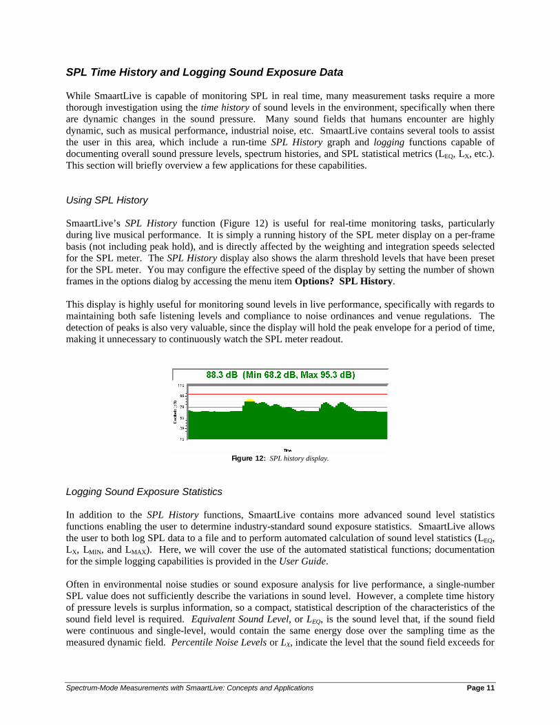
SPL Time History and Logging Sound Exposure Data While SmaartLive is capable of monitoring SPL in real time, many measurement tasks require a more thorough investigation using the time history of sound levels in the environment, specifically when there are dynamic changes in the sound pressure. Many sound fields that humans encounter are highly dynamic, such as musical performance, industrial noise, etc. SmaartLive contains several tools to assist the user in this area, which include a run-time SPL History graph and logging functions capable of documenting overall sound pressure levels, spectrum histories, and SPL statistical metrics (LEQ, LX, etc.). This section will briefly overview a few applications for these capabilities. Using SPL History SmaartLive’s SPL History function (Figure 12) is useful for real-time monitoring tasks, particularly during live musical performance. It is simply a running history of the SPL meter display on a per-frame basis (not including peak hold), and is directly affected by the weighting and integration speeds selected for the SPL meter. The SPL History display also shows the alarm threshold levels that have been preset for the SPL meter. You may configure the effective speed of the display by setting the number of shown frames in the options dialog by accessing the menu item Options? SPL History. This display is highly useful for monitoring sound levels in live performance, specifically with regards to maintaining both safe listening levels and compliance to noise ordinances and venue regulations. The detection of peaks is also very valuable, since the display will hold the peak envelope for a period of time, making it unnecessary to continuously watch the SPL meter readout.

Figure 12: SPL history display.

Logging Sound Exposure Statistics In addition to the SPL History functions, SmaartLive contains more advanced sound level statistics functions enabling the user to determine industry-standard sound exposure statistics. SmaartLive allows the user to both log SPL data to a file and to perform automated calculation of sound level statistics (LEQ, LX, LMIN, and LMAX). Here, we will cover the use of the automated statistical functions; documentation for the simple logging capabilities is provided in the User Guide. Often in environmental noise studies or sound exposure analysis for live performance, a single-number SPL value does not sufficiently describe the variations in sound level. However, a complete time history of pressure levels is surplus information, so a compact, statistical description of the characteristics of the sound field level is required. Equivalent Sound Level, or LEQ, is the sound level that, if the sound field were continuous and single-level, would contain the same energy dose over the sampling time as the measured dynamic field. Percentile Noise Levels or LX, indicate the level that the sound field exceeds for


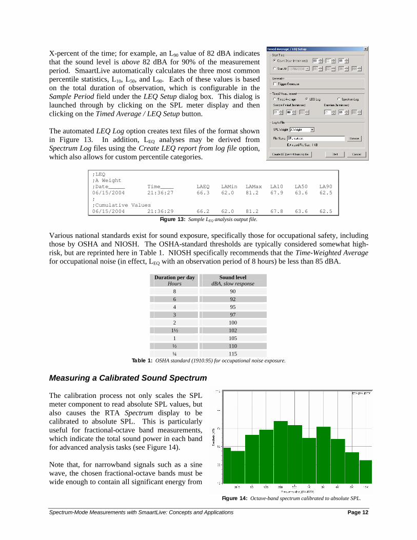
X-percent of the time; for example, an L90 value of 82 dBA indicates that the sound level is above 82 dBA for 90% of the measurement period. SmaartLive automatically calculates the three most common percentile statistics, L10, L50, and L90. Each of these values is based on the total duration of observation, which is configurable in the Sample Period field under the LEQ Setup dialog box. This dialog is launched through by clicking on the SPL meter display and then clicking on the Timed Average / LEQ Setup button. The automated LEQ Log option creates text files of the format shown in Figure 13. In addition, LEQ analyses may be derived from Spectrum Log files using the Create LEQ report from log file option, which also allows for custom percentile categories.

;LEQ ;A Weight ;Date_____ Time____ LAEQ LAMin LAMax LA10 LA50 LA90 06/15/2004 21:36:27 66.3 62.0 81.2 67.9 63.6 62.5 ; ;Cumulative Values 06/15/2004 21:36:29 66.2 62.0 81.2 67.8 63.6 62.5

Figure 13: Sample LEQ analysis output file. Various national standards exist for sound exposure, specifically those for occupational safety, including those by OSHA and NIOSH. The OSHA-standard thresholds are typically considered somewhat high-risk, but are reprinted here in Table 1. NIOSH specifically recommends that the Time-Weighted Average for occupational noise (in effect, LEQ with an observation period of 8 hours) be less than 85 dBA.

Duration per day Hours

Sound level dBA, slow response

8 90 6 92 4 95 3 97 2 100

1½ 102 1 105 ½ 110 ¼ 115

Table 1: OSHA standard (1910.95) for occupational noise exposure.

Measuring a Calibrated Sound Spectrum The calibration process not only scales the SPL meter component to read absolute SPL values, but also causes the RTA Spectrum display to be calibrated to absolute SPL. This is particularly useful for fractional-octave band measurements, which indicate the total sound power in each band for advanced analysis tasks (see Figure 14). Note that, for narrowband signals such as a sine wave, the chosen fractional-octave bands must be wide enough to contain all significant energy from

Figure 14: Octave-band spectrum calibrated to absolute SPL.


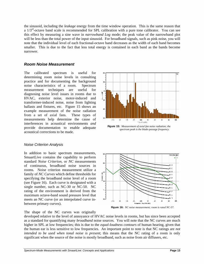
the sinusoid, including the leakage energy from the time window operation. This is the same reason that a 1/3rd-octave band scale is recommended for SPL calibration with a pure tone calibrator. You can see this effect by measuring a sine wave in narrowband Log mode; the peak value of the narrowband plot will be less than the total power of the input sinusoid. For broadband signals, such as pink noise, you will note that the individual level of each fractional-octave band decreases as the width of each band becomes smaller. This is due to the fact that less total energy is contained in each band as the bands become narrower. Room Noise Measurement The calibrated spectrum is useful for determining room noise levels in consulting practice and for documenting the background noise characteristics of a room. Spectrum measurement techniques are useful for diagnosing noise level issues in rooms due to HVAC, exterior noise, motor-induced and transformer-induced noise, noise from lighting ballasts and fixtures, etc. Figure 15 shows an example measurement of the noise radiation from a set of axial fans. These types of measurements help determine the cause of interferences in acoustical environments and provide documentation to enable adequate acoustical corrections to be made. Noise Criterion Analysis In addition to basic spectrum measurements, SmaartLive contains the capability to perform standard Noise Criterion, or NC measurements of continuous, broadband noise sources in rooms. Noise criterion measurement utilize a family of NC Curves which define thresholds for specifying the broadband noise level of a room (see Figure 16). Each curve is designated with a single number, such as NC-30 or NC-50. NC rating of the environment is derived from the maximum octave-band sound pressure level that meets an NC curve (or an interpolated curve in-between primary curves). The shape of the NC curves was originally developed relative to the level of annoyance of HVAC noise levels in rooms, but has since been accepted as a standard for quantifying many broadband noise sources. You will note that the NC curves are much higher in SPL at low frequencies; this is due to the equal-loudness contours of human hearing, given that the human ear is less sensitive to low frequencies. An important point to note is that NC ratings are not intended to be used when tonal noise is present; this means that the NC rating of a room is only significant when the source of the noise is mostly broadband, such as noise from air diffusers, etc.

Figure 15: Measurement of axial fan noise radiation; the spectrum peak is the blade-passage frequency.

Figure 16: NC noise measurement; room is rated NC-57.


Cinema System Certification An application that commonly requires an RTA for measurement is the certification of cinema and home theater systems to industry standards. While it is recommended that high-resolution equalization and loudspeaker setup tasks be performed with SmaartLive’s Transfer Function and Impulse Response modes, most cinema standards groups require an RTA-based (usually 1/3rd-octave) measurement for certification. This section will not cover the specific standards, but will review specific capabilities in SmaartLive for performing these measurements. Timed Spectral Averaging SmaartLive contains a Timed Spectral Averaging mode that allows for long-term acquisition of average spectra present in the environment. This mode is accessed by clicking on the SPL meter display and then clicking on the Timed Average / LEQ Setup button. As with LEQ measurements, you may select any observation period for the measurement. The result of this acquisition process is placed into a user-defined reference register. Because of the potential for a very long integration time, Timed Spectral Averaging is valuable for obtaining highly stable measurement results with random noise sources, such as the use of pink noise during an equalization process or for quantifying broadband room noise. Verifying Filter Calibration Typical large-format cinema systems utilize the ANSI/SMTPE 202M X-curve for equalization of the main loudspeaker system. The X-curve, shown in Figure 17, provides a uniform 3 dB/octave high frequency rolloff beyond 2 kHz, and a (somewhat less important) low-frequency 3 dB/octave rolloff below 63 Hz. When a cinema system in a large room is equalized to this specification, less high frequency energy will reach the listeners, which has been found to be more audibly-pleasing than a flat response when the listeners are seated at a distance from the loudspeaker system. When certifying these systems for cinema use, the Inverse X-curve may be activated under the Weight spinner for the RTA. Now, with pink noise excitation, a loudspeaker system correctly conforming to the X-curve will display a flat 1/3rd-octave spectrum in the RTA display.

102

103

104

-10

-5

0

5

Frequency (Hz)

Mag

nitu

de (

dB)

Figure 17: ANSI/SMTPE 202M X-curve.


Spatial Averaging In many cinema standards, spatial averaging of measured spectra is required in order to verify that the correct performance is obtained across the entire audience area. SmaartLive simplifies this task using Reference Trace Averaging, which allows several measurements to be performed at different seating positions and then power-averaged to produce an overall performance curve. In order to average up to four reference traces, capture each measurement into a separate reference bank (i.e., A1, B1, C1, and D1). The E bank is used to hold the average; activate the E register, press the button, and the press the button. The averaged curve will appear on screen with the original reference curves (Figure 18).

Figure 18: Spatial averaging of 1/3rd-octave RTA measurements using the averaging buffers.

Gray curves: individual measurements, Red curve: spatial average. Suggestions for Further Reading

D. Davis, C. Davis: Sound System Engineering, 2nd edition. Carmel, IN: SAMS. 1994. M. Mehta, J. Johnson, C. Rocafort: Architectural Acoustics: Principles and Design. Upper Saddle

River, NJ: Prentice Hall. 1999. American National Standard: Specification for Sound Level Meters, ANSI S1.4-1983. New York,

NY: Acoustical Society of America. 1983. R. Cabot, B. Hofer, R. Metzler: Standard Handbook of Video and Television Engineering: Chapter

13.3: “Nonlinear Audio Distortion”, 4th edition. McGraw-Hill Professional. 2003.

OSHA Standard: Occupational Noise Exposure, OSHA 1910.95. Washington, DC: Occupational Safety & Health Administration. 1996.

Criteria for a Recommended Standard Occupational Noise Exposure, Revised Criteria 1996,

DHHS (NIOSH) Publication No. 96. Atlanta, GA: National Institute for Occupational Safety & Health. 1996.

Motion-Pictures - B-Chain Electroacoustic Response - Dubbing Theaters, Review Rooms and

Indoor Theaters, SMPTE 202M-1998. White Plains, NY: Society of Motion Picture and Television Engineers. 1998.

Spectrum Measurements with SmaartLive: Concepts and ... · Spectrum-Mode Measurements with...

Documents

Transcript of Spectrum Measurements with SmaartLive: Concepts and ... · Spectrum-Mode Measurements with...