SPECTRAL INEQUALITIES IN QUANTITATIVE FORM
71
SPECTRAL INEQUALITIES IN QUANTITATIVE FORM LORENZO BRASCO AND GUIDO DE PHILIPPIS Abstract. We review some results about quantitative improvements of sharp inequalities for eigenvalues of the Laplacian. Contents 1. Introduction 2 1.1. The problem 2 1.2. Plan of the paper 3 1.3. An open issue 3 2. Stability for the Faber-Krahn inequality 4 2.1. A quick overview of the Dirichlet spectrum 4 2.2. Semilinear eigenvalues and torsional rigidity 5 2.3. Some pioneering stability results 6 2.4. A variation on a theme by Hansen and Nadirashvili 11 2.5. The Faber-Krahn inequality in sharp quantitative form 17 2.6. Checking the sharpness 22 3. Intermezzo: quantitative estimates for the harmonic radius 24 4. Stability for the Szeg˝ o-Weinberger inequality 27 4.1. A quick overview of the Neumann spectrum 27 4.2. A two-dimensional result by Nadirashvili 29 4.3. The Szeg˝ o-Weinberger inequality in sharp quantitative form 32 4.4. Checking the sharpness 35 5. Stability for the Brock-Weinstock inequality 40 5.1. A quick overview of the Steklov spectrum 40 5.2. Weighted perimeters 41 5.3. The Brock-Weinstock inequality in sharp quantitative form 43 5.4. Checking the sharpness 45 6. Some further stability results 46 6.1. The second eigenvalue of the Dirichlet Laplacian 46 6.2. The ratio of the first two Dirichlet eigenvalues 49 6.3. Neumann VS. Dirichlet 59 7. Notes and comments 60 7.1. Other references 60 7.2. Nodal domains and Pleijel’s Theorem 60 7.3. Quantitative estimates in space forms 61 Appendix A. The Kohler-Jobin inequality and the Faber-Krahn hierarchy 61 Appendix B. An elementary inequality for monotone functions 63 Appendix C. A weak version of the Hardy-Littlewood inequality 65 Appendix D. Some estimates for convex sets 66 References 68 1
Transcript of SPECTRAL INEQUALITIES IN QUANTITATIVE FORM

SPECTRAL INEQUALITIES IN QUANTITATIVE FORM
LORENZO BRASCO AND GUIDO DE PHILIPPIS
Abstract. We review some results about quantitative improvements of sharp inequalities foreigenvalues of the Laplacian.
Contents
1. Introduction 21.1. The problem 21.2. Plan of the paper 31.3. An open issue 32. Stability for the Faber-Krahn inequality 42.1. A quick overview of the Dirichlet spectrum 42.2. Semilinear eigenvalues and torsional rigidity 52.3. Some pioneering stability results 62.4. A variation on a theme by Hansen and Nadirashvili 112.5. The Faber-Krahn inequality in sharp quantitative form 172.6. Checking the sharpness 223. Intermezzo: quantitative estimates for the harmonic radius 244. Stability for the Szego-Weinberger inequality 274.1. A quick overview of the Neumann spectrum 274.2. A two-dimensional result by Nadirashvili 294.3. The Szego-Weinberger inequality in sharp quantitative form 324.4. Checking the sharpness 355. Stability for the Brock-Weinstock inequality 405.1. A quick overview of the Steklov spectrum 405.2. Weighted perimeters 415.3. The Brock-Weinstock inequality in sharp quantitative form 435.4. Checking the sharpness 456. Some further stability results 466.1. The second eigenvalue of the Dirichlet Laplacian 466.2. The ratio of the first two Dirichlet eigenvalues 496.3. Neumann VS. Dirichlet 597. Notes and comments 607.1. Other references 607.2. Nodal domains and Pleijel’s Theorem 607.3. Quantitative estimates in space forms 61Appendix A. The Kohler-Jobin inequality and the Faber-Krahn
hierarchy 61Appendix B. An elementary inequality for monotone functions 63Appendix C. A weak version of the Hardy-Littlewood inequality 65Appendix D. Some estimates for convex sets 66References 68
1
2 BRASCO AND DE PHILIPPIS
1. Introduction
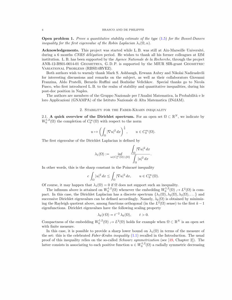
1.1. The problem. Let Ω ⊂ RN be an open set. We consider the Laplacian operator −∆ onΩ under various boundary conditions. When the relevant spectrum happens to be discrete, it isan interesting issue to provide sharp geometric estimates on associated spectral quantities like theground state energy (or first eigenvalue), the fundamental gap or more general functions of theeigenvalues. More precisely, in this manuscript we will consider the following eigenvalue problemsfor the Laplacian:
Dirichlet conditions Robin conditions−∆u = λu, in Ω,
u = 0, on ∂Ω,
−∆u = λu, in Ω,
α u+∂u
∂ν= 0, on ∂Ω,
(α > 0)
Neumann conditions Steklov conditions−∆u = µu, in Ω,
u = 0, on ∂Ω,
−∆u = 0, in Ω,∂u
∂ν= σ u, on ∂Ω.
We denote by λ1(Ω), λ1(Ω, α), µ2(Ω) and σ2(Ω) the corresponding first (or first nontrivial1) eigen-value. We refer to the next sections for the precise definitions of these eiegnvalues and theirproperties. For these spectral quantities, we have the following well-known sharp inequalities:
Dirichlet case
(1.1) |Ω|2/N λ1(Ω) ≥ |B|2/N λ1(B), (Faber-Krahn inequality)
Robin case
(1.2) |Ω|2/N λ1(Ω, α) ≥ |B|2/N λ1(B,α), (Bossel-Daners inequality)
Neumann case
(1.3) |B|2/N µ2(B) ≥ |Ω|2/N µ2(Ω), (Szego-Weinberger inequality)
Steklov case
(1.4) |B|1/N σ2(B) ≥ |Ω|1/N σ2(Ω), (Brock-Weinstock inequality)
where B denotes an N−dimensional open ball. In all the previous estimates, equality holds only ifΩ is a ball.
The fact that balls can be characterized as the only sets for which equality holds in (1.1)-(1.4)naturally leads to consider the question of the stability of these inequalities. More precisely, onewould like to improve (1.1), (1.2), (1.3) and (1.4), by adding in the right-hand sides a remainderterm measuring the deviation of a set Ω from spherical symmetry.
For example, as for inequality (1.1), a typical quantitative Faber-Krahn inequality would readas follows
(1.5) |Ω|2/N λ1(Ω)− |B|2/N λ1(B) ≥ g(d(Ω)),
where:
1Observe that in the Neumann and Steklov cases, 0 is always the first eigenvalue, associated to constant eigen-functions. Thus we use the convention that σ1(Ω) = µ1(Ω) = 0. Also observe that the Robin case can be seen as an
interpolation between Neumann (corresponding to α = 0) and Dirichlet conditions (when α = +∞).

SPECTRAL INEQUALITIES IN QUANTITATIVE FORM 3
• g : [0,+∞)→ [0,+∞) is some modulus of continuity, i. e. a positive continuous increasingfunction, vanishing at 0 only;
• Ω 7→ d(Ω) is some scaling invariant asymmetry functional, i. e. a functional defined oversets such that
d(tΩ) = d(Ω), for every t > 0 and d(Ω) = 0 if and only if Ω is a ball.
Moreover, it would desirable to have quantitative enhancements which are “the best possible”, ina sense. This means that not only we have (1.5) for every set Ω, but that it is possible to find asequence of open sets Ωnn∈N ⊂ RN such that
limn→∞
(|Ωn|2/N λ1(Ωn)− |B|2/N λ1(B)
)= 0,
and
|Ωn|2/N λ1(Ωn)− |B|2/N λ1(B) ' g(d(Ωn)), as n→∞.In this case, we would say that (1.5) is sharp. In other words, the quantitative inequality (1.5) issharp if it becomes asymptotically an equality, at least for particular shapes having small deficits.
The quest for quantitative improvements of spectral inequalities has attracted an increasinginterest in the last years. To the best of our knowledge, such a quest started with the papers [48] byHansen and Nadirashvili and [63] by Melas. Both papers concern the Faber-Krahn inequality, whichis indeed the most studied case. The reader is invited to consult Section 7 for more bibliographicalreferences and comments.
The aim of this manuscript is to give quite a complete picture on recent results about quantitativeimprovements of sharp inequalities for eigenvalues of the Laplacian. Apart from the inequalitiesfor the first eigenvalues presented above, we will also take into account some other inequalitiesinvolving the second eigenvalue in the Dirichlet case, as well as the torsional rigidity. We warn thereader from the very beginning that the presentation will be limited to the Euclidean case. For thecase of manifolds, we added some comments in Section 7.
1.2. Plan of the paper. Each section is as self-contained as possible. Where it has not beenpossible to provide all the details, we have tried to provide precise references.
In Section 2 we consider the case of the Faber-Krahn inequality (1.1), while the stability of theSzego-Weinberger and Brock-Weinstock inequalities is treated in Section 4 and 5, respectively. Foreach of these sections, we first present the relevant stability result and then discuss its sharpness.
Section 3 is a sort of divertissement, which shows some applications of the quantitative Faber-Krahn inequality to estimates for the so called harmonic radius. This part of the manuscript isessentially new and is placed there because some of the results presented will be used in Section 4.
Section 6 is devoted to present the proofs of other spectral inequalities, involving the secondDirichlet eigenvalue λ2 as well. Namely, we consider the Hong-Krahn-Szego inequality for λ2 andthe Ashbaugh-Benguria inequality for the ratio λ2/λ1.
Then in Section 7 we present some comments on further bibliographical references, applicationsand miscellaneous stability results on some particular classes of Riemannian manifolds.
The work is complemented by 4 appendices, containing technical results which are used through-out the paper.
1.3. An open issue. We conclude the Introduction by pointing out that at present no quantita-tive stability results are available for the case of the Bossel-Daners inequality. We thus start byformulating the following
4 BRASCO AND DE PHILIPPIS
Open problem 1. Prove a quantitative stability estimate of the type (1.5) for the Bossel-Danersinequality for the first eigenvalue of the Robin Laplacian λ1(Ω, α).
Acknowledgements. This project was started while L. B. was still at Aix-Marseille Universite,during a 6 months CNRS delegation period. He wishes to thank all his former colleagues at I2Minstitution. L. B. has been supported by the Agence Nationale de la Recherche, through the projectANR-12-BS01-0014-01 Geometrya, G. D. P. is supported by the MIUR SIR-grant GeometricVariational Problems (RBSI14RVEZ).
Both authors wish to warmly thank Mark S. Ashbaugh, Erwann Aubry and Nikolai Nadirashvilifor interesting discussions and remarks on the subject, as well as their collaborators GiovanniFranzina, Aldo Pratelli, Berardo Ruffini and Bozhidar Velichkov. Special thanks go to NicolaFusco, who first introduced L. B. to the realm of stability and quantitative inequalities, during hispost-doc position in Naples.
The authors are members of the Gruppo Nazionale per l’Analisi Matematica, la Probabilita e leloro Applicazioni (GNAMPA) of the Istituto Nazionale di Alta Matematica (INdAM).
2. Stability for the Faber-Krahn inequality
2.1. A quick overview of the Dirichlet spectrum. For an open set Ω ⊂ RN , we indicate byW 1,2
0 (Ω) the completion of C∞0 (Ω) with respect to the norm
u 7→(ˆ
Ω
|∇u|2 dx) 1
2
, u ∈ C∞0 (Ω).
The first eigenvalue of the Dirichlet Laplacian is defined by
λ1(Ω) := infu∈C∞0 (Ω)\0
ˆΩ
|∇u|2 dxˆ
Ω
|u|2 dx.
In other words, this is the sharp constant in the Poincare inequality
c
ˆΩ
|u|2 dx ≤ˆ
Ω
|∇u|2 dx, u ∈ C∞0 (Ω).
Of course, it may happen that λ1(Ω) = 0 if Ω does not support such an inequality.
The infimum above is attained on W 1,20 (Ω) whenever the embedding W 1,2
0 (Ω) → L2(Ω) is com-pact. In this case, the Dirichlet Laplacian has a discrete spectrum λ1(Ω), λ2(Ω), λ3(Ω), . . . andsuccessive Dirichlet eigenvalues can be defined accordingly. Namely, λk(Ω) is obtained by minimiz-ing the Rayleigh quotient above, among functions orthogonal (in the L2(Ω) sense) to the first k− 1eigenfunctions. Dirichlet eigenvalues have the following scaling property
λk(tΩ) = t−2 λk(Ω), t > 0.
Compactness of the embedding W 1,20 (Ω) → L2(Ω) holds for example when Ω ⊂ RN is an open set
with finite measure.In this case, it is possible to provide a sharp lower bound on λ1(Ω) in terms of the measure of
the set: this is the celebrated Faber-Krahn inequality (1.1) recalled in the Introduction. The usualproof of this inequality relies on the so-called Schwarz symmetrization (see [49, Chapter 2]). The
latter consists in associating to each positive function u ∈W 1,20 (Ω) a radially symmetric decreasing

SPECTRAL INEQUALITIES IN QUANTITATIVE FORM 5
function u∗ ∈ W 1,20 (Ω∗), where Ω∗ is the ball centered at the origin such that |Ω∗| = |Ω|. The
function u∗ is equimeasurable with u, that is
|x : u(x) > t| = |x : u∗(x) > t|, for every t ≥ 0,
so that in particular every Lq norm of the function u is preserved. More interestingly, one has thePolya-Szego principle (see the Subsection 2.3)
(2.1)
ˆΩ∗|∇u∗|2 dx ≤
ˆΩ
|∇u|2 dx,
from which the Faber-Krahn inequality easily follows.For a connected set Ω, the first eigenvalue λ1(Ω) is simple. In other words, there exists u1 ∈
W 1,20 (Ω) \ 0 such that every solution to
−∆u = λ1(Ω)u, in Ω, u = 0, on ∂Ω,
is proportional to u1. For a ball Br of radius r, the value λ1(Br) can be explicitely computed,together with its corresponding eigenfunction. The latter is given by the radial function (see [49])
u(x) := |x|2−N
2 JN−22
(j(N−2)/2,1
r|x|).
Here Jα is a Bessel function of the first kind, solving the ODE
g′′(t) +1
tg′(t) +
(1− α2
t2
)g(t) = 0 ,
and jα,1 denotes the first positive zero of Jα. We have
(2.2) λ1(Br) =
(j(N−2)/2,1
r
)2
.
2.2. Semilinear eigenvalues and torsional rigidity. More generally, for an open set Ω ⊂ RNwith finite measure, we will consider its first semilinear eigenvalue of the Dirichlet Laplacian
(2.3) λq1(Ω) = minu∈W 1,2
0 (Ω)\0
ˆΩ
|∇u|2 dx(ˆΩ
|u|q dx) 2q
= minu∈W 1,2
0 (Ω)
ˆΩ
|∇u|2 dx : ‖u‖Lq(Ω) = 1
,
where the exponent q satisfies
(2.4) 1 ≤ q < 2∗ :=
2N
N − 2, if N ≥ 3,
+∞, if N = 2.
For every such an exponent q the embedding W 1,20 (Ω) → Lq(Ω) is compact, thus the above mini-
mization problem is well-defined. The shape functional Ω 7→ λq1(Ω) verifies the scaling law
λq1(tΩ) = tN−2− 2q N λq1(Ω),
the exponent N − 2 − (2N)/q being negative. Still by means of Schwarz symmetrization, thefollowing general family of Faber-Krahn inequalities can be derived
(2.5) |Ω|2N + 2
q−1 λq1(Ω) ≥ |B|2N + 2
q−1 λq1(B),

6 BRASCO AND DE PHILIPPIS
where B is any N−dimensional ball. Again, equality in (2.5) is possible if and only if Ω is a ball,up to a set of zero capacity. Of course, when q = 2 we are back to λ1(Ω) defined above. We alsopoint out that the quantity
T (Ω) :=1
λ11(Ω)
= maxu∈W 1,2
0 (Ω)\0
(ˆΩ
u dx
)2
ˆΩ
|∇u|2 dx,
is usually referred to as the torsional rigidity of the set Ω. In this case, we can write (2.5) in theform
(2.6) |B|−N+2N T (B) ≥ |Ω|−
N+2N T (Ω).
This is sometimes called Saint-Venant inequality. We recall that for a ball of radius R > 0 we have
(2.7) T (BR) =1
λ11(BR)
=ωN
N (N + 2)RN+2.
Remark 2.1 (Torsion function). The torsional rigidity T (Ω) can be equivalently defined throughan unconstrained convex problems, i.e.
(2.8) − T (Ω) = minu∈W 1,2
0 (Ω)
ˆΩ
|∇u|2 dx− 2
ˆΩ
u dx
.
Indeed, it is sufficient to observe that for every u ∈ W 1,20 (Ω) and t > 0, the function t u is still
admissible and thus by Young’s inequality
minu∈W 1,2
0 (Ω)
ˆΩ
|∇u|2 dx− 2
ˆΩ
u dx
= minu∈W 1,2
0 (Ω)mint>0
t2
ˆΩ
|∇u|2 dx− 2 t
ˆΩ
u dx
= minu∈W 1,2
0 (Ω)−
(ˆΩ
u dx
)2
ˆΩ
|∇u|2 dx,
which proves (2.8). The unique solution wΩ of the problem on the right-hand side in (2.8) is calledtorsion function and it satisfies
−∆wΩ = 1, in Ω, wΩ = 0, on ∂Ω.
From (2.8) and the equation satisfied by wΩ, we thus also get
T (Ω) =
ˆΩ
wΩ dx.
2.3. Some pioneering stability results. In this part we recall the quantitative estimates for theFaber-Krahn inequality by Hansen & Nadirashvili [48] and Melas [63].
First of all, as the proof of the Faber-Krahn inequality is based on the Polya-Szego principle(2.1), it is better to recall how (2.1) can be proved. By following Talenti (see [74, Lemma 1]),the proof combines the Coarea Formula, the convexity of the function t 7→ t2 and the EuclideanIsoperimetric Inequality
(2.9) |Ω|1−NN P (Ω) ≥ |B|
1−NN P (B).
SPECTRAL INEQUALITIES IN QUANTITATIVE FORM 7
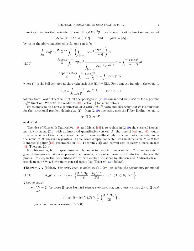
Here P ( · ) denotes the perimeter of a set. If u ∈W 1,20 (Ω) is a smooth positive function and we set
Ωt := x ∈ Ω : u(x) > t and µ(t) := |Ωt|,
by using the above mentioned tools, one can infer
ˆΩ
|∇u|2 dx Coarea=
ˆ ∞0
(ˆu=t
|∇u|2 dHN−1
|∇u|
)dt
Jensen≥
ˆ ∞0
P (Ωt)2 1ˆu=t
|∇u|−1 dHN−1dt =
ˆ ∞0
P (Ωt)2
−µ′(t)dt
Isoperimetry≥
ˆ ∞0
P (Ω∗t )2
−µ′(t)dt =
ˆΩ∗|∇u∗|2 dx,
(2.10)
where Ω∗t is the ball centered at the origin such that |Ω∗t | = |Ωt|. For a smooth function, the equality
−µ′(t) =
ˆu=t
1
|∇u|dHN−1, for a. e. t > 0,
follows from Sard’s Theorem, but all the passages in (2.10) can indeed be justified for a genuine
W 1,20 function. We refer the reader to [32, Section 2] for more details.By taking u to be a first eigenfunction of Ω with unit L2 norm and observing that u∗ is admissible
for the variational problem defining λ1(Ω∗), from (2.10) one easily gets the Faber-Krahn inequality
λ1(Ω) ≥ λ1(Ω∗),
as desired.
The idea of Hansen & Nadirashvili [48] and Melas [63] is to replace in (2.10) the classical isoperi-metric statement (2.9) with an improved quantitative version. At the time of [48] and [63], quan-titative versions of the isoperimetric inequality were availbale only for some particular sets, underthe name of Bonnesen inequalities. These cover simply connected sets in dimension N = 2 (seeBonnesen’s paper [18], generalized in [40, Theorem 2.2]) and convex sets in every dimension (see[41, Theorem 2.3]).
For this reason, both papers treat simply connected sets in dimension N = 2 or convex sets ingeneral dimensions. We now present their results, without entering at all into the details of theproofs. Rather, in the next subsection we will explain the ideas by Hansen and Nadirashvili anduse them to prove a fairly more general result (see Theorem 2.10 below).
Theorem 2.2 (Melas). For every open bounded set Ω ⊂ RN , we define the asymmetry functional
(2.11) dM(Ω) := min
max
|Ω \B1||Ω|
,|B2 \ Ω||B2|
: B1 ⊂ Ω ⊂ B2 balls
.
Then we have:
• if N = 2, for every Ω open bounded simply connected set, there exists a disc BΩ ⊂ Ω suchthat
|Ω|λ1(Ω)− |B|λ1(B) ≥ 1
C
(|Ω \BΩ||Ω|
)4
,
for some universal constant C > 0;
8 BRASCO AND DE PHILIPPIS
• if N ≥ 2 for every open bounded convex set Ω ⊂ RN we have
|Ω|2/N λ1(Ω)− |B|2/N λ1(B) ≥ 1
CdM(Ω)2N ,
for some universal constant C > 0.
Remark 2.3. In dimension N = 2 Melas’ result is indeed more general. If Ω ⊂ R2 is an openbounded set, not necessarily simply connected, then there exists an open disc BΩ such that
|Ω|λ1(Ω)− |B|λ1(B) ≥ 1
C
(|Ω∆BΩ||Ω ∪BΩ|
)4
,
for some universal constant C > 0.
For every open set Ω ⊂ RN we note
rΩ = supr > 0 : there exists x0 ∈ Ω such that Br(x0) ⊂ Ω and RΩ =
(|Ω|ωN
) 1N
.
The first quantity is usually called inradius of Ω. This is the radius of the largest ball contained inΩ.
Theorem 2.4 (Hansen-Nadirashvili). For every open set Ω ⊂ RN with finite measure, we definethe asymmetry functional
(2.12) dN (Ω) := 1− rΩ
RΩ.
Then we have:
• if N = 2 and Ω is simply connected,
|Ω|λ1(Ω)− |B|λ1(B) ≥
(π j2
0,1
250
)dN (Ω)3;
• if N ≥ 3, there exist 0 < ε < 1 and C > 0 such that for every Ω ⊂ RN open bounded convexset satisfying dN (Ω) < ε, we have
|Ω|2/N λ1(Ω)− |B|2/N λ1(B) ≥ 1
C
dN (Ω)3
| log dN (Ω)|, if N = 3,
dN (Ω)N+3
2 , if N ≥ 4.
Remark 2.5 (The role of topology). It is easy to see that the stability estimates of Theorems 2.2and 2.4 with dM and dN can not hold true without some topological assumptions on the sets. Forexample, by taking the perforated ball
Ωε = x ∈ RN : ε < |x| < 1, 0 < ε < 1,
we have
(2.13) limε0
(|Ωε|2/N λ(Ωε)− |B|2/N λ(B)
)= 0,
while
limε0
dN (Ωε) =1
2and lim
ε0dM(Ωε) ≥
1
2.
SPECTRAL INEQUALITIES IN QUANTITATIVE FORM 9
For the limit (2.13) see for example [39, Theorem 9]. These contradict Theorems 2.2 and 2.4.Observe that for N = 2 the set Ωε is not simply connected, while for N ≥ 3 it is. Thus in higherdimensions simple connectedness is still not sufficient to have stability with respect to dN or dM.
If we want to obtain a quantitative Faber-Krahn inequality for general open sets in every dimen-sion, a more flexible notion of asymmetry is the so called Fraenkel asymmetry, defined by
A(Ω) = inf
|Ω∆B||Ω|
: B ball such that |B| = |Ω|.
Observe that for every ball B such that |B| = |Ω|, we have |Ω∆B| = 2 |Ω \ B| = 2 |B \ Ω|. Thissimple facts will be used repeatedly.
It is not difficult to see that this is a weaker asymmetry functional, with respect to dN and dMabove. Indeed, we have the following.
Lemma 2.6 (Comparison between asymmetries). Let Ω ⊂ RN be an open bounded set. Then wehave
(2.14) dN (Ω) ≥ 1
2NA(Ω), dM(Ω) ≥ 1
2A(Ω) and dM(Ω) ≥ N
2NdN (Ω).
If Ω is convex, we also have
A(Ω) ≥ 1
N
(ωNN
)1/N |Ω|1/N
diam(Ω)dM(Ω)N .
Proof. By using the elementary inequality
aN − bN ≤ N aN−1 (a− b), for 0 ≤ b ≤ a,
and the definitions of rΩ, RΩ and dN (Ω), we have
(2.15) |Ω| − ωN rNΩ ≤ N |Ω|N−1N
(|Ω| 1
N − ω1N
N rΩ
)= N |Ω| dN (Ω).
We then consider a ball BrΩ(x0) ⊂ Ω and take a concentric ball B such that |B| = |Ω|. By definitionof Fraenkel asymmetry and estimate (2.15), we obtain
A(Ω) ≤ 2|Ω \ B||Ω|
≤ 2|Ω \BrΩ(x0)|
|Ω|≤ 2N dN (Ω),
and thus we get the first estimate in (2.14).
For the second one, we take a pair of balls B1 ⊂ Ω ⊂ B2 and consider the ball B1 concentric
with B1 and such that |Ω| = |B1|. Then we get
A(Ω) ≤ 2|Ω \ B1||Ω|
≤ 2|Ω \B1||Ω|
≤ 2 max
|Ω \B1||Ω|
,|B2 \ Ω||B2|
.
by taking the infimum over the admissible pairs (B1, B2) we get the second inequality in (2.14).Finally, for the third one we take again a pair of balls B1 ⊂ Ω ⊂ B2 and observe that if
rΩ ≤ RΩ/2, then we have
max
|Ω \B1||Ω|
,|B2 \ Ω||B2|
≥ |Ω \B1|
|Ω|≥ 1−
(1
2
)N≥
[1−
(1
2
)N]dN (Ω).
10 BRASCO AND DE PHILIPPIS
In the last inequality we used that dN (Ω) < 1. By taking the infimum over admissible couple ofballs, we obtain the conclusion. If on the contrary Ω is such that rΩ > RΩ/2, then by definition ofRΩ and rΩ we get
dN (Ω) =RΩ − rΩ
RΩ=|Ω|1/N − |BrΩ |1/N
|Ω|1/N≤ 1
N
|BrΩ |1/N
|Ω|1/N|Ω| − |BrΩ ||BrΩ |
≤ 1
N
|Ω| − |B1||BrΩ |
≤ 2N
N
|Ω \B1||Ω|
≤ 2N
Nmax
|Ω \B1||Ω|
,|B2 \ Ω||B2|
,
where we used that |B1| ≤ |BrΩ | ≤ |Ω|. Thus we get the conclusion in this case as well. Observethat 1− 2−N ≥ N 2−N for N ≥ 2.
Let us now assume Ω to be convex. We take a ball |B| = |Ω| such that |Ω \B|/|Ω| = A(Ω)/2. Wecan assume that A(Ω) < 1/2, otherwise the estimate is trivial by using the isodiametric inequalityand the fact that dM < 1. Then from [37, Lemma 4.2] we know that
|Ω \B| ≥ 1
2N
|Ω|diam(Ω)N
Haus(Ω, B)N .
Here Haus(E1, E2) denotes the Hausdorff distance between sets, defined by
(2.16) Haus(E1, E2) = max
supx∈E1
infy∈E2
|x− y|, supy∈E2
infx∈E1
|x− y|.
We then observe that the ball B2 := γ B contains Ω, provided
γ =RΩ + Haus(Ω, B)
RΩ.
On the other hand, by Lemma D.1 we have
rΩ ≥ RΩ −Haus(Ω, B).
Let us assume that Haus(Ω, B) < RΩ. From the definition of dM, we thus obtain
dM(Ω) ≤ max
γN − 1
γN, 1− rNΩ
RNΩ
≤ max
1− 1
γN, 1−
(1− Haus(Ω, B)
RΩ
)N
= max
1−
(1− Haus(Ω, B)
RΩ + Haus(Ω, B)
)N, 1−
(1− Haus(Ω, B)
RΩ
)N
≤ N max
Haus(Ω, B)
RΩ + Haus(Ω, B),
Haus(Ω, B)
RΩ
= N
Haus(Ω, B)
RΩ≤ N
(N
ωN
) 1N diam(Ω)
|Ω|1/NA(Ω)1/N .

SPECTRAL INEQUALITIES IN QUANTITATIVE FORM 11
This concludes the proof for Haus(Ω, B) < RΩ. If on the contrary Haus(Ω, B) ≥ RΩ, with similarcomputations we get
dM(Ω) ≤ max
γN − 1
γN, 1− rNΩ
RNΩ
≤ max
1−
(1− Haus(Ω, B)
RΩ + Haus(Ω, B)
)N, 1
≤ max
N
Haus(Ω, B)
RΩ + Haus(Ω, B), 1
≤ N
2
Haus(Ω, B)
RΩ,
and we can conclude as before.
Remark 2.7. For general open sets, the asymmetries A, dN and dM are not equivalent. We firstobserve that if Ω0 = B \ Σ, where B is a ball and Σ ⊂ B is a non-empty closed set with |Σ| = 0,then
A(Ω0) = 0 while dN (Ω0) > 0, and dM(Ω0) > 0.
Moreover, there exists a sequence of open sets Ωnn∈N ⊂ RN such that
limn→∞
dN (Ωn) = 0 and limn→∞
dM(Ωn) > 0.
Such a sequence Ωnn∈N can be constructed by attaching a long tiny tentacle to a ball, for example.
2.4. A variation on a theme by Hansen and Nadirashvili. We will now show how to adaptthe ideas by Hansen and Nadirashvili, in order to get a (non sharp) stability estimate for the generalFaber-Krahn inequality (2.5) and for general open sets with finite measure.
First of all, one needs a quantitative improvement of the isoperimetric inequality which is validfor generic sets and dimensions. Such a (sharp) quantitative isoperimetric inequality has beenproved by Fusco, Maggi and Pratelli in [43, Theorem 1.1] (see also [33, 38] for different proofs and[42] for an exhaustive review of quantitative forms of the isoperimetric inequality). This reads asfollows
(2.17) |Ω|1−NN P (Ω)− |B|
1−NN P (B) ≥ βN A(Ω)2.
An explicit value for the dimensional constant βN > 0 can be found in [38, Theorem 1.1]. Byinserting this information in the proof (2.10) of Polya-Szego inequality, one would get an estimateof the type ˆ
Ω
|∇u|2 dx−ˆ
Ω∗|∇u∗|2 dx &
ˆ ∞0
A(Ωt)2 dt.
The difficult point is to estimate the “propagation of asymmetry” from the whole domain Ω to thesuperlevel sets Ωt of the optimal function u. In other words, we would need to know that
A(Ω) ' A(Ωt), for t > 0.
Unfortunately, in general it is difficult to exclude that
A(Ωt) A(Ω), for t ' 0.
This means that the graph of u “quickly becomes round” when it detaches from the boundary ∂Ω.This may happen for example if u has a small normal derivative. For these reasons, improving thisidea is very delicate, which usually results in a (non sharp) estimate like the ones of Theorems 2.2and 2.4 and the one of Theorem 2.10 below. We refer to the discussion of Section 7.1 for otherresults of this type, previously obtained by Bhattacharya [15] and Fusco, Maggi and Pratelli [44].
The following expedient result is sometimes useful for stability issues. It states that if the measureof a subset U ⊂ Ω differs from that of Ω by an amount comparable to the asymmetry A(Ω), then

12 BRASCO AND DE PHILIPPIS
the asymmetry of U can not decrease too much. This is encoded in the following simple result,which is essentially taken from [48, Section 5].
Lemma 2.8 (Propagation of asymmetry). Let Ω ⊂ RN be an open set with finite measure. LetU ⊂ Ω be such that |U | > 0 and
(2.18)|Ω \ U ||Ω|
≤ 1
4A(Ω).
Then there holds
(2.19) A(U) ≥ 1
2A(Ω).
Proof. Let B be a ball achieving the minimum in the definition of A(U), by triangular inequalitywe get
A(U) =|U∆B||U |
≥ |Ω||U |
(|Ω∆B||Ω|
− |U∆Ω||Ω|
)≥ |Ω||U |
(|Ω∆B′||Ω|
− |B∆B′||Ω|
− |U∆Ω||Ω|
),
where B′ is a ball concentric with B and such that |B′| = |Ω|. By using that
|U∆Ω| = |Ω \ U | = |Ω| − |U | = |B′∆B|,
and the hypothesis (2.18), we get the conclusion by further noticing that |Ω| ≥ |U |.
By relying on the previous simple result, we can prove a sort of Polya-Szego inequality withremainder term. The remainder term depends on the asymmetry of Ω and on the level s of thefunction, whose corresponding superlevel set x : u(x) > s has a measure defect comparable to theasymmetry A(Ω), i.e. it satisfies (2.18).
Lemma 2.9 (Boosted Polya-Szego principle). Let Ω ⊂ RN be an open set with finite measure, such
that A(Ω) > 0. Let u ∈W 1,20 (Ω) be such that u > 0 in Ω. For every t > 0 we still denote
Ωt = x ∈ Ω : u(x) > t and µ(t) = |Ωt|.
Let s > 0 be the level defined by
(2.20) s = sup
t : µ(t) ≥ |Ω|
(1− 1
4A(Ω)
).
Then we have
(2.21)
ˆΩ
|∇u|2 dx ≥ˆ
Ω∗|∇u∗|2 dx+ cN A(Ω) |Ω|1− 2
N s2.
The dimensional constant cN > 0 is given by
cN =41/N βN N ω
1/NN
2,
and βN is the same constant appearing in (2.17).
SPECTRAL INEQUALITIES IN QUANTITATIVE FORM 13
Proof. We first observe that the level s defined by (2.20) is not 0. Indeed, the function t 7→ µ(t) isright-continuous, thus we get
limt→0+
µ(t) = µ(0) = |x ∈ Ω : u(x) > 0| = |Ω| > |Ω|(
1− 1
4A(Ω)
),
where we used the hypothesis on u and the fact that A(Ω) > 0.By using the sharp quantitative isoperimetric inequality (2.17), we have
(2.22) P (Ωt) ≥ P (Ω∗t ) + βN µ(t)N−1N A(Ωt)
2,
while by convexity of the map τ 7→ τ2 we get
P (Ωt)2 ≥ P (Ω∗t )
2 + 2P (Ω∗t )(P (Ωt)− P (Ω∗t )
)= P (Ω∗t )
2 + 2(N ω
1/NN µ(t)
N−1N
)(P (Ωt)− P (Ω∗t )
).
By collecting the previous two estimates and reproducing the proof of (2.10), we can now infer
ˆΩ
|∇u|2 dx ≥ˆ
Ω∗|∇u∗|2 dx+ c
ˆ s
0
A(Ωt)2
(µ(t)
N−1N
)2
−µ′(t)dt,(2.23)
where we set
c = 2βN N ω1/NN .
We now observe that µ is a decreasing function, thus we have
µ(t) > µ(s) ≥ |Ω|(
1− 1
4A(Ω)
), 0 < t < s.
This implies that the set Ωt verifies the hypothesis of Lemma 2.8 for 0 < t < s, since
|Ω \ Ωt||Ω|
= 1− µ(t)
|Ω|≤ 1−
(1− 1
4A(Ω)
)=
1
4A(Ω), 0 < t < s.
Thus from (2.19) we get
A(Ωt) ≥1
2A(Ω), 0 < t < s.
By inserting the previous information in (2.23) and using that
µ(t) > µ(s) ≥ |Ω|(
1− 1
4A(Ω)
)≥ |Ω|
2, 0 < t < s,
we get
ˆΩ
|∇u|2 dx ≥ˆ
Ω∗|∇u∗|2 dx+
c
4A(Ω)2
(|Ω|N−1
N
2N−1N
)2 ˆ s
0
1
−µ′(t)dt.

14 BRASCO AND DE PHILIPPIS
We then observe that by convexity of the function τ 7→ τ−1, Jensen inequality gives2
ˆ s
0
1
−µ′(t)dt ≥ s2ˆ s
0
−µ′(t) dt≥ s2
|Ω| − µ(s)≥ 4
s2
A(Ω) |Ω|,
thanks to the choice (2.20) of s. This concludes the proof.
We can now prove the following quantitative version of the general Faber-Krahn inequality (2.5).The standard case of the first eigenvalue of the Dirichlet Laplacian corresponds to taking q = 2.Though the exponent on the Fraenkel asymmetry is not sharp, the interest of the result lies in thecomputable constant. Moreover, the proof is quite simple and it is based on the ideas by Hansen& Nadirashvili. We also use Kohler-Jobin inequality (see Appendix A) to reduce to the case ofthe torsional rigidity. This reduction trick has been first introduced by Brasco, De Philippis andVelichkov in [21].
Theorem 2.10. Let 1 ≤ q < 2∗, there exists an explicit constant τN,q > 0 such that for every openset Ω ⊂ RN with finite measure, we have
(2.24) |Ω|2N + 2
q−1 λq1(Ω)− |B|2N + 2
q−1 λq1(B) ≥ τN,q A(Ω)3.
Proof. Since inequality (2.24) is scaling invariant, we can suppose that |Ω| = 1. By PropositionA.1 with
g(t) = t3 and d(Ω) = A(Ω),
it is sufficient to prove (2.24) for the torsional rigidity. In other words, we just need to prove thefollowing quantitative Saint-Venant inequality
(2.25) T (Ω∗)− T (Ω) ≥ τ A(Ω)3,
where as always Ω∗ is the ball centered at the origin such that |Ω∗| = |Ω| = 1. Of course, we cansuppose that A(Ω) > 0, otherwise there is nothing to prove. Without loss of generality, we can alsosuppose that
(2.26) T (Ω) ≥ T (Ω∗)
2.
Indeed, if the latter is not satisfied, then (2.25) trivially holds with constant τ = T (Ω∗)/16, thanksto the fact that A(Ω) < 2.
Let wΩ ∈W 1,20 (Ω) be the torsion function of Ω (recall Remark 2.1), then we know
T (Ω) =
ˆΩ
wΩ dx =
ˆΩ
|∇wΩ|2 dx.
Moreover, by standard elliptic regularity we know that wΩ ∈ C∞(Ω) ∩ L∞(Ω). By recalling that|Ω| = 1 and (2.26), we get
T (Ω∗)
2≤ T (Ω) =
ˆΩ
wΩ dx ≤ ‖wΩ‖L∞(Ω).
2In the second inequality, we used that for a monotone non-decreasing function fˆ b
af ′(t) dt ≤ f(b)− f(a), for a < b.

SPECTRAL INEQUALITIES IN QUANTITATIVE FORM 15
We now take s as in (2.20), from (2.21) and the definition of torsional rigidity we get
T (Ω) ≤
(ˆΩ∗w∗Ω dx
)2
ˆΩ∗|∇w∗Ω|2 dx+ cN A(Ω) s2
≤ T (Ω∗)
1 +cN A(Ω) s2ˆΩ∗|∇w∗Ω|2 dx
−1
,
that isT (Ω∗)
T (Ω)− 1 ≥ cN A(Ω) s2ˆ
Ω∗|∇w∗Ω|2 dx
.
With simple manipulations, by using´
Ω∗|∇w∗Ω|2 ≤
´Ω|∇wΩ|2 = T (Ω), we get
(2.27) T (Ω∗)− T (Ω) ≥ cN A(Ω) s2.
We then set
(2.28) s0 =T (Ω∗)
16
N + 2
3N + 2A(Ω),
and observe that s0 < T (Ω∗)/4. We have to distinguish two cases.
First case: s ≥ s0. This is the easy case, as from (2.27) we directly get (2.25), with constant
τ =cN256
T (Ω∗)2
(N + 2
3N + 2
)2
,
and we recall that cN is as in Lemma 2.9.
Second case: s < s0. In this case, by definition (2.20) of s we get
(2.29) µ(s0) <
(1− 1
4A(Ω)
).
We also observe that µ(s0) > 0, since s0 < T (Ω∗)/4 ≤ 1/2 ‖wΩ‖L∞ by the discussion above. Wenow want to work with this level s0. We haveˆ
Ωs0
(wΩ − s0)+ dx =
ˆΩ
(wΩ − s0)+ dx ≥ˆ
Ω
wΩ dx− s0 = T (Ω)− s0.(2.30)
Observe that the right-hand side is strictly positive, since s0 < T (Ω) thanks to (2.28) and (2.26). We
have (wΩ− s0)+ ∈W 1,20 (Ωs0), thus from the variational characterization of T (Ω), the Saint-Venant
inequality and (2.30)
T (Ω) =
(ˆΩ
wΩ dx
)2
ˆΩ
|∇wΩ|2 dx≤
(ˆΩ
wΩ dx
)2
ˆΩ
|∇(wΩ − s0)+|2 dx≤ T (Ωs0)
ˆ
Ω
wΩ dxˆΩ
(w − s0)+ dx
2
≤ T (Ω∗)µ(s0)N+2N
(1− s0
T (Ω)
)−2
.
Since s0 satisfies (2.29), from the previous estimate and again (2.26) we can infer
(2.31)
(1− 1
4A(Ω)
)−N+2N(
1− s0
T (Ω∗)
)2
− 1 ≤ T (Ω∗)
T (Ω)− 1 ≤ 2
T (Ω∗)
(T (Ω∗)− T (Ω)
).
16 BRASCO AND DE PHILIPPIS
We then observe that(1− 1
4A(Ω)
)−N+2N
≥ 1 +N + 2
4NA(Ω) and
(1− s0
T (Ω∗)
)2
≥ 1− 2 s0
T (Ω∗).
Thus from (2.31) we get
T (Ω∗)− T (Ω) ≥ T (Ω∗)
2
[(1 +
N + 2
4NA(Ω)
) (1− 2 s0
T (Ω∗)
)− 1
].(2.32)
We now recall the definition (2.28) of s0 and finally estimate(1 +
N + 2
4NA(Ω)
)(1− 2 s0
T (Ω∗)
)− 1 ≥ N + 2
8NA(Ω).
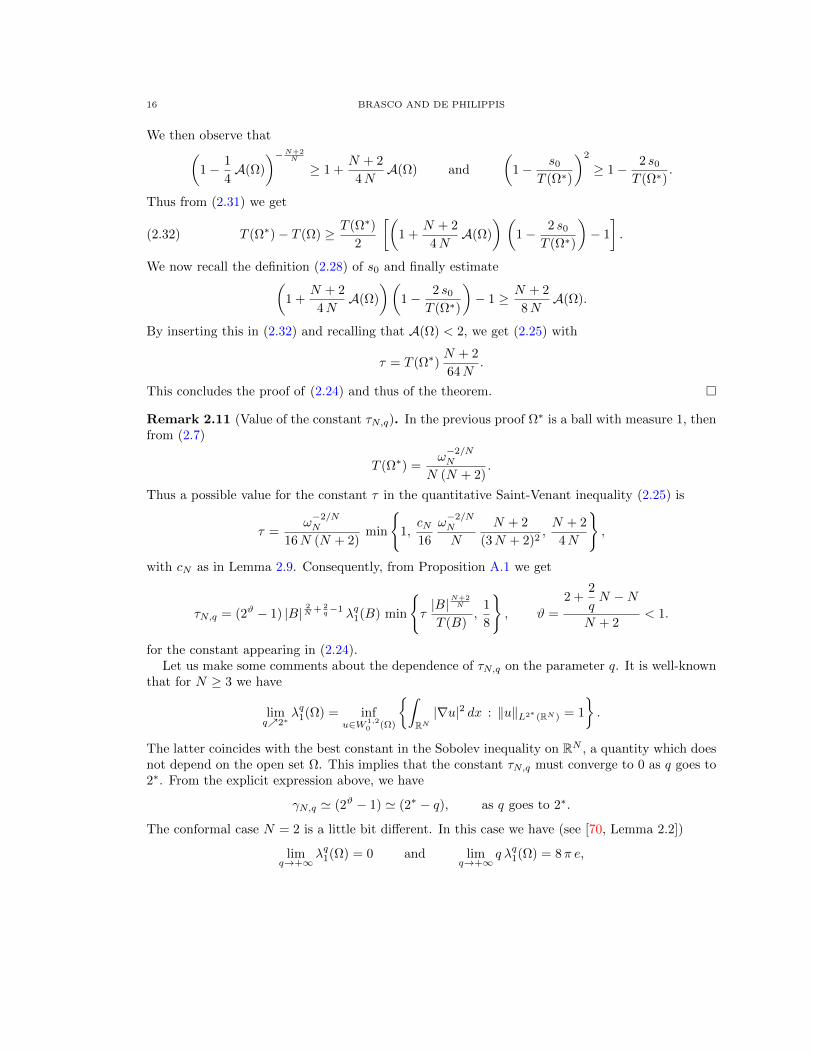
By inserting this in (2.32) and recalling that A(Ω) < 2, we get (2.25) with
τ = T (Ω∗)N + 2
64N.
This concludes the proof of (2.24) and thus of the theorem.
Remark 2.11 (Value of the constant τN,q). In the previous proof Ω∗ is a ball with measure 1, thenfrom (2.7)
T (Ω∗) =ω−2/NN
N (N + 2).
Thus a possible value for the constant τ in the quantitative Saint-Venant inequality (2.25) is
τ =ω−2/NN
16N (N + 2)min
1,cN16
ω−2/NN
N
N + 2
(3N + 2)2,N + 2
4N
,
with cN as in Lemma 2.9. Consequently, from Proposition A.1 we get
τN,q = (2ϑ − 1) |B|2N + 2
q−1 λq1(B) min
τ|B|N+2
N
T (B),
1
8
, ϑ =
2 +2
qN −N
N + 2< 1.
for the constant appearing in (2.24).Let us make some comments about the dependence of τN,q on the parameter q. It is well-known
that for N ≥ 3 we have
limq2∗
λq1(Ω) = infu∈W 1,2
0 (Ω)
ˆRN|∇u|2 dx : ‖u‖L2∗ (RN ) = 1
.
The latter coincides with the best constant in the Sobolev inequality on RN , a quantity which doesnot depend on the open set Ω. This implies that the constant τN,q must converge to 0 as q goes to2∗. From the explicit expression above, we have
γN,q ' (2ϑ − 1) ' (2∗ − q), as q goes to 2∗.
The conformal case N = 2 is a little bit different. In this case we have (see [70, Lemma 2.2])
limq→+∞
λq1(Ω) = 0 and limq→+∞
q λq1(Ω) = 8π e,

SPECTRAL INEQUALITIES IN QUANTITATIVE FORM 17
for every open bounded set Ω. By observing that for N = 2 we have ϑ = 1/q, the asymptoticbehaviour of the constant γ2,q is then given by
γ2,q '(
21q − 1
)λq1(B) ' 1
q2, as q goes to +∞.
2.5. The Faber-Krahn inequality in sharp quantitative form. As simple and general as itis, the previous result is however not sharp. Indeed, Bhattacharya and Weitsman [16, Section 8]and Nadirashvili [65, page 200] indipendently conjectured the following.
BWN Conjecture. There exists a dimensional constant C > 0 such that
|Ω|2/N λ(Ω)− |B|2/N λ(B) ≥ 1
CA(Ω)2.
After some attempts and intermediate results, this has been proved by Brasco, De Philippis andVelichkov in [21]. This follows by choosing q = 2 in the statement below, which is again valid inthe more general case of the first semilinear eigenvalues. We remark that this time the constantappearing in the estimate is not explicit. However, we can trace its dependence on q, which is thesame as that of γN,q in Remark 2.11.
Theorem 2.12. Let 1 ≤ q < 2∗. There exists a constant γN,q, depending only on the dimensionN and q, such that for every open set Ω ⊂ RN with finite measure we have
(2.33) |Ω|2N + 2
q−1 λq1(Ω)− |B|2N + 2
q−1 λq1(B) ≥ γN,q A(Ω)2.
The proof of this result is quite long and technical. We will briefly describe the main ideas andsteps of the proof, referring the reader to the original paper [21] for all the details.
Let us stress that differently from the previous results, the proof of Theorem 2.12 does not rely onquantitative versions of the Polya-Szego principle, since this technique seems very hard to implementin sharp form (as explained at the beginning of Subsection 2.4). On the contrary, the main core isbased on the selection principle introduced by Cicalese and Leonardi in [33] to give a new proof ofthe aforementioned quantitative isoperimetric inequality (2.22).
The selection principle turns out to be a very flexible technique and after the paper [33] it hasbeen applied to a wide variety of geometric problems, see for instance [1, 17] and [36].
Let us now explain the main steps of the proof of Theorem 2.12.
Step 1: reduction to the torsional rigidity
We start by observing that by Proposition A.1 it is sufficient to prove the result for the torsionalrigidity. In other words, it is sufficient to prove
(2.34) T (B1)− T (Ω) ≥ 1
CA(Ω)2, for Ω ⊂ RN such that |Ω| = |B1|,
where C is a dimensional constant and B1 is the ball of radius 1 centered at the origin.
Step 2: sharp stability for nearly spherical sets
One then observes that if Ω is a sufficiently smooth perturbation of B1, then (2.34) can be proved bymeans of a second order expansion argument. More precisely, in this step we consider the followingclass of sets.

18 BRASCO AND DE PHILIPPIS
Definition 2.13. An open bounded set Ω ⊂ RN is said nearly spherical of class C2,γ parametrizedby ϕ, if there exists ϕ ∈ C2,γ(∂B1) with ‖ϕ‖L∞ ≤ 1/2 and such that ∂Ω is represented by
∂Ω =x ∈ RN : x = (1 + ϕ(y)) y, for y ∈ ∂B1
.
For nearly spherical sets, we then have the following quantitative estimate. The proof relies ona second order Taylor expansion for the torsional rigidity, see [34] and [21, Appendix A].
Proposition 2.14. Let 0 < γ ≤ 1. Then there exists δ1 = δ1(N, γ) > 0 such that if Ω is a nearlyspherical set of class C2,γ parametrized by ϕ with
‖ϕ‖C2,γ(∂B1) ≤ δ1, |Ω| = |B1| and xΩ :=
Ω
x dx = 0,
then
(2.35) T (B1)− T (Ω) ≥ 1
32N2‖ϕ‖2L2(∂B1) .
Remark 2.15. It is not difficult to see that (2.35) implies (2.34) for the class of sets under con-sideration. Indeed, we have
‖ϕ‖2L2(∂B1) ≥1
N ωN
(ˆ∂B1
|ϕ| dHN−1
)2
,
and
A(Ω) ≤ |Ω∆B1||Ω|
=1
N ωN
ˆ∂B1
|1− (1 + ϕ)N | dHN−1 ' 1
ωN
ˆ∂B1
|ϕ| dHN−1.
Let us record that actually inequality (2.35) holds true in a stronger form, where the L2 norm of ϕis replaced by its W 1/2,2(∂Ω) norm, see [21, Theorem 3.3].
Step 3: reduction to the small asymmetry regime
This simple step permits to reduce the task to proving (2.34) for sets having suitably small Fraenkelasymmetry. Namely, we have the following result.
Proposition 2.16. Let us suppose that there exist ε > 0 and c > 0 such that
T (B1)− T (Ω) ≥ cA(Ω)2, for Ω such that |Ω| = |B1| and A(Ω) < ε.
Then (2.34) holds true with1
C= minc, ε τ
where τ > 0 is the dimensional constant appearing in (2.25).
Proof. Once we have Theorem 2.10 at our disposal, the proof is straightforward. Indeed, if A(Ω) ≥ε, then by (2.25) we get
T (B1)− T (Ω) ≥ τ A(Ω)3 ≥ ε τ A(Ω)2,
as desired. However, let us point out that for the proof of this result it is not really needed the powerlaw relation given by (2.25), it would be sufficient to know that A(Ω)→ 0 as T (B1)−T (Ω)→ 0.
Step 4: reduction to bounded sets
We can still make a further reduction, namely we can restrict ourselves to prove (2.34) for sets withuniformly bounded diameter. This is a consequence of the following expedient result.
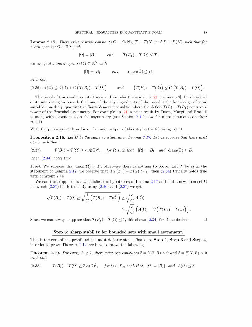
SPECTRAL INEQUALITIES IN QUANTITATIVE FORM 19
Lemma 2.17. There exist positive constants C = C(N), T = T (N) and D = D(N) such that forevery open set Ω ⊂ RN with
|Ω| = |B1| and T (B1)− T (Ω) ≤ T ,
we can find another open set Ω ⊂ RN with
|Ω| = |B1| and diam(Ω) ≤ D,
such that
(2.36) A(Ω) ≤ A(Ω) + C(T (B1)− T (Ω)
)and
(T (B1)− T (Ω)
)≤ C
(T (B1)− T (Ω)
).
The proof of this result is quite tricky and we refer the reader to [21, Lemma 5.3]. It is howeverquite interesting to remark that one of the key ingredients of the proof is the knowledge of somesuitable non-sharp quantitative Saint-Venant inequality, where the deficit T (Ω)− T (B1) controls apower of the Fraenkel asymmetry. For example, in [21] a prior result by Fusco, Maggi and Pratelliis used, with exponent 4 on the asymmetry (see Section 7.1 below for more comments on theirresult).
With the previous result in force, the main output of this step is the following result.
Proposition 2.18. Let D be the same constant as in Lemma 2.17. Let us suppose that there existc > 0 such that
(2.37) T (B1)− T (Ω) ≥ cA(Ω)2, for Ω such that |Ω| = |B1| and diam(Ω) ≤ D.
Then (2.34) holds true.
Proof. We suppose that diam(Ω) > D, otherwise there is nothing to prove. Let T be as in thestatement of Lemma 2.17, we observe that if T (B1) − T (Ω) > T , then (2.34) trivially holds truewith constant T /4.
We can thus suppose that Ω satisfies the hypotheses of Lemma 2.17 and find a new open set Ωfor which (2.37) holds true. By using (2.36) and (2.37) we get√
T (B1)− T (Ω) ≥√
1
C
(T (B1)− T (Ω)
)≥√c
CA(Ω)
≥√c
C
(A(Ω)− C
(T (B1)− T (Ω)
)).
Since we can always suppose that T (B1)− T (Ω) ≤ 1, this shows (2.34) for Ω, as desired.
Step 5: sharp stability for bounded sets with small asymmetry
This is the core of the proof and the most delicate step. Thanks to Step 1, Step 3 and Step 4,in order to prove Theorem 2.12, we have to prove the following.
Theorem 2.19. For every R ≥ 2, there exist two constants c = c(N,R) > 0 and ε = ε(N,R) > 0such that
(2.38) T (B1)− T (Ω) ≥ cA(Ω)2, for Ω ⊂ BR such that |Ω| = |B1| and A(Ω) ≤ ε.

20 BRASCO AND DE PHILIPPIS
The idea of the proof is to proceed by contradiction. Indeed, let us suppose that (2.38) is false.Thus we may find a sequence of open sets Ωjj∈N ⊂ BR(0) such that
(2.39) |Ωj | = |B1|, εj := A(Ωj)→ 0 and T (B1)− T (Ωj) ≤ cA(Ωj)2,
with c > 0 as small as we wish. The idea is to use a variational procedure to replace the sequenceΩjj∈N with an “improved” one Ujj∈N which still contradicts (2.38) and enjoys some additionalsmoothness properties.
In the spirit of the celebrated Ekeland’s variational principle, the idea is to select such a sequencethrough some penalized minimization problem. Roughly speaking we look for sets Uj which solvethe following
(2.40) minT (B1)− T (Ω) +
√ε2j + η (A(Ω)− εj)2 : Ω ⊂ BR, |Ω| = |B1(0)|
,
where η > 0 is a suitably small parameter, which will allow to get the final contradiction.One can easily show that the sequence Uj still contradicts (2.38) and that A(Uj) → 0. Relying
on the minimality of Uj , one then would like to show that the L1 convergence to B1 can be improvedto a C2,γ convergence. If this is the case, then the stability result for smooth nearly spherical setsProposition 2.14 applies and shows that (2.39) cannot hold true if c in (2.39) is sufficiently small.
The key point is thus to prove (uniform) regularity estimates for sets solving (2.40). For this, firstone would like to get rid of volume constraints applying some sort of Lagrange multiplier principleto show that Uj solves
(2.41) minT (B1)− T (Ω) +
√ε2j + η (A(Ω)− εj)2 + Λ |Ω| : Ω ⊂ BR
.
Then, recalling the formulation (2.8) for −T (Ω), we can take advantage of the fact that we areconsidering a “min–min” problem. Thus the previous problem is equivalent to require that thetorsion function wj := wUj of Uj minimizesˆ
RN|∇v|2 dx− 2
ˆRN
v dx+ Λ∣∣v > 0
∣∣+√ε2j + η (A(v > 0)− εj)2,(2.42)
among all functions with compact support in BR. Since we are now facing a perturbed free boundarytype problem, we aim to apply the techniques of Alt and Caffarelli [4] (see also [28, 29]) to showthe regularity of ∂Uj = ∂uj > 0 and to obtain the smooth convergence of Uj to B1.
This is the general strategy, but several non-trivial modifications have to be done to the abovesketched proof. A first technical difficulty is that no global Lagrange multiplier principle is available.Indeed, since by scaling
−T (tΩ)− = −tN+2 T (Ω) and |tΩ| = tN |Ω|, t > 0,
by a simple scaling argument one sees that the infimum of the energy in (2.41) would be identically−∞ in the uncostrained case. This can be fixed by following [2] and replacing the term Λ |Ω| witha term of the form f(|Ω| − |B1|), for a suitable strictly increasing function f vanishing at 0 only.
A more serious obstruction is due to the lack of regularity of the Fraenkel asymmetry. Althoughsolutions to (2.42) enjoy some mild regularity properties, we cannot expect ∂uj > 0 to be smooth.Indeed, by formally computing the optimality condition3 of (2.42) and assuming that B1 is the
3That is differentiating the functional along perturbation of the form vt = uj (Id + tV ) where V is a smooth
vector field.

SPECTRAL INEQUALITIES IN QUANTITATIVE FORM 21
unique optimal ball for the Fraenkel asymmetry of wj > 0, one gets that wj should satisfy∣∣∣∣∂wj∂ν
∣∣∣∣2 = Λ +η (A(wj > 0)− εj)√
ε2j + η (A(wj > 0)− εj)2
(1RN\B1
− 1B1
)on ∂wj > 0,
where 1A denotes the characteristic function of a set A and ν is the outer normal versor. Thismeans that the normal derivative of wj is discontinuous at points where Uj = wj > 0 crosses
∂B1. Since classical elliptic regularity implies that if ∂Uj is C1,γ then uj ∈ C1,γ(Uj), it is clearthat the sets Uj can not enjoy too much smoothness properties. In particular, it seems difficult toobtain the regularity C2,γ needed to apply Proposition 2.14.
To overcome this difficulty, we replace the Fraenkel asymmetry with a new asymmetry functional,which behaves like a squared L2 distance between the boundaries and whose definition is inspiredby [3]. For a bounded set Ω ⊂ RN , this is defined by
α(Ω) =
ˆΩ∆B1(xΩ)
∣∣1− |x− xΩ|∣∣ dx,
where xΩ is the barycenter of Ω. Notice that α(Ω) = 0 if and only if Ω is a ball of radius 1.This asymmetry is differentiable with respect to the variations needed to compute the optimal-ity conditions (differently from the Fraenkel asymmetry), moreover it enjoys the following crucialproperties:
(i) there exists a constant C1 = C1(N) > 0 such that for every Ω
(2.43) C1 α(Ω) ≥ |Ω∆B1(xΩ)|2;
(ii) there exists two constants δ2 = δ2(N) > 0 and C2 = C2(N) > 0 such that for every nearlyspherical set Ω parametrized by ϕ with ‖ϕ‖L∞ ≤ δ2, we have
(2.44) α(Ω) ≤ C2 ‖ϕ‖2L2(∂B1).
By using the strategy described above and replacing A(Ω) with α(Ω), one can obtain the following.
Proposition 2.20 (Selection Principle). Let R ≥ 2 then there exists η = η(N,R) > 0 such that if0 < η ≤ η(N,R) and Ωjj∈N ⊂ RN verify
|Ωj | = |B1| and εj := α(Ωj)→ 0, while T (B1)− T (Ωj) ≤ η4 εj ,
then we can find a sequence of smooth open sets Ujj∈N ⊂ BR satisfying:
(i) |Uj | = |B1|;(ii) xUj = 0;
(iii) ∂Uj are converging to ∂B1 in Ck for every k;(iv) there holds
lim supj→∞
T (B1)− T (Uj)
α(Uj)≤ C3 η,
for some constant C3 = C3(N,R) > 0.
In turn, this permits to prove the following alternative version of Theorem 2.19, by following thecontradiction scheme sketched above. Indeed, we can apply Proposition 2.14 to the sets Uj and(2.44) in order to get
1
32N2≤ lim sup
j→∞
T (B1)− T (Uj)
‖ϕj‖L2(∂B)≤ C2 lim sup
j→∞
T (B1)− T (Uj)
α(Uj)≤ C2 C3 η,
22 BRASCO AND DE PHILIPPIS
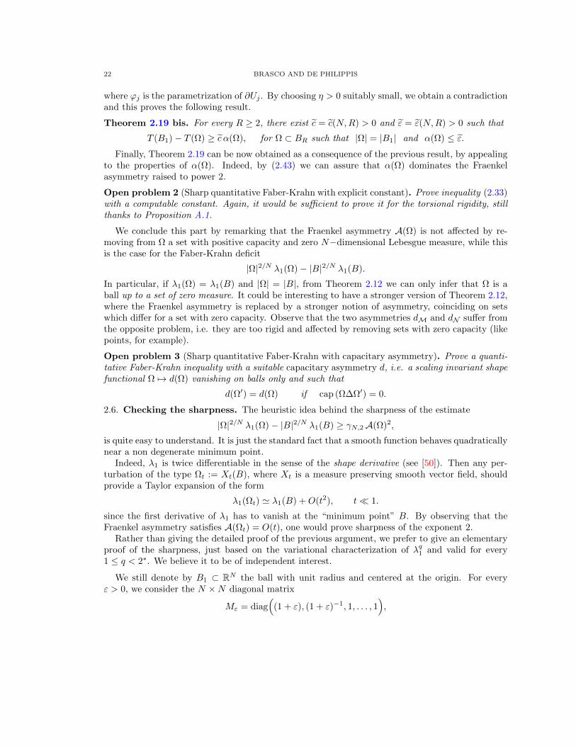
where ϕj is the parametrization of ∂Uj . By choosing η > 0 suitably small, we obtain a contradictionand this proves the following result.
Theorem 2.19 bis. For every R ≥ 2, there exist c = c(N,R) > 0 and ε = ε(N,R) > 0 such that
T (B1)− T (Ω) ≥ c α(Ω), for Ω ⊂ BR such that |Ω| = |B1| and α(Ω) ≤ ε.Finally, Theorem 2.19 can be now obtained as a consequence of the previous result, by appealing
to the properties of α(Ω). Indeed, by (2.43) we can assure that α(Ω) dominates the Fraenkelasymmetry raised to power 2.
Open problem 2 (Sharp quantitative Faber-Krahn with explicit constant). Prove inequality (2.33)with a computable constant. Again, it would be sufficient to prove it for the torsional rigidity, stillthanks to Proposition A.1.
We conclude this part by remarking that the Fraenkel asymmetry A(Ω) is not affected by re-moving from Ω a set with positive capacity and zero N−dimensional Lebesgue measure, while thisis the case for the Faber-Krahn deficit
|Ω|2/N λ1(Ω)− |B|2/N λ1(B).
In particular, if λ1(Ω) = λ1(B) and |Ω| = |B|, from Theorem 2.12 we can only infer that Ω is aball up to a set of zero measure. It could be interesting to have a stronger version of Theorem 2.12,where the Fraenkel asymmetry is replaced by a stronger notion of asymmetry, coinciding on setswhich differ for a set with zero capacity. Observe that the two asymmetries dM and dN suffer fromthe opposite problem, i.e. they are too rigid and affected by removing sets with zero capacity (likepoints, for example).
Open problem 3 (Sharp quantitative Faber-Krahn with capacitary asymmetry). Prove a quanti-tative Faber-Krahn inequality with a suitable capacitary asymmetry d, i.e. a scaling invariant shapefunctional Ω 7→ d(Ω) vanishing on balls only and such that
d(Ω′) = d(Ω) if cap (Ω∆Ω′) = 0.
2.6. Checking the sharpness. The heuristic idea behind the sharpness of the estimate
|Ω|2/N λ1(Ω)− |B|2/N λ1(B) ≥ γN,2A(Ω)2,
is quite easy to understand. It is just the standard fact that a smooth function behaves quadraticallynear a non degenerate minimum point.
Indeed, λ1 is twice differentiable in the sense of the shape derivative (see [50]). Then any per-turbation of the type Ωt := Xt(B), where Xt is a measure preserving smooth vector field, shouldprovide a Taylor expansion of the form
λ1(Ωt) ' λ1(B) +O(t2), t 1.
since the first derivative of λ1 has to vanish at the “minimum point” B. By observing that theFraenkel asymmetry satisfies A(Ωt) = O(t), one would prove sharpness of the exponent 2.
Rather than giving the detailed proof of the previous argument, we prefer to give an elementaryproof of the sharpness, just based on the variational characterization of λq1 and valid for every1 ≤ q < 2∗. We believe it to be of independent interest.
We still denote by B1 ⊂ RN the ball with unit radius and centered at the origin. For everyε > 0, we consider the N ×N diagonal matrix
Mε = diag(
(1 + ε), (1 + ε)−1, 1, . . . , 1),
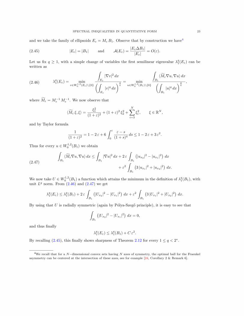
SPECTRAL INEQUALITIES IN QUANTITATIVE FORM 23
and we take the family of ellipsoids Eε = MεB1. Observe that by construction we have4
(2.45) |Eε| = |B1| and A(Eε) =|Eε∆B1||Eε|
= O(ε).
Let us fix q ≥ 1, with a simple change of variables the first semilinear eigenvalue λq1(Eε) can bewritten as
λq1(Eε) = minv∈W 1,2
0 (Eε)\0
ˆEε
|∇v|2 dx(ˆEε
|v|q dx) 2q
= minu∈W 1,2
0 (B1)\0
ˆB1
〈Mε∇u,∇u〉 dx(ˆB1
|u|q dx) 2q
,(2.46)
where Mε = M−1ε M−1
ε . We now observe that
〈Mε ξ, ξ〉 =ξ21
(1 + ε)2+ (1 + ε)2 ξ2
2 +N∑i=3
ξ2i , ξ ∈ RN ,
and by Taylor formula
1
(1 + ε)2= 1− 2 ε+ 6
ˆ ε
0
ε− s(1 + s)4
ds ≤ 1− 2 ε+ 3 ε2.
Thus for every u ∈W 1,20 (B1) we obtain
ˆB1
〈Mε∇u,∇u〉 dx ≤ˆB1
|∇u|2 dx+ 2 ε
ˆB1
(|ux2 |2 − |ux1 |2
)dx
+ ε2
ˆB1
(3 |ux1 |2 + |ux2 |2
)dx.
(2.47)
We now take U ∈W 1,20 (B1) a function which attains the minimum in the definition of λq1(B1), with
unit Lq norm. From (2.46) and (2.47) we get
λq1(Eε) ≤ λq1(B1) + 2 ε
ˆB1
(|Ux2 |2 − |Ux1 |2
)dx+ ε2
ˆB1
(3 |Ux1 |2 + |Ux2 |2
)dx.
By using that U is radially symmetric (again by Polya-Szego principle), it is easy to see thatˆB1
(|Ux2 |2 − |Ux1 |2
)dx = 0,
and thus finally
λq1(Eε) ≤ λq1(B1) + C ε2.
By recalling (2.45), this finally shows sharpness of Theorem 2.12 for every 1 ≤ q < 2∗.
4We recall that for a N−dimensional convex sets having N axes of symmetry, the optimal ball for the Fraenkelasymmetry can be centered at the intersection of these axes, see for example [24, Corollary 2 & Remark 6].

24 BRASCO AND DE PHILIPPIS
3. Intermezzo: quantitative estimates for the harmonic radius
In this section we present an application of the quantitative Faber-Krahn inequality to estimatesfor the so-called harmonic radius. Apart from being interesting in themselves, some of these resultswill be useful in the next section.
Definition 3.1 (Harmonic radius). We denote by GΩx the Green function of Ω with singularity at
x ∈ Ω, i.e.
−∆GΩx = δx in Ω, GΩ
x = 0 on ∂Ω,
where δx is the Dirac Delta centered at x. We recall that
GΩx (y) = ςN
(ΓN (|x− y|)−HΩ
x (y)),
where:
• ςN is the following dimensional constant
ς2 =1
2π, ςN =
1
(N − 2)N ωN, for N ≥ 3;
• ΓN is the function defined on (0,+∞)
Γ2(t) = − log t, ΓN (t) = t2−N , for N ≥ 3;
• HΩx is the regular part, which solves
∆HΩx = 0 in Ω, HΩ
x = ΓN (|x− ·|) on ∂Ω.
With the notation above, the harmonic radius of Ω is defined by
(3.1) IΩ := supx∈Ω
Γ−1N (HΩ
x (x)).
We refer the reader to the survey paper [11] for a comprehensive study of the harmonic radius.
Remark 3.2 (Scaling properties). It is not difficult to see that IΩ scales like a length. This followsfrom the fact that for every t > 0
(3.2) GtΩx (y) = t2−N GΩ
x/t
(yt
), y 6= x ∈ tΩ.
Then in dimension N ≥ 3 we get
HtΩx (y) = t2−N HΩ
x/t
(yt
)and thus ItΩ := sup
x∈tΩ
(t2−N HΩ
x/t
(xt
)) 12−N
= t IΩ.
In dimension 2 we proceed similarly, by observing that from (3.2)
HtΩx (y) = − log t+HΩ
x/t
(xt
).
For our purposes, it is useful to recall the following spectral inequality.
Theorem 3.3 (Hersch-Polya-Szego inequality). Let Ω ⊂ RN be an open bounded set. Then wehave the scaling invariant estimate
(3.3) λ1(Ω) ≤ λ1(B1)
I2Ω
.
Equality in (3.3) is attained for balls only.
SPECTRAL INEQUALITIES IN QUANTITATIVE FORM 25
Proof. Under these general assumptions, the result is due to Hersch and is proved by using harmonictransplation, a technique introduced in [51]. The original result by Polya and Szego is for N = 2and Ω simply connected, by means of conformal transplantation. We present their proof below, byreferring to [11, Section 6] for the general case.
Thus, let us take N = 2 and Ω simply connected. Without loss of generality, we can assume|Ω| = π. For every x0 ∈ Ω, we consider the holomorphic isomorphism given by the RiemannMapping Theorem
fx0: Ω→ B1,
such that5 fx0(x0) = 0. Then we have the following equivalent characterization for the harmonic
radius
(3.4) IΩ = supx0∈Ω
∣∣(f−1x0
)′(0)∣∣ = sup
x0∈Ω
1
|f ′x0(x0)|
.
Here f ′ denotes the complex derivative. Indeed, with the notation above the Green function of Ωwith singularity at x0 is given by
GΩx0
(y) = − 1
2πlog |fx0
(y)|, y ∈ Ω \ x0.
We can rewrite it as
GΩx0
(y) = − 1
2πlog |fx0
(y)− fx0(x0)| = − 1
2πlog |y − x0| −
1
2πlog|fx0
(y)− fx0(x0)|
|y − x0|.
By recalling the definition (3.1) of harmonic radius, we get
IΩ = supx0∈Ω
limy→x0
exp
(− log
|fx0(y)− fx0(x0)||y − x0|
)= supx0∈Ω
1
|f ′x0(x0)|
,
which proves (3.4).
We now prove (3.3). Let u ∈ W 1,20 (B1) be the first positive Dirichlet eigenfunction of B1, with
unit L2 norm. For x0 ∈ Ω, we consider fx0: Ω→ B1 as above, then we set
v = u f.
By conformality we preserve the Dirichlet integral, i.e.ˆΩ
|∇v|2 dx =
ˆB1
|∇u|2 dx = λ1(B1).
On the other hand, by the change of variable formula we haveˆΩ
|v|2 dx =
ˆB1
|u|2 |(f−1x0
)′|2 dx.
We now observe that |(f−1x0
)′|2 is sub-harmonic, thus the function
(3.5) Φ(%) =1
2π %
ˆ|x|=%
|(f−1x0
)′|2 dH1,
is non-decreasing. In particular, we have
Φ(%) ≥ Φ(0) = |(f−1x0
)′(0)|2.
5We recall that this is uniquely defined, up to a rotation.
26 BRASCO AND DE PHILIPPIS
Thus we obtain ˆΩ
|v|2 dx =
ˆΩ
|u|2 |(f−1x0
)′|2 dx = 2π
ˆ 1
0
u2 %Φ(%) d%
≥(
2π
ˆ 1
0
u2 % d%
)|(f−1
x0)′(0)|2 = |(f−1
x0)′(0)|2,
since u has unitary L2 norm. By using the variational characterization of λ1(Ω), this finally shows
|(f−1x0
)′(0)|2 λ1(Ω) ≤ λ1(B1).
By taking the supremum over Ω and using (3.4), we get the conclusion.
Remark 3.4 (Conformal radius). Historically, the quantity
maxx0∈Ω
∣∣(f−1x0
)′(0)∣∣ = max
x0∈Ω
1
|f ′x0(x0)|
,
has been first introduced under the name conformal radius of Ω. The definition of harmonic radiusis due to Hersch [51], as we have seen this gives a genuine extension to general sets of the conformalradius.
Among open sets with given measure, the harmonic radius is maximal on balls. By recallingthat for a ball the harmonic radius coincides with the radius tout court, we thus have the scalinginvariant estimate
(3.6)|Ω|2/N
I2Ω
≥ ω2/NN .
This can be deduced by joining (3.3) and the Faber-Krahn inequality. If we replace the latter byTheorem 2.12, we get a quantitative version of (3.6). This is the content of the next result.
Corollary 3.5 (Stability of the harmonic radius). Let Ω ⊂ RN be an open bounded set. Then wehave
(3.7)|Ω|2/N
I2Ω
− ω2/NN ≥ cA(Ω)2,
for some constant c > 0.
Proof. We multiply both sides of (3.3) by |Ω|2/N/ω2/NN , then we get
|Ω|2/N λ1(Ω)
ω2/NN λ1(B1)
− 1 ≤ 1
ω2/NN
(|Ω|2/N
I2Ω
− ω2/NN
).
By recalling that ω2/NN λ1(B1) is a universal constant and using the sharp quantitative Faber-Krahn
inequality of Theorem 2.12, we get the conclusion.
For simply connected sets in the plane, the previous result has an interesting geometrical con-sequence, which will be exploited in Section 4. Indeed, observe that with the notation above wehave
|Ω| =ˆB1
|(f−1x0
)′|2 dx ≥ π |(f−1x0
)′(0)|2,

SPECTRAL INEQUALITIES IN QUANTITATIVE FORM 27
where we used again monotonicity of the function (3.5). If we assume for simplicity that |Ω| = π,thus we get
1
|f ′x0(x0)|
= |(f−1x0
)′(0)| ≤ 1
with equality if Ω is a disc. If Ω is not a disc, then the inequality is strict and we can add aremainder term. In other words, the local stretching at the origin of the conformal map f−1
x0can
tell whether Ω is a disc or not. This is the content of the next result.
Corollary 3.6. Let Ω ⊂ R2 be an open bounded simply connected set such that |Ω| = π. For everyx0 ∈ Ω, we consider the holomorphic isomorphism
fx0: Ω→ B1,
such that fx0(x0) = 0. For every x0 ∈ Ω we have
1
|f ′x0(x0)|
= |(f−1x0
)′(0)| ≤√
1− 1
CA(Ω)2,
for some C > 4.
Proof. We observe that from (3.7) we get
1
I2Ω
≥ 1 +c
πA(Ω)2,
where we used that |Ω| = π. From this, with simple manipulations we get
I2Ω ≤ 1− 1
CA(Ω)2.
It is now sufficient to use the characterization (3.4) to conclude.
4. Stability for the Szego-Weinberger inequality
4.1. A quick overview of the Neumann spectrum. In the case of homogeneous Neumannboundary conditions, the first eigenvalue µ1(Ω) is always 0 and corresponds to constant functions.This reflects the fact that the Poincare inequality
c
ˆΩ
|u|2 dx ≤ˆ
Ω
|∇u|2 dx, u ∈W 1,2(Ω),
can hold only in the trivial case c = 0. For an open set Ω ⊂ RN with finite measure, we define itsfirst non trivial Neumann eigenvalue by
µ2(Ω) := infu∈W 1,2(Ω)\0
ˆ
Ω
|∇u|2 dxˆ
Ω
|u|2 dx:
ˆΩ
u dx = 0
.
In other words, this is the sharp constant in the Poincare-Wirtinger inequality
c
ˆΩ
∣∣∣∣u− Ω
u
∣∣∣∣2 dx ≤ ˆΩ
|∇u|2 dx, u ∈W 1,20 (Ω).
When Ω ⊂ RN has Lipschitz boundary, the embedding W 1,2(Ω) → L2(Ω) is compact (see [60, The-orem 5.8.2]) and the infimum above is attained. In this case the Neumann Laplacian has a discretespectrum µ1(Ω), µ2(Ω), . . . . The successive Neumann eigenvalues can be defined similarly, that

28 BRASCO AND DE PHILIPPIS
is µk(Ω) is obtained by minimizing the same Rayleigh quotient, among functions orthogonal (in theL2(Ω) sense) to the first k − 1 eigenfunctions.
If Ω has k connected components, we have µ1(Ω) = · · · = µk(Ω) = 0, with correspondingeigenfunctions given by a constant function on each connected component of Ω. We still have thescaling property
µk(tΩ) = t−2 µk(Ω), t > 0,
and there holds the Szego-Weinberger inequality6
(4.1) |Ω|2/N µ2(Ω) ≤ |B|2/N µ2(B),
with equality if and only if Ω is a ball.For a ball Br of radius r, µ2(Br) has multiplicity N , that is µ2(Br) = · · · = µN+1(Br). This
value can be explicitely computed, together with its corresponding eigenfunctions. Indeed, theseare given by (see [6])
(4.2) ξi(x) := |x|2−N
2 JN2
(βN/2,1|x|
r
)xi|x|, i = 1, . . . , N.
Here JN/2 is still a Bessel function of the first kind, while βN/2,1 denotes the first positive zero of
the derivative of t 7→ t(2−N)/2 JN/2(t), i.e. it verifies
βN/2,1 J′N2
(βN/2,1) +
(2−N
2
)JN
2(βN/2,1) = 0 .
Observe in particular that the radial part of ξi
(4.3) ϕN (|x|) := |x|1−N2 JN/2(βN/2,1|x|
r
),
satisfies the ODE (of Bessel type)
g′′(t) +N − 1
tg′(t) +
(µ2(Br)−
N − 1
t2
)g(t) = 0,
and one can compute
µ2(Br) =
(βN/2,1
r
)2
.
Finally, we recall that in dimension N = 2 inequality (4.1) can be sharpened. Namely, for everyΩ ⊂ R2 simply connected open set we have
(4.4)1
|Ω|
(1
µ2(Ω)+
1
µ3(Ω)
)≥ 1
|B|
(1
µ2(B)+
1
µ3(B)
),
where B ⊂ R2 is any open disc. This result has been proved by Szego in [72] by means of conformalmaps, we will recall his proof below. By recalling that for a disc µ2 = µ3, from (4.4) we immediatelyget (4.1) for simply connected sets in R2.
6We point out that Szego-Weinberger inequality holds for every open set with finite measure, without smoothness
assumptions. In other words, the proof does not use neither discreteness of the Neumann spectrum of Ω, nor thatthe infimum in the definition of µ2(Ω) is attained.

SPECTRAL INEQUALITIES IN QUANTITATIVE FORM 29
Remark 4.1. The higher dimensional analogue of (4.4) would be
1
|Ω|2/NN+1∑k=2
1
µk(Ω)≥ 1
|B|2/NN+1∑k=2
1
µk(B).
However, the validity of such an inequality is still an open problem, see [49, page 106].
4.2. A two-dimensional result by Nadirashvili. One of the first quantitative improvements ofthe Szego-Weinberger inequality was due to Nadirashvili, see [65]. Even if his result is limited tosimply connected sets in the plane, this is valid for the stronger inequality (4.4). We reproduce theoriginal proof, up to some modifications (see Remark 4.3 below). We will also highlight a quickerstrategy suggested to us by Mark S. Ashbaugh (see Remark 4.4 below).
Theorem 4.2 (Nadirashvili). There exists a constant C > 0 such that for every Ω ⊂ R2 smoothsimply connected open set we have
(4.5)1
|Ω|
(1
µ2(Ω)+
1
µ3(Ω)
)− 1
|B|
(1
µ2(B)+
1
µ3(B)
)≥ 1
CA(Ω)2.
Here B ⊂ R2 is any open disc.
Proof. The proof of (4.5) introduces some quantitative ingredients in the original proof by Szego.For the reader’s convenience, it is thus useful to recall at first the proof of (4.4).
By scale invariance, we can suppose that |Ω| = |B| = π and we may take the disc B to becentered at the origin. From (4.2) above, we know that
ξ1(x) = c J1(β1,1 |x|)x1
|x|and ξ2(x) = c J1(β1,1 |x|)
x2
|x|,
are two linearly independent Neumann eigenfunctions in B, corresponding to µ2(B) = µ3(B). Thenormalization constant c is chosen so to guarantee that ξ1 and ξ2 have unit L2 norm.
Since Ω ⊂ R2 is simply connected, given x0 ∈ Ω by the Riemann Mapping Theorem there existsan analytic isomorphism fx0
: Ω→ B such that fx0(x0) = 0. For notational simplicity, we will omit
the index x0 and simply write f . Szego proved that we can choose x0 ∈ Ω in such a way that if weset vi = ξi f (i = 1, 2) then ˆ
Ω
vi dx = 0, i = 1, 2.
Then if we set h = f−1 we have
(4.6)
ˆΩ
|vi|2 dx =
ˆB
ξ2i |h′|2 dx,
ˆΩ
|∇vi|2 dx =
ˆB
|∇ξi|2 dx, i = 1, 2,
where h′ denotes the complex derivative. Also observe that by conformality we haveˆΩ
〈∇v1,∇v2〉 dx =
ˆB
〈∇ξ1,∇ξ2〉 dx = 0.
By recalling the following variational formulation for sum of inverses of Neumann eigenvalues (seefor example [54, Theorem 1])
1
µ2(Ω)+
1
µ3(Ω)= maxu∈W 1,2(Ω)\0
ˆ
Ω
|u1|2 dxˆΩ
|∇u1|2 dx+
ˆΩ
|u2|2 dxˆΩ
|∇u2|2 dx:
ˆΩ
u1 dx =
ˆΩ
u2 dx = 0ˆΩ
〈∇u1,∇u2〉 dx = 0
,

30 BRASCO AND DE PHILIPPIS
and using that µ2(B) = µ3(B), from (4.6) we get
1
µ2(Ω)+
1
µ3(Ω)≥
ˆΩ
|v1|2 dxˆΩ
|∇v1|2 dx+
ˆΩ
|v2|2 dxˆΩ
|∇v2|2 dx=
ˆB
|ξ1|2 |h′|2 dx
µ2(B)+
ˆB
|ξ2|2 |h′|2 dx
µ3(B)
=
ˆB
(|ξ1|2 + |ξ2|2
)|h′|2 dx
µ2(B).
(4.7)
Since h′ is holomorphic, the function |h′|2 is subharmonic, thus
r 7→ Φ(r) :=
|x|=r
|h′|2 dH1,
is a monotone nondecreasing function. The same is true for the radial function
|ξ1|2 + |ξ2|2 = c2J1(β1,1 |x|)2,
thus by Lemma B.1 we haveˆB
(|ξ1|2 + |ξ2|2
)|h′|2 dx = 2π
ˆ 1
0
(|ξ1|2 + |ξ2|2
)Φ(%) % d%
≥ 2π
ˆ 1
0
(|ξ1|2 + |ξ2|2
)% d%
ˆ 1
0
% d%
ˆ 1
0
Φ(%) % d%
= 2
ˆ 1
0
(|ξ1|2 + |ξ2|2
)% d%
(ˆ 1
0
ˆ|x|=%
|h′|2 dH1 d%
)
= 2π
ˆ 1
0
(|ξ1|2 + |ξ2|2
)% d% =
ˆB
(|ξ1|2 + |ξ2|2
)dx = 2,
(4.8)
where we used that ˆ 1
0
ˆ|x|=%
|h′|2 dH1 d% =
ˆB
|h′|2 dx = π.
By using the previous estimate in (4.7), we finally get (4.4).
We now come to the proof of (4.5). By using Corollary 3.6 from the previous section, we get
(4.9) |h′(0)|2 ≤ 1− 1
CA(Ω)2.
Since h is analytic, we have
h′(z) =
∞∑n=1
nan zn−1,
and thus
Φ(%) =
|x|=%
|h′|2 dH1 =
∞∑n=1
n2 a2n %
2 (n−1).
SPECTRAL INEQUALITIES IN QUANTITATIVE FORM 31
The latter can be rewritten as
Φ(%) =
∞∑n=0
αn %n, where αn =
(n+2
2
)2a2n+2
2
, n even,
0, n odd,
and from (4.9)
α0 = a21 = |h′(0)|2 ≤ 1− 1
CA(Ω)2 = 2
(1− 1
CA(Ω)2
) ˆ 1
0
Φ(%) % d%.
We can thus apply Lemma B.2, with the choices
f = |ξ1|2 + |ξ2|2 = c2J21 , Φ(%) =
|x|=%
|h′|2 dH1 and γ = 2
(1− 1
CA(Ω)2
).
Thus in place of (4.8) we now obtain
ˆB
(|ξ1|2 + |ξ2|2
)|h′|2 dx ≥ 2π
ˆ 1
0
(|ξ1|2 + |ξ2|2
)% d%
ˆ 1
0
% d%
ˆ 1
0
Φ(%) % d%
+ 2 c′A(Ω)2
ˆ 1
0
Φ(%) % d% = 2 + c′A(Ω)2.
By using this improved estimate in (4.7), we get
1
µ2(Ω)+
1
µ3(Ω)≥ 2
µ2(B)+
c′
µ2(B)A(Ω)2,
which concludes the proof.
Remark 4.3. The crucial point of the previous proof is to obtain estimate (4.9) on h′(0) =(f−1)′(0). The argument we used to obtain it is slightly different with respect to the original oneby Nadirashvili. The latter exploits a stability result of Hansen and Nadirashvili (see [47, Corollary2]) for the logarithmic capacity in dimension N = 2, which assures that7
(4.10) Cap(Ω)− Cap(B) ≥ cA(Ω)2, if |Ω| = |B|.Here on the contrary we rely on the stability estimate of Corollary 3.6, which in turn is a consequenceof the quantitative Faber-Krahn inequality, as we saw in Section 2.
Remark 4.4 (An overlooked inequality). Inequality (4.4) in turn can be sharpened. Indeed, in [52]Hersch and Monkewitz have shown that there exists a constant c > 0 such that for every Ω ⊂ R2
simply connected open set we have
(4.11)1
|Ω|
(1
µ2(Ω)+
1
µ3(Ω)+
c
λ1(Ω)
)≥ 1
|B|
(1
µ2(B)+
1
µ3(B)+
c
λ1(B)
).
By using this inequality, we can provide a quicker proof of Theorem 4.2. Indeed, let us suppose forsimplicity that |Ω| = 1, from (4.11) we get(
1
µ2(Ω)+
1
µ3(Ω)
)−(
1
µ2(Ω∗)+
1
µ3(Ω∗)
)≥ c
λ1(Ω∗)λ1(Ω)
(λ1(Ω)− λ1(Ω∗)
),
7As explained in the Introduction of [46], for connected open sets in R2 inequality (4.10) follows from an inequality
linking capacity and moment of inertia which can be found in the book [68]. This observation is attributed to Keady.In [47] the result is extended to general open sets in R2.
32 BRASCO AND DE PHILIPPIS
where Ω∗ is a disc such that |Ω∗| = |Ω| = 1. We now observe that if λ1(Ω) ≥ 2λ1(Ω∗), theright-hand side above can be bounded from below as follows
c
λ1(Ω∗)λ1(Ω)
(λ1(Ω)− λ1(Ω∗)
)≥ c
2λ1(Ω∗)≥ c
8λ1(Ω∗)A(Ω)2,
where we used thatA(Ω) < 2. If on the contrary λ1(Ω) < 2λ1(Ω∗), then from the sharp quantitativeFaber-Krahn inequality (Theorem 2.12) we get
c
λ1(Ω∗)λ1(Ω)
(λ1(Ω)− λ1(Ω∗)
)≥ c′
λ1(Ω∗)2A(Ω)2.
In conclusion, we can infer the existence of a constant c′′ > 0 such that(1
µ2(Ω)+
1
µ3(Ω)
)−(
1
µ2(Ω∗)+
1
µ3(Ω∗)
)≥ c′′A(Ω)2,
thus proving Theorem 4.2. We thank Mark S. Ashbaugh for kindly pointing out the reference [52].
4.3. The Szego-Weinberger inequality in sharp quantitative form. From Theorem 4.2, onecan easily get a quantitative improvement of the Szego-Weinberger inequality, in the case of simplyconnected sets in the plane. For general open sets in any dimension, we have the following resultproved by Brasco and Pratelli in [27, Theorem 4.1].
Theorem 4.5. For every Ω ⊂ RN open set with finite measure, we have
(4.12) |B|2/N µ2(B) − |Ω|2/N µ2(Ω) ≥ ρN A(Ω)2,
where ρN > 0 is an explicit dimensional constant (see Remark 4.6 below).
Proof. Here as well, we first recall the proof of (4.1). As always, we denote by Ω∗ the ball centeredat the origin and such that |Ω∗| = |Ω|. Since (4.12) is scaling invariant, we can suppose that|Ω| = ωN , i.e. the radius of Ω∗ is 1. Observe that the eigenfunctions ξi of Ω∗ defined in (4.2) havethe following property, which will be crucially exploited:
x 7→N∑i=1
|ξi(x)|2 and x 7→N∑i=1
|∇ξi(x)|2 are monotone radial functions.
Indeed, we have
(4.13)
N∑i=1
|ξi(x)|2 = ϕN (|x|)2 and
N∑i=1
|∇ξi(x)|2 = ϕ′N (|x|)2 + (N − 1)ϕN (|x|)2
|x|2,
and the first one is radially increasing, while the second is decreasing. Moreover, since each ξi is aneigenfunction of the ball, we have
µ2(Ω∗)
ˆΩ∗|ξi|2 dx =
ˆΩ∗|∇ξi|2 dx, i = 1, . . . , N.
If we sum the previous identities and use (4.13), we thus end up with
(4.14) µ2(Ω∗) =
ˆΩ∗
[ϕ′N (|x|)2 + (N − 1)
ϕN (|x|)2
|x|2
]dx
ˆΩ∗ϕN (|x|)2 dx
.
SPECTRAL INEQUALITIES IN QUANTITATIVE FORM 33
We then extend ϕN to the whole [0,+∞) as follows
φN (t) =
ϕN (t), 0 ≤ t ≤ 1,ϕN (1), t > 1,
and consider the new functions defined on RN
Ξi(x) = φN (|x|) xi|x|, i = 1, . . . , N.
Observe that if we define
FN (t) =
ˆ t
0
φN (s) ds, t ≥ 0,
this is a C1 convex increasing function, which diverges at infinity. This means that the function
x 7→ˆ
Ω
FN (|x− y|) dy,
admits a global minimum point x0 ∈ RN and thus
(0, . . . , 0) =
ˆΩ
F ′N (|x0 − y|)x0 − y|x0 − y|
dy =
(ˆΩ
Ξ1(x0 − y) dy, . . . ,
ˆΩ
ΞN (x0 − y) dy
).
Thus it is always possible to choose the origin of the coordinate axes in such a way that8
ˆΩ
Ξi(x) dx = 0, i = 1, . . . , N.
By making such a choice for the origin, the functions Ξi can be used to estimate µ2(Ω) and we caninfer
µ2(Ω) ≤
ˆΩ
|∇Ξi|2 dxˆΩ
Ξ2i dx
, i = 1, . . . , N .
Again, a summation over i = 1, . . . , N yields
µ2(Ω) ≤
N∑i=1
ˆΩ
|∇Ξi|2 dx
N∑i=1
ˆΩ
Ξ2i dx
,
and the summation trick makes the angular variables disappear and one ends up with
(4.15) µ2(Ω) ≤
ˆΩ
[φ′N (|x|)2 + (N − 1)
φN (|x|)2
|x|2
]dx
ˆΩ
φN (|x|)2 dx
.
We set
f(t) = φ′N (t)2 + (N − 1)φN (t)2
t2and g(t) = φN (t)2, t ≥ 0,
8We avoid here the original argument based on the Brouwer Fixed Point Theorem.

34 BRASCO AND DE PHILIPPIS
and recall that f is non-increasing, while g is non-decreasing. Then from (4.14) and (4.15) we get
µ2(Ω∗)
ˆΩ∗g(|x|) dx− µ2(Ω)
ˆΩ
g(|x|) dx ≥ˆ
Ω∗f(|x|) dx−
ˆΩ
f(|x|) dx.(4.16)
By using the weak Hardy-Littlewood inequality (see Lemma C.1) and the monotonicity of g, wehave ˆ
Ω
g(|x|) dx ≥ˆ
Ω∗g(|x|) dx =
ˆ|y|≤1
|y|2−N JN/2(βN/2,1 |y|)2 dy = ω2/NN ηN ,
where we used the definition of φN and that of ϕN , see (4.3). The dimensional constant ηN isdefined by
ηN := N ωN−2N
N
ˆ 1
0
JN/2(βN/2,1 %)2 % d% > 0.
Thus, by recalling that |Ω| = |Ω∗| = ωN , inequality (4.16) yields
|Ω∗|2/N µ2(Ω∗)− |Ω|2/N µ2(Ω) ≥ 1
ηN
[ˆΩ∗f(|x|) dx−
ˆΩ
f(|x|) dx].(4.17)
The proof by Weinberger now uses Lemma C.1 again to ensure that the right-hand side of (4.17)is positive, which leads to (4.1).
If on the contrary we replace Lemma C.1 by its improved version Lemma C.2, we can get aquantitative lower bound. Since f is non-increasing, by using (C.1) in (4.17) we get
|Ω∗|2/N µ2(Ω∗)− |Ω|2/N µ2(Ω) ≥ N ωNηN
ˆ R2
R1
|f(%)− f(1)| %N−1 dx
≥ N ωNηN
ˆ R2
1
[f(1)− f(%)] d%.
(4.18)
The radii R1 < 1 < R2 are such that
|Ω∗| − |BR1| = |Ω∗ \ Ω| and |BR2
| − |Ω∗| = |Ω \ Ω∗|.By recalling that |Ω| = ωN , they are defined by
R1 =
(|Ω ∩ Ω∗|ωN
) 1N
and R2 =
(|Ω \ Ω∗|ωN
+ 1
) 1N
In order to conclude it is now sufficient to observe that
f(1)− f(%) ≥ (N − 1)φN (1)2
[%2 − 1
%2
]≥ N − 1
21/NφN (1)2 (%− 1), for R2 ≥ % ≥ 1,
where we also used that % ≤ R2 ≤ 21/N . Thus from (4.18) we get
|Ω∗|2/N µ2(Ω∗)− |Ω|2/N µ2(Ω) ≥ N (N − 1)ωN2(N+1)/N ηN
ϕN (1)2 (R2 − 1)2.
By using the definition of R2 we have
(4.19) (R2 − 1)2
=
((1 +|Ω \ Ω∗|ωN
) 1N
− 1
)2
≥ (21/N − 1)2
(|Ω \ Ω∗|ωN
)2
,
thanks to the elementary inequality
(1 + t)1/N ≥ 1 + (21/N − 1) t, for every t ∈ [0, 1],

SPECTRAL INEQUALITIES IN QUANTITATIVE FORM 35
which follows from concavity. By observing that |Ω∆Ω∗| = 2 |Ω \ Ω∗| and recalling the definitionof Fraenkel asymmetry, we get the conclusion.
Remark 4.6. An inspection of the proof reveals that a feasible choice for the constant ρN appearingin (4.12) is
ρN = (N − 1)(21/N − 1)2
8 · 21/N
ω2/NN JN/2(βN/2,1)2
ˆ 1
0
JN/2(βN/2,1 %)2 % d%
.
By observing that % 7→ JN/2(βN/2,1 %)2 % is increasing on (0, 1), we can estimate this constant frombelow by
ρN ≥ (N − 1)(21/N − 1)2
8 · 21/Nω
2/NN .
4.4. Checking the sharpness. As one may see, the proof of the sharp quantitative Szego-Weinberger inequality is considerably simpler than that for the Faber-Krahn inequality. But thereis a subtlety here: indeed, checking sharpness of Theorem 4.5 is now much more complicate. Theargument used for λ1 can not be applied here: indeed, the shape functional
Ω 7→ µ2(Ω),
is not differentiable at the “maximum point”, i.e. for a ball B. This is due to the fact that µ2(B)is a multiple eigenvalue (see [49, Chapter 2]). Thus what now can happen is that µ2(B)− µ2(Ωn)behaves linearly along some family Ωεε>0 converging to B, i.e.
µ2(B)− µ2(Ωε) ' A(Ωε), |Ωε| = |B|.
Quite surprisingly, the familiy of ellipsoids Eεε>0 from the previous section exactly exhibits thisbehaviour. Indeed, by using the same notation as in Section 2.6, we have
µ2(Eε) = minu∈W 1,2(B1)\0
ˆB1
〈Mε∇u,∇u〉 dxˆB1
|u|2 dx:
ˆB1
u dx = 0
.
By recalling that
ˆB1
〈Mε∇u,∇u〉 dx =
ˆB1
(|ux1|2
(1 + ε)2+ (1 + ε)2 |ux2
|2 +
N∑i=3
|uxi |2)dx,
and1
(1 + ε)2≤ 1− 2 ε+ 3 ε2,
if we use a L2−normalized eigenfunction of the ball ξ relative to µ2(B), we obtain
µ2(Eε) ≤ µ2(B1) + 2 ε
ˆB1
(|ξx2|2 − |ξx1
|2)dx+ ε2
ˆB1
(3 |ξx1
|2 + |ξx2|2)dx.
An important difference with respect to the Dirichlet case now arises. Indeed, ξ is not radial andwith a suitable choice of ξ we can obtainˆ
B1
(|ξx2|2 − |ξx1
|2)dx < 0.

36 BRASCO AND DE PHILIPPIS
Thus we finally get for 0 < ε 1
|B1|2/N µ2(B1)− |Eε|2/N µ2(Eε) ≥1
Cε ' 1
CA(Eε).
This shows that the family of ellipsoids Eεε>0 has (at most) a linear decay rate and thus it cannot be used to show optimality of the estimate (4.12).
The difficult point is to detect families of deformations of a ball such that µ2(B)−µ2(Ωε) behavesquadratically. In other words, we need to identify directions along which Ω 7→ µ2(Ω) is smootharound the maximum point. The next result presents a general way to construct such families.This statement generalizes the one in [27, Section 6] and comes from the analogous discussion forthe Steklov case, treated in [22, Section 6].
Theorem 4.7 (Sharpness of the quantitative Szego-Weinberger inequality). Let the function ψ ∈C∞(∂B1) satisfy the following assumptions:
• for every a ∈ RN , there holds
(4.20)
ˆ∂B1
〈a, x〉ψ dHN−1 = 0;
• for every a ∈ RN , there holds
(4.21)
ˆ∂B1
〈a, x〉2 ψ dHN−1 = 0.
Then the corresponding family Ωεε>0 of nearly spherical domains
Ωε =
x ∈ RN : x = 0 or |x| < 1 + εψ
(x
|x|
),
is such that
A(Ωε) '∣∣Ωε∆B1
∣∣∣∣Ωε∣∣ ' ε and |B1|2/N µ2(B1)− |Ωε|2/N µ2(Ωε) ' ε2, ε 1.
Remark 4.8. We may notice that the second condition (4.21) implies also
(4.22)
ˆ∂B1
ψ dHN−1 = 0.
Indeed, we have ˆ∂B1
ψ dHN−1 =
N∑i=1
ˆ∂B1
〈x, ei〉2 ψ dHN−1 = 0.
Remark 4.9 (Meaning of the assumptions on ψ). Conditions (4.20), (4.21) and (4.22) are equiva-lent to say that ψ is orthogonal in the L2(∂B1) sense to the first three eigenspace of the Laplace-Beltrami operator on ∂B1, i.e. to spherical harmonics of order 0, 1 and 2 respectively (see [64] fora comprehensive account on spherical harmonics).
Each of these conditions plays a precise role in the construction: (4.22) implies that |Ωε|−|B1| 'ε2. The first condition (4.20) implies that Ωε has the same barycenter as B1, still up to an error oforder ε2. Then this order coincides with the magnitude of A(Ωε)
2.

SPECTRAL INEQUALITIES IN QUANTITATIVE FORM 37
Figure 1. The sets Ωε corresponding to the choice ψ(ϑ) = 2 sin 3ϑ+cos 5ϑ. Sucha function satisfies (4.20) and (4.21).
In order to understand the second condition (4.21), one should recall that every Neumann eigen-function ξ relative to µ2(B1) is a linear combination of those defined by (4.2). Thus it has theform
ξ(x) = ϕN (|x|)N∑i=1
ai xi = ϕN (|x|) 〈a, x〉, x ∈ B1,
where ϕN is the radial function appearing in (4.3) and a ∈ RN \ 0. We then obtain for x ∈ ∂B1
|ξ(x)|2 = ϕN (1)2 〈a, x〉2,
and for the tangential gradient ∇τ|∇τξ|2 = |∇ξ − 〈∇ξ, x〉x|2 = |∇ξ|2 − 〈∇ξ, x〉2
= −ϕN (1)2 〈a, x〉2 + ϕN (1)2 |a|2.
Thus condition (4.21) implies
(4.23)
ˆ∂B1
ψ |ξ|2 dHN−1 = 0 and
ˆ∂B1
ψ |∇τξ|2 dHN−1 = 0.
Relations (4.23) are crucial in order to prove that µ2(B1)− µ2(Ωε) ' ε2.
We now sketch the proof of Theorem 4.7. In order to compare µ2(Ωε) with µ2(B1), we define anadmissible test function in B1, starting from an eigenfunction uε of Ωε. First of all, we smoothlyextend uε outside Ωε, in order to have it defined in a set containing Ωε ∪B1. Then we take the testfunction
vε = uε · 1B1 − δε, where δε =
B1
uε dx = O(ε).
By construction, it is not difficult to see that
(4.24)
∣∣∣∣ˆB1
v2ε dx−
ˆB1
u2ε dx
∣∣∣∣ ≤ K ε2,

38 BRASCO AND DE PHILIPPIS
By (4.24) and assuming that uε has unit L2 norm on Ωε, we can estimate µ2(B1)
µ2(B1) ≤
ˆB1
|∇vε|2 dxˆB1
v2ε dx
≤
ˆB1∩Ωε
|∇uε|2 dx+
ˆB1\Ωε
|∇uε|2 dxˆB1∩Ωε
u2ε dx+
ˆB1\Ωε
u2ε dx−K ε2
≤ µ2(Ωε) +R1(ε)
1 +R2(ε)−Kε2.
(4.25)
The two error terms R1(ε) and R2(ε) above are given by
R1(ε) =
ˆB1\Ωε
|∇uε|2 dx−ˆ
Ωε\B1
|∇uε|2 dx and R2(ε) =
ˆB1\Ωε
u2ε dx−
ˆΩε\B1
u2ε dx.
It is not difficult to see that the following rough estimate holds∣∣R1(ε)∣∣ ≤ K ′ ε, ∣∣R2(ε)
∣∣ ≤ K ′ ε,(4.26)
for some K ′ > 0. Indeed, as Ωε is a small smooth deformation of B1, then uε satisfies uniformregularity estimates, thus for example ‖∇uε‖L∞ + ‖uε‖L∞ ≤ C and
|R1(ε)|+ |R2(ε)| ≤ 2C2 |B1∆Ωε|,
thus giving (4.26). By inserting this in (4.25), one would get
µ2(B1) ≤ µ2(Ωε) +K ′′ ε.
This shows that in order to get the correct decay estimate for the deficit, we need to improve (4.26)by replacing ε with ε2.
We now explain how the assumptions on the function ψ (i.e. on the boundary of ∂Ωε) imply thatthe rough estimate (4.26) can be enhanced. For ease of readability, we present below the heuristicargument, referring the reader to [27, Section 6] and [22, Section 6] for the rigorous proof. We focuson the term R1(ε), the ideas for R2(ε) being exactly the same. By using polar coordinates
ˆΩε\B1
|∇uε|2 dx =
ˆy∈∂B1 :ψ(y)≥0
ˆ 1+ε ψ(y)
1
((∂%uε)
2 +N − 1
%2|∇τuε|2
)%N−1 d% dHN−1,
andˆB1\Ωε
|∇uε|2 dx =
ˆy∈∂B1 :ψ(y)≤0
ˆ 1
1+ε ψ(y)
((∂%uε)
2 +N − 1
%2|∇τuε|2
)%N−1 d% dHN−1,
where we recall that ∇τ is the tangential gradient and ∂% is the derivative in the radial direction.The homogeneous Neumann condition of uε on ∂Ωε implies that the gradient ∇uε is “almosttangential” in the small sets B1 \ Ωε and Ωε \B1. In particular
∂%uε = O(ε) for % = 1 +O(ε),
and
|∇τuε(%, y)| = |∇τuε(1, y)|+O(ε), for % = 1 +O(ε).
SPECTRAL INEQUALITIES IN QUANTITATIVE FORM 39
By observing that |B1 \ Ωε| = |Ωε \B1| ' ε, one can computeˆ
Ωε\B1
|∇uε|2 dx =
ˆy∈∂B1 :ψ(y)≥0
ˆ 1+ε ψ(y)
1
|∇τuε|2 %N−3 d% dHN−1 + o(ε2)
= ε
ˆy∈∂B1 :ψ(y)≥0
ψ |∇τuε|2 dHN−1 +O(ε2),
and similarlyˆB1\Ωε
|∇uε|2 dx =
ˆy∈∂B1 :ψ(y)≤0
ˆ 1
1+εψ(y)
|∇τuε|2 %N−3 d% dHN−1 + o(ε2)
= −εˆy∈∂B1 :ψ(y)≤0
ψ |∇τuε|2 dHN−1 +O(ε2).
Hence, recalling the definition of R1(ε), one gets
R1(ε) = −εˆy∈∂B1 :ψ(y)≤0
ψ |∇τuε|2 dHN−1 − εˆy∈∂B1 :ψ(y)≥0
ψ |∇τuε|2 dHN−1 +O(ε2)
= −εˆ∂B1
ψ |∇τuε|2 dHN−1 +O(ε2).
(4.27)
It is precisely here that the condition (4.21) on ψ enters. Indeed, since Ωε is smoothly convergingto B1, one can guess that uε is sufficiently close to an eigenfunction ξ for µ2(B). If we assume thatwe have
(4.28) uε = ξ +O(ε),
then substituting uε with ξ in (4.27), one would get
R1(ε) = O(ε2).
Indeed, we have seen that (4.21) implies (4.23) and thusˆ∂B
ψ |∇τξ|2 dHN−1 = 0.
This would enhance the rate of convergence to 0 of the term R1(ε) up to an order ε2. The samearguments can be applied to R2(ε), this time using the first relation in (4.23). By inserting theseinformations in (4.25), one would finally get
µ2(B) ≤ µ2(Ωε) +K ε2,
as desired. Of course, the most delicate part of the argument is to prove that the guess (4.28) iscorrect in a C1 sense, i.e. that ‖uε − ξ‖C1 = O(ε).
Remark 4.10 (Back to the ellipsoids). Observe that if on the contrary ψ violates condition (4.21),we can not assure that all the first-order term in the previous estimates cancel out. For example,for the case of the ellipsoids Eε considered above, their boundaries can be described as follows (letus take N = 2 for simplicity)
∂Eε =
x = %ε(y) y : y ∈ ∂B1 and %ε(y) =
((1 + ε)2 y2
2 +y2
1
(1 + ε)2
)− 12
.

40 BRASCO AND DE PHILIPPIS
Observe that
%ε(y) ' 1 + ε (y21 − y2
2), y ∈ ∂B1,
and the function ψ(y) = y21 − y2
2 crucially fails to satisfy9 (4.21). This confirms that
µ2(B)− µ2(Eε) ' ε,
i.e. ellipsoids do not exhibit the sharp decay rate for the Szego-Weinberger inequality.
5. Stability for the Brock-Weinstock inequality
5.1. A quick overview of the Steklov spectrum. Let Ω ⊂ RN be an open bounded set withLipschitz boundary. We define its first nontrivial Steklov eigenvalue by
σ2(Ω) := infu∈W 1,2(Ω)\0
ˆ
Ω
|∇u|2 dxˆ∂Ω
|u|2 dHN−1:
ˆ∂Ω
u dHN−1 = 0
,
where the boundary integral at the denominator has to be intended in the trace sense. In otherwords, this is the sharp constant in the Poincare-Wirtinger trace inequality
c
ˆ∂Ω
∣∣∣∣u− ∂Ω
u
∣∣∣∣2 dHN−1 ≤ˆ
Ω
|∇u|2 dx, u ∈W 1,2(Ω).
Thanks to the assumptions on Ω, the embedding W 1,2(Ω) → L2(∂Ω) is compact (see [60, Section6.10.5]) and the infimum above is attained. We have again discreteness of the spectrum of theSteklov Laplacian, that we denote by σ1(Ω), σ2(Ω), . . . . The first eigenvalue σ1(Ω) is 0 andcorresponds to constant eigenfunctions. These are the only real numbers σ for which the boundaryvalue problem
−∆u = 0, in Ω,〈∇u, νΩ〉 = σ u, on ∂Ω,
admits nontrivial solutions. Here νΩ stands for the exterior normal versor. As always, σk(Ω) isobtained by minimizing the same Rayleigh quotient, among functions orthogonal (in the L2(∂Ω)sense, this time) to the first k − 1 eigenfunctions. The scaling law of Steklov eigenvalues is now
σk(tΩ) = t−1 σk(Ω)
and we have the sharp inequality due to Brock
(5.1) |Ω|1/N σ2(Ω) ≤ |B|1/N σ2(B),
with equality if and only if Ω is a ball.As in the case of the Neumann Laplacian, here as well for any ball Br the first nontrivial eigen-
value has multiplicity N . We have σ2(Br) = · · · = σN+1(Br) and the corresponding eigenfunctionsare just the coordinate functions
(5.2) ξi(x) = xi, i = 1, . . . , N.
Accordingly, we have
σ2(Br) =1
r.
9This function is indeed a spherical harmonic of order 2.

SPECTRAL INEQUALITIES IN QUANTITATIVE FORM 41
Actually, in dimension N = 2 and for simply connected sets, a result stronger than (5.1) holds.Indeed, if we recall the notation P (Ω) for the perimeter of a set Ω, for every Ω ⊂ R2 open simplyconnected bounded set with smooth boundary, we have
(5.3) P (Ω)σ2(Ω) ≤ P (B)σ2(B),
where B is any open disc. This is the Weinstock inequality, proved in [75] by means of conformalmappings. Observe that by using the planar isoperimetric inequality
P (Ω)√|Ω|≥ P (B)√
|B|,
from (5.3) we get√|Ω|σ2(Ω) = P (Ω)σ2(Ω)
√|Ω|
P (Ω)≤ P (B)σ2(B)
√|B|
P (B)=√|D|σ2(D),
thus for simply connected sets in the plane, inequality (5.3) implies (5.1).
Remark 5.1 (The role of topology). Weinstock inequality is false if we remove the simple con-nectedness assumption, see [45, Example 4.2.5]. On the other hand, the quantity
P (Ω)σ2(Ω),
is uniformly bounded from above, but it is still an open problem to compute the sharp bound, see[45] for more details.
We also recall that it is possible to provide isoperimetric-like estimates for sums of inverses. Forexample, for simply connected set in the plane Hersch and Payne in [53] showed that (5.3) can beenforced as follows
1
P (Ω)
(1
σ2(Ω)+
1
σ3(Ω)
)≥ 1
P (B)
(1
σ2(B)+
1
σ3(B)
).
In general dimension and without restrictions on the topology of the sets, in [30] Brock proved thatfor every Ω ⊂ RN open bounded set with Lipschitz boundary, we have the stronger inequality
(5.4)1
|Ω|1/NN+1∑k=2
1
σk(Ω)≥ 1
|B|1/NN+1∑k=2
1
σk(B).
Equality in (5.4) holds if and only if Ω is a ball. By recalling that for a ball we have σ2(B) = · · · =σN+1(B), we see that (5.4) implies (5.1).
5.2. Weighted perimeters. The proof of (5.1) is similar to Weinberger’s proof of (4.1). Namely,one obtains an upper bound on σ2(Ω) by inserting in the relevant Rayleigh quotient the Stekloveigenfunctions (5.2) of the ball. This would give
σ2(Ω) ≤
ˆΩ
|∇xi|2 dxˆ∂Ω
|xi|2 dHN−1=
|Ω|ˆ∂Ω
|xi|2 dHN−1, i = 1, . . . , N.
42 BRASCO AND DE PHILIPPIS
Observe that the chosen test functions are admissible, up to translate Ω so that its boundary hasthe barycenter at the origin. By summing up all the inequalities above, one gets
σ2(Ω) ≤ N |Ω|ˆ∂Ω
|x|2 dHN−1.
Since for a ball we have equality in the previous estimate, in order to conclude the key ingredientis the following weighted isoperimetric inequality
(5.5)
ˆ∂Ω
|x|2 dHN−1 ≥ˆ∂Ω∗|x|2 dHN−1,
where Ω∗ is the ball centered at the origin such that |Ω∗| = |Ω|. Inequality (5.5) has been provedby Betta, Brock, Mercaldo and Posteraro in [14]. If we use the notation
P2(Ω) =
ˆ∂Ω
|x|2HN−1,
and observe that P2 scales like a length to the power N + 1, (5.5) can be rephrased in scalinginvariant form as
(5.6) |Ω|−N+1N P2(Ω) ≥ |B|−
N+1N P2(B),
where B is any ball centered at the origin. Equality in (5.6) holds if and only if Ω is a ball centeredat the origin.
In order to get a quantitative improvement of the Brock-Weinstock inequality, it is sufficient toprove stability of (5.6). This has been done in [22], by means of an alternative proof of (5.6) basedon a sort of calibration technique (related ideas can be found in the paper [58]).
Theorem 5.2. For every Ω ⊂ RN open bounded set with Lipschitz boundary, we have
(5.7) |Ω|−N+1N P2(Ω)− |B|−
N+1N P2(B) ≥ cN
(|Ω∆Ω∗||Ω|
)2
,
where cN > 0 is an explicit dimensional constant (see Remark 5.3 below).
Proof. As always, by scale invariance we can suppose that |Ω| = ωN , so that the radius of the ballΩ∗ is 1. We start observing that the vector field x 7→ |x|x is such that
div (|x|x) = (N + 1) |x|, x ∈ RN .
By integrating the previous quantity on Ω, applying the Divergence Theorem and using Cauchy-Schwarz inequality, we then obtain
(N + 1)
ˆΩ
|x| dx =
ˆ∂Ω
|x|2⟨x
|x|, νΩ(x)
⟩dHN−1 ≤ P2(Ω).
On the other hand, by integrating on the ball Ω∗ we get
(N + 1)
ˆΩ∗|x| dx =
ˆ∂Ω∗|x|2 dHN−1 = P2(Ω∗),
since νΩ∗(x) = x/|x|. We thus obtain the following lower bound for the isoperimetric deficit
P2(Ω)− P2(Ω∗) ≥ (N + 1)
[ˆΩ
|x| dx−ˆ
Ω∗|x| dx
].

SPECTRAL INEQUALITIES IN QUANTITATIVE FORM 43
The proof is now similar to that of the quantitative Szego-Weinberger inequality. By applying againthe quantitative Hardy-Littlewood inequality of Lemma C.2, we get
P2(Ω)− P2(Ω∗) ≥ (N + 1)N ωN
ˆ R2
R1
|%− 1| %N−1 d%.
The radii R1 < 1 < R2 are still defined by
R1 =
(|Ω ∩ Ω∗|ωN
) 1N
and R2 =
(|Ω \ Ω∗|ωN
+ 1
) 1N
.
With simple manipulations we arrive at
(5.8) P2(Ω)− P2(Ω∗) ≥ (N + 1)N ωN
ˆ R2
1
(%− 1) d%.
As in the proof of the quantitative Szego-Weinberger inequality, we have
ˆ R2
1
(%− 1) d% =(R2 − 1)2
2≥ (21/N − 1)2
2
(|Ω \ Ω∗||Ω|
)2
,
where we used again (4.19). By using this in (5.8) and recalling that |Ω \Ω∗| = |Ω∗ \Ω|, we get thedesired conclusion.
Remark 5.3. The previous proof produces the following constant
(5.9) cN =(N + 1)N
ω1/NN
(21/N − 1)2
8,
in inequality (5.7).
Remark 5.4. The results of [14] and [22] hold for more general weighted perimeters of the form
PV (Ω) =
ˆ∂Ω
V (|x|) dHN−1,
under suitable assumptions on the weight V . One may also consider anisotropic variants where theEuclidean norm is replaced by a general norm, see [23, Appendix A].
5.3. The Brock-Weinstock inequality in sharp quantitative form. By using Theorem 5.2,one can obtain a quantitative improvement of the stronger inequality (5.4) for the sum of inverses.This has been proved by the Brasco, De Philippis and Ruffini in [22, Theorem 5.1].
Theorem 5.5. For every Ω ⊂ RN open bounded set with Lipschitz boundary, we have
(5.10)1
|Ω|1/NN+1∑k=2
1
σk(Ω)− 1
|B|1/NN+1∑k=2
1
σk(B)≥ cN
(|Ω∆(Ω∗ + x∂Ω)|
|Ω|
)2
,
where the dimensional constant cN > 0 is given by (5.9) and x∂Ω is the barycenter of the boundary∂Ω, i.e.
x∂Ω =
∂Ω
x dHN−1.

44 BRASCO AND DE PHILIPPIS
Proof. We start by reviewing the proof of Brock. The first ingredient is a variational characteriza-tion for the sum of inverses of eigenvalues. In the case of Steklov eigenvalues, the following formulaholds (see [54, Theorem 1], for example):
N+1∑k=2
1
σk(Ω)= max
(v2,...,vN+1)∈E
N+1∑k=2
ˆ∂Ω
v2k dHN−1,
where the set of admissible functions is given by
E =
(v2, . . . , vN+1) ∈ (W 1,2(Ω))N :
ˆ∂Ω
vi(x) dHN−1 = 0,
ˆΩ
〈∇vi(x),∇vj(x)〉 dx = δij
.
The quantities σi(Ω) are translation invariant, so without loss of generality we can suppose thatthe barycenter of ∂Ω is at the origin, i.e. x∂Ω = 0. This implies that the eigenfunctions relative toσ2(Ω∗) = · · · = σN+1(Ω∗) are admissible in the maximization problem above. More precisely, asadmissible trial functions we take
vi(x) =xi−1√|Ω|
, i = 2, . . . , N + 1.
In this way, we obtain
1
|Ω|1/NN+1∑k=2
1
σi(Ω)≥ 1
|Ω|1+1/N
ˆ∂Ω
|x|2 dHN−1 = |Ω|−N+1N P2(Ω),
which implies
(5.11)1
|Ω|1/NN+1∑k=2
1
σk(Ω)− 1
|Ω∗|1/NN+1∑k=2
1
σk(Ω∗)≥ |Ω|−
N+1N P2(Ω)− |Ω∗|−
N+1N P2(Ω∗).
In the inequality above we used that (recall that |Ω∗|1/N σ2(Ω∗) = ω1/NN )
1
|Ω∗|1/NN+1∑k=2
1
σk(Ω∗)=
N
ω1/NN
= |Ω∗|−N+1N P2(Ω∗).
It is then sufficient to use the quantitative estimate (5.7) in (5.11) in order to conclude.
As a corollary, we get the following sharp quantitative version of the Brock-Weinstock inequality.
Theorem 5.6. For every Ω ⊂ RN open bounded set with Lipschitz boundary, we have
(5.12) |B|1/N σ2(B)− |Ω|1/N σ2(Ω) ≥ cN
(|Ω∆(Ω∗ + x∂Ω)|
|Ω|
)2
,
where cN > 0 is an explicit constant depending only on N only (see Remark 5.7 below).
Proof. First of all, we can suppose that
(5.13) |Ω|1/N σ2(Ω) ≥ 1
2|B|1/N σ2(B),
otherwise estimate (5.12) is trivially true with constant δN = 1/8 |B|1/N σ2(B), just by using thefact that
|Ω∆(Ω∗ + x∂Ω)||Ω|
≤ 2.

SPECTRAL INEQUALITIES IN QUANTITATIVE FORM 45
Let us assume (5.13). By recalling that σ2(Ω) ≤ σi(Ω) for every i ≥ 3, from (5.10) we can infer
N
|Ω|1/N σ2(Ω)− N
|B|1/N σ2(B)≥ δN
(|Ω∆(Ω∗ + x∂Ω)|
|Ω|
)2
.
This can be rewritten as
|B|1/N σ2(B)− |Ω|1/N σ2(Ω)(|Ω|1/N σ2(Ω)
)(|B|1/N σ2(B)
) ≥ δNN
(|Ω∆(Ω∗ + x∂Ω)|
|Ω|
)2
.
By using (5.13), the previous inequality easily implies (5.12).
Remark 5.7. By recalling that for every ball |B|1/N σ2(B) = ω1/NN , the constant cN above is given
by
cN =ω
1/NN
2min
δNN
ω1/NN ,
1
4
,
and cN is the same as in (5.9).
Open problem 4 (Stability of the Weinstock inequality). Prove that for every Ω ⊂ R2 simplyconnected open bounded set with smooth boundary, we have
P (B)σ2(B)− P (Ω)σ2(Ω) ≥ cN A(Ω)2,
and1
P (Ω)
(1
σ2(Ω)+
1
σ3(Ω)
)− 1
P (B)
(1
σ2(B)+
1
σ3(B)
)≥ cN A(Ω)2.
5.4. Checking the sharpness. The discussion here is very similar to that of the quantitativeSzego-Weinberger inequality. Indeed, the ball is the “maximum point” of
Ω 7→ |Ω|1/N σ2(Ω),
and σ2 is multiple for a ball, thus again we do not have differentiability. Then verifying that theexponent 2 on A is sharp is necessarily involved, exactly like in the Neumann case. In order tocheck sharpness of (4.5) we can use exactly the same family of Theorem 4.7. The heuristic ideasare the same as in the Neumann case, we refer the reader to [22, Section 6] for the proof. Aboutthe condition (4.21), i.e. ˆ
∂B1
〈a, x〉2 ψ dHN−1 = 0, for every a ∈ RN ,
we notice that this is still related to the peculiar form of Steklov eigenfunction of a ball. Indeed,from (5.2) we know that each eigenfunction ξ corresponding to σ2(B) has the form
ξ = 〈a, x〉, for some a ∈ RN .
Then we get
|ξ|2 = 〈a, x〉2 and |∇τξ|2 = |a|2 − 〈a, x〉2.Thus condition (4.21) implies againˆ
∂B1
ψ |ξ|2 dHN−1 = 0 and
ˆ∂B1
ψ |∇τξ|2 dHN−1 = 0,
which are crucial in order to have the sharp decay rate.
46 BRASCO AND DE PHILIPPIS
Remark 5.8 (Sum of inverses). Observe that
δN A(Ω)2 ≤ 1
|Ω|1/NN+1∑k=2
1
σk(Ω)− 1
|B|1/NN+1∑k=2
1
σk(B)
≤ N
|B|1/N σ2(B)
(|B|1/N σ2(B)
|Ω|1/N σ2(Ω)− 1
).
Since the exponent 2 for A(Ω) is sharp in the quantitative Brock-Weinstock inequality, this auto-matically proves the optimality of inequality (5.10) as well.
6. Some further stability results
6.1. The second eigenvalue of the Dirichlet Laplacian. Up to now we have just consideredisoperimetric-like inequalities for ground states energies of the Laplacian, i.e. for first (or firstnontrivial) eigenvalues. In each of the cases previously considered, the optimal set was always aball. On the contrary, very few facts are known on optimal shapes for successive eigenvalues. Inthe Dirichlet case, a well-known result states that disjoint pairs of equal balls (uniquely) minimizethe second eigenvalue λ2, among sets with given volume. This is the so-called Hong-Krahn-Szegoinequality10. In scaling invariant form this reads
(6.1) |Ω|2/N λ2(Ω) ≥ 22/N |B|2/N λ1(B),
once it is observed that for the disjoint union of two identical balls, the first eigenvalue has multi-plicity 2 and coincides with the first eigenvalue of one of the two balls. Equality in (6.1) is attainedonly for disjoint unions of two identical balls, up to sets of zero capacity.
The proof of (6.1) is quite simple and is based on the following fact.
Lemma 6.1. Let Ω ⊂ RN be an open set with finite measure. Then there exist two disjoint opensets Ω+, Ω− ⊂ Ω such that
(6.2) λ2(Ω) = maxλ1(Ω+), λ1(Ω−)
.
For a connected set, the two subsets Ω+ and Ω− above are nothing but the nodal sets of a secondeigenfunction. In this case we have
λ1(Ω+) = λ2(Ω) = λ1(Ω−).
By using information (6.2) and the Faber-Krahn inequality, we get
(6.3) |Ω|2/N λ2(Ω) ≥ |B|2/Nλ1(B) max
(|Ω||Ω+|
) 2N
,
(|Ω||Ω−|
) 2N
.
By observing that
(6.4) max
(|Ω|a
) 2N
,
(|Ω|b
) 2N
≥ 22/N , for every a, b > 0, a+ b ≤ |Ω|,
we obtain inequality (6.1). As for equality cases, we observe that if equality holds in (6.1), then wemust have equality in (6.3) and (6.4). The first one implies that Ω+ and Ω− above must be balls
10This property of balls has been discovered (at least) three times: first by Edgar Krahn ([59]) in the ’20s. Thenthe result has been probably neglected, since in 1955 George Polya attributes this observation to Peter Szego (see
the final remark of [67]). However, one year before Polya’s paper, there appeared the paper [55] by Imsik Hong,
giving once again a proof of this result. We owe these informations to the kind courtesy of Mark S. Ashbaugh.

SPECTRAL INEQUALITIES IN QUANTITATIVE FORM 47
(by using equality cases in the Faber-Krahn inequality). But the lower bound in (6.4) is uniquelyattained by the pair a = b = |Ω|/2, thus we finally get that |Ω+| = |Ω−| = |Ω|/2 and Ω is a disjointunion of two identical balls.
As before, we are interested in improving (6.1) by means of a quantitative stability estimate.This has been done in [27, Theorem 3.5]. To present this result, we first need to introduce asuitable variant of the Fraenkel asymmetry. This is the Fraenkel 2−asymmetry, which measuresthe L1 distance of a set from the collection of disjoint pairs of equal balls. It is given by
A2(Ω) := inf
|Ω∆(B+ ∪B−)|
|Ω|: B+, B− balls s. t. B+ ∩B− = ∅, |B+| = |B−| =
|Ω|2
.
We refer to [62, Section 2] for some interesting studies on the functional A2. We then have thefollowing quantitative version of the Hong-Krahn-Szego inequality. We point out that the exponenton the Fraenkel 2−asymmetry A2 in (6.5) is smaller than that in the original statement containedin [27], due to the use of the sharp Faber-Krahn inequality of Theorem 2.12.
Theorem 6.2. Let Ω ⊂ RN be an open set with finite measure. Then
(6.5) |Ω|2/N λ2(Ω)− 22/N |B|2/N λ1(B) ≥ 1
CNA2(Ω)N+1,
for a constant CN > 0 depending on N only.
Proof. Let us set for simplicity
K(Ω) := |Ω|2/N λ2(Ω)− 22/N |B|2/N λ1(B).
The idea of the proof is to insert quantitative elements in (6.3) and (6.4), so to obtain an estimateof the type
(6.6) K(Ω) ≥ 1
CNmax
A(Ω+)2 +
∣∣∣∣12 − |Ω+||Ω|
∣∣∣∣ , A(Ω−)2 +
∣∣∣∣12 − |Ω−||Ω|∣∣∣∣ ,
where Ω+ and Ω− are in Lemma 6.1. Estimate (6.6) would tell that the deficit on the Hong-Krahn-Szego inequality controls how far Ω+ and Ω− are from being balls having measure |Ω|/2. Onceestimate (6.6) is established, the claimed inequality (6.5) follows from the elementary geometricestimate
(6.7) A2(Ω)N+1
2 ≤ CN(A(Ω+) +
∣∣∣∣12 − |Ω+||Ω|
∣∣∣∣+A(Ω−) +
∣∣∣∣12 − |Ω−||Ω|∣∣∣∣) ,
proved in [27, Lemma 3.3]. Observe that since the quantities appearing in the right-hand sideof (6.6) are all bounded by a universal constant, it is not restrictive to prove (6.6) under the furtherassumption
(6.8) K(Ω) ≤ 22/N |B|2/N λ1(B).
To obtain (6.6), we need to distinguish two cases.
Case 1. Let us suppose that
|Ω+| ≤|Ω|2
and |Ω−| ≤|Ω|2.
48 BRASCO AND DE PHILIPPIS
In this case, let us apply the quantitative Faber-Krahn inequality of Theorem 2.12 to Ω+. Byrecalling (6.2), we find
22/N γN,2A(Ω+)2 ≤ (2 |Ω+|)2/N λ1(Ω+)− 22/N |B|2/N λ1(B)
≤ (2 |Ω+|)2/N λ2(Ω)− 22/N |B|2/N λ1(B)
= K(Ω) +(
(2 |Ω+|)2/N − |Ω|2/N)λ2(Ω)
= K(Ω) + |Ω|2/N λ2(Ω)
[(2 |Ω+||Ω|
)2/N
− 1
].
By concavity of τ 7→ τ2/N , we thus get
(6.9) 22/N γN,2A(Ω+)2 ≤ K(Ω) + |Ω|2/N λ2(Ω)4
N
(|Ω+||Ω|− 1
2
).
By using the hypothesis on |Ω+| and the Hong-Krahn-Szego inequality, we thus obtain
(6.10) K(Ω) ≥ cN A(Ω+)2 + cN
∣∣∣∣12 − |Ω+||Ω|
∣∣∣∣ .Hence, the same computations with Ω− in place of Ω+ yield (6.6)
Case 2. Let us suppose that
|Ω+| >|Ω|2
and |Ω−| ≤|Ω|2.
We still have the estimate (6.9) for both Ω+ and Ω−. In particular, for the smaller piece Ω− we getagain (6.10). On the contrary, this time it is no more true that(
1
2− |Ω+||Ω|
)=
∣∣∣∣12 − |Ω+||Ω|
∣∣∣∣ .Then for Ω+ the second term in the right-hand side of (6.9) has the wrong sign. The difficulty isthat this term could be too big. However, by recalling that |Ω−|+ |Ω+| ≤ |Ω| and using (6.10) for|Ω−|, we have
(6.11)|Ω+||Ω|− 1
2≤ 1
2− |Ω−||Ω|
≤ 1
cNK(Ω).
Therefore, using this information in (6.9) and recalling (6.8), we immediately get(8
N cN22/N |B|2/N λ1(B) + 1
)K(Ω) ≥ 22/N γN,2A(Ω+)2.
By joining this and (6.11), we thus obtain estimate (6.10) for Ω+ as well, possibly with a differentconstant. Thus we obtain that (6.6) holds in this case as well.
Concerning the sharpness of estimate (6.5), some remarks are in order.
Remark 6.3 (Sharpness?). The proof of (6.5) consisted of two steps: the first one is the applicationof the quantitative Faber-Krahn inequality to the two relevant pieces Ω+ and Ω−; the second oneis the geometric estimate (6.7), which enables to switch from the error terms of Ω+ and Ω− toA2(Ω). Both steps are optimal (for the second one, see [27, Example 3.4]), but unfortunately thisis of course not a warranty of the sharpness of estimate (6.5).

SPECTRAL INEQUALITIES IN QUANTITATIVE FORM 49
Figure 2. The set Ωε of Example 6.4 and the pair of balls achieving A2(Ωε).
Indeed, we are not able to decide whether the exponent for A2 in (6.5) is optimal or not. In anycase, we point out that the optimal exponent for the quantitative Hong-Krahn-Szego inequality hasto be dimension-dependent. This follows from the next example.
Example 6.4. For every ε > 0 sufficiently small, we indicate with B+ε and B−ε the open balls of
radius 1, centered at (1− ε) e1 and (ε− 1) e1 respectively. We also set
Ω+ε = B+
ε ∩ x1 ≥ 0 and Ω−ε = B−ε ∩ x1 ≤ 0,then we define the set Ωε := Ω+
ε ∪ Ω−ε ⊆ RN , for every ε > 0 sufficiently small. Observe that wehave
|Ω+ε | − |B+
ε | = O(εN+1
2
)and λ2(Ωε)− λ1(B+
ε ) ≤ O(εN+1
2
),
for the second estimate see for example [25, Lemma 2.2].As for asymmetries, it is not difficult to see that
A(Ω+ε ) = A(Ω−ε ) = O
(εN+1
2
)and A2(Ωε) = O(ε).
(see Figure 2). Then we get
|Ωε|2/N λ2(Ωε)− 22/N |B|2/N λ1(B) = 22/N(|Ω+ε |2/N λ2(Ωε)− |B|2/N λ1(B)
)= O
(εN+1
2
)= O
(A2(Ωε)
(N+1)/2).
This shows that the sharp exponent in (6.5) has to depend on the dimension and is comprisedbetween (N + 1)/2 and N + 1.
Open problem 5 (Sharp quantitative Hong-Krahn-Szego inequality). Prove or disprove that theexponent N + 1 in (6.5) is sharp. If N + 1 is not sharp, find the optimal exponent.
6.2. The ratio of the first two Dirichlet eigenvalues. Another well-known spectral inequalitywhich involves the second Dirichlet eigenvalue λ2 is the so-called Ashbaugh-Benguria inequality.This asserts that the ratio λ2/λ1 is maximal on balls and has been proved in [7, 8]. In other words,for every open set Ω ⊂ RN with finite measure we have
(6.12)λ2(Ω)
λ1(Ω)≤ λ2(B)
λ1(B).

50 BRASCO AND DE PHILIPPIS
Remark 6.5 (Equality cases). Equality cases in (6.12) are a bit subtle: indeed, in general it isnot true that equality in (6.12) is attained for balls only. As a counter-example, it is sufficient toconsider any disjoint union of the type
Ω = B ∪ Ω′,
with Ω′ open set such that λ1(Ω′) > λ2(B). In general equality in (6.12) only implies that theconnected component of Ω supporting λ1 and λ2 is a ball.
Remark 6.6. Inequality (6.12) is an example of universal inequality. With this name we usuallydesignate spectral inequalities involving eigenvalues only, without any other geometric quantity(see for example [5]). In particular, inequality (6.12) is valid in the larger class of open sets havingdiscrete spectrum, but not necessarily finite measure.
The first stability result for (6.12) is due to Melas, see [63, Theorem 3.1]. To the best of ourknowledge, this is still the best known result on the subject. The original statement was forthe asymmetry dM defined in (2.11). Here on the contrary we state the result for the Fraenkelasymmetry.
Theorem 6.7 (Melas). Let Ω ⊂ RN be an open bounded convex set. Then we have
(6.13)λ2(B)
λ1(B)− λ2(Ω)
λ1(Ω)≥ 1
CA(Ω)m,
for some C = C(N) > 0 and m = m(N) > 10 (see Remark (6.12) below) depending on thedimension N only.
We are going to present the core of the proof of Theorem 6.7 below. At first, one needs a handfulof technical results.
Lemma 6.8. Let Ω ⊂ RN be an open set with finite measure. Let B ⊂ RN be a ball such that
λ1(B) = λ1(Ω).
There exists a constant C = C(N) > 0 such that
(6.14)|Ω| − |B||Ω|
≥ 1
CA(Ω)2.
Proof. Observe that thanks to Theorem 2.12, we have
λ1(B) = λ1(Ω) ≥ |B|2/N
|Ω|2/Nλ1(B) +
γN,2|Ω|2/N
A(Ω)2.
Thus we get (|Ω||B|
) 2N
− 1 ≥ γN,2|B|2/N λ1(B)
A(Ω)2.
From the previous inequality, by concavity of the function τ 7→ τ2/N we obtain
(6.15) c′N A(Ω)2 ≤ 2
N
|Ω| − |B||B|
.
We now distinguish two possibilities: if |Ω| ≤ 2 |B|, we have
|Ω| − |B||B|
≤ 2|Ω| − |B||Ω|
.
SPECTRAL INEQUALITIES IN QUANTITATIVE FORM 51
By inserting this information in the right-hand side of (6.15), we get (6.14) as desired.The case |Ω| > 2 |B| is even simpler. Indeed, in this case
|Ω| − |B||Ω|
>1
2≥ 1
8A(Ω)2,
since the asymmetry of a set does not exceed 2.
The key ingredient in the proof by Melas is the following result. It asserts that for non degen-erating convex sets with given measure, the values of the first Dirichlet eigenfunction control in aquantitative way the measure of the corresponding sublevel sets. Namely, we have the following.
Lemma 6.9. Let Λ > 0, there exist C = C(N,Λ) > 0 and β = β(N,Λ) > 1 such that for everyopen convex set Ω ⊂ RN with
(6.16) |Ω| = 1 and λ1(Ω) ≤ Λ,
and every t > 0 we have
(6.17)1
C
∣∣∣x ∈ Ω : u1(x) ≤ t∣∣∣β ≤ t.
Here u1 is the first (positive) Dirichlet eigenfunction of Ω with unit L2 norm.
We omit the proof of the previous result, the interested reader may find it in [63, Lemma 3.5].We just mention that (6.17) follows by proving the comparison estimate
(6.18) u1(x) ≥ cdist(x, ∂Ω)β , x ∈ Ω.
Remark 6.10 (The exponent β). By recalling that, on a convex set, the first eigenfunction u1 isalways globally Lipschitz continuous, we know that the exponent β above can not be smaller than1. Moreover, it is quite clear that β in (6.18) heavily depends on the regularity of the boundary∂Ω. To clarify this point, let us stick for simplicity to the case N = 2. If ∂Ω contains a corner atx0 ∈ ∂Ω of opening α < π/2, classical asymptotic estimates based on comparisons with harmonichomogeneous functions imply that
u1(x) ' dist(x, ∂Ω)π
2α ,
around the corner x0. This in particular shows that the smaller the angle α is, the larger theexponent β in (6.18) must be. In particular, without taking any further restriction on the convexsets Ω, it would be impossible to get (6.18).
The hypothesis (6.16) exactly prevents the convex sets considered to become too narrow andpermits to have a control like (6.18), with a uniform β.
Finally, one also needs the following interesting result, whose proof can be found in [9, Section6.1]. This permits to reduce the proof of Theorem 6.7 to the case of convex sets satisfying thehypothesis (6.16) of the previous result. A similar statement was contained in the original paperby Melas (this is essentially [63, Proposition 3.1]), but the proof in [9] is quicker and simpler. Wereproduce it here, with some minor modifications.
Lemma 6.11. Let Ωnn∈N ⊂ RN be a sequence of open convex sets such that
|Ωn| = 1 and limn→∞
λ1(Ωn) = +∞.
Then we have
(6.19) limn→∞
λ2(Ωn)
λ1(Ωn)= 1.
52 BRASCO AND DE PHILIPPIS
In particular, for every δ > 0 there exists Λ = Λ(δ) > 0 such that
(6.20) sup
λ1(Ω) : Ω ⊂ RN open convex such that
λ2(Ω)
λ1(Ω)≥ (1 + δ)
≤ Λ.
Proof. We first observe that (6.20) easily follows from the first part of the statement. Thus we justneed to prove (6.19). For every n ∈ N, we take a pair of points (an, bn) ∈ ∂Ωn such that
|an − bn| = diam(Ωn).
Up to rigid motions, we can suppose that
an = (0, . . . , 0,diam(Ωn)) and bn = (0, . . . , 0).
Observe that the hypotheses on the sequence Ωnn∈N implies that
limn→+∞
|an − bn| = limn→+∞
diam(Ωn) = +∞,
see Remark D.4. We now need to prove that for every n ∈ N there exists 0 < tn < diam(Ωn) suchthat
(6.21) λ1(Ωn) ≥ λ1(Ωn ∩ xN = tn).
Indeed, let us consider the first (positive) eigenfunction un ∈ W 1,20 (Ωn) with unit L2 norm. By
Fubini Theorem we have
λ1(Ωn) =
ˆΩn
|∇un|2 dx ≥ˆ diam(Ωn)
0
ˆΩn∩xN=t
|∇′un|2 dx′ dt
≥ˆ diam(Ωn)
0
(λ1(Ωn ∩ xN = t)
ˆΩn∩xN=t
|un|2 dx′)dt,
where we used the notation x′ = (x1, . . . , xN−1) and ∇′ = (∂x1, . . . , ∂xN−1
). Since we assumed
ˆ diam(Ωn)
0
ˆΩn∩xN=t
|un|2 dx′ dt =
ˆΩn
|un|2 dx = 1,
from the previous estimate we get (6.21). From the fact that 0 < tn < |an| = diam(Ωn), we have
• either
|an| − tn = dist(an,Ωn ∩ xN = tn) ≥diam(Ωn)
2;
• or
tn = dist(bn,Ωn ∩ xN = tn) ≥diam(Ωn)
2.
Without loss of generality we can assume that the first condition is verified, then we consider thecone Cn given by the convex hull of an ∪ (Ωn ∩ xN = tn). By convexity, we have Cn ⊂ Ωn andfor every 0 < h < |an| − tn
Tn(h) :=|an| − tn − h|an| − tn
(Ωn ∪ xN = tn)× (tn, tn + h) ⊂ Cn ⊂ Ωn.
In other words, Ωn contains a cylinder having height h and with basis a scaled copy of the (N −1)−dimensional section Ωn ∩ xN = tn, see Figure 3. By monotonicity and scaling properties of

SPECTRAL INEQUALITIES IN QUANTITATIVE FORM 53
Figure 3. The construction of the cylinder Tn(h) for the proof of Lemma 6.11.
Dirichlet eigenvalues and (6.21), we thus obtain11
1 ≤ λ2(Ωn)
λ1(Ωn)≤ λ2(Tn(h))
λ1(Ωn)≤ 1
λ1(Ωn)
[λ1
(|an| − tn − h|an| − tn
(Ωn ∪ xN = tn))
+4π2
h2
]≤
[(|an| − tn|an| − tn − h
)2
+4π2
h2
1
λ1(Ωn)
].
By recalling that λ1(Ωn) and |an| − tn are diverging to +∞, we get (6.19) as desired.
We now come to the proof of the quantitative Ashbaugh-Benguria inequality.
Proof of Theorem 6.7. We first observe that since the functional λ2/λ1 is scaling invariant, we cansuppose that
(6.22) |Ω| = 1.
Moreover, we can always suppose
(6.23) λ2(Ω) ≥ (1 + δ)λ1(Ω),
11We also use that for a cylindric set O×(a, b) its Dirichlet eigenfunctions have the form U(x′, xN ) = u(x′)· v(xN ),
with u Dirichlet eigenfunction of O and v Dirichlet eigenfunction of (a, b). The corresponding eigenvalues take theform
λ = λ′ +n2 π2
(b− a)2,
where λ′ is an eigenvalue of O and n ∈ N.
54 BRASCO AND DE PHILIPPIS
where δ is the dimensional constant
δ :=1
2
(λ2(B)
λ1(B)− 1
)> 0.
Indeed, when (6.23) is not verified, then we have
λ2(B)
λ1(B)− λ2(Ω)
λ1(Ω)≥ λ2(B)
λ1(B)− (1 + δ) =
1
2
(λ2(B)
λ1(B)− 1
)> 0,
and the stability estimate is trivially true, with a constant depending on the dimensional constantλ2(B)/λ1(B) only. Finally, thanks to hypothesis (6.23) and Lemma 6.11, we obtain
(6.24) λ1(Ω) ≤ Λ,
with Λ depending on δ only and thus only on the dimension N .We now take the ball B centered at the origin and such that λ1(Ω) = λ1(B). By (2.2), its radius
R is given by
R =jN/2−1,1√λ1(Ω)
.
We set u1 and z for the eigenfunctions corresponding to λ1(Ω) and λ1(B), normalized by theconditions ˆ
Ω
u21 dx =
ˆB
z2 dx = 1.
We recall that
z(x) = α |x|2−N
2 JN−22
(j(N−2)/2,1
R|x|),
with the normalization constant α given by
α2 =1ˆ
B
|x|2−N JN/2−1
(jN/2−1,1
R|x|)2
dx
=1
R2
ˆ|y|<1
|y|2−N JN/2−1
(jN/2−1,1 |y|
)2dy
=: cN R−2.
(6.25)
We then compare λ2(Ω) and λ2(B): since B and Ω have the same λ1, we get
(6.26) λ2(B)− λ2(Ω) = (λ2(B)− λ1(B))− (λ2(Ω)− λ1(Ω)) .
We introduce the functions Pi defined as follows
Pi(x) = g(|x|) xi|x|, i = 1, . . . , N,
with g being the ratio of (the radial parts of) the eigenfunctions corresponding to λ1(B) and λ2(B),that is
g(t) =JN
2
(jN/2,1R t
)JN−2
2
(jN/2−1,1
R t) ,
extended as g(t) ≡ lims→R− g(s) for t ≥ R. In this way, the functions Pi are defined over RN . Witha suitable choice of the origin of the axes, one can guarantee (see [49, Lemma 6.2.2])ˆ
Ω
Pi u21 dx = 0, i = 1, . . . , N.

SPECTRAL INEQUALITIES IN QUANTITATIVE FORM 55
This implies that the functions Pi u1 are L2−orthogonal to u1, thus we can use them in the varia-tional problem defining λ2(Ω). We get
λ2(Ω) ≤
ˆΩ
|∇Pi|2 u21dx+
ˆΩ
|∇u1|2 P 2i dx+ 2
ˆΩ
〈∇Pi,∇u1〉Pi u1 dxˆΩ
P 2i u
21 dx
,
then we observe that by testing the equation −∆u1 = λ1(Ω)u1 against P 2i u1, we obtainˆ
Ω
|∇u1|2 P 2i dx+ 2
ˆΩ
〈∇Pi,∇u1〉Pi u1 dx = λ1(Ω)
ˆΩ
P 2i u
21 dx.
This permits to infer
(6.27) λ2(Ω)− λ1(Ω) ≤
ˆΩ
|∇Pi|2 u21dxˆ
Ω
P 2i u
21 dx
.
The same computations in the ball B give of course equalities everywhere, since in this case Pi u1
would coincide with a second Dirichlet eigenfunction of B. Thus
(6.28)
ˆB
|∇Pi|2 z2dxˆB
P 2i z
2 dx
= λ2(B)− λ1(B).
We then perform the standard trick of adding these (in)equalities for i = 1, . . . , N , which let theangular variables disappear, as in the proof of the Szego-Weinberger inequality. Thus from (6.27)and (6.28), we obtain
(6.29)
(ˆΩ
g2 u21 dx
)[λ2(Ω)− λ1(Ω)] ≤
ˆΩ
[|g′(|x|)|2 + (N − 1)
(g(|x|)|x|
)2]u2
1 dx,
and
(6.30)
ˆB
[|g′(|x|)|2 + (N − 1)
(g(|x|)|x|
)2]z2 dx =
(ˆB
g2 z2 dx
)[λ2(B)− λ1(B)].
We now use the fact that the function g is monotone non-decreasing on RN (see [7, Theorem 3.3]),so that by Hardy-Littlewood inequality we obtain12
ˆΩ
g2 u21 dx ≥
ˆΩ∗g2∗ (u∗1)2 dx ≥
ˆΩ∗g2 (u∗1)2 dx,
where g∗ denotes the spherically increasing rearrangement. As always, Ω∗ is the ball centered atthe origin such that |Ω∗| = |Ω| = 1. We denote its radius by RΩ.
12There is a small subtility here. Indeed, even if g is a radially non-decreasing function, in general we just have
g∗(r) ≥ g(r), for 0 ≤ r ≤ RΩ,
and inequality could be strict. This is due to the fact that g∗ is constructed by rearranging the super-level sets of g
on Ω and not on the whole RN (see [7, page 606]).

56 BRASCO AND DE PHILIPPIS
Another essential ingredient in the proof by Ashbaugh and Benguria is a comparison resultbetween z and the spherical rearrangement u∗1 of u1. This is due to Chiti, who proved (see [31])that there exists a radius r1 ∈ (0, R) such that
(6.31)
u∗1(x) ≤ z(x), for 0 ≤ |x| ≤ r1,
u∗1(x) ≥ z(x), for r1 ≤ |x| ≤ R.This in turn implies that ˆ
Ω∗g2 (u∗1)2 dx ≥
ˆB
g2 z2 dx.
More precisely, by using (6.31), the monotonicity of g and polar coordinates we haveˆΩ∗g2 [(u∗1)2 − z2] dx = N ωN
ˆ r1
0
g2 [(u∗1)2 − z2] %N−1 d%
+N ωN
ˆ R
r1
g2 [(u∗1)2 − z2] %N−1 d%
+N ωN
ˆ RΩ
R
g2 (u∗1)2 %N−1 d%
≥ g(r1)2
ˆB
[(u∗1)2 − z2] dx+ g(R)2
ˆΩ∗\B
(u∗1)2 dx
=(g(R)2 − g(r1)2
) ˆΩ∗\B
u∗1(x)2 dx.
In the last equality we used that ˆB
z2 dx =
ˆΩ∗
(u∗1)2 dx = 1.
We now observe that, using the definition both of z and g, we getˆB
g2 z2 dx = α2R2
ˆ|y|<1
JN2
(jN/2,1 |y|)2 dy := CN ,
thanks to (6.25). In this way, we have shownˆΩ∗g2 |u∗1|2 dx ≥ CN +
(g(R)2 − g(r1)2
) ˆΩ∗\B
u∗1(x)2 dx.
In the end, by using (6.26), (6.29) and (6.30) we have obtained that
CN
(λ2(B)− λ2(Ω)
)≥(ˆ
B
g2 z2 dx
) (λ2(B)− λ1(B)
)−(ˆ
Ω
g2 |u∗1|2 dx) (
λ2(Ω)− λ1(Ω))
+(g(R)2 − g(r1)2
) (ˆΩ∗\B
u∗1(x)2 dx
) (λ2(Ω)− λ1(Ω)
)≥ˆB
[|g′|2 + (N − 1)
(g
|x|
)2]z2 dx−
ˆΩ
[|g′|2 + (N − 1)
(g
|x|
)2]u2
1 dx
+ δ(g(R)2 − g(r1)2
) (ˆΩ∗\B
(u∗1)2 dx
)λ1(Ω),

SPECTRAL INEQUALITIES IN QUANTITATIVE FORM 57
where we also used hypothesis (6.23) for the last term. It is now time to use the monotonicityproperties of the function
G(t) = g′(t)2 + (N − 1)
(g(t)
t
)2
,
which is monotone non-increasing (see [7, Corollary 3.4]), so that again by Hardy-Littlewood in-equality ˆ
Ω
Gu21 dx ≤
ˆΩ∗G∗ (u∗1)2 dx ≤
ˆΩ∗G (u∗1)2 dx.
and we thus have
CN
(λ2(B)− λ2(Ω)
)≥ˆB
Gz2 dx−ˆ
Ω∗G (u∗1)2 dx+ δ
(g(R)2 − g(r1)2
) (ˆΩ∗\B
(u∗1)2 dx
)λ1(Ω).
Proceeding as before, by using (6.31), the monotonicity of G and indicating as always with RΩ theradius of Ω∗, we obtain (we omit the details)ˆ
B
Gz2 dx−ˆ
Ω∗G (u∗1)2 dx ≥ 0.
What we have obtained so far is the following
λ2(B)− λ2(Ω) ≥ δ
CN
(g(R)2 − g(r1)2
) (ˆΩ∗\B
|u∗1|2 dx
)λ1(Ω).
Dividing by λ1(Ω) = λ1(B), the previous can be rewritten as
(6.32)λ2(B)
λ1(B)− λ2(Ω)
λ1(Ω)≥ c
(g(R)2 − g(r1)2
) ˆΩ∗\B
|u∗1|2 dx,
where c > 0 depends on N only. We now choose R = (R + RΩ)/2, the monotone behaviour of u∗1permits to infer13
ˆΩ∗\B
|u∗1|2 dx ≥ˆBR\B
|u∗1|2 dx ≥ |BR \B|u∗1(R)2
=ωN2N
[(RΩ +R)N − (2R)N
]u∗1(R)2
≥ ωN2N
(RNΩ −RN
)u∗1(R)2 =
1
2N|Ω∗ \B|u∗1(R)2.
In the second inequality above we used the elementary fact
(6.33) (a+ h)N − (b+ h)N ≥ aN − bN , a ≥ b ≥ 0, h ≥ 0,
which follows from convexity. Thus from (6.32) we obtain
λ2(B)
λ1(B)− λ2(Ω)
λ1(Ω)≥ c
(g(R)2 − g(r1)2
)|Ω∗ \B|u∗1(R)2.
13The paper [63] contains a misprint in this part of the proof. Indeed, it is claimed that (in our notation)ˆΩ∗\B
u∗1(x)2 dx ≥ u∗1(R)2 |Ω∗ \B|,
which is of course not true, since u∗1 is non-increasing.

58 BRASCO AND DE PHILIPPIS
We now use further properties of g: indeed, in addition to being increasing on [0, R], this is alsoconcave on the same interval, with g′′ < 0 on (0, R] (see [7, proof of Theorem 3.3]). Thus we get
g(R)2 − g(r1)2 ≥ g(R) (g(R)− g(r1)) ≥ Cˆ R
r1
(−g′′(τ)) (τ − r1) dτ,
by Taylor formula and the fact that C = g(R) > 0 is a constant depending on N only. This inparticular implies
g(R)2 − g(r1)2 ≥ c (R− r1)2,
for a possibly different constant c > 0. We join this with the fact that z is a Lipschitz functions.Thus for some c′ > 0 depending on N only we have
(R− r1)2 ≥ c′(z(r1)− z(R)
)2
= c′ z(r1)2 = c′ u∗1(r1)2 ≥ c′ u∗1(R)2.
By resuming, we finally obtain
(6.34)λ2(B)
λ1(B)− λ2(Ω)
λ1(Ω)≥ c |Ω∗ \B|u∗1(R)4,
for some c > 0, still depending on N only. In order to conclude, we now use the key Lemma 6.9.Indeed, by recalling (6.22) and (6.24), we can infer from (6.17)
1
C
∣∣∣x ∈ Ω : u1(x) ≤ u∗1(R)∣∣∣β ≤ u∗1(R).
Moreover, by definition of u∗1 we have∣∣∣x ∈ Ω : u1(x) ≤ u∗1(R)∣∣∣ = |Ω∗ \BR| =
ωN2N
((2RΩ)N − (R+RΩ)N
)≥ ωN
2N
(RNΩ −RN
)=
1
2N|Ω∗ \B|,
again thanks to (6.33). By using the last two estimates in (6.34), we get
λ2(B)
λ1(B)− λ2(Ω)
λ1(Ω)≥ c |Ω∗ \B|4 β+1,
for some constant c = c(N) > 0. By recalling that |Ω∗ \ B| = |Ω| − |B| = 1 − |B| and thatλ1(B) = λ1(Ω), we can use Lemma 6.8 and finally get the conclusion by (6.14).
Remark 6.12. An inspection of the proof reveals that the exponent m appearing in (6.13) is givenby
m = 2 (4β + 1) > 10,
with β being the exponent coming from Lemma 6.9.
Open problem 6 (Sharp quantitative Ashbaugh-Benguria inequality). Prove that there exists adimensional constant cN > 0 such that for every open bounded convex set Ω ⊂ RN
λ2(B)
λ1(B)− λ2(Ω)
λ1(Ω)≥ cN A(Ω)2.
The same family of sets in Theorem 4.7 should give that the exponent 2 is the best possible (recallthat λ2 is multiple for a ball and thus not differentiable).
SPECTRAL INEQUALITIES IN QUANTITATIVE FORM 59
6.3. Neumann VS. Dirichlet. It is immediate to see that by joining Faber-Krahn and Szego-Weinberger inequalities, one gets the universal inequality
(6.35)µ2(Ω)
λ1(Ω)≤ µ2(B)
λ1(B).
Equality in (6.35) holds only for balls. By observing that14
(6.36) θN :=µ2(B)
λ1(B)=
(βN/2,1
jN/2−1,1
)2
< 1,
one can obtain
µ2(Ω) < λ1(Ω).
We have the following quantitative improvement of (6.35).
Corollary 6.13. For every Ω ⊂ RN open set with finite measure, we have
(6.37)µ2(B)
λ1(B)− µ2(Ω)
λ1(Ω)≥ κN A(Ω)2,
where κN > 0 is an explicit constant depending on N only.
Proof. Let B be a ball such that |B| = |Ω|, then we write
µ2(B)
λ1(B)− µ2(Ω)
λ1(Ω)=
(µ2(B)
λ1(B)− µ2(B)
λ1(Ω)
)+
(µ2(B)
λ1(Ω)− µ2(Ω)
λ1(Ω)
).(6.38)
If we suppose that λ1(Ω) > 2λ1(B), by using Szego-Weinberger for the second term in the right-hand side of (6.38) we get
µ2(B)
λ1(B)− µ2(Ω)
λ1(Ω)≥ µ2(B)
(1
λ1(B)− 1
λ1(Ω)
)≥ µ2(B)
2λ1(B)≥ µ2(B)
8λ1(B)A(Ω)2.
As always, we used that A(Ω) < 2. Thus the conclusion follows in this case.If on the contrary λ1(Ω) ≤ 2λ1(B), then by using the Faber-Krahn inequality for the first term
in the right-hand side of (6.38), we obtain
µ2(B)
λ1(B)− µ2(Ω)
λ1(Ω)≥(µ2(B)
λ1(Ω)− µ2(Ω)
λ1(Ω)
)≥ 1
2λ1(B)
(µ2(B)− µ2(Ω)
).
It is now sufficient to use Theorem 4.5 to conclude.
Remark 6.14. A feasible value for the constant κN appearing in (6.37) is
κN =1
2min
θN4,
ρN|B|2/N λ1(B)
.
Here θN is defined in (6.36) and ρN is the same constant appearing in (4.12).
14This can be obtained by direct computation. However, it is also possible to prove directly that θN < 1, without
computing its explicit value. This is indeed a consequence of the sharp estimate for convex sets
µ2(Ω) < λ1(B)
(diam (B)
diam (Ω)
)2
,
which holds with strict inequality sign, see [26, Theorem 3.1 & Corollary 3.2].
60 BRASCO AND DE PHILIPPIS
7. Notes and comments
7.1. Other references. We wish to mention that one of the first paper to introduce quantitativeelements in the Polya-Szego principle (2.1) was [61] by Makai. There the scope was to add someremainder term in order to infer uniqueness of balls as extremals for the Saint-Venant inequality(2.6). More recently, sophisticated quantitative improvements of the Polya-Szego principle havebeen proven in [12] and [32].
The first papers to prove quantitative improvements of the Faber-Krahn inequality for generalopen sets with respect to the Fraenkel asymmetry have been [73] by Sznitman (for N = 2) and [69]by Povel (for N ≥ 3). It is interesting to notice that both papers prove such a kind of estimatesfor probabilistic purposes. In [73] these estimates are employed to study the asimptotic behaviourof the first eigenvalue of −∆ + Vω of a square (0, `)× (0, `) for large `. Here Vω is a soft repulsiverandom potential. In [69] a quantitative Faber-Krahn inequality is used to estimate the extinctiontime of a Brownian motion in presence of (random) absorbing obstacles.
Among the contributions to the subject, it is mandatory to mention the papers [15] by Bhat-tacharya and [44] by Fusco, Maggi and Pratelli. Both papers consider the more general case of thep−Laplacian operator ∆p, defined by ∆pu = div(|∇u|p−2∇u). More precisely, they consider thequantities
minu∈W 1,p
0 (Ω)
ˆΩ
|∇u|p dx : ‖u‖Lq(Ω) = 1
, 1 < q < p∗ =
N p
N − p, if 1 < p < N,
+∞, if p ≥ N.
It is not difficult to generalize the Faber-Krahn inequalities (2.5) to these quantities, again thanksto the Polya-Szego principle. Then in [15, 44] some (non sharp) quantitative versions of theseFaber-Krahn inequalities are proved, similar to Theorem 2.10.
Finally, we wish to cite the recent paper [62] by Mazzoleni and Zucco. There it is shown thatquantitative versions of the Faber-Krahn and Hong-Krahn-Szego inequalities can be used to showtopological properties of minimizers for a particular spectral optimization problem (see [62, Theorem1.2]). Namley, the minimization of the convex combination t λ1 +(1− t)λ2, with volume constraint.
7.2. Nodal domains and Pleijel’s Theorem. Let Ω ⊂ R2 be an open bounded set. For every k ∈N let us note by N (k) the number of nodal domains of the Dirichlet eigenfunction ϕk correspondingto λk(Ω). A classical result by Pleijel (see [66]) asserts that
(7.1) lim supk→∞
N (k)
k≤(
2
j0
)2
.
By observing that 2/j0 < 1, this results in particular asymptotically improves the classical Courantnodal Theorem (see [49, Theorem 1.3.2]), which asserts that N (k) ≤ k. The proof of (7.1) can beobtained by combining the Faber-Krahn inequality on every nodal domain Ωi
|Ω|λk(Ω) =
N (k)∑i=1
|Ωi|λ1(Ωi) ≥ N (k)π j20 ,
and the classical Weyl law, which describes the asymptotic distribution of eigenvalues, i.e.
limt→∞
#λ eigenvalue : λ ≤ tt
=|Ω|4π
.
As observed by Bourgain in [19], the estimate (7.1) can be (slightly) improved by using the quan-titative Faber-Krahn inequality and the packing density of balls in the Euclidean space. More
SPECTRAL INEQUALITIES IN QUANTITATIVE FORM 61
precisely, the result of [19] gives an explicit improvement in dimension N = 2 by appealing to theHansen-Nadirashvili result of Theorem 2.4, which comes indeed with an explicit constant. On thesame problem, we also mention the paper [71] by Steinerberger.
7.3. Quantitative estimates in space forms. In this manuscript we only discussed the Eu-clidean case. We briefly mention that some partial results are known for some special classes ofmanifolds (essentially the so-called space forms).
For example, the paper [76] by Xu proves a stability result for the Szego-Weinberger inequalityfor smooth (geodesically) convex domains contained in a nonpositively curved space form (i.e. thehyperbolic space HN or RN ). More precisely, [76, Theorem 4] proves a pinching result which showsthat if the spectral deficit µ2(B)− µ2(Ω) converges to 0, then the Hausdorff distance from the setof geodesic balls with given volume goes to 0.
The paper [10] by Avila proves a quantitative Faber-Krahn inequality for smooth (geodesically)convex domains on the hemisphere S2
+ ([10, Theorem 0.1]) or on the hyperbolic space H2 (see[10, Theorem 0.2]). These can be seen as the natural counterparts of Melas’ result Theorem 2.2,indeed stability is measured with a suitable variant of his asymmetry dM. In [10, Theorem 0.3] theaforementioned Xu’s result is extended to a sufficiently narrow polar cap contained in SN+ .
In [9] Aubry, Bertrand and Colbois prove pinching results for the Faber-Krahn and Ashbaugh-Benguria inequalities for convex sets in SN , RN and HN . These results show that if the relevantspectral deficit is small, then the set is close to a ball in the Hausdorff metric. As for the hyperbolicspace HN , it should be noticed that the inequality
λ2(Ω)
λ1(Ω)≤ λ2(B)
λ1(B),
does not hold true and that the correct replacement of the Ashbaugh-Benguria inequality is
(7.2) λ2(Ω) ≤ λ2(B), if λ1(Ω) = λ1(B),
where B denotes a geodesic ball (see [13, Theorem 1.1]). Then for HN the pinching result of [10,Theorem 1.5] exactly concerns inequality (7.2).
Appendix A. The Kohler-Jobin inequality and the Faber-Krahn hierarchy
Let q > 1 be an exponent satisfying (2.4), for every Ω ⊂ RN open set with finite measure westill denote λq1(Ω) its first semilinear Dirichlet eigenvalue, see definition (2.3). The Kohler-Jobininequality states that
(A.1) T (Ω)ϑ(q,N)λq1(Ω) ≥ T (B)ϑ(q,N) λq1(B), where ϑ(q,N) =
2 +2
qN −N
N + 2< 1.
The original statement by Marie-Therese Kohler-Jobin is for the first eigenvalue of the Laplacian,i.e. for q = 2 (see [57, Theoreme 1]). This can be equivalently reformulated by saying that ballsare the only solutions to the following problem
minλ1(Ω) : T (Ω) = c.
We refer to [56, Theorem 3] and [20, Theorem 1.1] for the general version (A.1) of Kohler-Jobininequality.

62 BRASCO AND DE PHILIPPIS
An important consequence of Kohler-Jobin inequality is that the whole family of Faber-Krahninequalities (2.5) for the first semilinear eigenvalue λq1 can be derived by combining the Saint-Venantinequality (2.6) and (A.1). Indeed, we have
|Ω|2N + 2
q−1 λq1(Ω) =(|Ω|
2N + 2
q−1 T (Ω)−ϑ(q,N)) (
T (Ω)ϑ(q,N) λq1(Ω))
=(|Ω|−
N+2N T (Ω)
)−ϑ(q,N) (T (Ω)ϑ(q,N) λq1(Ω)
)≥(|B|−
N+2N T (B)
)−ϑ(q,N) (T (B)ϑ(q,N) λq1(B)
)= |B|
2N + 2
q−1 λq1(B).
More interestingly, we can translate every quantitative improvement of the Saint-Venant inequalityinto a similar statement for λq1. Namely, we have the following expedient result.
Proposition A.1 (Faber-Krahn hierarchy). Let q ≥ 1 be an exponent verifying (2.4). Supposethat there exists C > 0 and
• G : [0,∞)→ [0,∞) a continuous increasing function vanishing at the origin only,
• Ω 7→ d(Ω) a scaling invariant shape functional vanishing on balls and bounded by someconstant M > 0,
such that for every open set Ω ⊂ RN with finite measure we have
(A.2) |B|−N+2N T (B)− |Ω|−
N+2N T (Ω) ≥ 1
CG(d(Ω)).
Then we also have
|Ω|2N + 2
q−1 λq1(Ω)− |B|2N + 2
q−1 λq1(B) ≥ cG(d(Ω)).
The constant c > 0 depends on C, N, q and G(M) only and is given by
c = (2ϑ − 1) |B|2N + 2
q−1 λq1(B) min
1
C
|B|N+2N
T (B),
1
G(M)
.
Proof. Without loss of generality, we can suppose that |Ω| = 1 and let B be a ball having unitmeasure. We also use the shortcut notation ϑ = ϑ(q,N). By (A.1) one obtains
(A.3)λq1(Ω)
λq1(B)− 1 ≥
(T (B)
T (Ω)
)ϑ− 1.
Since 0 < ϑ ≤ 1, by concavity we have
tϑ − 1 ≥ (2ϑ − 1) (t− 1), t ∈ [1, 2].
Thus from (A.3) and (A.2) we can easily infer that if T (B) ≤ 2T (Ω), then
λq1(Ω)
λq1(B)− 1 ≥ (2ϑ − 1)
(T (B)
T (Ω)− 1
)≥ 1
C
2ϑ − 1
T (B)G(d(Ω)).
In the last inequality we also used that T (Ω) ≤ T (B) by Saint-Venant inequality. On the otherhand, if T (B) > 2T (Ω), still by (A.3) we get
λq1(Ω)
λq1(B)− 1 ≥ 2ϑ − 1 ≥ 2ϑ − 1
G(M)G(d(Ω)),
since d(Ω) ≤M and G is increasing by hypothesis.

SPECTRAL INEQUALITIES IN QUANTITATIVE FORM 63
Remark A.2. Examples of shape functionals d as in the previous statement are: dM defined in(2.11), dN defined in (2.12) and the Fraenkel asymmetry A.
Appendix B. An elementary inequality for monotone functions
Szego’s proof of the inequality
1
|Ω|
(1
µ2(Ω)+
1
µ3(Ω)
)≥ 1
|B|
(1
µ2(B)+
1
µ3(B)
),
is based on the following elementary inequality for monotone functions of one real variable. Wegive its proof for completeness.
Lemma B.1 (Monotonicity lemma). Let f : [0, 1]→ R+ and Φ : [0, 1]→ R+ be two non-decreasingfunctions, not identically vanishing. Then we have
(B.1)
ˆ 1
0
f(t) Φ(t) t dt ≥
ˆ 1
0
f(t) t dt
ˆ 1
0
t dt
ˆ 1
0
Φ(t) t dt
Proof. By approximation, we can assume that Φ is C1. We first observe that if we set
F (t) =
ˆ t
0
f(s) s ds and f =
ˆ 1
0
f(t) t dt
ˆ 1
0
t dt
,
then (B.1) is equivalent to ˆ 1
0
(F ′(t)− f t
)Φ(t) dt ≥ 0.
If we perform an integration by parts, this in turn is equivalent toˆ 1
0
(ft2
2− F (t)
)Φ′(t) dt ≥ 0.
Since Φ′ ≥ 0, in order to conclude it would be sufficient to prove
(B.2) F (t) ≤ f t2
2, i. e.
2
t2
ˆ t
0
f(s) s ds ≤ 2
ˆ 1
0
f(s) s ds.
In turn, in order to show (B.2) it would be enough to prove that the function
H(t) =2
t2
ˆ t
0
f(s) s ds,
is monotone non-decreasing. A direct computation gives
H ′(t) = − 4
t3
ˆ t
0
f(s) s ds+2
tf(t) =
2
t
[f(t)− 2
t2
ˆ t
0
f(s) s ds
]≥ 0,
where in the last inequality we used that f is non-decreasing. This proves (B.2) and thus (B.1).
The result of Theorem 4.2 is based on the following improvement of the previous inequality.
64 BRASCO AND DE PHILIPPIS
Lemma B.2 (Improved monotonicity lemma). Let f : [0, 1]→ R+ be a strictly increasing function.Let Φ : [0, 1]→ R+ be a non-decreasing function, such that
(B.3) Φ(t) =
∞∑n=0
αn tn, with αn ≥ 0 and α0 = Φ(0) ≤ γ
ˆ 1
0
Φ(t) t dt,
for some 0 ≤ γ < 2. Then we have
(B.4)
ˆ 1
0
f(t) Φ(t) t dt ≥
ˆ 1
0
f(t) t dt
ˆ 1
0
t dt
ˆ 1
0
Φ(t) t dt+ c (2− γ)
ˆ 1
0
Φ(t) t dt,
for some c > 0 depending on f .
Proof. We use the same notation as in the proof of Lemma B.1. We then recall that
ˆ 1
0
f(t) Φ(t) t dt−
ˆ 1
0
f(t) t dt
ˆ 1
0
t dt
ˆ 1
0
Φ(t) t dt =
ˆ 1
0
(ft2
2− F ′(t)
)Φ′(t) dt
=
∞∑n=1
nαn
ˆ 1
0
(ft2
2− F (t)
)tn−1 dt
=
∞∑n=1
nαn2
ˆ 1
0
(H(1)−H(t)
)tn+1 dt.
For the last term, we recall that H ′ > 0 on the interval [0, 1], thus for n ≥ 1
ˆ 1
0
(H(1)−H(t)
)tn+1 dt ≥
ˆ 1− 12n
0
(H(1)−H(t)
)tn+1 dt
≥[H(1)−H
(1− 1
2n
)]1
n+ 2
(1− 1
2n
)n+2
.
Observe that from (B.3) we get
∞∑n=1
αnn+ 2
=
ˆ 1
0
Φ(t) t dt− α0
ˆ 1
0
t dt ≥(
1− γ
2
) ˆ 1
0
Φ(t) t dt.
Thus in order to conclude the proof of (B.4) we need to prove that for n ≥ 1
n
[H(1)−H
(1− 1
2n
)] (1− 1
2n
)n+2
≥ c > 0.
By observing that(1− 1
2n
)n+2
≥ 1
8, lim
n→∞n
[H(1)−H
(1− 1
2n
)]=H ′(1)
2= f(1)− 2
ˆ 1
0
f(s) s ds > 0,
we conclude that this holds true.

SPECTRAL INEQUALITIES IN QUANTITATIVE FORM 65
Figure 4. The rearrangement of Ω∆Ω∗ for the proof of (C.1)
Appendix C. A weak version of the Hardy-Littlewood inequality
The proofs by Weinberger and Brock are based on a test function argument and an isoperimetric-like property of balls with respect to weighted volumes of the type
Ω 7→ˆ
Ω
f(|x|) dx,
with f positive monotone function. This is encoded in the following result, which can be seen as aparticular case of the Hardy-Littlewood inequality.
Lemma C.1. Let f : R+ → R+ be a non-increasing function and g : R+ → R+ a non-decreasingfunction. Let Ω ⊂ RN be an open set with finite measure, we denote by Ω∗ the ball centered at theorigin such that |Ω| = |Ω∗|. Then we haveˆ
Ω∗f(|x|) dx ≥
ˆΩ
f(|x|) dx and
ˆΩ∗g(|x|) dx ≤
ˆΩ
g(|x|) dx.
The quantitative versions of Szego-Weinberger and Brock-Weinstock inequalities are based onthe following simple but useful improved version of Lemma C.1.
Lemma C.2. Let f : R+ → R+ be a nonincreasing function. Let Ω ⊂ RN be an open set withfinite measure, we denote by Ω∗ the ball centered at the origin such that |Ω| = |Ω∗|. Then we have
(C.1)
ˆΩ∗f(|x|) dx−
ˆΩ
f(|x|) dx ≥ N ωN
ˆ R2
R1
|f(%)− f(RΩ)| %N−1 d%,
where
(C.2) RΩ =
(|Ω|ωN
) 1N
, R1 =
(|Ω ∩ Ω∗|ωN
) 1N
and R2 =
(|Ω \ Ω∗|+ |Ω|
ωN
) 1N
.
Proof. The proof is quite simple, first of all we observe that
(C.3)
ˆΩ∗f(|x|) dx−
ˆΩ
f(|x|) dx =
ˆΩ∗\Ω
f(|x|) dx−ˆ
Ω\Ω∗f(|x|) dx.
Then the idea is to rearrange the set Ω∗ \ Ω into a spherical shell having radii RΩ and R2, andsimilarly to rearrange the set Ω \ Ω∗ into a spherical shell having radii RΩ and R1 (see Figure 4).Thanks to the definition (C.2) of R1 and R2, we have
66 BRASCO AND DE PHILIPPIS
|BR2 | − |Ω∗| = |Ω∗ \ Ω| and |Ω∗| − |BR1 | = |Ω∗ \ Ω|,
i.e. the two spherical shells mentioned above will preserve the measure. We will prove below thatthis property and the monotonicity of f entail
(C.4)
ˆΩ∗\Ω
f(|x|) dx ≥ˆ
Ω∗\BR1
f(|x|) dx and
ˆΩ\Ω∗
f(|x|) dx ≤ˆBR2\Ω∗
f(|x|) dx.
This means that the worst scenario for the right-hand side of (C.3) is when all the mass is uniformlydistributed around ∂Ω∗. Thus from (C.3) and (C.4), we can obtainˆ
Ω∗f(|x|) dx−
ˆΩ
f(|x|) dx ≥ˆ
Ω∗\BR1
f(|x|) dx−ˆBR2\Ω∗
f(|x|) dx.
In order to conclude, we just observe that since by contruction |Ω∗ \BR1| = |BR2
\Ω∗|, then we getˆΩ∗\BR1
f(|x|) dx−ˆBR2\Ω∗
f(|x|) dx =
ˆΩ∗\BR1
[f(|x|)− f(RΩ)] dx−ˆBR2\Ω∗
[f(|x|)− f(RΩ)] dx.
This finally gives (C.1), by using polar coordinates and using once again that f is nonincreasing.
Let us now prove (C.4). We first observe that we have
(C.5) |(Ω∗ ∩ Ω) \BR1 | = |(Ω∗ \ Ω) ∩BR1 |.
Indeed, we get
|(Ω∗ ∩ Ω) \BR1 |+ |(Ω∗ \ Ω) \BR1 | = |Ω∗ \BR1 | = |Ω∗ \ Ω|= |(Ω∗ \ Ω) ∩BR1
|+ |(Ω∗ \ Ω) \BR1|,
which proves (C.5). By using this and the monotonicity of f , we getˆΩ∗\Ω
f(|x|) dx =
ˆ(Ω∗\Ω)∩BR1
f(|x|) dx+
ˆ(Ω∗\Ω)\BR1
f(|x|) dx
≥ f(R1) |(Ω∗ \ Ω) ∩BR1 |+ˆ
(Ω∗\Ω)\BR1
f(|x|) dx
= f(R1) |(Ω∗ ∩ Ω) \BR1 |+ˆ
(Ω∗\Ω)\BR1
f(|x|) dx
≥ˆ
(Ω∗∩Ω)\BR1
f(|x|) dx+
ˆ(Ω∗\Ω)\BR1
f(|x|) dx =
ˆΩ∗\BR1
f(|x|) dx,
which proves the first inequality in (C.4). The second one is proved similarly.
Appendix D. Some estimates for convex sets
We still denote by rΩ the inradius of a set and by Haus the Hausdorff distance between sets,defined by (2.16).
Lemma D.1. Let Ω ⊂ RN be an open bounded convex set. For every ball BR of radius R, we have
Haus(Ω, BR) ≥ R− rΩ.
SPECTRAL INEQUALITIES IN QUANTITATIVE FORM 67
Proof. We first observe that if Haus(Ω, B) ≥ R there is nothing to prove. Thus, we set for simplicityδ = Haus(Ω, BR) and suppose δ < R. By definition of Hausdorff distance, we have that
(D.1) BR ⊂ Ω + δ B1(0) =: Ωδ,
where + denotes the Minkowski sum of sets. Let x ∈ Ω and x′ ∈ ∂Ω be such that
|x− x′| = dist(x, ∂Ω).
We also consider the point x′δ = x′ + δ (x′ − x)/|x− x′| ∈ ∂Ωδ, then we obtain for every x ∈ Ω
dist(x, ∂Ω) = |x− x′| ≥ |x− x′δ| − |x′δ − x′| ≥ dist(x, ∂Ωδ)− δ.
Since rΩ coincides with the supremum on Ω of the distance function, this shows
(D.2) rΩ + δ ≥ supx∈Ω
dist(x, ∂Ωδ).
We now want to show that
(D.3) supx∈Ωδ\Ω
dist(x, ∂Ωδ) ≤ δ.
Let us take x ∈ Ωδ \ Ω, then we know that
x = x′ + t ω, for some x′ ∈ ∂Ω, 0 ≤ t < δ, ω ∈ SN−1.
The point x′′ = x′ + δ ω lies on the boundary of ∂Ωδ, thus we get
dist(x, ∂Ωδ) ≤ |x− x′′| = (δ − t) < δ.
This shows (D.3). By putting (D.2) and (D.3) together, we thus get
rΩδ = supx∈Ωδ
dist(x, ∂Ωδ) = max
sup
Ωdist(x, ∂Ωδ), sup
Ωδ\Ωdist(x, ∂Ωδ)
≤ rΩ + δ.
It is only left to observe that from (D.1), we get
R ≤ rΩδ ≤ rΩ + δ,
as desired.
The following result asserts that for convex sets λ1 is equivalent to the inradius.
Proposition D.2. For every Ω ⊂ RN open convex set such that rΩ < +∞ we have
(D.4)1
4 r2Ω
≤ λ1(Ω) ≤ λ1(B1)
r2Ω
,
where B1 is any N−dimensional ball of radius 1.
Proof. The upper bound easily follows from the monotonicity and scaling properties of λ1. For thelower bound, we can use the Hardy inequality for convex sets (see [35])
1
4
ˆΩ
∣∣∣∣ udΩ
∣∣∣∣2 dx < ˆΩ
|∇u|2 dx, u ∈W 1,20 (Ω),
where we used the notation dΩ(x) = dist(x, ∂Ω). By recalling that the inradius rΩ coincides with the
maximum of dΩ, we get dΩ ≤ rΩ and taking the infimum over W 1,20 (Ω) we get the conclusion.
68 BRASCO AND DE PHILIPPIS
Lemma D.3. For every Ω ⊂ RN open bounded convex set, we have
(D.5)1
N ωN
|Ω|rΩ≤ diam(Ω)N−1.
Proof. By using Coarea formula, we obtain
|Ω| =ˆ
Ω
dx =
ˆ rΩ
0
P (x ∈ Ω : dΩ(x) = t) dt ≤ rΩ P (Ω),
thanks to the convexity of the level sets of the distance function15. Since Ω is contained in a ballwith radius diam(Ω), we have
P (Ω) ≤ N ωN diam(Ω)N−1.
This concludes the proof.
Remark D.4. By joining (D.5) and (D.4), we obtain the estimate
λ1(Ω) ≤ (N ωN )2 λ1(B1)
(diam(Ω)N−1
|Ω|
)2
.
Thus in particular for every sequence of open convex sets Ωnn∈N ⊂ RN such that
|Ωn| = 1 and limn→∞
λ1(Ωn) = +∞,
then the diameters diverge to +∞ as well. This fact has been used in the proof of Theorem 6.7.
References
[1] E. Acerbi, N. Fusco, M. Morini, Minimality via second variation for a nonlocal isoperimetric problem, Comm.
Math. Phys., 322 (2013), 515–557. 17
[2] N. Aguilera, H. W. Alt, L. A. Caffarelli, An optimization problem with volume constraint, SIAM J. ControlOptim., 24 (1986), 191–198. 20
[3] F. J. Almgren, J. E. Taylor, L. Wang, Curvature-driven flows: a variational approach, SIAM J. Control Optim.,
31 (1993), 387–438. 21[4] H. W. Alt, L. A. Caffarelli, Existence and regularity for a minimum problem with free boundary, J. Reine
Angew. Math., 325 (1981), 105–144. 20
[5] M. S. Ashbaugh, The universal eigenvalue bounds of Payne-Polya-Weinberger, Hile-Protter, and H. C. Yang,Proc. Indian Acad. Sci. Math. Sci., 112 (2002), 3–30. 50
[6] M. S. Ashbaugh, R. D. Benguria, Isoperimetric inequalities for eigenvalues of the Laplacian, in Spectral theory
and mathematical physics: a Festschrift in honor of Barry Simon’s 60th birthday, 105-139. Proc. Sympos.Pure Math., 76, Part 1, Amer. Math. Soc., Providence, RI, 2007. 28
[7] M. S. Ashbaugh, R. Benguria, A sharp bound for the ratio of the first two eigenvalues of Dirichlet Laplaciansand extensions, Ann. of Math. (2), 135 (1992), 601–628. 49, 55, 57, 58
[8] M. S. Ashbaugh, R. Benguria, Proof of the Payne-Polya-Weinberger conjecture, Bull. Amer. Math. Soc., 25
(1991), 19–29. 49[9] E. Aubry, J. Bertrand, B. Colbois, Eigenvalue pinching on convex domains in space forms, Trans. Amer. Math.
Soc., 361 (2009), 1–18. 51, 61
[10] A. I. Avila, Stability results for the first eigenvalue of the Laplacian on domains in space forms, J. Math. Anal.
Appl., 267 (2002), 760–774. 61
[11] C. Bandle, M. Flucher, Harmonic radius and concentration of energy; Hyperbolic radius and Liouville’s equa-
tions ∆U = eU and ∆U = U(n+2)/(n−2), SIAM Rev., 38 (1996), 191–238. 24, 25
[12] M. Barchiesi, G. M. Capriani, N. Fusco, G. Pisante, Stability of Polya-Szego inequality for log-concave functions,
J. Funct. Anal., 267 (2014), 2264–2297. 60[13] R. Benguria, H. Linde, A second eigenvalue bound for the Dirichlet Laplacian in hyperbolic space, Duke Math.
J., 140 (2007), 245–279. 61
15We use that on convex sets, the perimeter is monotone with respect to inclusion.
SPECTRAL INEQUALITIES IN QUANTITATIVE FORM 69
[14] M. F. Betta, F. Brock, A. Mercaldo, M. R. Posteraro, A weighted isoperimetric inequality and applications tosymmetrization, J. of Inequal. & Appl., 4 (1999), 215–240. 42, 43
[15] T. Bhattacharya, Some observations on the first eigenvalue of the p−Laplacian and its connections with asym-
metry, Electron. J. Differential Equations, 35 (2001), 15 pp. 11, 60[16] T. Bhattacharya, A. Weitsman, Estimates for Green’s function in terms of asymmetry, AMS Contemporary
Math. Series, 221 1999, 31–58. 17[17] V. Bogelein, F. Duzaar, N. Fusco, A sharp quantitative isoperimetric inequality in higher codimension, Atti
Accad. Naz. Lincei Rend. Lincei Mat. Appl., 26 (2015), 309–362. 17
[18] T. Bonnesen, Uber das isoperimetrische Defizit ebener Figuren, Math. Ann., 91 (1924), 252–268. 7[19] J. Bourgain, On Pleijel’s Nodal Domain Theorem, Int. Math. Res. Not. IMRN 2015, no. 6, 1601–1612. 60, 61
[20] L. Brasco, On torsional rigidity and principal frequencies: an invitation to the Kohler-Jobin rearrangement
technique, ESAIM: COCV, 20 (2014), 315–338. 61[21] L. Brasco, G. De Philippis, B. Velichkov, Faber-Krahn inequalities in sharp quantitative form, Duke Math. J.,
164 (2015), 1777–1831. 14, 17, 18, 19
[22] L. Brasco, G. De Philippis, B. Ruffini, Spectral optimization for the Stekloff-Laplacian: the stability issue, J.Funct. Anal., 262 (2012), 4675–4710. 36, 38, 42, 43, 45
[23] L. Brasco, G. Franzina, An anisotropic eigenvalue problem of Stekloff type and weighted Wulff inequalities,Nonlinear Differ. Equ. Appl., 20 (2013), 1795–1830. 43
[24] L. Brasco, R. Magnanini, The heart of a convex body. Geometric properties for parabolic and elliptic PDE’s,
49–66, Springer INdAM Ser., 2, Springer, Milan, 2013. 23[25] L. Brasco, C. Nitsch, A. Pratelli, On the boundary of the attainable set of the Dirichlet spectrum, Z. Angew.
Math. Phys., 64 (2013), 591–597. 49
[26] L. Brasco, C. Nitsch, C. Trombetti, An inequality a la Szego-Weinberger for the p−Laplacian on convex sets,to appear on Commun. Contemp. Math. (2016), doi:10.1142/S0219199715500868 59
[27] L. Brasco, A. Pratelli, Sharp stability of some spectral inequalities, Geom. Funct. Anal., 22 (2012), 107–135.
32, 36, 38, 47, 48[28] T. Briancon, Regularity of optimal shapes for the Dirichlet’s energy with volume constraint, ESAIM Control
Optim. Calc. Var., 10 (2004), 99–122 20
[29] T. Briancon, J. Lamboley, Regularity of the optimal shape for the first eigenvalue of the Laplacian with volumeand inclusion constraints, Ann. Inst. H. Poincare Anal. Non Lineaire, 26 (2009), 1149–1163. 20
[30] F. Brock, An isoperimetric inequality for eigenvalues of the Stekloff problem, ZAMM Z. Angew. Math. Mech.,81 (2001), 69-71. 41
[31] G. Chiti, An isoperimetric inequality for the eigenfunctions of linear second order elliptic operators, Boll. Un.
Mat. Ital. A (6), 1 (1982), 145–151. 56[32] A. Cianchi, L. Esposito, N. Fusco, C. Trombetti, A quantitative Polya-Szego principle, J. Reine Angew. Math.,
614 (2008), 153–189. 7, 60
[33] M. Cicalese, G. P. Leonardi, A selection principle for the sharp quantitative isoperimetric inequality, Arch.Ration. Mech. Anal., 206 (2012), 617–643. 11, 17
[34] M. Dambrine, On variations of the shape Hessian and sufficient conditions for the stability of critical shapes,
Rev. R. Acad. Cien. Serie A Mat., 9 (2002), 95–121. 18[35] E. B. Davies, A review of Hardy inequalities. The Mazya anniversary collection, Vol. 2 (Rostock, 1998), 55–67,
Oper. Theory Adv. Appl., 110, Birkhuser, Basel, 1999. 67
[36] G. De Philippis, F. Maggi, Sharp stability inequalities for the Plateau problem, J. Differential Geom., 96(2014), 399–456. 17
[37] L. Esposito, N. Fusco, C. Trombetti, A quantitative version of the isoperimetric inequality: the anisotropiccase, Ann. Sc. Norm. Super. Pisa Cl. Sci. (5), 4 (2005), 619–651. 10
[38] A. Figalli, F. Maggi, A. Pratelli, A mass transportation approach to quantitative isoperimetric inequalities,Invent. Math., 182 (2010), 167–211. 11
[39] M. Flucher, Approximation of Dirichlet eigenvalues on domains with small holes, J. Math. Anal. Appl., 193(1995), 169–199. 9
[40] B. Fuglede, Bonnesen’s inequality for the isoperimetric deficiency of closed curves in the plane, Geom. Dedicata,38 (1991), 283–300. 7
[41] B. Fuglede, Stability in the isoperimetric problem for convex or nearly spherical domains in Rn, Trans. Amer.Math. Soc., 314 (1989), 619–638. 7
[42] N. Fusco, The quantitative isoperimetric inequality and related topics, Bull. Math. Sci., 5 (2015), 517–607. 11

70 BRASCO AND DE PHILIPPIS
[43] N. Fusco, F. Maggi, A. Pratelli, The sharp quantitative isoperimetric inequality, Ann. of Math., 168 (2008),941–980. 11
[44] N. Fusco, F. Maggi, A. Pratelli, Stability estimates for certain Faber-Krahn, Isocapacitary and Cheeger in-
equalities, Ann. Sc. Norm. Super. Pisa Cl. Sci., 8 (2009), 51–71. 11, 60[45] A. Girouard, I. Polterovich, Spectral geometry of the Steklov problem, preprint (2014), available at
http://arxiv.org/abs/1411.6567 41[46] R. R. Hall, W. K. Hayman, A. W. Weitsman, On asymmetry and capacity, J. Analyse Math., 56 (1991),
87–123. 31
[47] W. Hansen, N. Nadirashvili, Isoperimetric inequalities for capacities, in Harmonic analysis and discrete poten-tial theory (Frascati 1991), 193–206, Plenum, New York, 1992. 31
[48] W. Hansen, N. Nadirashvili, Isoperimetric inequalities in potential theory, Potential Anal., 3 (1994), 1–14. 3,
6, 7, 12[49] A. Henrot, Extremum problems for eigenvalues of elliptic operators. Frontiers in Mathematics. Birkhauser
Verlag, Basel, 2006. 4, 5, 29, 35, 54, 60
[50] A. Henrot, M. Pierre, Variation et optimisation de formes. (French) [Shape variation and optimization] Uneanalyse geometrique. [A geometric analysis] Mathematiques & Applications [Mathematics & Applications], 48.
Springer, Berlin, 2005. 22
[51] J. Hersch, Transplantation harmonique, transplantation par modules, et theoreme isoperimetriques, Comment.Math. Helv., 44 (1969), 354–366. 25, 26
[52] J. Hersch, M. Monkewitz, Une inegalite isoperimetrique renforcant celle de Szego-Weinberger sur les membranes
libres (French), C. R. Acad. Sci. Paris Ser. A-B, 273 (1971), A62–A64. 31, 32[53] J. Hersch, L. E. Payne, Extremal principles and isoperimetric inequalities for some mixed problem of Stekloff’s
type, Z. Angew. Math. Phys., 19 (1968), 802–817. 41[54] G. N. Hile, Z. Xu, Inequalities for sums of reciprocals of eigenvalues, J. Math. Anal. Appl., 180 (1993), 412–430.
29, 44
[55] I. Hong, On an inequality concerning the eigenvalue problem of membrane, Kodai Math. Sem. Rep., 6 (1954),113-114. 46
[56] M.-T. Kohler-Jobin, Symmetrization with equal Dirichlet integrals, SIAM J. Math. Anal., 13 (1982), 153–161.
61[57] M.-T. Kohler-Jobin, Une methode de comparaison isoperimetrique de fonctionnelles de domaines de la physique
mathematique. I. Une demonstration de la conjecture isoperimetrique P λ2 ≥ π j40/2 de Polya et Szego, Z.
Angew. Math. Phys., 29 (1978), 757–766. 61[58] A. V. Kolesnikov, R. I. Zhdanov, On isoperimetric sets of radially symmetric measures, in Concentration,
functional inequalities and isoperimetry, 123–154, Contemp. Math., 545, Amer. Math. Soc., Providence, RI,
2011. 42[59] E. Krahn, Uber Minimaleigenschaften der Krugel in drei un mehr Dimensionen, Acta Comm. Univ. Dorpat.,
A9 (1926), 1–44. 46[60] A. Kufner, O. John, S. Fucık, Function spaces. Monographs and Textbooks on Mechanics of Solids and Fluids;
Mechanics: Analysis. Noordhoff International Publishing, Leyden; Academia, Prague, 1977. 27, 40
[61] E. Makai, A proof of Saint-Venant’s Theorem on torsional rigidity, Acta Math. Acad. Sci. Hungar., 17 (1966),419–422. 60
[62] D. Mazzoleni, D. Zucco, Convex combinations of low eigenvalues, Fraenkel asymmetries and attainable sets,
preprint (2015), available at http://arxiv.org/abs/1512.00993 47, 60[63] A. Melas, The stability of some eigenvalue estimates, J. Differential Geom., 36 (1992), 19-33. 3, 6, 7, 50, 51, 57
[64] C. Muller, Analysis of spherical symmetries in Euclidean spaces. Applied Mathematical Sciences, 129, Springer-Verlag, New York, 1998. 36
[65] N. Nadirashvili, Conformal maps and isoperimetric inequalities for eigenvalues of the Neumann problem. Pro-
ceedings of the Ashkelon Workshop on Complex Function Theory (1996), 197–201, Israel Math. Conf. Proc.
11, Bar-Ilan Univ., Ramat Gan, 1997. 17, 29[66] A. Pleijel, Remarks on Courant’s nodal line theorem, Comm. Pure Appl. Math., 9 (1956), 543–550. 60
[67] G. Polya, On the characteristic frequencies of a symmetric membrane, Math. Zeitschr., 63 (1955), 331–337. 46[68] G. Polya, G. Szego, Isoperimetric inequalities in mathematical physics, Annals of Mathematics Studies, 27,
Princeton University Press, Princeton, N. J., 1951. 31
[69] T. Povel, Confinement of Brownian motion among Poissonian obstacles in Rd, d ≥ 3, Probab. Theory Relat.Fields, 114 (1999), 177–205. 60
SPECTRAL INEQUALITIES IN QUANTITATIVE FORM 71
[70] X. Ren, J. Wei, On a two-dimensional elliptic problem with large exponent in nonlinearity, Trans. Amer. Math.Soc., 343 (1994), 749–763. 16
[71] S. Steinerberger, A geometric uncertainty principle with an application to Pleijel’s estimate, Ann. Henri
Poincare, 15 (2014), 2299–2319. 61[72] G. Szego, Inequalities for certain eigenvalues of a membrane of given area, J. Rational Mech. Anal.,3 (1954),
343–356. 28[73] A.-S. Sznitman, Fluctuations of principal eigenvalues and random scales, Comm. Math. Phys., 189 (1997),
337–363. 60
[74] G. Talenti, Best constant in Sobolev inequality, Ann. Mat. Pura Appl., 110 (1976), 353–372. 6[75] R. Weinstock, Inequalities for a classical eigenvalue problem, J. Rational Mech. Anal., 3 (1954), 745–753. 41
[76] Y. Xu, The first nonzero eigenvalue of Neumann problem on Riemannian manifolds, J. Geom. Anal., 5 (1995),
151–165. 61
(L. Brasco) Dipartimento di Matematica e InformaticaUniversita degli Studi di Ferrara, Ferrara, Italy
and Institut de Mathematiques de MarseilleAix-Marseille Universite, Marseille, France
E-mail address: [email protected]
(G. De Philippis) SISSA, Via Bonomea 265, 34136 Trieste, Italy.
E-mail address: [email protected]