SpecialHist-Snarks - arXiv · Moreover, we state some results on Hist-snarks which have been...
12
arXiv:1710.05663v1 [math.CO] 16 Oct 2017 Special Hist-Snarks Arthur Hoffmann-Ostenhof, Thomas Jatschka Abstract A Hist in a cubic graph G is a spanning tree T which has only vertices of degree three and one. A snark with a Hist is called a Hist-snark, see [3]. We present several computer generated Hist-snarks which form generalizations of the Petersen graph. Moreover, we state some results on Hist-snarks which have been achieved with computer support. Keywords: cubic graph, 3-regular graph, snark, spanning tree, Hist, 3-edge coloring. 1 Introduction All considered graphs are looples and finite. For terminology not defined here, we refer to [1]. A cycle is a 2-regular connected graph. An end-edge is an edge incident with a vertex of degree 1. Edge colorings are considered to be proper edge colorings. A snark is a cyclically 4-edge connected cubic graph of girth 5 admitting no 3-edge coloring. Hist is an abbreviation for homeomorphically irreducible spanning tree, see [2]. A Hist in a cubic graph is thus a spanning tree without vertices of degree two. We call a snark G a Hist-snark if G has a Hist. For examples of Hist-snarks, see Fig.1-Fig.17 (the Hist is illustrated in bold face). For more informations on Hist-snarks, see [3]. The following definition is essential. Definition 1 Let G be a simple cubic graph with a Hist T . (i) An outer cycle of G is a cycle of G such that all of its vertices are leaves of T . (ii) Let {C 1 ,C 2 , ..., C k } be the set of all outer cycles of G with respect to T , then we denote by oc(G, T ) = {∣V (C 1 )∣, ∣V (C 2 )∣, ..., ∣V (C k )∣}. Note that oc(G, T ) is a multiset. Every tree with vertices of degree three and one only, and with at least three edges, is called a 1,3-tree. The unique 1, 3-tree which has a 3-valent vertex with distance i to all leaves, is denoted by T i , i ≥ 1. Hence T 1 is isomorphic to K 1,3 (for an illustration of T 2 , see Fig.1). Observe that T i has a stronger property than the well known parity lemma [4] implies for the end-edges of graphs J satisfying d J (v)∈{1, 3}∀v ∈ V (J ): Observation 2 Let T i , i ≥ 1 be 3-edge colored with colors 1, 2, 3. Denote the number of end-edges of T i having color j ∈{1, 2, 3} by s j . Then s 1 = s 2 = s 3 . We mentioned this observation since it could be helpful for constructing new snarks. 1
Transcript of SpecialHist-Snarks - arXiv · Moreover, we state some results on Hist-snarks which have been...

arX
iv:1
710.
0566
3v1
[m
ath.
CO
] 1
6 O
ct 2
017
Special Hist-Snarks
Arthur Hoffmann-Ostenhof, Thomas Jatschka
Abstract
A Hist in a cubic graph G is a spanning tree T which has only vertices of degree
three and one. A snark with a Hist is called a Hist-snark, see [3]. We present
several computer generated Hist-snarks which form generalizations of the Petersen
graph. Moreover, we state some results on Hist-snarks which have been achieved
with computer support.
Keywords: cubic graph, 3-regular graph, snark, spanning tree, Hist, 3-edge coloring.
1 Introduction
All considered graphs are looples and finite. For terminology not defined here, we refer
to [1]. A cycle is a 2-regular connected graph. An end-edge is an edge incident with a
vertex of degree 1. Edge colorings are considered to be proper edge colorings. A snark is
a cyclically 4-edge connected cubic graph of girth 5 admitting no 3-edge coloring. Hist is
an abbreviation for homeomorphically irreducible spanning tree, see [2]. A Hist in a cubic
graph is thus a spanning tree without vertices of degree two. We call a snark G a Hist-snark
if G has a Hist. For examples of Hist-snarks, see Fig.1-Fig.17 (the Hist is illustrated in bold
face). For more informations on Hist-snarks, see [3]. The following definition is essential.
Definition 1 Let G be a simple cubic graph with a Hist T .
(i) An outer cycle of G is a cycle of G such that all of its vertices are leaves of T .
(ii) Let {C1,C2, ...,Ck} be the set of all outer cycles of G with respect to T , then we denote
by oc(G,T ) = {∣V (C1)∣, ∣V (C2)∣, ..., ∣V (Ck)∣}.
Note that oc(G,T ) is a multiset.
Every tree with vertices of degree three and one only, and with at least three edges, is
called a 1,3-tree. The unique 1,3-tree which has a 3-valent vertex with distance i to all
leaves, is denoted by Ti, i ≥ 1. Hence T1 is isomorphic to K1,3 (for an illustration of T2,
see Fig.1). Observe that Ti has a stronger property than the well known parity lemma [4]
implies for the end-edges of graphs J satisfying dJ(v) ∈ {1,3} ∀v ∈ V (J):
Observation 2 Let Ti, i ≥ 1 be 3-edge colored with colors 1,2,3. Denote the number of
end-edges of Ti having color j ∈ {1,2,3} by sj . Then s1 = s2 = s3.
We mentioned this observation since it could be helpful for constructing new snarks.
1

We call every snark which has Ti as a Hist, a Ti-snark. Note that Ti-snarks have the
smallest possible radius which cubic graphs with order ∣V (Ti)∣ can have. The Petersen graph
is the smallest snark and a T2-snark, see Fig.1. The smallest cyclically 5-edge connected
snarks apart from the Petersen graph have already 22 vertices. They are called Loupekine’s
snarks and they are both surprisingly T3-snarks, see Figure 2.
Observation 3 There are precisely three T3-snarks.
Apart form the Loupekine’s snarks there is a third T3-snark denoted by L3 which is
defined in the appendix. Note that is has a rare property, namely L3 contains two distinct
spanning trees isomporhic to T3. In the subsequent section, we introduce special Ti-snarks.
2 Rotation snarks
Considering Fig.1, we notice that the illustrated T2-snark (the Petersen graph) has a 2π/3
rotation symmetry. We want to generate Ti-snarks with this type of symmetry since they
form a natural generalization of the Petersen graph and the Loupekine’s snarks, see Fig.2.
To describe this symmetry, we need some definitions which we state in a short manner.
A curve is meant to be a continuous image of a closed unit line segment. A curve is called
simple if it does not intersect itself. A drawing of a graph G is a representation of G in the
plane by representing every vertex v ∈ V (G) by a distinct point v′ in the plane and every
edge xy ∈ E(G) by a simple curve x′y′ with endpoints x′ and y′. Theses edge-curves may
cross each other and if they do not cross, then the drawing is called a planar drawing. We
also assume that every vertex-point v′ is only part of an edge-curve x′y′ if v′ ∈ {x′, y′}.
For reasons of simplicity, we call a vertex-point a vertex, an edge-curve an edge and we use
the same notation for vertex and vertex-point.
Definition 4 Let G be a Ti-snark for some i ≥ 2 and let li denote the number of leaves of
Ti. Then G is called a rotation Ti-snark (in short a rotation snark) if there is a drawing of
G and a labeling of the leaves of the Hist such that all of the following hold:
(1) The drawing of G contains a planar drawing of a tree T isomorphic to Ti.
(1a) All leaf points of T are on an imaginary circle C (we introduce C for defining the leaf
labels). All edges of T are within the finite region of C. The leaves are labeled from 0 to
li − 1 in cyclic clockwise order with respect to C.
(1b) Let H be the graph defined by the planar drawing consisting of the already defined
drawing of T and the li arcs of C (regarding them as edges) connecting the leaves of T .
Then the two leaves li − 1, 0 and the central vertex x ∈ V (T ) with dT (x, v) = i for all leaves
v ∈ V (T ), are all together contained in one facial cycle of H .
(2) Every edge ab ∈ E(G) which joins two leaves, implies a + li/3 b + li/3 ∈ E(G) where
a, b ∈ {0,1,2, ..., li − 1} and addition is considered modulo li.
Finally, we denote by T̃i the set of all rotation Ti-snarks.
The Petersen graph is obviously a rotation T2-snark since it holds that ab ∈ E(G) implies
a + 2 b + 2 ∈ E(G) for a, b ∈ {0,1,2, ...,5}, see Fig.1. For other examples of rotation snarks,
see Fig.2-Fig.17.
The following definition is very useful and has already been used extensively in [3].
2

Definition 5 Let S be a multiset of positive numbers, then S∗ denotes the set of all snarks
G which have a Hist TG such that oc(G,TG) = S.
Theorem 6 (1) The Petersen graph and the two Loupekine’s snarks are the only rotation
Ti-snarks with i ≤ 3. (2) There are precisely 15 rotation T4-snarks. In particular,
∣{24}∗ ∩ T̃4∣ = 2 , ∣{12,12}∗ ∩ T̃4∣ = 1 , ∣{18,6}
∗ ∩ T̃4∣ = 1 , ∣{8,8,8}∗ ∩ T̃4∣ = 8
and
∣{6,6,6,6}∗ ∩ T̃4∣ = 3 .
Below (see Fig.1- Fig.17), are the rotation snarks which are counted in Theorem 6.
5
0
34
1
2
Figure 1: The Petersen graph with a spanning tree isomorphic to T2 illustrated in bold
face.
��������
���
���
����
����
����
����
����
��������
��������
������
������
������
������
����
����
������
������
��������
��������
��������
��������
��������
���
���
��������
����
����
����
����
����
����
����
����
��������
��������
��������
��������
����
����
��������
������
������
����
���
���
��������
��������
����
���
���
���
���
3
10
0
4
5
6
78
9
11
1 2
5
6
8
9
1 2
4
3
10
11
0
7
Figure 2: The first Loupekine’s snark (on the left side) and the second Loupekine’s snark
(on the right side).
3

��������
��������
��������
����
��������
����
���
���
����
��������
��������
��������
����
��������
��������
��������
��������
��������
��������
����
��������
������
������
��������
��������
��������
������
������
����������
������
������
������
��������
������
������
��������
��������
����
����
����
���
���
��������
��������
��������
����
����
��������
��������
���
���
��������
��������
14
2 5
1
22
12
18
4
19
6
9
10
11
23
21
20
8
7
13
3
15
0
17 16
Figure 3: The Hist-snark H0(24).
����
����
��������
������
������
��������
����
����
��������
��������
��������
����
��������
����
��������
��������
����
����
�������� ��
������
��������
��������
��������
������
������
�����
���
������
������
����
���
���
��������
����
��������
����
����
������
������
��������
��������
��������
��������
��������
����
��������
���
���
��������
����
����
����42
1
22
12
18
14
19
6
9
10
0
23
20
8
7
53
21
16
1715
13
11
Figure 4: The Hist-snark H1(24).
4

������
������
��������
����
����
����
����
����
��������
����
����
��������
����
����
��������
��������
��������
����
����
���
���
����
����
����
���
���
����
���
���
���
���
����
����
����
����
��������
��������
��������
��������
����
����
����
��������
��������
��������
����
��������
��������
��������
����
������
������
1
22
12
18
42
6
9
10
0
21
20
5
19
23
3
7
8
11
13
1514
1617
Figure 5: The Hist-snark H(18,6).
��������
��������
��������
��������
����
����
��������
����
����
��������
����
����
������
������
��������
��������
����
����
����
����
���
���
����
����
����
���
���
��������
����
����
��������
����
������
������
��������
������
������
��������
����
����
����
��������
��������
����
����
����
��������
��������
����
����
����
1
22
19
2
1021
16
3
6
7
9
8
11
12
13
141517
18
20
23
0
45
Figure 6: The Hist-snark H(12,12).
5

����
������
������
��������
����
��������
��������
���
���
���
���
������
������
��������
����
��������
��������
����
��������
��������
����
������
������
��������
����
������
������
����
���
���
����
����
����
����������
������
��������
��������
������
������
������
������
��������
��������
������
������
��������
������
������
����
���
���
����
��������
��������
��������
��������
������
������
����
1415
1
18
0
19
9
6
23
22
20
21
2 3 5
7
8
10
11
12
13
1617
4
Figure 7: The Hist-snark H0(8,8,8).
������
������
����
����
��������
��������
����
��������
��������
��������
������
������
����
��������
��������
����
������
������
��������
���
���
��������
��������
��������
��������
��������
��������
��������
��������
��������
��������
��������
����
��������
��������
����
��������
���
���
��������
��������
����
����
������
������
��������
����
���
���
��������
������
������
������
������
����
14
1
9
6
22
3 5
11
12
23
2
7
8
10
13
16 1517
18
19
20
21
0
4
Figure 8: The Hist-snark H1(8,8,8).
6

����
��������
��������
����
����
��������
��������
��������
����
��������
����
��������
��������
��������
��������
��������
��������
����
����
��������
����
��������
����
���
���
����
����
����
����
��������
��������
��������
��������
����
��������
����
���
���
��������
��������
��������
��������
��������
��������
����
��������
����
��������
1
22
5
12
1318
20
21
4
1716 15 14
19
23
2 3
6
7
9
8
10
11
0
Figure 9: The Hist-snark H2(8,8,8).
������
������
��������
����
����
���
���
��������
��������
���
���
����
��������
��������
��������
��������
����
����
��������
����
����
��������
����
��������
��������
��������
��������
��������
��������
���������
���
��������
����
���
���
��������
���
���
����
���
���
����
������
������
��������
��������
��������
��������
����
����
��������
���
���
��������
54
14
2 3
22
12
18
20
19
11
1
0
23
21
17 16 15
13
10
9
8
7
6
Figure 10: The Hist-snark H3(8,8,8).
7
���
���
��������
��������
����
����
��������
����
���
���
������
������
��������
��������
��������
��������
����
������
������
������
������
����
��������
��������
����
����
����
����
����
����
����
���
���
��������
����
��������
��������
����
��������
��������
����
��������
��������
������
������
���
���
����
��������
������
������
��������
����
������
������
����
1
22
5
12
1318
20
21
4
17 15 14
19
23
7
8
10
11
0
16
32
6
9
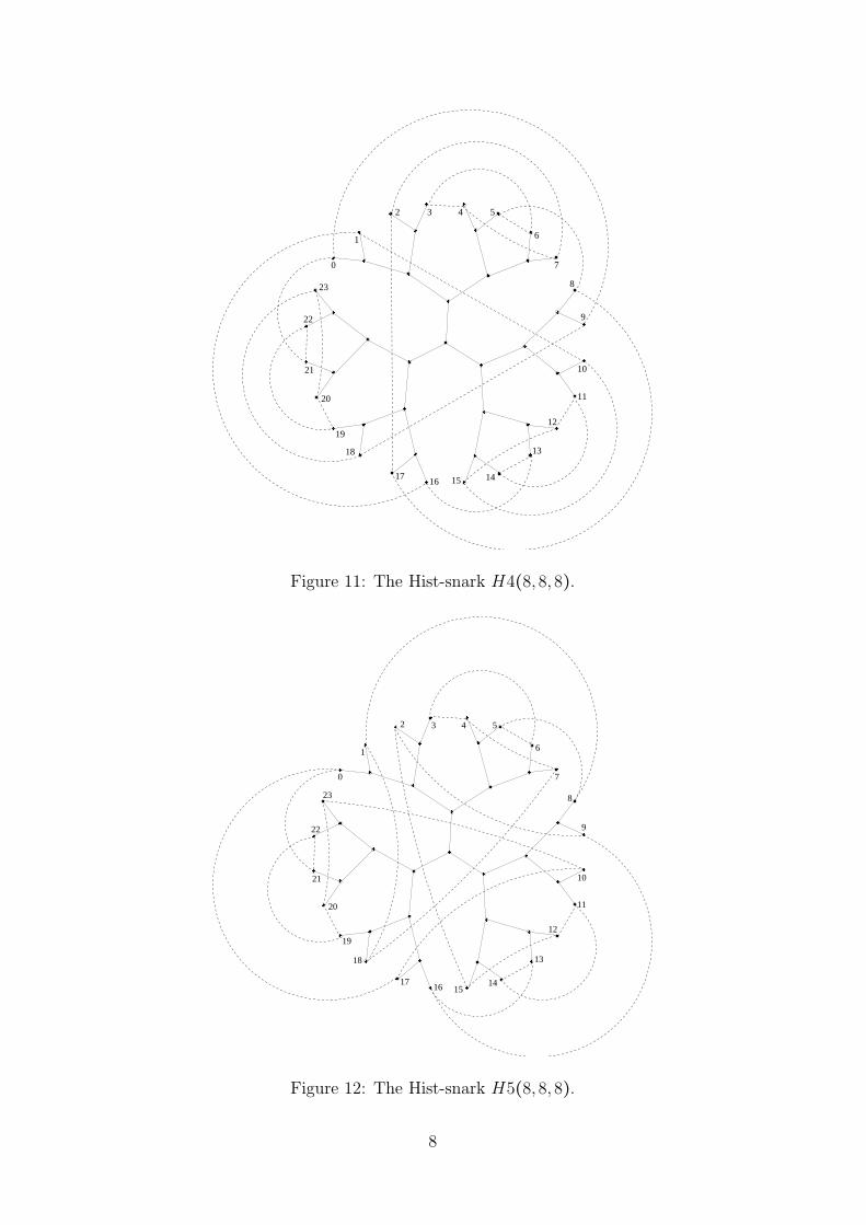
Figure 11: The Hist-snark H4(8,8,8).
����
��������
��������
����
������
������
��������
����
���
���
������
������
��������
����
������
������
��������
����
��������
��������
����
��������
��������
����
��������
����
���
���
����
����
����
��������
��������
��������
��������
��������
������
������
������
������
��������
������
������
��������
��������
����
����
����
��������
��������
��������
��������
��������
����
1
22
5
12
20
21
1716 14
19
2
6
7
9
10
11
0
8
15
43
23
18 13
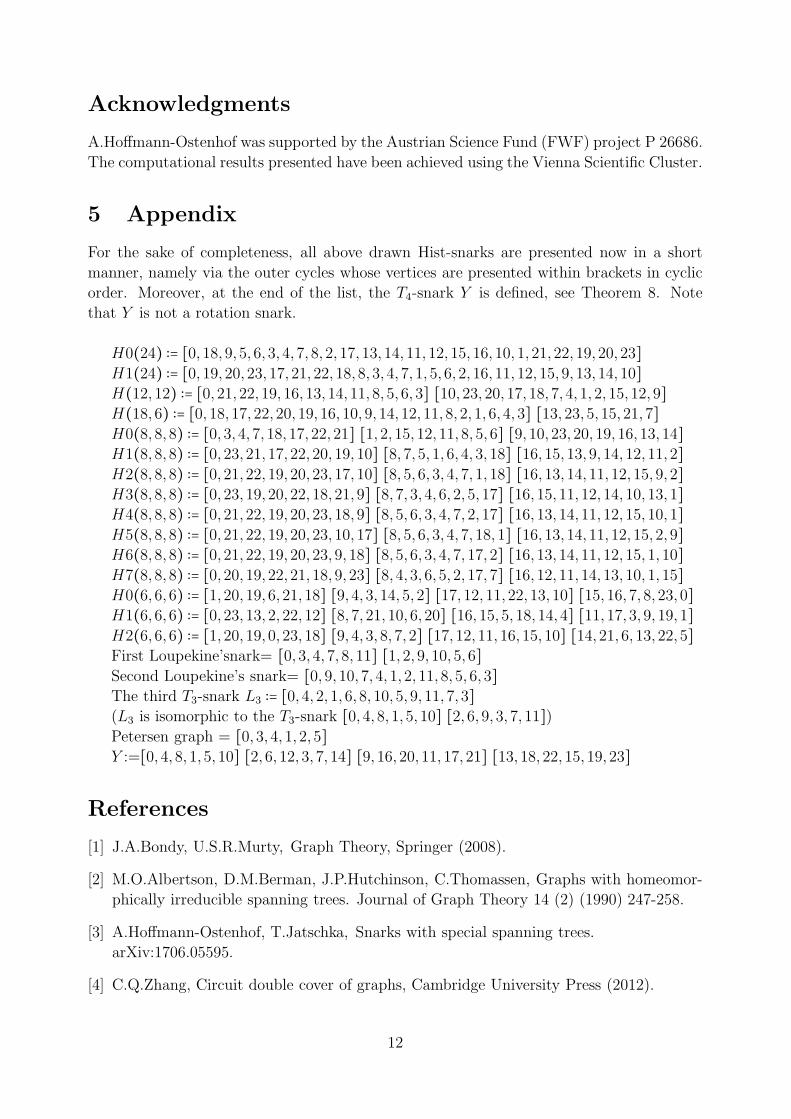
Figure 12: The Hist-snark H5(8,8,8).
8

����
����
��������
��������
����
��������
����
��������
������
������
��������
����
����
��������
���
���
���
���
��������
��������
��������
����
��������
����
��������
��������
��������
��������
������
������
��������
����
����
����
����
��������
����
��������
��������
��������
����
���
���
��������
����
������
������
��������
����
������
������
��������
������
������
22
5
13
20
21
4
14
19
2
6
9
10
11
16
8
12
7
3
1
0
23
18
17 15
Figure 13: The Hist-snark H6(8,8,8).
3 Other results on T4-snarks
Theorem 7 Let G be cyclically 4-edge connected cubic graph with girth at least 6. Then
G is 3-edge colorable if G has a spanning tree isomorphic to Ti for some i ∈ {1,2,3,4}.
Theorem 8 Let G be a T4-snark satisfying G ∈ {6,6,6,6}∗. Then the number of automor-
phisms of G is at most 128. Moreover, the T4-snark Y ∈ {6,6,6,6}∗ in the appendix below
has precisely 128 automorphisms.
4 Open problems
One motivation to consider Ti-snarks was the intention to obtain sooner or later small
snarks of girth 7 or even cyclically 7-edge connected snarks. Since the generated snarks do
not even have girth 6, we state some less ambitious open problems.
Problem 1 Is there a Ti-snark with girth k ≥ 6 for some i?
Problem 2 Is there a cyclically k-edge connected Ti-snark with k ≥ 6 for some i?
Problem 3 Is there a cyclically k-edge connected rotation Ti-snark with k ≥ 6 for some i?
Conjecture 9 There are infinitely many rotation snarks.
9

����
����
��������
��������
������
������
��������
��������
���
���
������
������
����
����
��������
����
���
���
��������
������
������
����
��������
������
������
��������
��������
������
������
��������
��������
��������
����
��������
����
����
��������
����
����
����
����
��������
��������
��������
��������
����
����
����
��������
����
��������
����
��������
1
22
12
18
4
14
19
2 3
6
9
10
11
0
23
21
20
17
8
7
5
16 15
13
Figure 14: The Hist-snark H7(8,8,8).
���
���
����
��������
��������
��������
��������
��������
����
��������
��������
����
��������
��������
����
��������
��������
��������
��������
������
������
��������
��������
��������
������
������
��������
������
������
������
������
��������
������
������
��������
��������
��������
��������
����
����
��������
��������
����
����
��������
��������
��������
����
��������
��������
����
����
1
22
12
14
19
9
20
21
23
0
23
4
5
6
7
8
10
11
13
151617
18
Figure 15: The Hist-snark H0(6,6,6,6).
10

��������
��������
����
����
������
������
����
��������
���
���
���
���
��������
��������
��������
��������
������
������
��������
���
���
����
��������
����
����
���
���
����
����
����
����
��������
��������
��������
��������
����
��������
����
��������
��������
��������
����
��������
��������
����
��������
����
��������
����
����
���
���
��������
1
23
17
23 4
5
6
7
8
9
10
11
12
13
141516
1819
20
21
22
0
Figure 16: The Hist-snark H1(6,6,6,6).
������
������
��������
����
��������
����
����
����
��������
����
����
��������
����
����
��������
��������
����
����
����
����
����
����
����
���
���
�����
���
���
���
����
���
���
����
����
��������
����
��������
������
������
��������
����
����
��������
��������
����
����
���
���
��������
����
����
����
1 6
9
21
5
0
2 3 4
7
8
10
11
13
14151617
18
19
20
22
23
12
Figure 17: The Hist-snark H2(6,6,6,6).
11
Acknowledgments
A.Hoffmann-Ostenhof was supported by the Austrian Science Fund (FWF) project P 26686.
The computational results presented have been achieved using the Vienna Scientific Cluster.
5 Appendix
For the sake of completeness, all above drawn Hist-snarks are presented now in a short
manner, namely via the outer cycles whose vertices are presented within brackets in cyclic
order. Moreover, at the end of the list, the T4-snark Y is defined, see Theorem 8. Note
that Y is not a rotation snark.
H0(24) ∶= [0,18,9,5,6,3,4,7,8,2,17,13,14,11,12,15,16,10,1,21,22,19,20,23]
H1(24) ∶= [0,19,20,23,17,21,22,18,8,3,4,7,1,5,6,2,16,11,12,15,9,13,14,10]
H(12,12) ∶= [0,21,22,19,16,13,14,11,8,5,6,3] [10,23,20,17,18,7,4,1,2,15,12,9]
H(18,6) ∶= [0,18,17,22,20,19,16,10,9,14,12,11,8,2,1,6,4,3] [13,23,5,15,21,7]
H0(8,8,8) ∶= [0,3,4,7,18,17,22,21] [1,2,15,12,11,8,5,6] [9,10,23,20,19,16,13,14]
H1(8,8,8) ∶= [0,23,21,17,22,20,19,10] [8,7,5,1,6,4,3,18] [16,15,13,9,14,12,11,2]
H2(8,8,8) ∶= [0,21,22,19,20,23,17,10] [8,5,6,3,4,7,1,18] [16,13,14,11,12,15,9,2]
H3(8,8,8) ∶= [0,23,19,20,22,18,21,9] [8,7,3,4,6,2,5,17] [16,15,11,12,14,10,13,1]
H4(8,8,8) ∶= [0,21,22,19,20,23,18,9] [8,5,6,3,4,7,2,17] [16,13,14,11,12,15,10,1]
H5(8,8,8) ∶= [0,21,22,19,20,23,10,17] [8,5,6,3,4,7,18,1] [16,13,14,11,12,15,2,9]
H6(8,8,8) ∶= [0,21,22,19,20,23,9,18] [8,5,6,3,4,7,17,2] [16,13,14,11,12,15,1,10]
H7(8,8,8) ∶= [0,20,19,22,21,18,9,23] [8,4,3,6,5,2,17,7] [16,12,11,14,13,10,1,15]
H0(6,6,6) ∶= [1,20,19,6,21,18] [9,4,3,14,5,2] [17,12,11,22,13,10] [15,16,7,8,23,0]
H1(6,6,6) ∶= [0,23,13,2,22,12] [8,7,21,10,6,20] [16,15,5,18,14,4] [11,17,3,9,19,1]
H2(6,6,6) ∶= [1,20,19,0,23,18] [9,4,3,8,7,2] [17,12,11,16,15,10] [14,21,6,13,22,5]
First Loupekine’snark= [0,3,4,7,8,11] [1,2,9,10,5,6]
Second Loupekine’s snark= [0,9,10,7,4,1,2,11,8,5,6,3]
The third T3-snark L3 ∶= [0,4,2,1,6,8,10,5,9,11,7,3]
(L3 is isomorphic to the T3-snark [0,4,8,1,5,10] [2,6,9,3,7,11])
Petersen graph = [0,3,4,1,2,5]
Y :=[0,4,8,1,5,10] [2,6,12,3,7,14] [9,16,20,11,17,21] [13,18,22,15,19,23]
References
[1] J.A.Bondy, U.S.R.Murty, Graph Theory, Springer (2008).
[2] M.O.Albertson, D.M.Berman, J.P.Hutchinson, C.Thomassen, Graphs with homeomor-
phically irreducible spanning trees. Journal of Graph Theory 14 (2) (1990) 247-258.
[3] A.Hoffmann-Ostenhof, T.Jatschka, Snarks with special spanning trees.
arXiv:1706.05595.
[4] C.Q.Zhang, Circuit double cover of graphs, Cambridge University Press (2012).
12