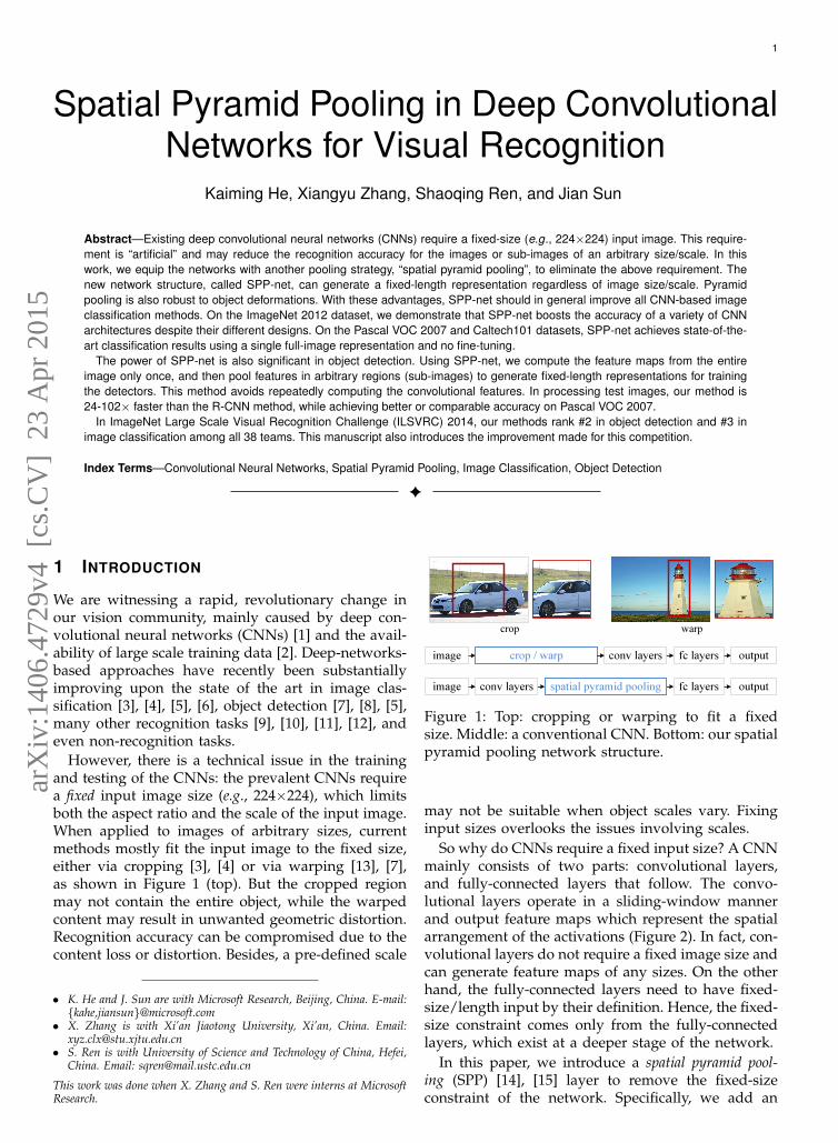
1

Spatial Pyramid Pooling in Deep ConvolutionalNetworks for Visual Recognition

Kaiming He, Xiangyu Zhang, Shaoqing Ren, and Jian Sun

Abstract—Existing deep convolutional neural networks (CNNs) require a fixed-size (e.g., 224×224) input image. This require-ment is “artificial” and may reduce the recognition accuracy for the images or sub-images of an arbitrary size/scale. In thiswork, we equip the networks with another pooling strategy, “spatial pyramid pooling”, to eliminate the above requirement. Thenew network structure, called SPP-net, can generate a fixed-length representation regardless of image size/scale. Pyramidpooling is also robust to object deformations. With these advantages, SPP-net should in general improve all CNN-based imageclassification methods. On the ImageNet 2012 dataset, we demonstrate that SPP-net boosts the accuracy of a variety of CNNarchitectures despite their different designs. On the Pascal VOC 2007 and Caltech101 datasets, SPP-net achieves state-of-the-art classification results using a single full-image representation and no fine-tuning.

The power of SPP-net is also significant in object detection. Using SPP-net, we compute the feature maps from the entireimage only once, and then pool features in arbitrary regions (sub-images) to generate fixed-length representations for trainingthe detectors. This method avoids repeatedly computing the convolutional features. In processing test images, our method is24-102× faster than the R-CNN method, while achieving better or comparable accuracy on Pascal VOC 2007.

In ImageNet Large Scale Visual Recognition Challenge (ILSVRC) 2014, our methods rank #2 in object detection and #3 inimage classification among all 38 teams. This manuscript also introduces the improvement made for this competition.

Index Terms—Convolutional Neural Networks, Spatial Pyramid Pooling, Image Classification, Object Detection

F

1 INTRODUCTION

We are witnessing a rapid, revolutionary change inour vision community, mainly caused by deep con-volutional neural networks (CNNs) [1] and the avail-ability of large scale training data [2]. Deep-networks-based approaches have recently been substantiallyimproving upon the state of the art in image clas-sification [3], [4], [5], [6], object detection [7], [8], [5],many other recognition tasks [9], [10], [11], [12], andeven non-recognition tasks.

However, there is a technical issue in the trainingand testing of the CNNs: the prevalent CNNs requirea fixed input image size (e.g., 224×224), which limitsboth the aspect ratio and the scale of the input image.When applied to images of arbitrary sizes, currentmethods mostly fit the input image to the fixed size,either via cropping [3], [4] or via warping [13], [7],as shown in Figure 1 (top). But the cropped regionmay not contain the entire object, while the warpedcontent may result in unwanted geometric distortion.Recognition accuracy can be compromised due to thecontent loss or distortion. Besides, a pre-defined scale

• K. He and J. Sun are with Microsoft Research, Beijing, China. E-mail:{kahe,jiansun}@microsoft.com

• X. Zhang is with Xi’an Jiaotong University, Xi’an, China. Email:xyz.clx@stu.xjtu.edu.cn

• S. Ren is with University of Science and Technology of China, Hefei,China. Email: sqren@mail.ustc.edu.cn

This work was done when X. Zhang and S. Ren were interns at MicrosoftResearch.

crop warp

spatial pyramid pooling

crop / warp

conv layersimage fc layers output

image conv layers fc layers output

Figure 1: Top: cropping or warping to fit a fixedsize. Middle: a conventional CNN. Bottom: our spatialpyramid pooling network structure.

may not be suitable when object scales vary. Fixinginput sizes overlooks the issues involving scales.

So why do CNNs require a fixed input size? A CNNmainly consists of two parts: convolutional layers,and fully-connected layers that follow. The convo-lutional layers operate in a sliding-window mannerand output feature maps which represent the spatialarrangement of the activations (Figure 2). In fact, con-volutional layers do not require a fixed image size andcan generate feature maps of any sizes. On the otherhand, the fully-connected layers need to have fixed-size/length input by their definition. Hence, the fixed-size constraint comes only from the fully-connectedlayers, which exist at a deeper stage of the network.

In this paper, we introduce a spatial pyramid pool-ing (SPP) [14], [15] layer to remove the fixed-sizeconstraint of the network. Specifically, we add an

arX

iv:1

406.

4729

v4 [

cs.C

V]

23

Apr

201

5

2

SPP layer on top of the last convolutional layer. TheSPP layer pools the features and generates fixed-length outputs, which are then fed into the fully-connected layers (or other classifiers). In other words,we perform some information “aggregation” at adeeper stage of the network hierarchy (between con-volutional layers and fully-connected layers) to avoidthe need for cropping or warping at the beginning.Figure 1 (bottom) shows the change of the networkarchitecture by introducing the SPP layer. We call thenew network structure SPP-net.

Spatial pyramid pooling [14], [15] (popularlyknown as spatial pyramid matching or SPM [15]), asan extension of the Bag-of-Words (BoW) model [16],is one of the most successful methods in computervision. It partitions the image into divisions fromfiner to coarser levels, and aggregates local featuresin them. SPP has long been a key component in theleading and competition-winning systems for classi-fication (e.g., [17], [18], [19]) and detection (e.g., [20])before the recent prevalence of CNNs. Nevertheless,SPP has not been considered in the context of CNNs.We note that SPP has several remarkable propertiesfor deep CNNs: 1) SPP is able to generate a fixed-length output regardless of the input size, while thesliding window pooling used in the previous deepnetworks [3] cannot; 2) SPP uses multi-level spatialbins, while the sliding window pooling uses onlya single window size. Multi-level pooling has beenshown to be robust to object deformations [15]; 3) SPPcan pool features extracted at variable scales thanksto the flexibility of input scales. Through experimentswe show that all these factors elevate the recognitionaccuracy of deep networks.

SPP-net not only makes it possible to generate rep-resentations from arbitrarily sized images/windowsfor testing, but also allows us to feed images withvarying sizes or scales during training. Training withvariable-size images increases scale-invariance andreduces over-fitting. We develop a simple multi-sizetraining method. For a single network to acceptvariable input sizes, we approximate it by multiplenetworks that share all parameters, while each ofthese networks is trained using a fixed input size. Ineach epoch we train the network with a given inputsize, and switch to another input size for the nextepoch. Experiments show that this multi-size trainingconverges just as the traditional single-size training,and leads to better testing accuracy.

The advantages of SPP are orthogonal to the specificCNN designs. In a series of controlled experiments onthe ImageNet 2012 dataset, we demonstrate that SPPimproves four different CNN architectures in existingpublications [3], [4], [5] (or their modifications), overthe no-SPP counterparts. These architectures havevarious filter numbers/sizes, strides, depths, or otherdesigns. It is thus reasonable for us to conjecturethat SPP should improve more sophisticated (deeper

and larger) convolutional architectures. SPP-net alsoshows state-of-the-art classification results on Cal-tech101 [21] and Pascal VOC 2007 [22] using only asingle full-image representation and no fine-tuning.

SPP-net also shows great strength in object detec-tion. In the leading object detection method R-CNN[7], the features from candidate windows are extractedvia deep convolutional networks. This method showsremarkable detection accuracy on both the VOC andImageNet datasets. But the feature computation in R-CNN is time-consuming, because it repeatedly appliesthe deep convolutional networks to the raw pixelsof thousands of warped regions per image. In thispaper, we show that we can run the convolutionallayers only once on the entire image (regardless ofthe number of windows), and then extract featuresby SPP-net on the feature maps. This method yieldsa speedup of over one hundred times over R-CNN.Note that training/running a detector on the featuremaps (rather than image regions) is actually a morepopular idea [23], [24], [20], [5]. But SPP-net inheritsthe power of the deep CNN feature maps and also theflexibility of SPP on arbitrary window sizes, whichleads to outstanding accuracy and efficiency. In ourexperiment, the SPP-net-based system (built upon theR-CNN pipeline) computes features 24-102× fasterthan R-CNN, while has better or comparable accuracy.With the recent fast proposal method of EdgeBoxes[25], our system takes 0.5 seconds processing an image(including all steps). This makes our method practicalfor real-world applications.

A preliminary version of this manuscript has beenpublished in ECCV 2014. Based on this work, weattended the competition of ILSVRC 2014 [26], andranked #2 in object detection and #3 in image clas-sification (both are provided-data-only tracks) amongall 38 teams. There are a few modifications madefor ILSVRC 2014. We show that the SPP-nets canboost various networks that are deeper and larger(Sec. 3.1.2-3.1.4) over the no-SPP counterparts. Fur-ther, driven by our detection framework, we findthat multi-view testing on feature maps with flexiblylocated/sized windows (Sec. 3.1.5) can increase theclassification accuracy. This manuscript also providesthe details of these modifications.

We have released the code to facilitate future re-search (http://research.microsoft.com/en-us/um/people/kahe/).

2 DEEP NETWORKS WITH SPATIAL PYRA-MID POOLING

2.1 Convolutional Layers and Feature Maps

Consider the popular seven-layer architectures [3], [4].The first five layers are convolutional, some of whichare followed by pooling layers. These pooling layerscan also be considered as “convolutional”, in the sensethat they are using sliding windows. The last two

3

filter #175

filter #55

(a) image (b) feature maps (c) strongest activations

filter #66

filter #118

(a) image (b) feature maps (c) strongest activations

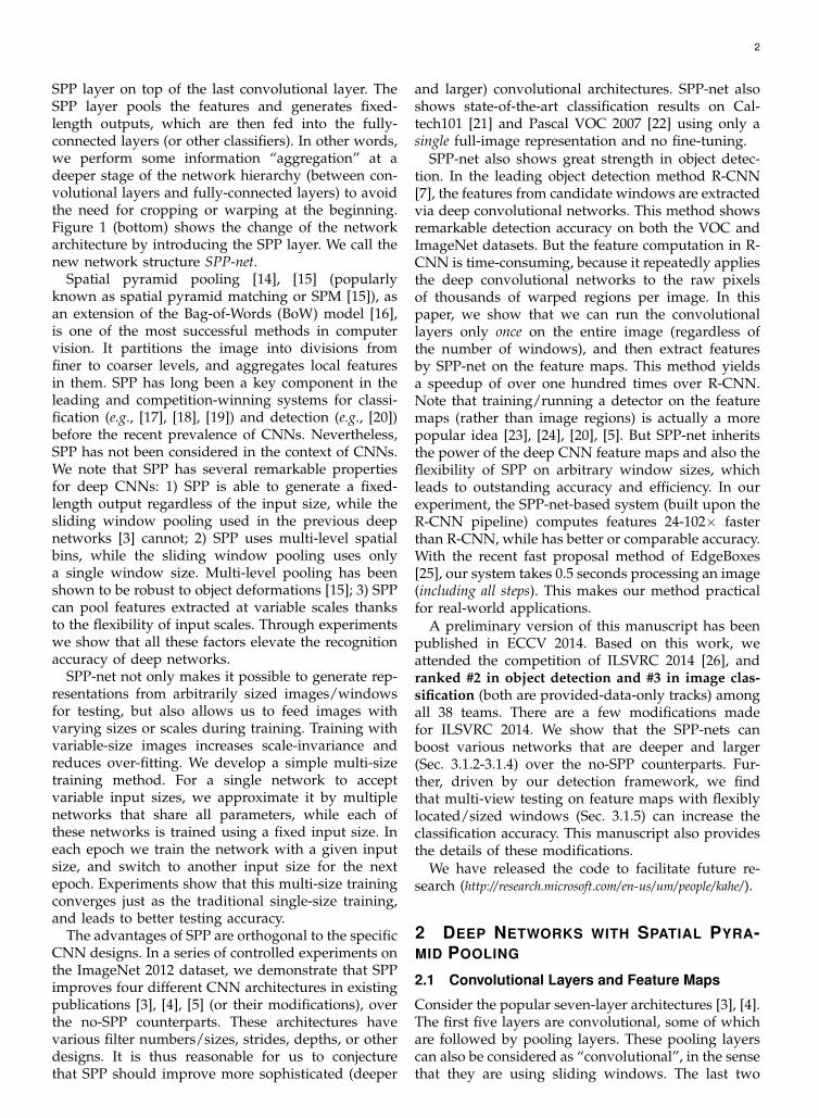
Figure 2: Visualization of the feature maps. (a) Two images in Pascal VOC 2007. (b) The feature maps of someconv5 filters. The arrows indicate the strongest responses and their corresponding positions in the images.(c) The ImageNet images that have the strongest responses of the corresponding filters. The green rectanglesmark the receptive fields of the strongest responses.

layers are fully connected, with an N-way softmax asthe output, where N is the number of categories.

The deep network described above needs a fixedimage size. However, we notice that the requirementof fixed sizes is only due to the fully-connected layersthat demand fixed-length vectors as inputs. On theother hand, the convolutional layers accept inputs ofarbitrary sizes. The convolutional layers use slidingfilters, and their outputs have roughly the same aspectratio as the inputs. These outputs are known as featuremaps [1] - they involve not only the strength of theresponses, but also their spatial positions.

In Figure 2, we visualize some feature maps. Theyare generated by some filters of the conv5 layer. Fig-ure 2(c) shows the strongest activated images of thesefilters in the ImageNet dataset. We see a filter can beactivated by some semantic content. For example, the55-th filter (Figure 2, bottom left) is most activated bya circle shape; the 66-th filter (Figure 2, top right) ismost activated by a ∧-shape; and the 118-th filter (Fig-ure 2, bottom right) is most activated by a ∨-shape.These shapes in the input images (Figure 2(a)) activatethe feature maps at the corresponding positions (thearrows in Figure 2).

It is worth noticing that we generate the featuremaps in Figure 2 without fixing the input size. Thesefeature maps generated by deep convolutional lay-ers are analogous to the feature maps in traditionalmethods [27], [28]. In those methods, SIFT vectors[29] or image patches [28] are densely extracted andthen encoded, e.g., by vector quantization [16], [15],[30], sparse coding [17], [18], or Fisher kernels [19].These encoded features consist of the feature maps,and are then pooled by Bag-of-Words (BoW) [16] orspatial pyramids [14], [15]. Analogously, the deepconvolutional features can be pooled in a similar way.

2.2 The Spatial Pyramid Pooling LayerThe convolutional layers accept arbitrary input sizes,but they produce outputs of variable sizes. The classi-fiers (SVM/softmax) or fully-connected layers require

convolutional layers

feature maps of conv5

(arbitrary size)

fixed-length representation

input image

16×256-d 4×256-d 256-d

…...

…...

spatial pyramid pooling layer

fully-connected layers (fc6, fc7)

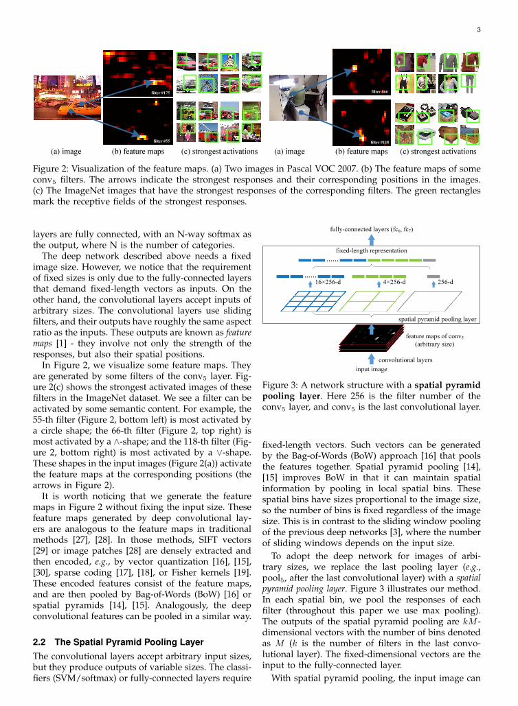
Figure 3: A network structure with a spatial pyramidpooling layer. Here 256 is the filter number of theconv5 layer, and conv5 is the last convolutional layer.

fixed-length vectors. Such vectors can be generatedby the Bag-of-Words (BoW) approach [16] that poolsthe features together. Spatial pyramid pooling [14],[15] improves BoW in that it can maintain spatialinformation by pooling in local spatial bins. Thesespatial bins have sizes proportional to the image size,so the number of bins is fixed regardless of the imagesize. This is in contrast to the sliding window poolingof the previous deep networks [3], where the numberof sliding windows depends on the input size.

To adopt the deep network for images of arbi-trary sizes, we replace the last pooling layer (e.g.,pool5, after the last convolutional layer) with a spatialpyramid pooling layer. Figure 3 illustrates our method.In each spatial bin, we pool the responses of eachfilter (throughout this paper we use max pooling).The outputs of the spatial pyramid pooling are kM -dimensional vectors with the number of bins denotedas M (k is the number of filters in the last convo-lutional layer). The fixed-dimensional vectors are theinput to the fully-connected layer.

With spatial pyramid pooling, the input image can

4

be of any sizes. This not only allows arbitrary aspectratios, but also allows arbitrary scales. We can resizethe input image to any scale (e.g., min(w, h)=180, 224,...) and apply the same deep network. When theinput image is at different scales, the network (withthe same filter sizes) will extract features at differentscales. The scales play important roles in traditionalmethods, e.g., the SIFT vectors are often extracted atmultiple scales [29], [27] (determined by the sizes ofthe patches and Gaussian filters). We will show thatthe scales are also important for the accuracy of deepnetworks.

Interestingly, the coarsest pyramid level has a singlebin that covers the entire image. This is in fact a“global pooling” operation, which is also investigatedin several concurrent works. In [31], [32] a globalaverage pooling is used to reduce the model sizeand also reduce overfitting; in [33], a global averagepooling is used on the testing stage after all fc layersto improve accuracy; in [34], a global max pooling isused for weakly supervised object recognition. Theglobal pooling operation corresponds to the tradi-tional Bag-of-Words method.

2.3 Training the NetworkTheoretically, the above network structure can betrained with standard back-propagation [1], regard-less of the input image size. But in practice the GPUimplementations (such as cuda-convnet [3] and Caffe[35]) are preferably run on fixed input images. Nextwe describe our training solution that takes advantageof these GPU implementations while still preservingthe spatial pyramid pooling behaviors.

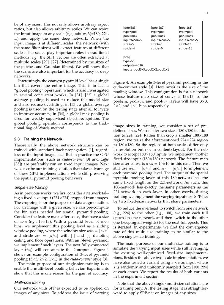
Single-size trainingAs in previous works, we first consider a network tak-ing a fixed-size input (224×224) cropped from images.The cropping is for the purpose of data augmentation.For an image with a given size, we can pre-computethe bin sizes needed for spatial pyramid pooling.Consider the feature maps after conv5 that have a sizeof a×a (e.g., 13×13). With a pyramid level of n×nbins, we implement this pooling level as a slidingwindow pooling, where the window size win = da/neand stride str = ba/nc with d·e and b·c denotingceiling and floor operations. With an l-level pyramid,we implement l such layers. The next fully-connectedlayer (fc6) will concatenate the l outputs. Figure 4shows an example configuration of 3-level pyramidpooling (3×3, 2×2, 1×1) in the cuda-convnet style [3].

The main purpose of our single-size training is toenable the multi-level pooling behavior. Experimentsshow that this is one reason for the gain of accuracy.

Multi-size trainingOur network with SPP is expected to be applied onimages of any sizes. To address the issue of varying

[fc6]

type=fc

outputs=4096

inputs=pool3x3,pool2x2,pool1x1

[pool1x1]

type=pool

pool=max

inputs=conv5

sizeX=13

stride=13

[pool3x3]

type=pool

pool=max

inputs=conv5

sizeX=5

stride=4

[pool2x2]

type=pool

pool=max

inputs=conv5

sizeX=7

stride=6

Figure 4: An example 3-level pyramid pooling in thecuda-convnet style [3]. Here sizeX is the size of thepooling window. This configuration is for a networkwhose feature map size of conv5 is 13×13, so thepool3×3, pool2×2, and pool1×1 layers will have 3×3,2×2, and 1×1 bins respectively.

image sizes in training, we consider a set of pre-defined sizes. We consider two sizes: 180×180 in addi-tion to 224×224. Rather than crop a smaller 180×180region, we resize the aforementioned 224×224 regionto 180×180. So the regions at both scales differ onlyin resolution but not in content/layout. For the net-work to accept 180×180 inputs, we implement anotherfixed-size-input (180×180) network. The feature mapsize after conv5 is a×a = 10×10 in this case. Then westill use win = da/ne and str = ba/nc to implementeach pyramid pooling level. The output of the spatialpyramid pooling layer of this 180-network has thesame fixed length as the 224-network. As such, this180-network has exactly the same parameters as the224-network in each layer. In other words, duringtraining we implement the varying-input-size SPP-netby two fixed-size networks that share parameters.

To reduce the overhead to switch from one network(e.g., 224) to the other (e.g., 180), we train each fullepoch on one network, and then switch to the otherone (keeping all weights) for the next full epoch. Thisis iterated. In experiments, we find the convergencerate of this multi-size training to be similar to theabove single-size training.

The main purpose of our multi-size training is tosimulate the varying input sizes while still leveragingthe existing well-optimized fixed-size implementa-tions. Besides the above two-scale implementation, wehave also tested a variant using s× s as input wheres is randomly and uniformly sampled from [180, 224]at each epoch. We report the results of both variantsin the experiment section.

Note that the above single/multi-size solutions arefor training only. At the testing stage, it is straightfor-ward to apply SPP-net on images of any sizes.

5

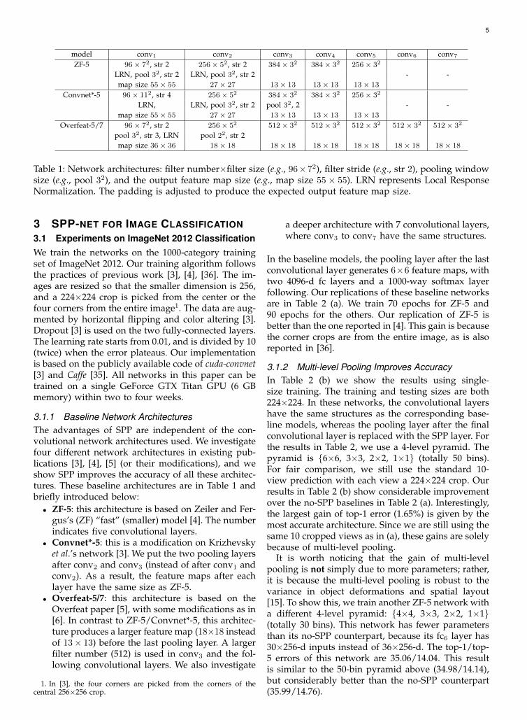
model conv1 conv2 conv3 conv4 conv5 conv6 conv7

ZF-5 96× 72, str 2 256× 52, str 2 384× 32 384× 32 256× 32

LRN, pool 32, str 2 LRN, pool 32, str 2 - -map size 55× 55 27× 27 13× 13 13× 13 13× 13

Convnet*-5 96× 112, str 4 256× 52 384× 32 384× 32 256× 32

LRN, LRN, pool 32, str 2 pool 32, 2 - -map size 55× 55 27× 27 13× 13 13× 13 13× 13

Overfeat-5/7 96× 72, str 2 256× 52 512× 32 512× 32 512× 32 512× 32 512× 32

pool 32, str 3, LRN pool 22, str 2map size 36× 36 18× 18 18× 18 18× 18 18× 18 18× 18 18× 18

Table 1: Network architectures: filter number×filter size (e.g., 96×72), filter stride (e.g., str 2), pooling windowsize (e.g., pool 32), and the output feature map size (e.g., map size 55 × 55). LRN represents Local ResponseNormalization. The padding is adjusted to produce the expected output feature map size.

3 SPP-NET FOR IMAGE CLASSIFICATION3.1 Experiments on ImageNet 2012 ClassificationWe train the networks on the 1000-category trainingset of ImageNet 2012. Our training algorithm followsthe practices of previous work [3], [4], [36]. The im-ages are resized so that the smaller dimension is 256,and a 224×224 crop is picked from the center or thefour corners from the entire image1. The data are aug-mented by horizontal flipping and color altering [3].Dropout [3] is used on the two fully-connected layers.The learning rate starts from 0.01, and is divided by 10(twice) when the error plateaus. Our implementationis based on the publicly available code of cuda-convnet[3] and Caffe [35]. All networks in this paper can betrained on a single GeForce GTX Titan GPU (6 GBmemory) within two to four weeks.

3.1.1 Baseline Network ArchitecturesThe advantages of SPP are independent of the con-volutional network architectures used. We investigatefour different network architectures in existing pub-lications [3], [4], [5] (or their modifications), and weshow SPP improves the accuracy of all these architec-tures. These baseline architectures are in Table 1 andbriefly introduced below:• ZF-5: this architecture is based on Zeiler and Fer-

gus’s (ZF) “fast” (smaller) model [4]. The numberindicates five convolutional layers.

• Convnet*-5: this is a modification on Krizhevskyet al.’s network [3]. We put the two pooling layersafter conv2 and conv3 (instead of after conv1 andconv2). As a result, the feature maps after eachlayer have the same size as ZF-5.

• Overfeat-5/7: this architecture is based on theOverfeat paper [5], with some modifications as in[6]. In contrast to ZF-5/Convnet*-5, this architec-ture produces a larger feature map (18×18 insteadof 13× 13) before the last pooling layer. A largerfilter number (512) is used in conv3 and the fol-lowing convolutional layers. We also investigate

1. In [3], the four corners are picked from the corners of thecentral 256×256 crop.

a deeper architecture with 7 convolutional layers,where conv3 to conv7 have the same structures.

In the baseline models, the pooling layer after the lastconvolutional layer generates 6×6 feature maps, withtwo 4096-d fc layers and a 1000-way softmax layerfollowing. Our replications of these baseline networksare in Table 2 (a). We train 70 epochs for ZF-5 and90 epochs for the others. Our replication of ZF-5 isbetter than the one reported in [4]. This gain is becausethe corner crops are from the entire image, as is alsoreported in [36].

3.1.2 Multi-level Pooling Improves AccuracyIn Table 2 (b) we show the results using single-size training. The training and testing sizes are both224×224. In these networks, the convolutional layershave the same structures as the corresponding base-line models, whereas the pooling layer after the finalconvolutional layer is replaced with the SPP layer. Forthe results in Table 2, we use a 4-level pyramid. Thepyramid is {6×6, 3×3, 2×2, 1×1} (totally 50 bins).For fair comparison, we still use the standard 10-view prediction with each view a 224×224 crop. Ourresults in Table 2 (b) show considerable improvementover the no-SPP baselines in Table 2 (a). Interestingly,the largest gain of top-1 error (1.65%) is given by themost accurate architecture. Since we are still using thesame 10 cropped views as in (a), these gains are solelybecause of multi-level pooling.

It is worth noticing that the gain of multi-levelpooling is not simply due to more parameters; rather,it is because the multi-level pooling is robust to thevariance in object deformations and spatial layout[15]. To show this, we train another ZF-5 network witha different 4-level pyramid: {4×4, 3×3, 2×2, 1×1}(totally 30 bins). This network has fewer parametersthan its no-SPP counterpart, because its fc6 layer has30×256-d inputs instead of 36×256-d. The top-1/top-5 errors of this network are 35.06/14.04. This resultis similar to the 50-bin pyramid above (34.98/14.14),but considerably better than the no-SPP counterpart(35.99/14.76).

6

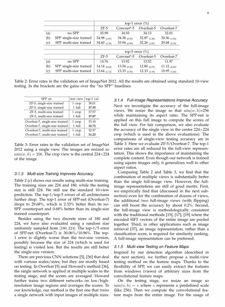
top-1 error (%)ZF-5 Convnet*-5 Overfeat-5 Overfeat-7

(a) no SPP 35.99 34.93 34.13 32.01(b) SPP single-size trained 34.98 (1.01) 34.38 (0.55) 32.87 (1.26) 30.36 (1.65)

(c) SPP multi-size trained 34.60 (1.39) 33.94 (0.99) 32.26 (1.87) 29.68 (2.33)

top-5 error (%)ZF-5 Convnet*-5 Overfeat-5 Overfeat-7

(a) no SPP 14.76 13.92 13.52 11.97(b) SPP single-size trained 14.14 (0.62) 13.54 (0.38) 12.80 (0.72) 11.12 (0.85)

(c) SPP multi-size trained 13.64 (1.12) 13.33 (0.59) 12.33 (1.19) 10.95 (1.02)

Table 2: Error rates in the validation set of ImageNet 2012. All the results are obtained using standard 10-viewtesting. In the brackets are the gains over the “no SPP” baselines.

SPP on test view top-1 valZF-5, single-size trained 1 crop 38.01ZF-5, single-size trained 1 full 37.55ZF-5, multi-size trained 1 crop 37.57ZF-5, multi-size trained 1 full 37.07

Overfeat-7, single-size trained 1 crop 33.18Overfeat-7, single-size trained 1 full 32.72Overfeat-7, multi-size trained 1 crop 32.57Overfeat-7, multi-size trained 1 full 31.25

Table 3: Error rates in the validation set of ImageNet2012 using a single view. The images are resized somin(w, h) = 256. The crop view is the central 224×224of the image.

3.1.3 Multi-size Training Improves Accuracy

Table 2 (c) shows our results using multi-size training.The training sizes are 224 and 180, while the testingsize is still 224. We still use the standard 10-viewprediction. The top-1/top-5 errors of all architecturesfurther drop. The top-1 error of SPP-net (Overfeat-7)drops to 29.68%, which is 2.33% better than its no-SPP counterpart and 0.68% better than its single-sizetrained counterpart.

Besides using the two discrete sizes of 180 and224, we have also evaluated using a random sizeuniformly sampled from [180, 224]. The top-1/5 errorof SPP-net (Overfeat-7) is 30.06%/10.96%. The top-1 error is slightly worse than the two-size version,possibly because the size of 224 (which is used fortesting) is visited less. But the results are still betterthe single-size version.

There are previous CNN solutions [5], [36] that dealwith various scales/sizes, but they are mostly basedon testing. In Overfeat [5] and Howard’s method [36],the single network is applied at multiple scales in thetesting stage, and the scores are averaged. Howardfurther trains two different networks on low/high-resolution image regions and averages the scores. Toour knowledge, our method is the first one that trainsa single network with input images of multiple sizes.

3.1.4 Full-image Representations Improve AccuracyNext we investigate the accuracy of the full-imageviews. We resize the image so that min(w, h)=256while maintaining its aspect ratio. The SPP-net isapplied on this full image to compute the scores ofthe full view. For fair comparison, we also evaluatethe accuracy of the single view in the center 224×224crop (which is used in the above evaluations). Thecomparisons of single-view testing accuracy are inTable 3. Here we evaluate ZF-5/Overfeat-7. The top-1error rates are all reduced by the full-view represen-tation. This shows the importance of maintaining thecomplete content. Even though our network is trainedusing square images only, it generalizes well to otheraspect ratios.

Comparing Table 2 and Table 3, we find that thecombination of multiple views is substantially betterthan the single full-image view. However, the full-image representations are still of good merits. First,we empirically find that (discussed in the next sub-section) even for the combination of dozens of views,the additional two full-image views (with flipping)can still boost the accuracy by about 0.2%. Second,the full-image view is methodologically consistentwith the traditional methods [15], [17], [19] where theencoded SIFT vectors of the entire image are pooledtogether. Third, in other applications such as imageretrieval [37], an image representation, rather than aclassification score, is required for similarity ranking.A full-image representation can be preferred.

3.1.5 Multi-view Testing on Feature MapsInspired by our detection algorithm (described inthe next section), we further propose a multi-viewtesting method on the feature maps. Thanks to theflexibility of SPP, we can easily extract the featuresfrom windows (views) of arbitrary sizes from theconvolutional feature maps.

On the testing stage, we resize an image somin(w, h) = s where s represents a predefined scale(like 256). Then we compute the convolutional fea-ture maps from the entire image. For the usage of

7

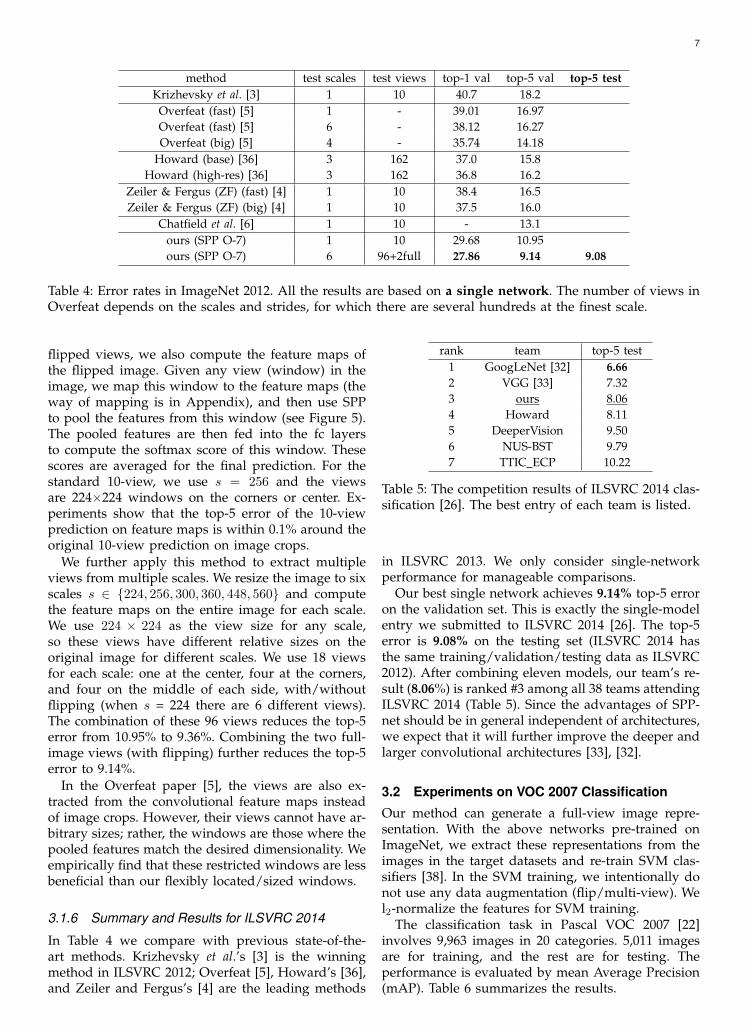
method test scales test views top-1 val top-5 val top-5 testKrizhevsky et al. [3] 1 10 40.7 18.2

Overfeat (fast) [5] 1 - 39.01 16.97Overfeat (fast) [5] 6 - 38.12 16.27Overfeat (big) [5] 4 - 35.74 14.18

Howard (base) [36] 3 162 37.0 15.8Howard (high-res) [36] 3 162 36.8 16.2

Zeiler & Fergus (ZF) (fast) [4] 1 10 38.4 16.5Zeiler & Fergus (ZF) (big) [4] 1 10 37.5 16.0

Chatfield et al. [6] 1 10 - 13.1ours (SPP O-7) 1 10 29.68 10.95ours (SPP O-7) 6 96+2full 27.86 9.14 9.08

Table 4: Error rates in ImageNet 2012. All the results are based on a single network. The number of views inOverfeat depends on the scales and strides, for which there are several hundreds at the finest scale.

flipped views, we also compute the feature maps ofthe flipped image. Given any view (window) in theimage, we map this window to the feature maps (theway of mapping is in Appendix), and then use SPPto pool the features from this window (see Figure 5).The pooled features are then fed into the fc layersto compute the softmax score of this window. Thesescores are averaged for the final prediction. For thestandard 10-view, we use s = 256 and the viewsare 224×224 windows on the corners or center. Ex-periments show that the top-5 error of the 10-viewprediction on feature maps is within 0.1% around theoriginal 10-view prediction on image crops.

We further apply this method to extract multipleviews from multiple scales. We resize the image to sixscales s ∈ {224, 256, 300, 360, 448, 560} and computethe feature maps on the entire image for each scale.We use 224 × 224 as the view size for any scale,so these views have different relative sizes on theoriginal image for different scales. We use 18 viewsfor each scale: one at the center, four at the corners,and four on the middle of each side, with/withoutflipping (when s = 224 there are 6 different views).The combination of these 96 views reduces the top-5error from 10.95% to 9.36%. Combining the two full-image views (with flipping) further reduces the top-5error to 9.14%.

In the Overfeat paper [5], the views are also ex-tracted from the convolutional feature maps insteadof image crops. However, their views cannot have ar-bitrary sizes; rather, the windows are those where thepooled features match the desired dimensionality. Weempirically find that these restricted windows are lessbeneficial than our flexibly located/sized windows.

3.1.6 Summary and Results for ILSVRC 2014

In Table 4 we compare with previous state-of-the-art methods. Krizhevsky et al.’s [3] is the winningmethod in ILSVRC 2012; Overfeat [5], Howard’s [36],and Zeiler and Fergus’s [4] are the leading methods

rank team top-5 test1 GoogLeNet [32] 6.662 VGG [33] 7.323 ours 8.064 Howard 8.115 DeeperVision 9.506 NUS-BST 9.797 TTIC ECP 10.22

Table 5: The competition results of ILSVRC 2014 clas-sification [26]. The best entry of each team is listed.

in ILSVRC 2013. We only consider single-networkperformance for manageable comparisons.

Our best single network achieves 9.14% top-5 erroron the validation set. This is exactly the single-modelentry we submitted to ILSVRC 2014 [26]. The top-5error is 9.08% on the testing set (ILSVRC 2014 hasthe same training/validation/testing data as ILSVRC2012). After combining eleven models, our team’s re-sult (8.06%) is ranked #3 among all 38 teams attendingILSVRC 2014 (Table 5). Since the advantages of SPP-net should be in general independent of architectures,we expect that it will further improve the deeper andlarger convolutional architectures [33], [32].

3.2 Experiments on VOC 2007 Classification

Our method can generate a full-view image repre-sentation. With the above networks pre-trained onImageNet, we extract these representations from theimages in the target datasets and re-train SVM clas-sifiers [38]. In the SVM training, we intentionally donot use any data augmentation (flip/multi-view). Wel2-normalize the features for SVM training.

The classification task in Pascal VOC 2007 [22]involves 9,963 images in 20 categories. 5,011 imagesare for training, and the rest are for testing. Theperformance is evaluated by mean Average Precision(mAP). Table 6 summarizes the results.

8

(a) (b) (c) (d) (e)model no SPP (ZF-5) SPP (ZF-5) SPP (ZF-5) SPP (ZF-5) SPP (Overfeat-7)

crop crop full full fullsize 224×224 224×224 224×- 392×- 364×-

conv4 59.96 57.28 - - -conv5 66.34 65.43 - - -

pool5/7 (6×6) 69.14 68.76 70.82 71.67 76.09fc6/8 74.86 75.55 77.32 78.78 81.58fc7/9 75.90 76.45 78.39 80.10 82.44

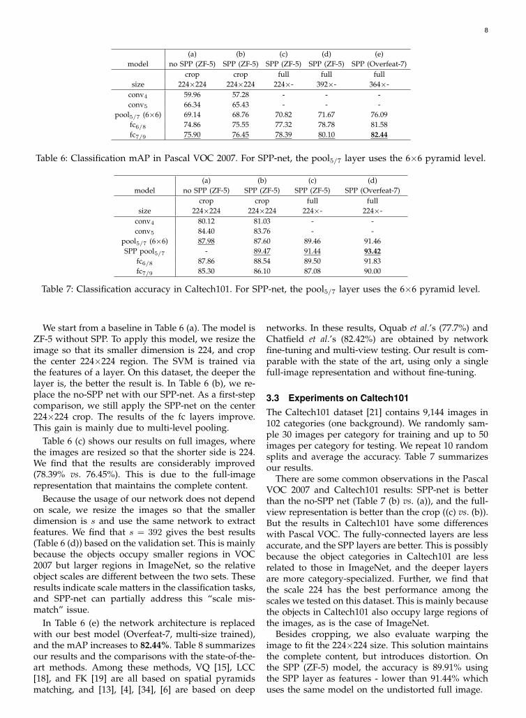
Table 6: Classification mAP in Pascal VOC 2007. For SPP-net, the pool5/7 layer uses the 6×6 pyramid level.

(a) (b) (c) (d)model no SPP (ZF-5) SPP (ZF-5) SPP (ZF-5) SPP (Overfeat-7)

crop crop full fullsize 224×224 224×224 224×- 224×-

conv4 80.12 81.03 - -conv5 84.40 83.76 - -

pool5/7 (6×6) 87.98 87.60 89.46 91.46SPP pool5/7 - 89.47 91.44 93.42

fc6/8 87.86 88.54 89.50 91.83fc7/9 85.30 86.10 87.08 90.00

Table 7: Classification accuracy in Caltech101. For SPP-net, the pool5/7 layer uses the 6×6 pyramid level.

We start from a baseline in Table 6 (a). The model isZF-5 without SPP. To apply this model, we resize theimage so that its smaller dimension is 224, and cropthe center 224×224 region. The SVM is trained viathe features of a layer. On this dataset, the deeper thelayer is, the better the result is. In Table 6 (b), we re-place the no-SPP net with our SPP-net. As a first-stepcomparison, we still apply the SPP-net on the center224×224 crop. The results of the fc layers improve.This gain is mainly due to multi-level pooling.

Table 6 (c) shows our results on full images, wherethe images are resized so that the shorter side is 224.We find that the results are considerably improved(78.39% vs. 76.45%). This is due to the full-imagerepresentation that maintains the complete content.

Because the usage of our network does not dependon scale, we resize the images so that the smallerdimension is s and use the same network to extractfeatures. We find that s = 392 gives the best results(Table 6 (d)) based on the validation set. This is mainlybecause the objects occupy smaller regions in VOC2007 but larger regions in ImageNet, so the relativeobject scales are different between the two sets. Theseresults indicate scale matters in the classification tasks,and SPP-net can partially address this “scale mis-match” issue.

In Table 6 (e) the network architecture is replacedwith our best model (Overfeat-7, multi-size trained),and the mAP increases to 82.44%. Table 8 summarizesour results and the comparisons with the state-of-the-art methods. Among these methods, VQ [15], LCC[18], and FK [19] are all based on spatial pyramidsmatching, and [13], [4], [34], [6] are based on deep

networks. In these results, Oquab et al.’s (77.7%) andChatfield et al.’s (82.42%) are obtained by networkfine-tuning and multi-view testing. Our result is com-parable with the state of the art, using only a singlefull-image representation and without fine-tuning.

3.3 Experiments on Caltech101The Caltech101 dataset [21] contains 9,144 images in102 categories (one background). We randomly sam-ple 30 images per category for training and up to 50images per category for testing. We repeat 10 randomsplits and average the accuracy. Table 7 summarizesour results.

There are some common observations in the PascalVOC 2007 and Caltech101 results: SPP-net is betterthan the no-SPP net (Table 7 (b) vs. (a)), and the full-view representation is better than the crop ((c) vs. (b)).But the results in Caltech101 have some differenceswith Pascal VOC. The fully-connected layers are lessaccurate, and the SPP layers are better. This is possiblybecause the object categories in Caltech101 are lessrelated to those in ImageNet, and the deeper layersare more category-specialized. Further, we find thatthe scale 224 has the best performance among thescales we tested on this dataset. This is mainly becausethe objects in Caltech101 also occupy large regions ofthe images, as is the case of ImageNet.

Besides cropping, we also evaluate warping theimage to fit the 224×224 size. This solution maintainsthe complete content, but introduces distortion. Onthe SPP (ZF-5) model, the accuracy is 89.91% usingthe SPP layer as features - lower than 91.44% whichuses the same model on the undistorted full image.

9

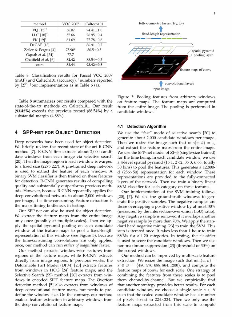
method VOC 2007 Caltech101

VQ [15]† 56.07 74.41±1.0LLC [18]† 57.66 76.95±0.4FK [19]† 61.69 77.78±0.6

DeCAF [13] - 86.91±0.7Zeiler & Fergus [4] 75.90‡ 86.5±0.5

Oquab et al. [34] 77.7 -Chatfield et al. [6] 82.42 88.54±0.3

ours 82.44 93.42±0.5

Table 8: Classification results for Pascal VOC 2007(mAP) and Caltech101 (accuracy). †numbers reportedby [27]. ‡our implementation as in Table 6 (a).

Table 8 summarizes our results compared with thestate-of-the-art methods on Caltech101. Our result(93.42%) exceeds the previous record (88.54%) by asubstantial margin (4.88%).

4 SPP-NET FOR OBJECT DETECTION

Deep networks have been used for object detection.We briefly review the recent state-of-the-art R-CNNmethod [7]. R-CNN first extracts about 2,000 candi-date windows from each image via selective search[20]. Then the image region in each window is warpedto a fixed size (227×227). A pre-trained deep networkis used to extract the feature of each window. Abinary SVM classifier is then trained on these featuresfor detection. R-CNN generates results of compellingquality and substantially outperforms previous meth-ods. However, because R-CNN repeatedly applies thedeep convolutional network to about 2,000 windowsper image, it is time-consuming. Feature extraction isthe major timing bottleneck in testing.

Our SPP-net can also be used for object detection.We extract the feature maps from the entire imageonly once (possibly at multiple scales). Then we ap-ply the spatial pyramid pooling on each candidatewindow of the feature maps to pool a fixed-lengthrepresentation of this window (see Figure 5). Becausethe time-consuming convolutions are only appliedonce, our method can run orders of magnitude faster.

Our method extracts window-wise features fromregions of the feature maps, while R-CNN extractsdirectly from image regions. In previous works, theDeformable Part Model (DPM) [23] extracts featuresfrom windows in HOG [24] feature maps, and theSelective Search (SS) method [20] extracts from win-dows in encoded SIFT feature maps. The Overfeatdetection method [5] also extracts from windows ofdeep convolutional feature maps, but needs to pre-define the window size. On the contrary, our methodenables feature extraction in arbitrary windows fromthe deep convolutional feature maps.

spatial pyramid

pooling layer

feature maps of conv5

convolutional layers

fixed-length representation

input image

window

…...

fully-connected layers (fc6, fc7)

Figure 5: Pooling features from arbitrary windowson feature maps. The feature maps are computedfrom the entire image. The pooling is performed incandidate windows.

4.1 Detection Algorithm

We use the “fast” mode of selective search [20] togenerate about 2,000 candidate windows per image.Then we resize the image such that min(w, h) = s,and extract the feature maps from the entire image.We use the SPP-net model of ZF-5 (single-size trained)for the time being. In each candidate window, we usea 4-level spatial pyramid (1×1, 2×2, 3×3, 6×6, totally50 bins) to pool the features. This generates a 12,800-d (256×50) representation for each window. Theserepresentations are provided to the fully-connectedlayers of the network. Then we train a binary linearSVM classifier for each category on these features.

Our implementation of the SVM training follows[20], [7]. We use the ground-truth windows to gen-erate the positive samples. The negative samples arethose overlapping a positive window by at most 30%(measured by the intersection-over-union (IoU) ratio).Any negative sample is removed if it overlaps anothernegative sample by more than 70%. We apply the stan-dard hard negative mining [23] to train the SVM. Thisstep is iterated once. It takes less than 1 hour to trainSVMs for all 20 categories. In testing, the classifieris used to score the candidate windows. Then we usenon-maximum suppression [23] (threshold of 30%) onthe scored windows.

Our method can be improved by multi-scale featureextraction. We resize the image such that min(w, h) =s ∈ S = {480, 576, 688, 864, 1200}, and compute thefeature maps of conv5 for each scale. One strategy ofcombining the features from these scales is to poolthem channel-by-channel. But we empirically findthat another strategy provides better results. For eachcandidate window, we choose a single scale s ∈ Ssuch that the scaled candidate window has a numberof pixels closest to 224×224. Then we only use thefeature maps extracted from this scale to compute

10

the feature of this window. If the pre-defined scalesare dense enough and the window is approximatelysquare, our method is roughly equivalent to resizingthe window to 224×224 and then extracting featuresfrom it. Nevertheless, our method only requires com-puting the feature maps once (at each scale) from theentire image, regardless of the number of candidatewindows.

We also fine-tune our pre-trained network, follow-ing [7]. Since our features are pooled from the conv5

feature maps from windows of any sizes, for sim-plicity we only fine-tune the fully-connected layers.In this case, the data layer accepts the fixed-lengthpooled features after conv5, and the fc6,7 layers anda new 21-way (one extra negative category) fc8 layerfollow. The fc8 weights are initialized with a Gaussiandistribution of σ=0.01. We fix all the learning rates to1e-4 and then adjust to 1e-5 for all three layers. Duringfine-tuning, the positive samples are those overlap-ping with a ground-truth window by [0.5, 1], andthe negative samples by [0.1, 0.5). In each mini-batch,25% of the samples are positive. We train 250k mini-batches using the learning rate 1e-4, and then 50kmini-batches using 1e-5. Because we only fine-tunethe fc layers, the training is very fast and takes about2 hours on the GPU (excluding pre-caching featuremaps which takes about 1 hour). Also following [7],we use bounding box regression to post-process theprediction windows. The features used for regressionare the pooled features from conv5 (as a counterpartof the pool5 features used in [7]). The windows usedfor the regression training are those overlapping witha ground-truth window by at least 50%.

4.2 Detection Results

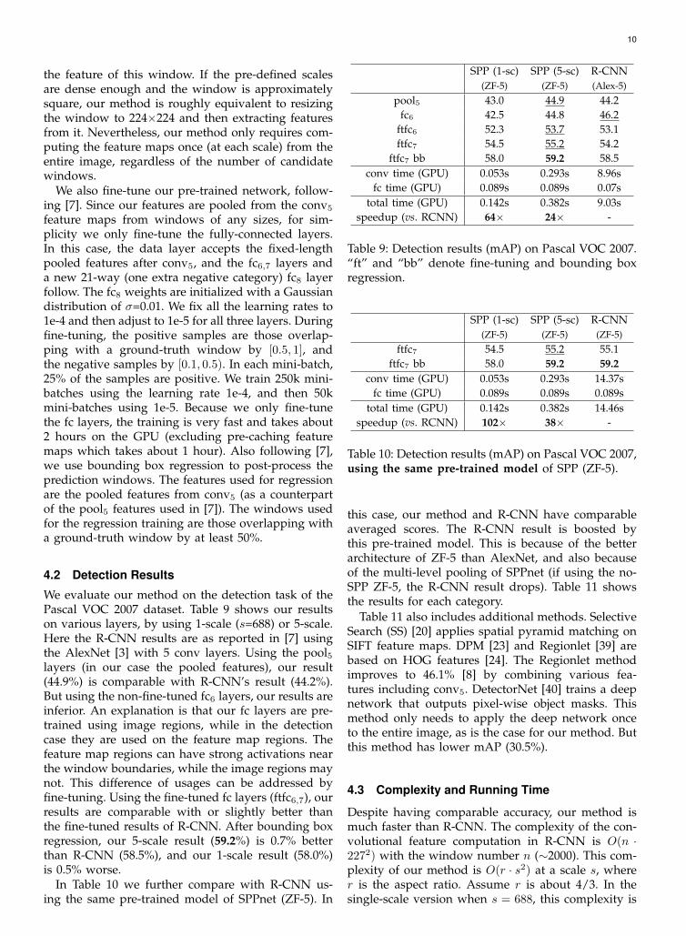
We evaluate our method on the detection task of thePascal VOC 2007 dataset. Table 9 shows our resultson various layers, by using 1-scale (s=688) or 5-scale.Here the R-CNN results are as reported in [7] usingthe AlexNet [3] with 5 conv layers. Using the pool5layers (in our case the pooled features), our result(44.9%) is comparable with R-CNN’s result (44.2%).But using the non-fine-tuned fc6 layers, our results areinferior. An explanation is that our fc layers are pre-trained using image regions, while in the detectioncase they are used on the feature map regions. Thefeature map regions can have strong activations nearthe window boundaries, while the image regions maynot. This difference of usages can be addressed byfine-tuning. Using the fine-tuned fc layers (ftfc6,7), ourresults are comparable with or slightly better thanthe fine-tuned results of R-CNN. After bounding boxregression, our 5-scale result (59.2%) is 0.7% betterthan R-CNN (58.5%), and our 1-scale result (58.0%)is 0.5% worse.

In Table 10 we further compare with R-CNN us-ing the same pre-trained model of SPPnet (ZF-5). In

SPP (1-sc) SPP (5-sc) R-CNN(ZF-5) (ZF-5) (Alex-5)

pool5 43.0 44.9 44.2fc6 42.5 44.8 46.2

ftfc6 52.3 53.7 53.1ftfc7 54.5 55.2 54.2

ftfc7 bb 58.0 59.2 58.5conv time (GPU) 0.053s 0.293s 8.96s

fc time (GPU) 0.089s 0.089s 0.07stotal time (GPU) 0.142s 0.382s 9.03s

speedup (vs. RCNN) 64× 24× -

Table 9: Detection results (mAP) on Pascal VOC 2007.“ft” and “bb” denote fine-tuning and bounding boxregression.

SPP (1-sc) SPP (5-sc) R-CNN(ZF-5) (ZF-5) (ZF-5)

ftfc7 54.5 55.2 55.1ftfc7 bb 58.0 59.2 59.2

conv time (GPU) 0.053s 0.293s 14.37sfc time (GPU) 0.089s 0.089s 0.089s

total time (GPU) 0.142s 0.382s 14.46sspeedup (vs. RCNN) 102× 38× -

Table 10: Detection results (mAP) on Pascal VOC 2007,using the same pre-trained model of SPP (ZF-5).

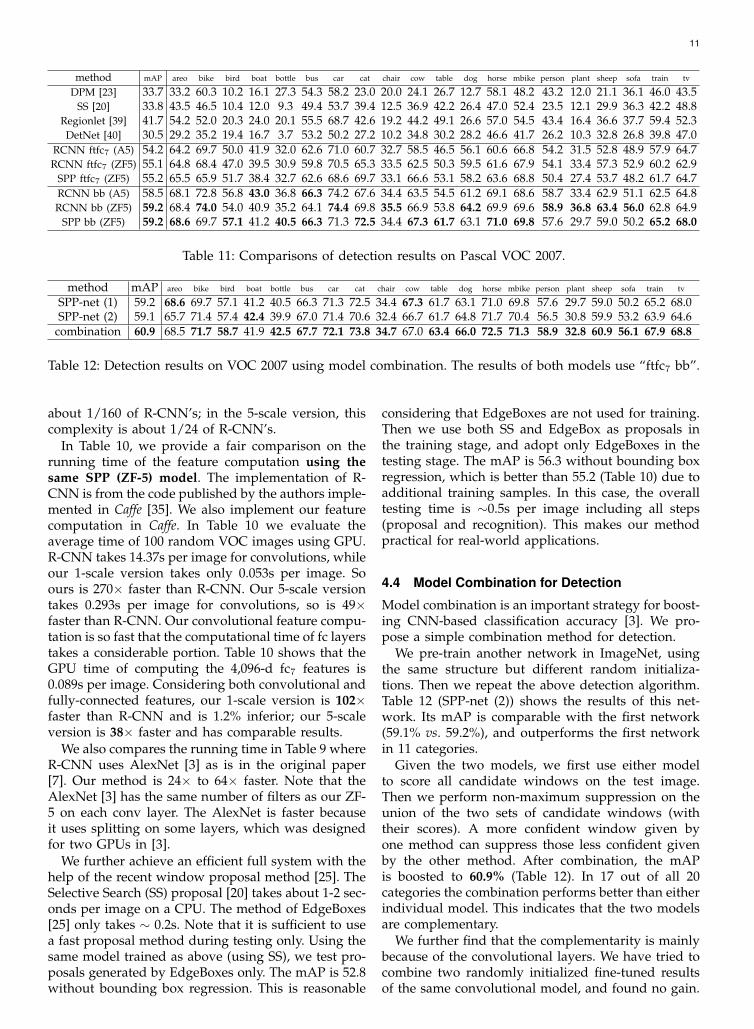
this case, our method and R-CNN have comparableaveraged scores. The R-CNN result is boosted bythis pre-trained model. This is because of the betterarchitecture of ZF-5 than AlexNet, and also becauseof the multi-level pooling of SPPnet (if using the no-SPP ZF-5, the R-CNN result drops). Table 11 showsthe results for each category.

Table 11 also includes additional methods. SelectiveSearch (SS) [20] applies spatial pyramid matching onSIFT feature maps. DPM [23] and Regionlet [39] arebased on HOG features [24]. The Regionlet methodimproves to 46.1% [8] by combining various fea-tures including conv5. DetectorNet [40] trains a deepnetwork that outputs pixel-wise object masks. Thismethod only needs to apply the deep network onceto the entire image, as is the case for our method. Butthis method has lower mAP (30.5%).

4.3 Complexity and Running Time

Despite having comparable accuracy, our method ismuch faster than R-CNN. The complexity of the con-volutional feature computation in R-CNN is O(n ·2272) with the window number n (∼2000). This com-plexity of our method is O(r · s2) at a scale s, wherer is the aspect ratio. Assume r is about 4/3. In thesingle-scale version when s = 688, this complexity is

11

method mAP areo bike bird boat bottle bus car cat chair cow table dog horse mbike person plant sheep sofa train tv

DPM [23] 33.7 33.2 60.3 10.2 16.1 27.3 54.3 58.2 23.0 20.0 24.1 26.7 12.7 58.1 48.2 43.2 12.0 21.1 36.1 46.0 43.5SS [20] 33.8 43.5 46.5 10.4 12.0 9.3 49.4 53.7 39.4 12.5 36.9 42.2 26.4 47.0 52.4 23.5 12.1 29.9 36.3 42.2 48.8

Regionlet [39] 41.7 54.2 52.0 20.3 24.0 20.1 55.5 68.7 42.6 19.2 44.2 49.1 26.6 57.0 54.5 43.4 16.4 36.6 37.7 59.4 52.3DetNet [40] 30.5 29.2 35.2 19.4 16.7 3.7 53.2 50.2 27.2 10.2 34.8 30.2 28.2 46.6 41.7 26.2 10.3 32.8 26.8 39.8 47.0

RCNN ftfc7 (A5) 54.2 64.2 69.7 50.0 41.9 32.0 62.6 71.0 60.7 32.7 58.5 46.5 56.1 60.6 66.8 54.2 31.5 52.8 48.9 57.9 64.7RCNN ftfc7 (ZF5) 55.1 64.8 68.4 47.0 39.5 30.9 59.8 70.5 65.3 33.5 62.5 50.3 59.5 61.6 67.9 54.1 33.4 57.3 52.9 60.2 62.9

SPP ftfc7 (ZF5) 55.2 65.5 65.9 51.7 38.4 32.7 62.6 68.6 69.7 33.1 66.6 53.1 58.2 63.6 68.8 50.4 27.4 53.7 48.2 61.7 64.7RCNN bb (A5) 58.5 68.1 72.8 56.8 43.0 36.8 66.3 74.2 67.6 34.4 63.5 54.5 61.2 69.1 68.6 58.7 33.4 62.9 51.1 62.5 64.8RCNN bb (ZF5) 59.2 68.4 74.0 54.0 40.9 35.2 64.1 74.4 69.8 35.5 66.9 53.8 64.2 69.9 69.6 58.9 36.8 63.4 56.0 62.8 64.9

SPP bb (ZF5) 59.2 68.6 69.7 57.1 41.2 40.5 66.3 71.3 72.5 34.4 67.3 61.7 63.1 71.0 69.8 57.6 29.7 59.0 50.2 65.2 68.0

Table 11: Comparisons of detection results on Pascal VOC 2007.

method mAP areo bike bird boat bottle bus car cat chair cow table dog horse mbike person plant sheep sofa train tv

SPP-net (1) 59.2 68.6 69.7 57.1 41.2 40.5 66.3 71.3 72.5 34.4 67.3 61.7 63.1 71.0 69.8 57.6 29.7 59.0 50.2 65.2 68.0SPP-net (2) 59.1 65.7 71.4 57.4 42.4 39.9 67.0 71.4 70.6 32.4 66.7 61.7 64.8 71.7 70.4 56.5 30.8 59.9 53.2 63.9 64.6

combination 60.9 68.5 71.7 58.7 41.9 42.5 67.7 72.1 73.8 34.7 67.0 63.4 66.0 72.5 71.3 58.9 32.8 60.9 56.1 67.9 68.8

Table 12: Detection results on VOC 2007 using model combination. The results of both models use “ftfc7 bb”.

about 1/160 of R-CNN’s; in the 5-scale version, thiscomplexity is about 1/24 of R-CNN’s.

In Table 10, we provide a fair comparison on therunning time of the feature computation using thesame SPP (ZF-5) model. The implementation of R-CNN is from the code published by the authors imple-mented in Caffe [35]. We also implement our featurecomputation in Caffe. In Table 10 we evaluate theaverage time of 100 random VOC images using GPU.R-CNN takes 14.37s per image for convolutions, whileour 1-scale version takes only 0.053s per image. Soours is 270× faster than R-CNN. Our 5-scale versiontakes 0.293s per image for convolutions, so is 49×faster than R-CNN. Our convolutional feature compu-tation is so fast that the computational time of fc layerstakes a considerable portion. Table 10 shows that theGPU time of computing the 4,096-d fc7 features is0.089s per image. Considering both convolutional andfully-connected features, our 1-scale version is 102×faster than R-CNN and is 1.2% inferior; our 5-scaleversion is 38× faster and has comparable results.

We also compares the running time in Table 9 whereR-CNN uses AlexNet [3] as is in the original paper[7]. Our method is 24× to 64× faster. Note that theAlexNet [3] has the same number of filters as our ZF-5 on each conv layer. The AlexNet is faster becauseit uses splitting on some layers, which was designedfor two GPUs in [3].

We further achieve an efficient full system with thehelp of the recent window proposal method [25]. TheSelective Search (SS) proposal [20] takes about 1-2 sec-onds per image on a CPU. The method of EdgeBoxes[25] only takes ∼ 0.2s. Note that it is sufficient to usea fast proposal method during testing only. Using thesame model trained as above (using SS), we test pro-posals generated by EdgeBoxes only. The mAP is 52.8without bounding box regression. This is reasonable

considering that EdgeBoxes are not used for training.Then we use both SS and EdgeBox as proposals inthe training stage, and adopt only EdgeBoxes in thetesting stage. The mAP is 56.3 without bounding boxregression, which is better than 55.2 (Table 10) due toadditional training samples. In this case, the overalltesting time is ∼0.5s per image including all steps(proposal and recognition). This makes our methodpractical for real-world applications.

4.4 Model Combination for Detection

Model combination is an important strategy for boost-ing CNN-based classification accuracy [3]. We pro-pose a simple combination method for detection.

We pre-train another network in ImageNet, usingthe same structure but different random initializa-tions. Then we repeat the above detection algorithm.Table 12 (SPP-net (2)) shows the results of this net-work. Its mAP is comparable with the first network(59.1% vs. 59.2%), and outperforms the first networkin 11 categories.

Given the two models, we first use either modelto score all candidate windows on the test image.Then we perform non-maximum suppression on theunion of the two sets of candidate windows (withtheir scores). A more confident window given byone method can suppress those less confident givenby the other method. After combination, the mAPis boosted to 60.9% (Table 12). In 17 out of all 20categories the combination performs better than eitherindividual model. This indicates that the two modelsare complementary.

We further find that the complementarity is mainlybecause of the convolutional layers. We have tried tocombine two randomly initialized fine-tuned resultsof the same convolutional model, and found no gain.

12

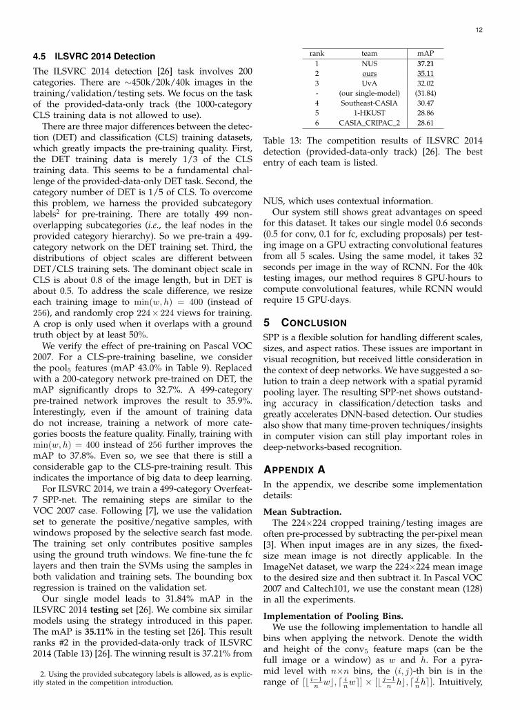
4.5 ILSVRC 2014 Detection

The ILSVRC 2014 detection [26] task involves 200categories. There are ∼450k/20k/40k images in thetraining/validation/testing sets. We focus on the taskof the provided-data-only track (the 1000-categoryCLS training data is not allowed to use).

There are three major differences between the detec-tion (DET) and classification (CLS) training datasets,which greatly impacts the pre-training quality. First,the DET training data is merely 1/3 of the CLStraining data. This seems to be a fundamental chal-lenge of the provided-data-only DET task. Second, thecategory number of DET is 1/5 of CLS. To overcomethis problem, we harness the provided subcategorylabels2 for pre-training. There are totally 499 non-overlapping subcategories (i.e., the leaf nodes in theprovided category hierarchy). So we pre-train a 499-category network on the DET training set. Third, thedistributions of object scales are different betweenDET/CLS training sets. The dominant object scale inCLS is about 0.8 of the image length, but in DET isabout 0.5. To address the scale difference, we resizeeach training image to min(w, h) = 400 (instead of256), and randomly crop 224×224 views for training.A crop is only used when it overlaps with a groundtruth object by at least 50%.

We verify the effect of pre-training on Pascal VOC2007. For a CLS-pre-training baseline, we considerthe pool5 features (mAP 43.0% in Table 9). Replacedwith a 200-category network pre-trained on DET, themAP significantly drops to 32.7%. A 499-categorypre-trained network improves the result to 35.9%.Interestingly, even if the amount of training datado not increase, training a network of more cate-gories boosts the feature quality. Finally, training withmin(w, h) = 400 instead of 256 further improves themAP to 37.8%. Even so, we see that there is still aconsiderable gap to the CLS-pre-training result. Thisindicates the importance of big data to deep learning.

For ILSVRC 2014, we train a 499-category Overfeat-7 SPP-net. The remaining steps are similar to theVOC 2007 case. Following [7], we use the validationset to generate the positive/negative samples, withwindows proposed by the selective search fast mode.The training set only contributes positive samplesusing the ground truth windows. We fine-tune the fclayers and then train the SVMs using the samples inboth validation and training sets. The bounding boxregression is trained on the validation set.

Our single model leads to 31.84% mAP in theILSVRC 2014 testing set [26]. We combine six similarmodels using the strategy introduced in this paper.The mAP is 35.11% in the testing set [26]. This resultranks #2 in the provided-data-only track of ILSVRC2014 (Table 13) [26]. The winning result is 37.21% from

2. Using the provided subcategory labels is allowed, as is explic-itly stated in the competition introduction.

rank team mAP1 NUS 37.212 ours 35.113 UvA 32.02- (our single-model) (31.84)4 Southeast-CASIA 30.475 1-HKUST 28.866 CASIA CRIPAC 2 28.61

Table 13: The competition results of ILSVRC 2014detection (provided-data-only track) [26]. The bestentry of each team is listed.

NUS, which uses contextual information.Our system still shows great advantages on speed

for this dataset. It takes our single model 0.6 seconds(0.5 for conv, 0.1 for fc, excluding proposals) per test-ing image on a GPU extracting convolutional featuresfrom all 5 scales. Using the same model, it takes 32seconds per image in the way of RCNN. For the 40ktesting images, our method requires 8 GPU·hours tocompute convolutional features, while RCNN wouldrequire 15 GPU·days.

5 CONCLUSION

SPP is a flexible solution for handling different scales,sizes, and aspect ratios. These issues are important invisual recognition, but received little consideration inthe context of deep networks. We have suggested a so-lution to train a deep network with a spatial pyramidpooling layer. The resulting SPP-net shows outstand-ing accuracy in classification/detection tasks andgreatly accelerates DNN-based detection. Our studiesalso show that many time-proven techniques/insightsin computer vision can still play important roles indeep-networks-based recognition.

APPENDIX AIn the appendix, we describe some implementationdetails:

Mean Subtraction.The 224×224 cropped training/testing images are

often pre-processed by subtracting the per-pixel mean[3]. When input images are in any sizes, the fixed-size mean image is not directly applicable. In theImageNet dataset, we warp the 224×224 mean imageto the desired size and then subtract it. In Pascal VOC2007 and Caltech101, we use the constant mean (128)in all the experiments.

Implementation of Pooling Bins.We use the following implementation to handle all

bins when applying the network. Denote the widthand height of the conv5 feature maps (can be thefull image or a window) as w and h. For a pyra-mid level with n×n bins, the (i, j)-th bin is in therange of [b i−1n wc, d inwe] × [b j−1n hc, d jnhe]. Intuitively,

13

bottle :0.24

person:1.20

sheep:1.52

chair:0.21

diningtable:0.78

person:1.16person:1.05

pottedplant:0 .21

chair:4.79

pottedplant:0.73

chai r:0 .33

din ingtable:0.34

chair:0.89

bus:0.56

car:3.24

car:3.45

person:1.52

train:0.31

train:1.62

pottedplant:0.33

pottedplant:0.78

sofa:0.55tvmonitor:1.77

aeroplane:0.45

aeroplane:1.40

aeroplane:1.01

aeroplane:0.94

aeroplane:0.93

aeroplane:0.91 aeroplane:0.79

aeroplane:0.57aeroplane:0.54

person:0.93

person:0.68

horse:1.73

person:1.91

boat:0.60

person:3.20

car:2.52

bus:2.01

car:0.93person:4.16

person:0.79

person:0.32

horse:1.68

horse:0.61

horse:1.29

person:1.23

chair:0.87

person:1.79

person:0.91

sofa:0.22

person:0.85sofa:0.58

cow:2.36

cow:1.88

cow:1.86

cow:1.82

cow:1.39cow:1.31

cat:0.52

person:1.02

person:0.40

bicycle:2.85

bicycle:2.71

bicycle:2.04

bicycle:0.67

person:3.35person:2.39

person:2.11

person:0.27

person:0.22

bus:1.42

person:3.29

person:1.18

bottle:1.15pottedplant:0.81

sheep:1.81

sheep:1.17

sheep:0.81

bird:0.24

pottedplant:0.35pottedplant:0.20

car:1.31person:1.60

person:0.62

dog:0.37

person:0 .38

dog:0.99

person:1.48

person:0.22

cow:0.80

person:3.29

person:2.69

person:2.42person:1.05

person:0.92person:0.76

bird:1.39bird:0.84

bottle:1.20diningtable:0.96

person:1.53

person:1.52

person:0.73

car:0.12

car:0.11

car:0.04

car:0.03

car:3.98

car:1.95

car:1.39

car:0.50

bird:1.47

sofa:0.41 person:2.15

person:0.86

tvmonitor:2.24

motorbike:1.11motorbike:0.74

person:1.36

person:1.10

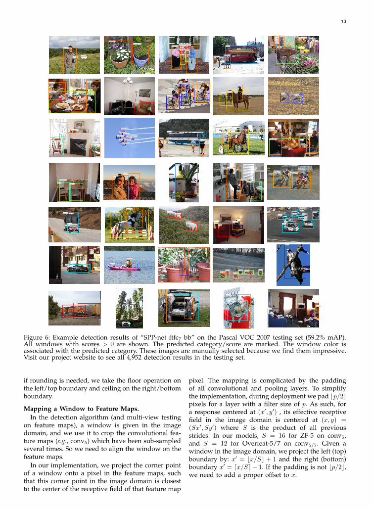
Figure 6: Example detection results of “SPP-net ftfc7 bb” on the Pascal VOC 2007 testing set (59.2% mAP).All windows with scores > 0 are shown. The predicted category/score are marked. The window color isassociated with the predicted category. These images are manually selected because we find them impressive.Visit our project website to see all 4,952 detection results in the testing set.

if rounding is needed, we take the floor operation onthe left/top boundary and ceiling on the right/bottomboundary.

Mapping a Window to Feature Maps.In the detection algorithm (and multi-view testing

on feature maps), a window is given in the imagedomain, and we use it to crop the convolutional fea-ture maps (e.g., conv5) which have been sub-sampledseveral times. So we need to align the window on thefeature maps.

In our implementation, we project the corner pointof a window onto a pixel in the feature maps, suchthat this corner point in the image domain is closestto the center of the receptive field of that feature map

pixel. The mapping is complicated by the paddingof all convolutional and pooling layers. To simplifythe implementation, during deployment we pad bp/2cpixels for a layer with a filter size of p. As such, fora response centered at (x′, y′) , its effective receptivefield in the image domain is centered at (x, y) =(Sx′, Sy′) where S is the product of all previousstrides. In our models, S = 16 for ZF-5 on conv5,and S = 12 for Overfeat-5/7 on conv5/7. Given awindow in the image domain, we project the left (top)boundary by: x′ = bx/Sc + 1 and the right (bottom)boundary x′ = dx/Se − 1. If the padding is not bp/2c,we need to add a proper offset to x.

14

REFERENCES[1] Y. LeCun, B. Boser, J. S. Denker, D. Henderson, R. E. Howard,

W. Hubbard, and L. D. Jackel, “Backpropagation applied tohandwritten zip code recognition,” Neural computation, 1989.

[2] J. Deng, W. Dong, R. Socher, L.-J. Li, K. Li, and L. Fei-Fei, “Imagenet: A large-scale hierarchical image database,” inCVPR, 2009.

[3] A. Krizhevsky, I. Sutskever, and G. Hinton, “Imagenet classi-fication with deep convolutional neural networks,” in NIPS,2012.

[4] M. D. Zeiler and R. Fergus, “Visualizing and understandingconvolutional neural networks,” arXiv:1311.2901, 2013.

[5] P. Sermanet, D. Eigen, X. Zhang, M. Mathieu, R. Fergus,and Y. LeCun, “Overfeat: Integrated recognition, localizationand detection using convolutional networks,” arXiv:1312.6229,2013.

[6] A. V. K. Chatfield, K. Simonyan and A. Zisserman, “Return ofthe devil in the details: Delving deep into convolutional nets,”in ArXiv:1405.3531, 2014.

[7] R. Girshick, J. Donahue, T. Darrell, and J. Malik, “Rich featurehierarchies for accurate object detection and semantic segmen-tation,” in CVPR, 2014.

[8] W. Y. Zou, X. Wang, M. Sun, and Y. Lin, “Generic ob-ject detection with dense neural patterns and regionlets,” inArXiv:1404.4316, 2014.

[9] A. S. Razavian, H. Azizpour, J. Sullivan, and S. Carlsson, “Cnnfeatures off-the-shelf: An astounding baseline for recogniton,”in CVPR 2014, DeepVision Workshop, 2014.

[10] Y. Taigman, M. Yang, M. Ranzato, and L. Wolf, “Deepface:Closing the gap to human-level performance in face verifica-tion,” in CVPR, 2014.

[11] N. Zhang, M. Paluri, M. Ranzato, T. Darrell, and L. Bourdevr,“Panda: Pose aligned networks for deep attribute modeling,”in CVPR, 2014.

[12] Y. Gong, L. Wang, R. Guo, and S. Lazebnik, “Multi-scaleorderless pooling of deep convolutional activation features,”in ArXiv:1403.1840, 2014.

[13] J. Donahue, Y. Jia, O. Vinyals, J. Hoffman, N. Zhang, E. Tzeng,and T. Darrell, “Decaf: A deep convolutional activation featurefor generic visual recognition,” arXiv:1310.1531, 2013.

[14] K. Grauman and T. Darrell, “The pyramid match kernel:Discriminative classification with sets of image features,” inICCV, 2005.

[15] S. Lazebnik, C. Schmid, and J. Ponce, “Beyond bags of fea-tures: Spatial pyramid matching for recognizing natural scenecategories,” in CVPR, 2006.

[16] J. Sivic and A. Zisserman, “Video google: a text retrievalapproach to object matching in videos,” in ICCV, 2003.

[17] J. Yang, K. Yu, Y. Gong, and T. Huang, “Linear spatial pyramidmatching using sparse coding for image classification,” inCVPR, 2009.

[18] J. Wang, J. Yang, K. Yu, F. Lv, T. Huang, and Y. Gong, “Locality-constrained linear coding for image classification,” in CVPR,2010.

[19] F. Perronnin, J. Sanchez, and T. Mensink, “Improving the fisherkernel for large-scale image classification,” in ECCV, 2010.

[20] K. E. van de Sande, J. R. Uijlings, T. Gevers, and A. W. Smeul-ders, “Segmentation as selective search for object recognition,”in ICCV, 2011.

[21] L. Fei-Fei, R. Fergus, and P. Perona, “Learning generativevisual models from few training examples: An incrementalbayesian approach tested on 101 object categories,” CVIU,2007.

[22] M. Everingham, L. Van Gool, C. K. I. Williams, J. Winn, andA. Zisserman, “The PASCAL Visual Object Classes Challenge2007 (VOC2007) Results,” 2007.

[23] P. F. Felzenszwalb, R. B. Girshick, D. McAllester, and D. Ra-manan, “Object detection with discriminatively trained part-based models,” PAMI, 2010.

[24] N. Dalal and B. Triggs, “Histograms of oriented gradients forhuman detection,” in CVPR, 2005.

[25] C. L. Zitnick and P. Dollar, “Edge boxes: Locating objectproposals from edges,” in ECCV, 2014.

[26] O. Russakovsky, J. Deng, H. Su, J. Krause, S. Satheesh,S. Ma, Z. Huang, A. Karpathy, A. Khosla, M. Bernsteinet al., “Imagenet large scale visual recognition challenge,”arXiv:1409.0575, 2014.

[27] K. Chatfield, V. Lempitsky, A. Vedaldi, and A. Zisserman, “Thedevil is in the details: an evaluation of recent feature encodingmethods,” in BMVC, 2011.

[28] A. Coates and A. Ng, “The importance of encoding versustraining with sparse coding and vector quantization,” in ICML,2011.

[29] D. G. Lowe, “Distinctive image features from scale-invariantkeypoints,” IJCV, 2004.

[30] J. C. van Gemert, J.-M. Geusebroek, C. J. Veenman, and A. W.Smeulders, “Kernel codebooks for scene categorization,” inECCV, 2008.

[31] M. Lin, Q. Chen, and S. Yan, “Network in network,”arXiv:1312.4400, 2013.

[32] C. Szegedy, W. Liu, Y. Jia, P. Sermanet, S. Reed, D. Anguelov,D. Erhan, V. Vanhoucke, and A. Rabinovich, “Going deeperwith convolutions,” arXiv:1409.4842, 2014.

[33] K. Simonyan and A. Zisserman, “Very deep convolutionalnetworks for large-scale image recognition,” arXiv:1409.1556,2014.

[34] M. Oquab, L. Bottou, I. Laptev, J. Sivic et al., “Learning andtransferring mid-level image representations using convolu-tional neural networks,” in CVPR, 2014.

[35] Y. Jia, “Caffe: An open source convolutional architecturefor fast feature embedding,” http://caffe.berkeleyvision.org/,2013.

[36] A. G. Howard, “Some improvements on deep convolutionalneural network based image classification,” ArXiv:1312.5402,2013.

[37] H. Jegou, F. Perronnin, M. Douze, J. Sanchez, P. Perez, andC. Schmid, “Aggregating local image descriptors into compactcodes,” TPAMI, vol. 34, no. 9, pp. 1704–1716, 2012.

[38] C.-C. Chang and C.-J. Lin, “Libsvm: a library for supportvector machines,” ACM Transactions on Intelligent Systems andTechnology (TIST), 2011.

[39] X. Wang, M. Yang, S. Zhu, and Y. Lin, “Regionlets for genericobject detection,” in ICCV, 2013.

[40] C. Szegedy, A. Toshev, and D. Erhan, “Deep neural networksfor object detection,” in NIPS, 2013.

CHANGELOG

arXiv v1. Initial technical report for ECCV 2014 paper.

arXiv v2. Submitted version for TPAMI. Includes extraexperiments of SPP on various architectures. Includesdetails for ILSVRC 2014.

arXiv v3. Accepted version for TPAMI. Includes com-parisons with R-CNN using the same architecture.Includes detection experiments using EdgeBoxes.

arXiv v4. Revised “Mapping a Window to FeatureMaps” in Appendix for easier implementation.