Spatial patterns of growth and poverty changes in Peru ... · Spatial patterns of growth and...

Spatial patterns of growth and poverty changes in Peru

(1993 – 2005)

Javier Escobal y Carmen Ponce

Documento de Trabajo N° 78 Programa Dinámicas Territoriales Rurales

Rimisp – Centro Latinoamericano para el Desarrollo Rural

P á g i n a | 2

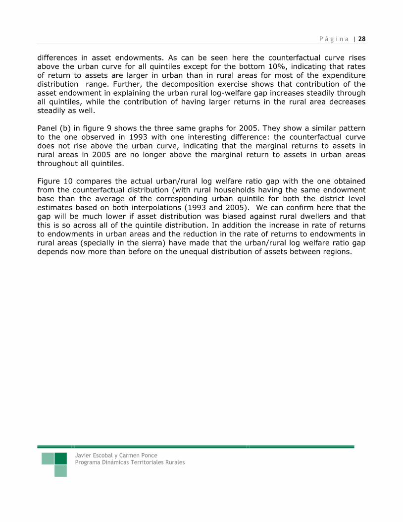
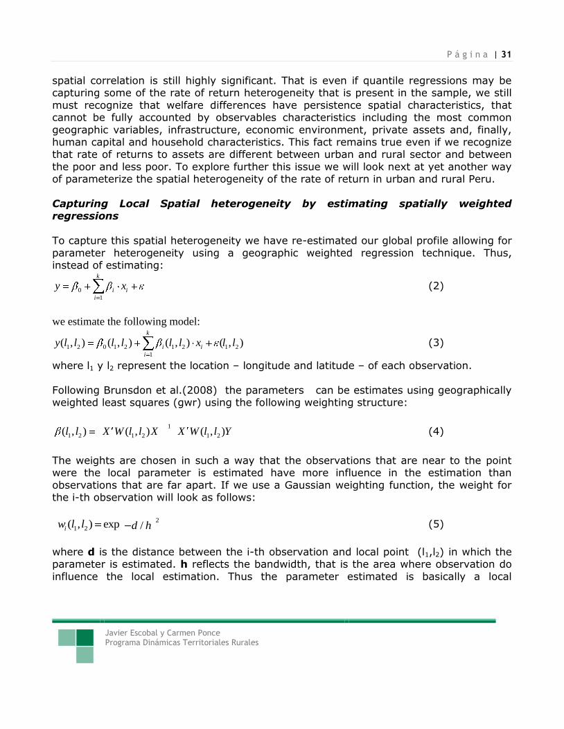
Javier Escobal y Carmen Ponce Programa Dinámicas Territoriales Rurales

Este documento es el resultado del

Programa Dinámicas Territoriales Rurales,

que Rimisp lleva a cabo en varios países

de América Latina en colaboración con

numerosos socios. El programa cuenta con

el auspicio del Centro Internacional de

Investigaciones para el Desarrollo (IDRC,

Canadá). Se autoriza la reproducción

parcial o total y la difusión del documento

sin fines de lucro y sujeta a que se cite la

fuente.

This document is the result of the Rural

Territorial Dynamics Program,

implemented by Rimisp in several Latin

American countries in collaboration with

numerous partners. The program has been

supported by the International

Development Research Center (IDRC,

Canada). We authorize the non-for-profit

partial or full reproduction and

dissemination of this document, subject

to the source being properly

acknowledged.

Cita / Citation:

Escobal, J. y Ponce, C. 2011. “Spatial Patterns of Growth and Poverty Changes in Peru (1993 – 2005)”. Documento de Trabajo N° 78. Programa Dinámicas Territoriales Rurales. Rimisp, Santiago, Chile.

© Rimisp-Centro Latinoamericano para el

Desarrollo Rural

Programa Dinámicas Territoriales Rurales

Casilla 228-22

Santiago, Chile

Tel + (56-2) 236 45 57

[email protected]

www.rimisp.org/dtr

http://www.rimisp.org/dtr

P á g i n a | 1


Índice

1. Introduction ...................................................................................................... 2

2. Small area Estimates of Poverty in Peru ................................................................ 3

2.1 Mean Characteristics of districts showing significant poverty changes ................ 10

2.2 Poverty profiles .......................................................................................... 14

2.3 Spatial Correlation ...................................................................................... 19

2.4 Is Geography Destiny?: looking at spatial heterogeneity in Peruvian welfare

dynamics. ........................................................................................................... 22

2.5 Spatial heterogeneity: looking beyond the Global Model .................................. 27

3. Final Remarks ............................................................................................... 40

4. References .................................................................................................... 42

P á g i n a | 2


1. Introduction

The period that spanned between the last two population censuses (1993 and 2005) in Peru can be characterized as a period of economic growth. In this period the Peruvian

economy grew at an annual average rate of 5%. Nevertheless, this positive trend was not homogeneous within the country. Urban areas experienced a higher pace of growth than rural areas and, within the latter, there is evidence of increasing gaps in favor of the

Coastal Region as compared to the Highlands and Amazon regions (Vakis et al. 2008).

Given the important methodological changes in the calculation of poverty statistics (to the extent to seriously affect their comparability across years (Herrera, 2002)), it is difficult to assess how this uneven growth affected household wellbeing throughout the

country. Further, poverty estimates are available at high levels of aggregation only and cannot be used to study spatial patterns at local levels. The purpose of this paper is to

document the uneven growth and poverty dynamics occurred in Peru in the period 1993-2005 and evaluate up to what point spatial characteristics affect wellbeing levels and changes of Peruvian households.

In order to estimate poverty dynamics at local levels (lower aggregation levels than

those normally obtained in nationally representative households surveys), two poverty mapping estimations are performed. The first poverty mapping exercise combines the

1993 population census, with the 1994 LSMS Survey and a number of district and province1 level characteristics coming from the 1994 Agriculture Census and the district-level municipality censuses. The second poverty mapping exercise combines the 2005

population census, with the 2006 Household Survey (ENAHO) and the previously mentioned databases for district and province level characteristics as well as a provincial

representative survey (ENCO). The following section constitutes the core of the paper and it starts with the discussion of the main findings of poverty dynamics estimates. The first two subsections explore the potential role of key public and private assets on

experiencing positive poverty trajectories. The last three subsections in turn, discuss identification problems associated with the spatial dimension of poverty dynamics

estimation.

1 The lower level of public administrative hierarchy is the district. Districts are grouped in provinces, which in turn are grouped in departments (also named regions).

P á g i n a | 3


2. Small area Estimates of Poverty in Peru

To estimate Poverty rates at low level of spatial aggregation we have combined several

data sources to construct per-capita expenditure estimates for each household in both the Peruvian 1993 and 2005 Population Censuses. The methodology used, follows closely Elbers, et al (2003). Table 1 presents a comparison of the estimated poverty rates and

their standard errors for each of the two census years and the household surveys. This comparison is done at the level of aggregation at which each of the two household

surveys can generate statistically representative results. It is important to note that the comparison needs to be done with caution. First, in both cases the interpolation is done for the previous year than the ones where the household surveys were collected (1993

instead of 1994 and 2005 instead of 2006). Second, since the sampling frame is not incorporated fully in the interpolation exercise the standard errors may be somewhat

underestimated. Further the fact that we do not account for the spatial correlation in the disturbances may be underestimating further the estimated standard errors2.

Table 1 Comparison of Regional Poverty Rates and Census Interpolations

FGT(0) est. dev. FGT(0) est. dev. FGT(0) est. dev. FGT(0) est. dev.

Urban Costa 43.9% 4.00% 48.2% 0.08% 30.2% 1.47% 34.1% 0.74%

Rural Costa 60.9% 5.61% 51.9% 0.10% 47.4% 2.80% 49.2% 0.87%

Urban Sierra 46.0% 4.10% 46.0% 0.09% 40.2% 1.71% 49.8% 1.77%

Rural Sierra 67.7% 2.64% 62.5% 0.05% 76.7% 1.12% 72.2% 0.70%

Urban Selva 39.6% 4.06% 45.3% 0.13% 50.6% 2.89% 52.8% 1.49%

Rural Selva 70.6% 3.40% 77.8% 0.17% 62.9% 1.72% 62.9% 0.69%

Metropolitan Lima 32.2% 2.39% 36.2% 0.05% 24.2% 1.37% 28.7% 0.88%

FGT(0) est. dev. FGT(0) est. dev. FGT(0) est. dev. FGT(0) est. dev.

Costa 47.8% 3.35% 49.6% 0.06% 34.1% 1.30% 37.1% 0.74%

Sierra 59.8% 2.28% 58.5% 0.04% 63.7% 1.00% 63.1% 0.82%

Selva 56.7% 2.63% 66.8% 0.09% 57.3% 1.54% 57.9% 0.85%

Metropolitan Lima 32.2% 2.39% 36.2% 0.05% 24.2% 1.37% 28.7% 0.88%

Peru 48.9% 1.27% 51.3% 0.07% 44.8% 0.69% 46.0% 0.96%

Census 1993

Interpolation ENNIV 1994 ENAHO 2006

Census 2005

Interpolation

Source: Own estimates base don Census interpolation and ENNIV 1994 and ENAHO 2005 surveys

In general our results do match with the estimated poverty rates in both years. In all

cases the estimated census interpolation falls within the 99% confidence interval of the household survey estimates. Still, if we test the differences using the standard deviation

2 Lanjouw et al (2007) uses pseudo samples obtained from Mexican data to contend that confidence intervals obtained from this small area methodology do correspond to what should be expected.

P á g i n a | 4


estimated in both household and census and we contend that these are independent samples the test will indicate that we cannot reject that estimates are equal in the 1993

for all regions and in most of the regions for 2005. Is interesting to note that the for 2005 the most important deviations occur in Lima, in urban Costa and in urban Sierra,

which are precisely the areas where poverty has been reduced the most between 2004 and 2006. In those three cases poverty rates in the census interpolation are slightly larger than the ENAHO 2006 estimates, which we believe is reasonable. In the case of

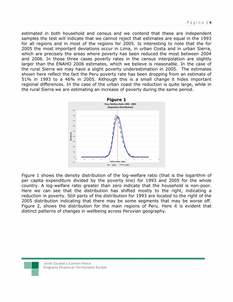
the rural Sierra we may have a slight poverty underestimation in 2005. The estimates shown here reflect the fact the Peru poverty rate has been dropping from an estimate of

51% in 1993 to a 46% in 2005. Although this is a small change it hides important regional differences. In the case of the urban coast the reduction is quite large, while in the rural Sierra we are estimating an increase of poverty during the same period.

Figure 1

Peru: Welfare Ratio 1993 - 2005

(Population Distrtibution)

-0.1

0

0.1

0.2

0.3

0.4

0.5

0.6

0.7

0.8

0.9

-5 -4 -3 -2 -1 0 1 2 3 4 5

Welfare Ratio (logs)

de

nsi

ty (

%)

1993 2005 Figure 1 shows the density distribution of the log-welfare ratio (that is the logarithm of per capita expenditure divided by the poverty line) for 1993 and 2005 for the whole

country. A log-welfare ratio greater than zero indicate that the household is non-poor. Here we can see that the distribution has shifted mostly to the right, indicating a

reduction in poverty. Still parts of the distribution for 1993 are located to the right of the 2005 distribution indicating that there may be some segments that may be worse off.

Figure 2, shows the distribution for the main regions of Peru. Here it is evident that distinct patterns of changes in wellbeing across Peruvian geography.

P á g i n a | 5


Figure 2 Log-Welfare Ratio Distribution by Geographic Region

(a) (b) 0

.2.4

.6.8

1

den

sity (

%)

-4 -2 0 2 4Welfare Ratio (logs)

1993 2005

(Population Distribution)

Costa Region: Welfare Ratio 1993 - 2005

0.2

.4.6

.81

den

sity (

%)


1993 2005


Sierra Region: Welfare Ratio 1993 - 2005

(c) (d)

0.5

11

.5

den

sity (

%)


1993 2005


Selva Region: Welfare Ratio 1993 - 2005

0.2

.4.6

.81

den

sity (

%)

-2 -1 0 1 2 3Welfare Ratio (logs)

1993 2005


Metropolitan Lima: Welfare Ratio 1993 - 2005

As we have mention, the use of household data plus census data, allow us to obtain

poverty estimates at greater disaggregation levels than the ones survey estimates can allow. In order to aid on the interpretation of the spatial patterns of poverty changes in

Peru, Figure 3 maps an estimation of growth at the district level occurred between 1993 and 2005, using our estimated welfare measure of per-capita expenditure. We have colored the map in growth ranges and considering ±1% per year as very little or no

growth, even if most of these districts may have been considered as having statistically significant changes if we have done a formal test3.

Figure 3 shows that although growth has been widespread across Peru during the 1993-

2005 period, areas with low or null growth tend to be spatially concentrated along the

3 We have preferred not do so on several grounds. First we recognize that although expenditure groups are the same in both surveys the detail of the questionnaire is much larger in the ENAHO 2005 which may generate some upward bias. Second, formal statistical testing between both interpolation need further elaboration (given that the estimation do share a number of right had side variables).

P á g i n a | 6


highlands of Peru. To make this even more evident, Figure 4 shows the altitude of all districts in Peru. Contrasting Figure 3 and Figure 4 shows clearly that those districts that

are located in high altitude areas are more likely to have shown low or null growth.

Figure 3

Per Capita Expenditure Growth 1993-2005

(Annual growth rates)

P á g i n a | 7


Figure 4

District Altitude

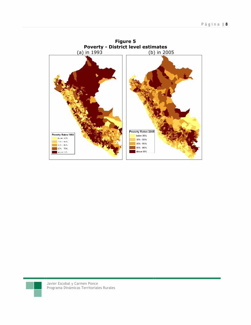
Given this patter of growth it is interesting to see how poverty has change between these

two census years. Figure 5 shows the poverty rates of all districts in Peru for 1993 and 2005 while Figure 6 shows the changes in these poverty rates at the district level.

P á g i n a | 8


Figure 5

Poverty - District level estimates (a) in 1993 (b) in 2005

P á g i n a | 9


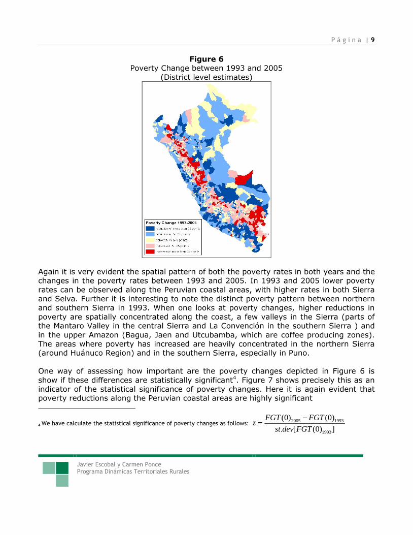
Figure 6 Poverty Change between 1993 and 2005

(District level estimates)

Again it is very evident the spatial pattern of both the poverty rates in both years and the changes in the poverty rates between 1993 and 2005. In 1993 and 2005 lower poverty

rates can be observed along the Peruvian coastal areas, with higher rates in both Sierra and Selva. Further it is interesting to note the distinct poverty pattern between northern and southern Sierra in 1993. When one looks at poverty changes, higher reductions in

poverty are spatially concentrated along the coast, a few valleys in the Sierra (parts of the Mantaro Valley in the central Sierra and La Convención in the southern Sierra ) and

in the upper Amazon (Bagua, Jaen and Utcubamba, which are coffee producing zones). The areas where poverty has increased are heavily concentrated in the northern Sierra (around Huánuco Region) and in the southern Sierra, especially in Puno.

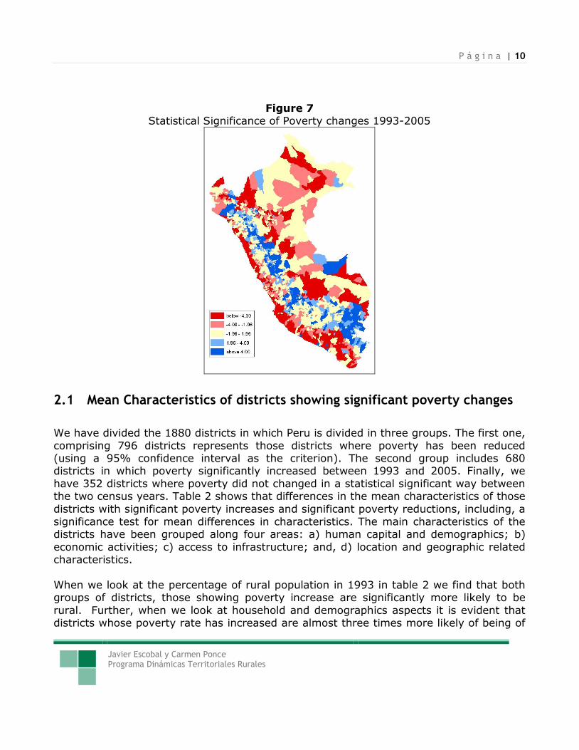
One way of assessing how important are the poverty changes depicted in Figure 6 is

show if these differences are statistically significant4. Figure 7 shows precisely this as an indicator of the statistical significance of poverty changes. Here it is again evident that poverty reductions along the Peruvian coastal areas are highly significant

4 We have calculate the statistical significance of poverty changes as follows: 2005 1993

1993

(0) (0)

. [ (0) ]

FGT FGTz

st dev FGT

P á g i n a | 10


Figure 7 Statistical Significance of Poverty changes 1993-2005

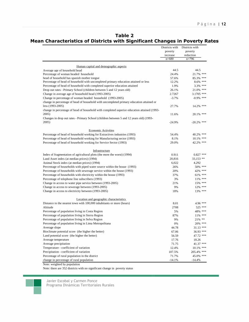
2.1 Mean Characteristics of districts showing significant poverty changes

We have divided the 1880 districts in which Peru is divided in three groups. The first one,

comprising 796 districts represents those districts where poverty has been reduced (using a 95% confidence interval as the criterion). The second group includes 680 districts in which poverty significantly increased between 1993 and 2005. Finally, we

have 352 districts where poverty did not changed in a statistical significant way between the two census years. Table 2 shows that differences in the mean characteristics of those

districts with significant poverty increases and significant poverty reductions, including, a significance test for mean differences in characteristics. The main characteristics of the districts have been grouped along four areas: a) human capital and demographics; b)

economic activities; c) access to infrastructure; and, d) location and geographic related characteristics.

When we look at the percentage of rural population in 1993 in table 2 we find that both groups of districts, those showing poverty increase are significantly more likely to be

rural. Further, when we look at household and demographics aspects it is evident that districts whose poverty rate has increased are almost three times more likely of being of

P á g i n a | 11


indigenous origin than those coming from district whose poverty rate got reduced. Similarly districts with poverty increase are those that have a significantly higher

proportion of female headed households5.

Educational differences are also apparent when we compared districts hose poverty rates have gone down and districts with increasing poverty rates. The first group has a lower percentage of head of households that have primary education or less and higher

percentage of head of households with higher education than the latter.

It is interesting to note that the type of economic activity in which households are involved is different for those that districts that have reduced poverty than those whose poverty rates have increased. This is especially clear in the rural districts where those

districts diversifying away from agriculture have been able to perform better.

Access to infrastructure is, of course key factors that differentiate those districts performing better in the 1993-2005 period as oppose to those that have increased their poverty rates. For the national aggregate and for the urban and rural segments of

sample is clear that those district having higher coverage of electricity, piped water and sewerage at the baseline (1993) where more likely to show a reduction in their poverty

rates. However, it is interesting to note that this pattern reverses when one looks at changes in service access (a proxy o investment in infrastructure services) areas.

Districts that have higher changes in access to piped water and electricity show poverty increases. This pattern may be capturing migration process as better endowed areas tend to increase their poverty rates if they received poor household migrating as a way

of improving their wellbeing

Location and geographic characteristics are also very different between those districts whose poverty got reduced between 1003 and 2005 and those that confronted a poverty increase. Besides those location variables already mentioned (being in a district from

Costa or Selva makes you more likely to observe a poverty reduction and being in a district from the Sierra region) ii is interesting to note that district that have lands with

lower slope tend to perform better. This is so even if bioclimatic potential may be worse-off or if precipitation is lower. Within rural areas, however, we can observe that better climate conditions do affect chances of been in a district that had a reduction in poverty.

5 We have also done the same exercise splitting the sample between those districts that are urban (50% or more of the population live in urban areas) or rural (50% or more of the population live in rural areas). The results are available upon request.

P á g i n a | 12


Districts with

poverty

increase

Districts with

poverty

reduction

n=680 n=796

Human capital and demographic aspects

Average age of household head 44.5 44.5

Percentage of woman headed household 24.4% 21.7% ***

head of household has spanish mother tongue 57.6% 85.3% ***

Percentage of head of household with uncompleted primary education attained or less 12.2% 8.6% ***

Percentage of head of household with completed superior education attained 1.9% 3.3% ***

Drop out rates - Primary School (children between 5 and 12 years old) 26.1% 21.0% ***

Change in average age of household head (1993-2005) 2.7267 3.1705 ***

Change in percentage of woman headed household (1993-2005) -3.7% -0.9% ***

change in percentage of head of household with uncompleted primary education attained or

less (1993-2005) 27.7% 14.2% ***

change in percentage of head of household with completed superior education attained (1993-

2005) 11.6% 20.1% ***

Changes in drop out rates - Primary School (children between 5 and 12 years old) (1993-

2005) -24.9% -20.2% ***

Economic Activities

Percentage of head of household working for Extractives industries (1993) 54.4% 40.2% ***

Percentage of head of household working for Manufacturing sector (1993) 8.1% 10.1% ***

Percentage of head of household working for Service Sector (1993) 29.0% 42.2% ***

Infrastructure

Index of fragmentation of agricultural plots (the more the worst) (1994) 0.911 0.827 ***

Land Asset index (at median prices) (1994) 20,816 33,153 **

Animal Stock index (at median prices) (1994) 6,022 4,292

Percentage of households with piped water source within the house (1993) 26% 50% ***

Percentage of households with sewerage service within the house (1993) 20% 42% ***

Percentage of households with electricity within the house (1993) 37% 61% ***

Percentage of telephone line subscribers (1993) 3% 11% ***

Change in access to water pipe service between (1993-2005) 21% 15% ***

Change in access to sewerage between (1993-2005) 9% 12% ***

Change in access to electricity between (1993-2005) 18% 13% ***

Location and geographic characteristics

Distance to the nearest town with 100,000 inhabitants or more (hours) 8.01 4.96 ***

Altitude 2708 525 ***

Percentage of population living in Costa Region 5% 48% ***

Percentage of population living in Sierra Region 87% 11% ***

Percentage of population living in Selva Region 9% 21% **

Percentage of population living in Lima Metropolitana 0% 20% ***

Average slope 44.78 31.13 ***

Bioclimate potential score (the higher the better) 67.06 36.93 ***

Land potential score (the higher the better) 56.59 47.72 ***

Average temperature 17.76 18.26

Average precipitation 71.75 41.37 ***

Temperature - coefficient of variation 12.4% 10.1% ***

Precipitation - coefficient of variation 107.5% 205.4% ***

Percentage of rural population in the district 71.7% 45.0% ***

change in percentage of rural population -14.1% -14.4%

Note: weighted by population

Note: there are 352 districts with no significant change in poverty status

Table 2 Mean Characteristics of Districts with Significant Changes in Poverty Rates

P á g i n a | 13


What has changed in Peru to explain such a change in poverty? A full explanation is

beyond the scope of this paper but it is clear that migration in a context of growth disparities should be at the core of any explanation6. As has been shown in World Bank

(2005), rural poverty has been most responsive to economic growth (1993-1997 and 2001-onwards) only in the Costa and least responsive in the Sierra. Further, in periods of stagnation (1997-2001) poverty in Rural and Selva regions has increased the most,

especially among those that are better linked to the product markets, the rest been able to buffer through increase in self-consumption.

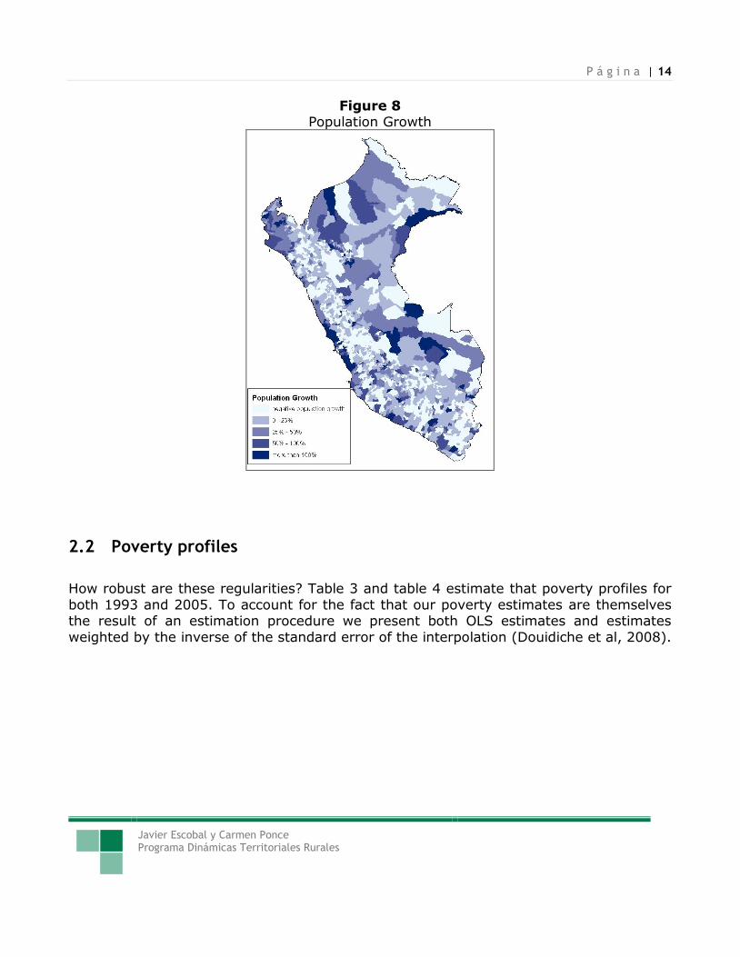
During this period, migration statistics are not readily available since migration related questions were not asked in the 2005 census. However population growth spatial

patterns are very clear as can be seen in Figure 8. Here we map population growth of all districts in Peru between 1993 and 2005. As can be seen in most of the Sierra region

population growth has been negative. Our results show that in those areas were population has grew the least or has diminished are areas where population has increased. This pattern is consistent with the fact that younger, better educated and

relatively more wealthy household are more capable to migrate, leaving behind older and less endowed households.

6 We have looked in detail to the methodology used to construct poverty lines in 1994 and 2005 to assure reasonably comparability. We noted the 1994 poverty lines for the Sierra included a slightly larger caloric intake than the one considered in 2006. Thus if any methodological bias exists go against blaming methodological differences as a way of explaining these poverty increases. On the contrary, poverty rates on the Sierra region may be slightly underestimated, which in turn will mean that poverty has increased marginally more than what we are estimating here. The study, however, does not incorporates this adjustment.

P á g i n a | 14


Figure 8 Population Growth

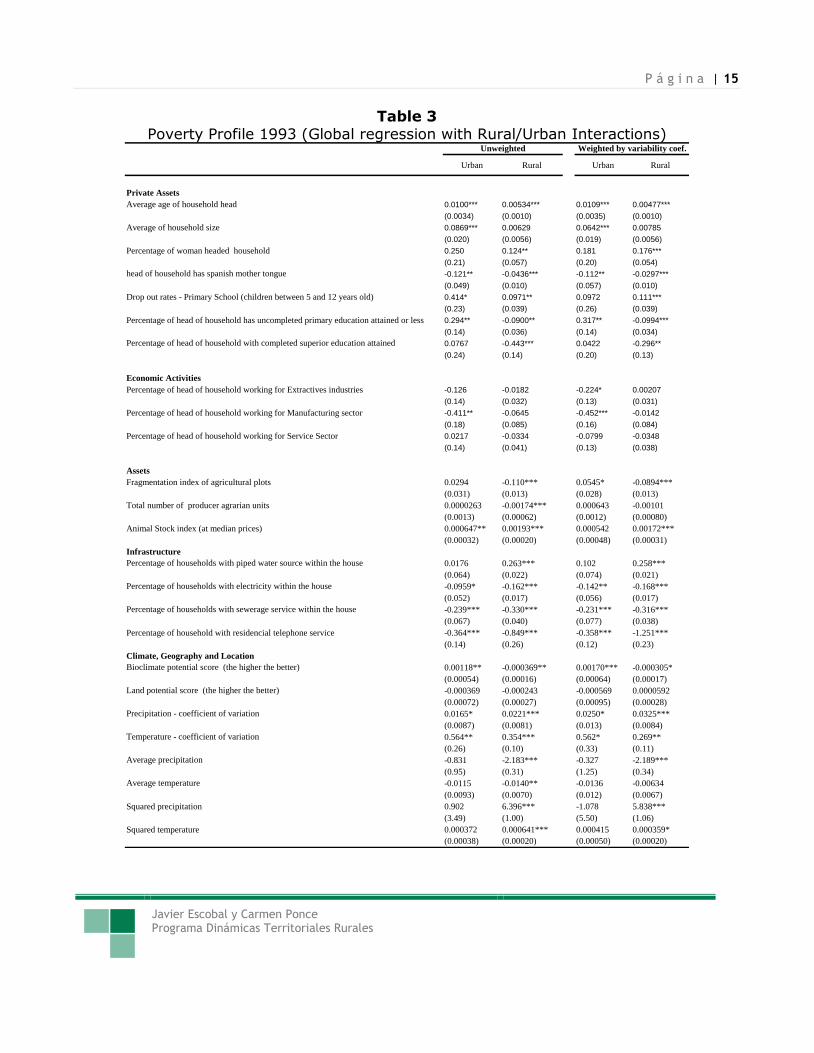
2.2 Poverty profiles

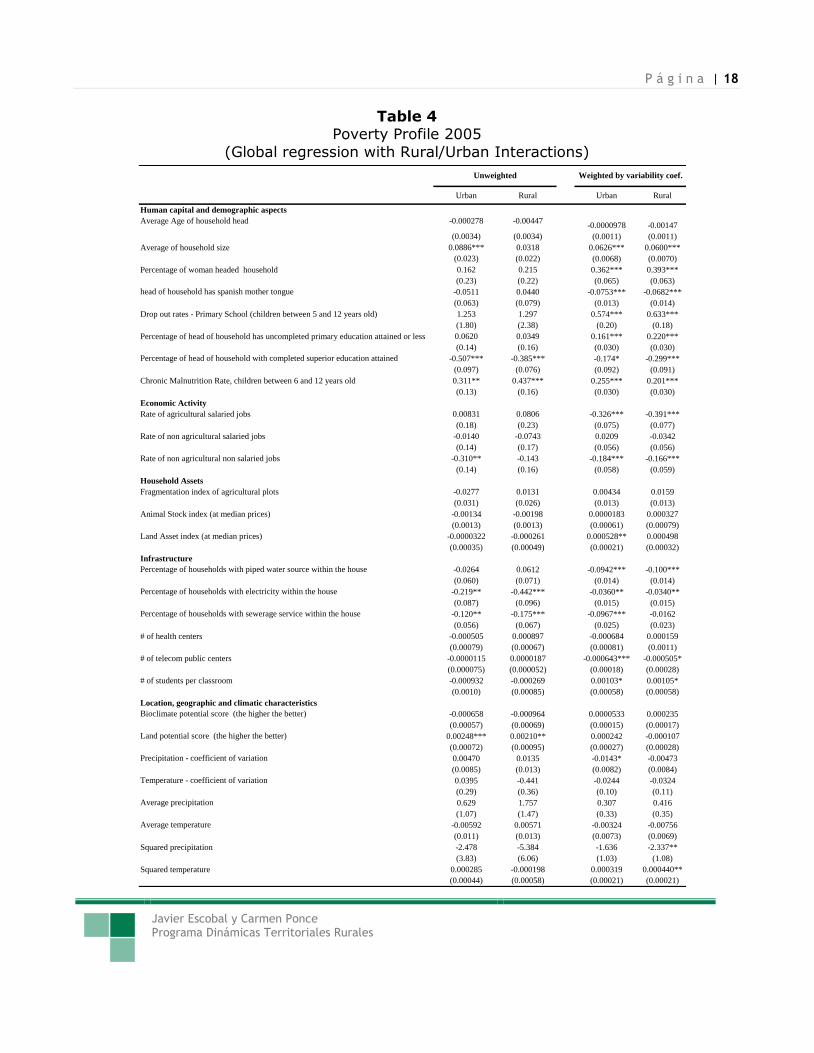
How robust are these regularities? Table 3 and table 4 estimate that poverty profiles for

both 1993 and 2005. To account for the fact that our poverty estimates are themselves the result of an estimation procedure we present both OLS estimates and estimates

weighted by the inverse of the standard error of the interpolation (Douidiche et al, 2008).

P á g i n a | 15


Table 3 Poverty Profile 1993 (Global regression with Rural/Urban Interactions)

Urban Rural Urban Rural

Private Assets

Average age of household head 0.0100*** 0.00534*** 0.0109*** 0.00477***

(0.0034) (0.0010) (0.0035) (0.0010)

Average of household size 0.0869*** 0.00629 0.0642*** 0.00785

(0.020) (0.0056) (0.019) (0.0056)

Percentage of woman headed household 0.250 0.124** 0.181 0.176***

(0.21) (0.057) (0.20) (0.054)

head of household has spanish mother tongue -0.121** -0.0436*** -0.112** -0.0297***

(0.049) (0.010) (0.057) (0.010)

Drop out rates - Primary School (children between 5 and 12 years old) 0.414* 0.0971** 0.0972 0.111***

(0.23) (0.039) (0.26) (0.039)

Percentage of head of household has uncompleted primary education attained or less 0.294** -0.0900** 0.317** -0.0994***

(0.14) (0.036) (0.14) (0.034)

Percentage of head of household with completed superior education attained 0.0767 -0.443*** 0.0422 -0.296**

(0.24) (0.14) (0.20) (0.13)

Economic Activities

Percentage of head of household working for Extractives industries -0.126 -0.0182 -0.224* 0.00207

(0.14) (0.032) (0.13) (0.031)

Percentage of head of household working for Manufacturing sector -0.411** -0.0645 -0.452*** -0.0142

(0.18) (0.085) (0.16) (0.084)

Percentage of head of household working for Service Sector 0.0217 -0.0334 -0.0799 -0.0348

(0.14) (0.041) (0.13) (0.038)

Assets

Fragmentation index of agricultural plots 0.0294 -0.110*** 0.0545* -0.0894***

(0.031) (0.013) (0.028) (0.013)

Total number of producer agrarian units 0.0000263 -0.00174*** 0.000643 -0.00101

(0.0013) (0.00062) (0.0012) (0.00080)

Animal Stock index (at median prices) 0.000647** 0.00193*** 0.000542 0.00172***

(0.00032) (0.00020) (0.00048) (0.00031)

Infrastructure

Percentage of households with piped water source within the house 0.0176 0.263*** 0.102 0.258***

(0.064) (0.022) (0.074) (0.021)

Percentage of households with electricity within the house -0.0959* -0.162*** -0.142** -0.168***

(0.052) (0.017) (0.056) (0.017)

Percentage of households with sewerage service within the house -0.239*** -0.330*** -0.231*** -0.316***

(0.067) (0.040) (0.077) (0.038)

Percentage of household with residencial telephone service -0.364*** -0.849*** -0.358*** -1.251***

(0.14) (0.26) (0.12) (0.23)

Climate, Geography and Location

Bioclimate potential score (the higher the better) 0.00118** -0.000369** 0.00170*** -0.000305*

(0.00054) (0.00016) (0.00064) (0.00017)

Land potential score (the higher the better) -0.000369 -0.000243 -0.000569 0.0000592

(0.00072) (0.00027) (0.00095) (0.00028)

Precipitation - coefficient of variation 0.0165* 0.0221*** 0.0250* 0.0325***

(0.0087) (0.0081) (0.013) (0.0084)

Temperature - coefficient of variation 0.564** 0.354*** 0.562* 0.269**

(0.26) (0.10) (0.33) (0.11)

Average precipitation -0.831 -2.183*** -0.327 -2.189***

(0.95) (0.31) (1.25) (0.34)

Average temperature -0.0115 -0.0140** -0.0136 -0.00634

(0.0093) (0.0070) (0.012) (0.0067)

Squared precipitation 0.902 6.396*** -1.078 5.838***

(3.49) (1.00) (5.50) (1.06)

Squared temperature 0.000372 0.000641*** 0.000415 0.000359*

(0.00038) (0.00020) (0.00050) (0.00020)

Unweighted Weighted by variability coef.

P á g i n a | 16


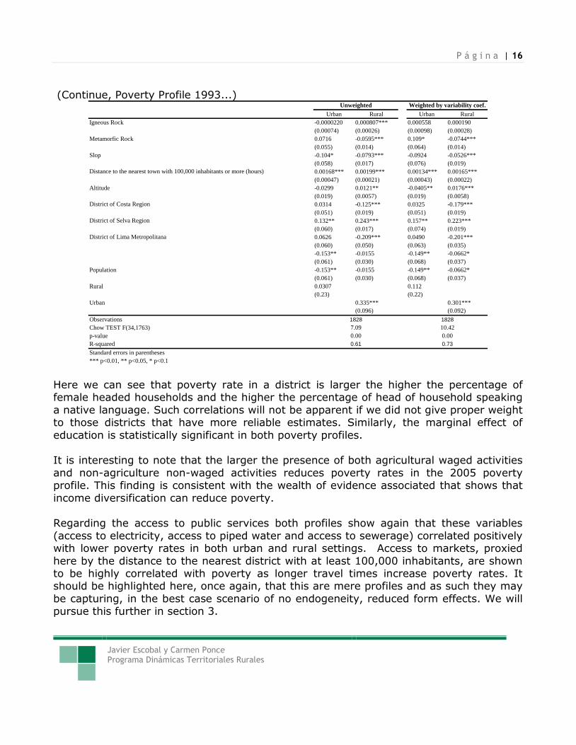
(Continue, Poverty Profile 1993...)


Igneous Rock -0.0000220 0.000807*** 0.000558 0.000190

(0.00074) (0.00026) (0.00098) (0.00028)

Metamorfic Rock 0.0716 -0.0595*** 0.109* -0.0744***

(0.055) (0.014) (0.064) (0.014)

Slop -0.104* -0.0793*** -0.0924 -0.0526***

(0.058) (0.017) (0.076) (0.019)

Distance to the nearest town with 100,000 inhabitants or more (hours) 0.00168*** 0.00199*** 0.00134*** 0.00165***

(0.00047) (0.00021) (0.00043) (0.00022)

Altitude -0.0299 0.0121** -0.0405** 0.0176***

(0.019) (0.0057) (0.019) (0.0058)

District of Costa Region 0.0314 -0.125*** 0.0325 -0.179***

(0.051) (0.019) (0.051) (0.019)

District of Selva Region 0.132** 0.243*** 0.157** 0.223***

(0.060) (0.017) (0.074) (0.019)

District of Lima Metropolitana 0.0626 -0.209*** 0.0490 -0.201***

(0.060) (0.050) (0.063) (0.035)

-0.153** -0.0155 -0.149** -0.0662*

(0.061) (0.030) (0.068) (0.037)

Population -0.153** -0.0155 -0.149** -0.0662*

(0.061) (0.030) (0.068) (0.037)

Rural 0.0307 0.112

(0.23) (0.22)

Urban 0.335*** 0.301***

(0.096) (0.092)

Observations

Chow TEST F(34,1763)

p-value

R-squared

Standard errors in parentheses

*** p<0.01, ** p<0.05, * p<0.1

0.61

1828

0.73

7.09 10.42

0.00 0.00

1828


Here we can see that poverty rate in a district is larger the higher the percentage of female headed households and the higher the percentage of head of household speaking

a native language. Such correlations will not be apparent if we did not give proper weight to those districts that have more reliable estimates. Similarly, the marginal effect of

education is statistically significant in both poverty profiles. It is interesting to note that the larger the presence of both agricultural waged activities

and non-agriculture non-waged activities reduces poverty rates in the 2005 poverty profile. This finding is consistent with the wealth of evidence associated that shows that

income diversification can reduce poverty. Regarding the access to public services both profiles show again that these variables

(access to electricity, access to piped water and access to sewerage) correlated positively with lower poverty rates in both urban and rural settings. Access to markets, proxied

here by the distance to the nearest district with at least 100,000 inhabitants, are shown to be highly correlated with poverty as longer travel times increase poverty rates. It should be highlighted here, once again, that this are mere profiles and as such they may

be capturing, in the best case scenario of no endogeneity, reduced form effects. We will pursue this further in section 3.

P á g i n a | 17


Finally, regarding other location and geographic correlates, they continue to be highly significant even if one controls by access to key private and public assets. For example,

altitude keeps correlating with higher poverty rates. Similarly, soil characteristics, and precipitation are variables that continue to be highly correlated with wellbeing outcomes.

P á g i n a | 18


Table 4 Poverty Profile 2005

(Global regression with Rural/Urban Interactions)


Human capital and demographic aspects

Average Age of household head -0.000278 -0.00447-0.0000978 -0.00147

(0.0034) (0.0034) (0.0011) (0.0011)

Average of household size 0.0886*** 0.0318 0.0626*** 0.0600***

(0.023) (0.022) (0.0068) (0.0070)

Percentage of woman headed household 0.162 0.215 0.362*** 0.393***

(0.23) (0.22) (0.065) (0.063)

head of household has spanish mother tongue -0.0511 0.0440 -0.0753*** -0.0682***

(0.063) (0.079) (0.013) (0.014)

Drop out rates - Primary School (children between 5 and 12 years old) 1.253 1.297 0.574*** 0.633***

(1.80) (2.38) (0.20) (0.18)

Percentage of head of household has uncompleted primary education attained or less 0.0620 0.0349 0.161*** 0.220***

(0.14) (0.16) (0.030) (0.030)

Percentage of head of household with completed superior education attained -0.507*** -0.385*** -0.174* -0.299***

(0.097) (0.076) (0.092) (0.091)

Chronic Malnutrition Rate, children between 6 and 12 years old 0.311** 0.437*** 0.255*** 0.201***

(0.13) (0.16) (0.030) (0.030)

Economic Activity

Rate of agricultural salaried jobs 0.00831 0.0806 -0.326*** -0.391***

(0.18) (0.23) (0.075) (0.077)

Rate of non agricultural salaried jobs -0.0140 -0.0743 0.0209 -0.0342

(0.14) (0.17) (0.056) (0.056)

Rate of non agricultural non salaried jobs -0.310** -0.143 -0.184*** -0.166***

(0.14) (0.16) (0.058) (0.059)

Household Assets

Fragmentation index of agricultural plots -0.0277 0.0131 0.00434 0.0159

(0.031) (0.026) (0.013) (0.013)

Animal Stock index (at median prices) -0.00134 -0.00198 0.0000183 0.000327

(0.0013) (0.0013) (0.00061) (0.00079)

Land Asset index (at median prices) -0.0000322 -0.000261 0.000528** 0.000498

(0.00035) (0.00049) (0.00021) (0.00032)

Infrastructure

Percentage of households with piped water source within the house -0.0264 0.0612 -0.0942*** -0.100***

(0.060) (0.071) (0.014) (0.014)

Percentage of households with electricity within the house -0.219** -0.442*** -0.0360** -0.0340**

(0.087) (0.096) (0.015) (0.015)

Percentage of households with sewerage service within the house -0.120** -0.175*** -0.0967*** -0.0162

(0.056) (0.067) (0.025) (0.023)

# of health centers -0.000505 0.000897 -0.000684 0.000159

(0.00079) (0.00067) (0.00081) (0.0011)

# of telecom public centers -0.0000115 0.0000187 -0.000643*** -0.000505*

(0.000075) (0.000052) (0.00018) (0.00028)

# of students per classroom -0.000932 -0.000269 0.00103* 0.00105*

(0.0010) (0.00085) (0.00058) (0.00058)

Location, geographic and climatic characteristics

Bioclimate potential score (the higher the better) -0.000658 -0.000964 0.0000533 0.000235

(0.00057) (0.00069) (0.00015) (0.00017)

Land potential score (the higher the better) 0.00248*** 0.00210** 0.000242 -0.000107

(0.00072) (0.00095) (0.00027) (0.00028)

Precipitation - coefficient of variation 0.00470 0.0135 -0.0143* -0.00473

(0.0085) (0.013) (0.0082) (0.0084)

Temperature - coefficient of variation 0.0395 -0.441 -0.0244 -0.0324

(0.29) (0.36) (0.10) (0.11)

Average precipitation 0.629 1.757 0.307 0.416

(1.07) (1.47) (0.33) (0.35)

Average temperature -0.00592 0.00571 -0.00324 -0.00756

(0.011) (0.013) (0.0073) (0.0069)

Squared precipitation -2.478 -5.384 -1.636 -2.337**

(3.83) (6.06) (1.03) (1.08)

Squared temperature 0.000285 -0.000198 0.000319 0.000440**

(0.00044) (0.00058) (0.00021) (0.00021)


P á g i n a | 19


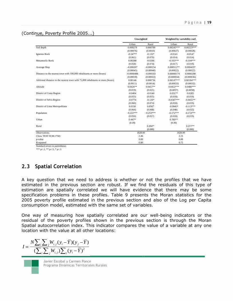
(Continue, Poverty Profile 2005...)


Soil depth 0.000279 0.000799 0.00245*** 0.00223***

(0.00076) (0.0010) (0.00027) (0.00028)

Igneous Rock -0.147** -0.132* -0.0141 -0.0147

(0.061) (0.070) (0.014) (0.014)

Metamorfic Rock 0.00288 -0.0266 -0.103*** -0.104***

(0.058) (0.074) (0.017) (0.019)

Average Slop -0.000207 -0.000154 0.000512** 0.000433*

(0.00045) (0.00040) (0.00022) (0.00022)

Distance to the nearest town with 100,000 inhabitants or more (hours) -0.0000488 -0.000103 0.00000174 0.0000298

(0.00018) (0.00022) (0.000034) (0.000036)

Aditional distance to the nearest town with 75,000 inhabitants or more (hours) 0.00146 0.000736 0.00147*** 0.00184***

(0.0011) (0.0014) (0.00033) (0.00032)

Altitude 0.0426** 0.0457** 0.0422*** 0.0480***

(0.019) (0.021) (0.0057) (0.0058)

District of Costa Region -0.0404 -0.0140 0.0317* 0.0283

(0.053) (0.055) (0.018) (0.019)

District of Selva Region -0.0774 -0.126* -0.0587*** -0.0455**

(0.060) (0.074) (0.018) (0.019)

District of Lima Metropolitana 0.0330 0.0567 -0.0945* -0.113***

(0.064) (0.068) (0.048) (0.033)

Population -0.222*** -0.253*** -0.172*** -0.172***

(0.050) (0.057) (0.018) (0.019)

Urban 0.447** 0.783***

(0.20) (0.20)

Rural 0.204** 0.277***

(0.099) (0.095)

Observations

Chow TEST F(38,1750)

p-value

R-squared

Standard errors in parentheses

*** p<.1, ** p<.5, * p<.1

0.80

1828.00

0.75

2.46 2.25

0.00 0.00

Unweighted

1828.00

Weighted by variability coef.

2.3 Spatial Correlation

A key question that we need to address is whether or not the profiles that we have estimated in the previous section are robust. If we find the residuals of this type of

estimation are spatially correlated we will have evidence that there may be some specification problems in these profiles. Table 9 presents the Moran statistics for the

2005 poverty profile estimated in the previous section and also of the Log per Capita consumption model, estimated with the same set of variables.

One way of measuring how spatially correlated are our well-being indicators or the residual of the poverty profiles shown in the previous section is through the Moran

Spatial autocorrelation index. This indicator compares the value of a variable at any one location with the value at all other locations:

,

2

,

( )( )

( ) ( )

i j i ji j

i j ii j i

N W y Y y YI

W y Y

P á g i n a | 20


(1)

where W represents some indicator of contiguity between observation i and j. For

example, in the simplest case if district j is adjacent to district i, Wij receives a weight of 1, and 0 otherwise. A Moran statistics closer to 1 indicates a bigger difference from the

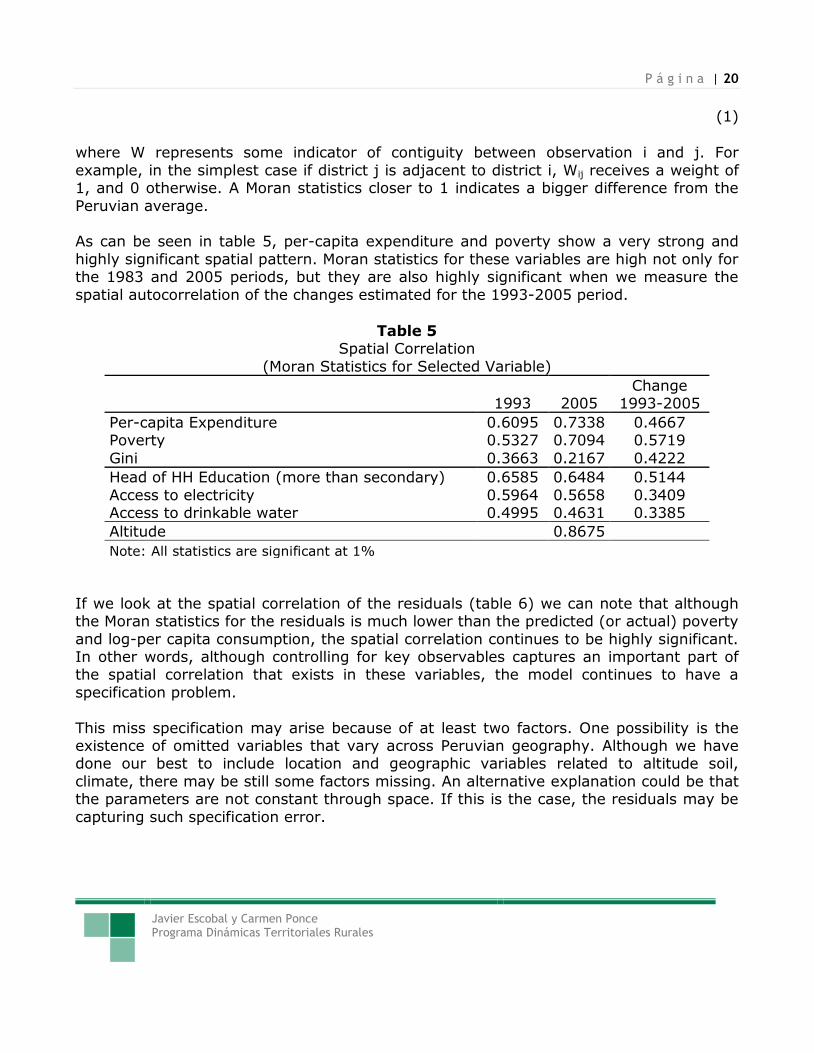
Peruvian average. As can be seen in table 5, per-capita expenditure and poverty show a very strong and

highly significant spatial pattern. Moran statistics for these variables are high not only for the 1983 and 2005 periods, but they are also highly significant when we measure the

spatial autocorrelation of the changes estimated for the 1993-2005 period.

Table 5 Spatial Correlation

(Moran Statistics for Selected Variable)

1993 2005 Change

1993-2005

Per-capita Expenditure 0.6095 0.7338 0.4667 Poverty 0.5327 0.7094 0.5719

Gini 0.3663 0.2167 0.4222

Head of HH Education (more than secondary) 0.6585 0.6484 0.5144

Access to electricity 0.5964 0.5658 0.3409 Access to drinkable water 0.4995 0.4631 0.3385

Altitude 0.8675

Note: All statistics are significant at 1%

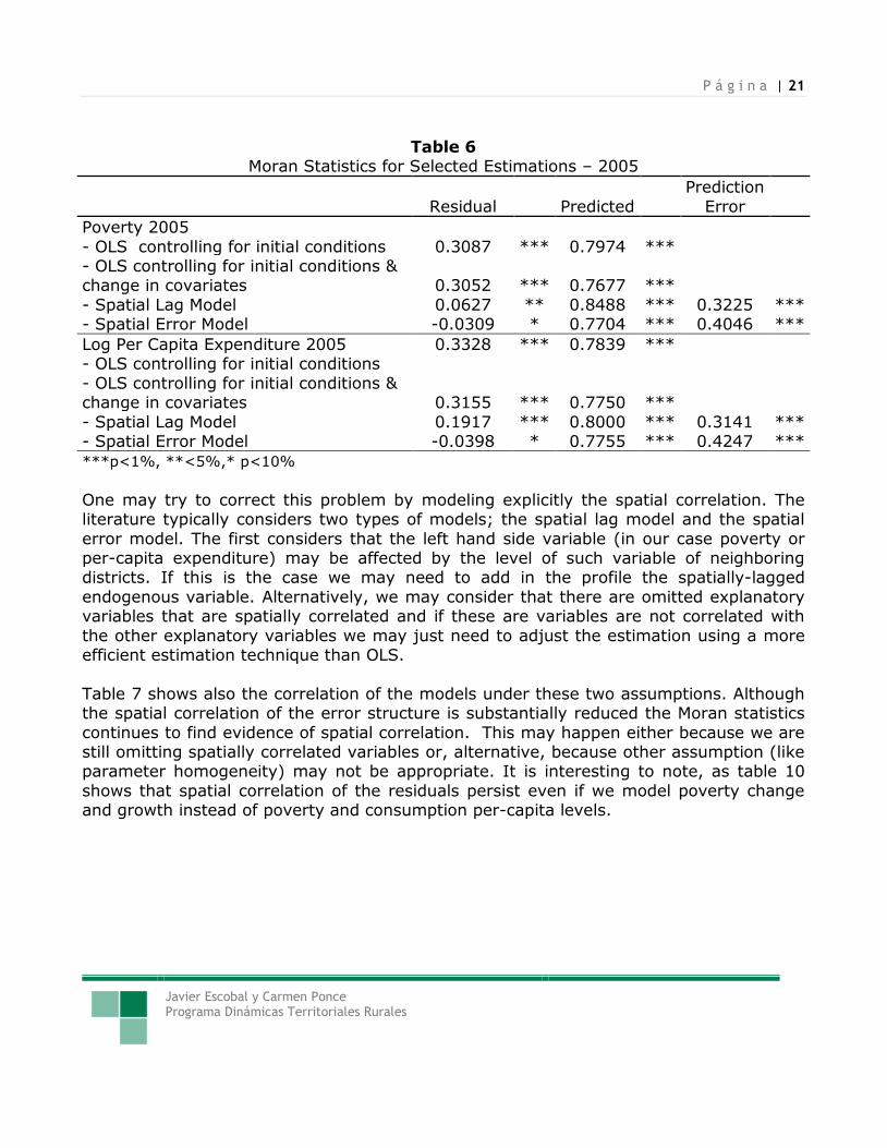
If we look at the spatial correlation of the residuals (table 6) we can note that although the Moran statistics for the residuals is much lower than the predicted (or actual) poverty

and log-per capita consumption, the spatial correlation continues to be highly significant. In other words, although controlling for key observables captures an important part of the spatial correlation that exists in these variables, the model continues to have a

specification problem.

This miss specification may arise because of at least two factors. One possibility is the existence of omitted variables that vary across Peruvian geography. Although we have done our best to include location and geographic variables related to altitude soil,

climate, there may be still some factors missing. An alternative explanation could be that the parameters are not constant through space. If this is the case, the residuals may be

capturing such specification error.

P á g i n a | 21


Table 6 Moran Statistics for Selected Estimations – 2005

Residual Predicted

Prediction

Error

Poverty 2005

- OLS controlling for initial conditions 0.3087 *** 0.7974 *** - OLS controlling for initial conditions & change in covariates 0.3052 *** 0.7677 ***

- Spatial Lag Model 0.0627 ** 0.8488 *** 0.3225 *** - Spatial Error Model -0.0309 * 0.7704 *** 0.4046 ***

Log Per Capita Expenditure 2005 0.3328 *** 0.7839 *** - OLS controlling for initial conditions

- OLS controlling for initial conditions & change in covariates 0.3155 *** 0.7750 ***

- Spatial Lag Model 0.1917 *** 0.8000 *** 0.3141 *** - Spatial Error Model -0.0398 * 0.7755 *** 0.4247 ***

***p<1%, **<5%,* p<10%

One may try to correct this problem by modeling explicitly the spatial correlation. The literature typically considers two types of models; the spatial lag model and the spatial

error model. The first considers that the left hand side variable (in our case poverty or per-capita expenditure) may be affected by the level of such variable of neighboring districts. If this is the case we may need to add in the profile the spatially-lagged

endogenous variable. Alternatively, we may consider that there are omitted explanatory variables that are spatially correlated and if these are variables are not correlated with

the other explanatory variables we may just need to adjust the estimation using a more efficient estimation technique than OLS.

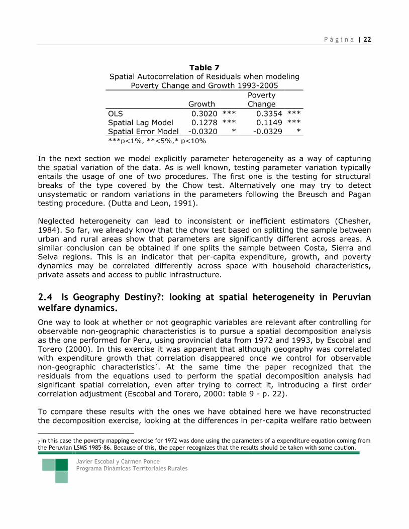
Table 7 shows also the correlation of the models under these two assumptions. Although the spatial correlation of the error structure is substantially reduced the Moran statistics

continues to find evidence of spatial correlation. This may happen either because we are still omitting spatially correlated variables or, alternative, because other assumption (like parameter homogeneity) may not be appropriate. It is interesting to note, as table 10

shows that spatial correlation of the residuals persist even if we model poverty change and growth instead of poverty and consumption per-capita levels.

P á g i n a | 22


Table 7 Spatial Autocorrelation of Residuals when modeling

Poverty Change and Growth 1993-2005

Growth Poverty Change

OLS 0.3020 *** 0.3354 *** Spatial Lag Model 0.1278 *** 0.1149 *** Spatial Error Model -0.0320 * -0.0329 *

***p<1%, **<5%,* p<10%

In the next section we model explicitly parameter heterogeneity as a way of capturing

the spatial variation of the data. As is well known, testing parameter variation typically entails the usage of one of two procedures. The first one is the testing for structural

breaks of the type covered by the Chow test. Alternatively one may try to detect unsystematic or random variations in the parameters following the Breusch and Pagan testing procedure. (Dutta and Leon, 1991).

Neglected heterogeneity can lead to inconsistent or inefficient estimators (Chesher,

1984). So far, we already know that the chow test based on splitting the sample between urban and rural areas show that parameters are significantly different across areas. A similar conclusion can be obtained if one splits the sample between Costa, Sierra and

Selva regions. This is an indicator that per-capita expenditure, growth, and poverty dynamics may be correlated differently across space with household characteristics,

private assets and access to public infrastructure.

2.4 Is Geography Destiny?: looking at spatial heterogeneity in Peruvian welfare dynamics.

One way to look at whether or not geographic variables are relevant after controlling for

observable non-geographic characteristics is to pursue a spatial decomposition analysis as the one performed for Peru, using provincial data from 1972 and 1993, by Escobal and

Torero (2000). In this exercise it was apparent that although geography was correlated with expenditure growth that correlation disappeared once we control for observable non-geographic characteristics7. At the same time the paper recognized that the

residuals from the equations used to perform the spatial decomposition analysis had significant spatial correlation, even after trying to correct it, introducing a first order

correlation adjustment (Escobal and Torero, 2000: table 9 - p. 22). To compare these results with the ones we have obtained here we have reconstructed

the decomposition exercise, looking at the differences in per-capita welfare ratio between

7 In this case the poverty mapping exercise for 1972 was done using the parameters of a expenditure equation coming from the Peruvian LSMS 1985-86. Because of this, the paper recognizes that the results should be taken with some caution.

P á g i n a | 23


the Sierra and Costa regions and between Selva and Costa regions8. The decomposition was done for both the 1993 and 2005 profiles and for the log-welfare-ratio differences (a

proxy of real expenditure growth).

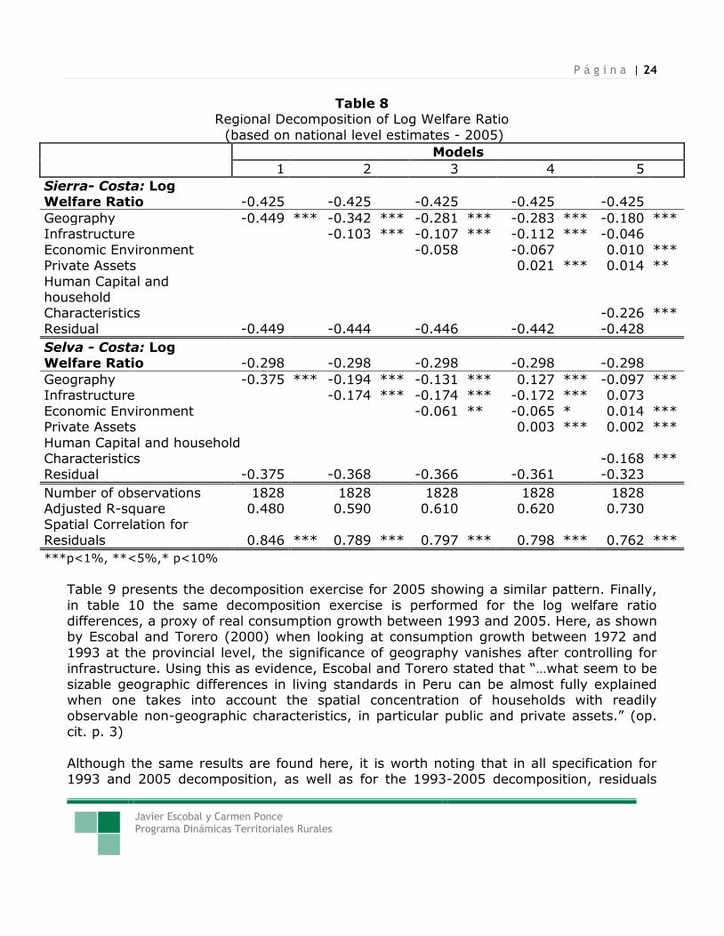
Table 8 presents the decomposition exercise for 1993 of estimated district level log welfare ratio differences between Sierra and Costa regions and between Selva and Costa regions. As can be seen here, geography remains an important factor correlated with log

welfare ratio differences even after sequentially controlling for infrastructure, economic environment, private assets and, finally, human capital and household characteristics.

These results are consistent with Escobal and Torero (2000). Further, the fact that spatial correlation of the residuals remains significant in all specification is also consistent with Escobal and Torero (2000) evidence.

8 The welfare ratio is constructed as that is the logarithm of per capita expenditure divided by the poverty line.

P á g i n a | 24


Table 8 Regional Decomposition of Log Welfare Ratio

(based on national level estimates - 2005)

Models

1 2 3 4 5

Sierra- Costa: Log Welfare Ratio -0.425 -0.425 -0.425 -0.425 -0.425

Geography -0.449 *** -0.342 *** -0.281 *** -0.283 *** -0.180 *** Infrastructure -0.103 *** -0.107 *** -0.112 *** -0.046

Economic Environment -0.058 -0.067 0.010 *** Private Assets 0.021 *** 0.014 **

Human Capital and household Characteristics -0.226 ***

Residual -0.449 -0.444 -0.446 -0.442 -0.428

Selva - Costa: Log Welfare Ratio -0.298 -0.298 -0.298 -0.298 -0.298

Geography -0.375 *** -0.194 *** -0.131 *** 0.127 *** -0.097 *** Infrastructure -0.174 *** -0.174 *** -0.172 *** 0.073

Economic Environment -0.061 ** -0.065 * 0.014 *** Private Assets 0.003 *** 0.002 ***

Human Capital and household Characteristics -0.168 *** Residual -0.375 -0.368 -0.366 -0.361 -0.323

Number of observations 1828 1828 1828 1828 1828 Adjusted R-square 0.480 0.590 0.610 0.620 0.730 Spatial Correlation for

Residuals 0.846 *** 0.789 *** 0.797 *** 0.798 *** 0.762 ***

***p<1%, **<5%,* p<10%

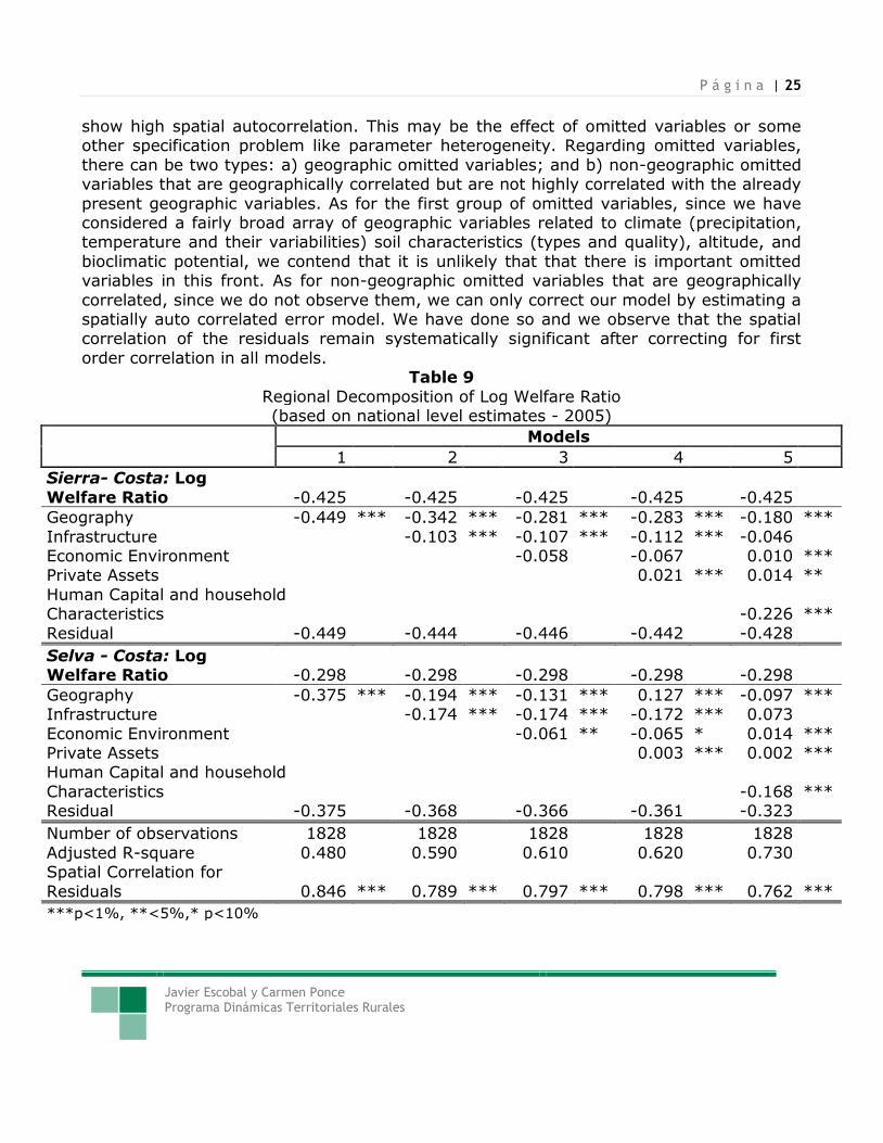
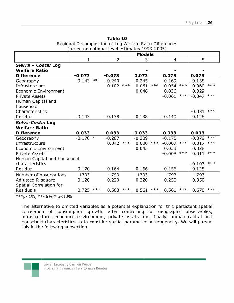
Table 9 presents the decomposition exercise for 2005 showing a similar pattern. Finally,

in table 10 the same decomposition exercise is performed for the log welfare ratio differences, a proxy of real consumption growth between 1993 and 2005. Here, as shown by Escobal and Torero (2000) when looking at consumption growth between 1972 and

1993 at the provincial level, the significance of geography vanishes after controlling for infrastructure. Using this as evidence, Escobal and Torero stated that “…what seem to be

sizable geographic differences in living standards in Peru can be almost fully explained when one takes into account the spatial concentration of households with readily observable non-geographic characteristics, in particular public and private assets.” (op.

cit. p. 3)

Although the same results are found here, it is worth noting that in all specification for 1993 and 2005 decomposition, as well as for the 1993-2005 decomposition, residuals

P á g i n a | 25


show high spatial autocorrelation. This may be the effect of omitted variables or some other specification problem like parameter heterogeneity. Regarding omitted variables,

there can be two types: a) geographic omitted variables; and b) non-geographic omitted variables that are geographically correlated but are not highly correlated with the already

present geographic variables. As for the first group of omitted variables, since we have considered a fairly broad array of geographic variables related to climate (precipitation, temperature and their variabilities) soil characteristics (types and quality), altitude, and

bioclimatic potential, we contend that it is unlikely that that there is important omitted variables in this front. As for non-geographic omitted variables that are geographically

correlated, since we do not observe them, we can only correct our model by estimating a spatially auto correlated error model. We have done so and we observe that the spatial correlation of the residuals remain systematically significant after correcting for first

order correlation in all models. Table 9

Regional Decomposition of Log Welfare Ratio (based on national level estimates - 2005)

Models

1 2 3 4 5

Sierra- Costa: Log

Welfare Ratio -0.425 -0.425 -0.425 -0.425 -0.425

Geography -0.449 *** -0.342 *** -0.281 *** -0.283 *** -0.180 ***

Infrastructure -0.103 *** -0.107 *** -0.112 *** -0.046 Economic Environment -0.058 -0.067 0.010 *** Private Assets 0.021 *** 0.014 **

Human Capital and household Characteristics -0.226 ***

Residual -0.449 -0.444 -0.446 -0.442 -0.428

Selva - Costa: Log Welfare Ratio -0.298 -0.298 -0.298 -0.298 -0.298

Geography -0.375 *** -0.194 *** -0.131 *** 0.127 *** -0.097 *** Infrastructure -0.174 *** -0.174 *** -0.172 *** 0.073

Economic Environment -0.061 ** -0.065 * 0.014 *** Private Assets 0.003 *** 0.002 *** Human Capital and household

Characteristics -0.168 *** Residual -0.375 -0.368 -0.366 -0.361 -0.323

Number of observations 1828 1828 1828 1828 1828

Adjusted R-square 0.480 0.590 0.610 0.620 0.730 Spatial Correlation for

Residuals 0.846 *** 0.789 *** 0.797 *** 0.798 *** 0.762 ***

***p<1%, **<5%,* p<10%

P á g i n a | 26


Table 10

Regional Decomposition of Log Welfare Ratio Differences (based on national level estimates 1993-2005)

Models

1 2 3 4 5

Sierra – Costa: Log

Welfare Ratio Difference -0.073 -0.073

-0.073

-0.073

-0.073

Geography -0.143 ** -0.240 -0.245 -0.169 -0.138 Infrastructure 0.102 *** 0.061 *** 0.054 *** 0.060 ***

Economic Environment 0.046 0.036 0.029 Private Assets -0.061 *** -0.047 *** Human Capital and

household Characteristics -0.031 ***

Residual -0.143 -0.138 -0.138 -0.140 -0.128

Selva-Costa: Log Welfare Ratio

Difference 0.033 0.033 0.033 0.033 0.033

Geography -0.170 * -0.207 -0.209 -0.175 -0.079 ***

Infrastructure 0.042 *** 0.000 *** -0.007 *** 0.017 *** Economic Environment 0.043 0.033 0.028 Private Assets -0.008 *** 0.011 ***

Human Capital and household characteristics -0.103 ***

Residual -0.170 -0.164 -0.166 -0.156 -0.125

Number of observations 1793 1793 1793 1793 1793 Adjusted R-square 0.120 0.220 0.220 0.250 0.350

Spatial Correlation for Residuals 0.725 *** 0.563 *** 0.561 *** 0.561 *** 0.670 ***

***p<1%, **<5%,* p<10%

The alternative to omitted variables as a potential explanation for this persistent spatial correlation of consumption growth, after controlling for geographic observables,

infrastructure, economic environment, private assets and, finally, human capital and household characteristics, is to consider spatial parameter heterogeneity. We will pursue

this in the following subsection.

P á g i n a | 27


2.5 Spatial heterogeneity: looking beyond the Global Model

An alternative to explore the importance of spatial factors in the dynamics of expenditure and poverty in Peru is to recognize that effect of private assets or the effect of the access

to public infrastructure are not constant throughout space. Spatial heterogeneity may arise may arise because environmental factors may operate differently at the local scale. It may also be the reflection of nonlinearities arising from complex. Minier, (2007) for

example, shows that parameter heterogeneity may be the reflection of local institutions.

There are different ways of modeling spatial parameter heterogeneity. We can explore other dimensions of heterogeneity in the parameter space by exploring parameter

variation across the welfare dimension through quantile regressions. Another way of exploring parameter heterogeneity is through spatially weighted regression, where local geographic-related parameters are estimated. Each of these ways of dealing with

parameter heterogeneity are based on different assumptions. For example, a quantile regression will assume that the relationship between the explanatory variables and the

consumption measure is the same in the different geographic spaces that share the observed attributes. Spatially weighted regression may be more flexible estimation but this is obtained, as we will see next, at the cost of parametrizing the way local

parameters behave. In this section, we will look at how these alternatives ways of recognizing parameter heterogeneity affect our conclusions.

Next we explore how this decomposition exercise may change if we allow parameters to change across the income distribution. To do this, we estimate our district level model

using quantile regressions for both urban and rural districts (where as before, rural districts are those that have the majority of the population located in rural towns). The

procedure followed here follows closely Nguyen et al (2007)9. We estimate the rates of return at each quantile and then we are able to construct a counterfactual distribution for the log welfare ratio assuming that rural households can hold the return of assets they

posses and received the average endowment that their urban counterparts in the same quintile posses.

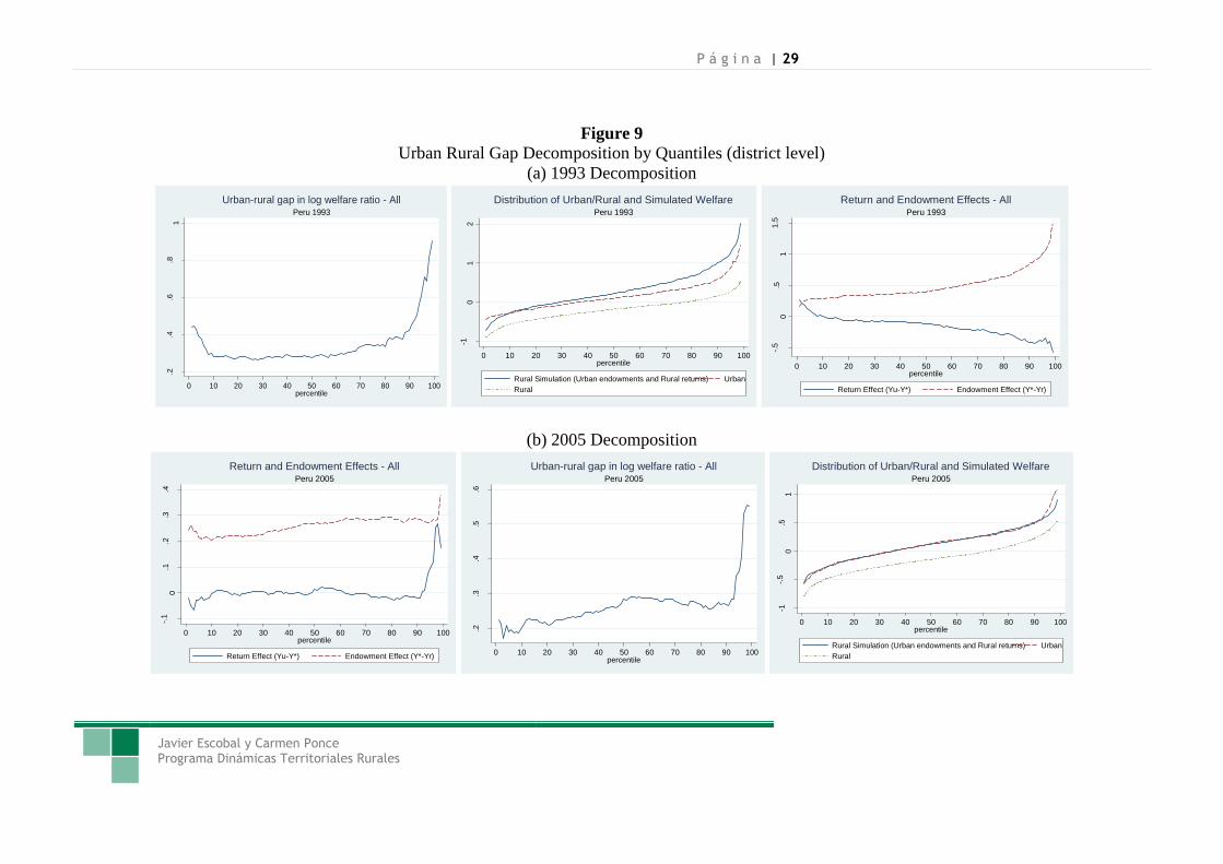
The first graph in panel (a) in figure 9 depicts the urban gap for the log welfare ratio for 1993. The next graph in the same panel shows the urban and rural log welfare ratio

wage for all quantiles, as well as the counterfactual distribution that mimics what the rural log welfare ratio will be if rural household had access to the asset endowment of

their urban counterpart. Finally the third graph in panel (a) graph the decomposition of the log welfare ratio across quintiles between the effect of differences in returns and

9 A detailed analysis using quantile regressions to decompose the urban rural wellbeing gap can be found in Escobal and Ponce (2008).

P á g i n a | 28


differences in asset endowments. As can be seen here the counterfactual curve rises above the urban curve for all quintiles except for the bottom 10%, indicating that rates

of return to assets are larger in urban than in rural areas for most of the expenditure distribution range. Further, the decomposition exercise shows that contribution of the

asset endowment in explaining the urban rural log-welfare gap increases steadily through all quintiles, while the contribution of having larger returns in the rural area decreases steadily as well.

Panel (b) in figure 9 shows the three same graphs for 2005. They show a similar pattern

to the one observed in 1993 with one interesting difference: the counterfactual curve does not rise above the urban curve, indicating that the marginal returns to assets in rural areas in 2005 are no longer above the marginal return to assets in urban areas

throughout all quintiles.

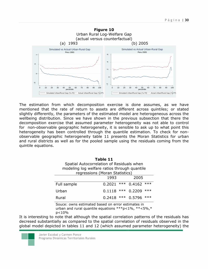
Figure 10 compares the actual urban/rural log welfare ratio gap with the one obtained from the counterfactual distribution (with rural households having the same endowment base than the average of the corresponding urban quintile for both the district level

estimates based on both interpolations (1993 and 2005). We can confirm here that the gap will be much lower if asset distribution was biased against rural dwellers and that

this is so across all of the quintile distribution. In addition the increase in rate of returns to endowments in urban areas and the reduction in the rate of returns to endowments in

rural areas (specially in the sierra) have made that the urban/rural log welfare ratio gap depends now more than before on the unequal distribution of assets between regions.

P á g i n a | 29


Figure 9

Urban Rural Gap Decomposition by Quantiles (district level)

(a) 1993 Decomposition .2

.4.6

.81

log

(u

rba

n w

.r./ru

ral w

.r.)

0 10 20 30 40 50 60 70 80 90 100percentile

Peru 1993

Urban-rural gap in log welfare ratio - All

-10

12

log

welfa

re r

atio

0 10 20 30 40 50 60 70 80 90 100percentile

Rural Simulation (Urban endowments and Rural returns) Urban

Rural

Peru 1993

Distribution of Urban/Rural and Simulated Welfare

-.5

0.5

11

.5

Diffe

ren

ce in

log

welfa

re r

atio

0 10 20 30 40 50 60 70 80 90 100percentile

Return Effect (Yu-Y*) Endowment Effect (Y*-Yr)

Peru 1993

Return and Endowment Effects - All

(b) 2005 Decomposition

-.1

0.1

.2.3

.4

Diffe

ren

ce in

log

welfa

re r

atio

0 10 20 30 40 50 60 70 80 90 100percentile

Return Effect (Yu-Y*) Endowment Effect (Y*-Yr)

Peru 2005

Return and Endowment Effects - All.2

.3.4

.5.6

log

(u

rba

n w

.r./ru

ral w

.r.)

0 10 20 30 40 50 60 70 80 90 100percentile

Peru 2005

Urban-rural gap in log welfare ratio - All

-1-.

50

.51

log

welfa

re r

atio

0 10 20 30 40 50 60 70 80 90 100percentile

Rural Simulation (Urban endowments and Rural returns) Urban

Rural

Peru 2005

Distribution of Urban/Rural and Simulated Welfare

P á g i n a | 30


Figure 10 Urban Rural Log-Welfare Gap

(actual versus counterfactual) (a) 1993 (b) 2005

-.5

0.5

1

Diffe

ren

ce in

log

welfa

re r

atio

0 10 20 30 40 50 60 70 80 90 100percentile

Simulated Urban/Rural Gap (Yu-Yr) Actual Urban/Rural Gap (Yu-Y*)

Peru 1993

Simulated vs Actual Urban-Rural Gap

-.2

0.2

.4.6

Diffe

ren

ce in

log

welfa

re r

atio

0 10 20 30 40 50 60 70 80 90 100percentile

Simulated Urban/Rural Gap (Yu-Yr) Actual Urban/Rural Gap (Yu-Y*)

Peru 2005

Simulated vs Actual Urban-Rural Gap

The estimation from which decomposition exercise is done assumes, as we have mentioned that the rate of return to assets are different across quintiles; or stated

slightly differently, the parameters of the estimated model are heterogeneous across the wellbeing distribution. Since we have shown in the previous subsection that there the decomposition exercise that assumed parameter heterogeneity was not able to control

for non-observable geographic heterogeneity, it is sensible to ask up to what point this heterogeneity has been controlled through the quantile estimation. To check for non-

observable geographic heterogeneity table 11 presents the Moran Statistics for urban and rural districts as well as for the pooled sample using the residuals coming from the

quintile equations.

Table 11

Spatial Autocorrelation of Residuals when modeling log welfare ratios through quantile

regressions (Moran Statistics)

1993 2005

Full sample 0.2021 *** 0.4162 ***

Urban 0.1118 *** 0.2209 ***

Rural 0.2418 *** 0.5796 ***

Souce: owns estimated based on error estimates in

urban and rural quantile equations ***p<1%, **<5%,*

p<10%

It is interesting to note that although the spatial correlation patterns of the residuals has

decresed substantially as compared to the spatial correlation of residuals observed in the global model depicted in tables 11 and 12 (which assumed parameter heterogeneity) the

P á g i n a | 31


spatial correlation is still highly significant. That is even if quantile regressions may be capturing some of the rate of return heterogeneity that is present in the sample, we still

must recognize that welfare differences have persistence spatial characteristics, that cannot be fully accounted by observables characteristics including the most common

geographic variables, infrastructure, economic environment, private assets and, finally, human capital and household characteristics. This fact remains true even if we recognize that rate of returns to assets are different between urban and rural sector and between

the poor and less poor. To explore further this issue we will look next at yet another way of parameterize the spatial heterogeneity of the rate of return in urban and rural Peru.

Capturing Local Spatial heterogeneity by estimating spatially weighted regressions

To capture this spatial heterogeneity we have re-estimated our global profile allowing for

parameter heterogeneity using a geographic weighted regression technique. Thus, instead of estimating:

0

1

k

i i

i

y x (2)

we estimate the following model:

1 2 0 1 2 1 2 1 2

1

( , ) ( , ) ( , ) ( , )k

i i

i

y l l l l l l x l l (3)

where l1 y l2 represent the location – longitude and latitude – of each observation.

Following Brunsdon et al.(2008) the parameters can be estimates using geographically weighted least squares (gwr) using the following weighting structure:

1

1 2 1 2 1 2( , ) ( , ) ( , )l l X W l l X X W l l Y (4)

The weights are chosen in such a way that the observations that are near to the point were the local parameter is estimated have more influence in the estimation than

observations that are far apart. If we use a Gaussian weighting function, the weight for the i-th observation will look as follows:

2

1 2( , ) exp /iw l l d h (5)

where d is the distance between the i-th observation and local point (l1,l2) in which the parameter is estimated. h reflects the bandwidth, that is the area where observation do

influence the local estimation. Thus the parameter estimated is basically a local

P á g i n a | 32


interpolation in which closest observation (within the bandwidth) have greater influence in the way changes in private and public assets affect per-capita expenditure or poverty.

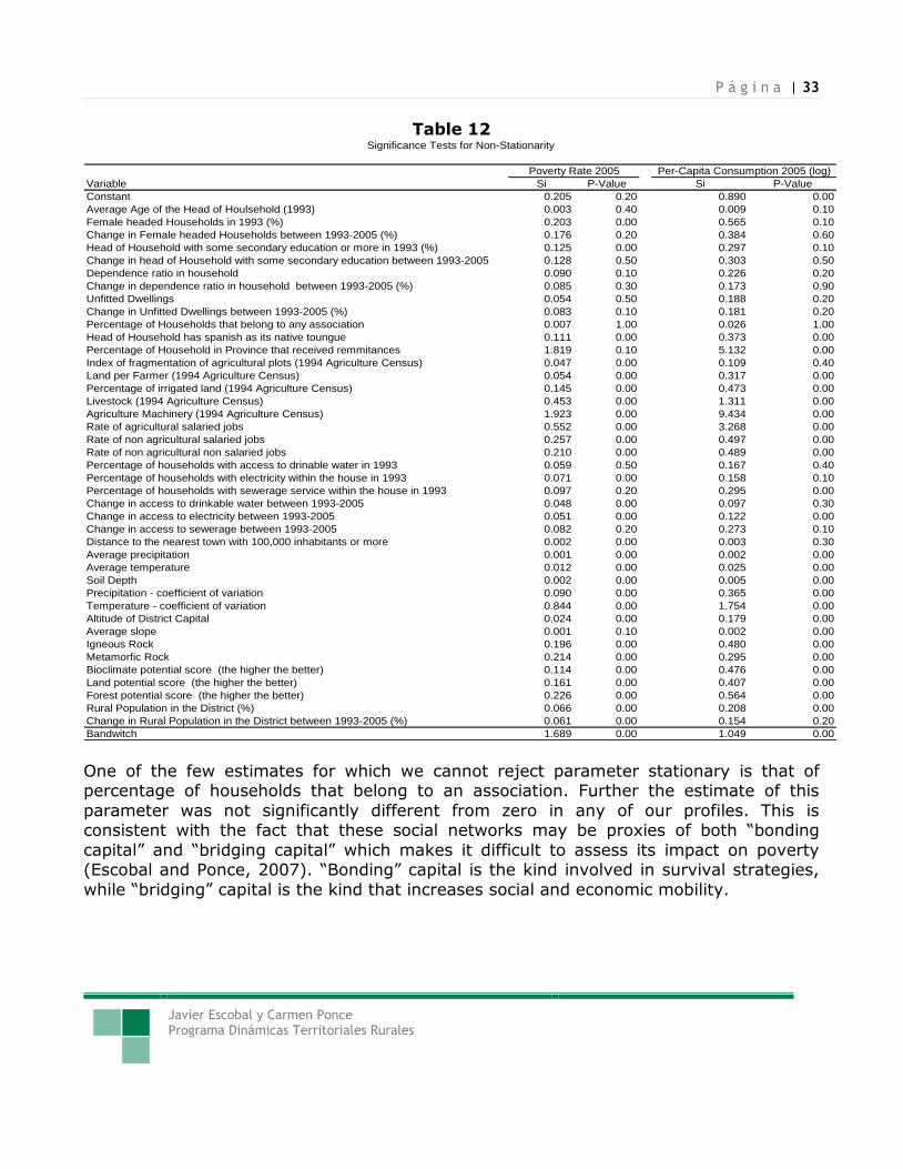
Table 12 shows the values and significance levels for the non-stationarity tests for both

the 2005 poverty and per-capita expenditure profiles. These tests are based on Monte Carlo simulations to evaluate whether the spatial variations in the parameter estimates are simple due to random variation or are effective spatial patterns. The tests show

clearly that for most of the right-hand side variables the spatial variation is highly statistically significant. For example, both the effects of initial levels of access to

electricity and access increase between 1993 and 2005 have significant variation over time. Wit respect to household characteristics, the role of education, the effect of female headed households or the effect of ethnicity also varies spatially when we correlate these

variables either with poverty or log per-capita expenditures. Finally, as was expected the impact of all location and geographic related variables changes across space.

P á g i n a | 33


Table 12

Variable Si P-Value Si P-Value

Constant 0.205 0.20 0.890 0.00

Average Age of the Head of Houlsehold (1993) 0.003 0.40 0.009 0.10

Female headed Households in 1993 (%) 0.203 0.00 0.565 0.10

Change in Female headed Households between 1993-2005 (%) 0.176 0.20 0.384 0.60

Head of Household with some secondary education or more in 1993 (%) 0.125 0.00 0.297 0.10

Change in head of Household with some secondary education between 1993-2005 0.128 0.50 0.303 0.50

Dependence ratio in household 0.090 0.10 0.226 0.20

Change in dependence ratio in household between 1993-2005 (%) 0.085 0.30 0.173 0.90

Unfitted Dwellings 0.054 0.50 0.188 0.20

Change in Unfitted Dwellings between 1993-2005 (%) 0.083 0.10 0.181 0.20

Percentage of Households that belong to any association 0.007 1.00 0.026 1.00

Head of Household has spanish as its native toungue 0.111 0.00 0.373 0.00

Percentage of Household in Province that received remmitances 1.819 0.10 5.132 0.00

Index of fragmentation of agricultural plots (1994 Agriculture Census) 0.047 0.00 0.109 0.40

Land per Farmer (1994 Agriculture Census) 0.054 0.00 0.317 0.00

Percentage of irrigated land (1994 Agriculture Census) 0.145 0.00 0.473 0.00

Livestock (1994 Agriculture Census) 0.453 0.00 1.311 0.00

Agriculture Machinery (1994 Agriculture Census) 1.923 0.00 9.434 0.00

Rate of agricultural salaried jobs 0.552 0.00 3.268 0.00

Rate of non agricultural salaried jobs 0.257 0.00 0.497 0.00

Rate of non agricultural non salaried jobs 0.210 0.00 0.489 0.00

Percentage of households with access to drinable water in 1993 0.059 0.50 0.167 0.40

Percentage of households with electricity within the house in 1993 0.071 0.00 0.158 0.10

Percentage of households with sewerage service within the house in 1993 0.097 0.20 0.295 0.00

Change in access to drinkable water between 1993-2005 0.048 0.00 0.097 0.30

Change in access to electricity between 1993-2005 0.051 0.00 0.122 0.00

Change in access to sewerage between 1993-2005 0.082 0.20 0.273 0.10

Distance to the nearest town with 100,000 inhabitants or more 0.002 0.00 0.003 0.30

Average precipitation 0.001 0.00 0.002 0.00

Average temperature 0.012 0.00 0.025 0.00

Soil Depth 0.002 0.00 0.005 0.00

Precipitation - coefficient of variation 0.090 0.00 0.365 0.00

Temperature - coefficient of variation 0.844 0.00 1.754 0.00

Altitude of District Capital 0.024 0.00 0.179 0.00

Average slope 0.001 0.10 0.002 0.00

Igneous Rock 0.196 0.00 0.480 0.00

Metamorfic Rock 0.214 0.00 0.295 0.00

Bioclimate potential score (the higher the better) 0.114 0.00 0.476 0.00

Land potential score (the higher the better) 0.161 0.00 0.407 0.00

Forest potential score (the higher the better) 0.226 0.00 0.564 0.00

Rural Population in the District (%) 0.066 0.00 0.208 0.00

Change in Rural Population in the District between 1993-2005 (%) 0.061 0.00 0.154 0.20

Bandwitch 1.689 0.00 1.049 0.00

Significance Tests for Non-Stationarity

Poverty Rate 2005 Per-Capita Consumption 2005 (log)

One of the few estimates for which we cannot reject parameter stationary is that of percentage of households that belong to an association. Further the estimate of this

parameter was not significantly different from zero in any of our profiles. This is consistent with the fact that these social networks may be proxies of both “bonding

capital” and “bridging capital” which makes it difficult to assess its impact on poverty (Escobal and Ponce, 2007). “Bonding” capital is the kind involved in survival strategies,

while “bridging” capital is the kind that increases social and economic mobility.

P á g i n a | 34


Another way of testing parameter heterogeneity is to look at the significance test for the bandwidth. The test is highly significant for both models (bandwidths of 1.6892 and

1.0487 for the poverty and log expenditure models, respectively, being both values significant at the 99% level).

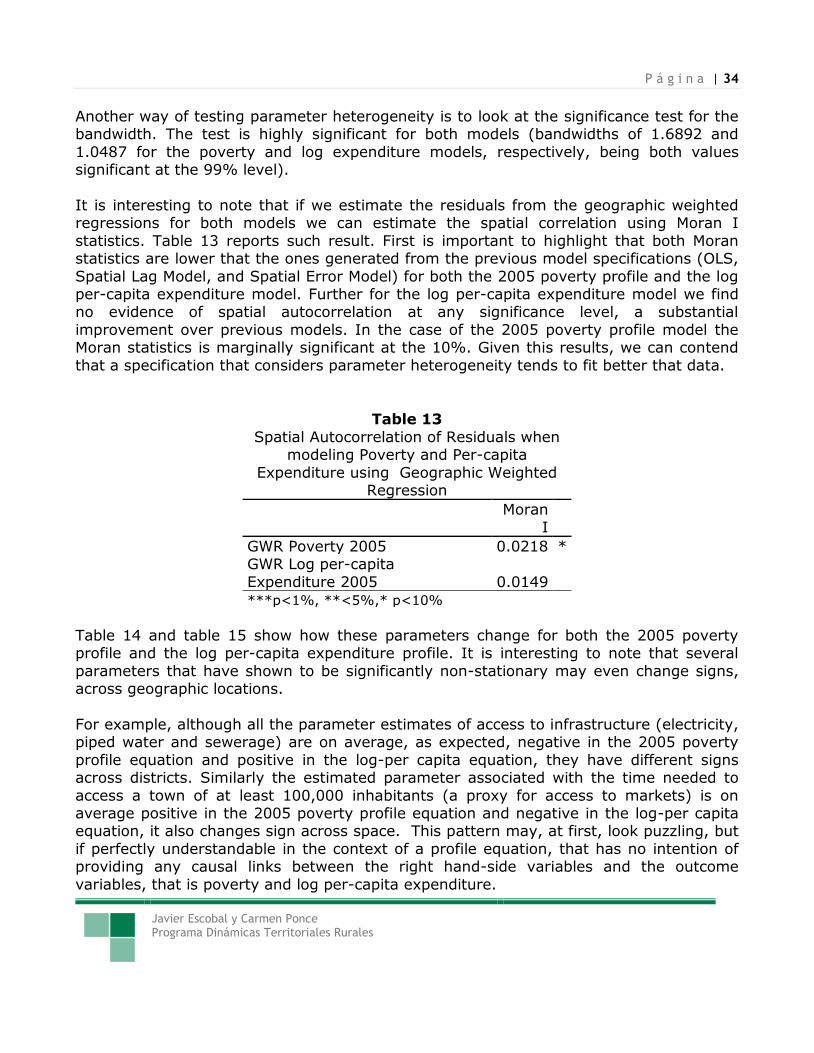
It is interesting to note that if we estimate the residuals from the geographic weighted regressions for both models we can estimate the spatial correlation using Moran I

statistics. Table 13 reports such result. First is important to highlight that both Moran statistics are lower that the ones generated from the previous model specifications (OLS,

Spatial Lag Model, and Spatial Error Model) for both the 2005 poverty profile and the log per-capita expenditure model. Further for the log per-capita expenditure model we find no evidence of spatial autocorrelation at any significance level, a substantial

improvement over previous models. In the case of the 2005 poverty profile model the Moran statistics is marginally significant at the 10%. Given this results, we can contend

that a specification that considers parameter heterogeneity tends to fit better that data.

Table 13

Spatial Autocorrelation of Residuals when modeling Poverty and Per-capita

Expenditure using Geographic Weighted Regression

Moran

I

GWR Poverty 2005 0.0218 * GWR Log per-capita

Expenditure 2005 0.0149

***p<1%, **<5%,* p<10%

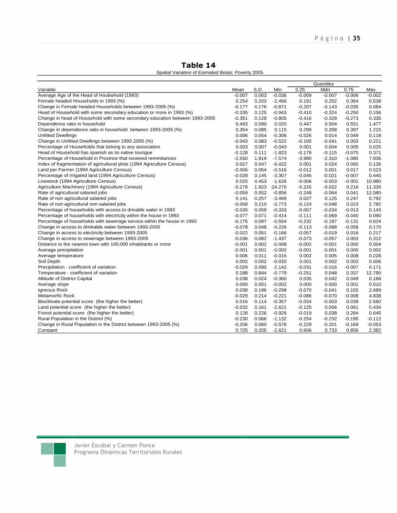
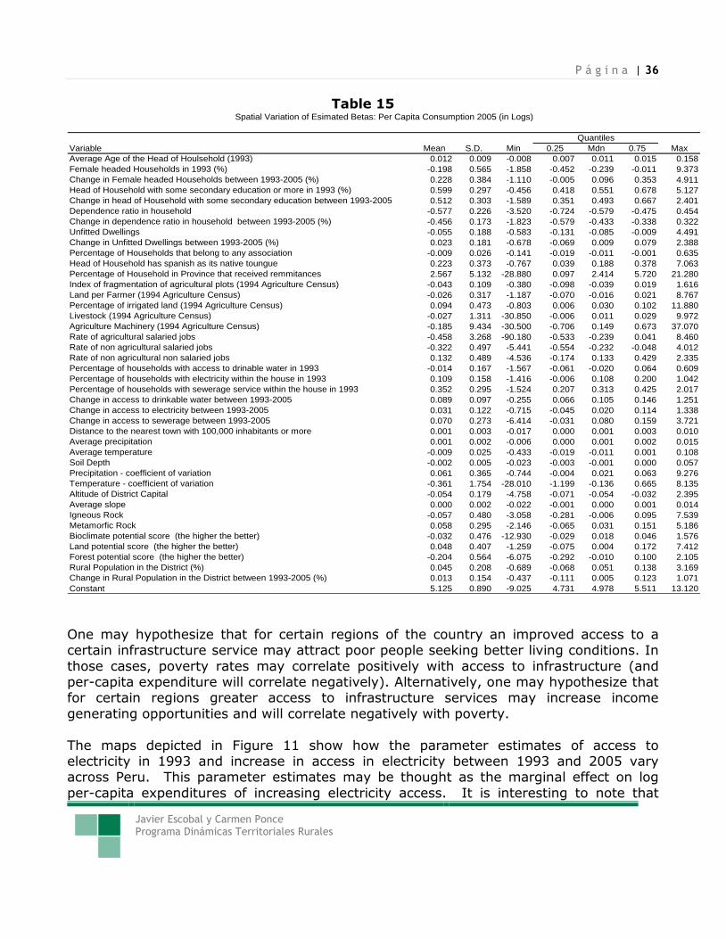
Table 14 and table 15 show how these parameters change for both the 2005 poverty profile and the log per-capita expenditure profile. It is interesting to note that several

parameters that have shown to be significantly non-stationary may even change signs, across geographic locations.

For example, although all the parameter estimates of access to infrastructure (electricity, piped water and sewerage) are on average, as expected, negative in the 2005 poverty

profile equation and positive in the log-per capita equation, they have different signs across districts. Similarly the estimated parameter associated with the time needed to

access a town of at least 100,000 inhabitants (a proxy for access to markets) is on average positive in the 2005 poverty profile equation and negative in the log-per capita equation, it also changes sign across space. This pattern may, at first, look puzzling, but

if perfectly understandable in the context of a profile equation, that has no intention of providing any causal links between the right hand-side variables and the outcome

variables, that is poverty and log per-capita expenditure.

P á g i n a | 35


Table 14

Variable Mean S.D. Min 0.25 Mdn 0.75 Max

Average Age of the Head of Houlsehold (1993) -0.007 0.003 -0.036 -0.009 -0.007 -0.006 -0.002

Female headed Households in 1993 (%) 0.254 0.203 -2.456 0.191 0.252 0.364 0.538

Change in Female headed Households between 1993-2005 (%) -0.177 0.176 -0.871 -0.267 -0.143 -0.035 0.084

Head of Household with some secondary education or more in 1993 (%) -0.335 0.125 -0.943 -0.410 -0.324 -0.250 0.106

Change in head of Household with some secondary education between 1993-2005 -0.351 0.128 -0.805 -0.416 -0.328 -0.273 0.335

Dependence ratio in household 0.493 0.090 0.020 0.447 0.504 0.551 1.477

Change in dependence ratio in household between 1993-2005 (%) 0.354 0.085 0.115 0.299 0.358 0.397 1.215

Unfitted Dwellings 0.006 0.054 -0.306 -0.026 0.014 0.049 0.118

Change in Unfitted Dwellings between 1993-2005 (%) -0.043 0.083 -0.522 -0.100 -0.041 0.003 0.221

Percentage of Households that belong to any association 0.003 0.007 -0.043 0.001 0.004 0.005 0.025

Head of Household has spanish as its native toungue -0.128 0.111 -1.823 -0.179 -0.115 -0.075 0.371

Percentage of Household in Province that received remmitances -2.550 1.819 -7.574 -3.980 -2.310 -1.080 7.936

Index of fragmentation of agricultural plots (1994 Agriculture Census) 0.027 0.047 -0.422 0.001 0.024 0.065 0.136

Land per Farmer (1994 Agriculture Census) -0.006 0.054 -0.516 -0.012 0.001 0.017 0.523

Percentage of irrigated land (1994 Agriculture Census) -0.028 0.145 -3.307 -0.045 -0.021 -0.007 0.445

Livestock (1994 Agriculture Census) 0.025 0.453 -1.626 -0.006 -0.003 -0.001 10.980

Agriculture Machinery (1994 Agriculture Census) -0.278 1.923 -24.270 -0.225 -0.022 0.218 11.330

Rate of agricultural salaried jobs -0.059 0.552 -0.856 -0.248 -0.064 0.041 12.580

Rate of non agricultural salaried jobs 0.141 0.257 -3.499 0.027 0.125 0.247 0.792

Rate of non agricultural non salaried jobs -0.058 0.210 -0.773 -0.124 -0.048 0.023 2.782

Percentage of households with access to drinable water in 1993 -0.035 0.059 -0.333 -0.057 -0.034 -0.013 0.143

Percentage of households with electricity within the house in 1993 -0.077 0.071 -0.414 -0.111 -0.069 -0.040 0.090

Percentage of households with sewerage service within the house in 1993 -0.175 0.097 -0.554 -0.232 -0.187 -0.131 0.624

Change in access to drinkable water between 1993-2005 -0.078 0.048 -0.226 -0.113 -0.088 -0.058 0.170

Change in access to electricity between 1993-2005 -0.022 0.051 -0.166 -0.057 -0.019 0.016 0.217

Change in access to sewerage between 1993-2005 -0.036 0.082 -1.437 -0.073 -0.057 0.003 0.312

Distance to the nearest town with 100,000 inhabitants or more -0.001 0.002 -0.008 -0.002 -0.001 0.000 0.004

Average precipitation -0.001 0.001 -0.002 -0.001 -0.001 0.000 0.002

Average temperature 0.006 0.011 -0.015 0.002 0.005 0.008 0.228

Soil Depth 0.002 0.002 -0.020 0.001 0.002 0.003 0.006

Precipitation - coefficient of variation -0.029 0.090 -2.142 -0.031 -0.016 -0.007 0.171

Temperature - coefficient of variation 0.188 0.844 -0.779 -0.251 0.048 0.337 12.790

Altitude of District Capital 0.038 0.024 -0.360 0.035 0.042 0.049 0.168

Average slope 0.000 0.001 -0.002 0.000 0.000 0.001 0.010

Igneous Rock 0.038 0.196 -0.298 -0.070 -0.041 0.155 2.689

Metamorfic Rock -0.029 0.214 -0.221 -0.086 -0.070 -0.008 4.838

Bioclimate potential score (the higher the better) 0.016 0.114 -0.357 -0.034 -0.003 0.039 2.560

Land potential score (the higher the better) -0.032 0.161 -2.621 -0.125 0.006 0.061 0.434

Forest potential score (the higher the better) 0.128 0.226 -0.926 -0.019 0.038 0.264 0.645

Rural Population in the District (%) -0.230 0.066 -1.132 -0.254 -0.232 -0.195 -0.112

Change in Rural Population in the District between 1993-2005 (%) -0.206 0.060 -0.576 -0.229 -0.201 -0.169 -0.053

Constant 0.725 0.205 -2.621 0.606 0.733 0.856 2.382

Quantiles

Spatial Variation of Esimated Betas: Poverty 2005

P á g i n a | 36


Table 15

Variable Mean S.D. Min 0.25 Mdn 0.75 Max

Average Age of the Head of Houlsehold (1993) 0.012 0.009 -0.008 0.007 0.011 0.015 0.158

Female headed Households in 1993 (%) -0.198 0.565 -1.858 -0.452 -0.239 -0.011 9.373

Change in Female headed Households between 1993-2005 (%) 0.228 0.384 -1.110 -0.005 0.096 0.353 4.911

Head of Household with some secondary education or more in 1993 (%) 0.599 0.297 -0.456 0.418 0.551 0.678 5.127

Change in head of Household with some secondary education between 1993-2005 0.512 0.303 -1.589 0.351 0.493 0.667 2.401

Dependence ratio in household -0.577 0.226 -3.520 -0.724 -0.579 -0.475 0.454

Change in dependence ratio in household between 1993-2005 (%) -0.456 0.173 -1.823 -0.579 -0.433 -0.338 0.322

Unfitted Dwellings -0.055 0.188 -0.583 -0.131 -0.085 -0.009 4.491

Change in Unfitted Dwellings between 1993-2005 (%) 0.023 0.181 -0.678 -0.069 0.009 0.079 2.388

Percentage of Households that belong to any association -0.009 0.026 -0.141 -0.019 -0.011 -0.001 0.635

Head of Household has spanish as its native toungue 0.223 0.373 -0.767 0.039 0.188 0.378 7.063

Percentage of Household in Province that received remmitances 2.567 5.132 -28.880 0.097 2.414 5.720 21.280

Index of fragmentation of agricultural plots (1994 Agriculture Census) -0.043 0.109 -0.380 -0.098 -0.039 0.019 1.616

Land per Farmer (1994 Agriculture Census) -0.026 0.317 -1.187 -0.070 -0.016 0.021 8.767

Percentage of irrigated land (1994 Agriculture Census) 0.094 0.473 -0.803 0.006 0.030 0.102 11.880

Livestock (1994 Agriculture Census) -0.027 1.311 -30.850 -0.006 0.011 0.029 9.972

Agriculture Machinery (1994 Agriculture Census) -0.185 9.434 -30.500 -0.706 0.149 0.673 37.070

Rate of agricultural salaried jobs -0.458 3.268 -90.180 -0.533 -0.239 0.041 8.460

Rate of non agricultural salaried jobs -0.322 0.497 -5.441 -0.554 -0.232 -0.048 4.012

Rate of non agricultural non salaried jobs 0.132 0.489 -4.536 -0.174 0.133 0.429 2.335

Percentage of households with access to drinable water in 1993 -0.014 0.167 -1.567 -0.061 -0.020 0.064 0.609

Percentage of households with electricity within the house in 1993 0.109 0.158 -1.416 -0.006 0.108 0.200 1.042

Percentage of households with sewerage service within the house in 1993 0.352 0.295 -1.524 0.207 0.313 0.425 2.017

Change in access to drinkable water between 1993-2005 0.089 0.097 -0.255 0.066 0.105 0.146 1.251

Change in access to electricity between 1993-2005 0.031 0.122 -0.715 -0.045 0.020 0.114 1.338

Change in access to sewerage between 1993-2005 0.070 0.273 -6.414 -0.031 0.080 0.159 3.721

Distance to the nearest town with 100,000 inhabitants or more 0.001 0.003 -0.017 0.000 0.001 0.003 0.010

Average precipitation 0.001 0.002 -0.006 0.000 0.001 0.002 0.015

Average temperature -0.009 0.025 -0.433 -0.019 -0.011 0.001 0.108

Soil Depth -0.002 0.005 -0.023 -0.003 -0.001 0.000 0.057

Precipitation - coefficient of variation 0.061 0.365 -0.744 -0.004 0.021 0.063 9.276

Temperature - coefficient of variation -0.361 1.754 -28.010 -1.199 -0.136 0.665 8.135

Altitude of District Capital -0.054 0.179 -4.758 -0.071 -0.054 -0.032 2.395

Average slope 0.000 0.002 -0.022 -0.001 0.000 0.001 0.014

Igneous Rock -0.057 0.480 -3.058 -0.281 -0.006 0.095 7.539

Metamorfic Rock 0.058 0.295 -2.146 -0.065 0.031 0.151 5.186

Bioclimate potential score (the higher the better) -0.032 0.476 -12.930 -0.029 0.018 0.046 1.576

Land potential score (the higher the better) 0.048 0.407 -1.259 -0.075 0.004 0.172 7.412

Forest potential score (the higher the better) -0.204 0.564 -6.075 -0.292 -0.010 0.100 2.105

Rural Population in the District (%) 0.045 0.208 -0.689 -0.068 0.051 0.138 3.169

Change in Rural Population in the District between 1993-2005 (%) 0.013 0.154 -0.437 -0.111 0.005 0.123 1.071

Constant 5.125 0.890 -9.025 4.731 4.978 5.511 13.120

Quantiles

Spatial Variation of Esimated Betas: Per Capita Consumption 2005 (in Logs)

One may hypothesize that for certain regions of the country an improved access to a certain infrastructure service may attract poor people seeking better living conditions. In

those cases, poverty rates may correlate positively with access to infrastructure (and per-capita expenditure will correlate negatively). Alternatively, one may hypothesize that for certain regions greater access to infrastructure services may increase income

generating opportunities and will correlate negatively with poverty.

The maps depicted in Figure 11 show how the parameter estimates of access to electricity in 1993 and increase in access in electricity between 1993 and 2005 vary across Peru. This parameter estimates may be thought as the marginal effect on log

per-capita expenditures of increasing electricity access. It is interesting to note that

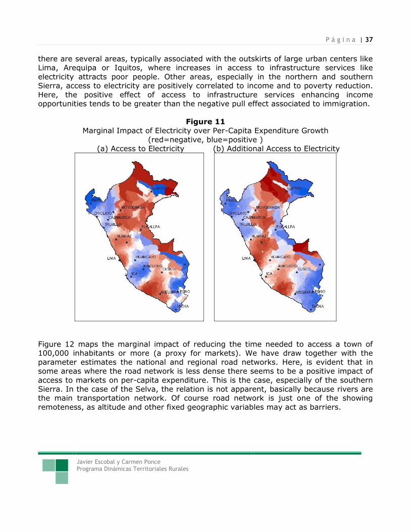
P á g i n a | 37


there are several areas, typically associated with the outskirts of large urban centers like Lima, Arequipa or Iquitos, where increases in access to infrastructure services like

electricity attracts poor people. Other areas, especially in the northern and southern Sierra, access to electricity are positively correlated to income and to poverty reduction.

Here, the positive effect of access to infrastructure services enhancing income opportunities tends to be greater than the negative pull effect associated to immigration.

Figure 11 Marginal Impact of Electricity over Per-Capita Expenditure Growth

(red=negative, blue=positive ) (a) Access to Electricity (b) Additional Access to Electricity

Figure 12 maps the marginal impact of reducing the time needed to access a town of 100,000 inhabitants or more (a proxy for markets). We have draw together with the

parameter estimates the national and regional road networks. Here, is evident that in some areas where the road network is less dense there seems to be a positive impact of

access to markets on per-capita expenditure. This is the case, especially of the southern Sierra. In the case of the Selva, the relation is not apparent, basically because rivers are the main transportation network. Of course road network is just one of the showing

remoteness, as altitude and other fixed geographic variables may act as barriers.

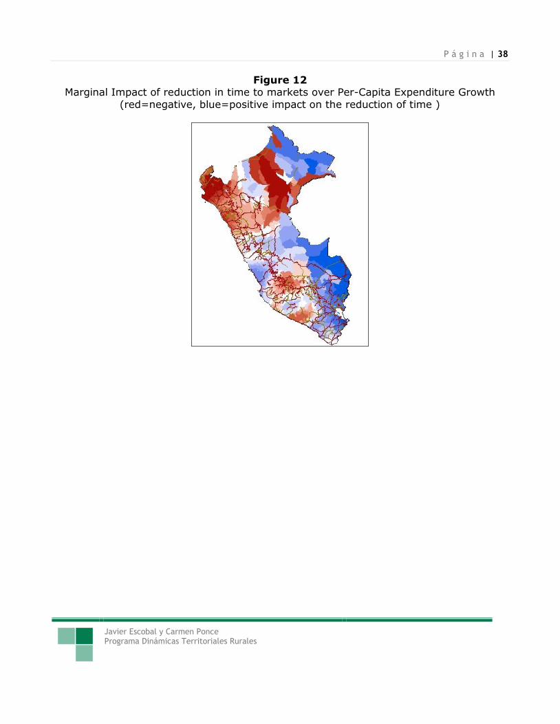
P á g i n a | 38


Figure 12 Marginal Impact of reduction in time to markets over Per-Capita Expenditure Growth

(red=negative, blue=positive impact on the reduction of time )

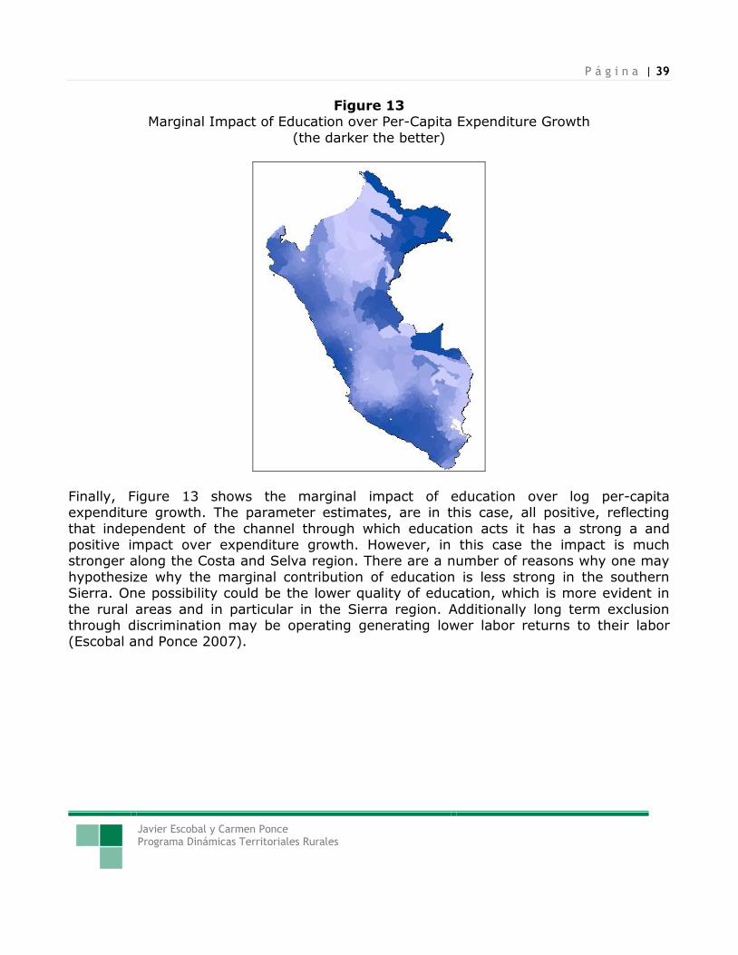
P á g i n a | 39


Figure 13 Marginal Impact of Education over Per-Capita Expenditure Growth

(the darker the better)

Finally, Figure 13 shows the marginal impact of education over log per-capita expenditure growth. The parameter estimates, are in this case, all positive, reflecting

that independent of the channel through which education acts it has a strong a and positive impact over expenditure growth. However, in this case the impact is much stronger along the Costa and Selva region. There are a number of reasons why one may

hypothesize why the marginal contribution of education is less strong in the southern Sierra. One possibility could be the lower quality of education, which is more evident in

the rural areas and in particular in the Sierra region. Additionally long term exclusion through discrimination may be operating generating lower labor returns to their labor (Escobal and Ponce 2007).

P á g i n a | 40


3. Final Remarks

This paper aims at evaluating up to what point spatial characteristics affect wellbeing

levels and changes of Peruvian household. Using poverty mapping exercises based on two contiguous censuses (1993 and 2005) we characterize the spatial distribution of poverty and poverty changes in an economy that grew on average 5% during this 12

year period. We find, indeed, that poverty and poverty changes are spatially correlated and we have also found that spatial characteristics - both first-nature and second-nature

geography” are correlated with this poverty indicators. Two effects that are particularly important are altitude and distance, a variable that proxies remoteness. This indicators show clearly that access to markets may be affected by remoteness, increasing the

likelihood of outward migration of the most educated and better endowed people and leaving behind the older, less educated and worst endowed people.

We found that there are a number of location specific variables (like access to infrastructure and market characteristics) as well as household specific variables that are

strongly correlated with wellbeing. It seems that pure geographic factors are associated with relative consumption per-capita, as well as access to infrastructure services, and

this correlation is reasonably robust even when we control for household, and location specific characteristics. However, the sign and the significance of this correlation do seem

to vary across space. This may be due to the fact that relative wellbeing does seem to have a persistent spatial correlation even after controlling for available geographic variables, infrastructure and household and context-specific characteristics.

Two possible explanations could be offered to explain why there is such a persistent

pattern of spatial correlation relative wellbeing even after controlling for geography and the above mentioned factors. One possibility is of course omitted variables and the second parameter heterogeneity. Omitted variables can be geographic or non-geographic

related. Since we have controlled for a large range of first-nature geographic variables (like altitude, temperature, precipitation, climate variability, and soil texture and quality)

we suspect that the bias is not geographic omitted variables. Another possibility is that other infrastructure services may have been omitted and these services themselves cannot be fully explained by the geographic variables already included in our profiles. Is

that is the case, since we have not been able to observe them we need just to correct for spatial correlation. Although we have done this, first order spatial correlation corrected

estimates continue to show significant spatially correlated errors. This persistent pattern of spatial correlation in the residuals forced us to focus our

attention in the possibility of parameter heterogeneity across space. Space can be geographic space but may also consider other dimensions like the welfare distribution

space. We have explored these two dimensions of spatial heterogeneity. The first one was modeled using quantile regressions while the second one has been explored using

P á g i n a | 41


geographically weighted regressions. Quantile estimation is based on the assumption of parameter variation across the wellbeing space. The results of both, however, highlight

the fact that welfare differences have persistence spatial characteristics, that cannot be fully accounted by observables characteristics including the most common geographic

variables, infrastructure, economic environment, private assets and, finally, human capital and household characteristics. Institutions are obviously a missing element that, although considered as an unobservable in this document, should be taken into account.

Recognizing the importance of the spatial dimension in such estimation procedures

stands out as a key factor to better understand poverty dynamics. This involves not only identifying spatial related covariates but also exploring further spatial correlation issues and potential parameter heterogeneity.

P á g i n a | 42


4. References

Brunsdon, C.; S. Fotheringham y M. Charlton (1998): “Geographically Weighted

Regression-Modelling Spatial Non-Stationarity”. The Statistician, 47(3) 431-443. Chesher, A. (1984): “Testing for Neglected Heterogeneity”. Econometrica 52(4), 865-

872.

Douidiche, M.; A. Ezzrari; and C. Ferré; and P. Lanjouw (2008): “Poverty Dynamics in Morocco’s Rural Communes: Tracking Change via Small Area Estimates”. Mimeo. World Bank. May 15, 2008

Dutta, J. and H. L. Leon (1991) “Testing for Heterogeneous Parameters in Least-Squares

Approximations”. The Review of Economic Studies, 58(2), 299-320 Elbers, C., J. Lanjouw, and P. Lanjouw (2004) Imputed welfare estimates in regression

analysis. Working Paper Series No. 3294. Washington, D.C.: World Bank.

Elbers, C., P. Lanjow and J. Lanjow (2000) Welfare in Villages and Towns: Micro-Level Estimation on Poverty and Inequality. World Bank

Escobal, J. and C. Ponce (2008) “Spatial disparities in living conditions in Peru: The role of geographic differences in returns vs. differences in mobile household assets

endowment, a cross section analysis”. Mimeo. World Bank-LAC. Lima June 2008.

Escobal, J. and C. Ponce (2007) “Economic Opportunities for Indigenous Peoples in Rural and Urban Peru.” In: Conference Edition: Economic Opportunities for Indigenous Peoples in Latin America . Washington DC.: World Bank.

Escobal, J.; M. Torero; and C. Ponce (2001) “Focalización Geográfica del Gasto Social:

Mapas de Pobreza” RED CIES de POBREZA GRADE-APOYO Informe Final Escobal, J. and M. Torero (2000): Does Geography Explain Differences in Economic

Growth in Peru? Inter-American Development Bank; Latin American Research Network. Research Network Working paper #R-404. Washington D.C.

Herrera, J. (2002): “La Pobreza en el Perú en 2001: Una visión departamental “. INEI-IRD. Lima – Perú, Mayo 2002.

Lanjouw, P., J. Lanjouw, C. Elbers and G. Demombynes (2007): “How good a map?

Putting small area estimation to the test”. Policy Research No 4155. Working Paper Series. The World Bank

P á g i n a | 43


Minier, J. (2007). "Institutions and parameter heterogeneity." Journal of

Macroeconomics, 29(3), 595-611.

Minot, N.; B. Baulch and M. Epprecht (2006): “Poverty and Inequality in Vietnam: Spatial Patterns and Geographic Determinants” (Research report 148. International Food Policy Research Institute. Washington D.C.

Nguyen , B.; J. Albrecht; S. Vroman; and M. Westbroo (2007): “A quantile regression

decomposition of urban–rural inequality in Vietnam”. In: Journal of Development Economics 83 (2007) 466–490.

Ravallion, M. and Woodon (1999) Poor areas or only poor people? Journal of Regional Science, Vol 39, No. 4, 1999, pp. 689-711

Vakis, R., J. Herrera and J. Escobal (2008) “Una mirada a la evolución reciente de la pobreza en el Perú: avances y desafíos”. Lima, Banco Mundial. 121 pp.

Zhao, Q and P. Lanjow (2005) Using Povmap2. Users guide. World Bank

Spatial patterns of growth and poverty changes in Peru ... · Spatial patterns of growth and...

Documents

Transcript of Spatial patterns of growth and poverty changes in Peru ... · Spatial patterns of growth and...