The Local Impact of Mining on Poverty and Inequality...
32
1 The Local Impact of Mining on Poverty and Inequality: Evidence from the Commodity Boom in Peru Norman Loayza Jamele Rigolini World Bank World Bank and IZA January 2016 Abstract This paper studies the impact of mining activity on socioeconomic outcomes in local communities in Peru. In the 1990s and 2000s, the value of Peruvian mining exports grew by fifteen times; and since early 2000s, one-half of fiscal revenues from mining have been devolved to local governments. Has this boom benefitted people in local communities? We present preliminary evidence to answer this question. Mining districts have larger consumption per capita and lower poverty rates than otherwise similar districts. However, these positive impacts decrease drastically with administrative and geographic distance from mining centers. Moreover, consumption inequality within mining districts is higher than in comparable nonproducing districts. This dual effect of mining is partially accounted for by the better educated immigrants required and attracted by mining activity. The inequalizing impact of mining, both across and within districts, may help explain the social discontent with mining in Peru, despite its enormous revenues. JEL: H7, I3, O1, Q3, R5 Keywords: Natural resources, Mining, Poverty, Inequality, Commodity Boom, Peru We are grateful to Alfredo Mier-y-Terán for collaborating with us on an earlier version of the paper and to Tomoko Wada, Juan Pablo Uribe, Phoebe Wong, Claudia Meza-Cuadra, and Jorge Franco for excellent research assistance. We have benefited from discussions and comments from Diether Beuermann, Laura Chioda, Ximena Del Carpio, Emanuela Galasso, Gianmarco León, Mónica Martínez-Bravo, Hugo Ñopo, Luis Servén, Renos Vakis, Cynthia van der Werf, and seminar participants at University Pompeu Fabra, CEMFI, University of Geneva, Universidad del Pacífico (Lima), GRADE (Lima), the Northeast Universities Development Consortium (NEUDC), the Latin America and Caribbean Economic Association (LACEA) Meetings (Sao Paulo), and the 2015 Annual Meetings of the Peruvian Economic Association (Lima). All remaining errors are our own. The findings, interpretations, and conclusions expressed in this paper are entirely those of the authors. They do not necessarily represent the views of the World Bank, its executive directors, or the governments they represent.
Transcript of The Local Impact of Mining on Poverty and Inequality...

1
The Local Impact of Mining on Poverty and Inequality:
Evidence from the Commodity Boom in Peru
Norman Loayza Jamele Rigolini
World Bank World Bank and IZA
January 2016
Abstract
This paper studies the impact of mining activity on socioeconomic outcomes in local communities in Peru. In the 1990s and 2000s, the value of Peruvian mining exports grew by fifteen times; and since early 2000s, one-half of fiscal revenues from mining have been devolved to local governments. Has this boom benefitted people in local communities? We present preliminary evidence to answer this question. Mining districts have larger consumption per capita and lower poverty rates than otherwise similar districts. However, these positive impacts decrease drastically with administrative and geographic distance from mining centers. Moreover, consumption inequality within mining districts is higher than in comparable nonproducing districts. This dual effect of mining is partially accounted for by the better educated immigrants required and attracted by mining activity. The inequalizing impact of mining, both across and within districts, may help explain the social discontent with mining in Peru, despite its enormous revenues.
JEL: H7, I3, O1, Q3, R5
Keywords: Natural resources, Mining, Poverty, Inequality, Commodity Boom, Peru
We are grateful to Alfredo Mier-y-Terán for collaborating with us on an earlier version of the paper and to Tomoko Wada, Juan Pablo Uribe, Phoebe Wong, Claudia Meza-Cuadra, and Jorge Franco for excellent research assistance. We have benefited from discussions and comments from Diether Beuermann, Laura Chioda, Ximena Del Carpio, Emanuela Galasso, Gianmarco León, Mónica Martínez-Bravo, Hugo Ñopo, Luis Servén, Renos Vakis, Cynthia van der Werf, and seminar participants at University Pompeu Fabra, CEMFI, University of Geneva, Universidad del Pacífico (Lima), GRADE (Lima), the Northeast Universities Development Consortium (NEUDC), the Latin America and Caribbean Economic Association (LACEA) Meetings (Sao Paulo), and the 2015 Annual Meetings of the Peruvian Economic Association (Lima). All remaining errors are our own. The findings, interpretations, and conclusions expressed in this paper are entirely those of the authors. They do not necessarily represent the views of the World Bank, its executive directors, or the governments they represent.

2
1. Introduction
To which extent do local communities benefit from extractive natural resources and commodity
booms? The question has been subject to wide but inconclusive research. This paper utilizes new data on
mining activity and government transfers in Peru to investigate the effect of mining and resource windfalls
on socioeconomic outcomes at the district level, the lowest administrative unit in the country.1
For two decades, Peru enjoyed an impressive mining boom. After decades of relative stagnation,
the value of mining exports doubled in the 1990s and then rose by more than seven times in the following
decade. By the early 2010s, the value of Peru´s mining exports averaged nearly 25 billion US dollars, or
14% of GDP and over 50% of total exports. At the beginning of the current decade, Peru was among the
five largest producers of silver, zinc, tin, lead, copper, gold, and mercury in the world. The mining boom
occurred while the country experienced high and sustained economic growth, which contributed to a
remarkable fall in poverty: between 2004 and 2007 alone, national poverty rates dropped by more than
15 percentage points, dropping by a further 20 percentage points – to 22.7 percent – by 2014.
Local Governments in producing regions have obtained large rents derived from mining activity.
The central Government transfers 50% of the taxes levied on mining companies to local governments in
mining regions. This sharing scheme, called the Mining Canon, has been implemented to decentralize
resource windfalls; it allocates funds to district, province, and regional governments according to a
distribution rule that favors producing localities. The sharing agreement was developed in the context of
a broader decentralization process that began in 2002.2 The Mining Canon’s distribution rule is dictated
and revised by national law.3 In 2007, the year of our analysis, the overall budget envelope of the Canon
amounted to approximately 1.6 billion US dollars.
1 In Peru, sub-national administrative units are called regions, provinces, and districts, where a region is composed of several provinces and, in turn, a province is composed of several districts. 2 To avoid the fiscal crises that had plagued earlier episodes of decentralization in Latin America, decentralization in Peru was heavily anchored around fiscal neutrality (World Bank, 2003). The ability of sub-national Governments to borrow was strictly limited by law, and the central Government imposed strong fiduciary requirements for spending (such as the need to submit proposals and receive clearance from the central Government for large capital investments). For districts, a law on participatory budgeting was also passed requiring local authorities, who are elected every four years, to consult each year with their constituency and civil society in planning the budget. 3 The Canon’s rule is as follows: 50 percent of mining tax revenues are distributed back to subnational governments. Of this amount, 10 percent goes directly to the corresponding producing district; 25 percent is distributed among all districts in a producing province; 40 percent is distributed among all districts in a producing region; and the remaining 25 percent is transferred to regional Governments and universities. Apart from the 10 percent transferred directly to producing districts, the allocation of the Canon across all (producing and non-producing districts) depends on district characteristics that include population size and socioeconomic conditions.

3
Yet, despite a substantial decline in poverty – both in urban and rural areas – and generous fiscal
transfers, the expansion of mining production has been accompanied by rising social tensions. In 2009,
the Office of the Ombudsman (Defensoría del Pueblo) reported 268 social conflicts in Peru, of which 38
percent were related to mining activities. Major confrontations involved violence and the use of firearms,
leading to death and injuries among protesters and the police (Taylor, 2011). These social tensions are a
major concern for policy makers, not least because they have halted or prevented large mining ventures:
It is estimated that by 2014 mining investment lost due to social conflicts amounted to $8-12 billion (4-
6% of GDP).4 While many protesters cite environmental concerns – and limited local participation in
environmental assessments may be an important factor behind conflicts (Jaskoski, 2014) – research
studies suggest that the underlying reasons are often more complex, involving revenue sharing disputes
between mining companies, local authorities, and local populations (Arellano-Yanguas, 2011, and Haslam
and Tanimoune, 2016).
In this paper we use variation in mining production across Peruvian districts to investigate the
impact of mining activity on local socioeconomic outcomes. The analysis uses a unique, district-level
dataset that merges administrative data (on local mining production and transfers from central to local
governments) with census and survey-based data (on average consumption, poverty, and inequality). The
main year of observation is 2007, when the latest national census took place.
Our identification strategy is based on comparing socioeconomic outcomes in mining producing
districts with outcomes in neighboring nonproducing districts of otherwise similar characteristics. Our
premise is that, while economic and political factors may influence international patterns of mining
activity, at lower administrative and geographic levels the location of mining production is primarily
dictated by geological factors. By comparing neighboring or nearby districts and controlling for initial
conditions, we can reduce biases related to endogenous location decisions.5
Figure 1 reports the location of mining districts and provinces across the Peruvian territory. It
shows that mining is concentrated in the Andean region and in the Amazon basin. To reduce potential
omitted variable biases, we restrict the analysis to regions that report mining activity, and we exclude the
province of Lima (where the influential and populous national capital is located). Our sample consists of
4 The figures on investment lost due to conflicts are based on Abusada (2014) and own calculations using information from the Ministry of Energy and Mining (MINEM). 5 As the recent opposition to the large Conga mine exemplifies, regional politics within a country can also affect the location of mining activity. That’s why we emphasize the within region and province variation when we discuss the results.
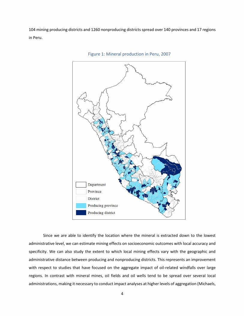
4
104 mining producing districts and 1260 nonproducing districts spread over 140 provinces and 17 regions
in Peru.
Figure 1: Mineral production in Peru, 2007
Since we are able to identify the location where the mineral is extracted down to the lowest
administrative level, we can estimate mining effects on socioeconomic outcomes with local accuracy and
specificity. We can also study the extent to which local mining effects vary with the geographic and
administrative distance between producing and nonproducing districts. This represents an improvement
with respect to studies that have focused on the aggregate impact of oil-related windfalls over large
regions. In contrast with mineral mines, oil fields and oil wells tend to be spread over several local
administrations, making it necessary to conduct impact analyses at higher levels of aggregation (Michaels,

5
2010). This runs the risks of missing some of the specific local effects and suffering from aggregation bias
(Caselli and Michaels, 2013).
Several preliminary findings emerge from our analysis. Mining activity appears to be beneficial for
districts where production takes place, resulting in higher consumption per capita and lower poverty and
extreme poverty rates than in comparable nonproducing districts. The benefits of mining activity,
however, seem to be unevenly distributed: Consumption inequality, as captured by the Gini coefficient,
is higher in districts of mining provinces and particularly in producing districts. Moreover, the benefits of
mining activity are localized to producing districts, with no discernable spillovers to other districts in the
same province, not even to close geographic neighbors. Therefore, mining appears to lead also to higher
inequality across districts.
After conducting a few robustness exercises, which confirm the basic results, we turn our
attention to assessing the impact of the Mining Canon itself and to understanding the mechanisms behind
the dual effect of mining activity. Regarding the Mining Canon, we use an instrumental variable procedure
to deal with its endogeneity and evaluate its impact.6 We construct an instrument based on a revenue
distribution rule that accounts for the district’s jurisdictional location and population but abstracts from
other socioeconomic characteristics. Once instrumented, the Canon does not seem to have a detrimental
effect on districts’ per capita consumption, poverty, or inequality.7 However, it does not appear to have a
beneficial effect either. This lack of impact is in line with some of the findings from studies focusing on oil
exploitation (Caselli and Michaels, 2013). It calls into question the impact of the current revenue sharing
design, in particular in the absence of strong monitoring and capacity building for subnational
governments (Bardhan and Mookherjee, 2006; Loayza, Rigolini and Calvo-Gonzalez, 2014).
In order to understand the mechanisms behind the positive (average) and negative
(distributional) effects of mining activity, we consider the differences between migrant and native
populations. Producing districts have a larger immigrant population than non-producing districts in the
same province or in other, non-producing, provinces. Producing districts have better educational
indicators than nonproducing districts, but alas, not because of differences across native populations but
because of their better-educated immigrants (arguably drawn by mining-related opportunities). On the
positive side, native populations in producing districts do have a larger share of salaried workers than
native populations in nonproducing districts. These results suggest that the better average outcomes
6 The Mining Canon distribution rule assigns larger allocations to poorer and less developed districts. 7 The OLS results show that a larger Mining Canon transfer is associated with lower consumption per capita and higher poverty index.
6
enjoyed by producing districts are, in part, explained by the better-educated (and presumably better-paid)
immigrants that mining activities require and attract and, only to some extent, explained by the jobs that
some natives (presumably the more qualified) are able to get. This may not only explain the better average
effects, but also the worse distributional outcomes regarding higher inequality.
Our findings add to a rich literature that investigates the impact of natural resource exploitation.
Early cross-country studies based on cross-sectional analyses (Sachs and Warner, 1995 and 2001) tend to
find a negative association between natural resource abundance and economic growth. However, studies
exploiting both cross-sectional and time-series variation find no effect or even a positive one (Manzano
and Rigobon, 2006; Raddatz, 2007). Differences in institutional settings and time horizons (short vs. longer
term) may explain in part these contrasting results (Mehlum, Moene and Torvik, 2006; Collier and Goderis,
2008; van der Ploeg, 2011; Boschini, Pettersson and Roine, 2013). Notwithstanding their contribution,
cross-country studies have suffered from uneven data quality and limited treatment of omitted variables
that may correlate with resource abundance.
More recent studies have attempted to solve some of these pitfalls by exploiting variation of
natural resource exploitation within national boundaries. These studies have mostly focused on oil
extraction. Michaels (2010) studies the impact of oil abundance in Southern U.S. counties on their long
term development. It finds that oil abundance increases local employment, population growth, per capita
income, and quality of infrastructure. 8 In developing countries with inferior institutional capacity,
however, the picture seems to reverse. Caselli and Michaels (2013) looks at the impact of backward
linkages and revenue windfalls from oil production across municipalities of similar characteristics in Brazil.
It finds no impact on GDP; and despite higher reported municipal spending on a range of budgetary items,
the paper finds little impact on social transfers, public good provision, infrastructure, and household
income. Moreover, Dube and Vargas (2006) finds that higher oil prices in Colombia boost conflict over the
ownership of resource production. Thanks to a greater ability to determine the location of mining activity
and the use of different socioeconomic outcomes, our analysis can measure local effects with more
precision and make progress in understand their mechanisms.
Our cross-district analysis also complements and builds upon existing studies of the local impacts
of mining on social and political outcomes. Sociological studies have found mining to play a fundamental
role in shaping rural development, as a product of the interaction between communities, mining
companies, and the State (Bebbington et al., 2008). An active literature has described a relationship
8 At a higher level of aggregation, however, Papyrakis and Gerlagh (2007) find a negative US state-level correlation between resource extraction and growth.

7
between mining exploitation and social conflict, rooted not only on environmental concerns but also on
competition for land resources, distribution of fiscal rents, and characteristics of the mining company and
concession site (Haslam and Tanimoune, 2016). A link between resource development and local inequality
in indigenous societies has also been postulated (O’Faircheallaigh, 1998), but existing research has
remained for the most part conceptual. A decentralized setting may add a layer of complexity. A study of
mining in the Philippines, for instance, finds that decentralized control over mineral resource wealth have
resulted in a highly ambiguous institutional arena, wherein heterogeneous actor coalitions attempt to
influence the associated distribution of mineral wealth (Verbrugge, 2015). This echoes the struggle
surrounding the management of the Mining Canon in the Peruvian context (Hinojosa, 2011).
Our findings complement and put in perspective existing econometric studies on mining in Peru.
Aragon and Rud (2013) study the effects of the Yanacocha gold mine in Peru, the second largest in the
world, and find a geographically widespread positive impact. The Yanacocha mine may, however,
represent a best-case scenario for two reasons: first, its sheer size may extend its impact beyond its
location; and, second, local living standards improved only after international shareholders put pressure
on Yanacocha’s management to expand local input procurement. Our findings are consistent with the
results of Zegarra, Orihuela and Paredes (2007) and Ticci and Escobal (2015), who, using a propensity
score matching methodology, look at the impacts of mining on poverty, migration, and labor-market
outcomes. Our econometric specification allows us to expand the analysis to spatial effects, to consider
the impact on inequality both within and across districts, and to isolate the effect of fiscal transfers (i.e.
the Mining Canon).
Finally, our analysis contributes, albeit tangentially, to an emerging literature on the political
economy of fiscal transfers and their use (Brollo et al., 2013). Studying local financing in Brazilian
municipalities, Litschig (2012) finds that local officials handle revenues derived from natural resources
differently than they do other transfers from the central Government: Only the latter seems to contribute
to human capital accumulation and poverty alleviation. These differences may stem from a greater ability
of local officials to capture commodity-related revenues, which is particularly pronounced when citizens
have little knowledge about their magnitude (Monteiro and Ferraz, 2010).
The paper is organized as follows. Section 2 presents the conceptual framework guiding our
empirical analysis, as well as the corresponding data and methodology. Section 3 shows and discusses the
results. Section 4 concludes.

8
2. Conceptual Framework, Data and Methodology
2.1 Conceptual Framework
There are several channels through which mining activity can affect socioeconomic outcomes.
Given the spatial and distributional focus of our analysis, in what follows we discuss the various channels
through these two lenses. These mechanisms can be divided into three broad categories. The first is direct
impacts and spillovers of mining on the local economy. Direct impacts on socioeconomic outcomes happen
to a large extent through the labor market, as a consequence of both direct hiring and increased local
economic activity.
By impacting local economic activity and offering better paid jobs, mining should have a positive
impact on local poverty rates. Nevertheless, the impacts on the native population remain a priori unclear.
Poverty rates can drop because mining offers better jobs to locals, but also because mining may attract
better paid immigrants, so that in relative terms there are fewer poor people. Likewise, the impacts on
inequality remain a priori ambiguous: depending on whether mining activity benefits skilled more than
unskilled workers or attracts a more skilled mix of workers, inequality could increase. It is therefore
possible to observe mining both reducing poverty and increasing inequality.
The second channel through which mining may affect local socioeconomic outcomes is financial
transfers to local municipalities, provinces, and regions stemming from mining revenues (i.e. the Mining
Canon). Such transfers can have an ambiguous impact on both poverty and inequality. First, there is
evidence that many municipalities have trouble just managing to spend these additional revenues (Loayza,
Rigolini, and Calvo-Gonzalez, 2014). Second, depending on the type of investments, the Mining Canon
may have a distributional impact that favors the better-off. Third, some of these rents may be
misappropriated through corruption of politicians and people in power.
The third channel are direct investments of mining companies in producing districts. Mines,
especially large ones, often invest in infrastructure improvements, such as the quality of the road network,
that benefit both their own activities and the population at large. It is also the case that large mines
contribute directly to local development projects (see Ticci and Escobal, 2015). On average, these direct
investments should have a positive effect on poverty – albeit confined to districts close to the mining
center – while, here as well, the impact on inequality will depend on the type of investments.
The conceptual framework predicts that mining should have a positive impact on poverty.
However, the impact of inequality is a priori ambiguous. It would depend on whether mining induces
immigration of skilled workers and better employment opportunities for local workers, whether the
Mining Canon is used to benefit particular groups of the population, whether the public and private
9
investment projects have a distributional impact, and whether these labor and capital effects are
geographically limited or widely dispersed. Given this conceptual motivation, we begin the empirical
analysis by looking at the overall impacts of mining on poverty and inequality depending on administrative
and geographic proximity; we then consider the impact of the Mining Canon. To conclude, we examine
whether native and immigrant populations are different regarding education and employment, in order
to suggest the mechanisms underlying our results.
2.2 Data
The unit of observation and analysis is the district, which is the smallest administrative unit in the
country. In Peru, a group of districts forms a province, and a group of provinces forms a region. The
boundaries between them are based on historical and political jurisdictions and revised only rarely.9 The
advantage of using district-level analysis is that it allows the most precise identification of local effects
resulting from mining activity. We only work with districts belonging to regions where some mining
production took place in the five years prior to the year of observation, 2007, and we exclude districts in
the province of Lima, where the country’s capital is located (which makes the province an outlier in most
respects). The resulting sample consists of 1364 districts in 140 provinces and 17 regions. Appendix Table
A1 provides information on definitions and sources of all variables used in the paper, and Appendix Table
A2 presents some summary statistics across groups of districts.
As dependent variables, we consider a set of socioeconomic outcome indicators (at the district
level). For purposes of this paper, the most important of them are derived from the country’s “poverty
map” for 2007: average per capita consumption, poverty and extreme poverty headcount indexes, and
the Gini coefficient of consumption inequality. The poverty map was developed by the Peruvian Statistical
Institute, combining data from the 2007 Census and the 2007 National Household Survey (INEI, 2009) and
following a methodology based on Hentschel, Lanjouw, Lanjouw, and Poggi (2000). In some applications,
we also use indicators directly obtained from the National Censuses of 2007 and 1993: illiteracy rate,
average years of education of the adult population, immigration rate, employment rate, and public and
private infrastructure measures.
Admittedly, by using 2007 as our measurement year, we miss the part of the mining bonanza that
happened subsequently. Nevertheless, between 1993 and 2007, an impressive mining boom that
multiplied the value of mining exports by about 10 times had already occurred (and just during the
preceding five years, 2002-07, mining exports increased by a factor of 5). At any rate, 2007 is the date of
9 Peru is divided into 25 regions, 195 provinces, and 1841 districts.

10
the last Census and poverty map, and it is the last period for which reliable district-level poverty and
inequality information can be obtained.
We use two sets of explanatory variables. The first and most important are indicators of the
location and magnitude of mining activity, as well as measures of fiscal revenues accruing to districts
according to the Mining Canon Law; the second one is a set of control variables chosen to account for
initial differences across districts. Using plant-level mining data from the Peruvian Ministry of Energy and
Mining (MINEM), we distinguish three types of districts within mining regions: Producing districts, which
host a mining facility with some mineral production during 2002-2006 and receive the largest share of the
Canon; non-producing districts in producing provinces, which, despite not having a mining facility, receive
a portion of the Canon and could be under the economic influence of mining districts; and non-producing
districts in non-producing provinces, which receive the lowest share of the Canon and are the least
affected by mining activity in the sample. Our sample contains 104 producing districts, 563 non-producing
districts in producing provinces, and 697 non-producing districts in non-producing provinces.
Apart from these categorical variables (that is, dummy variables corresponding to the three types
of districts), we also use information on the magnitude of mining production and related fiscal revenues.
The magnitude of mining activity at the district level is measured as the accumulated value of mineral
production by all mining facilities within the district for the period 2002-2006. We obtain the value of
mineral production by combining data on production quantities by type of mineral with international
prices per mineral, both reported by the Ministry of Energy and Mining (MINEM).10 Similarly, Mining
Canon revenue at the district level is the accumulated value of fiscal transfers received by each district
during 2002-2006, as reported by the Ministry of Economy and Finance (MEF).
The second set of explanatory variables consists of control variables, which account for
differences across districts other than mining activity or its revenues. First, we include time-invariant
district characteristics, such as surface area, altitude, and a binary variable indicating whether the district
is a provincial capital. Second, we include district-specific initial conditions, taken from the 1993 Census,
such as total population, percentage of rural population, percentage of households with access to clean
water and sanitation, percentage of households with electricity, the illiteracy rate, and the percentage of
the working-age population with paid work. In addition, to control for remaining characteristics as
perceived by the central government, we include the transfers from the central to district governments
10 MINEM’s production data are disaggregated by type of mineral. We consider the eight minerals whose production accounts for nearly 100% of mining production in the country. They are, gold, silver, copper, zinc, lead, tin, iron and molybdenum.
11
to fund public services and goods. These transfers, grouped under the program Foncomun, are separate
from the mining-related transfers of the Canon. Our measure consists of the accumulated Foncomun
transfers received by each district during 2002-2006, as reported by the Ministry of Economy and Finance.
2.3 Methodology
Our identification strategy relies upon comparing localities that are spatially close and
institutionally similar but differ regarding mining activity. In order to work with similar localities, we use
the administrative demarcation of localities into districts, provinces, and regions, focusing on the
comparisons between districts belonging to the same region or province. We conduct these comparisons
by means of several exercises, which are explained in detail in the following section. Using terms from
experimental design, we can consider having two treatment groups --producing districts and
nonproducing districts in producing provinces-- and a control group --districts in nonproducing provinces.
The comparisons of interest are between each of the treatment groups with the control group, and
between the treatment groups with each other.
The basic, benchmark regression equation is the following,
𝑌𝑑 = 𝛽0 + 𝛽1𝕀𝑑[𝑃𝐷] + 𝛽2𝕀𝑑[𝑁𝑃𝐷𝑃𝑃]+ 𝛽3𝐷𝑑 + 𝛽4𝑋𝑑 + 𝜈𝑅 + 𝜈𝑝 + 𝜀𝑑 (1)
Where, 𝑑 denotes district, 𝑌𝑑 represents a given outcome variable, 𝕀𝑑[𝑃𝐷] is a binary variable that takes
the value of 1 if the district is producing and 0 otherwise, 𝕀𝑑[𝑁𝑃𝐷𝑃𝑃] is a binary variable that takes the
value of 1 if the district is non-producing in a producing province and 0 otherwise, 𝑋𝑑 is a set of initial
conditions, 𝐷𝑑 is a set of time-invariant district characteristics, 𝜈𝑅 is a region fixed effect, 𝜈𝑝 is a province
fixed effect, and 𝜀𝑑 is an error term.
Note that the interpretation of the coefficients of interest, 𝛽1and 𝛽2, depends on whether region
and/or province fixed effects are included. When neither region nor province fixed effects are included,
𝛽1 estimates the difference in means between producing districts (treatment 1) and districts in
nonproducing provinces (control) in any region; and 𝛽2 estimates the difference in means between
nonproducing districts in producing provinces (treatment 2) and districts in nonproducing provinces
(control) in any region. In the tables presented in the paper, these estimates are given under the heading
“Across and Within Regions.” When region fixed effects are included but not province fixed effects, the
meaning of 𝛽1and 𝛽2 is similar as above but the comparison is restricted to districts within the same
region. In the tables, these estimates are presented under the heading “Within Region.” Finally, when
province fixed effects are included, 𝕀𝑑[𝑁𝑃𝐷𝑃𝑃] drops out, and 𝛽1 estimates the difference in means
between producing districts (treatment 1) and nonproducing districts in the same province (treatment

12
2).11 These estimates are presented under the heading “Within Province.”
The quality of the identification strategy depends on whether treatment and control districts were
similar before the “treatment” started, that is, before the mining boom. As mentioned previously, mining
activity picked up in Peru in the 1990s and 2000s, with the international commodity boom and the
propitious macroeconomic and business conditions in the country. However, mining has been historically
important for Peru, and there has always been some mining in certain areas of the country. There are,
therefore, reasons to believe that producing and nonproducing districts were not initially similar.
Ideally, we would have liked to have a baseline with information on the outcome variables of
interest (income, poverty, and inequality) at an initial period. Then, we could have conducted a difference-
in-difference type of comparison. Unfortunately, however, a poverty map before the mining boom is
unavailable and cannot be constructed: The previous census, conducted in 1993, was not accompanied
by a household survey that would provide income or consumption information.
Nevertheless, we are able to check for some initial differences across districts, prior to the mining
boom, using information from the 1993 Census. We consider district-level initial conditions regarding
population, education, work, and infrastructure. We conduct the comparison across treatment and
control groups by applying the following regression:
𝑋𝑑 = 𝛼0 + 𝛼1𝕀𝑑[𝑃𝐷] + 𝛼2𝕀𝑑[𝑁𝑃𝐷𝑃𝑃]+ 𝛼3𝐷𝑑 + 𝜈𝑅 + 𝜈𝑝 + 𝜇𝑑 (2)
Where, 𝑋𝑑 represents a given initial condition, and all other variables are as in equation (1).
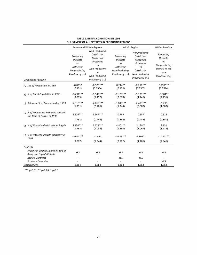
The results in Table 1 indicate that as of 1993 there were differences between producing and
nonproducing districts and, in general, between treatment and control groups. Moreover, with the
exception of the proportion of households with electricity, these differences were rather in favor of
districts in producing provinces, especially those where mining took place. These differences are reduced
when we compare districts within the same region and province but do not fully disappear. The results
highlight the importance of controlling for region and province effects and suggest the need to include
controls for initial and time-invariant district characteristics, specifically those listed above.
3. Results
Using the sample and data outlined above, we conduct the following empirical exercises. First,
we present the basic results of comparing the treatment and control groups. Second, we conduct some
variations of the basic specification to check for the robustness of the results. Third, we study to what
11 Naturally, when province fixed effects are included, region fixed effects become redundant.

13
extent the effects of mining activity are localized geographically, in the sense of applying only to producing
districts without spillovers to their neighbors. Fourth, we consider whether the Mining Canon has an effect
on its own and whether it affects the basic results of mining activity. And fifth, we examine a likely
mechanism by contrasting outcomes from the overall district population with outcomes from its native
population.
3.1 Basic results
Our basic, benchmark results are obtained from estimating regression equation (1), presented
above. That is, we estimate the difference in means between treatment and control groups for four
outcome variables at the district level: Average per capita consumption, the poverty headcount index, the
extreme poverty headcount index, and the Gini coefficient of consumption inequality across households.
As mentioned in the previous section, these variables are obtained from the Peru Poverty Map
corresponding to 2007. The results are presented in Table 2.
Producing districts (treatment 1) have larger consumption per capita and lower poverty and
extreme poverty indexes than non-producing districts, whether the latter are in the same province
(treatment 2) or in a non-producing province (control). At the same time, however, producing districts
have larger income inequality than non-producing districts. The differences between non-producing
districts in a producing province and non-producing districts elsewhere in the same region are not
significant, except for income inequality. Therefore, mining activity appears to be related to increased
inequality both within producing districts and across districts in the same or other provinces.
The differences in means tend to be larger in size and more statistically significant when
comparisons are not limited to the same region or province (first two columns, labeled “Across and Within
Regions”). The quality of the identification strategy improves when comparisons are restricted to districts
in the same region (intermediate columns, labeled “Within Region”). Although the size and significance of
the effects decline, they are arguably more reliable. The sharpest comparison is between the two
treatment groups, when we restrict the comparisons to districts within the same province (last column,
labeled “Within Province”). Focusing on the last set of results, producing districts have about 9 percent
larger per capita consumption than nonproducing districts and 2.6 percentage points less poor and
extreme poor population. On the negative side, the Gini coefficient of (consumption) inequality is 0.6
percentage points larger in producing than nonproducing districts.
3.2 Robustness
To check the robustness of the results, we extend the analysis along three dimensions. First, we
use propensity score matching to select comparable districts among our sample, as an alternative to

14
controlling for initial conditions via multiple regression analysis. Second, we take into account the
magnitude of mineral production, as an alternative to using a binary, dummy variable approach to
characterizing districts in producing provinces. Third, we consider different samples and additional control
variables.
Propensity score matching
As an alternative to using control variables in a regression setting, we use a matching procedure
to select comparable producing and nonproducing districts. Specifically, we match producing districts with
various subsamples of non-producing districts of similar characteristics using a propensity score built upon
a probit regression. With the exception of accumulated Foncomun transfers, the matching variables are
the same time-invariant characteristics and initial (1993) conditions used as controls in the basic
regression12. In addition, to obtain the “Within Region” results, we restrict matches to districts in the same
region and then perform the match based on the propensity scores; and we follow an analogous
procedure to obtain the “Within Province” results. (Obviously, for the “Across and Within Regions” results,
we exclude region and province restrictions and match districts solely on their propensity scores.) We
then estimate the Average effect of Treatment on the Treated (ATT) using an Epanechnikov Kernel with a
bandwidth of 0.2. We obtain standard errors through bootstrapping, using 100 repetitions. The results
are presented in Table 3.
The propensity score matching approach is supportive of the basic regression results. Producing
districts have higher average per capita consumption and lower poverty and extreme poverty headcount
indexes than non-producing districts. These results are uniformly statistically significant when comparing
districts across and within regions (first column) and within the same province (last column). The results
carry the same signs but are not statistically significant when restricting the comparison to the same
region (third column). Also as in the benchmark case, producing districts suffer from higher inequality
than any other group of districts, and this result is always statistically significant. Non-producing districts
in producing provinces also suffer from higher inequality than districts in nonproducing provinces that are
in the same region (fourth column). Focusing on the within province results, the mean differences
between producing and nonproducing districts in the same province are larger in magnitude than those
obtained under the basic regression.
Magnitude of production
12 As described in Caliendo and Kopeinig (2005), covariates should only be included in the propensity score model if they are either fixed over time or measured before participation in the treatment (i.e. being a producing district). For this reason, Log of Accumulated Foncomun Transfers Per Capita in Soles for 2002-2006 is not included.

15
Producing districts do vary regarding the value of their mining production. The basic specification
does not take into account this variation, and we now check whether accounting for the value of
production affects the main results. For this purpose, regression equation (1) is transformed into the
following,
𝑌𝑑 = 𝛽0 + 𝛽1𝕀𝑑[𝑃𝐷] ∗ 𝑃𝑟𝑜𝑑𝑑 + 𝛽2𝕀𝑑[𝑁𝑃𝐷𝑃𝑃] ∗ 𝑃𝑟𝑜𝑑𝑝 + 𝛽3𝐷𝑑 + 𝛽4𝑋𝑑 + 𝜈𝑅 + 𝜈𝑝 + 𝜀𝑑 (3)
Where, 𝑃𝑟𝑜𝑑𝑑 is the (log of 1 plus the) accumulated value of mineral production per capita in the district
between 2002 and 2006, and 𝑃𝑟𝑜𝑑𝑝 is the (log of 1 plus the) accumulated value of mineral production
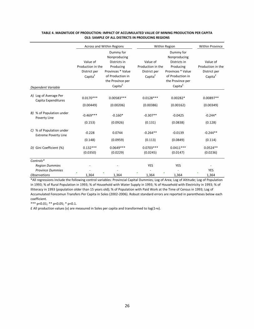
per capita in the corresponding province over the same period.13 The results are presented in Table 4.
The estimation results that take into account the value of mining production confirm those of the
basic specification in all relevant respects. The interpretation of the coefficients, however, is somewhat
different since in this case the magnitude of mining activity matters. Larger values of mineral production
in a district are related to higher average per capita consumption, lower poverty and extreme poverty
indexes, and higher inequality. The coefficient sizes tend to get smaller as region and then province fixed
effects are included, remaining however statistically significant. (As in the basic results, the exception is
the regression for the index of extreme poverty: there, the coefficient on the value of production becomes
larger and statistically significant when comparing across districts in the same region or in the same
province.) For non-producing districts, the value of production in their province seems to be related to
higher average per capita consumption and higher inequality, with no clear effect regarding poverty rates.
Other Robustness Checks
We conduct three other robustness checks. The first one expands the set of producing districts by
including, in addition, those whose jurisdiction had been divided into two or more districts after 1993 and
those that have been identified as mining districts by both Ticci and Escobal (2015) and Zegarra, Orihuela,
and Paredes (2007). The number of producing districts then increases from 104 to 116. The second
robustness check restricts the sample of districts to those located in the highlands of the country (Sierra).
This region includes the most traditional mining areas in the country and arguably comprises a more
homogenous sample (than in the benchmark regression). The third robustness check adds two additional
control variables: An “index of unsatisfied basic needs” generated by the Peruvian Government and based
on household characteristics regarding living conditions, access to public infrastructure, education, and
earning capacity, using information from the 1993 Census. From the same source, we also add the
13 The indicator variable 𝕀𝑑[𝑃𝐷]in equation (3) is redundant. We include it for clarity purposes.

16
percentage of households in the district that are headed by a female. This attempts to take into account
the impact of the 1980s civil conflict that affected a considerable portion of Peruvian districts, particularly
in the highlands. The results of the three robustness checks are presented is respective panels of Table 5.
The results using the extended set of producing districts are similar to those of the benchmark
regression. The estimated coefficients when using the extended sample have the same sign but are slightly
smaller and no longer significant in the case of extreme poverty. These changes are to be expected given
the imprecision introduced by relaxing the selection of “treatment” districts. In contrast, when the sample
is restricted to districts in the highlands, the coefficients not only maintain their sign but are also larger
than in the benchmark specification, in absolute terms and relative to their respective standard errors.
This implies strengthening the statistical significance of the estimated effects. This is particularly true for
poverty and extreme poverty. Finally, when the additional controls on unsatisfied basic needs and female-
headed households are added, the results are almost the same as in the benchmark regression, regarding
sign, size, and significance of the coefficients, especially when region- and province-specific effects are
taken into account.
All in all, we can conclude that, with specific nuances, the basic results are quite robust: mining
districts have larger average consumption, lower poverty rates, and higher inequality than non-mining
districts, whether in the same province or not; likewise, non-mining districts in producing provinces are
similar in all respects to other non-mining districts, except that those in mining provinces have higher
inequality.
3.3 Localized effects
We now study to what extent the effects of mining activity are localized; that is, whether they
apply only to producing districts without spillovers to their geographic neighbors. For this purpose, in
addition to using administrative jurisdictions to identify treatment and control groups, we employ a
criterion based on geographic proximity. Specifically, we use mapping software to identify first-order and
second and higher-order neighbors of mining districts. First neighbors share a border with producing
districts, second neighbors share a border with first neighbors, and so on. (Producing districts are
identified as such, and not as neighbors of other producing districts.) For this extension, regression
equation (1) is transformed into the following,
𝑌𝑑 = 𝛽0 + 𝛽1𝕀𝑑[𝑃𝐷] + 𝛽2𝕀𝑑[𝐹𝑖𝑟𝑠𝑡 𝑁𝑒𝑖𝑔ℎ𝑏𝑜𝑟]+ 𝛽3𝐷𝑑 + 𝛽4𝑋𝑑 + 𝜈𝑅 + 𝜈𝑝 + 𝜀𝑑 (4)
Under this specification, first neighbors belong to treatment 2, and second and higher-order
neighbors correspond to the control group. Note that in this case, 𝕀𝑑[𝐹𝑖𝑟𝑠𝑡 𝑁𝑒𝑖𝑔ℎ𝑏𝑜𝑟] is not dropped

17
when province dummies are included, and, therefore, 𝛽1and 𝛽2 can both be estimated within provinces.
This approach can be useful in two aspects. First, by focusing attention on districts that share borders and
are more likely to be similar, this exercise may help address further potential omitted variable biases.
Second, it allows exploration of how much geographic proximity, beyond purely administrative
jurisdiction, matters for identifying the effects of mining activity. In particular, while under the basic
specification all non-producing districts in producing provinces are treated as equals, the specification in
equation (4) allows us to distinguish between first and higher-order neighbors within the same province.
The results are presented in Table 6, focusing only on the within-province comparisons.
The comparisons based on geographic proximity confirm the results of the basic specification,
with support for the notion of localized effects. Producing districts have larger average per capita
consumption and lower poverty rates than neighboring districts. On the other hand, producing districts
also present larger inequality than neighboring districts. Regarding the positive effects (i.e., larger average
consumption and lower poverty rates), producing districts are almost as different from first neighbors as
they are from second (and higher-order) neighbors: the sizes of the coefficients measuring the mean
difference between producing districts and the rest are around the same as in the basic regression. For
consumption and poverty rates, the estimated differences between first and second (and higher-order)
neighbors are not statistically significant. Regarding the negative effects (i.e., larger Gini coefficient),
producing districts have more inequality than first neighbors, and they, in turn, feature larger inequality
than second (and higher-order) neighbors. These results suggest that the positive effects of mining are
confined to producing districts.
3.4 The Canon
We now turn to analyzing the Mining Canon, with the dual purpose of evaluating its effect on
poverty and inequality and checking whether including it affects the basic results of mining activity. For
this purpose, regression equation (3) is augmented as follows,
𝑌𝑑 = 𝛽0 + 𝛽1𝑃𝑟𝑜𝑑𝑑 + 𝛽2𝕀𝑑[𝑁𝑃𝐷𝑃𝑃] ∗ 𝑃𝑟𝑜𝑑𝑝 + 𝛽3𝐷𝑑 + 𝛽4𝑋𝑑 + 𝛽5 ∗ 𝐶𝑎𝑛𝑜𝑛𝑑 + 𝜈𝑅 + 𝜈𝑝 + 𝜀𝑑 (5)
Where, 𝐶𝑎𝑛𝑜𝑛𝑑 is the (log of 1 plus) the accumulated value of government transfers during 2002-2006,
made in accordance to the Mining Canon Law of 2002 and its addendums. Arguably, regression equation
(5) should not be estimated directly by OLS because Canon transfers are jointly endogenous with the
dependent variables. In fact, the Mining Canon’s distribution rule (for district, province and region
allocations) factors in socioeconomic indicators that are closely connected with income, poverty, and
inequality measures.

18
We use an instrumental variable (IV) procedure to deal with the endogeneity of the Canon. We
construct an instrument based on a revenue distribution rule that takes into account the district’s
jurisdictional location and population, while abstracting from other socioeconomic characteristics. Thus,
the instrument considers the revenue shares mandated by law according to the location of production
(district, province, and region) and population weights. Since 2002, there have been 3 revenue
distribution regimes (corresponding to the original canon law and its 2 subsequent modifications). They
respectively apply to: 2002-03, 2004, and 2005-present. The instrument is built by following the specific
rules of the corresponding regime per year and then accumulating for the period 2002-06. This is done
both in total and per capita terms, resulting in 2 instruments. Since only overall revenues at the regional
level could be obtained directly from the data, we use the assumption that province and district revenues
are proportional to their respective value of mining production. Table 7 presents the results obtained
with instrumental variables (through a GMM estimator), and the OLS results for comparison purposes.
We focus on the within-province exercise.
Taken at face value, the OLS results suggest a significant association between larger Canon
transfers and worse socioeconomic conditions: lower average per capita consumption and higher poverty
headcount index. This likely reflects the fact that the Canon allocation is larger for districts that are more
in need. In fact, the IV results confirm that the negative OLS results are due to reverse causation: Once
instrumented, the Canon does not seem to have a (statistically significant) detrimental effect on districts’
per capita consumption and poverty rate. However, it does not appear to have a beneficial impact either.
This is an interesting and important topic and deserves further research study.
Finally, the coefficients on the value of mining production retain their sign and significance after
the Canon transfer is included. This, together with the lack of a significant Canon effect, suggests that the
socioeconomic impact of mining is related to the economic activity itself, rather than the fiscal revenues
it generates.
3.5 The mechanism: migrants or natives?
Our analysis uses the district as the unit of observation. This is not only due to data limitations but
also to our concern for understanding outcomes at the community level. Districts are not, however,
homogenous entities, and aggregate local effects may mask differing impacts on the population. Of
particular interest to understand the mechanism of mining effects is the difference between migrant and
native populations. The poverty map does not have information at the household level, so that studying
the disaggregated effects on consumption and poverty by groups within a district is not feasible. Census
data can, however, shed light on our results.

19
The 2007 Census allows distinguishing between native and immigrant populations. It reports
whether the mother of a respondent living in a district was a resident of the same district when the
respondent was born. If this is the case, we identify the person as native, and otherwise as immigrant.14
Then, the first question to address is whether there are significant differences across districts regarding
immigration. The results are reported at the bottom of Table 2. Producing districts have larger immigrant
populations than non-producing districts in the same province or in other, non-producing, provinces. In
fact, the share of immigrants in the total population is over 6 percentage points higher in producing than
nonproducing districts.
This raises the question as to whether the better consumption and poverty outcomes observed
for mining districts are due to their having wealthier and more educated immigrants. To address this
question we compare educational and labor indicators for total and native populations. We present only
the mean differences between producing and nonproducing districts in the same province (for which
identification is arguably the most precise).15 The results, presented in Table 8, are remarkable. The
educational differences observed for the whole population are driven by immigrants’ characteristics:
Producing districts have better educational indicators than nonproducing districts because of their well-
educated immigrants, not because of differences across native populations. On the positive side, native
populations in producing districts do have a larger share of salaried workers than native populations in
nonproducing districts.
These results suggest that the better average outcomes enjoyed by producing districts are in part
explained by the well-educated (and presumably well-paid) immigrants that mining activities require and
attract. To some extent, this may explain not only the better outcomes regarding consumption per capita
and poverty headcount index but also the worse outcomes regarding inequality. We should not, however,
ignore the positive impact of mining on the salaried employment of natives: some of them, presumably
the more qualified, seem to get jobs in mining and related economic activities.
4. Conclusions
Mining has a dual impact on local communities in Peru: It has a positive average effect but a
negative distributional effect. On the positive side, producing districts have 9 percent larger per capita
consumption than comparable nonproducing districts and 2.6 percentage points less poor and extreme
14 The results are robust to other criteria for identifying native population; for instance, whether the head of household has lived in the district for more than five years. 15 The results are similar for comparisons between producing districts and districts in nonproducing provinces (treatment 1 vs. control).

20
poor population. On the negative side, the Gini coefficient of inequality is 0.6 percentage points larger in
producing than nonproducing districts. Moreover, the positive average benefits are limited to producing
districts, with no discernable spillovers to other districts even in the same province. Mining, therefore,
appears to lead to higher inequality both within and across local communities.
Mining’s dual effect is partly explained by the well-educated (and surely well-paid) immigrants
that mining activities require and attract to producing localities. It is also explained by the jobs that some
community natives (likely the more qualified) are able to get in industries and services related to mining
activity. The distributional impact of mining may explain, at least in part, the social discontent regarding
mining activities in the country.
The paper highlights some areas for future research. The first has to do with a better
understanding of the connection between social conflict and natural resource extraction. We have
underscored the importance of economic distributional effects. Other literature has also highlighted the
capture of rents by local politicians, concerns about environmental damage, and cultural alienation of
native populations, to name a few. Understanding how these factors influence on their own and interact
with each other may elucidate communities’ perceptions on the benefits and damages stemming from
mining activity, as well as the changes needed for mining to be accepted by local populations.
The second area for future research is regarding the usefulness of fiscal transfers to local
governments. In principle these transfers can fund public goods and services that increase welfare in local
communities and counteract any possible negative impacts derived from mining activity. We find neither
a detrimental nor a beneficial effect from the Mining Canon in Peru. One possibility is that by 2007 it was
too soon to obtain any significant effects from a decentralization program that had been working for 5
years. Another possibility is that decentralization in Peru is rather flawed and must be restructured,
decreasing the incentives for capture of local governments and improving their managerial and
implementation capacity.
Solving the social discontent with mining and allowing mining to reach its full potential on local
communities will require a broader discussion and overarching institutional reforms encompassing fiscal,
governance, and productive aspects. Should people in local communities be made co-owners of mining
companies, by distributing among them stockholder rights and dividends? Should the management of
mining revenues be only one component, albeit important, in a comprehensive reform of fiscal
decentralization in Peru and other countries facing similar issues?

21
References
Abusada, R. (2014). “Perspectivas y viabilidad de la actividad minera en el Perú.” Presentation made at the 11th International Symposium on Gold and Silver. http://www.simposium-del-oro.snmpe.pe/11-simposium-del-oro-ponencias.html#
Aragon, F. M. and Rud, J. P. (2013). “Natural Resources and Local Communities: Evidence from a Peruvian Gold Mine.” American Economic Journal: Economic Policy. 5(2): 1-25.
Arellano-Yanguas, J. (2011). “Aggravating the Resource Curse: Decentralisation, Mining and Conflict in Peru.” Journal of Development Studies. 47(4): 617-38.
Bardhan P., and Mookherjee, D. (2006). Decentralization and Local Governance in Developing Countries. The MIT Press. Cambridge, MA.
Bebbington, A., Humphreys Bebbington, D., Bury, J., Lingan, J., Muñoz, J.P. and Scurrah, M. (2008), “Mining and Social Movements: Struggles Over Livelihood and Rural Territorial Development in the Andes,” World Development, 36(12): 2888-2905.
Boschini, A., Pettersson, J. and Roine, J. (2013), “The Resource Curse and its Potential Reversal,” World Development, 43: 19-41.
Brollo, F., Nannicini, T., Perotti, R. and Tabellini, G. (2013). “The Political Resource Curse.” American Economic Review. 103(5): 1759-96.
Caliendo, M. and Kopeinig, S. (2005). “Some Practical Guidance for the Implementation of Propensity Score Matching.” IZA Discussion Papers, 1588.
Caselli, F. and Michaels, G. (2013). “Do Oil Windfalls Improve Living Standards? Evidence from Brazil.” American Economic Journal: Applied Economics. 5(1): 208-38.
Collier, P. and Goderis, B. (2008). “Commodity Prices, Growth, and the Natural Resource Curse: Reconciling a Conundrum.” OxCarre Research Paper. 2008-14.
Dube, O. and Vargas, J. F. (2006). “Commodity Price Shocks and Civil Conflict: Evidence from Colombia.” Review of Economic Studies. 80 (4): 1384-1421.
Hentschel, J., Lanjouw, J. O., Lanjouw, P. and Poggi, J. (2000). “Combining Census and Survey Data to Trace the Spatial Dimensions of Poverty: A Case Study of Ecuador.” The World Bank Economic Review. 14 (1): 147-165.
Hinojosa, L. (2011). “Riqueza Mineral y Pobreza en Los Andes.” European Journal of Development Research. 23(3): 488-504.
Instituto Nacional de Estadística e Informática (2009). Mapa de Pobreza Provincial y Distrital 2007: El Enfoque de la Pobreza Monetaria. http://www.inei.gob.pe
Jaskoski, M. (2014), “Environmental Licensing and Conflict in Peru’s Mining Sector: A Path-Dependent Analysis,” World Development, 64: 873-883.
Litschig, S. and Morrison, K. M. (2013). “The Impact of Intergovernmental Transfers on Education Outcomes and Poverty Reduction.” American Economic Journal: Applied Economics. 5(4): 206–240
Loayza, N., Rigolini, J. and Calvo-Gonzalez, O. (2014). “More Than You Can Handle: Decentralization and Spending Ability of Peruvian Municipalities.” Economics & Politics. 26: 56–78.

22
Manzano, O. and Rigobon, R. (2006). “Resource Curse or Debt Overhang?” in Lederman, D. and Maloney, W. F. (Eds.). Natural Resources, Neither Curse Nor Destiny. Stanford University Press and World Bank.
Mehlum, H., Moene, K. and Torvik, R. (2006). “Institutions and the Resource Curse.” Economic Journal. 116: 1-20.
Michaels, G. (2010). “The Long Term Consequences of Resource-Based Specialisation.” Economic Journal. 121: 31-57.
Monteiro, J. and Ferraz, C. (2010). “Does Oil Make Leaders Unaccountable?” unpublished. Pontificia Universidade Catolica do Rio de Janeiro.
O’Faircheallaigh, C. (1998), “Resource Development and Inequality in Indigenous Societies,” World Development, 26(3): 381-394.
Papyrakis, E. and Gerlagh, R. (2007). “Resource Abundance and Economic Growth in the United States.” European Economic Review. 51: 1011-39.
Raddatz, C. (2007). “Are external shocks responsible for the instability of output in low-income countries?” Journal of Development Economics. 84(1): 155-87.
Sachs, J. D. and Warner, A. M. (1995). “Natural Resource Abundance and Economic Growth.” NBER Working Papers. 5398.
Sachs, J. D. and Warner, A. M. (2001). “The curse of natural resources.” European Economic Review. 45: 827-38.
Taylor, L. (2011). “Environmentalism and Social Protest: The Contemporary Anti-Mining Mobilization in the Province of San Marcos and the Condebamba Valley, Peru.” Journal of Agrarian Change. 11(3): 420-39.
Ticci, E. and Escobal, J. (2015), “Extractive Industries and Local Development in the Peruvian Highlands,” Environment and Development Economics, 20(1): 101-126.
Van der Ploeg, F. (2011). “Natural Resources: Curse or Blessing?” Journal of Economic Literature. 49(2): 366-420.
Verbrugge, B. (2015), “Decentralization, Institutional Ambiguity, and Mineral Resource Conflict in Mindanao, Philippines,” World Development, 67: 449-460.
World Bank (2003). Restoring Fiscal Discipline for Poverty Reduction in Peru: A Public Expenditure Review. Washington, DC: The World Bank.
Zegarra, E., Orihuela, J. C. and Paredes, M. (2007), “Minería y Economía de los Hogares en la Sierra Peruana: Impactos y Espacios de Conflicto,” GRADE Working Paper, No. 51, Grupo de Análisis para el Desarrollo, Lima, Peru.
23
Within Province
Dependent Variable
Producing
Districts
vs
Districts in
Nonproducing
Provinces ( a 1 )
Non-Producing
Districts in
Producing
Provinces
vs
Non-Producers
in
Non-Producing
Provinces ( a 2 )
Producing
Districts
vs
Districts in
Non-Producing
Provinces ( a 1 )
Nonproducing
Districts in
Producing
Provinces
vs
Districts in
Non-Producing
Provinces ( a 2 )
Producing
Districts
vs
Nonproducing
districts in the
same
Province( a 1 )
A) Log of Population in 1993 -0.0332 -0.523*** 0.214** -0.211*** 0.497***(0.111) (0.0554) (0.106) (0.0559) (0.0974)
B) % of Rural Population in 1993 -16.91*** -9.549*** -11.28*** -5.179*** -6.384**(3.015) (1.432) (2.678) (1.446) (2.491)
C) Illiteracy (% of Population) in 1993 -7.316*** -4.818*** -3.808*** -2.483*** -1.295(1.331) (0.705) (1.244) (0.687) (1.080)
D) % of Population with Paid Work at
the Time of Census in 19932.226*** 2.269*** 0.769 0.587 0.618
(0.781) (0.446) (0.834) (0.455) (0.850)
E) % of Household with Water Supply 8.150*** 4.422*** 4.801** 2.138** 3.131(1.968) (1.054) (1.888) (1.067) (1.914)
F) % of Households with Electricity in
1993-16.04*** -1.444 -14.83*** -2.809** -10.40***
(3.007) (1.344) (2.782) (1.186) (2.946)
Controls
Provincial Capital Dummies, Log of
Area, and Log of AltitudeYES YES YES YES YES
Region Dummies - - YES YES -
Province Dummies - - - - YES
Observations 1,364 1,364 1,364 1,364 1,364
*** p<0.01; ** p<0.05; * p<0.1.
TABLE 1. INITIAL CONDITIONS IN 1993
OLS: SAMPLE OF ALL DISTRICTS IN PRODUCING REGIONS
Across and Within Regions Within Region

24
Within Province
Dependent Variable
Producing
Districts
vs
Districts in
Nonproducing
Provinces ( b 1 )
Nonproducing
Districts in
Producing
Provinces
vs
Districts in
Nonproducing
Provinces ( b 2 )
Producing
Districts
vs
Districts in
Nonproducing
Provinces ( b 1 )
Nonproducing
Districts in
Producing
Provinces
vs
Districts in
Nonproducing
Provinces ( b 2 )
Producing
Districts
vs
Nonproducing
districts in the
same
Province( b 1 )
2007 Poverty Map
A) Log of Average Per
Capita Expenditures 0.156*** 0.0401** 0.116*** 0.0145 0.0865**
(0.0397) (0.0186) (0.0354) (0.0141) (0.0339)
B) % of Population under
Poverty Line-4.840*** -1.098 -2.686* 0.215 -2.595**
(1.606) (0.860) (1.375) (0.749) (1.308)
C) % of Population under
Extreme Poverty Line -2.434 0.577 -2.386* 0.381 -2.685**
(1.628) (0.900) (1.251) (0.788) (1.219)
D) Gini Coefficient(%) 1.349*** 0.609*** 0.815*** 0.466*** 0.556**
(0.374) (0.218) (0.241) (0.136) (0.233)
2007 Census
E) % Immigrant Population 5.711*** -0.504 6.528*** 0.278 6.226***
(1.373) (0.578) (1.348) (0.599) (1.331)
Controls*Region Dummies - - YES YES -Province Dummies - - - - YES
Observations 1,364 1,364 1,364 1,364 1,364
TABLE 2. IMPACT OF MINING ACTIVITY BY 2007: BENCHMARK RESULTS
OLS: SAMPLE OF ALL DISTRICTS IN PRODUCING REGIONS
Across and Within Regions Within Region
*All regressions include the following control variables: Provincial Capital Dummies; Log of Area; Log of Altitude; Log of
Population in 1993; % of Rural Population in 1993; % of Household with Water Supply in 1993; % of Household with Electricity in
1993; % of Illiteracy in 1993 (population older than 15 years old); % of Population with Paid Work at the Time of Census in 1993;
Log of Accumulated Foncomun Transfers Per Capita in Soles (2002-2006). Robust standard errors are reported in parentheses
below each coefficient.
*** p<0.01; ** p<0.05; * p<0.1.

25
Within Province
Dependent Variable
Producing Districts
vs
Districts in
Nonproducing
Provinces ( b 1 )
Nonproducing
Districts in Producing
Provinces
vs
Districts in
Nonproducing
Provinces ( b 2 )
Producing Districts
vs
Districts in
Nonproducing
Provinces ( b 1 )
Nonproducing
Districts in Producing
Provinces
vs
Districts in
Nonproducing
Provinces ( b 2 )
Producing Districts
vs
Nonproducing
districts in the
same
Province( b 1 )
A) Log of Average Per
Capita Expenditures 0.198*** 0.037 0.066 0.015 0.128***
(0.054) (0.026) (0.045) ( 0.024) ( 0.046 )
B) % of Population under
Poverty Line-6.547*** -1.172 -0.712 1.767 -3.610**
( 2.333) (1.311) (2.319) (1.254) ( 1.638)
C) % of Population under
Extreme Poverty Line -4.504** -0.473 -1.712 1.552 -3.793**
(2.109 ) (1.207 ) (1.689 ) (1.273) (1.720)
D) Gini Coefficient(%) 1.155*** 0.501 0.831*** 0.364*** 0.619**
(0.433) (0.220) (0.283) (0.160) (0.281)
Controls*
Region Dummies - - YES YES -
Province Dummies - - - - YES
Observations (on common support) 799 1257 795 1242 660
TABLE 3. PROPENSITY SCORE MATCHING: AVERAGE EFFECT OF TREATMENT ON THE TREATED (ATT)
SUBSAMPLE OF ALL DISTRICTS IN PRODUCING REGIONS
Across and Within Regions Within Region
*The propensity score is built via a probit where each treatment group is regressed on: Provincial Capital Dummies; Log of Area; Log of Altitude; Log
of Population in 1993; % of Rural Population in 1993; % of Household with Water Supply in 1993; % of Household with Electricity in 1993; % of
Illiteracy in 1993 (population older than 15 years old); % of Population with Paid Work at the Time of Census in 1993. Districts are matched using an
epanechnikov kernel method, with a radius of 0.2. Robust standard errors are reported in parentheses below each coefficient. *** p<0.01; **
p<0.05; * p<0.1.
26
Within Province
Dependent Variable
Value of
Production in the
District per
Capita£
Dummy for
Nonproducing
Districts in
Producing
Provinces * Value
of Production in
the Province per
Capita£
Value of
Production in the
District per
Capita£
Dummy for
Nonproducing
Districts in
Producing
Provinces * Value
of Production in
the Province per
Capita£
Value of
Production in the
District per
Capita£
A) Log of Average Per
Capita Expenditures 0.0170*** 0.00583*** 0.0128*** 0.00282* 0.00897**
(0.00449) (0.00206) (0.00386) (0.00162) (0.00349)
B) % of Population under
Poverty Line-0.469*** -0.160* -0.307** -0.0425 -0.244*
(0.153) (0.0926) (0.131) (0.0838) (0.128)
C) % of Population under
Extreme Poverty Line -0.228 0.0744 -0.264** -0.0139 -0.244**
(0.148) (0.0959) (0.113) (0.0849) (0.114)
D) Gini Coefficient (%) 0.132*** 0.0649*** 0.0703*** 0.0411*** 0.0524**
(0.0350) (0.0229) (0.0245) (0.0147) (0.0236)
Controls*
Region Dummies - - YES YES -
Province Dummies - - - - YES
Observations 1,364 1,364 1,364 1,364 1,364
TABLE 4. MAGNITUDE OF PRODUCTION: IMPACT OF ACCUMULATED VALUE OF MINING PRODUCTION PER CAPITA
OLS: SAMPLE OF ALL DISTRICTS IN PRODUCING REGIONS
Across and Within Regions Within Region
*All regressions include the following control variables: Provincial Capital Dummies; Log of Area; Log of Altitude; Log of Population
in 1993; % of Rural Population in 1993; % of Household with Water Supply in 1993; % of Household with Electricity in 1993; % of
Illiteracy in 1993 (population older than 15 years old); % of Population with Paid Work at the Time of Census in 1993; Log of
Accumulated Foncomun Transfers Per Capita in Soles (2002-2006). Robust standard errors are reported in parentheses below each
coefficient.
*** p<0.01; ** p<0.05; * p<0.1.
£ All production values (x) are measured in Soles per capita and transformed to log(1+x).

27
Within Province
Dependent Variable
Producing
Districts
vs
Districts in
Nonproducing
Provinces
(β 1 )
Nonproducing
Districts in Producing
Provinces
vs
Districts in
Nonproducing
Provinces (β 2 )
Producing Districts
vs
Districts in
Nonproducing
Provinces
(β 1 )
Nonproducing
Districts in Producing
Provinces
vs
Districts in
Nonproducing
Provinces (β 2 )
Producing
Districts
vs
Nonproducing
districts in the
same Province
(β 1 )
EXTENDED SAMPLE
A) 0.152*** 0.0416** 0.105*** 0.0138 0.0808**
(0.0374) (0.0182) (0.0329) (0.0137) (0.0315)
B) -4.767*** -1.353 -2.071 0.167 -2.096*
(1.571) (0.848) (1.294) (0.732) (1.248)
C) -2.051 0.195 -1.628 0.281 -1.855
(1.606) (0.886) (1.231) (0.782) (1.204)
D) Gini Coefficient 1.268*** 0.531** 0.758*** 0.424*** 0.600***
(0.368) (0.216) (0.233) (0.132) (0.219)
Observations
Producing Districts
1,412
116
1,412
116
1,412
116
1,412
116
1,412
116
ONLY HIGHLANDS
A) Log of Average Per
Capita Expenditures 0.141*** 0.0164 0.130*** 0.0128 0.100**
(0.0401) (0.0196) (0.0391) (0.0150) (0.0400)
B) % of Population under
Poverty Line-6.403*** -1.114 -4.826*** 0.356 -4.089***
(1.763) (0.887) (1.526) (0.783) (1.501)
C) % of Population under
Extreme Poverty Line -3.583* 0.816 -4.330*** 0.688 -4.041***
(1.921) (1.002) (1.535) (0.894) (1.430)
D) Gini Coefficient 1.784*** 0.785*** 1.225*** 0.671*** 0.602**
(0.406) (0.236) (0.264) (0.149) (0.280)
Observations
Producing Districts
1,115
86
1,115
86
1,115
86
1,115
86
1,115
86
ADDITIONAL CONTROLS
A) Log of Average Per
Capita Expenditures 0.150*** 0.0460*** 0.118*** 0.0175 0.0896***
(0.0380) (0.0176) (0.0332) (0.0133) (0.0325)
B) % Pop. under
Poverty Line-4.050** -1.707** -2.672** -0.0464 -2.470*
(1.609) (0.825) (1.293) (0.700) (1.279)
C) % Pop under
Extreme Poverty Line -1.909 0.155 -2.530** 0.231 -2.780**
(1.655) (0.874) (1.200) (0.739) (1.200)
D) Gini Coefficient 1.241*** 0.679*** 0.842*** 0.464*** 0.648***
(0.374) (0.217) (0.239) (0.137) (0.237)
Observations
Producing Districts
1,364
104
1,364
104
1,364
104
1,364
104
1,364
104
Controls*
Region Dummies - - YES YES -
Province Dummies - - - - YES
*All regressions include the following control variables: Provincial Capital Dummies; Log of Area; Log of Altitude; Log of Population in 1993; % of Rural Population in
1993; % of Household with Water Supply in 1993; % of Household with Electricity in 1993; % of Illiteracy in 1993 (population older than 15 years old); % of Population
with Paid Work at the Time of Census in 1993; Log of Accumulated FONCOMUN Transfers Per Capita in Soles (2002-2006); % of Population in households without
drain in 1993; % of Population in overcrowded households in 1993; % of Population in househols with kids without schooling in 1993; % of Population in housholds
with unsatisfied physical characteristics in 1993; % of Population in housholds with economic dependency in 1993 . Robust standard errors are reported in
parentheses below each coefficient. *** p<0.01; ** p<0.05; * p<0.1.
TABLE 5. OTHER ROBUSTNESS CHECKS
Across and Within Regions Within Region
Log of Average Per
Capita Expenditures
% of Population under
Poverty Line
% of Population under
Extreme Poverty Line

28
Dependent Variable
Producing Districts
vs
Nonproducing
Second Neighbors
( b 1 )
Nonproducing
First Neighbors
vs
Nonproducing
Second
Neighbors ( b 2 )
Producing
Districts
vs
Nonproducing
First Neighbors
( b 1 - b 2 )
A) Log of Average Per
Capita Expenditures 0.0875** 0.00171 0.0858**
(0.0389) (0.0220) (0.0333)
B) % of Population under
Poverty Line-3.127** -0.858 -2.270*
(1.390) (0.799) (1.346)
C) % of Population under
Extreme Poverty Line -2.615** 0.113 -2.728**
(1.315) (0.832) (1.266)
D) Gini Coefficient (%) 0.803*** 0.399** 0.404*
(0.256) (0.158) (0.237)
Controls*
Provincial Dummies YES YES YES
Observations 1,364 1,364 1,364
Within Province
TABLE 6. DIFFERENT IMPACTS ACROSS NEIGHBORING DISTRICTS
OLS: SAMPLE OF ALL DISTRICTS IN PRODUCING REGIONS
*All regressions include the following control variables: Provincial Capital Dummies; Log of Area; Log of
Altitude; Log of Population in 1993; % of Rural Population in 1993; % of Household with Water Supply in
1993; % of Household with Electricity in 1993; % of Illiteracy in 1993 (population older than 15 years
old); % of Population with Paid Work at the Time of Census in 1993; Log of Accumulated FONCOMUN
Transfers Per Capita in Soles (2002-2006). Robust standard errors are reported in parentheses below
each coefficient. *** p<0.01; ** p<0.05; * p<0.1.

29
Dependent Variable
Value of Mining
Production per
Capita in the
District
Value of Mining
Canon per
Capita
Value of Mining
Production per
Capita in the
District
Value of Mining
Canon per
Capita
A) Log of Average Per
Capita Expenditures 0.0111*** -0.0638*** 0.0119*** -0.0878
(0.00364) (0.0232) (0.00377) (0.0624)
B) % of Population under
Poverty Line-0.337*** 2.740** -0.409** 4.856
(0.130) (1.160) (0.159) (3.323)
C) % of Population under
Extreme Poverty Line -0.289** 1.350 -0.283* 1.169
(0.119) (1.065) (0.146) (2.614)
D) Gini Coefficient (%) 0.0581** -0.169 0.0470* 0.160
(0.0251) (0.215) (0.0284) (0.573)
Controls*
Province Dummies YES YES YES YES
Observations 1,364 1,364 1,364 1,364
TABLE 7. IMPACT OF ACCUMULATED VALUE OF MINING PRODUCTION AND MINING
CANON PER CAPITA SAMPLE OF ALL DISTRICTS IN PRODUCING REGIONS
Within Province
*All regressions include the following control variables: Provincial Capital Dummies; Log of Area;
Log of Altitude; Log of Population in 1993; % of Rural Population in 1993; % of Household with
Water Supply in 1993; % of Household with Electricity in 1993; % of Illiteracy in 1993 (population
older than 15 years old); % of Population with Paid Work at the Time of Census in 1993; Log of
Accumulated FONCOMUN Transfers Per Capita in Soles (2002-2006). Robust standard errors are
reported in parentheses below each coefficient. *** p<0.01; ** p<0.05; * p<0.1.
OLS IV (2SLS)
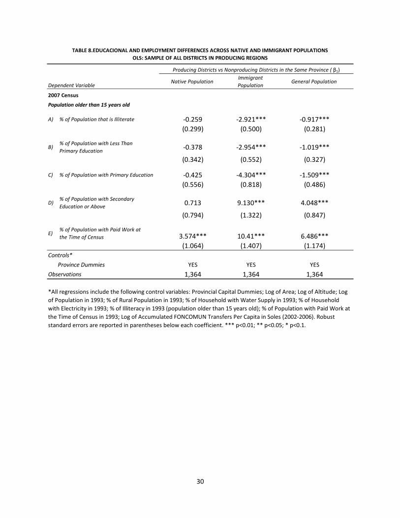
30
Dependent VariableNative Population
Immigrant
PopulationGeneral Population
2007 Census
Population older than 15 years old
A) % of Population that is Illiterate -0.259 -2.921*** -0.917***
(0.299) (0.500) (0.281)
B)% of Population with Less Than
Primary Education-0.378 -2.954*** -1.019***
(0.342) (0.552) (0.327)
C) % of Population with Primary Education -0.425 -4.304*** -1.509***
(0.556) (0.818) (0.486)
D)% of Population with Secondary
Education or Above0.713 9.130*** 4.048***
(0.794) (1.322) (0.847)
E)% of Population with Paid Work at
the Time of Census 3.574*** 10.41*** 6.486***
(1.064) (1.407) (1.174)Controls*
Province Dummies YES YES YES
Observations 1,364 1,364 1,364
TABLE 8.EDUCACIONAL AND EMPLOYMENT DIFFERENCES ACROSS NATIVE AND IMMIGRANT POPULATIONS
OLS: SAMPLE OF ALL DISTRICTS IN PRODUCING REGIONS
Producing Districts vs Nonproducing Districts in the Same Province ( β1)
*All regressions include the following control variables: Provincial Capital Dummies; Log of Area; Log of Altitude; Log
of Population in 1993; % of Rural Population in 1993; % of Household with Water Supply in 1993; % of Household
with Electricity in 1993; % of Illiteracy in 1993 (population older than 15 years old); % of Population with Paid Work at
the Time of Census in 1993; Log of Accumulated FONCOMUN Transfers Per Capita in Soles (2002-2006). Robust
standard errors are reported in parentheses below each coefficient. *** p<0.01; ** p<0.05; * p<0.1.

31
Type Source
Outcome Variables
Average Per Capita Monthly Consumption Expenditures in 2007 (Soles)
Poverty headcount index: Percent of Population under Poverty Line in 2007
The poverty line is the minimal amount of money needed by an individual to buy goods and services to satisfy basic needs. The poverty line varies by
Region and urban/rural geographic areas.
Extreme poverty headcount index: Percent of Population under Extreme Poverty Line in 2007
The extreme poverty line is the minimal amount of money needed by an individual to satisfy basic food needs. The extreme poverty line varies by
Region and urban/rural geographic areas.
Gini Coefficient of Consumption Expenditure in 2007
Regressors
1993 Control Variables 1993 Census
Producing Districts
Dummy variable that takes the value of one for all districts where there was (tax paying) production of any mineral (mainly copper, gold, and silver)
between 2002 and 2006
Nonproducing districts in Producing Provinces
Dummy variable that takes the value of one for Non-Producing Districts in a province where there is at least one Producing District.
Districts in Nonproducing Provinces
Dummy variable that takes the value of one for Non-Producing Districts in a Non-Producing Province in a Region where there is at least one Producing
District.
Value of Mineral Production in Producing District
Accumulated value of mineral production by all mining facilities within a district for the period 2002-2006. Quantity of mineral production is reported
annually by the Ministry of Energy and Mining (MINEM). Mineral prices are the annual average dollar prices per mineral reported by MINEM. Dollar
values are converted into Peruvian Soles using average exchange rates, then divided by the CPI to adjust for inflation, and finally added over 2002-06.
Value of Mineral Production in Producing Provinces
Sum of the value of production across all districts in a producing province for 2002-2006 in (constant price) Soles.
Foncomun
Accumulated revenues from the Foncomun between 2002-2006 in (constant price) Soles.
Mining Canon
Accumulated revenues from the Mining Canon for 2002-2006 in (constant price) Soles.
Administrative
Data
Peruvian Ministry of
Economy and Finance
Administrative
Data
Peruvian Ministry of
Energy and Mining
(MINEM)
Administrative
Data
Peruvian Ministry of
Energy and Mining
Administrative
Data
Peruvian Ministry of
Economy and Finance
Administrative
Data
Peruvian Ministry of
Energy and Mining
(MINEM)
National Statistical
Institute (INEI)
Administrative
Data
Peruvian Ministry of
Energy and Mining
(MINEM)
Administrative
Data
Peruvian Ministry of
Energy and Mining
2007 Poverty
Map
National Statistical
Institute (INEI)
2007 Poverty
Map
National Statistical
Institute (INEI)
Appendix Table A1. Variables Definitions and Sources
2007 Poverty
Map
National Statistical
Institute (INEI)
2007 Poverty
Map
National Statistical
Institute (INEI)

32
(1) (2) (3)
Producing
Districts
Nonproducing
Districts in
Producing
Provinces
Districts in
Nonproducing
Provinces
Outcome Variables
Average Per Capita Monthly Expenditures in 2007 (Soles) 339.57 281.36 214.60
(462.79) (1,102.69) (112.09)
% of Population under Poverty Line 52.92 60.46 63.66
(22.67) (21.49) (21.97)
% of Population under Extreme Poverty Line 23.29 29.74 31.13
(20.00) (20.81) (19.92)
Gini Coefficient (%) 29.86 28.71 28.42-3.60 -3.67 -4.18
Regressors
Altitude (meters) 2,812.33 2,821.69 2,600.40
(1,232.11) (994.06) (1,219.31)
Area (square kilometers) 551.17 333.09 433.11
(463.18) (432.08) (1,171.17)
Provincial Capital Dummy 0.11 0.08 0.11
(0.31) (0.27) (0.32)
Log of Population in 1993 8.45 7.81 8.43
(1.15) (1.12) (1.08)
% of Rural Population in 1993 54.30 57.55 65.01
(31.56) (28.01) (28.74)
% of Household with Water Supply in 1993 22.63 21.50 18.85
(21.39) (21.19) (20.90)
% of Households without Electricity in 1993 66.28 77.57 76.53
(31.45) (27.11) (27.91)
% of Population that is illiterate in 1993 (population older than 15 years old) 20.44 22.73 26.40
(12.76) (13.33) (13.70)
% of Population with Paid Work at the Time of Census in 1993 29.59 29.04 27.08
(8.07) (8.76) (6.91)
Accumulated Mineral Production Per Capita Within District In Soles (2002-2006) 284,086.10 0.00 0.00
(792,933.10) 0.00 0.00
Accumulated Foncomun per capita in Soles (2002-2006) 648.01 1,009.40 733.24
(469.24) (842.78) (701.80)
Accumulated Mining Canon per capita in soles (2002-2006) 628.59 375.29 177.41
(1,817.60) (1,213.66) (336.07)
Observations 104 563 697
APPENDIX TABLE A2. SUMMARY STATISTICS
COMPARISON OF MEANS OF OUTCOME VARIABLES AND REGRESSORS BY GROUPS (Standard deviations in parentheses)