SPATIAL MODELING IN TRANSPORTATION

by

Simon P. Anderson Department of Economics

University of Virginia

and

Wesley W. Wilson Department of Economics

University of Oregon and

Institute for Water Resources Army Corps of Engineers

September 2005

Chapter prepared for

The Handbook of Transportation Policy and Administration

Keywords: Spatial equilibrium, transportation, railroad, barge, welfare. _____________________ Much of this research was conducted under support from the Navigation Economic Technologies (NETS) program of the Institute for Water Resources of the Army Corps of Engineers. We gratefully acknowledge their support and comments. We especially appreciate the comments of Keith Hofseth and Kevin Hendrickson who read early versions of this chapter and provided a number of useful comments.

1. INTRODUCTION Evaluations of alternative transportation infrastructure improvements necessitate the

evaluation of equilibrium outcomes both with and without the improvements across the

alternatives. Transportation, however, is a derived demand. That is, it is directly linked

to the products transported and, hence, depends on the spatial differences in the origin

and terminal locations. The products travel from origin to destination over transportation

networks and geographic space. The transportation may be provided by different modes

that may compete with each other or may be essential to completing a service, and,

therefore, have both substitution and complementarities across modes. There are few

models that have the capacity to integrate some or all of these factors into an equilibrium

framework.

In this chapter, we describe the Samuelson (1952) and Takayama-Judge (1964)

model (S-TJ model) and then add a transportation market to the model. We then develop

a “full spatial” equilibrium model in which mode choices drive modal demand functions.

The chapter concludes with an application. Specifically, the Army Corps of Engineers

use a model that is comparable in many respects to the S-TJ model. We first describe this

model and then point to differences in welfare measurement between this model and the

full spatial model. The general finding of this research is that there are substantial

differences in the two models. These differences arise from the S-TJ model’s assumption

that geographic dimensions of the regions are fixed. In the full spatial model, the regions

are endogenous and depend on the costs of transportation.

Samuelson (1952) and Takayama and Judge (1964) develop a model of trade over

space. In this model, there are multiple regions that both demand and/or supply a product.

1

If transportation costs are too high or if transportation is not possible, equilibrium is

established by standard local supply and demand conditions. In such a case, there are

price differences in the commodity across the regions. Transportation allows these price

differences to be arbitraged. In equilibrium, either prices differ in the two markets by a

transportation cost or else no trade occurs. Commonly, these models treat transportation

as given. However, the model is can be fully endogenized through the addition of

transportation supply. In the model developed in the next section, we solve the model

for two regions with no trade, with trade at a given transportation rate, and then complete

the model with the addition of transportation supply. In transportation planning, the key

policy variables underpin the transportation supply function. Specifically, improvements

to the transportation infrastructure reduce the cost of providing transportation. The

reductions in cost reflect a shift down in the supply function, reducing the transportation

rate, and facilitating trade between regions.

In the S-TJ framework, the regions themselves are exogenously fixed in the sense

that the size of the regions are unaffected by the transportation rate. In some cases, such

an assumption is perfectly suited to modeling trade and transportation policy. For

example, this applies to trade between countries and isolated regions wherein suppliers

(transportation demanders) have no other options. However, in most transportation

settings, regions are adjacent to one another. The total supply of a product is an

aggregation of suppliers distributed throughout the regions. Transportation policy may

impact the decisions of the individual suppliers on the routes or modes they choose.

Since, for any given region, suppliers are spatially distributed, transportation policy

affects the size of the region over which suppliers are aggregated to form the region’s

2

supply function. Thus, the size of the region and, therefore, the level of supply are

determined endogenously in the equilibrium. The welfare consequences of an

improvement to the transportation infrastructure in the S-TJ setting does not include the

shifts in the regional borders and may therefore overestimate the welfare impact of

improvements to the transportation infrastructure.

A full spatial model is developed as an alternative description that explicityly

addresses this point. In this model, suppliers of a product are taken to be spatially

distributed over a region. The individual suppliers are taken as the demanders of

transportation. They choose a mode and routing option to get the product to market. The

modal splits and the routing options transcend into regional supplies of a product and,

hence, into transportation demands. As in our development of the S-TJ model,

transportation equilibrium obtains through the summation of modal supplies and

completes the model. Also, in parallel with our development of S-TJ, improvements to

the transportation infrastructure reduce the costs of transportation services. This

reduction in costs facilitates trade between regions.

The chapter concludes with an illustration. While a number of differing

infrastructure improvements can be made with modest modifications to the model, the

particular improvement analyzed is a lock improvement. Locks are an essential

component of the inland waterway system and are necessary for navigation. The locks

and dams in the inland waterway system are managed by the Army Corps of Engineers

(ACE). In determining whether improvements are made and the type of improvements,

ACE evaluates the costs and benefits of alternatives. Their methodology to determine the

costs and benefits of lock improvements has come under tremendous recent scrutiny, and

3

a core criticism centers on the lack of an appropriate spatial equilibrium model. Their

model uses a fixed region akin to S-TJ and demand structures that are perfectly inelastic

to a threshold rate. In our application, we describe the model used by ACE along with

comparisons to S-TJ. We then use the full spatial model to compare the welfare

consequences of lock improvements against ACE's methodology. This comparison

identifies differences that could seriously impact the calculations of net benefits accruing

to transportation infrastructure improvements.

2. THE SAMUELSON AND TAKAYAMA-JUDGE APPROACH

In this section, we briefly review the classic spatial model of Samuelson (1952) and

Takayama and Judge (1964).1 In the S-T-J model, there is a set of regions trading a good.

Each region is endowed with a set of demand and supply functions. If markets are

completely separated (i.e., no trade is allowed, or else is prohibitively costly), markets are

cleared in the usual way in equilibrium. That is, demand and supply functions are

equated for each region to give equilibrium prices and quantities.

Transportation, however, if not too costly, allows trade to occur between regions

and causes price differences between regions to be arbitraged. To illustrate this point,

suppose that there were no transportation costs. The prices in the regions then must be

the equal in equilibrium. No difference can be sustained because goods would flow from

1Samuelson in turn drew on Enke (1951). Enke proposed the problem of determining spatial transportation patterns (under a linear demand system). His solution was inspired by the analogue to the problem in an electric system, and he could measure equilibrium prices and quantities with voltmeters and ammeters. Samuelson (1952) then set up and solved the problem as a linear programming problem. Takayama and Judge (1964) converted the Samuelson-Enke problem into a quadratic programming problem and found the solution algorithm (still for linear demands).

4

any low price region to a higher price one if transportation were costless. With costly

transportation, differential prices will reflect transportation costs: transportation will

arbitrage excessive price differences between the regions.

2.1 An Illustrative Example - Prohibitive Transportation Costs

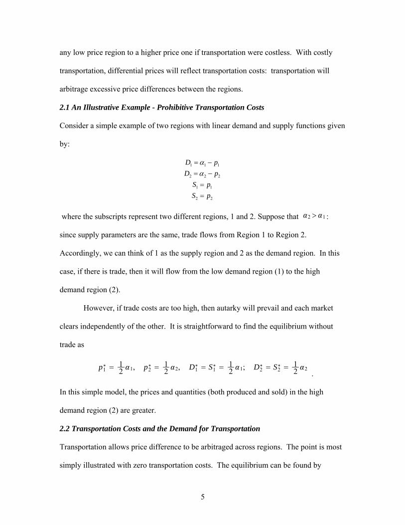
Consider a simple example of two regions with linear demand and supply functions given

by: 1 1 1

2 2

1 1

2 2

2

D pD p

S pS p

αα

= −= −==

where the subscripts represent two different regions, 1 and 2. Suppose that :

since supply parameters are the same, trade flows from Region 1 to Region 2.

Accordingly, we can think of 1 as the supply region and 2 as the demand region. In this

case, if there is trade, then it will flow from the low demand region (1) to the high

demand region (2).

2 1

However, if trade costs are too high, then autarky will prevail and each market

clears independently of the other. It is straightforward to find the equilibrium without

trade as

p1∗ 1

2 1, p2∗ 1

2 2, D1∗ S1

∗ 12 1; D2

∗ S2∗ 1

2 2.

In this simple model, the prices and quantities (both produced and sold) in the high

demand region (2) are greater.

2.2 Transportation Costs and the Demand for Transportation

Transportation allows price difference to be arbitraged across regions. The point is most

simply illustrated with zero transportation costs. The equilibrium can be found by

5

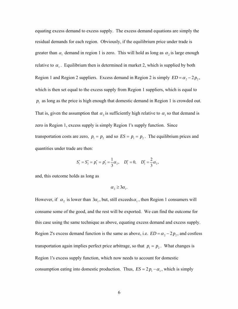
equating excess demand to excess supply. The excess demand equations are simply the

residual demands for each region. Obviously, if the equilibrium price under trade is

greater than 1α demand in region 1 is zero. This will hold as long as 2α is large enough

relative to 1α . Equilibrium then is determined in market 2, which is supplied by both

Region 1 and Region 2 suppliers. Excess demand in Region 2 is simply 2 22ED pα= − ,

which is then set equal to the excess supply from Region 1 suppliers, which is equal to

1p as long as the price is high enough that domestic demand in Region 1 is crowded out.

That is, given the assumption that 2α is sufficiently high relative to 1α so that demand is

zero in Region 1, excess supply is simply Region 1's supply function. Since

transportation costs are zero, 1 2p p= and so 1ES p p2= = . The equilibrium prices and

quantities under trade are then:

1 2 1 2 2 1 2 21 2, 0, , 3 3

S S p p D Dα α∗ ∗ ∗ ∗ ∗ ∗= = = = = =

and, this outcome holds as long as

2 13 .α α≥

However, if 2α is lower than 13α , but, still exceeds 1α , then Region 1 consumers will

consume some of the good, and the rest will be exported. We can find the outcome for

this case using the same technique as above, equating excess demand and excess supply.

Region 2's excess demand function is the same as above, i.e. 2 2ED p2α= − , and costless

transportation again implies perfect price arbitrage, so that 1 2p p= . What changes is

Region 1's excess supply function, which now needs to account for domestic

consumption eating into domestic production. Thus, 12ES p 1α= − , which is simply

6

domestic supply minus domestic demand. Pulling these equations together yields the

equilibrium prices and quantities under trade as:

1 2 1 2 2 11 2 1 2 1 2

3 3, , , 4 4 4

S S p p D Dα α α α α α∗ ∗ ∗ ∗ ∗ ∗+ − −= = = = = =

that holds as long as

[ ]2 1 1,3 .α α α∈

Transportation, however, is costly. Let t represent the cost per unit of the good

transported. For now, consider the case of one mode providing transportation from

Region 1 to Region 2. The excess demand and excess supply equations above still apply

to the case of costly transportation, but transportation can no longer arbitrage prices to be

the same. Instead, arbitrage implies that price differences cannot exceed the transport

cost. That is, the price differences are bounded by the constraint 2 1p p t≤ + . If there is

trade in equilibrium, this holds with equality (so 2 1p p t= + ) and differential prices

simply reflect the cost of transporting the good to the demand region. On the other hand,

if prices are closer together than t ( 2 1p p t< + ) there can be no trade since arbitrage

cannot be profitable. The equilibrium types then are like the ones we have already

described: if transport costs are too large, the autarkic equilibrium prevails. For lower

costs, there is trade, and the supply region will export its total production only if its

domestic demand is weak relative to that in the demand region.

The autarky regime is the simplest to describe. As demonstrated above, autarky

prices are 1 112

p α∗ = and 212

p 2α∗ = , so that autarky remains as long as the price

7

difference is less than the transportation cost. Equivalently, 2 1 2tα α− ≤ means there will

be no trade.

In the case of lower transport cost but weak demand in the supply region, then

demand in the low demand Region, 1, is zero. To characterize this case, we equate

excess demand and excess supply so 2 22 pα − = 1p and use the price difference equation

given by 2 1p p t= + . Solving, the result is 2 21 3

tp α −∗ = and 22 3

tp α +∗ = . Each region's

domestic production equals its domestic supply, and quantity consumed in Region 1 is

zero, while in Region 2 it is given by the demand curve as 22

23

tD α∗ −= . For this regime

to be pertinent, it must be the case that 1p 1α∗ ≥ , otherwise there would be positive

consumption in the supply region. This condition is 2 2 3t 1α α− ≥ . Notice that the

quantity transported from 1 to 2 is the full quantity produced in 1, namely, 2 23

tα − . This

equation also forms the demand for transportation, and is a decreasing function of t.

For low transport cost and relatively strong Region 1 demand, not all Region 1's

production will be exported. Equating excess demand and excess supply, in this case,

implies 2 2 12 2p p 1α α− = − , and, again, the price difference equation 2 1p p= + t holds.

Solving these equations gives 1 2 21 4

tp α α+ −∗ = and 1 2 22 4

tp α α+ +∗ = : Once again, these are also

the respective expressions for the domestic supplies, 1S ∗ and 2S ∗ respectively. The

quantities consumed are 1D∗ = 1 23 24

tα α− + and 1 23 22 4 ,tD α α− + −∗ = respectively.2 From the first

S S D∗ ∗ ∗+ = +

2It is readily checked that total production equals total consumption, i.e.,

1 2 1 2D∗ 1 22

α α+= .

8

of these, it is clear that we need the condition 13 2t 2α α+ > to hold in order for to

indeed be positive. The quantity transported in this case is given by

1D∗

2 1( )2T tα α−= − , and

constitutes the demand function for transportation.

The results of both cases are similar. Specifically, as demand in the excess

demand region grows, quantities transported increase, and, as the transportation rate

increases, quantities transported fall. In the latter case, as demand in the excess supply

region grows (i.e., 1α increases), less is transported.

The model, to this point, has the cost of providing transportation as exogenous. It

merely indicates the interrelationship of demand and supply conditions in each region

without and with transportation charges. We address this issue in the remainder of this

section.

2.3 Transportation Market Equilibrium

There is considerable interest in modeling equilibrium in the transportation market as an

end in itself. The models in the previous sub-sections illustrate the construction of

demand for transportation. In this sub-section, we add in the supply of transportation. In

the literature, transportation firms are typically taken as price-takers. The supply of

transportation then emanates from cost functions. In the simplest case, suppose that costs

are a constant ( c ) per-unit of output shipped. The equilibrium transport rate t is simply

this cost (i.e., t per unit shipped). Any improvement in cost conditions (a reduction in

) then reduces transportation costs and facilitates trade between the regions.

c=

c

In a slightly more complicated case, suppose that the marginal cost of a

transportation firm is linearly increasing in output shipped i.e., MC cq= . If there are N

9

such providers, then transportation supply function is given by S tT Nc

= . In the context

of the demand models established above, transportation demand and supply are set equal

to find equilibrium. An improvement in cost conditions of transportation suppliers

increases transportation supply and reduces the transportation rate. This, in turn (and as

above) facilitates trade between the two regions.

3. FULL SPATIAL MODEL OF RAIL AND BARGE COMPETITION

Development of the full spatial model requires some detail on the locations of shippers,

the geography of the transportation network, and the options available to shippers. To

this end, we follow our previous work (Anderson and Wilson (2004; 2005)). In what

follows, we take shippers to be the suppliers of the product which is shipped. These

shippers are located over a space. Shippers ship to a single terminal market and can ship

by rail, barge or a combination of truck and barge. We assume that commodities flow to

a single terminal market.3 Further, the present case is confined to rail and truck-barge

alternatives. That is, shippers cannot use truck only as an alternative.4

The river-canal system runs from North to South, and terminates at the terminal

market which may reflect a final transshipment port (e.g., New Orleans). Let the East-

West distance from the river be in the direction, and let the North-South direction up

and down the river be denoted by . The river is divided up into “pools”. A pool is

a body of water between fixed points. For our purposes, and as discussed in greater detail

below, ACE planning purposes, pools are bodies of water between two locks.

x

0y ≥

3 As demonstrated in previous work, the model can be adapted to allow for multiple terminal markets (Anderson and Wilson (2005)). 4 This development is made for convenience and exposition, but, in Anderson and Wilson (2004), the assumption is relaxed and analyzed.

10

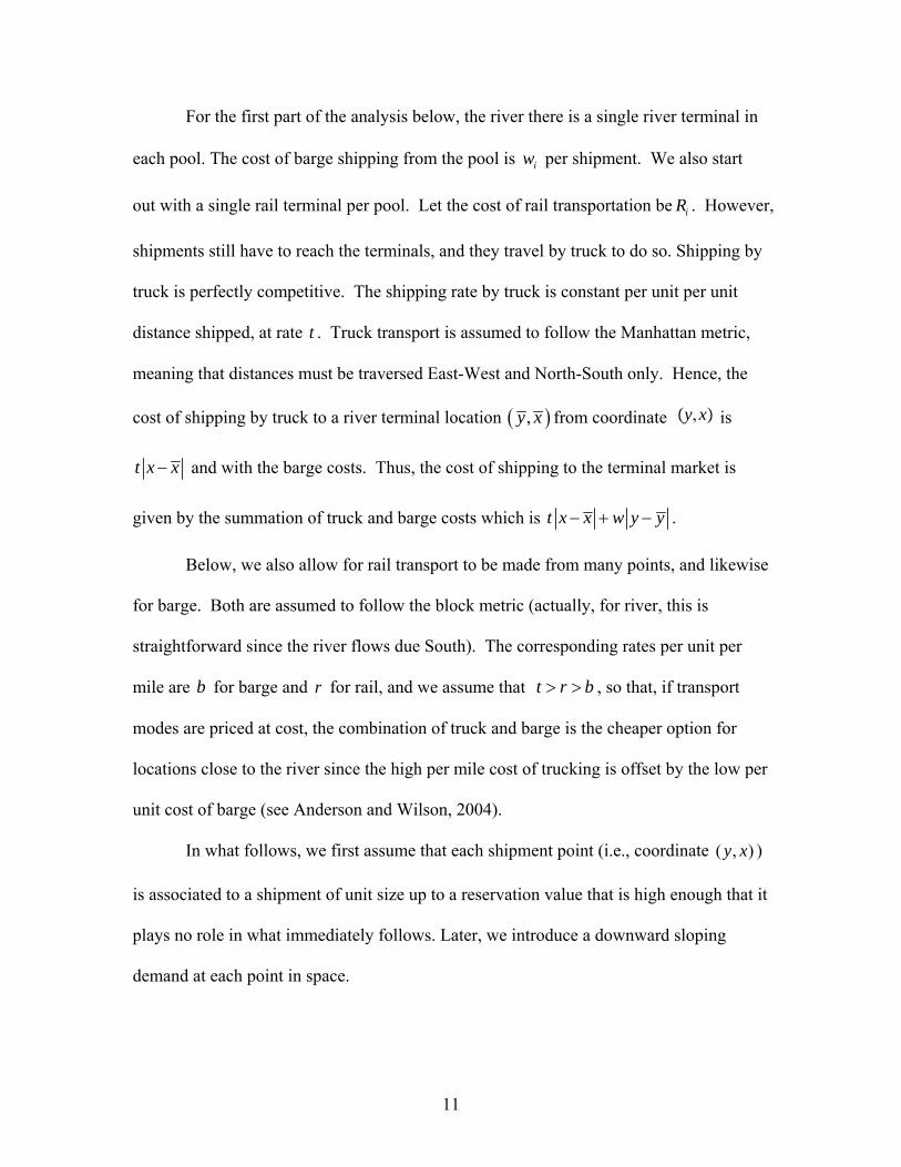
For the first part of the analysis below, the river there is a single river terminal in

each pool. The cost of barge shipping from the pool is per shipment. We also start

out with a single rail terminal per pool. Let the cost of rail transportation be

iw

iR . However,

shipments still have to reach the terminals, and they travel by truck to do so. Shipping by

truck is perfectly competitive. The shipping rate by truck is constant per unit per unit

distance shipped, at rate t . Truck transport is assumed to follow the Manhattan metric,

meaning that distances must be traversed East-West and North-South only. Hence, the

cost of shipping by truck to a river terminal location ( ),y x from coordinate y,x is

t x x− and with the barge costs. Thus, the cost of shipping to the terminal market is

given by the summation of truck and barge costs which is t x x w y y− + − .

Below, we also allow for rail transport to be made from many points, and likewise

for barge. Both are assumed to follow the block metric (actually, for river, this is

straightforward since the river flows due South). The corresponding rates per unit per

mile are for barge and for rail, and we assume that t r , so that, if transport

modes are priced at cost, the combination of truck and barge is the cheaper option for

locations close to the river since the high per mile cost of trucking is offset by the low per

unit cost of barge (see Anderson and Wilson, 2004).

b r b> >

In what follows, we first assume that each shipment point (i.e., coordinate )

is associated to a shipment of unit size up to a reservation value that is high enough that it

plays no role in what immediately follows. Later, we introduce a downward sloping

demand at each point in space.

( , )y x

11

3.1 Single river terminal per pool, single rail terminal

A focal point of this chapter is to develop a full spatial model from which welfare

changes from a transportation infrastructure improvement can be evaluated and compared

with ACE modeling efforts. To illustrate the restrictive assumptions implicit in the ACE

and S-TJ models, we first give a set of conditions that when applied to the full spatial

model generates the fixed region assumption within a spatial context. To fix regions and

satisfy the properties of the S-TJ and ACE approaches, there are a number of assumptions

which can be imposed on the model. These are:

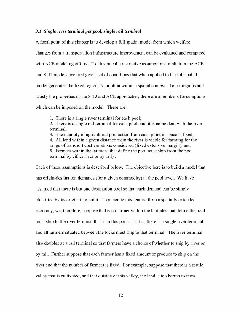
1. There is a single river terminal for each pool; 2. There is a single rail terminal for each pool, and it is coincident with the river terminal; 3. The quantity of agricultural production from each point in space is fixed; 4. All land within a given distance from the river is viable for farming for the range of transport cost variations considered (fixed extensive margin); and 5. Farmers within the latitudes that define the pool must ship from the pool terminal by either river or by rail) .

Each of these assumptions is described below. The objective here is to build a model that

has origin-destination demands (for a given commodity) at the pool level. We have

assumed that there is but one destination pool so that each demand can be simply

identified by its originating point. To generate this feature from a spatially extended

economy, we, therefore, suppose that each farmer within the latitudes that define the pool

must ship to the river terminal that is in this pool. That is, there is a single river terminal

and all farmers situated between the locks must ship to that terminal. The river terminal

also doubles as a rail terminal so that farmers have a choice of whether to ship by river or

by rail. Further suppose that each farmer has a fixed amount of produce to ship on the

river and that the number of farmers is fixed. For example, suppose that there is a fertile

valley that is cultivated, and that outside of this valley, the land is too barren to farm.

12

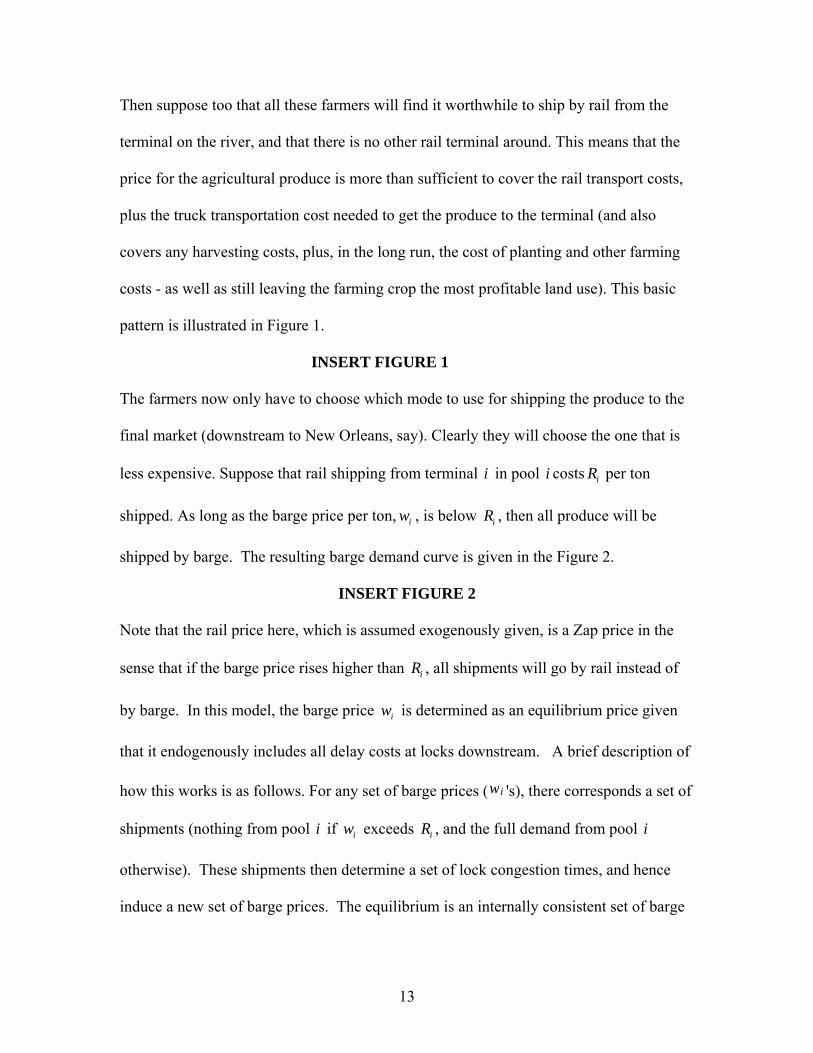
Then suppose too that all these farmers will find it worthwhile to ship by rail from the

terminal on the river, and that there is no other rail terminal around. This means that the

price for the agricultural produce is more than sufficient to cover the rail transport costs,

plus the truck transportation cost needed to get the produce to the terminal (and also

covers any harvesting costs, plus, in the long run, the cost of planting and other farming

costs - as well as still leaving the farming crop the most profitable land use). This basic

pattern is illustrated in Figure 1.

INSERT FIGURE 1

The farmers now only have to choose which mode to use for shipping the produce to the

final market (downstream to New Orleans, say). Clearly they will choose the one that is

less expensive. Suppose that rail shipping from terminal i in pool costsi iR per ton

shipped. As long as the barge price per ton, , is below iw iR , then all produce will be

shipped by barge. The resulting barge demand curve is given in the Figure 2.

INSERT FIGURE 2

Note that the rail price here, which is assumed exogenously given, is a Zap price in the

sense that if the barge price rises higher than iR , all shipments will go by rail instead of

by barge. In this model, the barge price is determined as an equilibrium price given

that it endogenously includes all delay costs at locks downstream. A brief description of

how this works is as follows. For any set of barge prices (

iw

wi 's), there corresponds a set of

shipments (nothing from pool i if exceeds iw iR , and the full demand from pool i

otherwise). These shipments then determine a set of lock congestion times, and hence

induce a new set of barge prices. The equilibrium is an internally consistent set of barge

13

prices (a fixed point in technical terms) such that the barge prices induce exactly the set

of shipments that give rise to the barge prices.

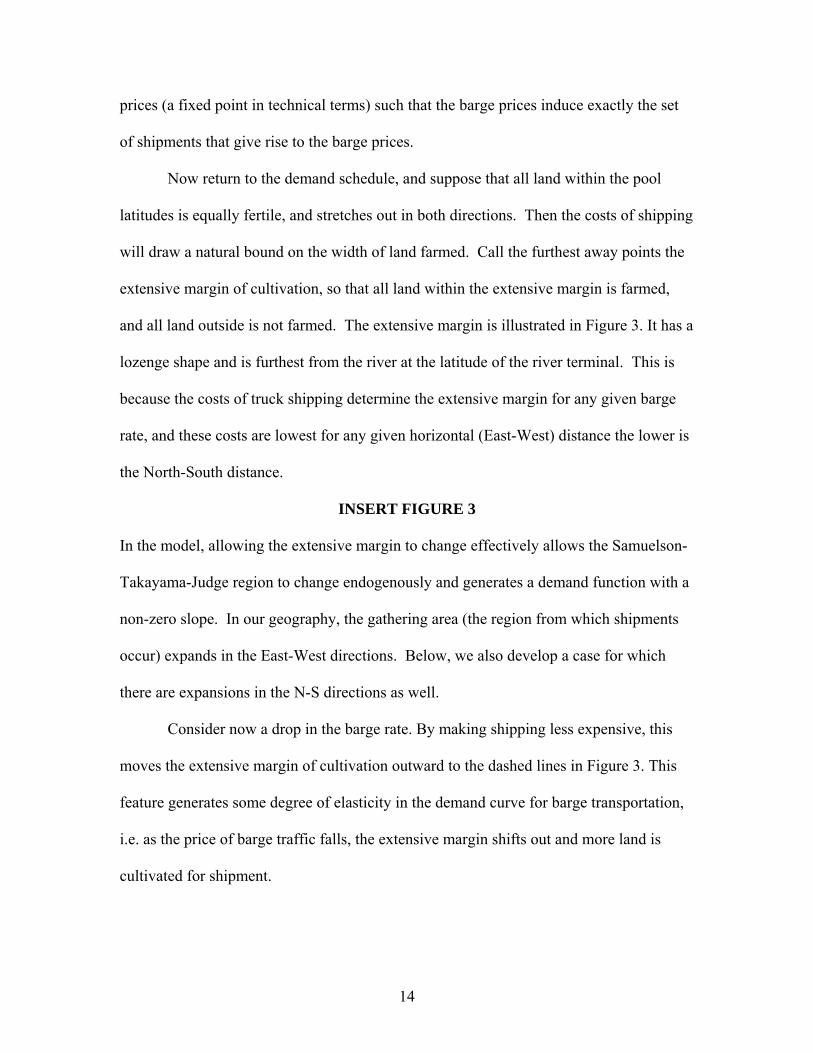
Now return to the demand schedule, and suppose that all land within the pool

latitudes is equally fertile, and stretches out in both directions. Then the costs of shipping

will draw a natural bound on the width of land farmed. Call the furthest away points the

extensive margin of cultivation, so that all land within the extensive margin is farmed,

and all land outside is not farmed. The extensive margin is illustrated in Figure 3. It has a

lozenge shape and is furthest from the river at the latitude of the river terminal. This is

because the costs of truck shipping determine the extensive margin for any given barge

rate, and these costs are lowest for any given horizontal (East-West) distance the lower is

the North-South distance.

INSERT FIGURE 3

In the model, allowing the extensive margin to change effectively allows the Samuelson-

Takayama-Judge region to change endogenously and generates a demand function with a

non-zero slope. In our geography, the gathering area (the region from which shipments

occur) expands in the East-West directions. Below, we also develop a case for which

there are expansions in the N-S directions as well.

Consider now a drop in the barge rate. By making shipping less expensive, this

moves the extensive margin of cultivation outward to the dashed lines in Figure 3. This

feature generates some degree of elasticity in the demand curve for barge transportation,

i.e. as the price of barge traffic falls, the extensive margin shifts out and more land is

cultivated for shipment.

14

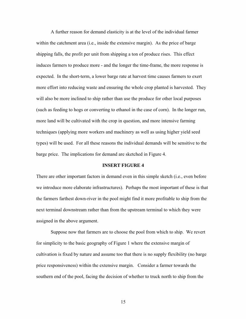
A further reason for demand elasticity is at the level of the individual farmer

within the catchment area (i.e., inside the extensive margin). As the price of barge

shipping falls, the profit per unit from shipping a ton of produce rises. This effect

induces farmers to produce more - and the longer the time-frame, the more response is

expected. In the short-term, a lower barge rate at harvest time causes farmers to exert

more effort into reducing waste and ensuring the whole crop planted is harvested. They

will also be more inclined to ship rather than use the produce for other local purposes

(such as feeding to hogs or converting to ethanol in the case of corn). In the longer run,

more land will be cultivated with the crop in question, and more intensive farming

techniques (applying more workers and machinery as well as using higher yield seed

types) will be used. For all these reasons the individual demands will be sensitive to the

barge price. The implications for demand are sketched in Figure 4.

INSERT FIGURE 4

There are other important factors in demand even in this simple sketch (i.e., even before

we introduce more elaborate infrastructures). Perhaps the most important of these is that

the farmers farthest down-river in the pool might find it more profitable to ship from the

next terminal downstream rather than from the upstream terminal to which they were

assigned in the above argument.

Suppose now that farmers are to choose the pool from which to ship. We revert

for simplicity to the basic geography of Figure 1 where the extensive margin of

cultivation is fixed by nature and assume too that there is no supply flexibility (no barge

price responsiveness) within the extensive margin. Consider a farmer towards the

southern end of the pool, facing the decision of whether to truck north to ship from the

15

pool i or whether to truck south, and ship from the terminal in the next pool down, pool

. We naturally expect the barge rate to be lower further south ( ) because a

smaller distance is traversed on the river and one less lock is crossed. The farmer must,

therefore, weigh the costs of trucking to the two alternative terminals. The indifferent

farmer defines the market boundary for the catchment areas of the two pools. Those

farmers further north of the boundary will ship to the pool i terminal, and conversely,

those further south will ship to the pool

1i − 1iw w− < i

1i − terminal.5

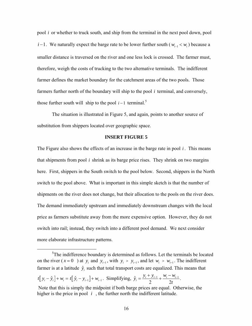
The situation is illustrated in Figure 5, and again, points to another source of

substitution from shippers located over geographic space.

INSERT FIGURE 5

The Figure also shows the effects of an increase in the barge rate in pool . This means

that shipments from pool i shrink as its barge price rises. They shrink on two margins

here. First, shippers in the South switch to the pool below. Second, shippers in the North

switch to the pool above. What is important in this simple sketch is that the number of

shipments on the river does not change, but their allocation to the pools on the river does.

The demand immediately upstream and immediately downstream changes with the local

price as farmers substitute away from the more expensive option. However, they do not

switch into rail; instead, they switch into a different pool demand. We next consider

more elaborate infrastructure patterns.

i

5The indifference boundary is determined as follows. Let the terminals be located

on the river ( ) at and 0x = iy 1iy − , with iy > 1iy − , and let iw > 1iw − . The indifferent farmer is at a latitude such that total transport costs are equalized. This means that ˆiy

[ ]ˆi i it y y w− + = [ ]1ˆi i it y y w−− + 1− . Simplifying, 1 1ˆ .2 2

i i i ii

y y w wyt

− −+ −= +

Note that this is simply the midpoint if both barge prices are equal. Otherwise, the higher is the price in pool i , the further north the indifferent latitude.

16

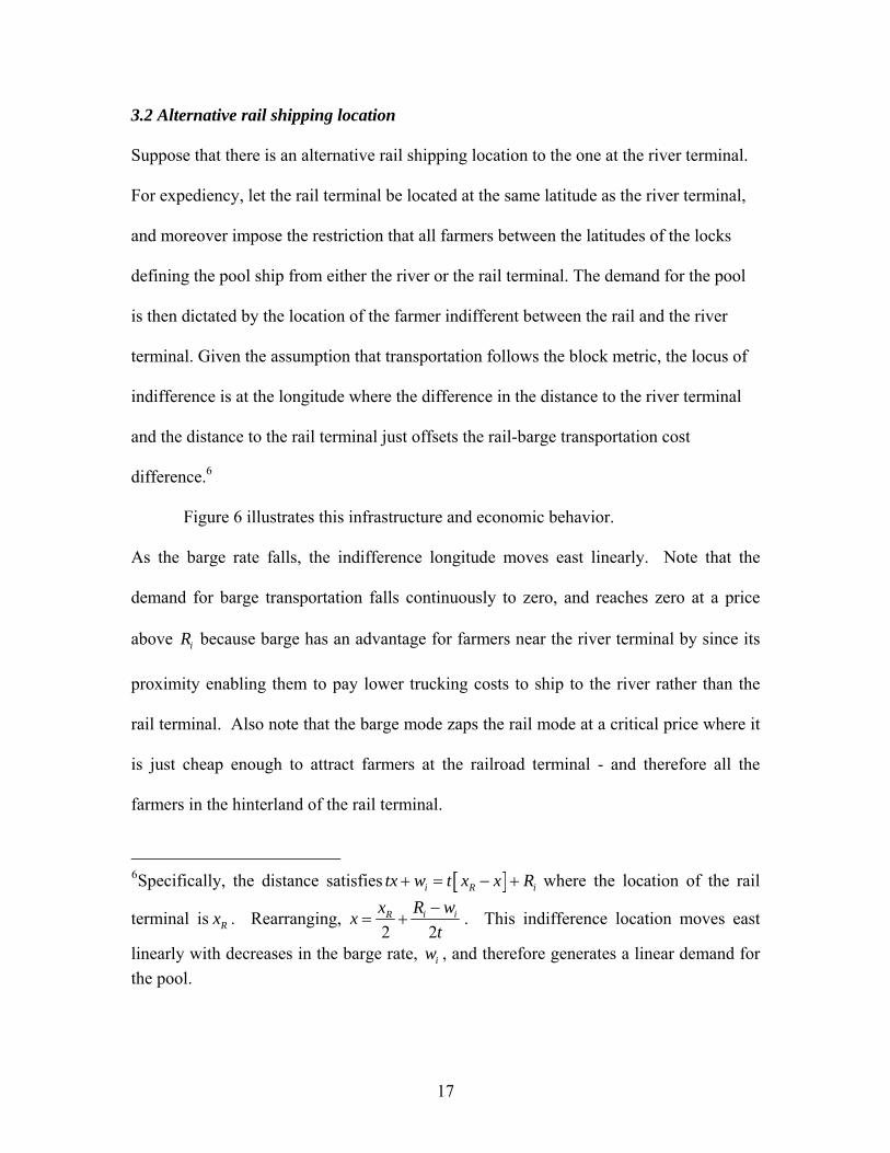
3.2 Alternative rail shipping location

Suppose that there is an alternative rail shipping location to the one at the river terminal.

For expediency, let the rail terminal be located at the same latitude as the river terminal,

and moreover impose the restriction that all farmers between the latitudes of the locks

defining the pool ship from either the river or the rail terminal. The demand for the pool

is then dictated by the location of the farmer indifferent between the rail and the river

terminal. Given the assumption that transportation follows the block metric, the locus of

indifference is at the longitude where the difference in the distance to the river terminal

and the distance to the rail terminal just offsets the rail-barge transportation cost

difference.6

Figure 6 illustrates this infrastructure and economic behavior.

As the barge rate falls, the indifference longitude moves east linearly. Note that the

demand for barge transportation falls continuously to zero, and reaches zero at a price

above iR because barge has an advantage for farmers near the river terminal by since its

proximity enabling them to pay lower trucking costs to ship to the river rather than the

rail terminal. Also note that the barge mode zaps the rail mode at a critical price where it

is just cheap enough to attract farmers at the railroad terminal - and therefore all the

farmers in the hinterland of the rail terminal.

6Specifically, the distance satisfies [ ]i Rtx w t x x Ri+ = − + where the location of the rail

terminal is Rx . Rearranging, 2 2

iR iR wxxt−

= + . This indifference location moves east

linearly with decreases in the barge rate, , and therefore generates a linear demand for the pool.

iw

17

INSERT FIGURE 6

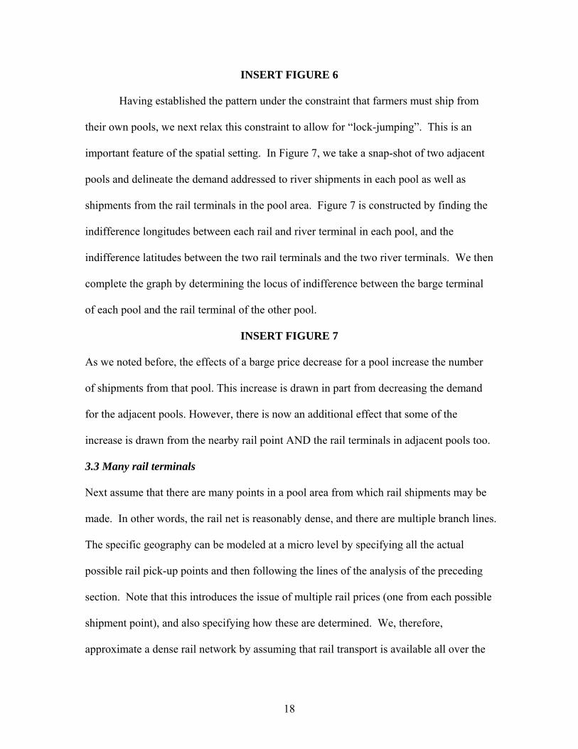
Having established the pattern under the constraint that farmers must ship from

their own pools, we next relax this constraint to allow for “lock-jumping”. This is an

important feature of the spatial setting. In Figure 7, we take a snap-shot of two adjacent

pools and delineate the demand addressed to river shipments in each pool as well as

shipments from the rail terminals in the pool area. Figure 7 is constructed by finding the

indifference longitudes between each rail and river terminal in each pool, and the

indifference latitudes between the two rail terminals and the two river terminals. We then

complete the graph by determining the locus of indifference between the barge terminal

of each pool and the rail terminal of the other pool.

INSERT FIGURE 7

As we noted before, the effects of a barge price decrease for a pool increase the number

of shipments from that pool. This increase is drawn in part from decreasing the demand

for the adjacent pools. However, there is now an additional effect that some of the

increase is drawn from the nearby rail point AND the rail terminals in adjacent pools too.

3.3 Many rail terminals

Next assume that there are many points in a pool area from which rail shipments may be

made. In other words, the rail net is reasonably dense, and there are multiple branch lines.

The specific geography can be modeled at a micro level by specifying all the actual

possible rail pick-up points and then following the lines of the analysis of the preceding

section. Note that this introduces the issue of multiple rail prices (one from each possible

shipment point), and also specifying how these are determined. We, therefore,

approximate a dense rail network by assuming that rail transport is available all over the

18

geographic space. The advantage of this approximation is to give a clearer picture of the

overall system equilibrium shipment pattern.

We retain for now the assumption that there is a single river terminal per pool.

Once again, to emphasize the demands at each pool are independent of demands in the

adjacent to pools in both the S-TJ and, as discussed below, the ACE models, we first

solve the model with the assumption that all shipments originating between the two

latitudes defining the pool must ship from that pool's river terminal if shipping is done by

the river (i.e., truck-barge is used). We then relax this assumption and let prices dictate

the pool from which farmers initiate barge movements.

As above, let t denote the cost per unit shipped per unit distance using truck.

Further, let be the cost of shipping from the river terminal in pool i . We now also

must specify how much rail shipping costs differ from different points. To accomplish

this, we shall use a block metric system just as we did above for the trucking sector.

What this means is that transportation can be viewed as following a grid network, and

distances are traversed only North-South and East-West. We suppose that the cost of rail

shipping is linear in the (block) distance shipped, at rate per unit shipped per unit

distance. Thus, we can specify shipping costs from any point in space. We know that

rail shipping is cheaper the closer to the river is the origin, as is also true for truck-barge

(since the rail traffic effectively must traverse the same East-West mileage as the truck

traffic). Rail is also cheaper the closer the origin to the destination. For barge though,

this is not true if the origin point is South of the pool river terminal. In that case, the

further South, the greater the shipping cost because a greater distance must be traveled

North by truck to reach the terminal. However, of the points north of the terminal,

iw

r

19

further South is better because it is synonymous with closer to the river terminal.

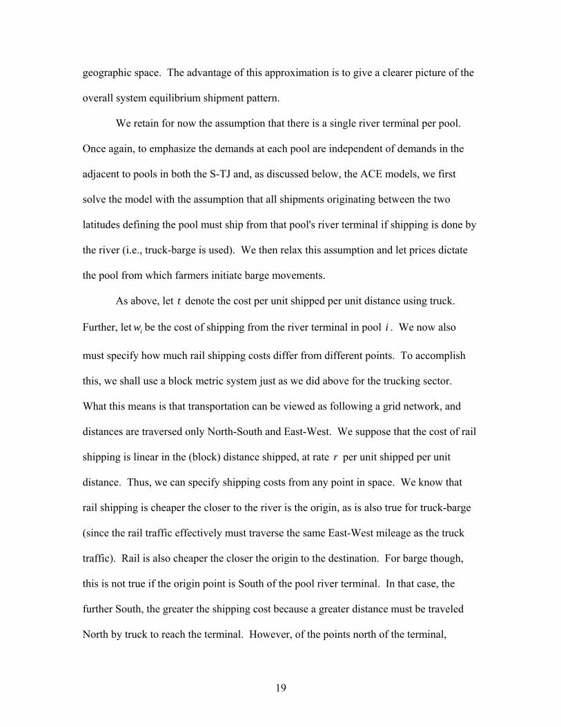
To find the catchment area for barge within the pool latitudes for this case, it

suffices to find the indifferent farmer location such that the farmer pays just as much

shipping by truck to the terminal and then by barge thereafter as he does shipping by rail

throughout. Figure 8 illustrates the resulting spatial catchment area. Notice that it reaches

furthest East at the latitude of the river terminal: this is because the relative advantage of

barge is highest there because transportation by truck needs no North-South component.

INSERT FIGURE 8

The Figure also illustrates the effects on the barge catchment area of decreasing the water

rate, .iw 7 Notice that the decrease in the barge rate causes the catchment area to expand in

a parallel fashion. This means that if the density of farmers is uniform over space, then

the demand function for the pool is a linear function of the barge rate, .iw 8

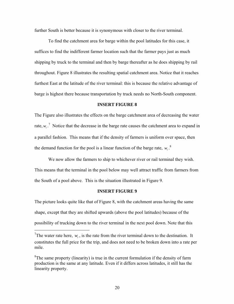
We now allow the farmers to ship to whichever river or rail terminal they wish.

This means that the terminal in the pool below may well attract traffic from farmers from

the South of a pool above. This is the situation illustrated in Figure 9.

INSERT FIGURE 9

The picture looks quite like that of Figure 8, with the catchment areas having the same

shape, except that they are shifted upwards (above the pool latitudes) because of the

possibility of trucking down to the river terminal in the next pool down. Note that this 7The water rate here, , is the rate from the river terminal down to the destination. It constitutes the full price for the trip, and does not need to be broken down into a rate per mile.

iw

8The same property (linearity) is true in the current formulation if the density of farm production is the same at any latitude. Even if it differs across latitudes, it still has the linearity property.

20

lock-jumping feature also entails there being continuity in the longitudinal boundary (as

illustrated) as we pass from one pool catchment area to the next one down. The

latitudinal boundary between two pools' catchment areas is horizontal, as given in Figure

9, because of the assumption of block distance in trucking: trucks must also travel in

North-South and East-West patterns only. While a crow-flies distance would give a more

intricate pattern, it would not fundamentally alter the qualitative result of the Figure.9

3.4 Many rail terminals and many river terminals (dense infrastructure)

The models above have assumed that there is a single river terminal per pool. In

practice, there are often several locations within a pool at which barges can be loaded.

Having just analyzed the case of many rail terminals over space, we now develop the

model for the case of many river terminals. Again, for clarity, we suppose that any point

on the river is a candidate barge-loading location. There is a difference between the case

of many rail terminals and many river terminals: in the former case, anywhere in the two-

dimensional geographic space is a potential loading point, while in the latter case the

loading points are constrained to points along the river. This means that trucks must be

used to reach the river to use barge, while rail goes directly from the point of production.

We now need to also specify the rate per unit distance traveled by barge. Call this

rate b . Barge must be used in conjunction with truck (which operates at rate t ), and so

truck-barge combines the most expensive mode (truck) with the least expensive mode

(barge). Letting the rail rate per unit per unit distance be , we assume that .

This pattern of costs ensures that both modes (rail and the joint truck-barge one) are

r t r b> >

9Using the actual road net would likely yield an intermediate pattern.

21

viable in equilibrium. Moreover, truck-barge dominates in the neighborhood of the river.

We also suppose that barge shipping entails an extra cost whenever locks are crossed:

denote the cost associated with Lock i as . ic

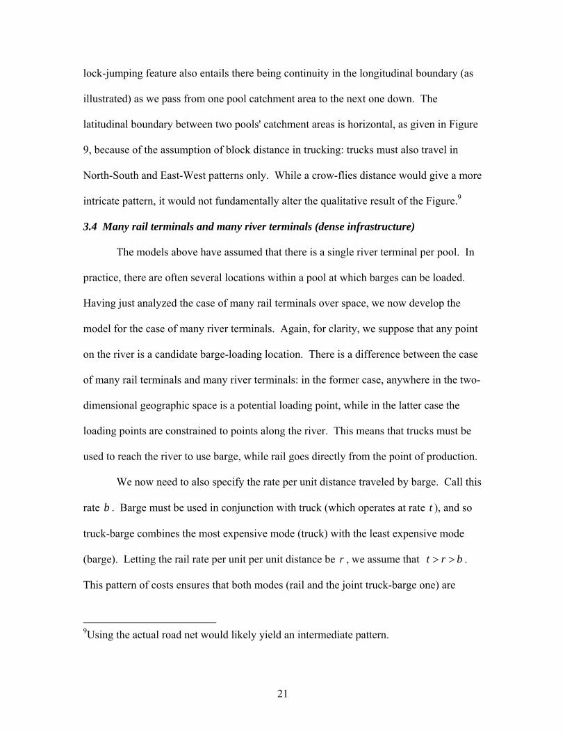
Since the terminal market is at location y 0 , x 0 , the cost of making a

shipment from a location with coordinates ( ),y x is therefore r x ry+ using rail. Using

the truck-barge mode, the cost is { }| i

ii y y

t x by c<

+ + ∑ where the summation encompasses

the total cost of traversing all locks between origin ( y ) and destination ( ). For

comparison with what has come before, we start out by maintaining the hypothesis that

each shipper must ship from his own latitude ( ) if shipping by barge. This gives rise to

the following pattern of barge shipment areas.

0

x

INSERT FIGURE 10

This Figure embodies the idea that crossing a lock adds to the cost of barge shipping.10

The existence of this cost, though, means that farmers may prefer to ship down (by truck)

below the costly lock.11 Indeed, Figure 10clearly indicates that such an arbitrage

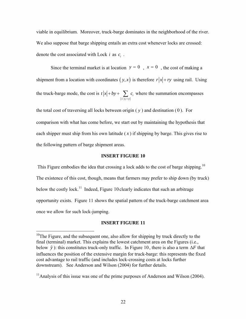
opportunity exists. Figure 11 shows the spatial pattern of the truck-barge catchment area

once we allow for such lock-jumping.

INSERT FIGURE 11

10The Figure, and the subsequent one, also allow for shipping by truck directly to the final (terminal) market. This explains the lowest catchment area on the Figures (i.e., below ): this constitutes truck-only traffic. In Figure 10 , there is also a term that influences the position of the extensive margin for truck-barge: this represents the fixed cost advantage to rail traffic (and includes lock-crossing costs at locks further downstream). See Anderson and Wilson (2004) for further details.

y F∆

11Analysis of this issue was one of the prime purposes of Anderson and Wilson (2004).

22

Notice the similarity between Figure 11 and Figure 9 , which shows the catchment area

for barge in the case of a single river terminal per pool and many rail terminals, when

lock-jumping is allowed. In both cases, arbitrage behavior by shippers (in terms of lock-

jumping in response to price differentials) renders the catchment area boundaries

continuous (cf. the discontinuities apparent in the counterpart Figures 8 and 10 without

the ability for shippers to ship from terminals other than in a shipper’s own pool area).

The difference between the two figures is that the barge catchment area bulges out at the

latitude of the terminal when there is a single river terminal. When terminals are all

along the river, the catchment area follows a similar pattern, except that the bulges

correspond to the latitudes of the locks since locations just above the locks must incur

costly truck transportation in order to “jump” the locks.

4. WELFARE AND PLANNING MODELS

We next turn to the comparison of welfare across the different models, and the relation

between the welfare derived from the spatial model developed here and the world of

Samuelson-Takayama-Judge and ORNIM.

The US Army Corps of Engineers (USACE) uses estimates of future user benefits

in planning infrastructure developments. In the case of evaluating the economic case for

lock improvements, the Corps uses a particular suite of models called ORNIM (Ohio

River Navigation Investment Model). The ORNIM model (implicitly) imposes a

particular spatial structure. It uses as input data demands at the level of river pools,

which are bodies of water between two points (e.g., adjacent locks). Demands are

defined as the annual volume of traffic for a particular commodity between an origin and

23

a terminating pool. These demands are assumed to be not substitutable between

originating or terminating pools.

This assumption follows the tradition of Samuelson (1952) and Takayama and

Judge (1964) (S-TJ). The S-TJ set-up does allow for spatial differences between

locations. These differences are arbitraged through a competitive transportation sector.

However, the set-up treats all supply or demand nodes as spaceless points, and does not

consider the underlying geographic dispersal of supplies or demands that are funneled

together to form the point demands. Allowing for a richer spatial structure, where

producers choose whence to ship, suggests that the net demands at neighboring shipment

points ought not be treated as independent, but instead the allocation of shipments from a

particular location depends also on prices for shipping from neighboring shipment points.

That is, the market area generating a given pool demand depends not only on its own

price, but also on the prices at neighboring pools. As such, the regions of Samuelson-

Takayama-Judge and ORNIM are, in a sense, themselves endogenous.

4.1 The Ohio River Navigation Investment Model (ORNIM)

The basic idea in ORNIM is that a fixed set of shipments must be made. These are

categorized as Origin-Destination-Commodity triples. The origins and destinations are

pools. In what follows, we index a particular Origin-Destination-Commodity triple by i .

The shipments that are made for any commodity between any pair of pools are derived

from a forecast model. The forecast levels are based on past levels of shipments of the

commodity between the specified origin and destination.

Shipments are assumed to either go by one of two shipping modes, rail or barge.

If a shipment goes by rail, it goes overland at rail rate iR per ton which is exogenous to

24

the model. If it goes by barge, the rate is , which is endogenous to the model. The

barge rates, , are determined by historical data using a base year level plus a correction

for changing congestion from traffic on the river through various locks.

iw

iw

The algorithm works as follows. Start with a given set of waterway rates, , and

a set of rail rates,

iw

iR . First, all shipments go by the cheaper mode, and so choose the

waterway if and only if is less than iw iR . This step yields a set of quantities to be

shipped by river. For each , either all the shipment is shipped by river (if i iw < iR ) or

else none is (if iw > iR ), leaving rate equality (wi = Ri ) as the only possible reason for

observing a mixed shipment.12

Having determined the set of shipments made by river for a given (these are

the full prices faced by shippers, including time costs, etc.), the next step is to update the

from the induced shipments. This procedure is the task of the module WAM

(Waterway Analysis Model) in the ORNIM suite.

iw

iw

13

WAM takes the total shipments and considers the geography of the waterway to

derive congestion costs that depend on shipping levels through the locks. This process

generates a new set of barge prices which are then fed back to the first module of

determining induced shipments. An equilibrium is, therefore, a fixed point of this

i

12Since the are calibrated from congestion data, this should almost never happen in practice with the algorithm.

iw

13The presentation of Oladosu et al. (2004) invokes a procedure whereby shipments are allocated to where iR w− is highest. This is equivalent to the description in the text.

25

algorithm whereby a set of barge prices induce a set of shipments that in turn induce the

original barge prices.

Given the above algorithm, the benefit-cost analysis of a structural change (lock

refurbishing, for example) is readily performed. This surplus analysis uses the rail rate

(which acts as the default option) as the benchmark. Since a shipment either goes by rail

or waterway, the shipment sent by barge returns a surplus equal to shipment size times

the net saving over the rail option.

The model is commendable for carefully separating out the perfect competition

assumption of price-taking shippers from the computation of the equilibrium barge rate.

This warrants the two-stage procedure used in the model, and is moreover appropriate

because of the presence of congestion externalities (which are determined in the

waterway cost calculation in WAM).

The above description of the Zap-price demand formulation applies to the basic

ORNIM and TOW-COST models (TCM) used by USACE. Recognizing the abrupt

behavioral assumption that the entire shipment must go by one mode or the other, a

second model, the ESSENCE model, introduces some elasticity into this process. In

particular, ESSENCE stipulates that the demand for barge shipments depends on the

barge price in a continuous manner, with higher shipments demanded at lower price, in

line with standard economic analysis. The demand curve is parameterized by a value

which indicates the elasticity of demand (with respect to the rail-barge differential,

N

i iR w− ).14 The case is easiest to explain. This gives rise to a linear demand 1N =

14The formula for the volume of shipments demanded is0

N

i i

i

R wR w⎡ ⎤−⎢ ⎥−⎣ ⎦

26

function.15 Reviews of the basic ORNIM model point to several concerns. The demand

forecast model has been quite roundly criticized by Berry et al. (2000).16 Moreover, the

demands are assumed fixed at the pool Origin-Destination-Commodity level. This is the

issue we concentrate upon in the current paper. Even with data limitations, it may be

possible to generate the observed demands at the pool levels from an underlying spatial

economy and let the data constrain parameters.

4.2 Welfare Analysis

There are several potentially important sources of welfare gains and losses that are not

captured by the ORNIM approach, which are discussed in this Section. The first is

illustrated most simply by using the model closest to ORNIM, namely our first model

above (Section 3) in its stark form whereby there is a fixed amount of arable land, and no

0w

i i

where is a base period price for the waterway. This is a constant elasticity of demand form with respect to the price differential R w− . The elasticity with respect to is iw

i

i i

NwR w−−

.

15One way to think of it is to imagine a uniform density of types of shipper between the old price ( ) and the rail price (0w iR ). The differences in preferences across shipper types could arise from differential evaluations of the time or reliability of barge relative to rail. 16Berry et al. (2000) offer a tough critique of the approach used to justify expanding lock capacity. Their review was based on a one-day conference presentation, and the main findings are presented in an Executive Summary, although they do not go into much detail. The main points include: Forecasts of future demands lack credibility; Demand elasticity is arbitrary, and ought to be estimated; Missing factors (other terminal points, regional economies); Congestion pricing should be investigated, along with alternative infrastructure investment. They concluded that the project ought to be delayed until the justification is properly documented. For the present purpose, the following quote is revealing: the specific form of the equation does not match the form of the appropriate spatial demand models … there is no value of that would reproduce the various shapes of demand functions that are easily generated from spatial demand models. (Berry et al. 2000, p.14).

NN

27

scope in terms of production at either intensive or extensive margins. Hence the total

amount shipped is completely invariant to the barge rate or rates. In this model, the only

important issue (and the one we highlight here), concerns substitution between pools by

shippers: other points are made later in more elaborate versions of the model. This issue

is at the heart of our criticism of using the framework of Samuelson-Takayama-Judge to

model transportation demands that emanate from locally dispersed production: no such

substitution is allowed.

To see the issue, refer back to Figure 5, which illustrates the effects on the market

for pool i shipments resulting from a decrease in the barge rate, . To make things

even simpler, suppose too that the uppermost pool is pool and let the location denoted

Lock in the Figure represent the furthest North extent of the arable land (call this

iw

i

i y ).

Now, as we noted in Section 3, the critical latitude that divides the catchment area for

pool i from that for pool is linearly increasing in . This property implies that the

demand for shipments from pool i is also linear. However, the ORNIM model sets it as

a constant amount. This divergence in assumptions can potentially lead to a substantial

difference in the welfare evaluation of a change (the empirical importance is discussed

further below). This is illustrated in Figure 12 .

1i − iw

INSERT FIGURE 12

Figure 12 represents the demand addressed to the river terminal in pool i as a function of

the barge rate for shipments from pool , . The demand, as derived from the spatial

model, is linear in . This linearity reflects the important feature of the traffic diversion

effect. Namely, as the barge rate falls (due to an improvement in transit times at lock

following lock rehabilitation there, say), and keeping the barge rate from the

i iw

iw

1i −

28

downstream locks (such as Lock 2i − ) constant, shippers in the Northern reaches of

pool 's catchment area switch to using the pool i terminal. In Figure 12, the original

(pre-improvement) barge rate is represented as

1i −

iw∗ . After improvement, it falls to iw∗∗ .

The ORNIM approach takes the demand at pool as constant -- a quantity of shipments

in the Figure, which we assume for illustration to be the level to which the quantity

shipped rises after the reduction in the barge rate.

i

iQ∗∗

17 The measured welfare improvement

under ORNIM simply then corresponds to the reduction of costs ( iw∗ - ) on the

assumed volume of traffic (Q ). The total improvement is measured as the product,

( -w ) , as given as the full shaded rectangle in the Figure. However, this neglects

the induced lower volume of shipments at the initial high rate (the traffic diversion effect)

whereby the high rate renders pool i pricier for more shippers than pool . The total

benefit is then properly measured as the area left of the true demand curve (the linear one

in the Figure) between the two prices (the horizontally shaded area in the Figure). This

constitutes only part of the rectangle measured by ORNIM (the cost saving as if there

were a high volume of shipments), but this neglects the fact that diverted shipments

escape cost rises.

iw∗∗

i∗∗

wi∗

i∗∗

iQ∗

1i −

The size of the difference depends on the size of the cost reduction, the elasticity

of the true demand, and where the demand forecast lies. Note that the ESSENCE model

also shares with ORNIM the problem that the demands are based on the S-TJ

formulation: no traffic diversion effect is included. In our development of the first model,

17Clearly, the estimated benefits depend crucially on the starting position, i.e., the demand forecast.

29

the case of the single river terminal and single coincident rail terminal in Section 3, we

next allowed for an increase in the extensive margin of cultivation in addition to the

traffic diversion effect. This effect serves to render the demand more elastic (see also

Figure 4). If a lower barge price also encourages more production due to substitution

into crop production, demand is larger still, and more so the longer the time period under

consideration (again, see Figure 4). The ESSENCE model may pick up the latter effects,

but it does not pick up the demand diversion one since it is based on S-TJ.

Before proceeding, a further caveat is in order. This concerns the nature of the ORNIM

quantity forecast. ORNIM must forecast demands years into the future, and a crucial

point concerns for what prices the forecast is valid. Of course, for the original

ORNIM/TOW-COST specification, since demand is assumed totally inelastic up to the

Zap price, this issue does not matter because it does not arise. However, it matters

crucially if the demand has some elasticity.18

The second and third models presented above introduce a further source of

possible welfare gains that are not accounted for in the ORNIM approach. In these

models, the rail sector earns rents at locations that it serves. The rail price is determined

by the constraint that rail shipping has to meet and beat the competition from the truck-

barge alternative shipping mode. This process is described in detail in Anderson and

Wilson (2005). In our model, railroads beat the competition by practicing spatial price

18 There is considerable recent empirical evidence that demand functions are continuously downward sloping. The research by Boyer and Wilson (2005), Henrickson and Wilson (2004), and Train and Wilson (2004) use very different methodology and data, and, in most cases, find strong evidence that demand functions are not perfectly inelastic to a “zap” price. Further, unlike both the ORNIM and ESSENCE models, demands do not necessarily fall to zero at the price of the next best alternative.

30

discrimination.19 A reduction in the barge rate now causes an expansion of the catchment

area, as before, and the benefits from this are measured as the area under the barge

demand curve, as above. However, there is also an effect on the rail rate from locations

still served by rail. The rail rate must fall to beat the new tougher competition. If there is

no demand expansion from this price reduction, this is simply a transfer of surplus from

railroads to farmers. There is no efficiency effect, but simply redistribution of benefits.

However, there is an additional efficiency effect if farmers respond by raising production

when faced with lower shipping rates.20 This means that there is an additional surplus

benefit that is not captured simply by looking at the demand for barge transport, and this

is due to the competitive effect in the rail sector. A full treatment of the extra economic

surplus emanating from the lock rehabilitation should include this spill-over effect into

the other transportation sector. It is overlooked in ORNIM because the ORNIM model

takes the rail rate as given.

5. SUMMARY AND CONCLUSIONS

This chapter describes, develops and compares alternative models of equilibrium in the

transportation market and the corresponding measures of welfare benefits accruing from

transportation infrastructure improvements. The most famous model considered here is

the S-TJ model which we described and solved in the context of a simple framework. In

19In addition, the exogeneity of rail rates in ORNIM also implies that enough railroad capacity is available to meet whatever traffic goes by rail. If there is a capacity constraint on the rail sector, the railroad's pricing rule is correspondingly adjusted to incorporate this. Further details are given in Anderson and Wilson (2005). 20Recall that we are using farmers as the illustrative example. Various elasticity effects may be larger or smaller for other commodities that use the river system.

31

this framework, regional demands and supplies are connected through a transportation

network which allows price differences across regions to be arbitraged. The model

iscompleted through the addition of the transportation sectors. The NRC has

recommended that this model be considered for use in evaluating transportation

improvements to the waterway. However, in this network, suppliers of a product in a

region have important alternatives that render the region over which demand and supply

endogenous i.e., determined within the equilibrium. As a matter of theory, the S-TJ

model could make the regions arbitrarily small (as long as all choices are fully specified),

in which case, it collapses to a full spatial model comparable to that presented in Section

3.

The model presented in Section 3 is a full spatial model developed in the context

of transportation decision-making by disaggregated suppliers of a product who also make

the mode/routing choices of transportation. The model is first developed with a set of

assumptions that fix the regions of supply. In this case, the suppliers choose only the

mode to use, and are taken to use the cheapest mode. The result yields a perfectly

inelastic demand function up to the point with the rail rate is reached and zero thereafter.

The model is then extended to allow for an extensive margin of cultivation with the result

that as modal rates fall, the extensive margin of production increases and more products

are transported. The model also accommodates changes in the intensive margin of

production e.g., farmers cultivate more intensively as mode rates fall. The model is then

amended to allow suppliers in one region to ship from another, e.g., farmers haul out of

region to another pool. Again, this points to another added source of substitution. The

remainder of the cases describes alternative rail shipping locations and river terminals to

32

illustrate how the market areas and substitution effects differ with alternative

transportation infrastructure.

To illustrate the calculation of welfare effects, in Section 4, we describe models

used by ACE to evaluate the benefits of lock improvements on the waterway.

The basic US Army Corps of Engineers planning models assume that the pool level

demand is perfectly inelastic up to a threshold point (where the alternative mode

dominates). We develop a full spatial model and then consider the assumptions under

which this framework can be consistent with the USACE ones. We also indicate possible

sources of over-estimation and under-estimation of benefits within the USACE model

when compared to the full spatial model.21 One major potential source of divergence

between the full spatial model and the one used by the USACE is attributable to their

taking the pool level demands to be independent of barge rates at neighboring pools. In a

full spatial model, it is readily apparent that marginal shippers will switch river terminals

in response to barge rate changes (or lock rehabilitation that reduces waiting times at

some locks). Accounting for this traffic diversion effect can yield welfare changes from

improvements that are not picked up in the USACE approach which assumes no

21 In Anderson and Wilson (2004), we developed an equilibrium model of the barge market with shippers located over geographic space and deciding how to ship to market. This model explicitly allows for flow constraints on the waterway due to locks, so that the cost of using the waterway increases with the level of traffic. The model yields a unique equilibrium with barge rates, quantities, and congestion determined endogenously for given rail and truck rates. The model allows for shippers to by-pass locks and points to a stacking property of pool level demands that requires evaluation of lock improvements to be made at a system level. In Anderson and Wilson (2005), we extended the framework to endogenize railroad prices and show the railroad sets prices so as to beat the competition. The effects of waterway improvements on rail customers are purely distributional only if quantity shipped is insensitive to prices.

33

substitutability across pools is possible. Such substitutability is a natural economic

phenomenon akin to arbitrage activity: shippers will switch whenever they find a better

deal. Accounting for this behavior can generate welfare changes even when there is no

induced extra economic activity (crop production, say) due to the barge rate decrease.

Both the standard ORNIM/TOW-COST model and the ESSENCE variant are subject to

these critiques since they are based on the Samuelson-Takayama-Judge spatial

equilibrium model. Somewhat ironically, the National Research Council (2004) review

of the latest round of the Upper Mississippi-Illinois waterway cost/benefit analysis,

proposed that the USACE consider the use of spatial competition models of the

Samuelson-Takayama-Judge type. As we have seen, such a proposal may encounter

theoretical flaws which are shared by both the ORNIM and ESSENCE models.

Additional benefits will accrue following a barge rate reduction if shippers can adjust,

and these are not captured in the standard ORNIM/TOW-COST model. Arguably, the

ESSENCE model can pick up such effects, though its crucial elasticity parameter

would need to be calibrated. However, rather than calibrating that model, it would

seem preferable to work directly with the spatial model that is to generate it, as indeed

was suggested by Berry et al. (2000). Using the spatial model directly would obviate

functional form concerns that the constant elasticity version in ESSENCE brings up.

Another form of potential benefits is more subtly hidden in the market. It is not captured

(or addressed) in the USACE models, but it is evidenced in the explicitly spatial view of

the underlying market. In particular, the USACE models take the rail rate as exogenous.

The spatial approach indicates that there is not one, but many rail rates at the pool level.

Furthermore, rail has to beat the competition from truck-barge in order to get shipping

( )N

34

contracts, so these rail rates are endogenously determined. If barge rates fall, competition

will get tougher and even shippers who remain with rail will gain the rent because the

railroads must lower price to meet tougher competition.22 If each shipping point

generates a downward sloping demand, then waterway improvements may generate

additional welfare gains as shippers experience lower prices and expand output.23 Thus

the full effects on benefits from infrastructure improvements may spill over (and be

measured from) other markets as well as the truck-barge market itself.

22The same principle applies with rail capacity constraints. Then the railroad prefers to serve the shippers from which it can receive the highest markups. Such locations are the captive shippers to railroads i.e., the shippers located furthest from the waterway. Lower barge rates reduce the rail rates that can be charged to these shippers as well. 23These basic insights also apply when shippers may choose the final shipping point from a menu of possible options.

35

REFERENCES

Anderson, Simon P. and Wesley W. Wilson (2004) Spatial Modeling in Transportation: Congestion and Modal Choice. Mimeo, University of Oregon. Available at www.CORPSNETS.US Anderson, Simon P. and Wesley W. Wilson (2005) Spatial Modeling in Transportation II: Railroad competition. Mimeo, University of Oregon. Available at www.CORPSNETS.US Berry, Steven, Geoffrey Hewings and Charles Leven (2000) Adequacy of research on upper Mississippi-Illinois river navigation project. Northwest-Midwest Institute. Boyer, Kenneth, and Wesley W. Wilson (2005) Estimation of demands at the pool level. Mimeo, University of Oregon. Available at www.CORPSNETS.US T. Randall Curlee, The Restructured Upper Mississippi River-Illinois Waterway Navigation Feasibility Study: Over view of Key Economic Modeling Considerations,Oak Ridge National Laboratory report, prepared for the Mississippi Valley Division, U. S. Army Corps of Engineers. Curlee, Randall T., Ingrid K., Busch, Michael R. Hilliard, F. Southworth, David P. Vogt, (2004) Economic foundations of Ohio River Investment Navigation Model. Transportation Research Record No. 1871. Enke, Stephen. (1951) Equilibrium among spatially separated markets: solution by electric analogue. Econometrica, 19, 40-47. Henrickson, Kevin E., and Wesley W. Wilson (2005) A model of spatial market areas and transportation demand. Forthcoming, Transportation Research Record. Available at www.corpsnets.us/inlandnav.cfm. National Research Council (2004) Review of the U.S. Army Corps of Engineers Restructured Upper Mississippi River-Illinois Waterway Feasibility Study. Committee to Review the Corps of Engineers Restructured Upper Mississippi River-Illinois Waterway Feasibility Study, available at http://www.nap.edu/catalog/10873.html Oladosu, Gbadebo A., Randall T. Curlee, David P. Vogt, Michael Hilliard, and Russell Lee (2004) Elasticity of demand for water transportation: effects of assumptions on navigation investment assessment results. Mimeo, Oak Ridge National Laboratory. Samuelson, Paul A. (1952) Spatial Price Equilibrium and Linear Programming. American Economic Review, 42, 283-303. Takayama, T. and G. G. Judge (1964) Equilibrium among spatially separated markets: a reformulation. Econometrica, 32, 510-524.

36

Train, Kenneth and Wesley W. Wilson (2005) Shippers' Responses to Changes in Transportation Rates and Times: The Mid-American Grain Study. Mimeo, University of Oregon. Available at www.corpsnets.us/inlandnav.cfm

37

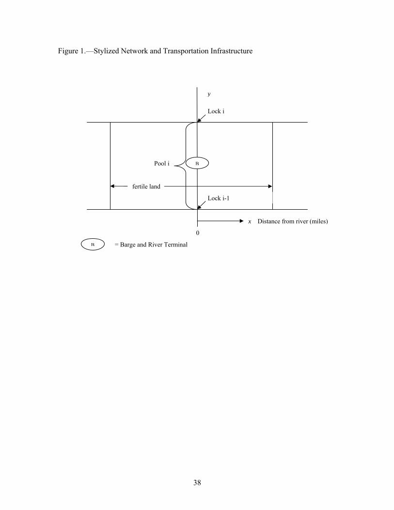
Figure 1.—Stylized Network and Transportation Infrastructure

y

Lock i

Lock i-1

fertile land

Pool i B

x Distance from river (miles)

0

= Barge and River Terminal B

38

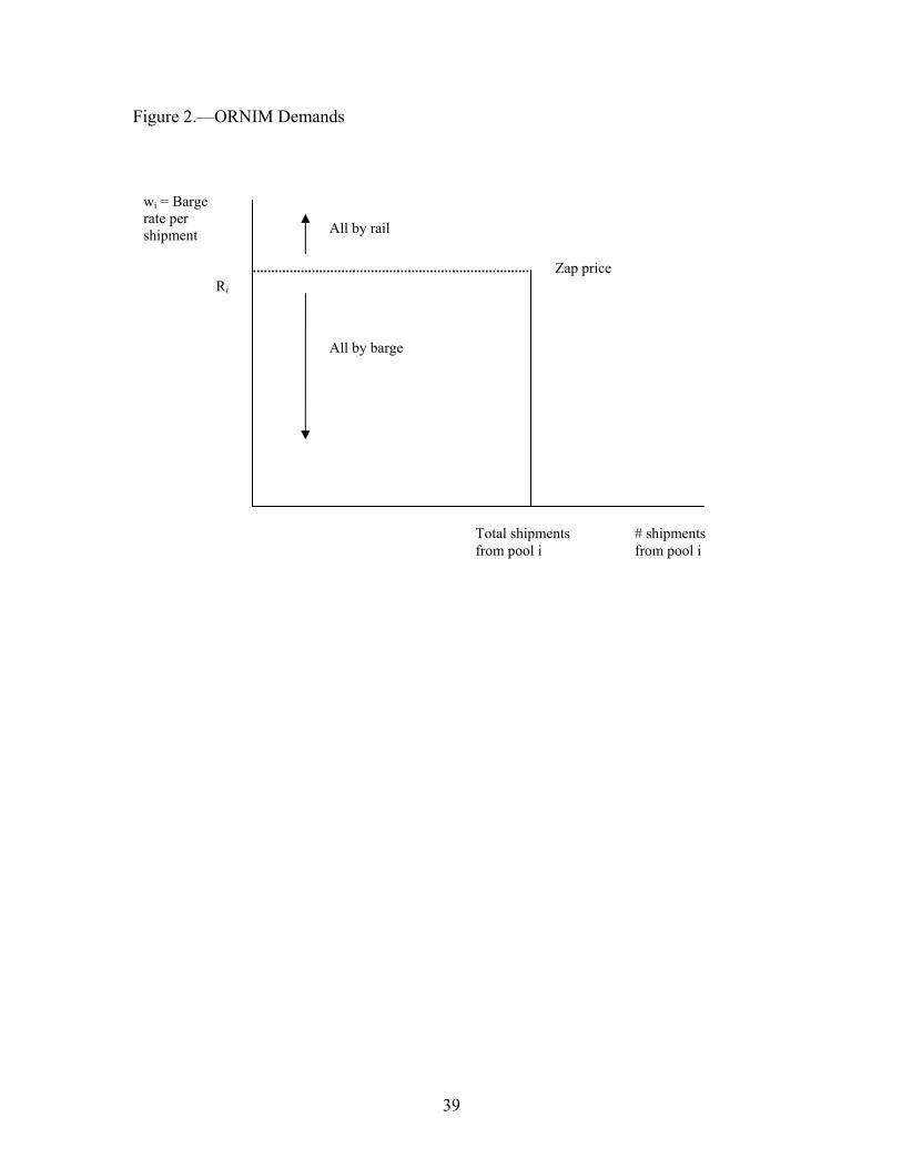
Figure 2.—ORNIM Demands

wi = Barge rate per

All by rail shipment

Zap price Ri

All by barge

Total shipments # shipments from pool i from pool i

39

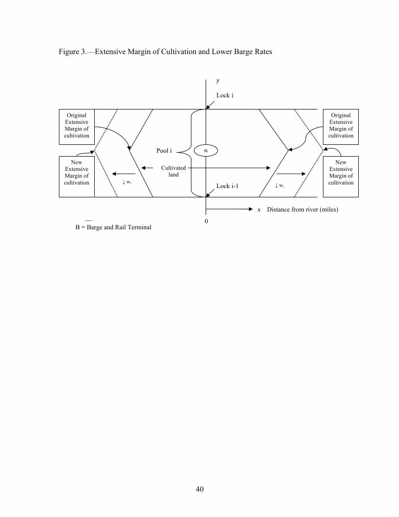
Figure 3.—Extensive Margin of Cultivation and Lower Barge Rates

y Lock i

Lock i-1

Cultivated land

Pool i B

0

x Distance from river (miles)

New Extensive Margin of cultivation

Original Original Extensive Margin of cultivation

Extensive Margin of cultivation

New Extensive Margin of cultivation ↓ wi ↓ wi

BB = Barge and Rail Terminal

40

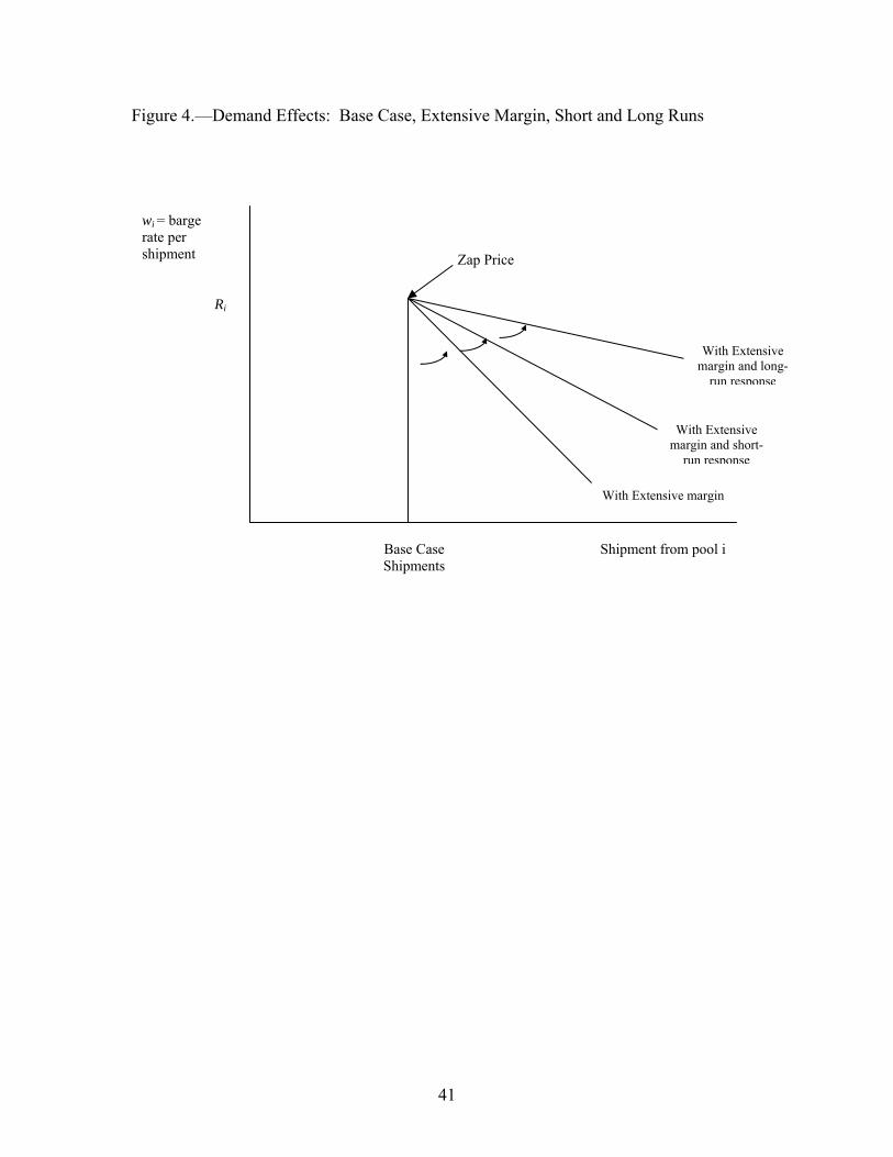
Figure 4.—Demand Effects: Base Case, Extensive Margin, Short and Long Runs

wi = barge rate per shipment

Ri

Zap Price

With Extensive margin and long-

run response

With Extensive margin and short-

run response

With Extensive margin

Base Case Shipment from pool iShipments

41

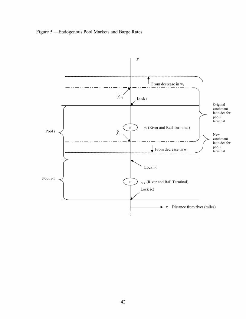
Figure 5.—Endogenous Pool Markets and Barge Rates

Lock i-1

Lock i

Pool i B yi (River and Rail Terminal)

Pool i-1

Lock i-2

Original catchment latitudes for pool i terminal

yi-1 (River and Rail Terminal)

From decrease in wi

From decrease in wi

1ˆiy +

y

ˆiy New catchment latitudes for pool i terminal

B

x Distance from river (miles)

42

0

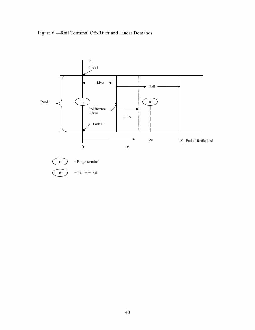
Figure 6.—Rail Terminal Off-River and Linear Demands

Lock i-1

y

Lock i

Pool i B

0 1x End of fertile land

x

xR

IndifferenceLocus

River Rail

R

↓ in wi

= Barge terminal B

= Rail terminal R

43

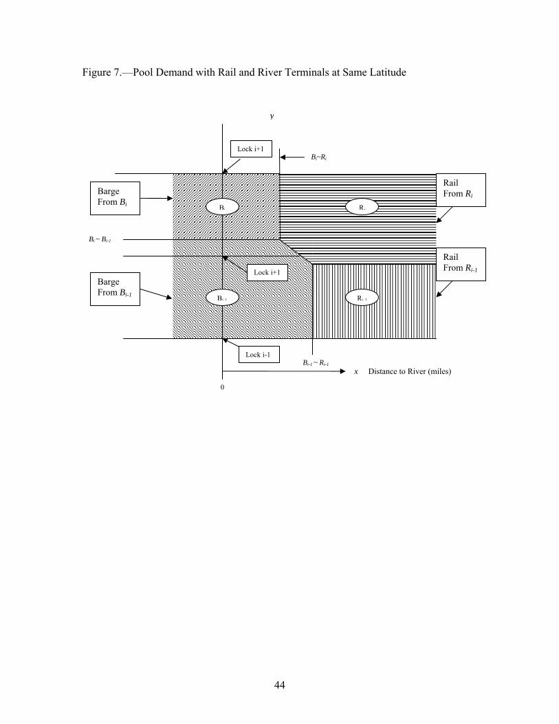
Figure 7.—Pool Demand with Rail and River Terminals at Same Latitude

y

Lock i+1

Barge From Bi

Barge From Bi-1

Rail From Ri

Rail From Ri-1

Lock i-1 Bi-1 ~ Ri-1

Bi~Ri

Bi ~ Bi-1

0

Bi Ri

Lock i+1

Bi 1 Ri 1

x Distance to River (miles)

44

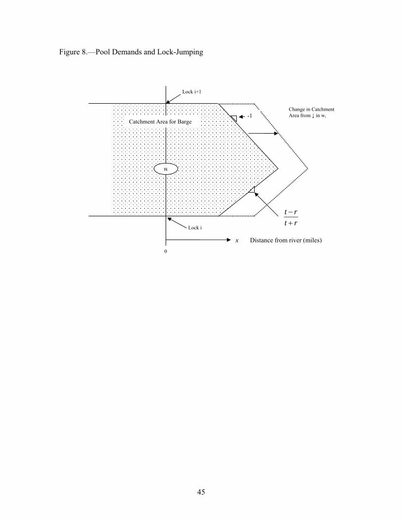
Figure 8.—Pool Demands and Lock-Jumping

Lock i+1

B

Lock i

-1

t rt r−+

Change in Catchment Area from ↓ in wi

Catchment Area for Barge

x Distance from river (miles) 0

45

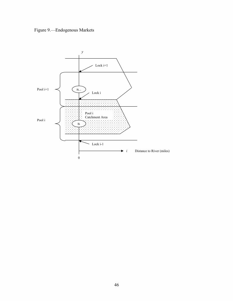
Figure 9.—Endogenous Markets

y

Lock i+1

Lock i-1

Bi+1Pool i+1 Lock i

Pool i Catchment Area

Pool i Bi

i Distance to River (miles)

0

46

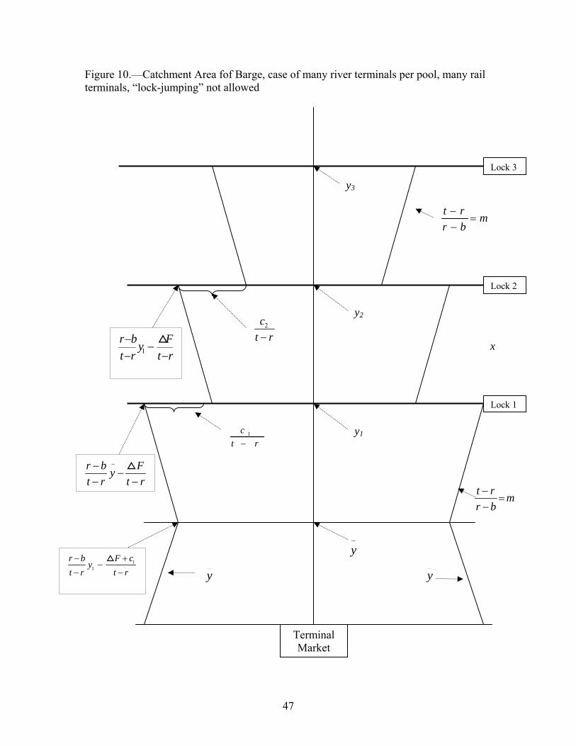
Figure 10.—Catchment Area fof Barge, case of many river terminals per pool, many rail terminals, “lock-jumping” not allowed

~y

x

Lock 3

Lock 1

y1

y3

t r mr b−

=−

y2

t r mr b−

=−

2ct r−

1ct r−

1r b Fyt r t r−

−− −

Lock 2

~r b Fyt r t r−

−− −

_

y _

y 1

1

F cr by

t r t r+−

−− −

Terminal Market

47

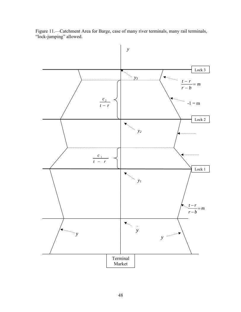
Figure 11.—Catchment Area for Barge, case of many river terminals, many rail terminals, “lock-jumping” allowed.

~y

Lock 1

y1

y3

y2

t r mr b−

=−

Lock 3

2ct r−

1ct r−

Lock 2

t r mr b−

=−

y

-1 = m

_

y _

y

Terminal Market

48

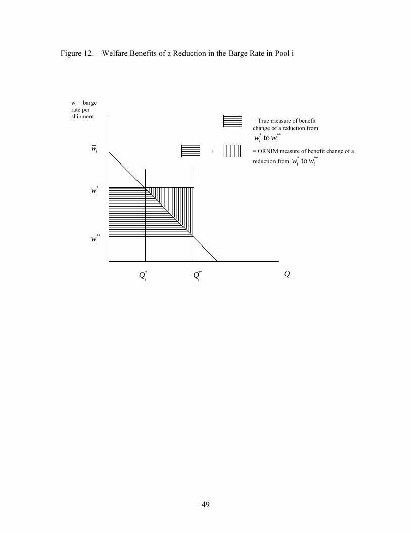
Figure 12.—Welfare Benefits of a Reduction in the Barge Rate in Pool i

iw

*i

w

**i

w

*i

Q **i

Q Q

= ORNIM measure of benefit change of a

reduction from * *toi iw w *+

= True measure of benefit change of a reduction from

* *toi iw w *

wi = barge rate per shipment

49