Market Power in Transportation: Spatial

Equilibrium under Bertrand Competition ∗

Simon P. Anderson†and Wesley W. Wilson‡

June 2014, revised September 2014

Abstract

We examine spatial competition along a waterway when shippers are

distributed over space. Competition is between barge and rail compa-

nies and among barge companies. Equilibrium prices are derived for

two variations: oligopolistic rivalry between barge and rail operators, and

oligopolistic rivalry among barge operators with terminals located at dif-

ferent points on the waterway. In the first variant, each mode has an

advantage over some shippers and transporters’ overprice cost advantages

(price differences are too small in equilibrium). The second variant de-

livers a “chain-linked” system of markets, whereby cost changes in one

market are passed through equilibrium prices to other markets. Barge

operators with cost advantages parlay these into market size advantages.

∗We would like to thank the Navigation Economic Technologies (NETS) program for sup-

port. NETS was an Institute for Water Resources research program in the Army Corps of

Engineers to enhance its mission in assessing waterway investments. This research was one

of the projects: others can be found on www.corpsnets.us. We thank two anonymous referees

and Andre de Palma for their constructive and clarifying comments.†Department of Economics, University of Virginia. Anderson would like to acknowledge

his debt to Richard Arnott for both supervising his PhD thesis, and for Richard’s continual

insights and inspiration into spatial and urban economics.‡Department of Economics, University of Oregon.

1 Introduction

Suppliers of transportation have facilities to serve demanders located over geo-

graphic space, and spatial differences give rise to market power. We develop a

model of equilibrium prices that explicitly recognizes the spatial heterogeneity

of suppliers and demanders of transportation. The suppliers of transportation

services offer rates from different locations to the final market(s). The deman-

ders (or shippers) also are located at different points in space and as such have

heterogeneous preferences across suppliers: ceteris paribus, a closer supplier

is preferred. This latter feature imbues the suppliers with market power over

those shippers located close by. We consider oligopolistic rivalry first between

barge and rail and then among barge companies with spatial location differ-

ences. We examine the implications of spatial heterogeneity and market power

on the effects of transportation infrastructure investment.

Two main variants are considered in order to address two different aspects of

market power in spatially extenuated markets, namely, competition with alter-

native modes and competition with other operators in the same mode. We first

set out the competitive version of the two variants, assuming that modes are

priced at marginal cost. We then address market power in the transport sector

by assuming that transport rates are set in a non-cooperative equilibrium by op-

erators that have market power due to spatial proximity to some shippers. Even

though competition is in prices (the ”Bertrand” assumption), equilibrium prices

are not set at own marginal cost or rival marginal cost (this is in contrast with

spatially discriminatory Bertrand price equilibrium, as analyzed in Anderson

and Wilson, 2008). The reason is that transport operators have some market

power by dint of their closer location for some of the shippers, and they also

are assumed to set a single rate for all shippers served (the no discrimination

assumption).

1

In the first variant of the model, shippers face a mode choice of whether to

ship by rail or river, and both modes are operated under market power. We

find that whichever mode is cheaper (in terms of fundamental cost) is priced

lower to shippers, and so attract more users. However, it will also carry a higher

mark-up. This latter propensity of operators to overprice (resting on the laurels

of a cost advantage) entails a market failure in the allocation of shippers to

modes. Specifically, the fundamentally cheaper mode is actually under-utilized

in equilibrium.1 As we demonstrate, the social value of cost reductions for a

mode e.g., barge exceeds the price reduction measured over shippers, but still

falls short of that which would be realized if both rail and barge markets were

competitive. Thus, only a portion of the cost reduction is passed on to shippers.

The second variant of the model is complementary to the first. Shippers

can choose the transport provider to choose within a given mode (e.g., which

barge operator). Competition by barge operators then gives rise to a market

structure in which markets are vertically stacked.2 Barge operators compete

with their nearest neighbors upstream and downstream. Their interactions lead

to an equilibrium in which all markets are “chain-linked” as each neighboring

market is affected by its neighbors.

The primary purpose of the paper is to introduce a model of imperfect

competition among modes of transportation operating over a network. In the

model, firms compete for demanders located over space and are supplied by both

rail and barge. This framework is central to assessing the benefits and costs of

infrastructure investments such as locks. Currently, waterway policy-makers

use a single-mode competitive model to judge benefits. Yet, there are a number

of studies (e.g., MacDonald, 1987, Anderson and Wilson, 2008) which point to

1Similar results were derived by Anderson and de Palma (2001) in a much different context,

namely a logit demand model where firms differ by the quality of the product offered. To the

best of our knowledge, these results have not been developed in the spatial context.2A somewhat similar spatial demand system is set up for Cournot competition in Anderson

and Wilson (2005).

2

the effects of inter-modal competition on prices. Still others (e.g., Train and

Wilson, 2004, 2008a, 2008b) examine shippers’ choices and find that markets

(i.e., rail and barge) are connected through the demand side. In the present

work, we examine the effects of market power over the network both within a

mode as well as between modes.

Our work is motivated by the need to calculate benefits of waterway invest-

ment by planners in the U.S. but may be applicable in other cases as well. The

U.S. Army Corps of Engineers maintain and manage the U.S. waterway system

(see the map in the Appendix). The inland waterway system has a network of

about 12,000 miles, and handles about 300 billion ton-miles annually (Vachal et

al., 2005). The commodities transported are generally bulk commodities (e.g.,

agricultural, coal, petroleum) and composition varies across rivers - the Upper

Mississippi downstream traffic is dominated by agricultural movements, Ohio

River traffic is dominated by coal, etc.

Demand derives from spatially distributed shippers that make modal deci-

sions which can and do vary over locations. Supply is provided by truck, rail

and barge. While there are a large number of trucking firms, there are only

seven major railroads with whom barge companies compete with for longer

haul distances. There are large numbers of barge companies that provide ser-

vice. However, the number of water carriers varies across rivers and within

rivers. For example, supply on the Columbia-Snake River is dominated by a

single carrier which competes vigorously with railroads (which fits well with the

model presented in Section 3).

We also consider barge-barge competition. Indeed, while the number of

barge companies that operate in the U.S. is seemingly large (Vachal et al.,

2005), they tend to be somewhat specialized in location and service. Using data

described in Wilson (2006) that pertain to the Upper Mississippi, we are able

to shed more light. Those data consist of movements through the 29 locks of

3

the Upper Mississippi waterway for the year 2000. There are 83 companies that

haul commodities southbound. For overall traffic (all locks), the market shares

are generally quite small but can be as large as 24 percent. In terms of standard

market structure measures, the four firm concentration ratio for traffic passing

through the locks is about 66 percent, with a Herfindahl index of 1253. At the

lock level, a more narrow market definition, the number of carriers ranges from

two to sixty-seven at the 29 locks on the Mississippi waterway. The four firm

concentration level ranges from 60 percent to 100 percent, and the Herfindahl

ranges from 1189 to 9851 with an average value of 2179. It is clear that, based

on these figures, the level of competition varies widely along the river. In some

locations, the number of carriers is quite small, while in other locations the

number of carriers is larger, but the overall indicators of concentration does

point to the potential for barge-barge competition addressed in Section 4.

The next section sets out the basic model. Section 3 analyzes the first

variant (rail vs. barge), while Section 4 gives the set-up and results for the

second variant (intra-barge competition). Section 5 offers some conclusions.

2 The benchmark template for barge-rail and

barge-barge rivalry

The geography of the benchmark model is shown in Figure 1. There is a river

running from the North to the South along the -axis (i.e., = 0). Assume

that the shippers are located with uniform density over a region of width

contiguous to the river (this can be thought of as a river valley, say, of fertile

land). In the first variant, there is also a parallel railway line at = 0

(the other side of the shippers’ locations). There are river terminals at latitudes

, = 1 , indexed so that a higher value of indicates a location further

North. We denote by the cost of shipping a unit of the commodity from

4

latitude by river (i.e., by barge) all the way to the final transshipment point

(in this case, the southern-most point).3 Per unit shipping costs rise with the

distance shipped, so that as . These costs denote the actual costs

faced by the transport operators. The latter set rates above costs to shippers

since the operators have market power.4

INSERT FIGURE 1. Economic Geography for Barge-Rail Competition

Likewise, in the first variant of the model when we focus on competition

between barge and rail, the cost of shipping a unit of the commodity from

latitude by rail to the final transshipment point is , with with

. It is assumed that each river terminal has a parallel rail terminal (i.e., at

the same latitude as the river terminal).5 We assume that these locations are

exogenous. We further assume that so that rail transportation is more

costly. Since the rail terminal may be closer to some shippers’ locations than

the river terminal, this does not preclude rail being used by shippers. Moreover,

shipping prices are determined by barge operators and by rail companies, and,

in equilibrium, these prices reflect a trade-off between volume transported and

mark-up earned. The first objective is to determine how these prices reflect

competitive conditions and costs.

To focus on rail-barge rivalry, we assume away rivalry among barge operators

(which is the focus of the next Section.) This we do by assuming that the

latitudinal boundary between neighboring barge operators is fixed at , with

∈ ( −1). This assumption prevents competition across the latitudinal3Much of our work is motivated by agricultural shipments on the Mississippi to New Orleans

for export. Ninety percent of corn shipments that originate upstream terminate in the New

Orleans area (Boyer and Wilson, 2005).4Thus, we refer to the prices paid by shippers as rates (even though these are the costs

paid by the shippers), and we reserve the term ”costs” for the fundamental costs.5This we do in order to bring out the basic tensions of competitive rivalry in the clearest

manner. The qualitative results should not change if the rail terminals are at different lat-

itudes, though the demand expressions and the equilibrium analysis would be substantially

more cumbersome.

5

boundary and allows it only between rail and barge within a given band (or

stripe) of latitudes.6

The commodity is trucked from the hinterland to either a river terminal

or a rail terminal, at rate per unit per mile. As noted above, we initially

assume that shippers must ship to the closer latitude (this will be addressed

separately as the main focus of attention in the second variant of the model).

Truck transportation follows the block metric (distance between two points is

measured as the sum of their vertical and horizontal displacements) and so,

for given rates charged for rail and barge transportation, the hinterland will

be split into blocks corresponding to demand regions: blocks nearest the river

will use barge transportation. A further rationale for analyzing this set-up is

that it corresponds most closely to the basic Samuelson-Takayama-Judge (STJ)

assumption that catchment areas are fixed, but at the same time it allows for

competition by transportation mode within each ”region” for shippers.7

Figure 1 is drawn for the case of Barge-Rail competition of the next Section,

but the only major change for the Barge-Barge competition model of Section

4 is that the railway is not present and competition is between neighboring

barge terminals instead. For the Barge-Rail competition case, as illustrated,

competition is between barge and rail for each given strip of territory between

given latitudes: all shippers between and +1 must choose between the river

terminal at latitude (and longitude = 0) and the rail terminal at latitude

(and longitude = ).

Finding equilibrium prices within each region requires the determination of

transporters’ profits as function of the prices charged by themselves and their

6For example, could be the location of a lock, and we invoke a ”no-lock-jumping”

assumption. Alternatively, we could use the market boundaries defined from perfectly com-

petitive conditions between barge operators. Then the boundary, as derived below, is given

as =+1−

2+

+1+2

.7We consider this connection in greater detail in related work (Anderson and Wilson, 2004,

2007).

6

rivals. This means that we must first find transportation demand as a function

of prices. The next two sections pick up at this point for their respective models.

3 Barge-rail rivalry

In this variant, we concentrate on competition between modes, leaving intra-

mode competition for the next variant. Accordingly, we assume that the latitude

decision is fixed exogenously: for concreteness, assume that all shippers between

and +1 choose either to ship from the river or rail terminal at latitude

(so the only choice shippers must make is between river and rail), with ∈( +1). Under these assumptions, the market at any latitude is determined

by the location of the shipper indifferent between the relevant rail and river

options.

Let be the price charged at latitude for rail transport (per unit)8 and

be the corresponding price for river transport. Shipping by river from longitude

incurs a price of + || (ignoring the North-South trucking cost to therelevant latitude, latitude , since this is common to both options).

9 Shipping

by rail (again net of the trucking cost to latitude ) incurs a price of + | − |from longitude .

When there is perfect competition at each mode, the transport rates are

for rail and for barge. The market split point is then given as the solution to

+ || = + | − |, i.e.,

=

2+

−

2 (1)

8Wilson (1996) considers rail pricing in the context of differentiated modes. In his model,

the railroad chooses whether it wants the traffic and then how much can they charge. This

latter is the maximum of the monopoly price or the price at which the railroad loses the traffic

to another mode.9That is, total trucking cost if the shipment is later taken by barge is || + | − |;

if the shipment is later taken by rail, the total trucking cost is |− | + | − |. Sincethe term | − | is common, it may be ignored in determining the choice of mode for thefinal segment. This means that the market boundaries between barge and rail are vertical

(North-South): the property follows from the block metric for transportation.

7

The situation is illustrated in Figure 2. The sloped lines represent the full

price paid as a function of lateral distance from the terminals for barge and

rail, incorporating the lateral trucking costs, giving the slopes at rate . As

illustrated, the barge rate is lower than the rail rate, so that the market split

(at , East of ) induces a larger market for barge than rail.

INSERT FIGURE 2. Barge-Rail Market Division (longitudinal split).

As should be clear from Figure 2, the relevant portion of Figure 1 is a

horizontal line between rail and barge ports at latitude . That is, the North-

South components of Figure 1 are irrelevant in this simple setup. The market

split relation in (1) indicates several properties. First, if barge and rail rates

are equal, the market splits equally between modes. All shippers closer to the

river ship from there, and all shippers closer to the rail terminal ship by rail.

The market demand for barge decreases in its own price, and rises in the rival

operator’s price, so the two modes are substitutes for shippers. The rate of

switch-over from one mode to another (the rate at which the marginal shipper

transfers economic allegiance) is inversely proportional to the truck rate (the

switch-over rate is 1/2t per dollar price difference) Thus, the higher the truck

rate, the less responsive are shippers to switching in response to lower barge

or rail rates. This natural property follows because as higher rates imply the

share of barge and rail costs relative to overall costs decline, and this reduction

reduces rate responsiveness.

The same properties hold when rates are set with market power, although

then the rates are determined by the transport operators. These rates depend

upon the basic costs, and . For given rates, the market splits in region at

=

2+

−

2 (2)

This differs from (1) only insofar as the competitive rates, and , are now

8

determined by transport operators as and (and so the basic picture in

Figure 2 now holds with and in lieu of and .)

The basic market power analysis is based on an asymmetric version of

Hotelling’s (1929) model.10 In addition to considering the asymmetries, the

current version is also distinctive for the comparison of stacked markets (and

the variant in the next Section is distinctive for the analysis of rivalry between

such stacked markets).

Given the demands, as embodied in (2), we can now turn to profits. For a

barge operator operating from a river terminal at latitude , profits are then

given by:

=¡ −

¢ (3)

which is the product of the mark-up and the demand. The barge operator thus

faces a trade-off: the larger the mark-up, the lower the volume of sales, and vice

versa. Similarly, profits for rail (operating from a river terminal at latitude )

are given by:

= ( − ) ( − ) (4)

The first-order condition for determining the barge rate are then

= −

¡ −

¢2

= 0 (5)

The first term is the extra revenue on the existing customer base for a $1 in-

crease. The second one is the lost revenue (the mark-up) on the lost consumer

base (which is lost at rate 12). The analogous first-order condition for the rail

operator is:

= ( − )− ( − )

2= 0 (6)

10Hotelling’s simple framework remains an enduring one that has attracted many re-

searchers. Hotelling’s approach furnished a canonical model not just for studying equilibrium

locations, but also for simple product differentiation, political competition, marketing deci-

sions, and a host of other applications. Some of these are detailed in Anderson (2005), and

reviews of models in Hotelling’s vein are found in Anderson, de Palma, and Thisse (1992,

Chapter 8), Archibald, Eaton, and Lipsey (1989), Enke (1951), and Gabszewicz and Thisse

(1992).

9

Note that the second-order conditions clearly hold (the profit functions are con-

cave quadratic functions). The first-order conditions define the reaction func-

tions for the operators. These reaction functions, and the associated equilibrium

at their intersection, are illustrated in Figure 3. The Figure embodies the as-

sumption that exceeds : the fundamental cost per unit shipped is higher

for rail than barge.

INSERT FIGURE 3. Reaction Functions and Equilibrium for Barge-Rail

Formulation

Each reaction function embodies the property that a $1 rise in its rival’s

transport rate will raise its own optimal (best reply) rate by 50 cents. Hence

the equilibrium is unique and stable. Reaction functions slope up and so the

transport rates are ”strategic complements” (they move together).

The explicit equilibrium solution can be derived from the first-order condi-

tions. We have from (5) and (6) above that =(−)2

and ( − ) =(−)2

.

These are respectively rewritten as

= 2 + (7)

and

= 2 ( − ) + (8)

Then recall from (2) that =2+ −

2which enables us to solve for from

the relations (7) and (8) above as:11

=

2+

−

6(9)

in equilibrium.12 Note that the market splits at the mid-point under symmetry

of fundamental costs. Note too that the solution is independent of monetary

11Since =2+

2(−2)+−2

or 3 =32+

−2

and hence (9) follows directly.12If

2+

−6

≥ , then the whole market is served by the barge operator. Equivalently,

the condition is written as ≥ + 3.

10

measures and depends on the ratio of transport rates: if all transportation

prices doubled, the solution does not change. Market power cushions the im-

pact of fundamental cost changes: the equilibrium change is at rate 1/6t while

the perfectly competitive counterpart is at rate 1/2t per dollar change in the

fundamental costs.

We can now back out the equilibrium transport rates. In particular, since

= 2 + then = ³ + −

3

´+ or

= +1

3

¡ + 2

¢ (10)

This shows some interesting absorption properties. First, each $3 rise in own

shipping cost feeds through into a rise in equilibrium shipping rate charged of

$2. The transport provider absorbs the other $1 itself for fear of giving up too

much market to its rival. Likewise, an increase of $3 in the rival’s cost feeds

through into an own price increase of $1. The explanation follows from strategic

complementarity (the property that the reaction functions slope up: see Figure

3 above).

Similarly, = 2³ −

2− −

6

´+ , or

= +2 +

3 (11)

In particular, it can readily be seen that the operator with the lower cost of

transport (i.e., whether or is lower) also has the lower price. Nonetheless,

its mark-up is higher, it gets a greater fraction of the market, and its profit is

also higher. These important properties are readily proved. The intuition is as

follows. Suppose that barge transportation is less costly than rail. The barge

operators use this advantage to increase mark-ups, but not so much as to reduce

their market areas. Put another way, barge operators use their advantage to

both enjoy higher mark-ups and larger markets; meaning that the prices they

charge are still below the rail operators’ prices.

11

These properties are reflected in smaller market areas than is optimal for

barge (and larger market areas than is optimal for rail).13 To see this, note that

the socially optimal allocation involves both modes priced at cost, leading to an

optimal allocation of

=

2+

−

2 (12)

Then, as long as , we have . This follows since =

2+ −

6by

(9).

We can next find the implications for prices as a function of distance. Sup-

pose, for illustration, that the fundamental price for both rail and barge rise with

distance, and that the rail price is proportional to the barge one, with constant

of proportionality 1 (so that rail costs are higher than barge costs). Then

we find that the rail price charged always exceeds the barge price, although the

barge mark-up is higher. Furthermore, the barge catchment area is larger the

further away from the terminal market. That is, barge serves a larger fraction

of the shippers the closer to the source of the river. To see this latter property,

it suffices to write the equilibrium market share relation as (using (9)):

=

2+

−

6=

2+(− 1)

6

This is clearly increasing in , and hence in distance.14 However, the optimal

allocation between barge and rail is

=

2+(− 1)

2

This means that market power in the transportation sector induces the distor-

tion that the market area for barge is too small (since the mark-up is too big).

13Recall though we have assumed that both the barge provider and the railway have equal

market power. This assumption drives the result. If, instead, we assumed that barge operators

priced perfectly competitively, rail markets would be too small (and barge markets too large),

but the ”fault” would lie squarely with the rail operator for pricing too high. In an earlier

paper, Anderson and Wilson (2008), we covered just such a case and derived this result.14It is apparent from the formula that the whole market is served by barge as long as

(−1)6

≥ 2.

12

Since barge has been assumed to be cheaper, and market power has been taken

as equally strong on both sides of the market, the barge sector overprices its

advantage. We should note that this analysis has simply assumed that market

power is equally strong in the barge market as in the rail market, with the

purpose of theoretically deriving the efficiency implications of market power. If,

instead, the barge market is taken as perfectly competitive while the rail market

has the market power, the rail market is over-priced relative to barge and it is

the rail market that is too small.

We can also derive the implications of a transportation cost reduction, for

concreteness, a decrease in the cost of barge shipping. This is manifest as a

reduction in . This change induces a reduction in the price charged for barge

transportation that improves the well-being of shippers using barge. Since the

price reduction is less than the cost reduction, the barge operators are better

off, enjoying greater profits. However, rail operators are worse off because they

face tough competition. Rail operators’ profits fall for two reasons. First, they

face lower prices from the rival mode, inducing lower profits, and second, they

have smaller markets served. Shippers in the rail segment also gain from the

cost improvement in the barge sector. This is because they pay lower prices

for rail, even though there is no cost reduction there. The tougher competition

induces lower prices for shippers. Hence, the social value of the improvement

exceeds the price reduction as measured over the barge shippers. Nonetheless,

the social value falls short of what it would be if there were perfect competition.

This is because the allocation remains distorted: the cost reduction is only par-

tially passed on to the shippers, and hence only partially matched by the rail

operators.

13

3.1 Introducing time costs

In the model so far, shipper choices are driven by prices alone. Time enters

only through the costs of traveling through a lock. There is, of course, a history

of research that indicates shippers care not only about rates, but also quality

of service, which includes transit times and reliability (see, for example, Train

and Wilson, 2004, 2008a, 2008b). Indeed, it is commonly recognized that barge

rates are lower than rail which are lower than truck. While costs are lower in

the same direction, the service by barge is slower than rail which is slower than

truck.

We now show how the basic model is readily amended to allow shipper

choices to also depend on differential time costs across transport modes. The

basic insights and take-aways still hold with appropriate reinterpretation of

parameters.

To see this, we now suppose that time costs for barge and rail from latitude

take monetary equivalents and respectively. Notice that these could

vary across the shipping season (just as the base opportunity costs and can

vary too), so that equilibrium rates will accordingly vary as a consequence.

The ”full prices” to shippers (denoted by superscripts, and exclusive of the

trucking cost to the relevant terminal) from barge and rail comprise the sum of

money and time costs. Thus full prices paid are = + and

= +

respectively. The market split condition (2) is as before except now with full

prices in place of the former time-cost exclusive ones. Likewise, we can write

the operators’ profit margins as¡ −

¢=³ −

¡ +

¢´and likewise for

rail. The duopoly game for choosing rates ( and ) is strategically equivalent

to choosing them full prices. Therefore the profit functions we had before, (3)

and (4), take the same form and have the same solutions. The difference is that

the solutions corresponding to and are now in terms of full prices, and costs are

14

now ”full” costs, i.e., the sum of costs to shippers and the monetized time costs

borne by shippers. That is, the solution is (using (10) and (11))

= +

( + ) + 2¡ +

¢3

(13)

and

= +

2 ( + ) +¡ +

¢3

(14)

Rates received by transport operators are found by subtracting the time costs.

That is, we now have

= + + 2 + −

3

and

= +2 + + −

3

Hence these rates pass on transport costs in the same manner that they did in

the simpler incarnation (which is seen as the special case = ). The rates

also now embody time cost advantages, absorbing a fraction (a third) of own

cost, and charging the same fraction for the rival mode’s time cost. Thus, as

noted above, if barge has a higher time cost, then this feeds through into a

higher rail rate and a lower barge rate.

4 Barge-barge competition

We now turn to the case of barge-barge competition. For this purpose, we

assume that railroads do not exist, which allows us to focus directly on ri-

valry amongst barge carriers. Assume again that the shippers are located with

uniform density over a region of width contiguous to the river.15 The new

economic geography is depicted in Figure 4 for the case of perfectly competitive

operators. The difference with Figure 1 is that there is no competition from rail

15More complex versions of the model would have reservation prices that would bind for

some shippers, etc. See e.g., Bockem (1994) for an analysis with symmetric firms.

15

and the market boundaries are endogenously determined. We also explicitly

allow for shippers at the most Southerly locations to ship directly by truck to

the terminal market, and for shippers at the most Northerly locations to ship

to an alternative market, as described below.

INSERT FIGURE 4. Economic Geography for Barge-Barge Model.

First, suppose that barge operators were to price at marginal cost (this is

the perfect competition back-cloth benchmark). Then is the price of barge

transportation from to the final market. Neighboring barge markets are

separated at the latitude as determined by

−1 + [ − −1] = + [ − ] = 1 (15)

where the left hand side is the cost for a riverside shipper at to ship from the

next river terminal to the South, at −1, and the right hand side is the cost for

a riverside shipper at to ship from the next river terminal to the North, at

. Hence, is determined as

= − −12

+ + −1

2

Shippers at the lowest latitudes will just ship by truck to the final market.

The farthest south barge operator therefore faces competition from truck for the

haul. The southern latitudinal margin of competition for its market, 1, is there-

fore determined endogenously by its shipping cost, 1, according to the indiffer-

ence condition for the shippers along the boundary, namely 1 = (1 − 1)+1,

where the LHS is the north-south cost of trucking from the boundary, and the

RHS is the cost of trucking north to the barge terminal and then taking barge

down the river. Notice that our assumption of the simple block metric for truck

transport is instrumental in delivering a clean lateral market boundary. Fur-

thermore, notice that the equation for 1 is commensurate with the ones for the

16

other margins of competition by setting 0 = 0 (so there is no market power

held over shippers in the truck market), so that

1 =1

2+

1

2

At the other end, for symmetry with this treatment, suppose that the ter-

minal the farthest to the North ships to an alternative final market (the Pacific

Northwest, say). Assume that this rate is set perfectly competitively, at +1.

Then the furthest north market boundary is given as

+1 =+1 −

2+

+1 +

2

The situation is quite similar under rivalrous barge operators exercising spa-

tial market power. Then neighboring barge markets are separated at the latitude

as determined by

−1 + [ − −1] = + [ − ]

Again, the left hand side is the cost for a riverside shipper at to ship from

the next river terminal South (at −1); the right hand side is the cost for a

riverside shipper at to ship from the next river terminal North (at ). Now

is

= − −12

+ + −1

2

For the lowest market (the one farthest to the South), as explained above,

0 = 0 and

1 =1

2+

1

2

Likewise, given +1, the furthest North market boundary is

+1 =+1 −

2+

+1 +

2

17

We can now write out the profits for a barge operator operating from a river

terminal at latitude , = 1 . These are then given by16:

=¡ −

¢(+1 − ) (16)

which is the product of the mark-up and the demand. The barge operator thus

faces a trade-off: the larger the mark-up, the lower the volume of sales, and vice

versa. The first-order condition for determining the barge rate are then

= (+1 − )−

¡ −

¢4

= 0 (17)

The first term is the extra revenue on the existing customer base for a $1 in-

crease. The second is the value of lost shippers: they switch at rate 1/4t count-

ing the two sides at which they switch. The formulation already embodies the

property that large markets are associated to high mark-ups.

We can now solve for the market boundaries to yieldµ+1 −

2+

+1 +

2− − −1

2− + −1

2

¶=

¡ −

¢4

Simplifying,

5 − 2 (+1 + −1) = 2 (+1 − −1) +

Divide through by 5 and then denote the Left-Hand-Side by =2(+1−−1)+

5,

= 1 . Also, denote the constant coefficient that comes from the structure

of the problem as = 25, in order to see clearly the structure. Then these

equations may be written

− (+1 + −1) =, = 1

Although each barge operator competes directly only with its nearest neighbors

upstream and downstream, markets are chain-linked through their interaction.

Then we can write the system of stacked demands in matrix form as

16We neglect here the factor of proportionality that represents the width of the market, ,

and the density of shippers. The product of these two factors has effectively been normalized.

18

⎡⎢⎢⎢⎢⎢⎢⎢⎢⎢⎢⎣

1 0 0 0 0 0 0 0

− 1 − 0 0 0 0 0

0 − 1 − 0 0 0 0

0 − 1 − 0 0

0 0 0 − 1 − 0

0 0 0 0 0 − 1 −0 0 0 0 0 0 0 1

⎤⎥⎥⎥⎥⎥⎥⎥⎥⎥⎥⎦

⎡⎢⎢⎢⎢⎢⎢⎢⎢⎢⎢⎣

012

+1

⎤⎥⎥⎥⎥⎥⎥⎥⎥⎥⎥⎦=

⎡⎢⎢⎢⎢⎢⎢⎢⎢⎢⎢⎣

0

1

2

+1

⎤⎥⎥⎥⎥⎥⎥⎥⎥⎥⎥⎦

It is understood here that 0 = 0 and +1 = +1: these equations repre-

sent the exogenous market prices at the extremes.

The matrix has an interesting structure, and some properties can be derived

from inverting it. For = 2, the inverse is (setting 2 = 1− 2 = 2125):

⎡⎢⎢⎢⎣1 0 0 02

12

2

2

2

2

2

2

12

2

0 0 0 1

⎤⎥⎥⎥⎦ Hence the solution is

⎡⎢⎢⎣0123

⎤⎥⎥⎦=⎡⎢⎢⎣

01

1−2¡1 + 0 + 2 + 23

¢1

1−2¡2 + 1 + 3 + 20

¢3

⎤⎥⎥⎦Interesting effects from the chain-linking of markets can be seen here. For

instance, a reduction in 3 (e.g., a reduction in costs specific to barges serving

the lower market) reduces both 2 and 1, but it reduces 2 by more than it

reduces 1 through the dampened knock-on effect.

For = 3, we have the inverse as

19

⎡⎢⎢⎢⎢⎢⎣1 0 0 0 0

−33

1−23

3

2

3

3

3

2

3

3

13

3

2

3

3

3

2

3

3

1−23

−33

0 0 0 0 1

⎤⎥⎥⎥⎥⎥⎦,

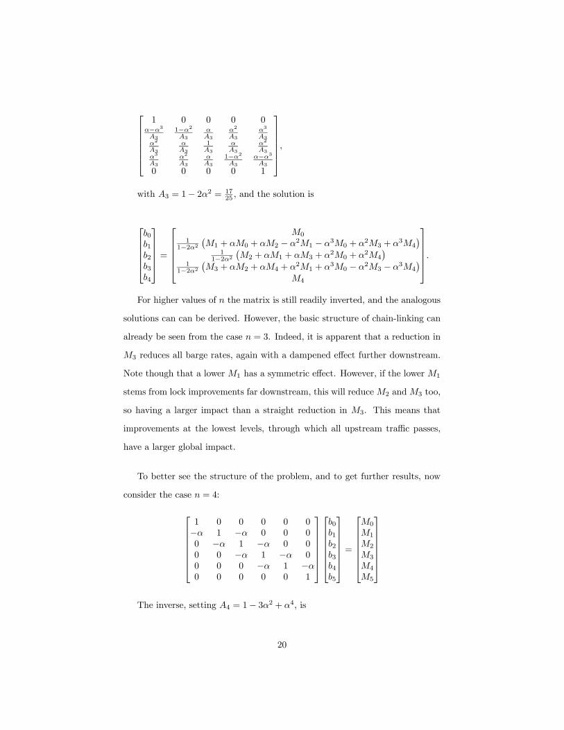
with 3 = 1− 22 = 1725, and the solution is

⎡⎢⎢⎢⎢⎣01234

⎤⎥⎥⎥⎥⎦ =⎡⎢⎢⎢⎢⎣

01

1−22¡1 + 0 + 2 − 21 − 30 + 23 + 34

¢1

1−22¡2 + 1 + 3 + 20 + 24

¢1

1−22¡3 + 2 + 4 + 21 + 30 − 23 − 34

¢4

⎤⎥⎥⎥⎥⎦.

For higher values of the matrix is still readily inverted, and the analogous

solutions can can be derived. However, the basic structure of chain-linking can

already be seen from the case = 3. Indeed, it is apparent that a reduction in

3 reduces all barge rates, again with a dampened effect further downstream.

Note though that a lower 1 has a symmetric effect. However, if the lower 1

stems from lock improvements far downstream, this will reduce2 and3 too,

so having a larger impact than a straight reduction in 3. This means that

improvements at the lowest levels, through which all upstream traffic passes,

have a larger global impact.

To better see the structure of the problem, and to get further results, now

consider the case = 4:

⎡⎢⎢⎢⎢⎢⎢⎣1 0 0 0 0 0

− 1 − 0 0 0

0 − 1 − 0 0

0 0 − 1 − 0

0 0 0 − 1 −0 0 0 0 0 1

⎤⎥⎥⎥⎥⎥⎥⎦

⎡⎢⎢⎢⎢⎢⎢⎣012345

⎤⎥⎥⎥⎥⎥⎥⎦ =⎡⎢⎢⎢⎢⎢⎢⎣0

1

2

3

4

5

⎤⎥⎥⎥⎥⎥⎥⎦The inverse, setting 4 = 1− 32 + 4, is

20

⎡⎢⎢⎢⎢⎢⎢⎢⎣

1 0 0 0 0 0−234

−22+14

−34

2

4

3

4

4

4

2−44

−34

−2+14

4

2

4

3

4

3

4

2

4

4

−2+14

−34

2−44

4

4

3

4

2

4

−34

−22+14

−234

0 0 0 0 0 1

⎤⎥⎥⎥⎥⎥⎥⎥⎦,

and hence we can find the solution for the vector of ’s as⎡⎢⎢⎢⎢⎢⎢⎢⎣

0

2

43 +

3

44 +

4

45 +

14

0

¡− 23¢+ 1

42

¡− 3

¢+ 1

41

¡−22 + 1¢4

3 +2

44 +

3

45 +

14

1

¡− 3

¢+ 1

42

¡−2 + 1¢+ 14

0

¡2 − 4

¢4

2 +2

41 +

3

40 +

14

4

¡− 3

¢+ 1

43

¡−2 + 1¢+ 14

5

¡2 − 4

¢2

42 +

3

41 +

4

40 +

14

3

¡− 3

¢+ 1

45

¡− 23¢+ 1

44

¡−22 + 1¢5

⎤⎥⎥⎥⎥⎥⎥⎥⎦The most striking result from this is what happens when (for example) we

raise 3 and 4 say by $1: this would be like an increase in costs, due to

deteriorating locks say, that is only incurred by the top 2 pools. Nonetheless,

although only 3 and 4 are directly impacted, there is a domino effect down

the line and back up again. The comparative statics are calculated as⎡⎢⎢⎢⎢⎢⎢⎣012345

⎤⎥⎥⎥⎥⎥⎥⎦ =⎡⎢⎢⎢⎢⎢⎢⎢⎣

02

4+ 3

4

4+ 2

414

¡− 3

¢+ 1

4

¡−2 + 1¢14

¡− 3

¢+ 1

4

¡−22 + 1¢0

⎤⎥⎥⎥⎥⎥⎥⎥⎦

Now let us calibrate these numbers using the model’s parameter value =

02, so that −3 (02)2 + 024 + 1 = 08816. This yields⎡⎢⎢⎢⎢⎢⎢⎣012345

⎤⎥⎥⎥⎥⎥⎥⎦ =⎡⎢⎢⎢⎢⎢⎢⎣

0

54× 10−2027

130

126

0

⎤⎥⎥⎥⎥⎥⎥⎦.There is nearly no effect on the price from the farthest away pool, which is

interesting insofar as the chain-link effect dampens quite quickly. However, the

neighbor price (2) has quite a strong rise. The big impact though is on the

21

prices in the top two pools that ship down the river. There the cost pass-on

actually exceeds unity, and by quite a wide margin. Thus, in this system the

cost pass-on in more than 100%, despite the fact that the demand structure is

effectively linear.17

To view this result from the other perspective, suppose instead we envisaged

a situation where the locks were improved and reduced costs to all those up-

stream of the improvements. Not only are shippers downstream better off, but

those upstream are better off by an amount exceeding the actual reduction in

costs per trip. That is, market power of barge operators here is diminished to

such an extent that the social benefits through reduced prices is more than the

cost savings

5 Conclusions

We have examined the consequences of market power in the transportation sec-

tor by means of two different set-ups that highlight first the competition between

barge and rail, and, second, the case of barge and barge competition. In the

first case, assuming equal market power in both sectors, the barge market tends

to over-price the cost advantage which we ascribed to it, rendering the barge

market too small in equilibrium. If, instead, the barge market is competitive

while the rail market has the market power, the rail market will be overpriced

(and the rail market too small).

The second case analyzed suppresses competition with rail and involves only

competition between barge operators with market power. The demand structure

emphasizes the chain-linking of markets, and points to the importance of lock

improvements at the locks (downstream) through which many shipments will

17With linear demands, the monopoly pass-through is 50%. However, with a covered market

(e.g. the classic Hotelling model), raising both costs the same amount causes perfect pass-

through of 100%. The striking result here is that this benchmark is surpassed, even though

the costs have risen for only two firms.

22

pass. A similar chain-linking arises under Cournot competition: Anderson and

Wilson (2005) provide some comparison between this and the current Bertrand

case.

Our work is motivated by the need to assess the benefits of investment in the

waterway infrastructure. The models developed and employed by the policy-

makers are underdeveloped, and this research along with our previous work is

part of a process of improving these assessments. There is, however, consider-

able room for extensions. Specifically, the models are stylized and ought to be

extended to consider two-way traffic, non-uniformities in production, discrete

locations of shippers, and, in the long-run, endogenous locations for rail and

river terminals.

Another important extension would be to allow for congestion not only at

the nodes (i.e., the locks), but also along the links (i.e., the rivers). The bot-

tleneck model of Arnott, de Palma, and Lindsey (1990, 1993) provides useful

modeling background in this regard. Such extensions are centrally important to

empirically implement the model and to evaluate alternative investment strate-

gies such as investment in the node (e.g., increasing the capacity of the locks)

versus investment in the links (e.g., deepening the channels). In addition, for

welfare analyses, there are considerable differences in the emissions by mode,

and the models can be adapted to reflect these differences en route to policy

measures that affect modal splits.

6 References

Anderson, S. P., 2005. Product Differentiation. New Palgrave Dictionary,

Second Edition.

Anderson, S. P., de Palma, A., 2001. Product Diversity in Asymmetric

Oligopoly: is the Quality of Consumer Goods too Low? Journal of Industrial

23

Economics. 49, 113-135.

Anderson, S. P., de Palma, A., Thisse, J. F., 1992. Discrete choice theory of

product differentiation. MIT press.

Anderson, S. P., Wilson, W. W., 2004. Spatial Modeling in Transportation:

Congestion and Mode Choice. Institute for Water Resources Report 04-NETS-

P-06. Available at www.CORPSNETS.US

Anderson, S. P., and Wilson, W. W., 2005. Market Power in Transporta-

tion: Spatial Equilibrium and Welfare under Cournot Competition. Institute for

Water Resources Report 05-NETS-P-04. Available at www.CORPSNETS.US.

Available at www.CORPSNETS.US.

Anderson, S. P., Wilson, W. W., 2007. Spatial Modeling in Transportation:

Infrastructure, Planning and Welfare, in: Plant, J. (Ed.) in Jeremy Plant ed.,

Handbook of Transportation Policy and Administration . CRC Press, Middle-

town, PA. pp. 255-280.

Anderson, S. P., Wilson, W. W., 2008. Spatial Competition, Pricing, and

Market Power in Transportation: A Dominant Firm Model. Journal of Regional

Science. 48, 367-397.

Archibald, G. C., Eaton, B. C., Lipsey, R. G., 1986 Address Models of Value

Theory. In: Stiglitz, J. E., Mathewson, F. G. (Eds.), New Developments in the

Analysis of Market Structure. Cambridge: MIT Press, pp. 3-47.

Arnott, R., de Palma, A. and Lindsey, R. 1990. Economics of a bottleneck.

Journal of Urban Economics, 27, 111-130

Arnott, R., de Palma, A. and Lindsey, R. 1993. A Structural Model of

Peak-Period Congestion: A Traffic Bottleneck with Elastic Demand. American

Economic Review,

83, 161-179.

Berry, S., Hewings, G., Leven, C., 2000. Adequacy of research on upper

Mississippi-Illinois river navigation project. Northwest-Midwest Institute.

24

Bockem, Sabine, 1994. A Generalized Model of Horizontal Product Differ-

entiation. Journal of Industrial Economics, 42, 287-298.

Boyer, K. D., Wilson, W. W. 2005. Estimation of Demands at the Pool

Level. Institute for Water Resources Report 05-NETS-R-03. Available at

www.corpsnets.us

Enke, S., 1951. Equilibrium among spatially separated markets: solution by

electric analogue. Econometrica, 19, 40-47.

Gabszewicz, J. J., Thisse, J. F., 1992. Location. In: Aumann, R. J., Hart,

S. (Eds.), Handbook of game theory with economic applications, Volume 2.

Elsevier.

Hotelling, H., 1929. Stability in Competition. Economic Journal, 39, 41-57.

McDonald, J. M., 1987. Competition and Rail Rates for the Shipment of

Corn, Soybeans, and Wheat. RAND Journal of Economics, 18, 151-163.

Phlips, L., 1983. The Economics of Price Discrimination. Cambridge Uni-

versity Press.

Samuelson, P. A., 1952. Spatial Price Equilibrium and Linear Programming.

American Economic Review, 42, 283-303.

Takayama, T., Judge, G. G., 1964. Equilibrium among spatially separated

markets: a reformulation. Econometrica, 32, 510-524.

Train, K., Wilson, W. W., 2004. Shipper Responses to Changes in Trans-

portation Rates and Times: The Mid-American Grain Study. Institute for Wa-

ter Resources, Army Corps of Engineers Report No. 04-NETS-R-02. Available

at www.CORPSNETS.US

Train, K., Wilson, W. W., 2008a. Transportation Demand and Volume

Sensitivity: A Study of Grain Shippers in the Upper Mississippi River Valley.

Transportation Research Record. 2062, 66-73.

Train, K., Wilson, W. W., 2008b. Estimation on Stated-Preference Experi-

ments Constructed from Revealed-Preference Choices. Transportation Research

25

- Part B. 42, 191-2003

Vachal, Kim, Hough, Jill, and Griffin, Gene, (2005). U.S. Waterways: A

Barge Sector Industrial Organization Analysis. Navigation and Economic Tech-

nologies Report, Institute for Water Resources, Army Corps of Engineers. Avail-

able at http://www.corpsnets.us/docs/IndOrgStudyInlandWaterways/BargeSectorIndusOrg.pdf

Wilson, W. W. 1996. Legislated Market Dominance. Research in Trans-

portation Economics. 4, 33-48.

Wilson, W. W 2006. Vessel, Firm, and Lock Efficiency Measures in Lock

Performance. Transportation Research Record: Journal of the Transportation

Research Board No. 1963, 1-8.

7 Appendix

INSERT HERE: Map of US waterways

26