Spatial Econometric Analysis Using GAUSS

1

Kuan-Pin LinPortland State University

Introduction to Spatial Econometric Analysis

Spatial Data Cross Section Panel Data

Spatial Dependence Spatial Heterogeneity Spatial Autocorrelation

'

i i i i

i i i i

y x

y

x β

'

it i it it

it it i it

y x

y

x β

( , ) 0

( , ) 0

i j

i j

Cov y y

Cov

( , ) 0,

( , ) 0,

it jt

it jt

Cov y y t

Cov t

Spatial Dependence

Least Squares Estimator

1ˆ ( ' ) '

y Xβ ε

β X X X y

( | ) 0

( | )

E

Var

ε X

ε X

21 12 1

221 2 2

21 2

n

n

n n n

Spatial DependenceNonparametric Treatment

Robust Inference Spatial Heteroscedasticity Autocorrelation

Variance-Covariance Matrix1 1ˆ( ) ( ' ) ( ') '( ' )Var E β X X X εε X X X

1 1ˆˆ ˆˆ( ) ( ' ) '[ '] ( ' ) ?

ˆˆ

Var

β X X X εε X X X

ε y Xβ

Spatial DependenceNonparametric Treatment

SHAC Estimator

Kernel Function Normalized Distance

1 1

ˆ ˆˆ ( '), 1, 2,...,

ˆ ˆˆ ( ) ( ' ) ' ( ' )

ij i jkE

i j n

Var

εε

β X X X X X X

( / )

0 1, 1,

ij ij

ij ii ij ji

k K d d

k k k k

/ ,ijd d d bandwidth

Spatial DependenceParametric Representation

Spatial Weights Matrix

Spatial Contiguity Geographical Distance

First Law of Geography: Everything is related to everything else, but near things are more related than distant things.

K-Nearest Neighbors

12 1

21 2

1 2

0

0

0

n

n

n n

w w

w wW

w w

0

1

, 0

1,

ii ij

n

ijj

w w

w i

Spatial DependenceParametric Representation

Characteristics of Spatial Weights Matrix Sparseness Weights Distribution Eigenvalues

Higher-Order of Spatial Weights Matrix W2, W3, … Redundandency Circularity

Spatial Weights MatrixAn Example

3x3 Rook Contiguity List of 9 Observations with 1-st Order Contiguity, #NZ=24

1 2 3

4 5 6

7 8 9

1 2,4

2 1,3,5

3 2,6

4 1,5,7

5 2,4,6,8

6 3,5,9

7 4,8

8 5,7,9

9 6,8

W1st-Order Contiguity (Symmetric)

0 1 0 1 0 0 0 0 0

0 1 0 1 0 0 0 0

0 0 0 1 0 0 0

0 1 0 1 0 0

0 1 0 1 0

0 0 0 1

0 1 0

0 1

0

WAll-Order Contiguity (Symmetric)

0 1 2 1 2 3 2 3 4

0 1 2 1 2 3 2 3

0 3 2 1 4 3 2

0 1 2 1 2 3

0 1 2 1 2

0 3 2 1

0 1 2

0 1

0

An Example of Kernel WeightsK = 1/(ii’ + W)

1 1/2 1/3 1/2 1/3 1/4 1/3 1/4 1/5

1 1/2 1/3 1/2 1/3 1/4 1/3 1/4

1 1/4 1/3 1/2 1/5 1/4 1/3

1 1/2 1/3 1/2 1/3 1/4

1 1/2 1/3 1/2 1/3

1 1/4 1/3 1/2

1 1/2 1/3

1 1/2

1

W1 Non-Symmetric Row-Standardized

0 1/2 0 1/2 0 0 0 0 0

1/3 0 1/3 0 1/3 0 0 0 0

0 1/2 0 0 0 1/2 0 0 0

1/3 0 0 0 1/3 0 1/3 0 0

0 1/4 0 1/4 0 1/4 0 1/4 0

0 0 1/3 0 1/3 0 0 0 1/3

0 0 0 1/2 0 0 0 1/2 0

0 0 0 0 1/3 0 1/3 0 1/3

0 0 0 0 0 1/2 0 1/2 0

W2 Non-Symmetric Row-Standardized

0 0 1/3 0 1/3 0 1/3 0 0

0 0 0 1/3 0 1/3 0 1/3 0

1/3 0 0 0 1/3 0 0 0 1/3

0 1/3 0 0 0 1/3 0 1/3 0

1/4 0 1/4 0 0 0 1/4 0 1/4

0 1/3 0 1/3 0 0 0 1/3 0

1/3 0 0 0 1/3 0 0 0 1/3

0 1/3 0 1/3 0 1/3 0 0 0

0 0 1/3 0 1/3 0 1/3 0 0

U. S. States

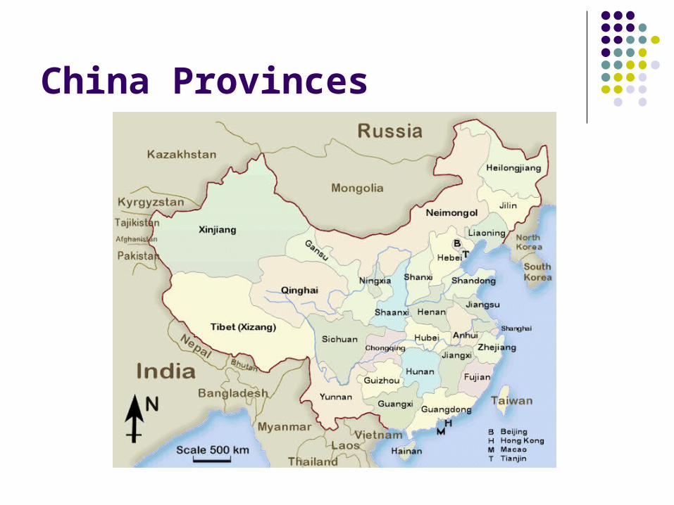
China Provinces

Spatial Lag Variables

Spatial Independent Variables Spatial Dependent Variables Spatial Error Variables

'

1

1,2,...,

n

ij jjw

Wi n

xX

1

1,2,...,

n

ij jjw y

Wi n

y1

1,2,...,

n

ij jjw

Wi n

ε

Spatial Econometric Models

Linear Regression Model with Spatial Variables Spatial Lag Model Spatial Mixed Model Spatial Error Model

Examples

Anselin (1988): Crime Equation Basic Model

(Crime Rate) = + (Family Income) + (Housing Value) +

Spatial Lag Model(Crime Rate) = + (Family Income) + (Housing Value) + W (Crime Rate) +

Spatial Error Model(Crime Rate) = + (Family Income) + (Housing Value) + = W +

Data (anselin.txt, anselin_w.txt)

Examples

China Provincial GDP Output Function Basic Model

ln(GDP) = + ln(L) + ln(K) +

Spatial Mixed Model ln(GDP) = + ln(L) + ln(K) + w W ln(L) + w W ln(K) + W ln(GDP) +

Data (china_gdp.txt, china_l.txt, china_k.txt, china_w.txt)

Examples

Ertur and Kosh (2007): International Technological Interdependence and Spatial Externalities 91 countries, growth convergence in 36 years

(1960-1995) Spatial Lag Solow Growth Model

ln(y(t)) - ln(y(0)) = + ln(y(0)) + ln(s) + ln(n+g+) + W ln(y(t)) - ln(y(0))) +

Data (data-ek.txt)

References

L. Anselin, Spatial Econometrics: Methods and Models. Kluwer Academic Publishers, Boston, 1988.

L. Anselin. “Spatial Econometrics,” In T.C. Mills and K. Patterson (Eds.), Palgrave Handbook of Econometrics: Volume 1, Econometric Theory. Basingstoke, Palgrave Macmillan, 2006: 901-969.

L. Anselin, “Under the Hood: Issues in the Specification and Interpretation of Spatial Regression Models,” Agricultural Economics 17 (3), 2002: 247-267.

T.G. Conley, “Spatial Econometrics” Entry for New Palgrave Dictionary of Economics, 2nd Edition, S Durlauf and L Blume, eds. (May 2008).

C. Ertur and W. Kosh, “Growth, Technological Interdependence, Spatial Externalities: Theory and Evidence,” Journal of Econometrics, 2007.

J. LeSage and R.K. Pace, Introduction to Spatial Econometrics, Chapman & Hall, CRC Press, 2009.

H. Kelejian and I.R. Prucha, “HAC Estimation in a Spatial Framework,” Journal of Econometrics, 140: 131-154.