Proceedings of the 57th Annual Meeting of the Association for Computational Linguistics, pages 1504–1519Florence, Italy, July 28 - August 2, 2019. c©2019 Association for Computational Linguistics

1504

Sparse Sequence-to-Sequence Models

Ben Peters† Vlad Niculae† and Andre F. T. Martins†‡

†Instituto de Telecomunicacoes, Lisbon, Portugal‡Unbabel, Lisbon, Portugal

benzurdopeters@gmail.com, vlad@vene.ro, andre.martins@unbabel.com

Abstract

Sequence-to-sequence models are a powerful

workhorse of NLP. Most variants employ a

softmax transformation in both their attention

mechanism and output layer, leading to dense

alignments and strictly positive output proba-

bilities. This density is wasteful, making mod-

els less interpretable and assigning probability

mass to many implausible outputs. In this pa-

per, we propose sparse sequence-to-sequence

models, rooted in a new family of α-entmax

transformations, which includes softmax and

sparsemax as particular cases, and is sparse

for any α > 1. We provide fast algorithms

to evaluate these transformations and their gra-

dients, which scale well for large vocabulary

sizes. Our models are able to produce sparse

alignments and to assign nonzero probability

to a short list of plausible outputs, sometimes

rendering beam search exact. Experiments on

morphological inflection and machine transla-

tion reveal consistent gains over dense models.

1 Introduction

Attention-based sequence-to-sequence (seq2seq)

models have proven useful for a variety of NLP

applications, including machine translation (Bah-

danau et al., 2015; Vaswani et al., 2017), speech

recognition (Chorowski et al., 2015), abstractive

summarization (Chopra et al., 2016), and morpho-

logical inflection generation (Kann and Schutze,

2016), among others. In part, their strength comes

from their flexibility: many tasks can be formu-

lated as transducing a source sequence into a target

sequence of possibly different length.

However, conventional seq2seq models are

dense: they compute both attention weights and

output probabilities with the softmax function

(Bridle, 1990), which always returns positive val-

ues. This results in dense attention alignments, in

which each source position is attended to at each

d r a w e d </s>

n </s>

</s>

66.4%

32.2%

1.4%

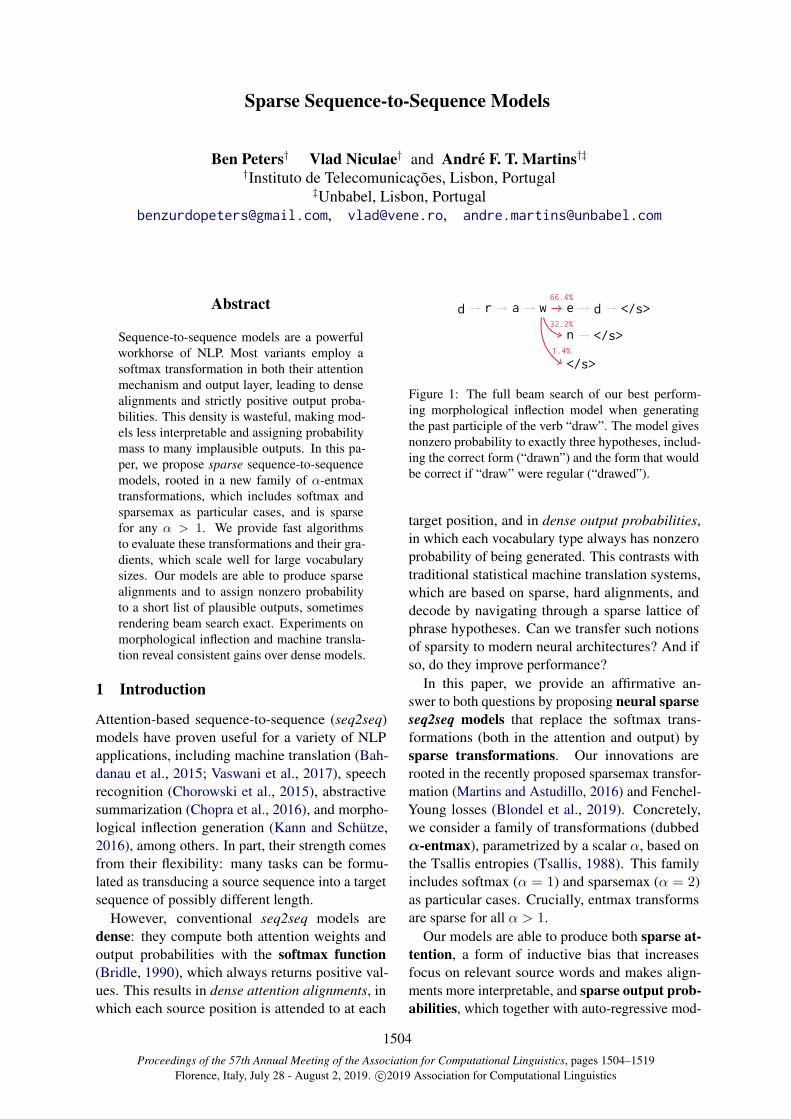
Figure 1: The full beam search of our best perform-

ing morphological inflection model when generating

the past participle of the verb “draw”. The model gives

nonzero probability to exactly three hypotheses, includ-

ing the correct form (“drawn”) and the form that would

be correct if “draw” were regular (“drawed”).

target position, and in dense output probabilities,

in which each vocabulary type always has nonzero

probability of being generated. This contrasts with

traditional statistical machine translation systems,

which are based on sparse, hard alignments, and

decode by navigating through a sparse lattice of

phrase hypotheses. Can we transfer such notions

of sparsity to modern neural architectures? And if

so, do they improve performance?

In this paper, we provide an affirmative an-

swer to both questions by proposing neural sparse

seq2seq models that replace the softmax trans-

formations (both in the attention and output) by

sparse transformations. Our innovations are

rooted in the recently proposed sparsemax transfor-

mation (Martins and Astudillo, 2016) and Fenchel-

Young losses (Blondel et al., 2019). Concretely,

we consider a family of transformations (dubbed

α-entmax), parametrized by a scalar α, based on

the Tsallis entropies (Tsallis, 1988). This family

includes softmax (α = 1) and sparsemax (α = 2)

as particular cases. Crucially, entmax transforms

are sparse for all α > 1.

Our models are able to produce both sparse at-

tention, a form of inductive bias that increases

focus on relevant source words and makes align-

ments more interpretable, and sparse output prob-

abilities, which together with auto-regressive mod-

1505

aton,

ThisSoAndHere

the tree of life .viewlookglimpsekindlookingwayvisiongaze

is another 92.9%

5.9%

1.3%

<0.1%

49.8%

27.1%

19.9%

2.0%

0.9%

0.2%

<0.1%

<0.1%

95.7%

5.9%

1.3%

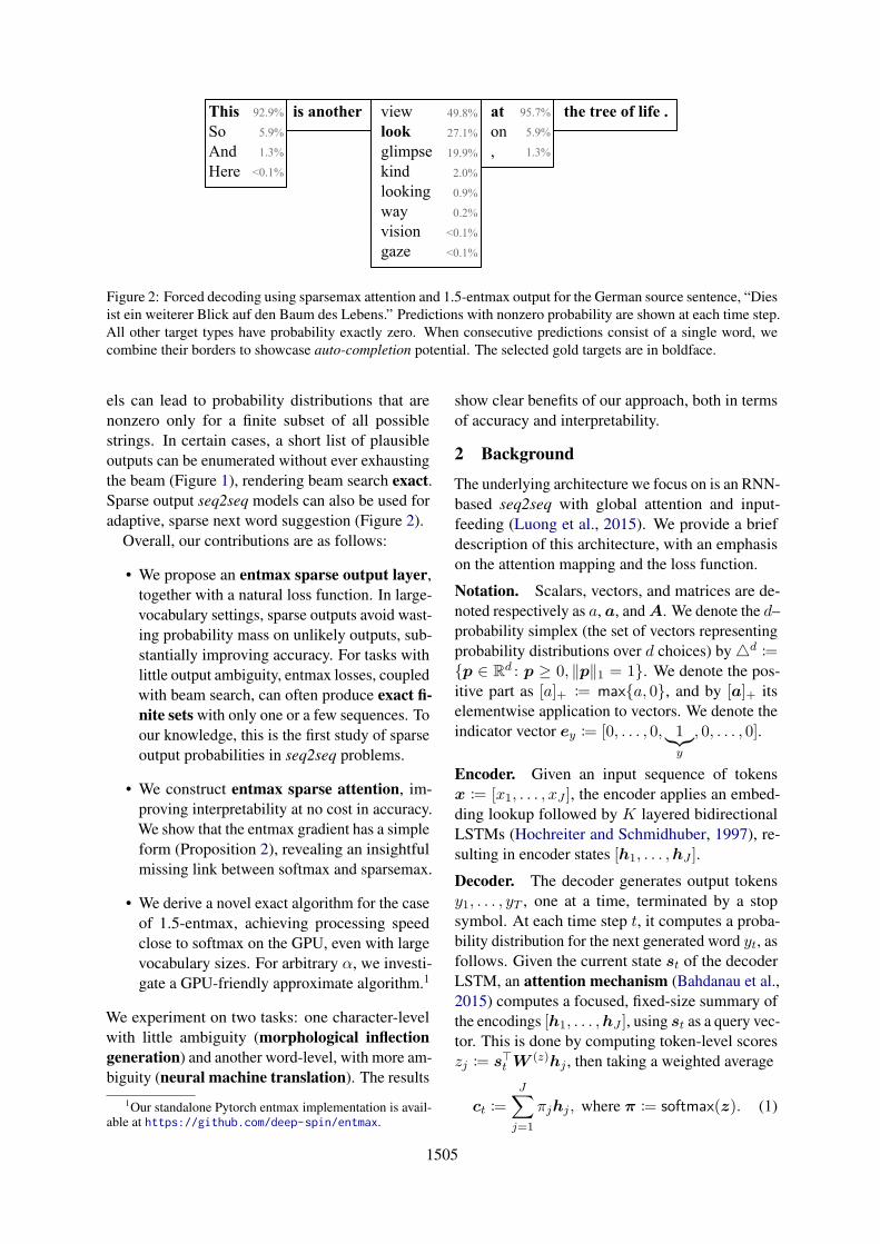
Figure 2: Forced decoding using sparsemax attention and 1.5-entmax output for the German source sentence, “Dies

ist ein weiterer Blick auf den Baum des Lebens.” Predictions with nonzero probability are shown at each time step.

All other target types have probability exactly zero. When consecutive predictions consist of a single word, we

combine their borders to showcase auto-completion potential. The selected gold targets are in boldface.

els can lead to probability distributions that are

nonzero only for a finite subset of all possible

strings. In certain cases, a short list of plausible

outputs can be enumerated without ever exhausting

the beam (Figure 1), rendering beam search exact.

Sparse output seq2seq models can also be used for

adaptive, sparse next word suggestion (Figure 2).

Overall, our contributions are as follows:

• We propose an entmax sparse output layer,

together with a natural loss function. In large-

vocabulary settings, sparse outputs avoid wast-

ing probability mass on unlikely outputs, sub-

stantially improving accuracy. For tasks with

little output ambiguity, entmax losses, coupled

with beam search, can often produce exact fi-

nite sets with only one or a few sequences. To

our knowledge, this is the first study of sparse

output probabilities in seq2seq problems.

• We construct entmax sparse attention, im-

proving interpretability at no cost in accuracy.

We show that the entmax gradient has a simple

form (Proposition 2), revealing an insightful

missing link between softmax and sparsemax.

• We derive a novel exact algorithm for the case

of 1.5-entmax, achieving processing speed

close to softmax on the GPU, even with large

vocabulary sizes. For arbitrary α, we investi-

gate a GPU-friendly approximate algorithm.1

We experiment on two tasks: one character-level

with little ambiguity (morphological inflection

generation) and another word-level, with more am-

biguity (neural machine translation). The results

1Our standalone Pytorch entmax implementation is avail-able at https://github.com/deep-spin/entmax.

show clear benefits of our approach, both in terms

of accuracy and interpretability.

2 Background

The underlying architecture we focus on is an RNN-

based seq2seq with global attention and input-

feeding (Luong et al., 2015). We provide a brief

description of this architecture, with an emphasis

on the attention mapping and the loss function.

Notation. Scalars, vectors, and matrices are de-

noted respectively as a, a, and A. We denote the d–

probability simplex (the set of vectors representing

probability distributions over d choices) by d :=p ∈ Rd : p ≥ 0, ‖p‖1 = 1. We denote the pos-

itive part as [a]+ := maxa, 0, and by [a]+ its

elementwise application to vectors. We denote the

indicator vector ey := [0, . . . , 0, 1︸︷︷︸y

, 0, . . . , 0].

Encoder. Given an input sequence of tokens

x := [x1, . . . , xJ ], the encoder applies an embed-

ding lookup followed by K layered bidirectional

LSTMs (Hochreiter and Schmidhuber, 1997), re-

sulting in encoder states [h1, . . . ,hJ ].

Decoder. The decoder generates output tokens

y1, . . . , yT , one at a time, terminated by a stop

symbol. At each time step t, it computes a proba-

bility distribution for the next generated word yt, as

follows. Given the current state st of the decoder

LSTM, an attention mechanism (Bahdanau et al.,

2015) computes a focused, fixed-size summary of

the encodings [h1, . . . ,hJ ], using st as a query vec-

tor. This is done by computing token-level scores

zj := s⊤t W(z)hj , then taking a weighted average

ct :=J∑

j=1

πjhj , where π := softmax(z). (1)

1506

The contextual output is the non-linear combina-

tion ot := tanh(W (o)[st; ct] + b(o)), yielding the

predictive distribution of the next word

p(yt= · | x, y1, ..., yt−1) := softmax(Vot + b).(2)

The output ot, together with the embedding of the

predicted yt, feed into the decoder LSTM for the

next step, in an auto-regressive manner. The model

is trained to maximize the likelihood of the correct

target sentences, or equivalently, to minimize

L =∑

(x,y)∈D

|y|∑

t=1

(− log softmax(Vot))yt︸ ︷︷ ︸Lsoftmax(yt,Vot)

. (3)

A central building block in the architecture is the

transformation softmax : Rd → d,

softmax(z)j :=exp(zj)∑i exp(zi)

, (4)

which maps a vector of scores z into a probability

distribution (i.e., a vector in d). As seen above,

the softmax mapping plays two crucial roles in the

decoder: first, in computing normalized attention

weights (Eq. 1), second, in computing the predic-

tive probability distribution (Eq. 2). Since exp 0,

softmax never assigns a probability of zero to any

word, so we may never fully rule out non-important

input tokens from attention, nor unlikely words

from the generation vocabulary. While this may

be advantageous for dealing with uncertainty, it

may be preferrable to avoid dedicating model re-

sources to irrelevant words. In the next section, we

present a strategy for differentiable sparse prob-

ability mappings. We show that our approach can

be used to learn powerful seq2seq models with

sparse outputs and sparse attention mechanisms.

3 Sparse Attention and Outputs

3.1 The sparsemax mapping and loss

To pave the way to a more general family of sparse

attention and losses, we point out that softmax

(Eq. 4) is only one of many possible mappings

from Rd to d. Martins and Astudillo (2016) intro-

duce sparsemax: an alternative to softmax which

tends to yield sparse probability distributions:

sparsemax(z) := argminp∈d

‖p− z‖2. (5)

Since Eq. 5 is a projection onto d, which tends

to yield sparse solutions, the predictive distribution

p⋆ := sparsemax(z) is likely to assign exactly

zero probability to low-scoring choices. They also

propose a corresponding loss function to replace

the negative log likelihood loss Lsoftmax (Eq. 3):

Lsparsemax(y, z) :=1

2

(‖ey−z‖2−‖p⋆−z‖2

), (6)

This loss is smooth and convex on z and has a

margin: it is zero if and only if zy ≥ zy′ + 1 for

any y′ 6= y (Martins and Astudillo, 2016, Proposi-

tion 3). Training models with the sparsemax loss

requires its gradient (cf. Appendix A.2):

∇zLsparsemax(y, z) = −ey + p⋆.

For using the sparsemax mapping in an attention

mechanism, Martins and Astudillo (2016) show

that it is differentiable almost everywhere, with

∂ sparsemax(z)

∂z= diag(s)− 1

‖s‖1ss⊤,

where sj = 1 if p⋆j > 0, otherwise sj = 0.

Entropy interpretation. At first glance, sparse-

max appears very different from softmax, and a

strategy for producing other sparse probability map-

pings is not obvious. However, the connection be-

comes clear when considering the variational form

of softmax (Wainwright and Jordan, 2008):

softmax(z) = argmaxp∈d

p⊤z + HS(p), (7)

where HS(p) := −∑j pj log pj is the well-known

Gibbs-Boltzmann-Shannon entropy with base e.

Likewise, letting HG(p) := 12

∑j pj(1− pj) be

the Gini entropy, we can rearrange Eq. 5 as

sparsemax(z) = argmaxp∈d

p⊤z + HG(p), (8)

crystallizing the connection between softmax and

sparsemax: they only differ in the choice of en-

tropic regularizer.

3.2 A new entmax mapping and loss family

The parallel above raises a question: can we find

interesting interpolations between softmax and

sparsemax? We answer affirmatively, by consid-

ering a generalization of the Shannon and Gini

entropies proposed by Tsallis (1988): a family of

entropies parametrized by a scalar α > 1 which we

call Tsallis α-entropies:

HTα(p) :=

1

α(α−1)

∑j

(pj − pαj

), α 6= 1,

HS(p), α = 1.(9)

1507

−2 0 2t

0.0

0.5

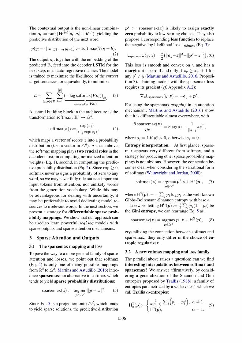
1.0 α = 1 (softmax)α = 1.25α = 1.5α = 2 (sparsemax)α = 4

Figure 3: Illustration of entmax in the two-dimensional

case α-entmax([t, 0])1. All mappings except softmax

saturate at t = ±1/α−1. While sparsemax is piecewise

linear, mappings with 1 < α < 2 have smooth corners.

This family is continuous, i.e., limα→1 HTα(p) =

HS(p) for any p ∈ d (cf. Appendix A.1). More-

over, HT2 ≡ HG. Thus, Tsallis entropies interpolate

between the Shannon and Gini entropies. Starting

from the Tsallis entropies, we construct a probabil-

ity mapping, which we dub entmax:

α-entmax(z) := argmaxp∈d

p⊤z + HTα(p), (10)

and, denoting p⋆ := α-entmax(z), a loss function

Lα(y, z) := (p⋆ − ey)⊤z + HT

α(p⋆) (11)

The motivation for this loss function resides in the

fact that it is a Fenchel-Young loss (Blondel et al.,

2019), as we briefly explain in Appendix A.2. Then,

1-entmax ≡ softmax and 2-entmax ≡ sparsemax.

Similarly, L1 is the negative log likelihood, and

L2 is the sparsemax loss. For all α > 1, entmax

tends to produce sparse probability distributions,

yielding a function family continuously interpolat-

ing between softmax and sparsemax, cf. Figure 3.

The gradient of the entmax loss is

∇zLα(y, z) = −ey + p⋆. (12)

Tsallis entmax losses have useful properties in-

cluding convexity, differentiability, and a hinge-

like separation margin property: the loss incurred

becomes zero when the score of the correct class is

separated by the rest by a margin of 1/α−1. When

separation is achieved, p⋆ = ey (Blondel et al.,

2019). This allows entmax seq2seq models to

be adaptive to the degree of uncertainty present:

decoders may make fully confident predictions at

“easy” time steps, while preserving sparse uncer-

tainty when a few choices are possible (as exem-

plified in Figure 2).

Tsallis entmax probability mappings have not,

to our knowledge, been used in attention mecha-

nisms. They inherit the desirable sparsity of sparse-

max, while exhibiting smoother, differentiable cur-

vature, whereas sparsemax is piecewise linear.

3.3 Computing the entmax mapping

Whether we want to use α-entmax as an attention

mapping, or Lα as a loss function, we must be able

to efficiently compute p⋆ = α-entmax(z), i.e., to

solve the maximization in Eq. 10. For α = 1, the

closed-form solution is given by Eq. 4. For α > 1,

given z, we show that there is a unique threshold τsuch that (Appendix C.1, Lemma 2):

α-entmax(z) = [(α− 1)z − τ1]1/α−1

+ , (13)

i.e., entries with score zj ≤ τ/α−1 get zero prob-

ability. For sparsemax (α = 2), the problem

amounts to Euclidean projection onto d, for

which two types of algorithms are well studied:

i. exact, based on sorting (Held et al., 1974;

Michelot, 1986),

ii. iterative, bisection-based (Liu and Ye, 2009).

The bisection approach searches for the opti-

mal threshold τ numerically. Blondel et al. (2019)

generalize this approach in a way applicable to

α-entmax. The resulting algorithm is (cf. Ap-

pendix C.1 for details):

Algorithm 1 Compute α-entmax by bisection.

1 Define p(τ) := [z − τ ]1/α−1

+ , set z ← (α− 1)z

2 τmin ← max(z)− 1; τmax ← max(z)− d1−α

3 for t ∈ 1, . . . , T do

4 τ ← (τmin + τmax)/2

5 Z ←∑

j pj(τ)

6 if Z < 1 then τmax ← τ else τmin ← τ

7 return 1/Z p(τ)

Algorithm 1 works by iteratively narrowing the

interval containing the exact solution by exactly

half. Line 7 ensures that approximate solutions are

valid probability distributions, i.e., that p⋆ ∈ d.

Although bisection is simple and effective, an ex-

act sorting-based algorithm, like for sparsemax, has

the potential to be faster and more accurate. More-

over, as pointed out by Condat (2016), when exact

solutions are required, it is possible to construct in-

puts z for which bisection requires arbitrarily many

iterations. To address these issues, we propose a

1508

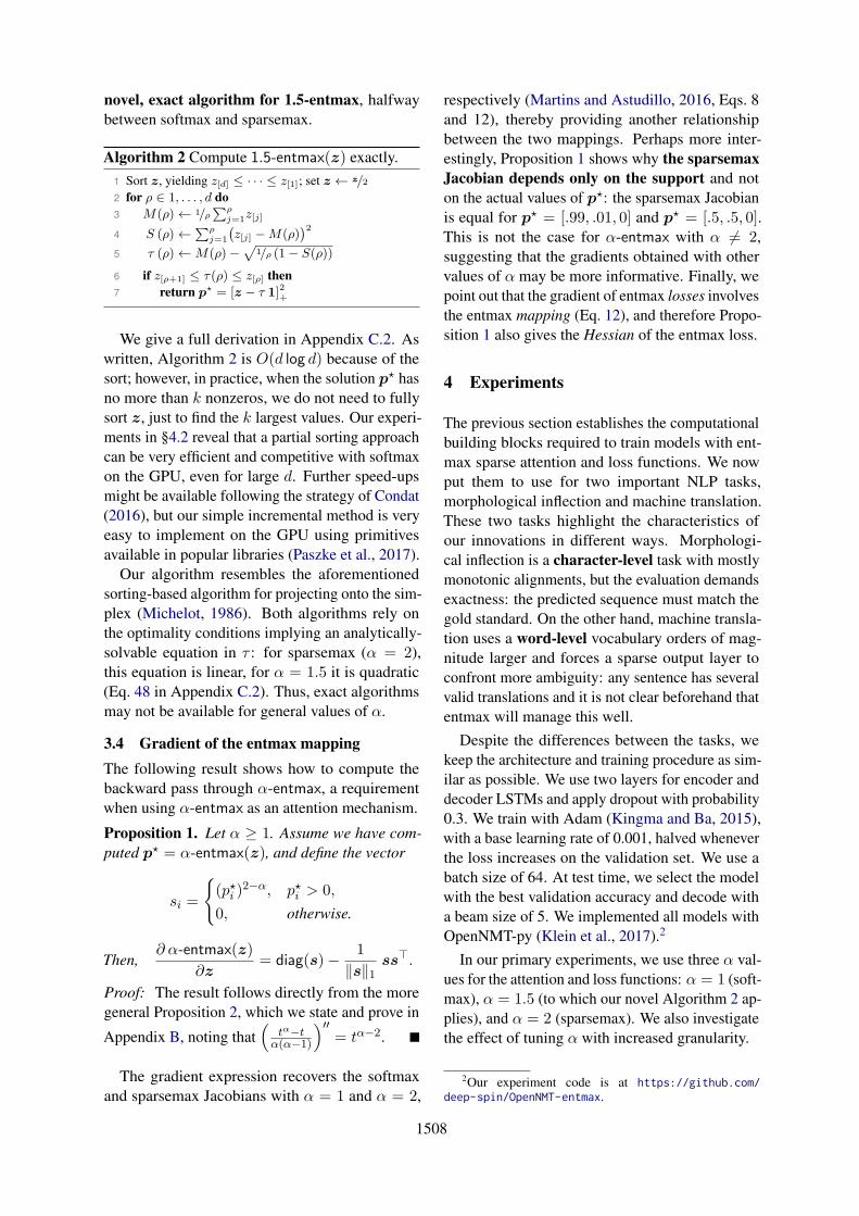
novel, exact algorithm for 1.5-entmax, halfway

between softmax and sparsemax.

Algorithm 2 Compute 1.5-entmax(z) exactly.

1 Sort z, yielding z[d] ≤ · · · ≤ z[1]; set z ← z/2

2 for ρ ∈ 1, . . . , d do

3 M(ρ)← 1/ρ∑ρ

j=1z[j]

4 S (ρ)←∑ρ

j=1

(

z[j] −M(ρ))2

5 τ (ρ)←M(ρ)−√

1/ρ (1− S(ρ))

6 if z[ρ+1] ≤ τ(ρ) ≤ z[ρ] then

7 return p⋆ = [z − τ 1]2+

We give a full derivation in Appendix C.2. As

written, Algorithm 2 is O(d log d) because of the

sort; however, in practice, when the solution p⋆ has

no more than k nonzeros, we do not need to fully

sort z, just to find the k largest values. Our experi-

ments in §4.2 reveal that a partial sorting approach

can be very efficient and competitive with softmax

on the GPU, even for large d. Further speed-ups

might be available following the strategy of Condat

(2016), but our simple incremental method is very

easy to implement on the GPU using primitives

available in popular libraries (Paszke et al., 2017).

Our algorithm resembles the aforementioned

sorting-based algorithm for projecting onto the sim-

plex (Michelot, 1986). Both algorithms rely on

the optimality conditions implying an analytically-

solvable equation in τ : for sparsemax (α = 2),

this equation is linear, for α = 1.5 it is quadratic

(Eq. 48 in Appendix C.2). Thus, exact algorithms

may not be available for general values of α.

3.4 Gradient of the entmax mapping

The following result shows how to compute the

backward pass through α-entmax, a requirement

when using α-entmax as an attention mechanism.

Proposition 1. Let α ≥ 1. Assume we have com-

puted p⋆ = α-entmax(z), and define the vector

si =

(p⋆i )

2−α, p⋆i > 0,

0, otherwise.

Then,∂ α-entmax(z)

∂z= diag(s)− 1

‖s‖1ss⊤.

Proof: The result follows directly from the more

general Proposition 2, which we state and prove in

Appendix B, noting that(

tα−tα(α−1)

)′′= tα−2.

The gradient expression recovers the softmax

and sparsemax Jacobians with α = 1 and α = 2,

respectively (Martins and Astudillo, 2016, Eqs. 8

and 12), thereby providing another relationship

between the two mappings. Perhaps more inter-

estingly, Proposition 1 shows why the sparsemax

Jacobian depends only on the support and not

on the actual values of p⋆: the sparsemax Jacobian

is equal for p⋆ = [.99, .01, 0] and p⋆ = [.5, .5, 0].This is not the case for α-entmax with α 6= 2,

suggesting that the gradients obtained with other

values of α may be more informative. Finally, we

point out that the gradient of entmax losses involves

the entmax mapping (Eq. 12), and therefore Propo-

sition 1 also gives the Hessian of the entmax loss.

4 Experiments

The previous section establishes the computational

building blocks required to train models with ent-

max sparse attention and loss functions. We now

put them to use for two important NLP tasks,

morphological inflection and machine translation.

These two tasks highlight the characteristics of

our innovations in different ways. Morphologi-

cal inflection is a character-level task with mostly

monotonic alignments, but the evaluation demands

exactness: the predicted sequence must match the

gold standard. On the other hand, machine transla-

tion uses a word-level vocabulary orders of mag-

nitude larger and forces a sparse output layer to

confront more ambiguity: any sentence has several

valid translations and it is not clear beforehand that

entmax will manage this well.

Despite the differences between the tasks, we

keep the architecture and training procedure as sim-

ilar as possible. We use two layers for encoder and

decoder LSTMs and apply dropout with probability

0.3. We train with Adam (Kingma and Ba, 2015),

with a base learning rate of 0.001, halved whenever

the loss increases on the validation set. We use a

batch size of 64. At test time, we select the model

with the best validation accuracy and decode with

a beam size of 5. We implemented all models with

OpenNMT-py (Klein et al., 2017).2

In our primary experiments, we use three α val-

ues for the attention and loss functions: α = 1 (soft-

max), α = 1.5 (to which our novel Algorithm 2 ap-

plies), and α = 2 (sparsemax). We also investigate

the effect of tuning α with increased granularity.

2Our experiment code is at https://github.com/

deep-spin/OpenNMT-entmax.

1509

α high mediumoutput attention (avg.) (ens.) (avg.) (ens.)

1 1 93.15 94.20 82.55 85.681.5 92.32 93.50 83.20 85.632 90.98 92.60 83.13 85.65

1.5 1 94.36 94.96 84.88 86.381.5 94.44 95.00 84.93 86.552 94.05 94.74 84.93 86.59

2 1 94.59 95.10 84.95 86.411.5 94.47 95.01 85.03 86.612 94.32 94.89 84.96 86.47

UZH (2018) 96.00 86.64

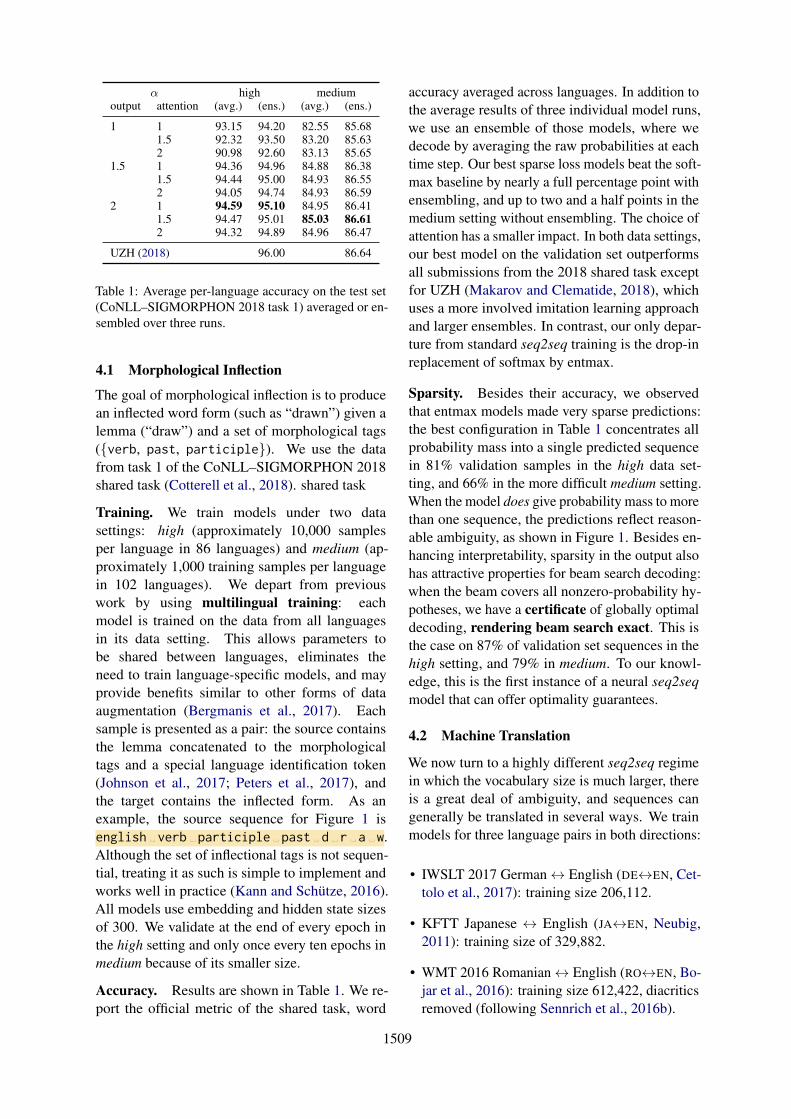
Table 1: Average per-language accuracy on the test set

(CoNLL–SIGMORPHON 2018 task 1) averaged or en-

sembled over three runs.

4.1 Morphological Inflection

The goal of morphological inflection is to produce

an inflected word form (such as “drawn”) given a

lemma (“draw”) and a set of morphological tags

(verb, past, participle). We use the data

from task 1 of the CoNLL–SIGMORPHON 2018

shared task (Cotterell et al., 2018). shared task

Training. We train models under two data

settings: high (approximately 10,000 samples

per language in 86 languages) and medium (ap-

proximately 1,000 training samples per language

in 102 languages). We depart from previous

work by using multilingual training: each

model is trained on the data from all languages

in its data setting. This allows parameters to

be shared between languages, eliminates the

need to train language-specific models, and may

provide benefits similar to other forms of data

augmentation (Bergmanis et al., 2017). Each

sample is presented as a pair: the source contains

the lemma concatenated to the morphological

tags and a special language identification token

(Johnson et al., 2017; Peters et al., 2017), and

the target contains the inflected form. As an

example, the source sequence for Figure 1 is

english verb participle past d r a w.

Although the set of inflectional tags is not sequen-

tial, treating it as such is simple to implement and

works well in practice (Kann and Schutze, 2016).

All models use embedding and hidden state sizes

of 300. We validate at the end of every epoch in

the high setting and only once every ten epochs in

medium because of its smaller size.

Accuracy. Results are shown in Table 1. We re-

port the official metric of the shared task, word

accuracy averaged across languages. In addition to

the average results of three individual model runs,

we use an ensemble of those models, where we

decode by averaging the raw probabilities at each

time step. Our best sparse loss models beat the soft-

max baseline by nearly a full percentage point with

ensembling, and up to two and a half points in the

medium setting without ensembling. The choice of

attention has a smaller impact. In both data settings,

our best model on the validation set outperforms

all submissions from the 2018 shared task except

for UZH (Makarov and Clematide, 2018), which

uses a more involved imitation learning approach

and larger ensembles. In contrast, our only depar-

ture from standard seq2seq training is the drop-in

replacement of softmax by entmax.

Sparsity. Besides their accuracy, we observed

that entmax models made very sparse predictions:

the best configuration in Table 1 concentrates all

probability mass into a single predicted sequence

in 81% validation samples in the high data set-

ting, and 66% in the more difficult medium setting.

When the model does give probability mass to more

than one sequence, the predictions reflect reason-

able ambiguity, as shown in Figure 1. Besides en-

hancing interpretability, sparsity in the output also

has attractive properties for beam search decoding:

when the beam covers all nonzero-probability hy-

potheses, we have a certificate of globally optimal

decoding, rendering beam search exact. This is

the case on 87% of validation set sequences in the

high setting, and 79% in medium. To our knowl-

edge, this is the first instance of a neural seq2seq

model that can offer optimality guarantees.

4.2 Machine Translation

We now turn to a highly different seq2seq regime

in which the vocabulary size is much larger, there

is a great deal of ambiguity, and sequences can

generally be translated in several ways. We train

models for three language pairs in both directions:

• IWSLT 2017 German ↔ English (DE↔EN, Cet-

tolo et al., 2017): training size 206,112.

• KFTT Japanese ↔ English (JA↔EN, Neubig,

2011): training size of 329,882.

• WMT 2016 Romanian ↔ English (RO↔EN, Bo-

jar et al., 2016): training size 612,422, diacritics

removed (following Sennrich et al., 2016b).

1510

method DEEN ENDE JAEN ENJA ROEN ENRO

softmax 25.70 ± 0.15 21.86 ± 0.09 20.22 ± 0.08 25.21 ± 0.29 29.12 ± 0.18 28.12 ± 0.181.5-entmax 26.17 ± 0.13 22.42 ± 0.08 20.55 ± 0.30 26.00 ± 0.31 30.15 ± 0.06 28.84 ± 0.10sparsemax 24.69 ± 0.22 20.82 ± 0.19 18.54 ± 0.11 23.84 ± 0.37 29.20 ± 0.16 28.03 ± 0.16

Table 2: Machine translation comparison of softmax, sparsemax, and the proposed 1.5-entmax as both attention

mapping and loss function. Reported is tokenized test BLEU averaged across three runs (higher is better).

Training. We use byte pair encoding (BPE; Sen-

nrich et al., 2016a) to ensure an open vocabulary.

We use separate segmentations with 25k merge

operations per language for RO↔EN and a joint

segmentation with 32k merges for the other lan-

guage pairs. DE↔EN is validated once every 5k

steps because of its smaller size, while the other

sets are validated once every 10k steps. We set

the maximum number of training steps at 120k for

RO↔EN and 100k for other language pairs. We use

500 dimensions for word vectors and hidden states.

Evaluation. Table 2 shows BLEU scores (Pa-

pineni et al., 2002) for the three models with

α ∈ 1, 1.5, 2, using the same value of α for the

attention mechanism and loss function. We observe

that the 1.5-entmax configuration consistently per-

forms best across all six choices of language pair

and direction. These results support the notion

that the optimal function is somewhere between

softmax and sparsemax, which motivates a more

fine-grained search for α; we explore this next.

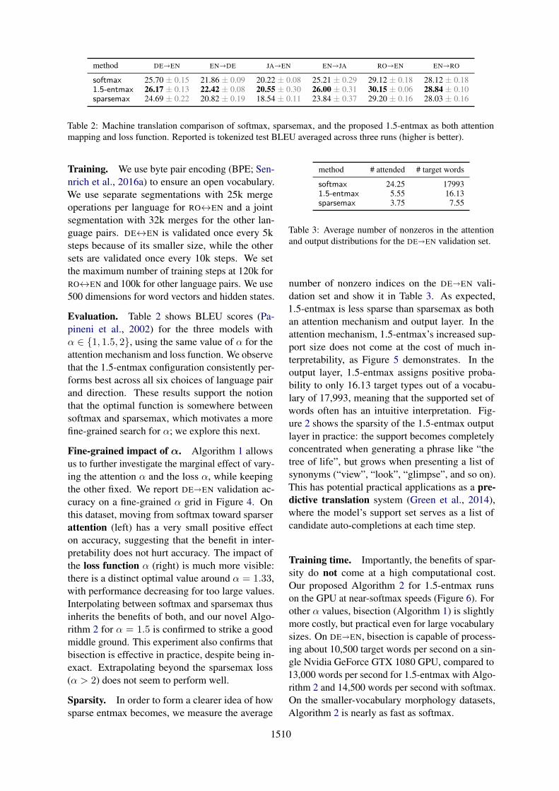
Fine-grained impact of α. Algorithm 1 allows

us to further investigate the marginal effect of vary-

ing the attention α and the loss α, while keeping

the other fixed. We report DEEN validation ac-

curacy on a fine-grained α grid in Figure 4. On

this dataset, moving from softmax toward sparser

attention (left) has a very small positive effect

on accuracy, suggesting that the benefit in inter-

pretability does not hurt accuracy. The impact of

the loss function α (right) is much more visible:

there is a distinct optimal value around α = 1.33,

with performance decreasing for too large values.

Interpolating between softmax and sparsemax thus

inherits the benefits of both, and our novel Algo-

rithm 2 for α = 1.5 is confirmed to strike a good

middle ground. This experiment also confirms that

bisection is effective in practice, despite being in-

exact. Extrapolating beyond the sparsemax loss

(α > 2) does not seem to perform well.

Sparsity. In order to form a clearer idea of how

sparse entmax becomes, we measure the average

method # attended # target words

softmax 24.25 179931.5-entmax 5.55 16.13sparsemax 3.75 7.55

Table 3: Average number of nonzeros in the attention

and output distributions for the DEEN validation set.

number of nonzero indices on the DEEN vali-

dation set and show it in Table 3. As expected,

1.5-entmax is less sparse than sparsemax as both

an attention mechanism and output layer. In the

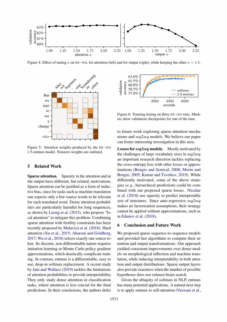
attention mechanism, 1.5-entmax’s increased sup-

port size does not come at the cost of much in-

terpretability, as Figure 5 demonstrates. In the

output layer, 1.5-entmax assigns positive proba-

bility to only 16.13 target types out of a vocabu-

lary of 17,993, meaning that the supported set of

words often has an intuitive interpretation. Fig-

ure 2 shows the sparsity of the 1.5-entmax output

layer in practice: the support becomes completely

concentrated when generating a phrase like “the

tree of life”, but grows when presenting a list of

synonyms (“view”, “look”, “glimpse”, and so on).

This has potential practical applications as a pre-

dictive translation system (Green et al., 2014),

where the model’s support set serves as a list of

candidate auto-completions at each time step.

Training time. Importantly, the benefits of spar-

sity do not come at a high computational cost.

Our proposed Algorithm 2 for 1.5-entmax runs

on the GPU at near-softmax speeds (Figure 6). For

other α values, bisection (Algorithm 1) is slightly

more costly, but practical even for large vocabulary

sizes. On DEEN, bisection is capable of process-

ing about 10,500 target words per second on a sin-

gle Nvidia GeForce GTX 1080 GPU, compared to

13,000 words per second for 1.5-entmax with Algo-

rithm 2 and 14,500 words per second with softmax.

On the smaller-vocabulary morphology datasets,

Algorithm 2 is nearly as fast as softmax.

1511

1.00 1.25 1.50 1.75 2.00 2.25attention α

60%

61%

62%

63%val

idat

ion

accu

racy

1.00 1.25 1.50 1.75 2.00 2.25output α

Figure 4: Effect of tuning α on DEEN, for attention (left) and for output (right), while keeping the other α = 1.5.

Abe

r

wir

begi

nnen

, eine

Verän

deru

ng

zu sehe

n

.

But

we

start

to

see

a

change

.

</s>

Figure 5: Attention weights produced by the DEEN

1.5-entmax model. Nonzero weights are outlined.

5 Related Work

Sparse attention. Sparsity in the attention and in

the output have different, but related, motivations.

Sparse attention can be justified as a form of induc-

tive bias, since for tasks such as machine translation

one expects only a few source words to be relevant

for each translated word. Dense attention probabil-

ities are particularly harmful for long sequences,

as shown by Luong et al. (2015), who propose “lo-

cal attention” to mitigate this problem. Combining

sparse attention with fertility constraints has been

recently proposed by Malaviya et al. (2018). Hard

attention (Xu et al., 2015; Aharoni and Goldberg,

2017; Wu et al., 2018) selects exactly one source to-

ken. Its discrete, non-differentiable nature requires

imitation learning or Monte Carlo policy gradient

approximations, which drastically complicate train-

ing. In contrast, entmax is a differentiable, easy to

use, drop-in softmax replacement. A recent study

by Jain and Wallace (2019) tackles the limitations

of attention probabilities to provide interpretability.

They only study dense attention in classification

tasks, where attention is less crucial for the final

predictions. In their conclusions, the authors defer

2000 4000 6000seconds

57.0%58.5%60.0%61.5%63.0%

val

idat

ion

accu

racy

softmax

1.5-entmax

Figure 6: Training timing on three DEEN runs. Mark-

ers show validation checkpoints for one of the runs.

to future work exploring sparse attention mecha-

nisms and seq2seq models. We believe our paper

can foster interesting investigation in this area.

Losses for seq2seq models. Mostly motivated by

the challenges of large vocabulary sizes in seq2seq,

an important research direction tackles replacing

the cross-entropy loss with other losses or approx-

imations (Bengio and Senecal, 2008; Morin and

Bengio, 2005; Kumar and Tsvetkov, 2019). While

differently motivated, some of the above strate-

gies (e.g., hierarchical prediction) could be com-

bined with our proposed sparse losses. Niculae

et al. (2018) use sparsity to predict interpretable

sets of structures. Since auto-regressive seq2seq

makes no factorization assumptions, their strategy

cannot be applied without approximations, such as

in Edunov et al. (2018).

6 Conclusion and Future Work

We proposed sparse sequence-to-sequence models

and provided fast algorithms to compute their at-

tention and output transformations. Our approach

yielded consistent improvements over dense mod-

els on morphological inflection and machine trans-

lation, while inducing interpretability in both atten-

tion and output distributions. Sparse output layers

also provide exactness when the number of possible

hypotheses does not exhaust beam search.

Given the ubiquity of softmax in NLP, entmax

has many potential applications. A natural next step

is to apply entmax to self-attention (Vaswani et al.,

1512

2017). In a different vein, the strong morphological

inflection results point to usefulness in other tasks

where probability is concentrated in a small number

of hypotheses, such as speech recognition.

Acknowledgments

This work was supported by the European Re-

search Council (ERC StG DeepSPIN 758969),

and by the Fundacao para a Ciencia e Tecnolo-

gia through contracts UID/EEA/50008/2019 and

CMUPERI/TIC/0046/2014 (GoLocal). We thank

Mathieu Blondel, Nikolay Bogoychev, Goncalo

Correia, Erick Fonseca, Pedro Martins, Tsvetomila

Mihaylova, Miguel Rios, Marcos Treviso, and the

anonymous reviewers, for helpful discussion and

feedback.

References

Roee Aharoni and Yoav Goldberg. 2017. Morphologi-cal inflection generation with hard monotonic atten-tion. In Proc. ACL.

Dzmitry Bahdanau, Kyunghyun Cho, and Yoshua Ben-gio. 2015. Neural machine translation by jointlylearning to align and translate. In Proc. ICLR.

Yoshua Bengio and Jean-Sebastien Senecal. 2008.Adaptive importance sampling to accelerate train-ing of a neural probabilistic language model. IEEETransactions on Neural Networks, 19(4):713–722.

Toms Bergmanis, Katharina Kann, Hinrich Schutze,and Sharon Goldwater. 2017. Training data augmen-tation for low-resource morphological inflection. InProc. CoNLL–SIGMORPHON.

Mathieu Blondel, Andre FT Martins, and Vlad Nicu-lae. 2019. Learning classifiers with Fenchel-Younglosses: Generalized entropies, margins, and algo-rithms. In Proc. AISTATS.

Ondrej Bojar, Rajen Chatterjee, Christian Federmann,Yvette Graham, Barry Haddow, Matthias Huck, An-tonio Jimeno Yepes, Philipp Koehn, Varvara Lo-gacheva, Christof Monz, et al. 2016. Findings ofthe 2016 conference on machine translation. In ACLWMT.

John S Bridle. 1990. Probabilistic interpretation offeedforward classification network outputs, with re-lationships to statistical pattern recognition. In Neu-rocomputing, pages 227–236. Springer.

M Cettolo, M Federico, L Bentivogli, J Niehues,S Stuker, K Sudoh, K Yoshino, and C Federmann.2017. Overview of the IWSLT 2017 evaluation cam-paign. In Proc. IWSLT.

Sumit Chopra, Michael Auli, and Alexander M Rush.2016. Abstractive sentence summarization with at-tentive recurrent neural networks. In Proc. NAACL-HLT.

Jan K Chorowski, Dzmitry Bahdanau, DmitriySerdyuk, Kyunghyun Cho, and Yoshua Bengio.2015. Attention-based models for speech recogni-tion. In Proc. NeurIPS.

Laurent Condat. 2016. Fast projection onto the simplexand the ℓ1 ball. Mathematical Programming, 158(1-2):575–585.

Ryan Cotterell, Christo Kirov, John Sylak-Glassman,Geraldine Walther, Ekaterina Vylomova, Arya DMcCarthy, Katharina Kann, Sebastian Mielke, Gar-rett Nicolai, Miikka Silfverberg, et al. 2018. TheCoNLL–SIGMORPHON 2018 shared task: Uni-versal morphological reinflection. Proc. CoNLL–SIGMORPHON.

John M Danskin. 1966. The theory of max-min, withapplications. SIAM Journal on Applied Mathemat-ics, 14(4):641–664.

Sergey Edunov, Myle Ott, Michael Auli, David Grang-ier, et al. 2018. Classical structured prediction lossesfor sequence to sequence learning. In Proc. NAACL-HLT.

Spence Green, Sida I Wang, Jason Chuang, JeffreyHeer, Sebastian Schuster, and Christopher D Man-ning. 2014. Human effort and machine learnabilityin computer aided translation. In Proc. EMNLP.

Michael Held, Philip Wolfe, and Harlan P Crowder.1974. Validation of subgradient optimization. Math-ematical Programming, 6(1):62–88.

Sepp Hochreiter and Jurgen Schmidhuber. 1997.Long short-term memory. Neural Computation,9(8):1735–1780.

Sarthak Jain and Byron C. Wallace. 2019. Attention isnot explanation. In Proc. NAACL-HLT.

Melvin Johnson, Mike Schuster, Quoc V Le, MaximKrikun, Yonghui Wu, Zhifeng Chen, Nikhil Thorat,Fernanda Viegas, Martin Wattenberg, Greg Corrado,et al. 2017. Google’s multilingual neural machinetranslation system: Enabling zero-shot translation.Transactions of the Association for ComputationalLinguistics, 5:339–351.

Katharina Kann and Hinrich Schutze. 2016. MED: TheLMU system for the SIGMORPHON 2016 sharedtask on morphological reinflection. In Proc. SIG-MORPHON.

Diederik Kingma and Jimmy Ba. 2015. Adam: Amethod for stochastic optimization. In Proc. ICLR.

Guillaume Klein, Yoon Kim, Yuntian Deng, Jean Senel-lart, and Alexander M Rush. 2017. OpenNMT:Open-source toolkit for neural machine translation.arXiv e-prints.

1513

Sachin Kumar and Yulia Tsvetkov. 2019. Von Mises-Fisher loss for training sequence to sequence modelswith continuous outputs. In Proc. ICLR.

Jun Liu and Jieping Ye. 2009. Efficient Euclidean pro-jections in linear time. In Proc. ICML.

Minh-Thang Luong, Hieu Pham, and Christopher DManning. 2015. Effective approaches to attention-based neural machine translation. In Proc. EMNLP.

Peter Makarov and Simon Clematide. 2018. UZH atCoNLL–SIGMORPHON 2018 shared task on uni-versal morphological reinflection. Proc. CoNLL–SIGMORPHON.

Chaitanya Malaviya, Pedro Ferreira, and Andre FTMartins. 2018. Sparse and constrained attention forneural machine translation. In Proc. ACL.

Andre FT Martins and Ramon Fernandez Astudillo.2016. From softmax to sparsemax: A sparse modelof attention and multi-label classification. In Proc.of ICML.

Christian Michelot. 1986. A finite algorithm for find-ing the projection of a point onto the canonical sim-plex of Rn. Journal of Optimization Theory and Ap-plications, 50(1):195–200.

Frederic Morin and Yoshua Bengio. 2005. Hierarchi-cal probabilistic neural network language model. InProc. AISTATS.

Graham Neubig. 2011. The Kyoto free translation task.http://www.phontron.com/kftt.

Vlad Niculae and Mathieu Blondel. 2017. A regular-ized framework for sparse and structured neural at-tention. In Proc. NeurIPS.

Vlad Niculae, Andre FT Martins, Mathieu Blondel, andClaire Cardie. 2018. SparseMAP: Differentiablesparse structured inference. In Proc. ICML.

Kishore Papineni, Salim Roukos, Todd Ward, and Wei-Jing Zhu. 2002. BLEU: a method for automatic eval-uation of machine translation. In Proc. ACL.

Adam Paszke, Sam Gross, Soumith Chintala, GregoryChanan, Edward Yang, Zachary DeVito, ZemingLin, Alban Desmaison, Luca Antiga, and AdamLerer. 2017. Automatic differentiation in PyTorch.In Proc. NeurIPS Autodiff Workshop.

Ben Peters, Jon Dehdari, and Josef van Genabith.2017. Massively multilingual neural grapheme-to-phoneme conversion. In Proc. Workshop on Build-ing Linguistically Generalizable NLP Systems.

R Tyrrell Rockafellar. 1970. Convex Analysis. Prince-ton University Press.

Rico Sennrich, Barry Haddow, and Alexandra Birch.2016a. Neural machine translation of rare wordswith subword units. In Proc. ACL.

Rico Sennrich, Barry Haddow, and Alexandra Birch.2016b. Edinburgh neural machine translation sys-tems for WMT 16. In Proc. WMT.

Constantino Tsallis. 1988. Possible generalization ofBoltzmann-Gibbs statistics. Journal of StatisticalPhysics, 52:479–487.

Ashish Vaswani, Noam Shazeer, Niki Parmar, JakobUszkoreit, Llion Jones, Aidan N Gomez, ŁukaszKaiser, and Illia Polosukhin. 2017. Attention is allyou need. In Proc. NeurIPS.

Martin J Wainwright and Michael I Jordan. 2008.Graphical models, exponential families, and varia-tional inference. Foundations and Trends® in Ma-chine Learning, 1(1–2):1–305.

Shijie Wu, Pamela Shapiro, and Ryan Cotterell. 2018.Hard non-monotonic attention for character-leveltransduction. In Proc. EMNLP.

Kelvin Xu, Jimmy Ba, Ryan Kiros, Kyunghyun Cho,Aaron Courville, Ruslan Salakhudinov, Rich Zemel,and Yoshua Bengio. 2015. Show, attend and tell:Neural image caption generation with visual atten-tion. In Proc. ICML.

1514

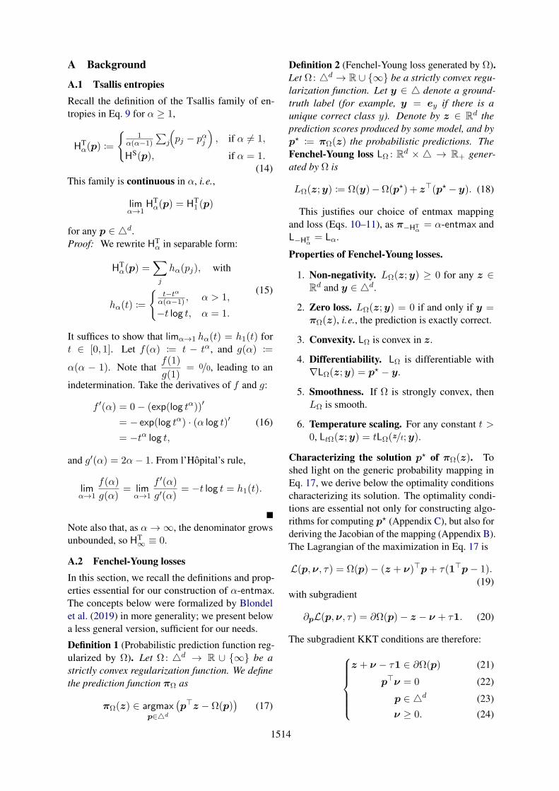
A Background

A.1 Tsallis entropies

Recall the definition of the Tsallis family of en-

tropies in Eq. 9 for α ≥ 1,

HTα(p) :=

1

α(α−1)

∑j

(pj − pαj

), if α 6= 1,

HS(p), if α = 1.(14)

This family is continuous in α, i.e.,

limα→1

HTα(p) = HT

1 (p)

for any p ∈ d.

Proof: We rewrite HTα in separable form:

HTα(p) =

∑

j

hα(pj), with

hα(t) :=

t−tα

α(α−1) , α > 1,

−t log t, α = 1.

(15)

It suffices to show that limα→1 hα(t) = h1(t) for

t ∈ [0, 1]. Let f(α) := t − tα, and g(α) :=

α(α − 1). Note thatf(1)

g(1)= 0/0, leading to an

indetermination. Take the derivatives of f and g:

f ′(α) = 0− (exp(log tα))′

= − exp(log tα) · (α log t)′

= −tα log t,

(16)

and g′(α) = 2α− 1. From l’Hopital’s rule,

limα→1

f(α)

g(α)= lim

α→1

f ′(α)

g′(α)= −t log t = h1(t).

Note also that, as α → ∞, the denominator grows

unbounded, so HT∞ ≡ 0.

A.2 Fenchel-Young losses

In this section, we recall the definitions and prop-

erties essential for our construction of α-entmax.

The concepts below were formalized by Blondel

et al. (2019) in more generality; we present below

a less general version, sufficient for our needs.

Definition 1 (Probabilistic prediction function reg-

ularized by Ω). Let Ω: d → R ∪ ∞ be a

strictly convex regularization function. We define

the prediction function πΩ as

πΩ(z) ∈ argmaxp∈d

(p⊤z − Ω(p)

)(17)

Definition 2 (Fenchel-Young loss generated by Ω).

Let Ω: d → R ∪ ∞ be a strictly convex regu-

larization function. Let y ∈ denote a ground-

truth label (for example, y = ey if there is a

unique correct class y). Denote by z ∈ Rd the

prediction scores produced by some model, and by

p⋆ := πΩ(z) the probabilistic predictions. The

Fenchel-Young loss LΩ : Rd × → R+ gener-

ated by Ω is

LΩ(z;y) := Ω(y)−Ω(p⋆) + z⊤(p⋆ − y). (18)

This justifies our choice of entmax mapping

and loss (Eqs. 10–11), as π−HTα= α-entmax and

L−HTα= Lα.

Properties of Fenchel-Young losses.

1. Non-negativity. LΩ(z;y) ≥ 0 for any z ∈Rd and y ∈ d.

2. Zero loss. LΩ(z;y) = 0 if and only if y =πΩ(z), i.e., the prediction is exactly correct.

3. Convexity. LΩ is convex in z.

4. Differentiability. LΩ is differentiable with

∇LΩ(z;y) = p⋆ − y.

5. Smoothness. If Ω is strongly convex, then

LΩ is smooth.

6. Temperature scaling. For any constant t >0, LtΩ(z;y) = tLΩ(z/t;y).

Characterizing the solution p⋆ of πΩ(z). To

shed light on the generic probability mapping in

Eq. 17, we derive below the optimality conditions

characterizing its solution. The optimality condi-

tions are essential not only for constructing algo-

rithms for computing p⋆ (Appendix C), but also for

deriving the Jacobian of the mapping (Appendix B).

The Lagrangian of the maximization in Eq. 17 is

L(p,ν, τ) = Ω(p)− (z + ν)⊤p+ τ(1⊤p− 1).(19)

with subgradient

∂pL(p,ν, τ) = ∂Ω(p)− z − ν + τ1. (20)

The subgradient KKT conditions are therefore:

z + ν − τ1 ∈ ∂Ω(p)

p⊤ν = 0

p ∈ d

ν ≥ 0.

(21)

(22)

(23)

(24)

1515

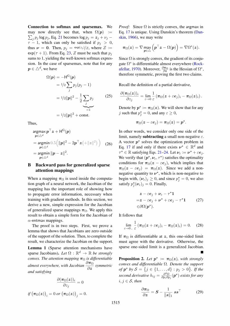
Connection to softmax and sparsemax. We

may now directly see that, when Ω(p) :=∑j pj log pj , Eq. 21 becomes log pj = zj + νj −

τ − 1, which can only be satisfied if pj > 0,

thus ν = 0. Then, pj = exp(zj)/Z, where Z :=exp(τ + 1). From Eq. 23, Z must be such that pjsums to 1, yielding the well-known softmax expres-

sion. In the case of sparsemax, note that for any

p ∈ d, we have

Ω(p) = −HG(p)

= 1/2∑

j

pj(pj − 1)

= 1/2‖p‖2 − 1

2

∑

j

pj

︸ ︷︷ ︸=1

= 1/2‖p‖2 + const.

(25)

Thus,

argmaxp∈d

p⊤z + HG(p)

= argminp∈d

0.5(‖p‖2 − 2p⊤z

(+‖z‖2

) )

= argminp∈d

‖p− z‖2.

(26)

B Backward pass for generalized sparse

attention mappings

When a mapping πΩ is used inside the computa-

tion graph of a neural network, the Jacobian of the

mapping has the important role of showing how

to propagate error information, necessary when

training with gradient methods. In this section, we

derive a new, simple expression for the Jacobian

of generalized sparse mappings πΩ. We apply this

result to obtain a simple form for the Jacobian of

α-entmax mappings.

The proof is in two steps. First, we prove a

lemma that shows that Jacobians are zero outside

of the support of the solution. Then, to complete the

result, we characterize the Jacobian on the support.

Lemma 1 (Sparse attention mechanisms have

sparse Jacobians). Let Ω : Rd → R be strongly

convex. The attention mapping πΩ is differentiable

almost everywhere, with Jacobian∂πΩ

∂zsymmetric

and satisfying

∂(πΩ(z))i∂zj

= 0

if(πΩ(z)

)i= 0 or

(πΩ(z)

)j= 0.

Proof: Since Ω is strictly convex, the argmax in

Eq. 17 is unique. Using Danskin’s theorem (Dan-

skin, 1966), we may write

πΩ(z) = ∇maxp∈

(p⊤z − Ω(p)

)= ∇Ω∗(z).

Since Ω is strongly convex, the gradient of its conju-

gate Ω∗ is differentiable almost everywhere (Rock-

afellar, 1970). Moreover, ∂πΩ∂z is the Hessian of Ω∗,

therefore symmetric, proving the first two claims.

Recall the definition of a partial derivative,

∂(πΩ(z))i∂zj

= limε→0

1

ε(πΩ(z + εej)i − πΩ(z)i) .

Denote by p⋆ := πΩ(z). We will show that for any

j such that p⋆j = 0, and any ε ≥ 0,

πΩ(z − εej) = πΩ(z) = p⋆.

In other words, we consider only one side of the

limit, namely subtracting a small non-negative ε.

A vector p⋆ solves the optimization problem in

Eq. 17 if and only if there exists ν⋆ ∈ Rd and

τ⋆ ∈ R satisfying Eqs. 21–24. Let νε := ν⋆ + εej .

We verify that (p⋆,νε, τ⋆) satisfies the optimality

conditions for πΩ(z − εej), which implies that

πΩ(z − εej) = πΩ(z). Since we add a non-

negative quantity to ν⋆, which is non-negative to

begin with, (νε)j ≥ 0, and since p⋆j = 0, we also

satisfy p⋆j (νε)j = 0. Finally,

z − εej + νε − τ⋆1

=z − εej + ν⋆ + εej − τ⋆1

∈∂Ω(p⋆).

(27)

It follows that

limε→0−

1

ε(πΩ(z + εej)i − πΩ(z)i) = 0. (28)

If πΩ is differentiable at z, this one-sided limit

must agree with the derivative. Otherwise, the

sparse one-sided limit is a generalized Jacobian.

Proposition 2. Let p⋆ := πΩ(z), with strongly

convex and differentiable Ω. Denote the support

of p⋆ by S =j ∈ 1, . . . , d : pj > 0

. If the

second derivative hij =∂2Ω

∂pi∂pj(p⋆) exists for any

i, j ∈ S , then

∂πΩ

∂z= S − 1

‖s‖1ss⊤ (29)

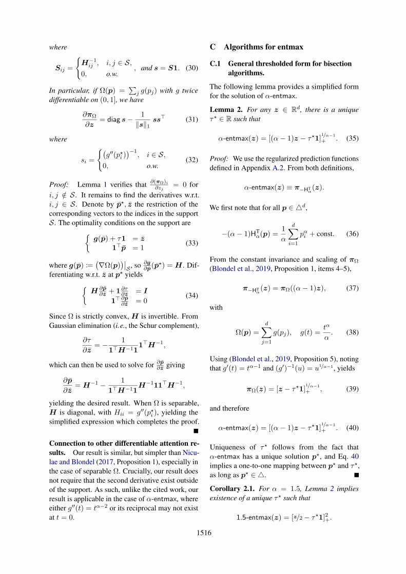
1516

where

Sij =

H−1

ij , i, j ∈ S,0, o.w.

, and s = S1. (30)

In particular, if Ω(p) =∑

j g(pj) with g twice

differentiable on (0, 1], we have

∂πΩ

∂z= diag s− 1

‖s‖1ss⊤ (31)

where

si =

(g′′(p⋆i )

)−1, i ∈ S,

0, o.w.(32)

Proof: Lemma 1 verifies that∂(πΩ)i∂zj

= 0 for

i, j /∈ S. It remains to find the derivatives w.r.t.

i, j ∈ S. Denote by p⋆, z the restriction of the

corresponding vectors to the indices in the support

S . The optimality conditions on the support are

g(p) + τ1 = z

1⊤p = 1

(33)

where g(p) :=(∇Ω(p)

)∣∣S

, so ∂g∂p(p

⋆) = H . Dif-

ferentiating w.r.t. z at p⋆ yields

H ∂p

∂z + 1∂τ∂z = I

1⊤ ∂p

∂z = 0(34)

Since Ω is strictly convex, H is invertible. From

Gaussian elimination (i.e., the Schur complement),

∂τ

∂z= − 1

1⊤H−111⊤H−1,

which can then be used to solve for ∂p∂z giving

∂p

∂z= H−1 − 1

1⊤H−11H−1

11⊤H−1,

yielding the desired result. When Ω is separable,

H is diagonal, with Hii = g′′(p⋆i ), yielding the

simplified expression which completes the proof.

Connection to other differentiable attention re-

sults. Our result is similar, but simpler than Nicu-

lae and Blondel (2017, Proposition 1), especially in

the case of separable Ω. Crucially, our result does

not require that the second derivative exist outside

of the support. As such, unlike the cited work, our

result is applicable in the case of α-entmax, where

either g′′(t) = tα−2 or its reciprocal may not exist

at t = 0.

C Algorithms for entmax

C.1 General thresholded form for bisection

algorithms.

The following lemma provides a simplified form

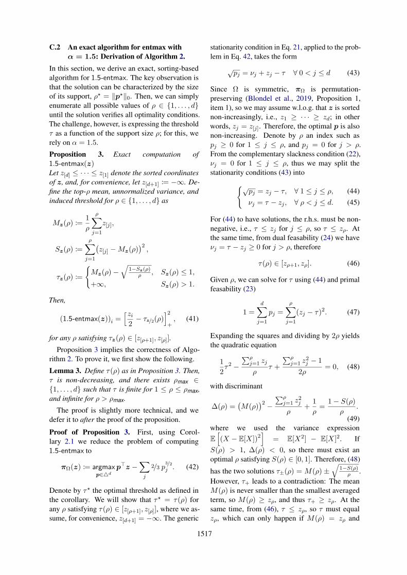
for the solution of α-entmax.

Lemma 2. For any z ∈ Rd, there is a unique

τ⋆ ∈ R such that

α-entmax(z) = [(α− 1)z − τ⋆1]1/α−1

+ . (35)

Proof: We use the regularized prediction functions

defined in Appendix A.2. From both definitions,

α-entmax(z) ≡ π−HTα(z).

We first note that for all p ∈ d,

−(α− 1)HTα(p) =

1

α

d∑

i=1

pαi + const. (36)

From the constant invariance and scaling of πΩ

(Blondel et al., 2019, Proposition 1, items 4–5),

π−HTα(z) = πΩ((α− 1)z), (37)

with

Ω(p) =d∑

j=1

g(pj), g(t) =tα

α. (38)

Using (Blondel et al., 2019, Proposition 5), noting

that g′(t) = tα−1 and (g′)−1(u) = u1/α−1, yields

πΩ(z) = [z − τ⋆1]1/α−1

+ , (39)

and therefore

α-entmax(z) = [(α− 1)z − τ⋆1]1/α−1

+ . (40)

Uniqueness of τ⋆ follows from the fact that

α-entmax has a unique solution p⋆, and Eq. 40

implies a one-to-one mapping between p⋆ and τ⋆,

as long as p⋆ ∈ .

Corollary 2.1. For α = 1.5, Lemma 2 implies

existence of a unique τ⋆ such that

1.5-entmax(z) = [z/2 − τ⋆1]2+.

1517

C.2 An exact algorithm for entmax with

α = 1.5: Derivation of Algorithm 2.

In this section, we derive an exact, sorting-based

algorithm for 1.5-entmax. The key observation is

that the solution can be characterized by the size

of its support, ρ⋆ = ‖p⋆‖0. Then, we can simply

enumerate all possible values of ρ ∈ 1, . . . , duntil the solution verifies all optimality conditions.

The challenge, however, is expressing the threshold

τ as a function of the support size ρ; for this, we

rely on α = 1.5.

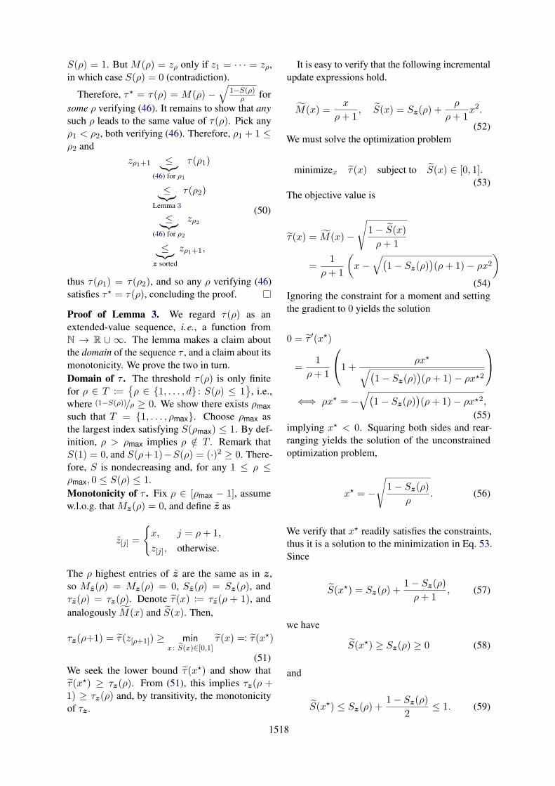
Proposition 3. Exact computation of

1.5-entmax(z)Let z[d] ≤ · · · ≤ z[1] denote the sorted coordinates

of z, and, for convenience, let z[d+1] := −∞. De-

fine the top-ρ mean, unnormalized variance, and

induced threshold for ρ ∈ 1, . . . , d as

Mz(ρ) :=1

ρ

ρ∑

j=1

z[j],

Sz(ρ) :=

ρ∑

j=1

(z[j] −Mz(ρ)

)2,

τz(ρ) :=

Mz(ρ)−

√1−Sz(ρ)

ρ , Sz(ρ) ≤ 1,

+∞, Sz(ρ) > 1.

Then,

(1.5-entmax(z))i =[zi2− τz/2(ρ)

]2+, (41)

for any ρ satisfying τz(ρ) ∈ [z[ρ+1], z[ρ]].

Proposition 3 implies the correctness of Algo-

rithm 2. To prove it, we first show the following.

Lemma 3. Define τ(ρ) as in Proposition 3. Then,

τ is non-decreasing, and there exists ρmax ∈1, . . . , d such that τ is finite for 1 ≤ ρ ≤ ρmax,

and infinite for ρ > ρmax.

The proof is slightly more technical, and we

defer it to after the proof of the proposition.

Proof of Proposition 3. First, using Corol-

lary 2.1 we reduce the problem of computing

1.5-entmax to

πΩ(z) := argmaxp∈d

p⊤z −∑

j

2/3 p3/2j . (42)

Denote by τ⋆ the optimal threshold as defined in

the corollary. We will show that τ⋆ = τ(ρ) for

any ρ satisfying τ(ρ) ∈ [z[ρ+1], z[ρ]], where we as-

sume, for convenience, z[d+1] = −∞. The generic

stationarity condition in Eq. 21, applied to the prob-

lem in Eq. 42, takes the form

√pj = νj + zj − τ ∀ 0 < j ≤ d (43)

Since Ω is symmetric, πΩ is permutation-

preserving (Blondel et al., 2019, Proposition 1,

item 1), so we may assume w.l.o.g. that z is sorted

non-increasingly, i.e., z1 ≥ · · · ≥ zd; in other

words, zj = z[j]. Therefore, the optimal p is also

non-increasing. Denote by ρ an index such as

pj ≥ 0 for 1 ≤ j ≤ ρ, and pj = 0 for j > ρ.

From the complementary slackness condition (22),

νj = 0 for 1 ≤ j ≤ ρ, thus we may split the

stationarity conditions (43) into

√pj = zj − τ, ∀ 1 ≤ j ≤ ρ,

νj = τ − zj , ∀ ρ < j ≤ d.

(44)

(45)

For (44) to have solutions, the r.h.s. must be non-

negative, i.e., τ ≤ zj for j ≤ ρ, so τ ≤ zρ. At

the same time, from dual feasability (24) we have

νj = τ − zj ≥ 0 for j > ρ, therefore

τ(ρ) ∈ [zρ+1, zρ]. (46)

Given ρ, we can solve for τ using (44) and primal

feasability (23)

1 =

d∑

j=1

pj =

ρ∑

j=1

(zj − τ)2. (47)

Expanding the squares and dividing by 2ρ yields

the quadratic equation

1

2τ2 −

∑ρj=1 zj

ρτ +

∑ρj=1 z

2j − 1

2ρ= 0, (48)

with discriminant

∆(ρ) =(M(ρ)

)2 −∑ρ

j=1 z2j

ρ+

1

ρ=

1− S(ρ)

ρ.

(49)

where we used the variance expression

E[(X − E[X])2

]= E[X2] − E[X]2. If

S(ρ) > 1, ∆(ρ) < 0, so there must exist an

optimal ρ satisfying S(ρ) ∈ [0, 1]. Therefore, (48)

has the two solutions τ±(ρ) = M(ρ)±√

1−S(ρ)ρ .

However, τ+ leads to a contradiction: The mean

M(ρ) is never smaller than the smallest averaged

term, so M(ρ) ≥ zρ, and thus τ+ ≥ zρ. At the

same time, from (46), τ ≤ zρ, so τ must equal

zρ, which can only happen if M(ρ) = zρ and

1518

S(ρ) = 1. But M(ρ) = zρ only if z1 = · · · = zρ,

in which case S(ρ) = 0 (contradiction).

Therefore, τ⋆ = τ(ρ) = M(ρ) −√

1−S(ρ)ρ for

some ρ verifying (46). It remains to show that any

such ρ leads to the same value of τ(ρ). Pick any

ρ1 < ρ2, both verifying (46). Therefore, ρ1 + 1 ≤ρ2 and

zρ1+1 ≤︸︷︷︸(46) for ρ1

τ(ρ1)

≤︸︷︷︸Lemma 3

τ(ρ2)

≤︸︷︷︸(46) for ρ2

zρ2

≤︸︷︷︸z sorted

zρ1+1,

(50)

thus τ(ρ1) = τ(ρ2), and so any ρ verifying (46)

satisfies τ⋆ = τ(ρ), concluding the proof.

Proof of Lemma 3. We regard τ(ρ) as an

extended-value sequence, i.e., a function from

N → R ∪ ∞. The lemma makes a claim about

the domain of the sequence τ , and a claim about its

monotonicity. We prove the two in turn.

Domain of τ . The threshold τ(ρ) is only finite

for ρ ∈ T :=ρ ∈ 1, . . . , d : S(ρ) ≤ 1

, i.e.,

where (1−S(ρ))/ρ ≥ 0. We show there exists ρmax

such that T = 1, . . . , ρmax. Choose ρmax as

the largest index satisfying S(ρmax) ≤ 1. By def-

inition, ρ > ρmax implies ρ /∈ T . Remark that

S(1) = 0, and S(ρ+1)−S(ρ) = (·)2 ≥ 0. There-

fore, S is nondecreasing and, for any 1 ≤ ρ ≤ρmax, 0 ≤ S(ρ) ≤ 1.

Monotonicity of τ . Fix ρ ∈ [ρmax − 1], assume

w.l.o.g. that Mz(ρ) = 0, and define z as

z[j] =

x, j = ρ+ 1,

z[j], otherwise.

The ρ highest entries of z are the same as in z,

so Mz(ρ) = Mz(ρ) = 0, Sz(ρ) = Sz(ρ), and

τz(ρ) = τz(ρ). Denote τ(x) := τz(ρ + 1), and

analogously M(x) and S(x). Then,

τz(ρ+1) = τ(z[ρ+1]) ≥ minx : S(x)∈[0,1]

τ(x) =: τ(x⋆)

(51)

We seek the lower bound τ(x⋆) and show that

τ(x⋆) ≥ τz(ρ). From (51), this implies τz(ρ +1) ≥ τz(ρ) and, by transitivity, the monotonicity

of τz .

It is easy to verify that the following incremental

update expressions hold.

M(x) =x

ρ+ 1, S(x) = Sz(ρ) +

ρ

ρ+ 1x2.

(52)

We must solve the optimization problem

minimizex τ(x) subject to S(x) ∈ [0, 1].(53)

The objective value is

τ(x) = M(x)−

√1− S(x)

ρ+ 1

=1

ρ+ 1

(x−

√(1− Sz(ρ)

)(ρ+ 1)− ρx2

)

(54)

Ignoring the constraint for a moment and setting

the gradient to 0 yields the solution

0 = τ ′(x⋆)

=1

ρ+ 1

1 +

ρx⋆√(1− Sz(ρ)

)(ρ+ 1)− ρx⋆2

⇐⇒ ρx⋆ = −√(

1− Sz(ρ))(ρ+ 1)− ρx⋆2,

(55)

implying x⋆ < 0. Squaring both sides and rear-

ranging yields the solution of the unconstrained

optimization problem,

x⋆ = −√

1− Sz(ρ)

ρ. (56)

We verify that x⋆ readily satisfies the constraints,

thus it is a solution to the minimization in Eq. 53.

Since

S(x⋆) = Sz(ρ) +1− Sz(ρ)

ρ+ 1, (57)

we have

S(x⋆) ≥ Sz(ρ) ≥ 0 (58)

and

S(x⋆) ≤ Sz(ρ) +1− Sz(ρ)

2≤ 1. (59)

1519

Plugging x⋆ into the objective yields

τ(x⋆)

=1

ρ+ 1

(−√

1− Sz(ρ)

ρ−√ρ(1− Sz(ρ)

))

= −√

1− Sz(ρ)

ρ

1

ρ+ 1(1 + ρ)

= −√

1− Sz(ρ)

ρ= τz(ρ).

(60)

Therefore, τ(x) ≥ τz(ρ) for any valid x, proving

that τz(ρ) ≤ τz(ρ+ 1).