Sparse Stabilization and Control of Consensus Models
112
Sparse Stabilization and Control of Consensus Models Massimo Fornasier Fakult¨ at f¨ ur Mathematik Technische Universit¨ at M¨ unchen [email protected] http://www-m15.ma.tum.de/ Johann Radon Institute (RICAM) ¨ Osterreichische Akademie der Wissenschaften [email protected] http://hdsparse.ricam.oeaw.ac.at/ Sparse Control of Large Groups Rutgers University March 15, 2013
Transcript of Sparse Stabilization and Control of Consensus Models

Sparse Stabilization and Control of ConsensusModels
Massimo Fornasier
Fakultat fur MathematikTechnische Universitat Munchen
[email protected]://www-m15.ma.tum.de/
Johann Radon Institute (RICAM)Osterreichische Akademie der Wissenschaften
[email protected]://hdsparse.ricam.oeaw.ac.at/
Sparse Control of Large GroupsRutgers University
March 15, 2013

IntroductionHigh dimensional particle systems arise in many modernapplications:
Image halftoning via variational
dithering.
Dynamical data analysis: R. palustris
protein-protein interaction network.
Large Facebook “friendship” network
Computational chemistry: molecule
simulation.
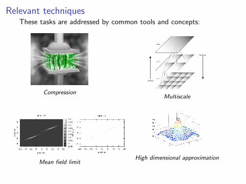
Relevant techniquesThese tasks are addressed by common tools and concepts:
Compression
Mean field limit
Multiscale
High dimensional approximation
MODELING, SIMULATION, LEARNING, CONTROL

Relevant techniquesThese tasks are addressed by common tools and concepts:
Compression
Mean field limit
Multiscale
High dimensional approximation
MODELING, SIMULATION, LEARNING, CONTROL

Compression
“–Compression can be mathematically expressed as - numerically -approximating a certain function, sometimes explicitely given or, asmore often, only implicitly given as a solution of a certain equationor variational problem, by using the minimal/optimal amount ofdegrees of freedom.–”

Social dynamics
We consider Dynamical Systems ofmutual distances Dx = (‖xi − xj‖)ij :
xi (t) = fi (Dx(t))+N∑
j=1
fij(Dx(t))xj(t).
Several“social forces” encoded in fiand fij :
I Repulsion-attraction
I Self-drive
I Noise/uncertainty
I ...
Patterns related to different balance of
social forces.
Understanding how superposition of re-iterated binary “socialforces” yields global self-organization.

An example inspired by nature
Mills in nature and in our simulations.
J. A. Carrillo, M. Fornasier, G. Toscani, and F. Vecil, Particle, kinetic,
hydrodynamic models of swarming, within the book “Mathematical modeling
of collective behavior in socio-economic and life-sciences”, Birkhauser (Eds.
Lorenzo Pareschi, Giovanni Naldi, and Giuseppe Toscani), 2010.

Consensus emergenceThe Cucker-Smale model:
xi = vi ∈ Rd
vi =1
N
N∑j=1
a(‖xj − xi‖)(vj − vi ) ∈ Rd,
where a(t) := aβ(t) = 1(1+t2)β
, β > 0 governs the rate of
communication.
In matrix notation:{x = v
v = −Lxv
where Lx is the Laplacian of the matrix1 (a(‖xj − xi‖)/N)Ni ,j=1
and depends on x .
I Mean-velocity conservation:ddt v(t) = 1
N
∑Ni=1 vi (t) = 1
N2
∑Ni=1
∑Nj=1
vj−vi
(1+‖xj−xi‖2)β≡ 0.
1The Laplacian L of A is given by L = D − A, with D = diag(d1, . . . , dN)and dk =
PNj=1 akj

Consensus emergenceThe Cucker-Smale model:
xi = vi ∈ Rd
vi =1
N
N∑j=1
a(‖xj − xi‖)(vj − vi ) ∈ Rd,
where a(t) := aβ(t) = 1(1+t2)β
, β > 0 governs the rate of
communication. In matrix notation:{x = v
v = −Lxv
where Lx is the Laplacian of the matrix1 (a(‖xj − xi‖)/N)Ni ,j=1
and depends on x .
I Mean-velocity conservation:ddt v(t) = 1
N
∑Ni=1 vi (t) = 1
N2
∑Ni=1
∑Nj=1
vj−vi
(1+‖xj−xi‖2)β≡ 0.
1The Laplacian L of A is given by L = D − A, with D = diag(d1, . . . , dN)and dk =
PNj=1 akj

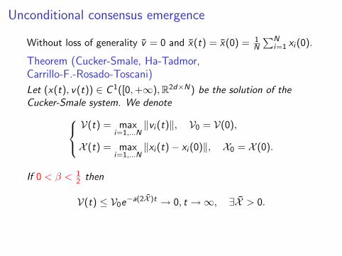
Unconditional consensus emergence
Without loss of generality v = 0 and x(t) = x(0) = 1N
∑Ni=1 xi (0).
Theorem (Cucker-Smale, Ha-Tadmor,Carrillo-F.-Rosado-Toscani)
Let (x(t), v(t)) ∈ C 1([0,+∞),R2d×N) be the solution of theCucker-Smale system. We denote
V(t) = maxi=1,...N
‖vi (t)‖, V0 = V(0),
X (t) = maxi=1,...N
‖xi (t)− xi (0)‖, X0 = X (0).
If 0 < β < 12 then
V(t) ≤ V0e−a(2X )t → 0, t →∞, ∃X > 0.
Actually one has V(t)→ 0 also for β = 1/2.

Conditional consensus emergence for a genericcommunication rate a(·)
Consider the symmetric bilinear form
B(u, v) =1
2N2
∑i ,j
〈ui − uj , vi − vj〉 =1
N
N∑i=1
〈ui , vi 〉 − 〈u, v〉,
andX (t) = B(x(t), x(t)), V (t) = B(v(t), v(t)).
Theorem (Ha-Ha-Kim)
Let (x0, v0) ∈ (Rd)N × (Rd)N be such thatX0 = B(x0, x0) and V0 = B(v0, v0) satisfy
√N
∫ ∞√
NX0
a(√
2r)dr >√
V0 .
Then the solution with initial data (x0, v0)tends to consensus.

Non-consensus eventsIf β > 1/2 then for a(·) = aβ(·) the consensus condition is notsatisfied by all (x0, v0) ∈ (Rd)N × (Rd)N .There are counterexamples to consensus emergence(Caponigro-F.-Piccoli-Trelat).
Consider β = 1 and x(t) = x1(t)− x2(t), v(t) = v1(t)− v2(t)relative pos. and vel. of two agents on the line: x = v
v = − v
1 + x2
with initial conditions x(0) = x0 and v(0) = v0 > 0.By direct integration
v(t) = − arctan x(t) + arctan x0 + v0.
Hence, if arctan x0 + v0 > π/2 + ε we have
v(t) > π/2 + ε− arctan x(t) > ε, ∀t ∈ R+.

Non-consensus eventsIf β > 1/2 then for a(·) = aβ(·) the consensus condition is notsatisfied by all (x0, v0) ∈ (Rd)N × (Rd)N .There are counterexamples to consensus emergence(Caponigro-F.-Piccoli-Trelat).Consider β = 1 and x(t) = x1(t)− x2(t), v(t) = v1(t)− v2(t)relative pos. and vel. of two agents on the line: x = v
v = − v
1 + x2
with initial conditions x(0) = x0 and v(0) = v0 > 0.
By direct integration
v(t) = − arctan x(t) + arctan x0 + v0.
Hence, if arctan x0 + v0 > π/2 + ε we have
v(t) > π/2 + ε− arctan x(t) > ε, ∀t ∈ R+.

Non-consensus eventsIf β > 1/2 then for a(·) = aβ(·) the consensus condition is notsatisfied by all (x0, v0) ∈ (Rd)N × (Rd)N .There are counterexamples to consensus emergence(Caponigro-F.-Piccoli-Trelat).Consider β = 1 and x(t) = x1(t)− x2(t), v(t) = v1(t)− v2(t)relative pos. and vel. of two agents on the line: x = v
v = − v
1 + x2
with initial conditions x(0) = x0 and v(0) = v0 > 0.By direct integration
v(t) = − arctan x(t) + arctan x0 + v0.
Hence, if arctan x0 + v0 > π/2 + ε we have
v(t) > π/2 + ε− arctan x(t) > ε, ∀t ∈ R+.

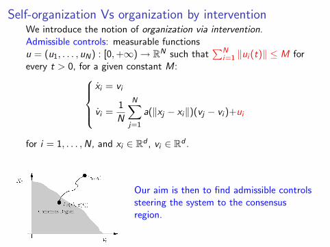
Self-organization Vs organization by interventionWe introduce the notion of organization via intervention.
Admissible controls: measurable functionsu = (u1, . . . , uN) : [0,+∞)→ RN such that
∑Ni=1 ‖ui (t)‖ ≤ M for
every t > 0, for a given constant M:xi = vi
vi =1
N
N∑j=1
a(‖xj − xi‖)(vj − vi )+ui
for i = 1, . . . ,N, and xi ∈ Rd , vi ∈ Rd .
Our aim is then to find admissible controlssteering the system to the consensusregion.

Self-organization Vs organization by interventionWe introduce the notion of organization via intervention.Admissible controls: measurable functionsu = (u1, . . . , uN) : [0,+∞)→ RN such that
∑Ni=1 ‖ui (t)‖ ≤ M for
every t > 0, for a given constant M:xi = vi
vi =1
N
N∑j=1
a(‖xj − xi‖)(vj − vi )+ui
for i = 1, . . . ,N, and xi ∈ Rd , vi ∈ Rd .
Our aim is then to find admissible controlssteering the system to the consensusregion.

Total control
Proposition (Caponigro-F.-Piccoli-Trelat)
For every initial condition (x0, v0) ∈ (Rd)N × (Rd)N and M > 0there exist T > 0 and u : [0,T ]→ (Rd)N , with
∑Ni=1 ‖ui (t)‖ ≤ M
for every t ∈ [0,T ] such that the associated solution tends toconsensus.
Proof.Consider a solution of system with initial data (x0, v0) associatedwith a feedback control u = −α(v − v), with0 < α ≤ M/(N
√B(v0, v0)). Then
d
dtV (t) =
d
dtB(v(t), v(t))
= −2B(Lxv(t), v(t)) + 2B(u(t), v(t))
≤ 2B(u(t), v(t)) = −2αB(v − v , v − v) = −2αV (t).
Therefore V (t) ≤ e−2αtV (0) and V (t) tends to 0 exponentiallyfast as t →∞. Moreover
∑Ni=1 ‖ui‖ ≤ M.

Total control
Proposition (Caponigro-F.-Piccoli-Trelat)
For every initial condition (x0, v0) ∈ (Rd)N × (Rd)N and M > 0there exist T > 0 and u : [0,T ]→ (Rd)N , with
∑Ni=1 ‖ui (t)‖ ≤ M
for every t ∈ [0,T ] such that the associated solution tends toconsensus.
Proof.Consider a solution of system with initial data (x0, v0) associatedwith a feedback control u = −α(v − v), with0 < α ≤ M/(N
√B(v0, v0)).
Then
d
dtV (t) =
d
dtB(v(t), v(t))
= −2B(Lxv(t), v(t)) + 2B(u(t), v(t))
≤ 2B(u(t), v(t)) = −2αB(v − v , v − v) = −2αV (t).
Therefore V (t) ≤ e−2αtV (0) and V (t) tends to 0 exponentiallyfast as t →∞. Moreover
∑Ni=1 ‖ui‖ ≤ M.

Total control
Proposition (Caponigro-F.-Piccoli-Trelat)
For every initial condition (x0, v0) ∈ (Rd)N × (Rd)N and M > 0there exist T > 0 and u : [0,T ]→ (Rd)N , with
∑Ni=1 ‖ui (t)‖ ≤ M
for every t ∈ [0,T ] such that the associated solution tends toconsensus.
Proof.Consider a solution of system with initial data (x0, v0) associatedwith a feedback control u = −α(v − v), with0 < α ≤ M/(N
√B(v0, v0)). Then
d
dtV (t) =
d
dtB(v(t), v(t))
= −2B(Lxv(t), v(t)) + 2B(u(t), v(t))
≤ 2B(u(t), v(t)) = −2αB(v − v , v − v) = −2αV (t).
Therefore V (t) ≤ e−2αtV (0) and V (t) tends to 0 exponentiallyfast as t →∞. Moreover
∑Ni=1 ‖ui‖ ≤ M.

Total control
Proposition (Caponigro-F.-Piccoli-Trelat)
For every initial condition (x0, v0) ∈ (Rd)N × (Rd)N and M > 0there exist T > 0 and u : [0,T ]→ (Rd)N , with
∑Ni=1 ‖ui (t)‖ ≤ M
for every t ∈ [0,T ] such that the associated solution tends toconsensus.
Proof.Consider a solution of system with initial data (x0, v0) associatedwith a feedback control u = −α(v − v), with0 < α ≤ M/(N
√B(v0, v0)). Then
d
dtV (t) =
d
dtB(v(t), v(t))
= −2B(Lxv(t), v(t)) + 2B(u(t), v(t))
≤ 2B(u(t), v(t)) = −2αB(v − v , v − v) = −2αV (t).
Therefore V (t) ≤ e−2αtV (0) and V (t) tends to 0 exponentiallyfast as t →∞. Moreover
∑Ni=1 ‖ui‖ ≤ M.

More economical choices?
We wish to make
d
dtV (t) =
d
dtB(v(t), v(t))
= −2B(Lxv(t), v(t)) + 2B(u(t), v(t))
the smallest possible and use the minimal amount of intervention:
minimize B(u(t), v(t)) with additional sparsity constraints.

More economical choices?
We wish to make
d
dtV (t) =
d
dtB(v(t), v(t))
= −2B(Lxv(t), v(t)) + 2B(u(t), v(t))
the smallest possible and use the minimal amount of intervention:minimize B(u(t), v(t)) with additional sparsity constraints.

Linear dynamical systems
Were the dependence of the trajectory(x(t), v(t)) at the time t on the controlu := {u(s) : s ∈ [0, t]} linear
(x(t), v(t)) = Mx0,v0,tu,
then a rather general theory of linearcompression would apply.

Compressed sensing enters the picture
TheoremGiven a matrix M ∈ Rk×d , k � d, with incoherency propertiesMT M ≈ I , and
x = Mu + e ∈ Rk , ‖e‖ ≤ ε,
the vector u computed by
u = arg min‖Mv−x‖≤ε
‖v‖`1 :=d∑
i=1
|vi |, (`1)
has the approximation property
‖u − u‖ ≤ C1σK (u)1√
K+ C2ε,
where σK (v)1 = ‖v − v[K ]‖`1 , best-K -term approx. error. If u issparse then σK (u)1 = 0.

Geometrical interpretation
Minimal `1-norm solution.
Assume d = 2 and k = 1.Hence F(x) = {z : Mu = x} isjust a line in R2. If we excludethat there exists η ∈ ker Msuch that |η1| = |η2| or,equivalently,
|ηi | < |η{1,2}\{i}|
for all η ∈ ker M and for onei = 1, 2, then the solution to(`1) is a sparse solution.
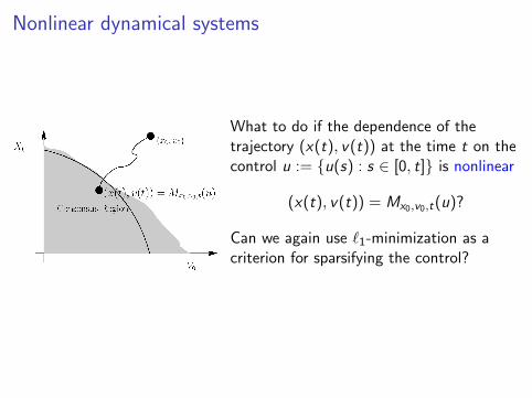
Nonlinear dynamical systems
What to do if the dependence of thetrajectory (x(t), v(t)) at the time t on thecontrol u := {u(s) : s ∈ [0, t]} is nonlinear
(x(t), v(t)) = Mx0,v0,t(u)?
Can we again use `1-minimization as acriterion for sparsifying the control?

Greedy sparse control
Theorem (Caponigro-F.-Piccoli-Trelat)
For every initial condition (x0, v0) ∈ (Rd)N × (Rd)N and M > 0there exist T > 0 and a sparse control u : [0,T ]→ (Rd)N , with∑N
i=1 ‖ui (t)‖ ≤ M for every t ∈ [0,T ] such that the associated ACsolution tends to consensus.
More precisely, we can chooseadaptively the control law explicitly as one of the solutions of thevariational problem
min B(v , u) +γ(x)
N
N∑i=1
‖ui‖ subject toN∑
i=1
‖ui‖ ≤ M ,
where
γ(x) =√
N
∫ ∞√
NB(x ,x)a(√
2r)dr .
The control u(t) is a sparse vector with at most one nonzerocoordinate, i.e., ui (t) 6= 0 for a unique i ∈ {1, . . . ,N} anduj(t) = 0 for j 6= i for almost every t ∈ [0,T ].

Greedy sparse control
Theorem (Caponigro-F.-Piccoli-Trelat)
For every initial condition (x0, v0) ∈ (Rd)N × (Rd)N and M > 0there exist T > 0 and a sparse control u : [0,T ]→ (Rd)N , with∑N
i=1 ‖ui (t)‖ ≤ M for every t ∈ [0,T ] such that the associated ACsolution tends to consensus. More precisely, we can chooseadaptively the control law explicitly as one of the solutions of thevariational problem
min B(v , u) +γ(x)
N
N∑i=1
‖ui‖ subject toN∑
i=1
‖ui‖ ≤ M ,
where
γ(x) =√
N
∫ ∞√
NB(x ,x)a(√
2r)dr .
The control u(t) is a sparse vector with at most one nonzerocoordinate, i.e., ui (t) 6= 0 for a unique i ∈ {1, . . . ,N} anduj(t) = 0 for j 6= i for almost every t ∈ [0,T ].

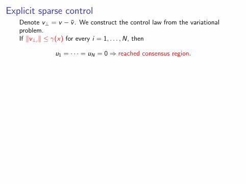
Explicit sparse controlDenote v⊥ = v − v . We construct the control law from the variationalproblem.
If ‖v⊥i‖ ≤ γ(x) for every i = 1, . . . ,N, then
u1 = · · · = uN = 0⇒ reached consensus region.
Otherwise there exists a “best index” i ∈ {1, . . . ,N} such that
‖v⊥i‖ > γ(x) and ‖v⊥i‖ ≥ ‖v⊥j‖ for every j = 1, . . . ,N.
Therefore we can choose i ∈ {1, . . . ,N} satisfying it, and a control law
ui = −Mv⊥i
‖v⊥i‖, and uj = 0, for every j 6= i .
Hence the control acts on the most“stubborn”. We may call this control the“shepherd dog strategy”. This choice of thecontrol makes V (t) = B(v(t), v(t)) vanishingin finite time, hence there exists T such thatB(v(t), v(t)) ≤ γ(x)2, t ≥ T .

Explicit sparse controlDenote v⊥ = v − v . We construct the control law from the variationalproblem.If ‖v⊥i‖ ≤ γ(x) for every i = 1, . . . ,N, then
u1 = · · · = uN = 0
⇒ reached consensus region.
Otherwise there exists a “best index” i ∈ {1, . . . ,N} such that
‖v⊥i‖ > γ(x) and ‖v⊥i‖ ≥ ‖v⊥j‖ for every j = 1, . . . ,N.
Therefore we can choose i ∈ {1, . . . ,N} satisfying it, and a control law
ui = −Mv⊥i
‖v⊥i‖, and uj = 0, for every j 6= i .
Hence the control acts on the most“stubborn”. We may call this control the“shepherd dog strategy”. This choice of thecontrol makes V (t) = B(v(t), v(t)) vanishingin finite time, hence there exists T such thatB(v(t), v(t)) ≤ γ(x)2, t ≥ T .
Explicit sparse controlDenote v⊥ = v − v . We construct the control law from the variationalproblem.If ‖v⊥i‖ ≤ γ(x) for every i = 1, . . . ,N, then
u1 = · · · = uN = 0⇒ reached consensus region.
Otherwise there exists a “best index” i ∈ {1, . . . ,N} such that
‖v⊥i‖ > γ(x) and ‖v⊥i‖ ≥ ‖v⊥j‖ for every j = 1, . . . ,N.
Therefore we can choose i ∈ {1, . . . ,N} satisfying it, and a control law
ui = −Mv⊥i
‖v⊥i‖, and uj = 0, for every j 6= i .
Hence the control acts on the most“stubborn”. We may call this control the“shepherd dog strategy”. This choice of thecontrol makes V (t) = B(v(t), v(t)) vanishingin finite time, hence there exists T such thatB(v(t), v(t)) ≤ γ(x)2, t ≥ T .

Explicit sparse controlDenote v⊥ = v − v . We construct the control law from the variationalproblem.If ‖v⊥i‖ ≤ γ(x) for every i = 1, . . . ,N, then
u1 = · · · = uN = 0⇒ reached consensus region.
Otherwise there exists a “best index” i ∈ {1, . . . ,N} such that
‖v⊥i‖ > γ(x) and ‖v⊥i‖ ≥ ‖v⊥j‖ for every j = 1, . . . ,N.
Therefore we can choose i ∈ {1, . . . ,N} satisfying it, and a control law
ui = −Mv⊥i
‖v⊥i‖, and uj = 0, for every j 6= i .
Hence the control acts on the most“stubborn”. We may call this control the“shepherd dog strategy”.
This choice of thecontrol makes V (t) = B(v(t), v(t)) vanishingin finite time, hence there exists T such thatB(v(t), v(t)) ≤ γ(x)2, t ≥ T .

Explicit sparse controlDenote v⊥ = v − v . We construct the control law from the variationalproblem.If ‖v⊥i‖ ≤ γ(x) for every i = 1, . . . ,N, then
u1 = · · · = uN = 0⇒ reached consensus region.
Otherwise there exists a “best index” i ∈ {1, . . . ,N} such that
‖v⊥i‖ > γ(x) and ‖v⊥i‖ ≥ ‖v⊥j‖ for every j = 1, . . . ,N.
Therefore we can choose i ∈ {1, . . . ,N} satisfying it, and a control law
ui = −Mv⊥i
‖v⊥i‖, and uj = 0, for every j 6= i .
Hence the control acts on the most“stubborn”. We may call this control the“shepherd dog strategy”. This choice of thecontrol makes V (t) = B(v(t), v(t)) vanishingin finite time, hence there exists T such thatB(v(t), v(t)) ≤ γ(x)2, t ≥ T .

Geometrical interpretation in the scalar case
For |v | ≤ γ the minimal solution u ∈ [−M,M] is zero.
For |v | > γ the minimal solution u ∈ [−M,M] is |u| = M.

Instantaneous optimality of the greedy strategy
Consider generic control u (solution of the variation problem) ofcomponents
ui (x , v) =
0 if v⊥i
= 0
− αiv⊥i
‖v⊥i‖
if v⊥i6= 0
where αi ≥ 0 such that∑N
i=1 αi ≤ M.
Theorem (Caponigro-F.-Piccoli-Trelat)
The 1-sparse control isthe minimizer of
R(t, u) := R(t) =d
dtV (t),
among all the control ofthe previous form.
A policy maker, who is not allowed to haveprediction on future developments, shouldalways consider more favorable to intervenewith stronger actions on the fewest possibleinstantaneous optimal leaders than trying tocontrol more agents with minor strength.

Time-sparse control: sampling-and-hold
Definition (Sampling solution)
Let U ⊂ Rm, f : Rn × U 7→ f (x , u) be continuous and locallyLipschitz in x uniformly on compact subset of Rn × U. Given afeedback u : Rn → U, τ > 0, and x0 ∈ Rn we define the samplingsolution of
x = f (x , u(x)), x(0) = x0
as the continuous (actually piecewise C 1) function x : [0,T ]→ Rn
solving recursively for k ≥ 0
x(t) = f (x(t), u(x(kτ))), t ∈ [kτ, (k + 1)τ ]
using as initial value x(kτ) the endpoint of the solution on thepreceding interval and starting with x(0) = x0.

Time-sparse control: sampling-and-holdWe define u = u(x , v) via the following criterion. IfB(v , v) ≥ γ(B(x , x))2 then let i ∈ {1, . . . ,N} be the smallestindex such that
‖v⊥i‖ ≥ γ(B(x , x)) and ‖v⊥i
‖ ≥ ‖v⊥j‖ for every j = 1, . . . ,N.
and set
ui = −Mv⊥i
‖v⊥i‖, and uj = 0, for every j 6= i ,
Theorem (Caponigro-F.-Piccoli-Trelat)
For every initial condition (x0, v0) ∈ (Rd)N × (Rd)N and M > 0consider the control u given above. There existsτ0 = τ0(M,N, x0, v0) > 0 small enough, such that for all0 < τ ≤ τ0 the sampling solution associated with the control u,the sampling time τ , and initial datum (x0, v0) tends to consensus
in time T ≤ N2M (
√V (0)− γ(X )), X = 2B(x0, x0) + 2N4
M2 B(v0, v0)2.

Complexty of consensusGiven a stuitable compact set K ⊂ (Rd)N × (Rd)N of initialconditions, control bound M > 0, number of agents N ∈ N, andarrival time T > 0, we define
n := n(M,N,K,T )
= inf sup(x0,v0)∈K
{k−1∑`=0
# supp(u(t`)) :
(x(T ; u), v(T , u)) is in the consensus region }
The previous result allow us to have upper bounds for thisconsensus numbers: for
T = T (M,N, x0, v0) =N
2M(√
V (0)− γ(X )),
n(M,N,K,T ) ≤
{∞, T < Tsup(x0,v0)∈K T (M,N,x0,v0)
inf(x0,v0)∈K τ0(M,N,x0,v0) , T ≥ T
Presently lower bounds are not yet given.

Complexty of consensusGiven a stuitable compact set K ⊂ (Rd)N × (Rd)N of initialconditions, control bound M > 0, number of agents N ∈ N, andarrival time T > 0, we define
n := n(M,N,K,T )
= inf sup(x0,v0)∈K
{k−1∑`=0
# supp(u(t`)) :
(x(T ; u), v(T , u)) is in the consensus region }
The previous result allow us to have upper bounds for thisconsensus numbers:
for
T = T (M,N, x0, v0) =N
2M(√
V (0)− γ(X )),
n(M,N,K,T ) ≤
{∞, T < Tsup(x0,v0)∈K T (M,N,x0,v0)
inf(x0,v0)∈K τ0(M,N,x0,v0) , T ≥ T
Presently lower bounds are not yet given.

Complexty of consensusGiven a stuitable compact set K ⊂ (Rd)N × (Rd)N of initialconditions, control bound M > 0, number of agents N ∈ N, andarrival time T > 0, we define
n := n(M,N,K,T )
= inf sup(x0,v0)∈K
{k−1∑`=0
# supp(u(t`)) :
(x(T ; u), v(T , u)) is in the consensus region }
The previous result allow us to have upper bounds for thisconsensus numbers: for
T = T (M,N, x0, v0) =N
2M(√
V (0)− γ(X )),
n(M,N,K,T ) ≤
{∞, T < Tsup(x0,v0)∈K T (M,N,x0,v0)
inf(x0,v0)∈K τ0(M,N,x0,v0) , T ≥ T
Presently lower bounds are not yet given.

Complexty of consensusGiven a stuitable compact set K ⊂ (Rd)N × (Rd)N of initialconditions, control bound M > 0, number of agents N ∈ N, andarrival time T > 0, we define
n := n(M,N,K,T )
= inf sup(x0,v0)∈K
{k−1∑`=0
# supp(u(t`)) :
(x(T ; u), v(T , u)) is in the consensus region }
The previous result allow us to have upper bounds for thisconsensus numbers: for
T = T (M,N, x0, v0) =N
2M(√
V (0)− γ(X )),
n(M,N,K,T ) ≤
{∞, T < Tsup(x0,v0)∈K T (M,N,x0,v0)
inf(x0,v0)∈K τ0(M,N,x0,v0) , T ≥ T
Presently lower bounds are not yet given.
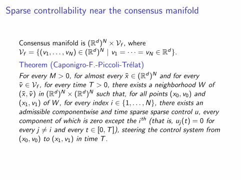
Sparse controllability near the consensus manifold
Consensus manifold is (Rd)N × Vf , whereVf = {(v1, . . . , vN) ∈ (Rd)N | v1 = · · · = vN ∈ Rd}.
Theorem (Caponigro-F.-Piccoli-Trelat)
For every M > 0, for almost every x ∈ (Rd)N and for everyv ∈ Vf , for every time T > 0, there exists a neighborhood W of(x , v) in (Rd)N × (Rd)N such that, for all points (x0, v0) and(x1, v1) of W , for every index i ∈ {1, . . . ,N}, there exists anadmissible componentwise and time sparse sparse control u, everycomponent of which is zero except the i th (that is, uj(t) = 0 forevery j 6= i and every t ∈ [0,T ]), steering the control system from(x0, v0) to (x1, v1) in time T .

Global sparse controllability
Corollary (Caponigro-F.-Piccoli-Trelat)
For every M > 0, for every initial condition(x0, v0) ∈ (Rd)N × (Rd)N , for almost every (x1, v1) ∈ (Rd)N × Vf ,there exist T > 0 and an admissible componentwise and timesparse control u : [0,T ]→ (Rd)N , such that the correspondingsolution starting at (x0, v0) arrives at the consensus point (x1, v1)within time T .

Sparse optimal control
The problem is to minimize, for a given γ > 0
J (u) :=
∫ T
0
N∑i=1
((vi (t)− 1
N
N∑j=1
vj(t))2
+ γ
N∑i=1
‖ui (t)‖)
dt,
s.t.∑‖ui‖ ≤ M
where the state is a trajectory of the control systemxi = vi
vi =1
N
N∑j=1
a(‖xj − xi‖)(vj − vi ) + ui
with initial constraint
(x(0), v(0)) = (x0, v0) ∈ (Rd)N × (Rd)N .

Beyond a greedy approach: sparse optimal control
Theorem (Caponigro-F.-Piccoli-Trelat)
For every (x0, v0) in (Rd)N × (Rd)N , for every M > 0, and forevery γ > 0 the optimal control problem has an optimal solution.The optimal control u(t) is “usually” instantaneously a vector withat most one nonzero coordinate.
The PMP ensures the existence of λ ≥ 0 and of a nontrivialcovector (px , pv ) ∈ (Rd)N × (Rd)N satisfying the adjointequations, for i = 1, . . . ,N,
pxi =1
N
N∑j=1
a(‖xj − xi‖)‖xj − xi‖
〈xj − xi , vj − vi 〉(pvj − pvi )
pvi = −pxi −1
N
∑j 6=i
a(‖xj − xi‖)(pvj − pvi )− 2λvi +2λ
N
N∑j=1
vj .
The application of the PMP leads to minimize
minN∑
i=1
〈pvi , ui 〉+ λγN∑
i=1
‖ui‖, subject toN∑
i=1
‖ui‖ ≤ M.

Beyond a greedy approach: sparse optimal control
Theorem (Caponigro-F.-Piccoli-Trelat)
For every (x0, v0) in (Rd)N × (Rd)N , for every M > 0, and forevery γ > 0 the optimal control problem has an optimal solution.The optimal control u(t) is “usually” instantaneously a vector withat most one nonzero coordinate.
The PMP ensures the existence of λ ≥ 0 and of a nontrivialcovector (px , pv ) ∈ (Rd)N × (Rd)N satisfying the adjointequations, for i = 1, . . . ,N,
pxi =1
N
N∑j=1
a(‖xj − xi‖)‖xj − xi‖
〈xj − xi , vj − vi 〉(pvj − pvi )
pvi = −pxi −1
N
∑j 6=i
a(‖xj − xi‖)(pvj − pvi )− 2λvi +2λ
N
N∑j=1
vj .
The application of the PMP leads to minimize
minN∑
i=1
〈pvi , ui 〉+ λγ
N∑i=1
‖ui‖, subject toN∑
i=1
‖ui‖ ≤ M.

Conclusion
I We presented dynamical systems withself-organization features.
I In case pattern formation cannot beensured, we introduced the concept oforganization by external intervention.
I We proved that the most effectivegreedy strategy to achieve consensusemergence is by instantaneous1-sparse controls.
I We showed that maximally sparseoptimal control are also expectedwhen considering `1-norm constraints.

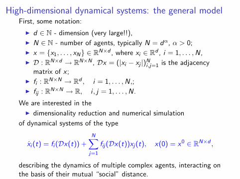
High-dimensional dynamical systems: the general modelFirst, some notation:
I d ∈ N - dimension (very large!!),
I N ∈ N - number of agents, typically N = dα, α > 0;
I x = {x1, . . . , xN} ∈ RN×d , where xi ∈ Rd , i = 1, . . . ,N,
I D : RN×d → RN×N , Dx = (|xi − xj |)Ni ,j=1 is the adjacency
matrix of x ;
I fi : RN×N → Rd , i = 1, . . . ,N,;
I fij : RN×N → R, i , j = 1, . . . ,N.
We are interested in the
I dimensionality reduction and numerical simulation
of dynamical systems of the type
xi (t) = fi (Dx(t)) +N∑
j=1
fij(Dx(t))xj(t), x(0) = x0 ∈ RN×d ,
describing the dynamics of multiple complex agents, interacting onthe basis of their mutual “social” distance.

The application framework
With the development of communication technology and Internet,larger and larger groups of people will access
I information (interactive database access, trends in scientificliterature and in newspapers ...)
I services (Google, the financial market ...)
I social interactions (social networks ...)
Our aim is to provide innovative tools for analyzing, simulating,even predicting and controlling the behavior of such large crowds,as one today can already do with weather forecasts.
We are facing very difficult challenges due to the “curse ofdimensionality”, as our individuals are not physical particles andneed a large number d of degrees of freedom to be described.

Relevant assumptions
We assume the following Lipschitz and boundedness properties offi and fij , namely
‖fi (a)− fi (b)‖ ≤ L‖a− b‖∞,
maxi
∑j
|fij(a)| ≤ L′,
maxi
∑j
|fij(a)− fij(b)| ≤ L′′‖a− b‖∞,
for every a, b ∈ RN×N . Here, ‖a− b‖∞ := maxi ,j |aij − bij |.
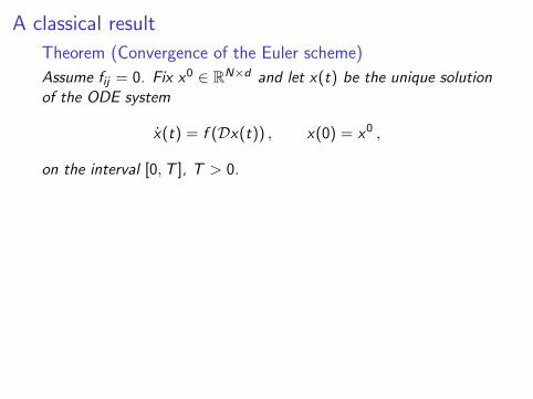
A classical result
Theorem (Convergence of the Euler scheme)
Assume fij = 0. Fix x0 ∈ RN×d and let x(t) be the unique solutionof the ODE system
x(t) = f (Dx(t)) , x(0) = x0 ,
on the interval [0,T ], T > 0.
Fix h > 0 and tn := nh:
xn+1 = xn + hf (Dxn) , x0 = x0 ,
for n = 1, 2, . . . .
Then, we have the estimate for en = ‖x(tn)− xn‖,
en ≤ exp(Ltn)
(e0 + htn
‖f (Dx0)‖2
).

Exponential complexity reduction in d
The complexity of this algorithm stems from the evaluation off (Dx) which can be (generically) estimated by
O(d × N2).
Our first aim is to find an appropriate model of appropriatereduction of the dynamical system to log(d) dimensions andconsequently the complexity to
O(log(d)× N2).

Dimensionality reduction via Johnson-Lindenstraussembeddings
Again some notation
I ε > 0 - a distortion parameter from J-L Lemma, see below,
I n0 ∈ N - number of iterations,
I N = n0N - number of iterations times number of agents
I k = O(ε−2 log(N )), new lower dimension - see below,
I M ∈ Rk×d - randomly generated matrix, see below,
I D : RN×d → RN×N , Dx = (‖xi − xj‖)Ni ,j=1 is the adjacency
matrix in high-dimension and similarly definedD′ : RN×k → RN×N , D′y = (‖yi − yj‖)N
i ,j=1, the one inlow-dimension.

Dimensionality reduction via Johnson-Lindenstraussembeddings
Lemma (Johnson and Lindenstrauss)
Let P be an arbitrary set of N points in Rd . Given ε > 0, thereexists
k0 = O(ε−2 log(N )),
such that for all integers k ≥ k0, there exists a k × d randommatrix M for which with high probability, for all x , x ∈ P
(1− ε)‖x − x‖2 ≤ ‖Mx −Mx‖2 ≤ (1 + ε)‖x − x‖2.

Dimensionality reduction via Johnson-Lindenstraussembeddings

Restricted Isometry Property
DefinitionA k × d matrix M is said to have the Restricted Isometry Propertyof order K ≤ d and level δ ∈ (0, 1) if
(1− δ)‖x‖2 ≤ ‖Mx‖2 ≤ (1 + δ)‖x‖2
for all K -sparse x ∈ Rd , i.e., # supp(x) ≤ K .
Theorem (Krahmer, Ward)
Fix η > 0 and ε > 0, and consider a finite set P ⊂ Rd of cardinality|P| = N . Set K ≥ 40 log 4N
η , and suppose that the k × d matrix
M satisfies the Restricted Isometry Property of order K and levelδ ≤ ε/4. Let ξ ∈ Rd be a Rademacher sequence, i.e., uniformlydistributed on {−1, 1}d . Then with probability exceeding 1− η,
(1− ε)‖x‖2 ≤ ‖Mx‖2 ≤ (1 + ε)‖x‖2.
uniformly for all x ∈ P, where M := M diag(ξ).

Some stochastic constructions of RIP→JL matricesThe following matrices satisfies the RIP w.h.p. for
K = O(
k
1 + log(d/k)
).
I k × d matrices M whose entries mi,j are independent realizations ofGaussian random variables
mi,j ∼ N(
0,1
k
);
I k × d matrices M whose entries are independent realizations of ±Bernoulli random variables
mi,j :=
{+ 1√
k, with probability 1
2
− 1√k, with probability 1
2
More matrices: by random sampling of bounded basis (e.g., Fourierbasis) or random circulant matrices.

Projection of the dynamical systemWe consider the system of ordinary differential equations in thefixed form with the initial condition
xi (0) = x0i , i = 1, . . . ,N .
The Euler method for this system is given by this initial conditionand
xn+1i := xn
i + h
fi (Dxn) +N∑
j=1
fij(Dxn)xnj
, n = 0, . . . , n0 − 1.
where h > 0 is the time step and n0 := T/h is the number ofiterations.
If M ∈ Rk×d is a matrix, we may consider the associated Eulermethod in Rk , namely
y 0i := Mx0
i ,
yn+1i := yn
i + h
Mfi (D′yn) +N∑
j=1
fij(D′yn)ynj
, n = 0, . . . , n0 − 1.

Projection of the dynamical systemWe consider the system of ordinary differential equations in thefixed form with the initial condition
xi (0) = x0i , i = 1, . . . ,N .
The Euler method for this system is given by this initial conditionand
xn+1i := xn
i + h
fi (Dxn) +N∑
j=1
fij(Dxn)xnj
, n = 0, . . . , n0 − 1.
where h > 0 is the time step and n0 := T/h is the number ofiterations.If M ∈ Rk×d is a matrix, we may consider the associated Eulermethod in Rk , namely
y 0i := Mx0
i ,
yn+1i := yn
i + h
Mfi (D′yn) +N∑
j=1
fij(D′yn)ynj
, n = 0, . . . , n0 − 1.

A first surprising result
Theorem (Fornasier, Haskovec, Vybıral)
Given a matrix M ∈ Rk×d such that∥∥Mfi (D′yn)−Mfi (Dxn)∥∥ ≤ (1 + ε)
∥∥fi (D′yn)− fi (Dxn)∥∥ ,
‖Mxnj ‖ ≤ (1 + ε)‖xn
j ‖,(1− ε)‖xn
i − xnj ‖ ≤ ‖Mxn
i −Mxnj ‖ ≤ (1 + ε)‖xn
i − xnj ‖
for all i , j = 1, . . . ,N and all n = 0, . . . , n0. Let us also assume,that α ≥ maxj ‖xn
j ‖ for all n = 0, . . . , n0, j = 1, . . . ,N. Let
eni := ‖yn
i −Mxni ‖, i = 1, . . . ,N and n = 0, . . . , n0
and put En := maxi eni . Then
En ≤ εhnB exp(hnA),
where A := L′ + 2(1 + ε)(L + αL′′) and B := 2α(1 + ε)(L + αL′′).

Visual explanation
A continuous Johnson-Lindenstrauss Lemma
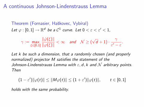
Theorem (Fornasier, Haskovec, Vybıral)
Let ϕ : [0, 1]→ Rd be a C1 curve. Let 0 < ε < ε′ < 1,
γ := maxξ∈[0,1]
‖ϕ(ξ)‖‖ϕ(ξ)‖
<∞ and N ≥ (√
d + 1) · γ
ε′ − ε.
Let k be such a dimension, that a randomly chosen (and properlynormalized) projector M satisfies the statement of theJohnson-Lindenstrauss Lemma with ε, d , k and N arbitrary points.Then
(1− ε′)‖ϕ(t)‖ ≤ ‖Mϕ(t)‖ ≤ (1 + ε′)‖ϕ(t)‖, t ∈ [0, 1]
holds with the same probability.

A continuous Johnson-Lindenstrauss Lemma
The condition
γ := maxξ∈[0,1]
‖ϕ(ξ)‖‖ϕ(ξ)‖
<∞ and N ≥ (√
d + 1) · γ
ε′ − ε
is necessary.y
Peano’s space-filling curve
By lifting a suitable parametrizationa Peano’s space-filling curve on theunit sphere Sd−1, one generates acurve with infinite speed (i.e., thecondition does not hold), and at thesame time it generates any possiblevector including those in the kernelof M, hence
(1− ε′)‖ϕ(t)‖ ≤ ‖Mϕ(t)‖
cannot hold!

Projecting the continuous system
Theorem (Fornasier, Haskovec, Vybıral)
Let x(t) ∈ Rd×N , t ∈ [0,T ], be the solution of the given ODEsystem, such that maxt∈[0,T ] maxi ,j ‖xi (t)− xj(t)‖ ≤ α . Let us fix
k ∈ N, k ≤ d, and a matrix M ∈ Rk×d such that
(1− ε)‖xi (t)− xj(t)‖ ≤ ‖Mxi (t)−Mxj(t)‖ ≤ (1 + ε)‖xi (t)− xj(t)‖ ,
for all t ∈ [0,T ] and i, j = 1, . . . ,N. Let y(t) ∈ Rk×N , t ∈ [0,T ]be the solution of the projected (continuous) system such that fora suitable β > 0, maxt∈[0,T ] maxi ‖yi (t)‖ ≤ β . Let us define thecolumnwise `2-error ei (t) := ‖yi (t)−Mxi (t)‖ for i = 1, . . . ,N and
E(t) := maxi=1,...,N
ei (t) .
Then we have the estimate
E(t) ≤ εαt(L‖M‖+ L′′β) exp[(2L‖M‖+ 2βL′′ + L′)t
].

Verifying the crucial condition
According to our continuous Johnson-Lindenstrauss Lemma
(1− ε)‖xi (t)− xj(t)‖ ≤ ‖Mxi (t)−Mxj(t)‖ ≤ (1 + ε)‖xi (t)− xj(t)‖ ,
for all t ∈ [0,T ] and i , j = 1, . . . ,N, is verified if the necessarycondition
supt∈[0,T ]
maxi ,j
‖xi (t)− xj(t)‖‖xi (t)− xj(t)‖
≤ γ <∞ ,
holds.
It is, for instance, trivially satisfied when the right handsides fi , fij have the following Lipschitz continuity:
‖fi (Dx)− fj(Dx)‖ ≤ L′′′‖xi − xj‖ for all i , j = 1, . . . ,N ,
‖fi`(Dx)− fj`(Dx)‖ ≤ L′′′′‖xi − xj‖ for all i , j , ` = 1, . . . ,N .
We will show relevant examples below for which the condition isverified.

Verifying the crucial condition
According to our continuous Johnson-Lindenstrauss Lemma
(1− ε)‖xi (t)− xj(t)‖ ≤ ‖Mxi (t)−Mxj(t)‖ ≤ (1 + ε)‖xi (t)− xj(t)‖ ,
for all t ∈ [0,T ] and i , j = 1, . . . ,N, is verified if the necessarycondition
supt∈[0,T ]
maxi ,j
‖xi (t)− xj(t)‖‖xi (t)− xj(t)‖
≤ γ <∞ ,
holds. It is, for instance, trivially satisfied when the right handsides fi , fij have the following Lipschitz continuity:
‖fi (Dx)− fj(Dx)‖ ≤ L′′′‖xi − xj‖ for all i , j = 1, . . . ,N ,
‖fi`(Dx)− fj`(Dx)‖ ≤ L′′′′‖xi − xj‖ for all i , j , ` = 1, . . . ,N .
We will show relevant examples below for which the condition isverified.

Optimal information recovery?
We would like to address the following two fundamental questions:
(i) Can we quantify the best possible information of thehigh-dimensional trajectory one can recover from one or moreprojections in lower dimension?
(ii) Is there any practical method which performs an optimalrecovery?
The first question was implicitly addressed already in the 70’s byKashin and later by Garnaev and Gluskin, as one can put inrelationship the optimal recovery from (random) linear projectionswith Gelfand width of `p-balls. It was only with the developmentof the theory of compressed sensing that an answer to the secondquestion was provided, showing that `1-minimization actuallyperforms an optimal recovery of vectors in high dimension fromrandom linear projections to low dimension.

Optimal information recovery?
We would like to address the following two fundamental questions:
(i) Can we quantify the best possible information of thehigh-dimensional trajectory one can recover from one or moreprojections in lower dimension?
(ii) Is there any practical method which performs an optimalrecovery?
The first question was implicitly addressed already in the 70’s byKashin and later by Garnaev and Gluskin, as one can put inrelationship the optimal recovery from (random) linear projectionswith Gelfand width of `p-balls.
It was only with the developmentof the theory of compressed sensing that an answer to the secondquestion was provided, showing that `1-minimization actuallyperforms an optimal recovery of vectors in high dimension fromrandom linear projections to low dimension.

Optimal information recovery?
We would like to address the following two fundamental questions:
(i) Can we quantify the best possible information of thehigh-dimensional trajectory one can recover from one or moreprojections in lower dimension?
(ii) Is there any practical method which performs an optimalrecovery?
The first question was implicitly addressed already in the 70’s byKashin and later by Garnaev and Gluskin, as one can put inrelationship the optimal recovery from (random) linear projectionswith Gelfand width of `p-balls. It was only with the developmentof the theory of compressed sensing that an answer to the secondquestion was provided, showing that `1-minimization actuallyperforms an optimal recovery of vectors in high dimension fromrandom linear projections to low dimension.

Compressed sensing enters the picture
TheoremGiven a matrix M ∈ Rk×d with the RIP of order 2K and levelδ < 0.4, and
y = Mx + η ∈ Rk , ‖η‖ ≤ ε
The vector x computed by x = arg min‖Mz−y‖≤ε ‖z‖1 :=∑d
i=1 |zi |,has the approximation property
‖x − x‖ ≤ C1σK (x)1√
K+ C2ε,
where σK (z)1 = ‖z − z[K ]‖1, best-K -term approx. error.

A second surprising algorithmic resultAs a consequence of this theorem, by projecting and simulating in parallelthe dynamical system dk -times, dk ≤ d
k in lower dimension
y `i = M`fi (D′y `) +
N∑j=1
fij(D′y `)y `j , y `
i (0) = M`x0i , j = 1, . . . , dk ,
we can assemble the following systemM1
M2
. . .
. . .Mdk
xi =
y 1i
y 2i
. . .
. . .
ydk
i
−
η1i
η2i
. . .
. . .
ηdk
i
Therefore we can compute xi such that
‖xi − xi‖ ≤ C1σK ′(xi )1√
K ′+ C2ε,
with K ′ = O(
dkk1+log(d/(dkk))
). The computation of xi can be parallelized!
M. Fornasier, Domain decomposition methods for linear inverse problems with
sparsity constraints, Inverse Problems, Vol. 23, 2007, pp. 2505-2526.

A second surprising algorithmic resultAs a consequence of this theorem, by projecting and simulating in parallelthe dynamical system dk -times, dk ≤ d
k in lower dimension
y `i = M`fi (D′y `) +
N∑j=1
fij(D′y `)y `j , y `
i (0) = M`x0i , j = 1, . . . , dk ,
we can assemble the following systemM1
M2
. . .
. . .Mdk
xi =
y 1i
y 2i
. . .
. . .
ydk
i
−
η1i
η2i
. . .
. . .
ηdk
i
Therefore we can compute xi such that
‖xi − xi‖ ≤ C1σK ′(xi )1√
K ′+ C2ε,
with K ′ = O(
dkk1+log(d/(dkk))
).
The computation of xi can be parallelized!
M. Fornasier, Domain decomposition methods for linear inverse problems with
sparsity constraints, Inverse Problems, Vol. 23, 2007, pp. 2505-2526.

A second surprising algorithmic resultAs a consequence of this theorem, by projecting and simulating in parallelthe dynamical system dk -times, dk ≤ d
k in lower dimension
y `i = M`fi (D′y `) +
N∑j=1
fij(D′y `)y `j , y `
i (0) = M`x0i , j = 1, . . . , dk ,
we can assemble the following systemM1
M2
. . .
. . .Mdk
xi =
y 1i
y 2i
. . .
. . .
ydk
i
−
η1i
η2i
. . .
. . .
ηdk
i
Therefore we can compute xi such that
‖xi − xi‖ ≤ C1σK ′(xi )1√
K ′+ C2ε,
with K ′ = O(
dkk1+log(d/(dkk))
). The computation of xi can be parallelized!
M. Fornasier, Domain decomposition methods for linear inverse problems with
sparsity constraints, Inverse Problems, Vol. 23, 2007, pp. 2505-2526.

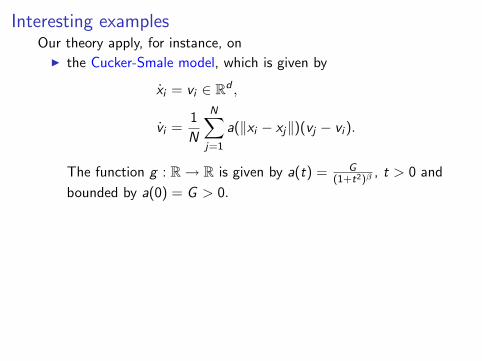
Interesting examplesOur theory apply, for instance, on
I the Cucker-Smale model, which is given by
xi = vi ∈ Rd ,
vi =1
N
N∑j=1
a(‖xi − xj‖)(vj − vi ).
The function g : R→ R is given by a(t) = G(1+t2)β
, t > 0 and
bounded by a(0) = G > 0.I the D’Orsogna-Chuang-Bertozzi-Chayes model, which is given
by
xi = vi ∈ Rd ,
vi = (a− b‖vi‖2)vi −1
N
∑j 6=i
∇U(‖xi − xj‖),
where a and b are positive constants and U : R→ R is asmooth potential.
Interesting examplesOur theory apply, for instance, on
I the Cucker-Smale model, which is given by
xi = vi ∈ Rd ,
vi =1
N
N∑j=1
a(‖xi − xj‖)(vj − vi ).
The function g : R→ R is given by a(t) = G(1+t2)β
, t > 0 and
bounded by a(0) = G > 0.
I the D’Orsogna-Chuang-Bertozzi-Chayes model, which is givenby
xi = vi ∈ Rd ,
vi = (a− b‖vi‖2)vi −1
N
∑j 6=i
∇U(‖xi − xj‖),
where a and b are positive constants and U : R→ R is asmooth potential.

Interesting examplesOur theory apply, for instance, on
I the Cucker-Smale model, which is given by
xi = vi ∈ Rd ,
vi =1
N
N∑j=1
a(‖xi − xj‖)(vj − vi ).
The function g : R→ R is given by a(t) = G(1+t2)β
, t > 0 and
bounded by a(0) = G > 0.I the D’Orsogna-Chuang-Bertozzi-Chayes model, which is given
by
xi = vi ∈ Rd ,
vi = (a− b‖vi‖2)vi −1
N
∑j 6=i
∇U(‖xi − xj‖),
where a and b are positive constants and U : R→ R is asmooth potential.

Interesting examples
In principle, we can also consider
I the Keller-Segel model, given by
dxi (t) = −c∑j 6=i
xi − xj
‖xi − xj‖ddt +
√2dBi ,
where Bi (t), i = 1, . . . ,N are mutually independentd-dimensional Brownian motions and c is a positive constant.
In this case, though, the matrix M should be better a partialorthogonal random matrix (for instance a random partial Fouriermatrix), as MBi (t), i = 1, . . . ,N are mutually independentk-dimensional Brownian motions!
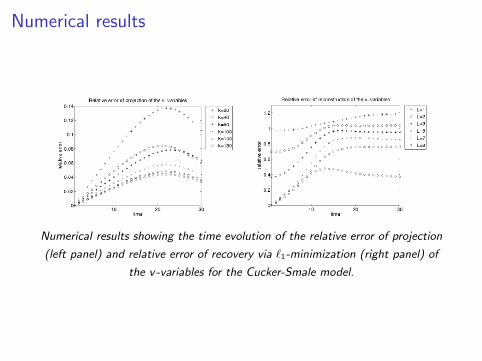
Numerical results
Numerical results showing the time evolution of the relative error of projection
(left panel) and relative error of recovery via `1-minimization (right panel) of
the v-variables for the Cucker-Smale model.

Numerical results: stability of consensus after randomprojection
Numerical results for β = 1.62: First row shows the evolution of Γ(t) = V (t)
of the CS-system projected to dimension k = 100 (left) and k = 25 (right) in
the twenty realizations, compared to the original system (bold dashed line).
Second row shows the initial values V (t = 0) and final values V (t = 30) in all
the performed simulations.

Conclusion
I We defined a general class ofdynamical systems modeling socialinteractions
I We showed that randomizedprojections via Johnson-Lindenstraussembeddings map stably thetrajectories
I We showed how `1-minimization canbe used for recoveringhigh-dimensional trajectories fromlow-dymensional simulations
I We showed an application to theCucker-Smale system modellingconsensus

A few info
I WWW: http://www-m15.ma.tum.de/
I References:I M. Caponigro, M. Fornasier, B. Piccoli, and E. Trelat, Sparse
stabilization and optimal control of the Cucker-Smale model,submitted to SIAM Review, 2012.
I J. A. Carrillo, M. Fornasier, J. Rosado, and G. Toscani,Asymptotic flocking dynamics for the kinetic Cucker-Smalemodel, SIAM. J. Math. Anal., Vol. 42, no. 1, 2010, pp.218-236.
I M. Fornasier, J. Haskovec and J. Vybıral, Particle systems andkinetic equations modeling interacting agents in highdimension, to appear in Multiscale Modeling and Simulation,2012.
I M. Fornasier and F. Solombrino, Mean field optimal control, inpreparation