Space and Time
60
1. SPACE AND TIME 1.0. Introduction It was Minkowski who paraphrased that, “... Henceforth space by itself, and time by itself, are doomed to fade away into mere shadows, and only a kind of union of the two will preserve an independent reality.” And ever since relativists are accustomed to always think in the framework of a 4-dimensional space-time, it has almost become second nature to them. Strictly speaking, however, the Minkowski signature (− + + +) makes a clear distinction as to which coordinates can be interpreted as spatial and which ones as temporal, and recently, the usefulness of 3 + 1 decomposition techniques has shown that sometimes the separation of space from time provides a better insight to what is going on rather than the traditional fusion of space with time. Imagine a universe in which nothing moves. In such a universe, the notion of time disappears. So, space and motion in space are really the primary concepts and time is a secondary concept. It should thus be possible to construct a theory of Kinematic Relativity based on the primary notions of space and motion instead of space and time. 1
Transcript of Space and Time

1. SPACE AND TIME
1.0. Introduction
It was Minkowski who paraphrased that, “. . . Henceforth space by
itself, and time by itself, are doomed to fade away into mere shadows,
and only a kind of union of the two will preserve an independent
reality.” And ever since relativists are accustomed to always think in
the framework of a 4-dimensional space-time, it has almost become
second nature to them.
Strictly speaking, however, the Minkowski signature (− + + +)
makes a clear distinction as to which coordinates can be interpreted
as spatial and which ones as temporal, and recently, the usefulness
of 3 + 1 decomposition techniques has shown that sometimes the
separation of space from time provides a better insight to what is
going on rather than the traditional fusion of space with time.
Imagine a universe in which nothing moves. In such a universe, the
notion of time disappears. So, space and motion in space are really
the primary concepts and time is a secondary concept. It should thus
be possible to construct a theory of Kinematic Relativity based on
the primary notions of space and motion instead of space and time.
1

2 Space, Time and Matter
In this monograph, we present a new formulation of both relati-
vistic kinematics and field dynamics in an entirely 3-dimensional
space. The basic idea is to represent local physical observers as
non-singular 3-dimensional local vector fields and the dynamics
of physical fields by the “flows” of the vector fields, which are
1-parameter groups of local smooth transformations of the space.
The flow parameter thus plays the role of local time for each physi-
cal observer, and Lie-derivative replaces the time derivative.
In the kinematics part, we first introduce the basic notions and
postulates of our formalism which take place in a 3-dimensional Rie-
mannian space (M3, g). A physical observer is defined to be a non-
singular vector field X on M3 with 0< g(X,X)< 1. With the help
of the metric, we can define a relative velocity function V (X,Y )
between any two physical observers X,Y . Two observers are then
inertially equivalent if V (X,Y )= const. on M3. If c : I→M3 is a
particle path, i.e., a smooth curve on M3, we can define space and
time intervals of c(I) relative to a physical observer X in such a way
that if Y is another physical observer inertially equivalent to X, then
the space and time intervals relative to Y are related to that of X by
a Lorentz transformation. The Lorentz time dilation formula is then
an immediate consequence.
We next consider the problem of constructing an equivalence class
of inertial observers starting from a representative physical observer.
The problem leads us to the definition of “generalized Lorentz
matrices” with corresponding “generalized” properties, which would
reduce to the usual Lorentz matrices when (M3, g) is an Euclidean
space.
Space and Time 3
In the dynamics part, we first show how one can describe the time
evolution of certain classical fields by subjecting the 3-dimensional
fields to a transformation by the flow of a fundamental 3-dimensional
vector field. We illustrate this with some simple 1-dimensional cases
such as the 1-dimensional Heat and Wave equations. We next apply
our basic procedure to the Gauss–Einstein equations, that is, the
Einstein field equations in Gaussian normal coordinates, and obtain
a set of equations for the 3-metric g and a 3-dimensional vector field
X. Every solution (g,X) of these equations determine uniquely a
space-time 4-metric solution of the Einstein field equations.
Our first example is the de Sitter solution. A generalization of the
de Sitter case leads us to a complex metric of Kasner type, which
in turn, provides us with a new (real) solution of the vacuum Ein-
stein field equations, containing five real parameters. We then give
another solution of our 3-dimensional equations which is mathemat-
ically interesting and non-trivial, but however, corresponds to the
physically trivial flat space-time metric. Nevertheless, this solution
clearly illustrates the basic principles of our 3-dimensional approach.
Finally, we apply our formalism to the Maxwell equations and
obtain a corresponding 3-dimensional set of equations, which turn
out to be, not only concise, but also elegant.

4 Space, Time and Matter
1.1. The Hyperbolic Structure of the Spaceof Relative Velocities
We first consider the geometry of the space of relative velocities in
conventional Special Relativity. This will suggest the formalism of a
theory of Kinematic Relativity on 3-manifolds which reproduces the
essential features of conventional relativity.
In the special theory of relativity, the velocity transformation for-
mula relating the relative velocities of three equivalent inertial sys-
tems u, v, w is given by (in units c = 1)
‖w‖2 =(u− v)2 − (u× v)2
(1− u · v)2. (1.1)
Equation (1.1) has the following geometrical significance. Let us
choose some reference inertial system and consider the velocities u =
(u1, u2, u3) of all other equivalent inertial systems relative to this
reference inertial system. Since for physical inertial systems ‖u‖ =
[|∑(ui)2|]1/2 < 1, the space of relative velocities is topologically a 3-
dimensional open disk
D3 = {u ∈ R3|‖u‖ < 1}.
Note: For tachyons, the appropriate space to consider would be the
closure of the complement of D3, that is, R3\D3.
Now, we introduce the standard (positive definite) hyperbolic met-
ric G on D3 by
ds2 =∑i,k
Gik(u)duiduk
=[1−∑(ui)2][
∑(dui)2] + [
∑uidui]2
[1−∑(ui)2]2, (1.2)
Space and Time 5
that is,
Gik(u) =[1−∑(ui)2]δik + uiuk
[1−∑(ui)2]2.
Then, H3 =(D3, G) is the standard hyperbolic 3-space of con-
stant curvature −1. This is the so-called Poincare disk model of
H3 ([1]). Alternatively, one can introduce homogeneous coordinates
ξ = (ξ0, ξ1, ξ2, ξ3) by ξi = ξ0ui and define for ξ = (ξ0, ξ1, ξ2, ξ3), η =
(η0, η1, η2, η3), the inner product (ξ, η) = ξ0η0 −∑
i ξiηi. Then,
ds2 =(dξ, ξ)(ξ, dξ) − (ξ, ξ)(dξ, dξ)
(ξ, ξ)2. (1.3)
H3 is geodesically complete and has a distance function d given by
d(u, v) = cosh−1
⎡⎢⎢⎢⎣[1−∑
iuivi
][1−∑
i(u)2
]1/2 [1−∑
i(v)2
]1/2
⎤⎥⎥⎥⎦ (1.4)
or, in homogeneous coordinates,
d(ξ, η) = cosh−1
[ |(ξ, η)|(ξ, ξ)1/2(η, η)1/2
]. (1.5)
A comparison of Eq. (1.1) with Eq. (1.5) suggests that the dis-
tance d(u, v) is somehow related to the relative velocity w between
two inertial systems whose velocities relative to the reference inertial
system are u and v. To see the actual relationship, we should note
that the reference system is at rest relative to itself. Now, from (1.4)
d(0, v) = cosh−1
[1
(1− ‖v‖2)1/2
]= tanh−1 ‖v‖.
That is, ‖v‖ = tanh d(0, v). We can, therefore, reinterpret Eq. (1.1) as
a relation between the relative velocity w and the hyperbolic distance

6 Space, Time and Matter
–4
–3
–2
–1
0
1
2
3
4
y
–4 –2 2 4x
Fig. 1. The hypersurfaces M′,M′′.
d(u, v) by
‖w‖ = tanh[d(u, v)]. (1.6)
The isometry group of H3 is intimately connected with the Lorentz
group, as can be seen in what follows.
First, we consider an abstract R4 with the Lorentz metric gR4 given
by ds2 = (dx1)2+(dx2)2+(dx3)2−(dx4)2. Consider now the hypersur-
face M of R4: M = {x = (x1, x2, x3, x4) ∈ R4|(x1)2 +(x2)2 +(x3)2−(x4)2 = −1}. M has two components: M′ = {x ∈ M|x4 ≥ 1} and
M′′ = {x ∈M|x4 ≤ −1} (see Fig. 1; here (x, y) represents (x1, x4)).
Both M′ and M′′ are diffeomorphic to D3 and the diffeomorphism
map is given by
(x1, x2, x3, x4) �→ (u1, u2, u3),
ui = xi/x4, (i = 1, 2, 3)
with its inverse
(u1, u2, u3) �→ (x1, x2, x3, x4),
xi = uix4, x4 = ±[
1(1−∑(ui)2)
]1/2
.
Space and Time 7
Now, let gM be the induced Riemannian metric on M obtained
from gR4 on R4. In coordinates (ui), gM is given exactly by (1.2).
Thus, H3 = (D3, G) is isometric to (M ′, gM |M ′) and (M ′′, gM |M ′′).
The isometry group of H3 was shown by Poincare to be PSL(2,C),
the projective special linear group in two complex dimensions and is,
thus, isomorphic to L↑+, the orthochronous Lorentz group. It is clear
from (1.5) that the isometry group of H3 leaves the inner prod-
uct (ξ, η), in homogeneous coordinates, invariant. Let its action be
given by
(ξ0, ξ1, ξ2, ξ3) �→ (ξ0, ξ1, ξ2, ξ3),
where
ξμ = Lμνξν , Lμ
ν ∈ L↑+ (μ, ν = 0, 1, 2, 3).
Since ui = ξiξ0, L↑+ acts on H3 as a fractional linear transforma-
tion:
ui �→ ui = (Li0 + Li
kuk)/(L0
0 + L0ku
k).
Thus, the fundamental aspect of the Special Theory of Relativity,
namely, Lorentz invariance, is contained in the hyperbolic structure
of the space of relative velocities.
8 Space, Time and Matter
1.2. Relativistic Kinematics on 3-Manifolds
Let (M3, g) be a 3-dimensional space with a (positive-definite) Rie-
mannian metric g. By an observer (or a particle path), we usually
mean a smooth curve in M3, i.e., a smooth map c : I → M3 from a
real interval I into M3.
Since, to every such curve c, one can associate a local vector field C
such that c is an integral curve of C ([2]). We shall regard the set of
all non-singular vector fields on M3 as the set of all observers in M3.
Non-singularity is necessary to avoid the possibility that an
observer comes to an absolute rest relative to M3. To each vector
field X corresponds a local flow χt , i.e., a local 1-parameter group
of local transformations of M3. Here, the parameter t measures the
“flow of time” as perceived by the observer represented by X. In this
sense, time is a local concept since X need not be globally defined
and is not necessarily complete unless M3 is compact ([3]).
Let us now consider only those non-singular vector fields X such
that g(X,X) < 1. Such observers will be called physical observers.
(Corresponding to the fact that no such observer can attain the veloc-
ity of light.)
From now on, we consider only physical observers and denote by
Σ(M3) the set of all physical observers.
We define a map V , called the relative velocity map, from a pair
of physical observers to a smooth function on M3 as follows:
V : Σ(M3)×Σ(M3) �→ C∞(M3),
(X,Y ) �→ V (X,Y ),

Space and Time 9
where
V (X,Y ) =[1− 1
[F (X,Y )]2
]1/2
,
F (X,Y ) =1− g(X,Y )
[1− g(X,X)]1/2 [1− g(Y, Y )]1/2.
(1.7)
Here, C∞(M3) denotes the set of all smooth functions on M3.
Let us now define an equivalence relation ∼ in Σ(M3) by:
X ∼ Y if and only if
V (X,Y ) = constant function on M3.(1.8)
In other words, the observers X and Y are said to be (inertially)
equivalent if the relative velocity function is constant on M3.
We shall now give theoretical definitions of space and time inter-
vals of a physical particle path relative to any physical observer X.
Let c : I → M3, λ �→ c(λ) be a particle path and C any represen-
tative corresponding vector field associated with it such that c is an
integral curve of C. For a physical particle path, 0 < g(C,C) < 1
on c(I).
Definition. The time interval of c relative to an observer X, denoted
by ΔtX , is given by the following integral over I:
ΔtX =∫
IF (X,C)dλ. (1.9)
Note that we can reparametrize c by tX , where dtX/dλ = F (X,C).
10 Space, Time and Matter
Definition. The space interval of c relative to the observer X,
denoted by ΔdX , is given by
ΔdX =∫
IV (X,C)dtX =
∫IV (X,C)F (X,C)dλ. (1.10)
If (ΔtY ,ΔdY ) are time and space intervals of c relative to another
observer Y , then (ΔtX ,ΔdX) → (ΔtY ,ΔdY ) provides a space-time
transformation from observer X to observer Y .

Space and Time 11
1.3. Class of Inertial Observers and GeneralizedLorentz Matrices
We now consider the problem of constructing a class of inertial
observers starting from a representative physical observer. In other
words, given a physical observer u, the problem of constructing an
observer w such that u and w are inertially equivalent, that is, the
relative velocity between u and w, V (u,w), as given by (1.7), is a
constant function on M3.
Since M3 is 3-dimensional, it is parallelizable, that is, there exists a
global “framing” of M3 by means of three linearly independent vector
fields {e(i)}, i = 1, 2, 3, so that any vector field u can be expressed
as u = ui(x)e(i), and g(e(i), e(j)) = gij(x), where ui(x), gij(x) are
functions on M3. One can, of course, also consider everything locally
in some local coordinate system (xi), so that ui(x), gij(x) are func-
tions of the coordinate (xi). Since u is a physical observer, we have
g(u, u) = gikuiuk = uiu
i < 1, where ui = gikuk.
Let
γu = [1− g(u, u)]−1/2
Au = (γu − 1)/g(u, u)
}(1.11)
and let us define the 4× 4 matrix functions Lμλ(u), μ, λ = 0, 1, 2, 3 as
followsa:
L00(u) = γu, L0
k(u) = γuuk
Lk0(u) = γuuk, Lk
j (u) = δkj + Auukuj.
⎫⎬⎭ (1.12)
Note that in (1.8) uj differ from uk by the lowering of indices by
gjk and also that Lμλ are functions on M . These “generalized Lorentz
aIn what follows Latin indices i, j, k, . . . = 1, 2, 3 and the Greek indices
α, β, γ, . . . = 0, 1, 2, 3.
12 Space, Time and Matter
matrices” Lμλ(u) are easily seen to satisfy the following “generalized”
properties:
gikLi0L
k0 = (L0
0)2 − 1
gmnLm0 Ln
i = L00L
0i
gmnLmi Ln
j = L0i L
0j + gij
⎫⎪⎪⎪⎬⎪⎪⎪⎭ (1.13)
and when (M3, g) = (R3, δ), that is, when (M3, g) is the Euclidean
space R3 with the Euclidean metric gik = δik, Lμ
λ(u) reduces to
the usual Lorentz matrix Lμλ(u) with the pure boost given by u =
(u1, u2, u3) and satisfy the usual properties:
Li0L
i0 = (L0
0)2 − 1
Lm0 Lm
i = L00L
0i
Lmi Lm
j = L0i L
0j + δij .
⎫⎪⎪⎪⎬⎪⎪⎪⎭ (1.14)
Let v = vi(x)e(i) be another vector field where g(v, v) < 1.
We now define a vector field w = wi(x)e(i) by
wi =Li
0(u) + Lik(u)vk
L00(u) + L0
k(u)vk. (1.15)
Then it follows that g(w,w) < 1, so that w also represents a physical
observer.
Using the “generalized” properties (1.9) one now shows that the
relative velocity function V (u,w) as given by (1.1) satisfies:
[V (u,w)]2 = g(v, v).
So, if v is chosen so that g(v, v) = const., the observers u and w
are inertially equivalent and, in this way, starting from u, we can
construct a class of inertially equivalent observers.

Space and Time 13
1.4. Classical Relativistic Field Dynamics
In classical field theory, the dynamics of a field is usually described
by a set of evolution equations (together possibly with some con-
straint equations) in some space-time coordinates. We shall now
demonstrate that in many cases the dynamics can also be described
in a purely spatial (i.e., 3-dimensional) setting without the neces-
sity of introducing explicitly a time-coordinate. Instead of the time-
coordinate and time-dependent quantities, the temporal evolution is
provided by the “flow” of a 3-dimensional vector field representing a
physical observer.
Before considering the Einstein field equations in some detail, we
shall first illustrate our basic approach with some simple examples
from classical field theory, such as the Heat and Wave equations. For
simplicity, we restrict our analysis to the 1-dimensional case only.
The generalization to three spatial dimensions is obvious.
1.4.1. One-dimensional Heat equation
Consider the 1-dimensional Heat equation with some initial data:
ψt = ψxx
ψ(x, 0) = φ(x).
}(1.16)
We look for solutions ψ(x, t) of (1.16) which come from the initial
data φ(x) through a transformation by the flow of a vector field
X depending on the spatial coordinate only, as follows. Let X be
given by
X = α(x)d
dx. (1.17)

14 Space, Time and Matter
Consider its integral curves given by the dynamical system
dx
dt= α(x). (1.18)
That is,∫
dt =∫
dxα(x) = ν(x), say. So that x(t) = ν−1(t + c), c =
const., and x(0) = ν−1(c) or c = ν(x(0)). The flow χt of X transforms
the initial point x(0) onto the point x(t), that is,
χt : x �→ χt(x) = ν−1(t + ν(x)). (1.19)
Now letb
ψ(x, t) = (χtφ)(x)
= φ(χt(x))
= φ(ν−1(t + ν(x)))
⎫⎪⎪⎬⎪⎪⎭ (1.20)
so that
ψ(x, 0) = φ(x).
Then ψ(x, t), which now also depends on the flow parameter t, is
the transformed initial data φ(x), which of course depends only on
the space variable x. Let us now substitute ψ(x, t) in (1.16).
Put t + ν(x) = z, and ν(x) = y. Then, ν−1′(y) = 1/ν ′(x) = α(x);
ν−1′′(y) = α′(x)α(x). And
ψt(x, t) = φ′(ν−1(z)
)ν−1′(z)
ψt(x, 0) = φ′(x)α(x) = LXφ
}(1.21)
ψx(x, t) = φ′(ν−1(z)
)ν−1′(z)ν ′(x)
ψx(x, 0) = φ′(x)ν−1′(y)ν ′(x) = φ′(x)
}(1.22)
bGeometrical objects (e.g., scalar, vector, tensor fields and densities) can be
transformed by the flow of a vector field ([3]). We could have also transformed φ(x)
by χt−1 = χ−t , by reversing the flow, that is, by letting ψ(x, t) = φ(χt
−1(x)).
This would have preserved the scalar character of φ under the flow.
Space and Time 15
ψxx(x, t) = φ′′(ν−1(z)
)[ν−1′(z)
]2[ν ′(x)
]2+ φ′(ν−1(z)
)ν−1′′(z)[ν ′(x)]2
+ φ′(ν−1(z))ν−1′(z)ν ′′(x). (1.23)
ψxx(x, 0) = φ′′(x)[ν−1′(y)
]2[ν ′(x)
]2 + φ′(x)ν−1′′(y)[ν ′(x)
]2+ φ′(x)ν−1′(y)ν ′′(x)
= φ′′(x)[α(x)
]2[α(x)
]−2
+ φ′(x)α′(x)α(x)[α(x)
]−2
−φ′(x)α(x)α′(x)[α(x)
]−2 = φ′′(x). (1.24)
If our ψ(x, t) is to satisfy (1.16), we must have
φ′(ν−1(z)
)ν−1′(z) = φ′′
(ν−1(z)
)[ν−1′(z)
]2[ν ′(x)
]2+ φ′
(ν−1(z)
)ν−1′′(z)
[ν ′(x)
]2+ φ′
(ν−1(z)
)ν−1′(z)ν ′′(x). (1.25)
Let us put ν−1(z) = u. So that again, ν−1′(z) = 1ν′(u) = α(u),
ν−1′′(z) = α′(u)α(u). We can write (1.25) as
φ′(u)α(u) =[φ′′(u)
[α(u)
]2 + φ′(u)α′(u)α(u)][
ν ′(x)]2
+ φ′(u)α(u)ν ′′(x).
The variables x and u can thus be separated to give
1− ν ′′(x)[ν ′(x)]2
=φ′′(u)φ′(u)
α(u) + α′(u)
or
[α(x)
]2 + α′(x) =φ′′(u)φ′(u)
α(u) + α′(u) = κ(const.) (1.26)
16 Space, Time and Matter
which must be satisfied for all x and u. In particular, for u = x, we
must have from (1.26)
α(x)φ′(x) = φ′′(x)
or LXφ = Δφ.
}(1.27)
Note that (1.27) also follows directly from (1.16) and the initial val-
ues in (1.21), (1.24), and that (1.27) can be obtained from (1.16)
by replacing ψ(x, t) with φ(x) and the time-derivative ∂∂t with the
Lie-derivative LX with respect to X. Any solution (φ,X) of (1.24)
provides a solution ψ of (1.16), because from (1.27), ([3]),
∂
∂tψ =
∂
∂t(χtφ) = χt(LXφ) = χt(Δφ) = Δ(χtφ) = Δψ. (1.28)
Since (1.26) or (1.27) are equations for both X and φ, the initial
data cannot be arbitrary and, therefore, our procedure provides only
special solutions of (1.16). We shall give two examples of such solu-
tions ([4]).
Example 1. φ(x) = eαx, α(x) = α = const., X = α ddx . Then (1.27)
is satisfied, and ν(x) = xα , ν−1(y) = αy, ν−1
(t + ν(x)
)= αt + x. So
ψ(x, t) = φ(ν−1(t + ν(x))
)= φ(αt + x) = eα2t+αx. From (1.26), we
get α2 = κ. If we also allow κ to be negative, we also obtain complex
solutions ψ(x, t) = eα2t±iβx with α = ±iβ.
Example 2. φ(x) = x2, α(x) = 1x , X = 1
xddx . Again, (1.27) is
satisfied and ν(x) = x2
2 , ν−1(y) = ±√2y, ν−1(t+ν(x)
)= ±√2t + x2.
So ψ(x, t) = φ(ν−1(t + ν(x))
)= φ(±√2t + x2) = 2t + x2. This is a
well-known polynomial solution of (1.16).
In fact, it is easily possible to obtain the general solution of (1.26)
or (1.27).

Space and Time 17
1.4.2. One-dimensional Wave equation
Consider now the 1-dimensional Wave equation with some initial
data:
ψtt = ψxx
ψ(x, 0) = φ(x)
ψt(x, 0) = η(x).
⎫⎪⎪⎬⎪⎪⎭ (1.29)
Again let X = α(x) ddx and its flow χt be given by (1.16), where
ν ′(x) = 1α(x) , and ψ(x, t) = φ
(ν−1(t + ν(x))
). Now since ψt(x, 0) =
LXφ, we must have
LXφ = η. (1.30)
From (1.24)
ψtt(x, t) = φ′′(ν−1(z)
)[ν−1′(z)
]2 + φ′(ν−1(z)
)ν−1′′(z)
ψtt(x, 0) = φ′′(x)[α(x)
]2 + φ′(x)α′(x)α(x).
}(1.31)
It follows from (1.24), (1.29), (1.31) that
φ′′(x)[α(x)
]2 + φ′(x)α′(x)α(x) = φ′′(x)
or LXLXφ = Δφ.
}(1.32)
Again (1.32) is obtained from (1.29) by replacing ψ(x, t) by φ(x)
and the time-derivative ∂∂t by the Lie-derivative LX . Any solution of
(1.30), (1.32) provides a solution of (1.29). Note that the initial data
φ and η now have to be related by the “constraint equation” (1.30)
and (φ,X) must satisfy (1.32). We give two special solutions of (1.30)
and (1.32), and hence of (1.29).
(i) α(x) = +1, X = ddx , ν(x) = x, ν−1
(t + ν(x)
)= t + x, ψ(x, t) =
φ(x + t) with η(x) = φ′(x),
(ii) α(x) = −1, X = − ddx , ν(x) = −x, ν−1
(t + ν(x)
)= −t + x,
ψ(x, t) = φ(x− t) with η(x) = −φ′(x).

18 Space, Time and Matter
It is also easily possible to obtain the general solution of (1.30)
and (1.29).
1.4.3. Gauss–Einstein equations
In conventional General Relativity the space-time metric gαβ satisfies
the Einstein field equations, which are basically evolution equations
with certain constraints, and it is well known ([5]) that the vacuum
Einstein field equations: Rαβ = 0 equivalent to
G0α = 0 (constraints equations)
Rik = 0 (evolution equations)
}(1.33)
provided that g00 = 0; for example, on a non-null hypersurface. Here
Gαβ ≡ Rαβ − 12gαβR is the Einstein tensor. A slight modification
is necessary if one wishes to include a non-zero cosmological con-
stant Λ in the field equations. The vacuum Einstein field equations
with a cosmological constant: Rαβ = Λgαβ also split up into a set of
constraint and a set of evolution equations and they take a particu-
larly simple form if one uses a Gaussian normal coordinate system in
which g00 = g00 = −1 and g0i = g0i = 0. Then the field equations:
R0i = 0
R00 = −Λ
Rik = Λgik
⎫⎪⎪⎬⎪⎪⎭ (1.34)
are equivalent to:
G0i = 0
G00 = −Λ
}(constraint equations)
Rik = Λgik (evolution equations)
⎫⎪⎪⎬⎪⎪⎭ (1.35)

Space and Time 19
because (1.34) implies (1.35), since G0i = g00Ri0 + g0kRik = 0 and
G00 = 1
2g00R00 − 12gikRik = 1
2Λ(g00g00 − gikgik) = −Λ.
Conversely, (1.35) implies (1.34), since if G0i = g00Ri0+g0kRik = 0,
then from (1.35) Ri0 = 0; and if G00 = 1
2g00R00− 12gikRik = −Λ, then
from (1.35), 12g00R00 − 3
2Λ = −Λ, that is, R00 = −Λ.
The corresponding matter field equations with an energy momen-
tum tensor Tαβ : Gαβ + Λgαβ + Tαβ = 0 or, equivalently, Rαβ =12Tgαβ − Tαβ + Λgαβ take the following form (in the case of dustlike
matter with density ρ, pressure p = 0, and also in a Gaussian normal
coordinate system):
R0i = 0
R00 = −12ρ− Λ
Rik =(−1
2ρ + Λ
)gik.
⎫⎪⎪⎪⎪⎪⎪⎬⎪⎪⎪⎪⎪⎪⎭(1.36)
Equation (1.36) is then equivalent to
⎧⎪⎪⎪⎪⎨⎪⎪⎪⎪⎩G0
i = 0
G00 = ρ− Λ
}(constraint equations)
Rik =(−1
2ρ + Λ
)gik (evolution equations).
⎫⎪⎪⎪⎪⎬⎪⎪⎪⎪⎭(1.37)
Gaussian normal coordinates can be introduced in general always,
and with x = (x0 = t, x1, x2, x3), the metric takes the form: ds2 =
−dt2 + gik(x)dxidxk. So that g00 = g00 = −1, g0i = g0i = 0. The
4-metric gαβ thus determines a 3-metric gik, with its inverse gik,
which is positive definite on the hypersurfaces t = const. The field
equations (1.34) are then explicitly, in a Gaussian normal coordinate
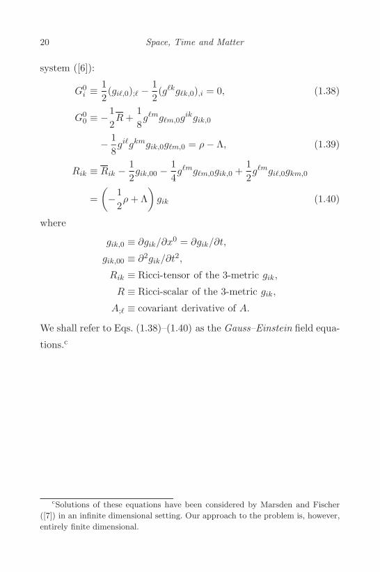
20 Space, Time and Matter
system ([6]):
G0i ≡
12(gi�,0);� − 1
2(g�kg�k,0),i = 0, (1.38)
G00 ≡ −
12R +
18g�mg�m,0g
ikgik,0
− 18gi�gkmgik,0g�m,0 = ρ− Λ, (1.39)
Rik ≡ Rik − 12gik,00 − 1
4g�mg�m,0gik,0 +
12g�mgi�,0gkm,0
=(−1
2ρ + Λ
)gik (1.40)
where
gik,0 ≡ ∂gik/∂x0 = ∂gik/∂t,
gik,00 ≡ ∂2gik/∂t2,
Rik ≡ Ricci-tensor of the 3-metric gik,
R ≡ Ricci-scalar of the 3-metric gik,
A;� ≡ covariant derivative of A.
We shall refer to Eqs. (1.38)–(1.40) as the Gauss–Einstein field equa-
tions.c
cSolutions of these equations have been considered by Marsden and Fischer
([7]) in an infinite dimensional setting. Our approach to the problem is, however,
entirely finite dimensional.
Space and Time 21
1.5. Relativistic Field Dynamics on 3-Manifolds
1.5.1. Three-dimensional field equations andrelationship with Einstein equations
As we have seen that in classical field theory, the dynamics of a field
is usually described by a set of evolution equations (together pos-
sibly with some constraint equations) in some space-time manifold.
We shall now demonstrate that in many cases the dynamics can also
be described in a purely 3-dimensional setting without the neces-
sity of explicitly introducing a time-coordinate. Instead of the time-
coordinate and time-dependent quantities, the temporal evolution is
provided by the “flow” of a 3-dimensional vector field representing a
fundamental observer.
The starting point of our dynamical theory would be a set of dif-
ferential equations for a 3-metric g and a fundamental 3-vector field
X on a M3. Let X = Xi(x)∂/∂xi be a vector field on M3 (in some
local coordinate system (xi)), and h = LXg, the Lie-derivative of g
with respect to X.
So that
h = hikdxi ⊗ dxk where hik = (LXg)ik.
Let
f,i, f;i ≡ partial and covariant derivative of f , respectively,
Rik ≡ Ricci-tensor of the 3-metric gik,
R ≡ Ricci-scalar of the 3-metric gik.
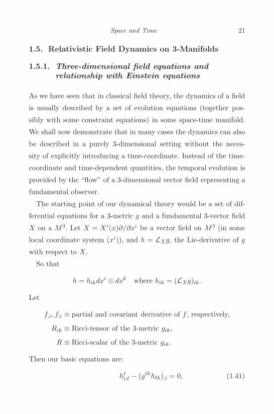
Then our basic equations are:
h�i;� − (g�kh�k),i = 0, (1.41)

22 Space, Time and Matter
−12R +
18(g�mh�m)(gikhik)
− 18(gi�hik)(gkmh�m) = 0, (1.42)
Rik − 12(LXh)ik − 1
4(g�mh�m)hik
+12(g�mhi�)hkm = 0. (1.43)
We regard Eqs. (1.41)–(1.43) as a set of differential equations for
both the 3-metric g and the 3-dimensional vector field X on M3.
Every solution (g,X) of (1.41)–(1.43) determines uniquely a solution
of the vacuum Einstein field equations as follows:
The integral curves of X determine a flow ϕτ , which are local
1-parameter group of local diffeomorphisms ([5]) of M3. Thus, for
each value of the flow parameter τ , ϕτ defines a point transformation:
x �→ x = ϕτ (x) with ϕ0(x) = x. The flow transformed metric g =
ϕτ (g) is given by gik(τ, x) = ∂x�
∂xi∂xm
∂xk g�m(x), and is thus τ -dependent.
Theorem 1. Let (gik;Xi) be a solution of (1.9)−(1.11) and
gik(τ, x) the τ -dependent metric transformed by the flow ϕτ of X.
Then, the 4-dimensional metric,
ds2 = −dτ2 + gik(τ, x)dxidxk (1.44)
is a solution of the vacuum Einstein equations in a Gaussian normal
coordinate system (x0 = τ, xi).
Proof. Let
K ≡ any tensor field,
ϕτ (K) ≡ the flow transformed tensor field K,
LXK ≡ the Lie-derivative of K with respect to X.
Space and Time 23
Then one has ([5])
ϕτ (LXK) =∂
∂τ(ϕτ (K)). (1.45)
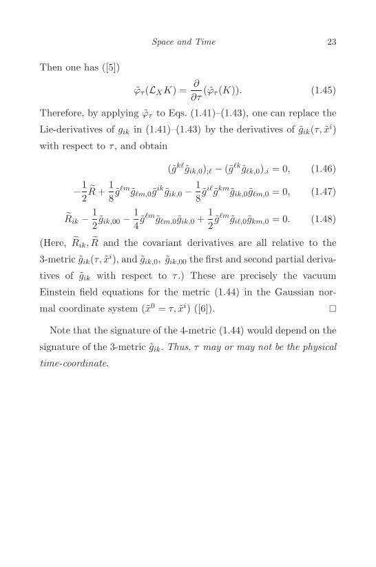
Therefore, by applying ϕτ to Eqs. (1.41)–(1.43), one can replace the
Lie-derivatives of gik in (1.41)–(1.43) by the derivatives of gik(τ, xi)
with respect to τ , and obtain
(gk�gik,0);� − (g�kg�k,0),i = 0, (1.46)
−12R +
18g�mg�m,0g
ikgik,0 − 18gi�gkmgik,0g�m,0 = 0, (1.47)
Rik − 12gik,00 − 1
4g�mg�m,0gik,0 +
12g�mgi�,0gkm,0 = 0. (1.48)
(Here, Rik, R and the covariant derivatives are all relative to the
3-metric gik(τ, xi), and gik,0, gik,00 the first and second partial deriva-
tives of gik with respect to τ .) These are precisely the vacuum
Einstein field equations for the metric (1.44) in the Gaussian nor-
mal coordinate system (x0 = τ, xi) ([6]). �
Note that the signature of the 4-metric (1.44) would depend on the
signature of the 3-metric gik. Thus, τ may or may not be the physical
time-coordinate.
24 Space, Time and Matter
1.6. Flat-Space Solutions
We now consider some special solutions of (1.41)–(1.43). First, note
that if, either X = 0 or X is a Killing vector field of g, then h =
LXg = 0. So that (1.41) is identically satisfied. Furthermore, if ρ =
Λ = 0, then (1.43) implies that Rik = 0 which in turn implies that
Rijk� = 0 (since M3 is 3-dimensional), that is, M3 is flat with the
metric g = δ (i.e., gik = δik in some coordinate system). So, {X = 0,
g = δ} and {X is Killing, g = δ} are both solutions of (1.41)–(1.43)
with ρ = Λ = 0. These are trivial flat-space solutions.
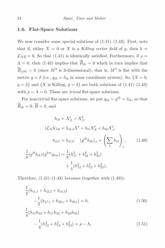
For non-trivial flat-space solutions, we put gik = gik = δik, so that
Rik = 0, R = 0, and
hik = Xi,k + Xk
,i,
(LXh)ik = hik,�X� + h�iX
�,k + h�kX
�,i,
hi�;� = hi�,�; (g�kh�k),i =
(∑�
h��
),i
, (1.49)
18(gi�hik)(gkmg�m) =
18(h2
11 + h222 + h2
33)
+14(h2
12 + h213 + h2
23).
Therefore, (1.41)–(1.43) becomes (together with (1.49)):
12(hi1,1 + hi2,2 + hi3,3)
−12(h11,i + h22,i + h33,i) = 0, (1.50)
14(h11h22 + h11h33 + h22h33)
− 14(h2
12 + h213 + h2
23) = ρ− Λ, (1.51)

Space and Time 25
− 12(hik,�X
� + h�iX�,k + h�kX
�,i) +
12(hi1hk1 + hi2hk2 + hi3hk3)
− 14(h11 + h22 + h33)hik =
(−1
2ρ + Λ
)δik. (1.52)
In terms of Xi and its derivatives, Eqs. (1.50)–(1.52) are
12(Xi
,� + X�,i),� − (X�
,�),i = 0, (1.53)
12(Xi
,i)2 − 1
8(Xi
,m + Xm,i )(Xm
,i + Xi,m) = ρ− Λ, (1.54)
− 12(Xi
,k + Xk,i),�X
� − 12(Xi
,� + X�,i)X
�,k
− 12(X�
,k + Xk,�)X
�,i
− 12X�
,�(Xi,k + Xk
,i) +12(Xi
,m + Xm,i )(Xm
,k + Xk,m)
=(−1
2ρ + Λ
)δik. (1.55)
In spite of the complexity of the above equations, it is possible to
find some non-trivial solutions as we shall see next.

26 Space, Time and Matter
1.7. The de Sitter Solution
As a non-trivial solution of (1.53)–(1.55) or (1.49)–(1.52), let ρ = 0
and Xi = −λxi, where λ is a constant to be determined. Then by
(1.49) (LXg)ik = hik = −2λδik and
−12(LXh)ik = −1
2[−λh�ix
�,k − λh�kx
�,i] = −2λ2δik,
−14(g�mh�m)hik = −1
4(δ�mh�m)hik = −3λ2δik,
12(g�mhi�)hkm =
12(δ�mhi�)hkm = 2λ2δik.
So (1.50) is identically satisfied and (1.51)–(1.52) or (1.42)–(1.43),
become
3λ2 = −Λ, (1.56)
−2λ2δik + 2λ2δik − 3λ2δik = Λδik. (1.57)
These equations are satisfied by taking λ =√−Λ3 . So that {g = δ,
X = −√−Λ3 xi ∂
∂xi }, ρ = 0 is a solution of (1.49)–(1.52), that is, a
flat-space solution of (1.41)–(1.43).
The flow generated by the vector field X = −λxi ∂∂xi is simply
xi �→ xi = e−λtxi, so that ∂xi
∂xk = eλtδik and the transformed time-
dependent 3-metric is therefore gik(x, t) = e2λtδik. The corresponding
4-metric (in coordinates (t, xi)):
ds2 = −dt2 + gikdxidxk = −dt2 + e2λtδikdxidxk
with λ =√−Λ3 is the well-known de Sitter solution of the Gauss–
Einstein equations (with ρ = 0).

Space and Time 27
1.8. A New Solution of the Vacuum EinsteinField Equations
As our next non-trivial solution of (1.49)–(1.52), we make the ansatz:
ρ = Λ = 0 and X1 = −λ1x1, X2 = −λ2x
2, X3 = −λ3x3, i.e., Xi =
−λixi (no summation), where λi’s are constants to be determined.
Then hik = −(λi + λk)δik (no summation), i.e., h11 = −2λ1, h22 =
−2λ2, h33 = −2λ3, hik = 0 if i = k.
Again, (1.50) is identically satisfied, and (1.51) implies
λ1λ2 + λ1λ3 + λ2λ3 = 0. (1.58)
Now −12(LXh)ik = −1
2(h�iX�,k + h�kX
�,i). If i = k, for example,
i = 1, k = 2, −12(LXh)12 = 0, 1
2 (h11h21 + h12h22 + h13h23) = 0 and
−14(h11 + h22 + h33)h12 = 0. So that (1.52) is identically satisfied
if i = k. If i = k, for example, i = 1, k = 1, −12(LXh)11 = −2λ2
1,12(h11h11 + h12h12 + h13h13) = 2λ2
1 and −14(h11 + h22 + h33)h11 =
−λ1(λ1 + λ2 + λ3). So that (1.52) implies
−λ1(λ1 + λ2 + λ3) = 0
−λ2(λ1 + λ2 + λ3) = 0
−λ3(λ1 + λ2 + λ3) = 0.
⎫⎪⎪⎬⎪⎪⎭So, we would have a solution of the form Xi = −λix
i (no summation)
provided
λ1 + λ2 + λ3 = 0
and
λ1λ2 + λ1λ3 + λ2λ3 = 0
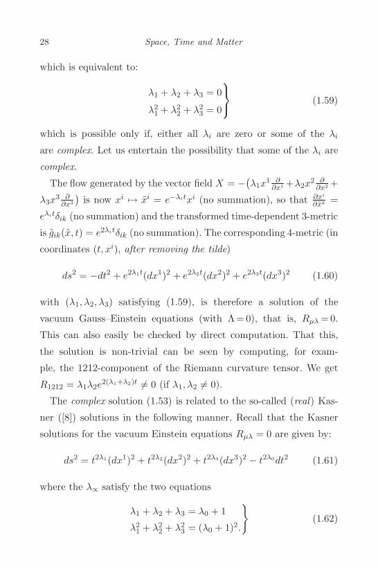
28 Space, Time and Matter
which is equivalent to:
λ1 + λ2 + λ3 = 0
λ21 + λ2
2 + λ23 = 0
⎫⎬⎭ (1.59)
which is possible only if, either all λi are zero or some of the λi
are complex. Let us entertain the possibility that some of the λi are
complex.
The flow generated by the vector field X = −(λ1x1 ∂
∂x1 +λ2x2 ∂
∂x2 +
λ3x3 ∂
∂x3
)is now xi �→ xi = e−λitxi (no summation), so that ∂xi
∂xk =
eλitδik (no summation) and the transformed time-dependent 3-metric
is gik(x, t) = e2λitδik (no summation). The corresponding 4-metric (in
coordinates (t, xi), after removing the tilde)
ds2 = −dt2 + e2λ1t(dx1)2 + e2λ2t(dx2)2 + e2λ3t(dx3)2 (1.60)
with (λ1, λ2, λ3) satisfying (1.59), is therefore a solution of the
vacuum Gauss–Einstein equations (with Λ= 0), that is, Rμλ = 0.
This can also easily be checked by direct computation. That this,
the solution is non-trivial can be seen by computing, for exam-
ple, the 1212-component of the Riemann curvature tensor. We get
R1212 = λ1λ2e2(λ1+λ2)t = 0 (if λ1, λ2 = 0).
The complex solution (1.53) is related to the so-called (real) Kas-
ner ([8]) solutions in the following manner. Recall that the Kasner
solutions for the vacuum Einstein equations Rμλ = 0 are given by:
ds2 = t2λ1(dx1)2 + t2λ2(dx2)2 + t2λ3(dx3)2 − t2λ0dt2 (1.61)
where the λ∝ satisfy the two equations
λ1 + λ2 + λ3 = λ0 + 1
λ21 + λ2
2 + λ23 = (λ0 + 1)2.
}(1.62)

Space and Time 29
If one takes λ0 = 0, one gets the standard Kasner solution
ds2 = −dt2 + t2λ1(dx1)2 + t2λ2(dx2)2 + t2λ3(dx3)2 (1.63)
with
λ1 + λ2 + λ3 = 1
λ21 + λ2
2 + λ23 = 1.
}(1.64)
A special solution of (1.64) is λ1 = 23 , λ2 = 2
3 , λ3 = −13 . The other
obvious special solution λ1 = 1, λ2 = λ3 = 0, i.e.,
ds2 = −dt2 + t2(dx1)2 + (dx2)2 + (dx3)2 (1.65)
is actually a flat metric as can be seen by the following transformation
of coordinates: t = t cosh x1, x = t sinhx1, x2 = x2, x3 = x3, which
transforms (1.65) into
ds2 = −dt 2 + (dx1)2 + (dx2)2 + (dx3)2.
If we replace t by t = et in (1.61), we get
ds2 = e2λ1 t(dx1)2 + e2λ2 t(dx2)2 + e2λ3 t(dx3)2 − e2(λ0+1)t(dt )2. (1.66)
If we now take λ0 = −1 in (1.62) and (1.66), we get precisely
(1.60), with t instead of t,
ds2 = e2λ1 t(dx1)2 + e2λ2 t(dx2)2 + e2λ3 t(dx3)2 − (dt )2
with
λ1 + λ2 + λ3 = 0
λ21 + λ2
2 + λ23 = 0.
}(1.59)
Consider now the complex solutions of (1.59). They are
λ1 =12(−1 + i
√3)λ3
λ2 =12(−1− i
√3)λ3
⎫⎪⎪⎬⎪⎪⎭ (1.67)
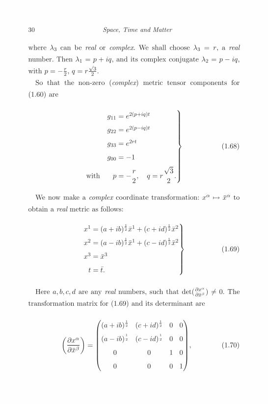
30 Space, Time and Matter
where λ3 can be real or complex. We shall choose λ3 = r, a real
number. Then λ1 = p + iq, and its complex conjugate λ2 = p − iq,
with p = − r2 , q = r
√3
2 .
So that the non-zero (complex) metric tensor components for
(1.60) are
g11 = e2(p+iq)t
g22 = e2(p−iq)t
g33 = e2rt
g00 = −1
with p = −r
2, q = r
√3
2.
⎫⎪⎪⎪⎪⎪⎪⎪⎪⎪⎪⎪⎬⎪⎪⎪⎪⎪⎪⎪⎪⎪⎪⎪⎭(1.68)
We now make a complex coordinate transformation: xα �→ xα to
obtain a real metric as follows:
x1 = (a + ib)12 x1 + (c + id)
12 x2
x2 = (a− ib)12 x1 + (c− id)
12 x2
x3 = x3
t = t.
⎫⎪⎪⎪⎪⎪⎪⎬⎪⎪⎪⎪⎪⎪⎭(1.69)
Here a, b, c, d are any real numbers, such that det(∂xα
∂xβ ) = 0. The
transformation matrix for (1.69) and its determinant are
(∂xα
∂xβ
)=
⎛⎜⎜⎜⎜⎜⎜⎝(a + ib)
12 (c + id)
12 0 0
(a− ib)12 (c− id)
12 0 0
0 0 1 0
0 0 0 1
⎞⎟⎟⎟⎟⎟⎟⎠, (1.70)
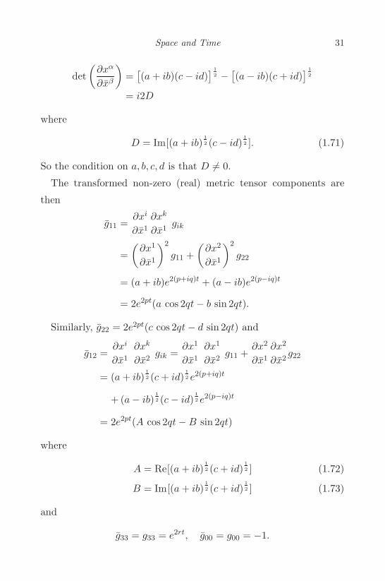
Space and Time 31
det(
∂xα
∂xβ
)=[(a + ib)(c − id)
] 12 − [(a− ib)(c + id)
] 12
= i2D
where
D = Im[(a + ib)12 (c− id)
12 ]. (1.71)
So the condition on a, b, c, d is that D = 0.
The transformed non-zero (real) metric tensor components are
then
g11 =∂xi
∂x1
∂xk
∂x1gik
=(
∂x1
∂x1
)2
g11 +(
∂x2
∂x1
)2
g22
= (a + ib)e2(p+iq)t + (a− ib)e2(p−iq)t
= 2e2pt(a cos 2qt− b sin 2qt).
Similarly, g22 = 2e2pt(c cos 2qt− d sin 2qt) and
g12 =∂xi
∂x1
∂xk
∂x2gik =
∂x1
∂x1
∂x1
∂x2g11 +
∂x2
∂x1
∂x2
∂x2g22
= (a + ib)12 (c + id)
12 e2(p+iq)t
+ (a− ib)12 (c− id)
12 e2(p−iq)t
= 2e2pt(A cos 2qt−B sin 2qt)
where
A = Re[(a + ib)12 (c + id)
12 ] (1.72)
B = Im[(a + ib)12 (c + id)
12 ] (1.73)
and
g33 = g33 = e2rt, g00 = g00 = −1.
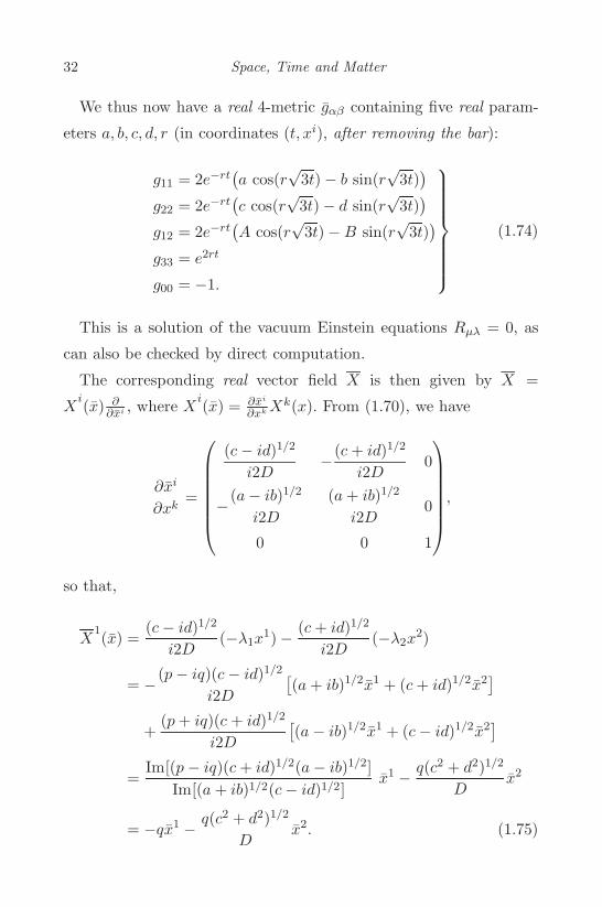
32 Space, Time and Matter
We thus now have a real 4-metric gαβ containing five real param-
eters a, b, c, d, r (in coordinates (t, xi), after removing the bar):
g11 = 2e−rt(a cos(r
√3t)− b sin(r
√3t))
g22 = 2e−rt(c cos(r
√3t)− d sin(r
√3t))
g12 = 2e−rt(A cos(r
√3t)−B sin(r
√3t))
g33 = e2rt
g00 = −1.
⎫⎪⎪⎪⎪⎪⎪⎪⎬⎪⎪⎪⎪⎪⎪⎪⎭(1.74)
This is a solution of the vacuum Einstein equations Rμλ = 0, as
can also be checked by direct computation.
The corresponding real vector field X is then given by X =
Xi(x) ∂
∂xi , where Xi(x) = ∂xi
∂xk Xk(x). From (1.70), we have
∂xi
∂xk=
⎛⎜⎜⎜⎜⎜⎜⎝(c− id)1/2
i2D−(c + id)1/2
i2D0
−(a− ib)1/2
i2D(a + ib)1/2
i2D0
0 0 1
⎞⎟⎟⎟⎟⎟⎟⎠,
so that,
X1(x) =
(c− id)1/2
i2D(−λ1x
1)− (c + id)1/2
i2D(−λ2x
2)
= −(p− iq)(c− id)1/2
i2D[(a + ib)1/2x1 + (c + id)1/2x2
]+
(p + iq)(c + id)1/2
i2D[(a− ib)1/2x1 + (c− id)1/2x2
]=
Im[(p − iq)(c + id)1/2(a− ib)1/2]Im[(a + ib)1/2(c− id)1/2]
x1 − q(c2 + d2)1/2
Dx2
= −qx1 − q(c2 + d2)1/2
Dx2. (1.75)

Space and Time 33
Similarly, X2(x) = q(a2+b2)1/2
D x1 + qx2 and X3(x) = −rx3. After
removing the bar again, the real vector field X is given by
X =
(−qx1 − q(c2 + d2)1/2
Dx2
)∂
∂x1
+
(q(a2 + b2)1/2
Dx1 + qx2
)∂
∂x2− rx3 ∂
∂x3. (1.76)
We, thus, have a real solution (g,X) of (1.41)–(1.43) with g = δ
and X given by (1.76).
A special case of (1.74) is given by a = 1, b = c = 0, d = 1 with
A = B = 1/√
2,D = −1/√
2,
g11 = 2e−rτ cos(r√
3τ)
g22 = −2e−rτ sin(r√
3τ)
g12 =√
2e−rτ(cos(r
√3τ)− sin(r
√3τ))
g33 = e2rτ
g00 = −1.
⎫⎪⎪⎪⎪⎪⎪⎪⎬⎪⎪⎪⎪⎪⎪⎪⎭(1.77)
This solution can also be checked by direct calculation.d
Notes on signature: The signature of the metric (1.77) is non-
Lorentzian and the vector field X is real. A Lorentzian metric is
obtained by changing the sign of g33, i.e., g33 = −e2rτ . This can be
achieved by taking x3 = ix3 in (1.69). However, then, the correspond-
ing vector field has to be complex. In both cases, the corresponding
3-metrics must have indefinite signatures.
dThis was done on MAPLE, the symbolic computation language. See
Appendix C.
34 Space, Time and Matter
1.9. A Solution of Mathematical Interest
We present now another solution of our equations which is mathe-
matically interesting but turns out to be physically trivial. However,
this solution illustrates the basic principle of our approach.
Again, suppose ρ = Λ = 0 and now we assume
hik = λiλkf (1.78)
where λi are constants and f is a function of (xi) to be determined.
Then (1.51) is identically satisfied, whereas (1.50) implies
12(λiλ1f,1 + λiλ2f,2 + λiλ3f,3)− 1
2(λ2
1 + λ22 + λ2
3)f,i = 0. (1.79)
We can satisfy (1.71) by assuming
λif,k = λkf,i (1.80)
which implies that
f(x) = F (u), where u = λixi (1.81)
and F is a function of the single variable u. Now, consider Eq. (1.52)
in view of (1.78) and (1.80). It becomes
12(LXh)ik =
14λiλkf
2∑
j
λ2j
or
λiλkf,�X� + λiλ�fX�
,k + λkλ�fX�,i =
12λiλkf
2∑
j
λ2j . (1.82)
Let us put
Xi =12λiG(u). (1.83)

Space and Time 35
Then
hik = Xi,k + Xk
,i = λiλkG′,
so that
F = G′ (1.84)
and (1.82) becomes
(F ′G + 2FG′)∑
j
λj = F 2∑
j
λ2j ,
or[G′′G + 2(G′)2
]∑j
λj = (G′)2∑
j
λ2j .
(1.85)
We can satisfy (1.85) by taking, say,∑j
λj =∑
j
λ2j = 1 (1.86)
and by making sure that G satisfies the following equation
G′′G + (G′)2 = 0, (1.87)
the general solution of which is: G(u) = ±(au + b)12 , where a, b are
arbitrary constants.
A solution of (1.49)–(1.52) is thus provided by (g,X) where g = δ
and X = Xi(x)δ/δxi with Xi(x) = 12λiu
1/2, where λi satisfy (1.86)
and u = λixi. Next, we shall derive the corresponding 4-metric solu-
tion of the vacuum field equations (1.38)–(1.40) by transforming the
3-metric g = δ by the flow of X. The flow of X is given by the
solution of the dynamical system:
dxi
dt=
12λiu
12 = λi(λ1x
1 + λ2x2 + λ3x
3)12
xi(0) = xi0
⎫⎪⎬⎪⎭ (1.88)

36 Space, Time and Matter
together with (1.86). To solve (1.88), note that, according to (1.86)
and (1.88) dudt = λi
dxi
dt = 12(Σiλ
2i )u
12 = 1
2u12 and u(0) = u0 = λix
i0.
This implies that u12 = t
4 + u120 , and so
x2(t) =∫
12λ2
(t
4+ u
120
)dt = x2
0 +12λ2u
120 t +
116
λ2t2,
x3(t) =∫
12λ3
(t
4+ u
120
)dt = x3
0 +12λ3u
120 t +
116
λ3t2,
x1(t) =u
λ1− λ2
λ1x2(t)− λ3
λ1x3(t)
=1λ1
(t
4+ u
120
)2
− λ2
λ1
(x2
0 +12λ2u
120 t +
116
λ2t2
)− λ3
λ1
(x3
0 +12λ3u
120 t +
116
λ3t2
)= x1
0 +12λ1u
120 +
116
λ1t2.
Under the flow of X, the point (xi0) is mapped into the
point (xi(t)). The flow generated by X is thus χt : xi �→ xi = xi+12λiu
12 t + 1
16λit2. The inverse transformation is: xi �→ xi = xi −
12λi(u1/2− t
4)t− 116λit
2, where u = λixi. In view of (1.86), the Jacobian
matrix of the transformation turns out to be
∂xi
∂xk= δik − λiλkω; ω = t/4(λix
i)12
with det(
∂xi
∂xk
)= 1− w.
⎫⎪⎪⎪⎬⎪⎪⎪⎭ (1.89)
Under the flow of X, the flat 3-metric gik(x) = δik is transformed
into gik(x, t), according to:
gik(x, t) =∂x�
∂xi
∂xm
∂xkδ�m.

Space and Time 37
Thus,
gik(x, t) = δik + λiλkω2 − 2λiλkω. (1.90)
And, we have a 4-metric solution gαβ of the vacuum field equations
Rαβ = 0 (in coordinates (t, xi), after removing the tilde in (1.90))
gαβ =
(δik + λiλkω
2 − 2λiλkω 0
0 −1
)
ω = t/4(λixi)
12 ;
∑i
λi =∑
i
λ2i = 1
(1.91)
with det(gαβ) = −(1 − ω)2. However, not only Rαβ = 0, but also
Rαβγδ = 0. The solution thus represents a flat space-time!
38 Space, Time and Matter
1.10. The Schwarzschild Solution
As the first example of a non-trivial flat 3-space solution of (1.41)–
(1.43), consider a general spherically symmetric 3-metric g and a
spherically symmetric vector field X in coordinates (x1 = ρ, x2 =
θ, x3 = φ):
g = gikdxidxk = f(ρ)2dρ2 + ρ2(dθ2 + sin2 θdφ2),
X = Xi ∂
∂xi= a(ρ)
∂
∂ρ.
(1.92)
Substituting (1.92) in (1.41)–(1.43), we obtain the following
ordinary differential equations for the unknown functions f(ρ)
and a(ρ)
4
(d
dρf(ρ)
)a(ρ)
f(ρ)ρ= 0, (1.93)
42(
d
dρf(ρ)
)ρ + (f(ρ))3 − f(ρ) + 2 ρ
(d
dρf(ρ)
)(a(ρ))2(f(ρ))2
ρ2(f(ρ))3
+ 42 ρ(f(ρ))3
(d
dρa(ρ)
)a(ρ) + (a(ρ))2(f(ρ))3
ρ2(f(ρ))3= 0, (1.94)
−(
2d
dρf(ρ) + (f(ρ))2
(d2
dρ2f(ρ)
)(a(ρ))2 ρ
+ 3(
d
dρf(ρ)
)a(ρ) (f(ρ))2
(d
dρa(ρ)
)ρ
)× (f(ρ)ρ)−1
−a(ρ)(f(ρ))3
(d2
dρ2a(ρ)
)ρ + (f(ρ))3
(d
dρa(ρ)
)2
ρ
f(ρ)ρ

Space and Time 39
−2(
d
dρf(ρ)
)(a(ρ))2(f(ρ))2 + 2(f(ρ))3
(d
dρa(ρ)
)a(ρ)
f(ρ)ρ= 0,
(1.95)
−
(d
dρf(ρ)
)ρ + (f(ρ))3 − f(ρ) + (a(ρ))2(f(ρ))3
(f(ρ))3
−2 ρ(f(ρ))3
(d
dρa(ρ)
)a(ρ) + ρ
(d
dρf(ρ)
)(a(ρ))2(f(ρ))2
(f(ρ))3= 0.
(1.96)
[Eq. (1.96)] (sin(θ))2. (1.97)
Equation (1.93) implies that, for non-trivial a(ρ), f(ρ) = const.
(which we set equal to one). Equation (1.94) then becomes
2(
d
dρa(ρ)
)a(ρ)ρ
+a(ρ)2
ρ2= 0 (1.98)
whose solution is a(ρ) = kρ1/2 , k = const. The remaining Eqs. (1.95)–
(1.97) are then identically satisfied.
Thus the flat 3-metric
g = dρ2 + ρ2(dθ2 + sin2 θdφ2)
and the vector field X = kρ−12
∂
∂ρ
⎫⎪⎬⎪⎭ (1.99)
is the only solution of Eqs. (1.93)–(1.97).
1.10.1. The Schwarzschild metric
We now wish to derive the space-time 4-metric which corresponds
to our solution (1.99), according to Theorem 1, by transforming the
3-metric g by the flow of the vector field X. In order to calculate

40 Space, Time and Matter
the flow of X, it is convenient to transform X first to a simpler form
by a simple change of coordinates. For example, the transformation
(ρ, θ, φ) �→ (R, θ, φ), where ρ = (32kR)
23 transforms the metric as
well as the vector field in (1.99), into
g = k2
(32kR
)− 23
dR2 +(
32kR
) 43
(dθ2 + sin2 θdφ2)
X =∂
∂R.
⎫⎪⎪⎬⎪⎪⎭ (1.100)
It is clear from the invariant form of Eqs. (1.41)–(1.43), that a
change of coordinates provides another solution of the metric and
the vector field. It can also be checked directly that (1.100) is indeed
a solution of (1.41)–(1.43). And, of course, the 3-metric in (1.100) is
still flat.
The flow ϕτ of X is given by: ϕτ : R �→ R = R + τ , θ �→ θ = θ,
φ �→ φ = φ. Therefore, according to Theorem 1, (1.25) corresponds to
the space-time 4-metric (in Gaussian normal coordinates (τ, R, θ, φ)):
ds2 = −dτ2 + k2
[32k(R− τ)
]− 23
dR2
+[32k(R − τ)
] 43
(dθ2 + sin2 θdφ2). (1.101)
That (1.101) is a solution of the vacuum Einstein field equations
can also be checked directly. In fact, (1.101) is the Schwarzschild
solution in the so-called Lemaitre coordinates ([9–11]) if we take
k = (2m)12 .
This can be seen by considering the following transformation:
(τ, R, θ, φ) �→ (t, r, θ, φ),

Space and Time 41
where
τ = 2( r
2m
) 12 + 2m log
∣∣∣∣∣√
r −√2m√r +
√2m
∣∣∣∣∣− t = τ(r, t)
R =23r
32 (2m)−
12 + τ = R(r, t)
θ = θ, φ = φ
⎫⎪⎪⎪⎪⎪⎪⎪⎬⎪⎪⎪⎪⎪⎪⎪⎭(1.102)
with the inverse transformation:
(t, r, θ, φ) �→ (τ, R, θ, φ),
where
r = (2m)13
[32(R− τ)
] 23
= r(R, τ)
t = 2( r
2m
) 12 + 2m log
∣∣∣∣∣√
r −√2m√r +
√2m
∣∣∣∣∣− τ = t(R, τ)
θ = θ, φ = φ.
⎫⎪⎪⎪⎪⎪⎪⎪⎪⎬⎪⎪⎪⎪⎪⎪⎪⎪⎭(1.103)
(1.102) or (1.103) transforms (1.101) into the Schwarzschild metric:
ds2 = −(
1− 2mr
)dt2 +
(1− 2m
r
)−1
dr2 + r2(dθ2 + sin2 θdφ2).
(1.104)
Incidentally, we have thus proved a version of Birkoff’s Theorem in
our formalism, namely, that the only spherically symmetric solution
of (1.41)–(1.43) leads to the Schwarzschild space-time.
One might think that if (X, g) is a solution of (1.41)–(1.43), then
adding a Killing vector field of g to X would again give us another
solution. In fact, one has the following proposition.
Proposition 1. Let (X, g) be a solution and X0 a Killing vector
field of g. Then, (X + X0, g) is also a solution provided [X,X0] = 0.
42 Space, Time and Matter
Proof. Let X = X + X0. Then, LXg = LXg and LX(LXg) =
LX(LXg)+LX0(LXg). Now, [LX0 ,LX ] = L[X0,X]. Hence, [X0,X] = 0
implies that LX0(LXg) = LX(LX0g) = 0, and therefore, we have also
LX(LXg) = LX(LXg). �
However, this does not generate a new space-time 4-metric in view
of the following Proposition.
Proposition 2. (X, g) and (X + X0, g), where [X,X0] = 0, gener-
ate equivalent space-time 4-metrics.
Proof. Since X commutes with X0, the flow of X + X0 is a com-
position (as maps) of the flow of X and the flow of X0. Since X0 is
Killing, the flow of X0 has no effect on the metric g. Therefore, the
effect of the flow of X + X0 on g is the same as that of X. �
For example, consider the solution (1.99) together with the two
Killing vectors X0 and X1 of the 3-metric:
g: ds2 = dρ2 + ρ2(dθ2 + sin2 θdφ2),
X = (2m/ρ)12
∂
∂ρ,
X0 = sinφ∂
∂θ+ cot θ cos φ
∂
∂φ,
X1 = sin θ cos φ∂
∂ρ+ (cos θ cos φ/ρ)
∂
∂θ
− (cosec θ sin φ/ρ)∂
∂φ.
Here, the Killing vector field X0 corresponds to rotational isometry,
whereas X1 corresponds to translational isometry. [X,X0] = 0, but
[X,X1] = 0. (X + X0, g) is again a solution, but (X + X1, g) is not.
The 4-metrics corresponding to (X, g) and (X+X0, g) are equivalent.

Space and Time 43
Our definition of a physical observer was that of a vector field X on
(M3, g) such that 0 < g(X,X) < 1. Note that the vector field X =
[2mρ ]
12
∂∂ρ in (1.99), therefore, ceases to be physical when ρ ≤ 2m or
when R ≤ 43m, even though X has a mathematical singularity only at
ρ = 0. ρ = 2m is, of course, the Schwarzschild horizon corresponding
to r = 2m in Schwarzschild coordinates (t, r, θ, φ).
44 Space, Time and Matter
1.11. From Space-Time 4-Metric to 3-Metricand 3-Vector Field
There exists a converse to Theorem 1.
Theorem 2. Suppose a space-time 4-metric solution of the vacuum
Einstein field equations has the form
ds2 = −dτ2 + gik(τ, xi)dxidxk
in the Gaussian normal coordinates (τ, xi), where gik(τ, xi) is the
transformed τ -dependent metric by the flow ϕτ of some 3-vector field
X acting on a 3-metric gik(xi). Then (gik,X) is a solution of our
Eqs. (1.41)−(1.43).
Proof. By assumption, g = ϕτ (g) satisfies Eqs. (1.46)–(1.48).
Again, from (1.45), one has
ϕτ (LXK)|τ=0 =∂
∂τ(ϕτ (K))
∣∣∣∣τ=0
.
Since ϕ0 = Identity, (1.46)–(1.48) implies (1.41)–(1.43). �
Corollary. In particular, if a space-time 4-metric solution of the
vacuum Einstein equations has the form:
ds2 = −dτ2 + gik(x1 − τ, x2, x3)dxidxk (1.105)
in the Gaussian normal coordinates (τ, xi), then (gik = gik(x1, x2,
x3),X = 1 ∂∂x1 ) is a solution of (1.41)–(1.43).
This is because the flow of X = 1 ∂∂x1 is simply ϕτ : x1 �→ x1 =
x1 + τ, x2 �→ x2 = x2, x3 �→ x3 = x3.
As an example of Theorem 2, we shall now illustrate how to obtain
the equivalent 3-metric g and 3-vector field X from a space-time 4-
metric which satisfies the vacuum Einstein field equations and which

Space and Time 45
has the specific form given by (1.105). The first example will be the
Schwarzschild black hole metric and the procedure below will be help-
ful when we consider next the Kerr black hole in our 3-dimensional
formalism.
Consider the Schwarzschild metric gx in coordinates x = [x1, x2,
x3, x4]
gx =
⎛⎜⎜⎜⎜⎜⎜⎝
x12
x12 − 2mx10 0 0
0 x12 0 0
0 0 x12 sin2 x2 0
0 0 0 −1 +2mx1
⎞⎟⎟⎟⎟⎟⎟⎠ (1.106)
and, in anticipation of (1.103), make a coordinate transformation of
the form
[x1, x2, x3, x4] �→ [y1, y2, y3, y4]
x1 = F (y1− y4), x2 = y2,
x3 = y3, x4 = H(F (y1− y4))− y4,
(1.107)
where the functions F and H would be determined by imposing suit-
able conditions in order to bring the metric into the appropriate form.
Then, the transformed 4-metric components gyαβ (α, β = 1, 2, 3, 4)
are (see Appendix D)
gy11 = −(D(F )(y1 − y4))2[−(F (y1− y4))2
+ (D(H)(F (y1 − y4)))2(F (y1− y4))2
− 4(D(H)(F (y1 − y4)))2mF (y1− y4)
+ 4(D(H)(F (y1 − y4)))2m2]/F (y1 − y4)(F (y1 − y4)− 2m),
(1.108)
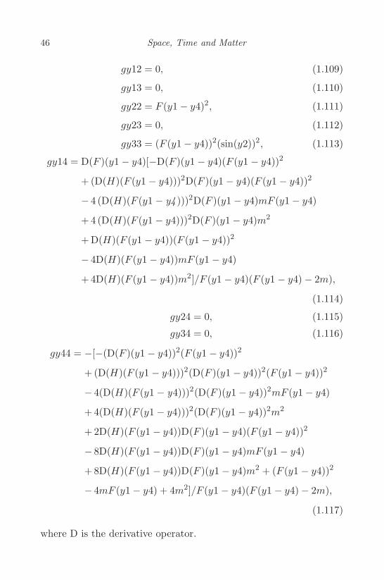
46 Space, Time and Matter
gy12 = 0, (1.109)
gy13 = 0, (1.110)
gy22 = F (y1− y4)2, (1.111)
gy23 = 0, (1.112)
gy33 = (F (y1− y4))2(sin(y2))2, (1.113)
gy14 = D(F )(y1 − y4)[−D(F )(y1 − y4)(F (y1 − y4))2
+ (D(H)(F (y1 − y4)))2D(F )(y1 − y4)(F (y1 − y4))2
− 4 (D(H)(F (y1 − y4 )))2D(F )(y1 − y4)mF (y1− y4)
+ 4 (D(H)(F (y1 − y4)))2D(F )(y1− y4)m2
+ D(H)(F (y1 − y4))(F (y1 − y4))2
− 4D(H)(F (y1 − y4))mF (y1 − y4)
+ 4D(H)(F (y1 − y4))m2]/F (y1 − y4)(F (y1 − y4)− 2m),
(1.114)
gy24 = 0, (1.115)
gy34 = 0, (1.116)
gy44 = −[−(D(F )(y1 − y4))2(F (y1 − y4))2
+ (D(H)(F (y1 − y4)))2(D(F )(y1 − y4))2(F (y1− y4))2
− 4(D(H)(F (y1 − y4)))2(D(F )(y1− y4))2mF (y1− y4)
+ 4(D(H)(F (y1 − y4)))2(D(F )(y1 − y4))2m2
+ 2D(H)(F (y1 − y4))D(F )(y1 − y4)(F (y1 − y4))2
− 8D(H)(F (y1 − y4))D(F )(y1 − y4)mF (y1 − y4)
+ 8D(H)(F (y1 − y4))D(F )(y1 − y4)m2 + (F (y1 − y4))2
− 4mF (y1− y4) + 4m2]/F (y1 − y4)(F (y1 − y4)− 2m),
(1.117)
where D is the derivative operator.
Space and Time 47
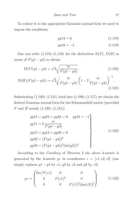
To reduce it to the appropriate Gaussian normal form we need to
impose the conditions
gy14 = 0, (1.118)
gy44 = −1. (1.119)
One can solve (1.118)–(1.119) for the derivatives D(F ), D(H) in
terms of F (y1− y4) to obtain
D(F )(y1 − y4) =√
2√
m
F (y1− y4), (1.120)
D(H)(F (y1 − y4)) =√
2√
m
F (y1− y4)
(1− 2
m
F (y1− y4)
)−1
.
(1.121)
Substituting (1.120)–(1.121) back into (1.108)–(1.117) we obtain the
desired Gaussian normal form for the Schwarzschild metric (provided
F and H satisfy (1.120)–(1.121))
gy14 = gy24 = gy34 = 0, gy44 = −1
gy11 = 2m
F (y1− y4)
gy12 = gy13 = gy23 = 0
gy22 = (F (y1 − y4))2
gy33 = (F (y1 − y4))2(sin(y2))2.
⎫⎪⎪⎪⎪⎪⎪⎪⎪⎪⎪⎬⎪⎪⎪⎪⎪⎪⎪⎪⎪⎪⎭(1.122)
According to the Corollary of Theorem 2 the above 4-metric is
generated by the 3-metric gz in coordinates z = [z1, z2, z3] (one
simply replaces y1− y4 by z1, y2 by z2 and y3 by z3)
gz =
⎛⎜⎜⎝2m/F (z1) 0 0
0 F (z1)2 0
0 0 F (z1)2(sin(z2))2
⎞⎟⎟⎠ (1.123)
48 Space, Time and Matter
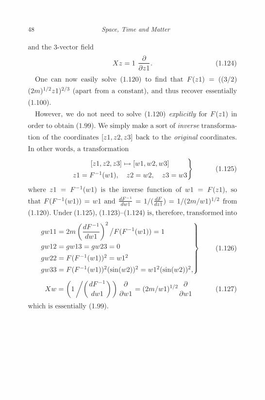
and the 3-vector field
Xz = 1∂
∂z1. (1.124)
One can now easily solve (1.120) to find that F (z1) = ((3/2)
(2m)1/2z1)2/3 (apart from a constant), and thus recover essentially
(1.100).
However, we do not need to solve (1.120) explicitly for F (z1) in
order to obtain (1.99). We simply make a sort of inverse transforma-
tion of the coordinates [z1, z2, z3] back to the original coordinates.
In other words, a transformation
[z1, z2, z3] �→ [w1, w2, w3]
z1 = F−1(w1), z2 = w2, z3 = w3
}(1.125)
where z1 = F−1(w1) is the inverse function of w1 = F (z1), so
that F (F−1(w1)) = w1 and dF−1
dw1 = 1/( dFdz1 ) = 1/(2m/w1)1/2 from
(1.120). Under (1.125), (1.123)–(1.124) is, therefore, transformed into
gw11 = 2m(
dF−1
dw1
)2 /F (F−1(w1)) = 1
gw12 = gw13 = gw23 = 0
gw22 = F (F−1(w1))2 = w12
gw33 = F (F−1(w1))2(sin(w2))2 = w12(sin(w2))2,
⎫⎪⎪⎪⎪⎪⎪⎬⎪⎪⎪⎪⎪⎪⎭(1.126)
Xw =(
1/(
dF−1
dw1
))∂
∂w1= (2m/w1)1/2 ∂
∂w1(1.127)
which is essentially (1.99).
Space and Time 49
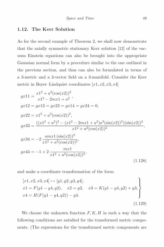
1.12. The Kerr Solution
As for the second example of Theorem 2, we shall now demonstrate
that the axially symmetric stationary Kerr solution [12] of the vac-
uum Einstein equations can also be brought into the appropriate
Gaussian normal form by a procedure similar to the one outlined in
the previous section, and thus can also be formulated in terms of
a 3-metric and a 3-vector field on a 3-manifold. Consider the Kerr
metric in Boyer–Lindquist coordinates [x1, x2, x3, x4]
gx11 =x12 + a2(cos(x2))2
x12 − 2mx1 + a2,
gx12 = gx13 = gx23 = gx14 = gx24 = 0,
gx22 = x12 + a2(cos(x2))2,
gx33 =((x12 + a2)2 − (x12 − 2mx1 + a2)a2(sin(x2))2)(sin(x2))2
x12 + a2(cos(x2))2,
gx34 = −2amx1 (sin(x2))2
x12 + a2(cos(x2))2,
gx44 = −1 + 2mx1
x12 + a2(cos(x2))2,
(1.128)
and make a coordinate transformation of the form:
[x1, x2, x3, x4] �→ [y1, y2, y3, y4],
x1 = F (y1− y4, y2), x2 = y2, x3 = K(y1− y4, y2) + y3,
x4 = H(F (y1− y4, y2)) − y4.
⎫⎪⎪⎬⎪⎪⎭(1.129)
We choose the unknown function F,K,H in such a way that the
following conditions are satisfied for the transformed metric compo-
nents. (The expressions for the transformed metric components are
50 Space, Time and Matter
too long to reproduce here. See Appendix D.)
gy14 = gy24 = gy34 = 0, gy44 = −1. (1.130)
These equations can now be solved for the following derivatives of
F,K,H, in terms of F (y1− y4) to give
D[1](F )(y1 − y4, y2)
=√
2√
m√
F (y1− y4, y2)a2 + (F (y1− y4, y2))3
(F (y1− y4, y2))2 + a2(cos(y2))2, (1.131)
D[1](K)(y1 − y4, y2)
= 2amF (y1− y4, y2)/[((F (y1 − y4, y2))2 + a2(cos(y2))2)
× ((F (y1 − y4, y2))2 − 2mF (y1− y4, y2) + a2)], (1.132)
D(H)(F (y1 − y4, y2))
=√
2√
m√
F (y1− y4, y2)a2 + (F (y1− y4, y2))3
(F (y1− y4, y2))2 − 2mF (y1− y4, y2) + a2. (1.133)
Here D[1](F ), D[1](K) are the first partial derivatives of F,K with
respect to the first argument y1 − y4, respectively. Note that there
are no conditions on the first partial derivatives of F,K with respect
to the second argument y2.
The above conditions (1.131)–(1.133) are not only necessary but
also sufficient for (1.130) to hold. In principle, therefore, one can solve
(1.131) for F (y1 − y4, y2) and, then, (1.132)–(1.133) to determine
K(y1− y4, y2), H(F (y1− y4, y2)). Unfortunately, (1.131) cannot be
integrated explicitly as it involves elliptic integrals.
Let us assume the above conditions (1.131)–(1.133). The compo-
nents of gy then have the appropriate Gaussian normal form given by
(1.105). They depend on functions of (y1−y4, y2) and y2 only. There-
fore, according to the Corollary of Theorem 2, gy is generated by the
Space and Time 51
3-metric gz in coordinates [z1, z2, z3] (where one replaces y1− y4 by
z1, y2 by z2 and y3 by z3 in gyik (i, k = 1, 2, 3) to get gzik) and the
3-vector field
Xz = 1∂
∂z1(1.134)
gzik (i, k = 1, 2, 3) contain only F (z1, z2), K(z1, z2) and their first
partial derivatives.
To obtain an explicit form of the 3-metric we make an “inverse”
transformation of the coordinates [z1, z2, z3] (analogous to the
Schwarzschild case) back to the “original” coordinates as follows:
[z1, z2, z3] �→ [w1, w2, w3]
z1 = F−1(w1, w2), z2 = w2,
z3 = w3−K(F−1(w1, w2), w2)
(1.135)
where F−1 is the inverse function of w1 = F (z1, z2) with respect to
the first variable, that is, F (F−1(w1, w2), w2) = w1.
Under (1.135) the vector field Xz is transformed into
Xw =[1/
∂F−1
∂w1(w1, w2)
]∂
∂w1
+ [D[1](K)(F−1(w1, w2), w2)]∂
∂w3. (1.136)
The transformed components gwik contain F (F−1(w1, w2), w2)
and only the following derivatives:
∂F−1
∂w1(w1, w2),
∂F−1
∂w2(w1, w2),
D[1](K)(F−1(w1, w2), w2),
D[1](F )(F−1(w1, w2), w2),
D[2](F )(F−1(w1, w2), w2).

52 Space, Time and Matter
These can be expressed explicitly in terms of w1, w2 as follows. From
(1.131) and (1.132), we have
F (F−1(w1, w2), w2) = w1, (1.137)
D[1](K)(F−1(w1, w2), w2)
=∂K
∂z1= 2
amw1(w12 + a2(cos(w2))2)(w12 + a2 − 2mw1)
,
(1.138)
∂F−1
∂w1(w1, w2)
= 1/
∂F
∂z1= 1/2
(w12 + a2(cos(w2))2)√
2√m√
w1(w12 + a2). (1.139)
Now, from (1.131), by integrating once
∂w1∂z1
=√
2√
m√
w1(w12 + a2)w12 + a2(cos(w2))2
,
we have
z1 =1
(2m)1/2
∫w12 + a2(cos(w2))2√
w1(w12 + a2)dw1,
apart from a function of w2, which we set equal to zero. Therefore,
∂z1∂w2
= −2a2 sin(w2) cos(w2)(2m)1/2
∫dw1√
w1(w12 + a2)
or
∂F−1
∂w2(w1, w2) = −2a2 sin(w2) cos(w2)
(2m)1/2EL(w1), (1.140)
where EL(w1) is a standard elliptic integral. And, again from (1.131),
D[1](F )(F−1(w1, w2), w2)
=∂F
∂z1=√
2√
m√
w1(w12 + a2)w12 + a2(cos(w2))2
. (1.141)
Space and Time 53
To calculate D[2](F )(F−1(w1, w2), w2) = ∂F∂z2 , we differentiate both
sides of (1.137) with respect to w2, to get
0 =∂w1∂w2
=∂F
∂z1∂F−1
∂w2(w1, w2) +
∂F
∂z2∂z2∂w2
=
[√2√
m√
w1(w12 + a2)w12 + a2(cos(w2))2
]
×[−a2 sin(w2) cos(w2)EL(w1)
√2√
m
]+
∂F
∂z2× 1
so that
D[2](F )(F−1(w1, w2), w2)
= 2a2 sin(w2) cos(w2)EL(w1)
√w1(w12 + a2)
w12 + a2(cos(w2))2. (1.142)
Finally, the explicit expressions for the 3-metric gw and the
3-vector field Xw, which generate the Kerr solution, are:
gw11 =w12 + a2(cos(w2))2
w12 + a2 − 2mw1
− 2mw1(w12 + a2)(w12 + a2(cos(w2))2 − 2mw1)
(w12 + a2(cos(w2))2)(w12 + a2 − 2mw1)2
(1.143)
gw12 = gw23 = 0, (1.144)
gw13 = −2a(sin(w2))2
√2m3/2w1
√w13 + a2w1
(w12 + a2(cos(w2))2)(w12 + a2 − 2mw1), (1.145)
gw22 = w12 + a2(cos(w2))2, (1.146)
gw33 =(
w12 + a2 − 2mw1 + 2mw1(w12 + a2)
w12 + a2(cos(w2))2
)(sin(w2))2,
(1.147)
54 Space, Time and Matter
Xw =
[√2√
m√
w13 + a2w1w12 + a2(cos(w2))2
]∂
∂w1
+[2
amw1(w12 + a2(cos(w2))2)(w12 + a2 − 2mw1)
]∂
∂w3.
(1.148)
One can now verify (Appendix E) that the above (g,X) is indeed
a solution of our Eqs. (1.41)–(1.43).
Note that, (1.143)–(1.145) reduce to the Schwarzschild case
(1.126)–(1.127) when a→ 0. When m→ 0, we obtain
gw =
⎡⎢⎢⎢⎢⎢⎢⎢⎢⎢⎣
w12 + a2(cos(w2))2
w12 + a20 0
0 w12 + a2 0
× (cos(w2))2
0 0 (w12 + a2)
× (sin(w2))2
⎤⎥⎥⎥⎥⎥⎥⎥⎥⎥⎦,
(1.149)
Xw = 0. (1.150)
The above 3-metric (1.149) is flat, and therefore (1.149)–(1.150) is
equivalent to the flat space-time.
If a = 0, the 3-metric (1.143)–(1.145) is not flat, in contrast to
(1.126), the 3-metric in the Schwarzschild case. Its scalar curvature
is given by
Rw =2a2mw1(3(cos(w2))2 − 1)
w12 + a2(cos(w2))2(1.151)
and the 3-vector field Xw in (1.148) has the length
g(X,X) = gw(Xw,Xw) =2mw1
w12 + a2(cos(w2))2. (1.152)

Space and Time 55
Thus X ceases to be “physical” when g(X,X) = 1, i.e.,
2mw1w12 + a2(cos(w2))2
= 1 (1.153)
which corresponds to the so-called stationary limit of the Kerr
black hole.
56 Space, Time and Matter
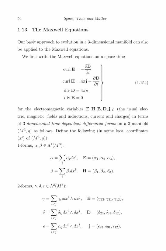
1.13. The Maxwell Equations
Our basic approach to evolution in a 3-dimensional manifold can also
be applied to the Maxwell equations.
We first write the Maxwell equations on a space-time
curl E = −∂B∂t
curl H = 4πj +∂D∂t
div D = 4πρ
div B = 0
⎫⎪⎪⎪⎪⎪⎪⎪⎪⎬⎪⎪⎪⎪⎪⎪⎪⎪⎭(1.154)
for the electromagnetic variables E,H,B,D, j, ρ (the usual elec-
tric, magnetic, fields and inductions, current and charges) in terms
of 3-dimensional time-dependent differential forms on a 3-manifold
(M3, g) as follows. Define the following (in some local coordinates
(xi) of (M3, g)):
1-forms, α, β ∈ Λ1(M3):
α =∑
i
αidxi, E = (α1, α2, α3),
β =∑
i
βidxi, H = (β1, β2, β3).
2-forms, γ, δ, ε ∈ Λ2(M3):
γ =∑i<j
γijdxi ∧ dxj, B = (γ23, γ31, γ12),
δ =∑i<j
δijdxi ∧ dxj , D = (δ23, δ31, δ12),
ε =∑i<j
εijdxi ∧ dxj , j = (ε23, ε31, ε12).

Space and Time 57
3-form: η ∈ Λ3(M3):
η = ρ dx1 ∧ dx2 ∧ dx3.
Note that these 3-dimensional forms are time-dependent with the
time t as a parameter. Using the exterior derivative operator d the
Maxwell equations (1.154) can then be written as:
dα = −∂γ
∂t
dβ = 4πε +∂δ
∂t
dδ = 4πη
dγ = 0.
⎫⎪⎪⎪⎪⎪⎪⎪⎬⎪⎪⎪⎪⎪⎪⎪⎭(1.155)
As we did in the case of Gauss–Einstein equations, let us now
replace the time-derivative ∂∂t in (1.155) by the Lie-derivative LX
with respect to some vector field X on M3. Then (1.155) becomes
dα = −LXγ, (1.156)
dβ = 4πε + LXδ, (1.157)
dδ = 4πη, (1.158)
dγ = 0. (1.159)
Here, α, β, γ, δ, ε, η are to be regarded now as (time-independent)
purely 3-dimensional differential forms on M3. Equations (1.156)–
(1.159) are thus analogous to (1.38)–(1.40), corresponding to the
Gauss–Einstein equations, and are to be considered as a set of equa-
tions for the forms α, β, γ, δ, ε, η and the vector field X. Every solu-
tion of (1.156)–(1.159) determines uniquely a solution of (1.155) and,
thus, of (1.154).e One simply has to transform the time-independent
eAgain, the converse need not be true.
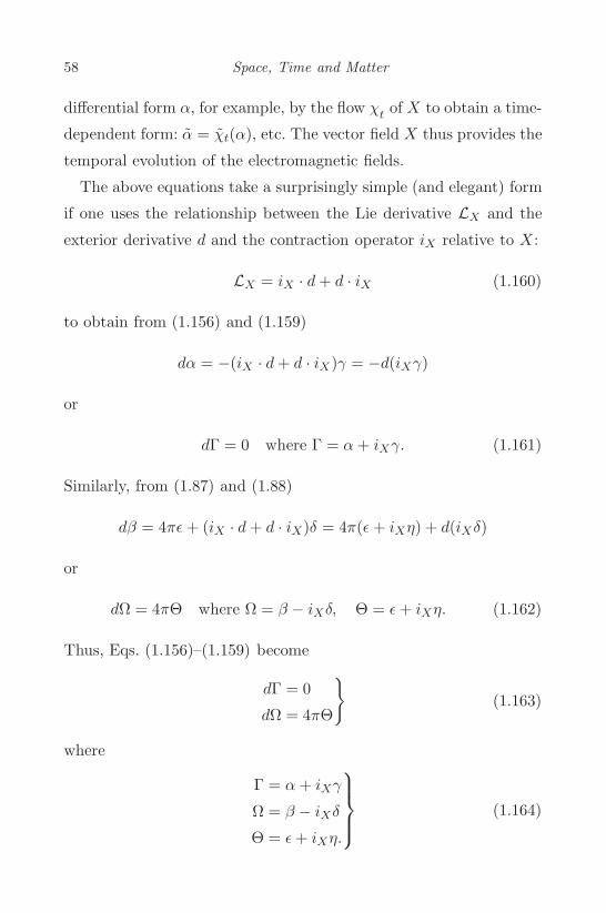
58 Space, Time and Matter
differential form α, for example, by the flow χt of X to obtain a time-
dependent form: α = χt(α), etc. The vector field X thus provides the
temporal evolution of the electromagnetic fields.
The above equations take a surprisingly simple (and elegant) form
if one uses the relationship between the Lie derivative LX and the
exterior derivative d and the contraction operator iX relative to X:
LX = iX · d + d · iX (1.160)
to obtain from (1.156) and (1.159)
dα = −(iX · d + d · iX)γ = −d(iXγ)
or
dΓ = 0 where Γ = α + iXγ. (1.161)
Similarly, from (1.87) and (1.88)
dβ = 4πε + (iX · d + d · iX)δ = 4π(ε + iXη) + d(iXδ)
or
dΩ = 4πΘ where Ω = β − iXδ, Θ = ε + iXη. (1.162)
Thus, Eqs. (1.156)–(1.159) become
dΓ = 0
dΩ = 4πΘ
}(1.163)
where
Γ = α + iXγ
Ω = β − iXδ
Θ = ε + iXη.
⎫⎪⎪⎬⎪⎪⎭ (1.164)
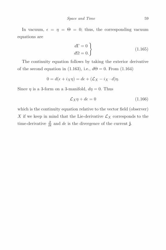
Space and Time 59
In vacuum, ε = η = Θ = 0; thus, the corresponding vacuum
equations are
dΓ = 0
dΩ = 0.
}(1.165)
The continuity equation follows by taking the exterior derivative
of the second equation in (1.163), i.e., dΘ = 0. From (1.164)
0 = d(ε + iXη) = dε + (LX − iX · d)η.
Since η is a 3-form on a 3-manifold, dη = 0. Thus
LXη + dε = 0 (1.166)
which is the continuity equation relative to the vector field (observer)
X if we keep in mind that the Lie-derivative LX corresponds to the
time-derivative ∂∂t and dε is the divergence of the current j.

60 Space, Time and Matter
References
[1] G. D. Mostow, Strong Rigidity of Locally Symmetric Spaces, Ann.
Math. Series (Princeton Univ. Press, Princeton, 1973).
[2] S. Helgason, Differential Geometry and Symmetric Spaces (Academic,
New York, 1972).
[3] S. Kobayashi and K. Nomizu, Foundations of Differential Geometry,
Vol. 1 (Interscience, New York, 1983).
[4] D. V. Widder, The Heat Equation (Academic Press, New York, 1975).
[5] A. Lichnerowicz, Theories relativistes de la gravitation et de
l’electromagnetisme (Masson, Paris, 1955).
[6] J. S. Synge, Relativity, the General Theory (North-Holland, Amster-
dam, 1960).
[7] A. E. Fisher and J. E. Marsden, J. Math. Phys. 13 (1972) 546–568.
[8] E. Kasner, American J. Math. 43 (1921) 217.
[9] G. Lemaitre, L’univers en expansion, Ann. Soc. Sci. Bruxelles I A 53
(1933) 51.
[10] A. Z. Petrov, Einstein Spaces (Pergamon Press, Oxford, 1969).
[11] D. K. Sen, Class. Quant. Gravity 12 (1995) 553–577.
[12] D. K. Sen, J. Math. Phys. 41 (2000) 7556–7572.