Sources of experimental variation in calibration curves for enzyme-linked immunosorbent assay

ANALYTIcA CHIMICA ACM

Analytica Chimica Acta 313 (1995) 197-207 ELSEVIER

Sources of experimental variation in calibration curves for enzyme-linked immunosorbent assay

Geoffrey Jones a, Monika Wortberg b, Sabine B. Kreissig b, Bruce D. Hammock b, David M. Rocke a, *

a Graduate School of Management, University of California, Davis, CA 95616, USA

b Departments of Entomology and Environmental Toxicology, University of California, Dauis. CA 95616. USA

Received 30 January 1995; revised 1 May 1995; accepted 9 May 1995

Abstract

Enzyme-linked immunosorbent assays are usually performed by running standard and unknown concentrations together on the same microtiter plate, because the standard curve is known to vary considerably from one assay to the next. Here we examine experimentally the sources and nature of this variation, and discuss the possibility of reducing the cost of the assay by using a batch of plates, only one of which is used to generate the calibration curve. We present a method for doing this,

and test it empirically.

Keywords: Immunoassay; Calibration; Enzymatic methods; ELISA

1. Introduction

Enzyme-linked immunosorbent assays (ELISAs) are rapid and sensitive methods for quantitating clin-

ical or environmental analytes in trace amounts [l-7]. The assay is typically run on a 96-well microtiter plate, with some cells reserved for the generation of a calibration curve using known standard concentrations, the remaining cells being used for the unknown samples (Fig. 1). Responses (in the form of optical densities) from the unknowns are then trans-

’ Corresponding author

formed via the calibration curve into estimated con-

centrations. Typically, the calibration curve obtained is sig-

moidal in shape, and a number of different curve-fit- ting and estimation procedures have been developed: from non-parametric smoothing techniques, through

the use of empirical mathematical models, to theoret- ical models based on the mass-action law [8].

The four-parameter log-logistic model:

A-D Y= x B+D

i 1

(1)

1+ c

where y is the ELISA response (optical density), x the analyte concentration, A and D the responses at zero and infinite dose, C the IC50 (the concentration

0003.2670/95/$09.50 0 1995 Elsevier Science B.V. AI1 rights reserved

SSDI 0003-2670(95)00249-9

198 G. Jones ef al. /Analytica Chimica Acta 313 (1995) 197-207

(a) Single analyte

saPpies

(b) Multi-analyte

samp es

Fig. 1. Typical ELBA templates.

giving 50% inhibition) and B a slope parameter, has been shown to be a useful and flexible tool in

assaying the concentration of a single analyte for a variety of ELISA formats [9-111, and to be prefer- able to the mass-action model in many situations [12,13].

The parameters of the log-logistic model are

known to be subject to considerable experimental variation, so it is usually deemed necessary to evaluate separate calibration curves for each microplate. Since space on each plate has therefore to be allo- cated to standard known concentrations, this limits the number of unknown samples to be included and increases the cost of the assay, a consideration of particular importance in the environmental field where the speed, low cost and parallel nature of the assay make it especially suitable for large monitoring programs. In the case of multi-analyte determination for cross-reacting analytes [14-161 this limitation can be severe (see Fig. lb).

The question naturally arises, therefore, as to whether some or all of the parameters could be ‘borrowed’ from previously generated standard

curves, or from curves generated on the same day in the same laboratory, or from curves generated on

other plates treated simultaneously with plates of unknowns. Clearly the important criterion, as ever,

will be the accuracy of calibration of unknown samples: the parameter values themselves are only inter-

mediaries in the calibration process. Nevertheless a

study of the way in which the curves vary from day to day, from lab to lab, and from plate to plate,

should give some indication as to which of the above suggestions, if any, is reasonable. It is known that the relationship between response and analyte concentration can vary significantly from one location to

another on the same plate [17]: if the variation between curves on different plates is no greater than this, there is nothing to be lost by borrowing the

curve, or some of its parameters, from another plate. Our approach to studying the variation in the

curves clearly depends on the particular parameteri-

zation used, which could be regarded as arbitrary. We would argue, however, that the parameters have a natural interpretation which makes them worthy of study: A and D relate to the maximum and mini- mum amount of bound antibody, which in turn de- pend on the adsorptive properties of the plate; B and

C should be characteristic of the bonding reaction itself, and so might not be expected to vary signifi-

cantly from plate to plate. The aim of this paper then is to examine experi-

mentally some possible factors which could cause variation in the parameters A, B, C and D, and to

estimate their relative importance. In particular we are interested in the stability of the parameters from plate to plate when other factors are held constant.

Our results suggest a method for running additional plates without the need to re-evaluate complete standard curves: since plate-to-plate variation in B and C is found to be non-significant compared to variation

within plates, these parameters can be estimated on one plate per batch; the A and D parameters, which do exhibit significant plate-to-plate variation, can then be estimated for each additional plate using zeros and blanks only.

We then test the method empirically by examin- ing the accuracy of calibration of unknowns, for both single-analyte and multi-analyte ELISA, and compare our suggested method with a more simplistic approach in which A and D are not re-estimated.

G. Jones et al./Analytica Chimica Acta 313 (1995) 197-207 199

2. Experimental

2.1. Design of study

There are many possible factors which might

affect the complex immunochemical reaction taking place in each cell of the microtiter plate, and thereby

the estimated curve parameters: external physical conditions, particularly temperature, variations in ex-

perimental procedure, differences in the adsorptive properties of different plates, or of different locations on the same plate, variations between batches of

stock solutions. Some of these are beyond the normal control of the experimenter. In choosing the factors

for our experiment, we need a partition of the sources of variation which will have practical relevance for the technician. The following factors were identified and used in the study:

DAY, assays were run on two different days one

week apart; LAB, assays were performed each day in two

different laboratories by different technicians; TIME, two incubation times were used for the

substrate conversion step: 20 min and 40 min;

PLATE, two plates were run for each possible combination of the above factors;

LOCATION, each plate was divided into four equal sections, each containing a set of standards for the estimation of a calibration curve.

In addition two different antibodies were used,

both reactive to the analyte but one monoclonal and

the other polyclonal; the data for each antibody were analyzed separately and compared. Thus a total of 32 plates was run over two days, giving 64 sets of estimated A, B, C and D parameters for each antibody. The same stock solutions were used

throughout, and a common dilution series, to be used by both laboratories, was prepared on each day. All microtiter plates used were from the same manufac- turer.

It was decided to exclude data where the curves were suspect or where there were outlying points: from a practical viewpoint such assays would pre- sumably be rejected by a technician, and theoreti- cally they would lead to an inflated error variance and cause problems in the analysis of our experiment.

All factors except TIME are regarded as random

TIME

TIME

DAY 2

Fig. 2. Design of components of variance experiment.

effects: an incubation time of, say, 20 min can be chosen by the technician, and might be supposed to give a consistent effect, whereas conditions vary

from lab to lab and from day to day. The design uses a nesting structure as shown in Fig. 2; thus LAB is

nested in DAY since the LAB effect may vary from day to day, whereas TIME is crossed with LAB since the same incubation time is used in each

laboratory. Since LOCATION effects cannot be sep- arated from pure replication error, LOCATION is not included as a factor in the analysis; thus the residual variation between curves is attributable in part to location effects on the plates.

Analysis of the results from this experiment suggested a methodology which was tested in two fur- ther assay systems as described below.

2.2. Materials

The monoclonal antibody AM7B2.1 was kindly donated by A. Karu (University of California, Berke- ley, CA) [18], KlF4 was provided by B. Hock and T. Giersch (TU Muenchen-Weihenstephan, Germany)

[19]. The polyclonal antibody 842 was produced by Harrison et al. [20], the polyclonal 2266 by Lucas et al. [21]. The triazine herbicide derivatives were syn- thesized by Goodrow [22]. Triazine herbicide standards were from Ciba-Geigy (Greensboro, NC). Horseradish peroxidase (HRP) conjugates of anti- mouse IgG and anti-rabbit IgG as well as ovalbumin grade VI, crude ovalbumin, l-ethyl-3-(3-dimethyl- aminopropyl) carbodiimide, and tetramethylbenzi- dine (TMB) were purchased from Sigma. Dimethyl- formamide (DMF) of LC grade and N-hydroxysuc-

200 G. Jones et al./Analytica Chimica Acta 313 (1995) 197-207

cinimide (NHS) were obtained from Aldrich (Milwaukee, WI). Buffer reagents of analytical grade were purchased from Fisher (Fair Lawn, NJ). For purification of ovalbumin-hapten conjugates we used lo-ml Presto desalting columns (Pierce, Rockford, IL). Microtiter plates were obtained from Nunc (Denmark). For reading the optical densities we used a Molecular Devices UVMax Reader equipped with standard ELISA software.

systems used (for the original investigation and two confirmatory experiments) were:

System I: atrazine calibration curves using the two antibodies AM7B2.1 and 842;

System II: atrazine calibration curves with spiked samples on the same and on separate plates, demon- strated with AM7B2.1;

2.3. ELISA format

System III: ternary triazine mixture analysis using atrazine, hydroxyatrazine and prometryne calibration curves with spiked samples on the same and on separate plates, and three antibodies: AM7B2.1, KlF4 and 2266 (following Kreissig et al. [16]).

For both single analyte and multianalyte ELISA For the two different triazine derivatives to be we used a coating hapten format. The competitive used as coating haptens with the antibodies KlF4, type assay comprised 3 steps: competitive incubation AM7B2.1 and 2266 the coupling technique chosen of standard or spiked sample together with the spe- was the active ester method [23]. Coupling com- cific antibody, introduction of a secondary HRP prised transforming the acid functional group on the labeled antibody and conversion of the enzyme sub- triazine derivatives in an N-hydroxy succinimide strate TMB into a colored product. The three assay ester using EDC and subsequent reaction with the

[ AM7B #842 l 0.05 l -4

l e 0

l l

l 8 0 00 0

1.4

1.2

0

g 1.0

5 2 p 0.8

0.6

3.4 0.6 0.8 1.0 1.2

Parameter A

AM7B l

0.9 1.0 1.1 1.2 1.3

Parameter I3

0.08

n

$0.06

E

a” 0.04

0.02

1.4

1.2

0.6

“0% 0

0.2 0.4 0.6 0.8

Parameter A

#842 0 0 A

0.7 0.8 0.9 1.0 1.1 1.2 1.3

Parameter B

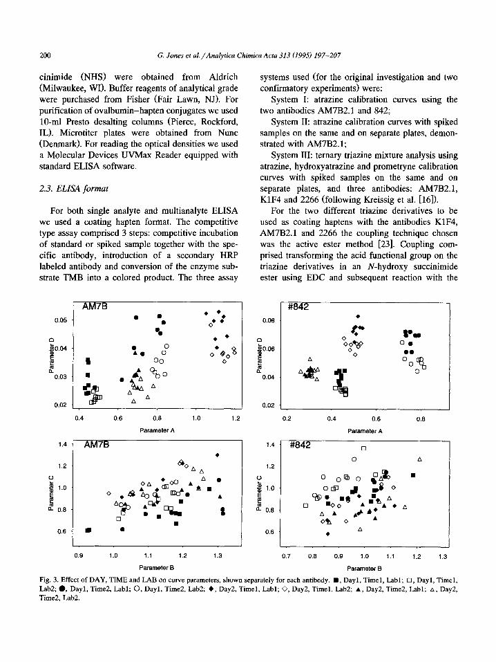
Fig. 3. Effect of DAY, TIME and LAEI on curve parameters, shown separately for each antibody. n , Dayl, Timel, Labl; 0, Dayl, Timel,

Lab2; 0, Dayl, Time2, Labl; 0, Dayl, Time2, Lab2; +, Day2, Timel, Labl; 0, Day2, Timel, Lab2; A, Day2, Time2, Labl; A, Day2, Time2, Lab2.

G. Jones et al. /Analytica Chimica Acta 313 (19951 197-207 201

protein ovalbumin. A more reactive sulfoxide func-

tionalized triazine derivative which was used in combination with antibody 842 was coupled to the protein without addition of activating agents. The cou-

pling is described in more detail in [15]. For plate coating, hapten-ovalbumin conjugates

were diluted 1:lO 000 in 0.1 M phosphate buffered saline (PBS) buffer. 175 ~1 per well was incubated overnight at 4°C. Subsequently, the wells were emp- tied and incubated with 175 ~1 of a 0.5% (w/v) solution of crude ovalbumin in PBS for 1 h. After

washing the wells four times with 0.01 M PBS

containing 0.05% Tween 20 (washing buffer) the

plates were ready to use for the assay systems I-III. For single and multianalyte analysis, triazine stan-

dards were either assayed together with the triazine mixtures on the same plate or on separate plates. For

multianalyte analysis, the same standards and/or samples were run three times on three different

plates, each using a different antibody-coating hapten combination.

In the competitive step, 100 ~1 triazine standard or sample were pipetted into the wells. Standards were diluted in PBS from 1 mg/ml DMF stock

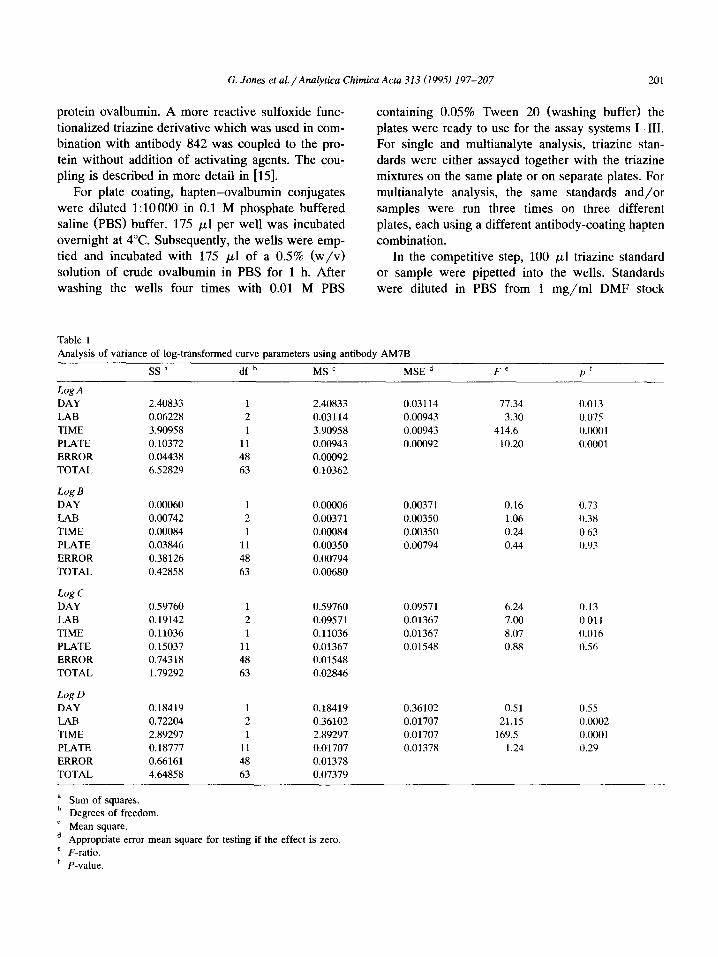
Table I Analysis of variance of log-transformed curve parameters using antibody AM7B

ss a df b MS ’ MSE d Fe Pf

LogA

DAY LAB TIME PLATE ERROR TOTAL

LogB


Log c


LogD


2.40833 1 2.40833 0.06228 2 0.03114 3.90958 1 3.90958 0.10372 11 0.00943 0.04438 48 0.00092 6.52829 63 0.10362

0.00060 1 0.00006 0.00742 2 0.00371 0.00084 1 0.00084 0.03846 11 0.00350 0.38126 48 0.00794 0.42858 63 0.00680

0.59760 1 0.59760 0.19142 2 0.09571 0.11036 1 0.11036 0.15037 11 0.01367 0.74318 48 0.01548 1.79292 63 0.02846

0.18419 1 0.18419 0.72204 2 0.36102 2.89297 1 2.89297 0.18777 11 0.01707 0.66161 48 0.01378 4.64858 63 0.07379

0.03114 77.34 0.013 0.00943 3.30 0.075 0.00943 414.6 0.0001 0.00092 10.20 0.0001

0.0037 1 0.16 0.73 0.00350 1.06 0.38 0.00350 0.24 0.63 0.00794 0.44 0.93

0.09571 6.24 0.13 0.01367 7.00 0.011 0.01367 8.07 0.016 0.01548 0.88 0.56

0.36102 0.51 0.55 0.01707 21.15 0.0002 0.01707 169.5 0.0001 0.01378 1.24 0.29

6 Sum of squares. Degrees of freedom.

’ Mean square. d Appropriate error mean square for testing if the effect is zero. ’ F-ratio. ’ P-value.

202 G. Jones et al. /Analytica Chimica Acta 313 (1995) 197-207

solutions. Then 50 ~1 of the respective antibody diluted in PBS was added. The dilution factors of the

antibodies were: 842, 1:2000; 2266, 1:5000; KlF4

(ascites), 1:8000; and AM7B2.1 (cell culture), 1500. After 1 h of competition the wells were rinsed four times with washing buffer. The secondary antibody HRP conjugates were diluted 1:8000 (anti-mouse) and 1:15 000 (anti-rabbit) respectively. A lOO-~1

aliquot of the labeled antibody was incubated for 1 h, then the wells were again rinsed 4 times. The sub-

strate solution was prepared by mixing 400 ~1 of a 6 mg/ml TMB stock solution (in DMSO) and 100 ~1

1% H,O, per 25 ml 0.1 M sodium acetate buffer pH 5.5. A loo-p1 aliquot of this substrate solution was allowed to react for exactly 20 or 40 min for the assay system I or 15-45 min for the systems I and

III, then the reaction was stopped by adding 50 ~1 of

2 M H,SO,. Plates were read at 450 nm in the ELISA reader, using a 650 nm background correc-

tion. Curves were fitted using a non-linear minimiza-

tion routine 1241, assuming a constant coefficient of variation for the response-error relationship [25].

2.4. Assay system I (32 plates)

For this assay the plates were divided into four

columns of 3 X 8 wells each. Four standard curves were run on the same plate using concentrations of 0,

0.1, 0.3, 1, 3, 10, 100 and 10000 ppb atrazine in triplicates. The template was the same for all plates, each being divided into four 8 X 4 sections. Half of the plates were run by one operator in one lab, the

other half by a second operator in another lab (as described in Section 2.1). Each operator dedicated

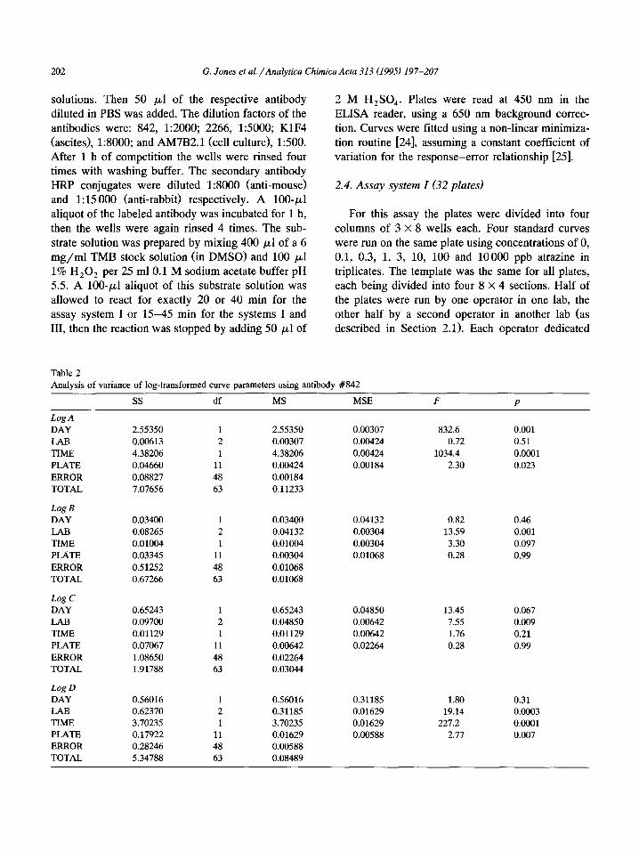
Table 2 Analysis of variance of log-transformed curve parameters using antibody #842

SS df MS MSE F P

LogA


Log B


Log c


Log D


2.55350 1 2.55350 0.00613 2 0.00307 4.38206 1 4.38206 0.04660 11 0.00424 0.08827 48 0.00184 7.07656 63 0.11233

0.03400 1 0.03400 0.08265 2 0.04132 0.01004 1 0.01004 0.03345 11 0.00304 0.51252 48 0.01068 0.67266 63 0.01068

0.65243 1 0.65243 0.09700 2 0.04850 0.01129 1 0.01129 0.07067 11 0.00642 1.08650 48 0.02264 1.91788 63 0.03044

0.56016 1 0.56016 0.62370 2 0.31185 3.70235 1 3.70235 0.17922 11 0.01629 0.28246 48 0.00588 5.34788 63 0.08489

0.00307 832.6 0.001 0.00424 0.72 0.51 0.00424 1034.4 0.0001 0.00184 2.30 0.023

0.04132 0.82 0.46 0.00304 13.59 0.001 0.00304 3.30 0.097 0.01068 0.28 0.99

0.04850 13.45 0.067 0.00642 7.55 0.009 0.00642 1.76 0.21 0.02264 0.28 0.99

0.31185 1.80 0.31 0.01629 19.14 0.0003 0.01629 227.2 0.0001 0.00588 2.77 0.007

G. Jones et al./Analytica Chimica Acta 313 (19951 197-207 LO3

half the total number of plates to each antibody. The coating hapten solution, antibody dilutions and atra-

zine standards were prepared from the same stock solution prior to each experiment and then split. Thus, both operators used the same solutions. Incu- bation times were monitored strictly using a stop

watch, with particular emphasis put on the timing of the substrate conversion step.

2.5. Assay system II (2 plates)

This assay was designed to compare the accuracy

of analysis of samples on the same plate as the

standard curves with that of samples on additional plates with borrowed curve parameters. Thus one

plate contained a set of standard atrazine concentrations for calibration and two sets of 6 spiked samples: the second plate contained three sets of the samples together with zeros and blanks. All samples

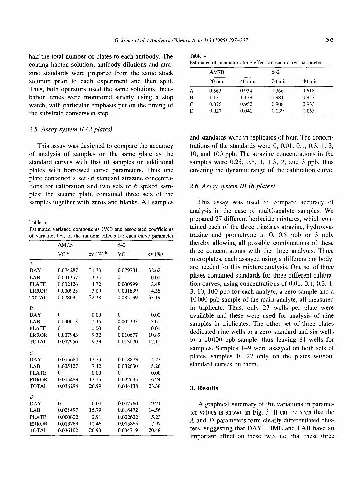
Table 3

Estimated variance components (VC) and associated coefficients

of variation (cv) of the random effects for each curve parameter

Awl3 842

vc a cv(%) b vc cv (%I

A

DAY

LAB

PLATE

ERROR

TOTAL

B

DAY

LAB

PLATE

ERROR

TOTAL

c

DAY

LAB

PLATE

ERROR

TOTAL

D

DAY LAB

PLATE

ERROR

TOTAL

0.074287 31.33

0.001357 3.15

0.002126 4.72

0.000925 3.09

0.078695 32.38

0.079701

0

0.000599

0.001839

32.62

0.00

2.48

4.38

33.19

0 0.00 0 0.00

0.000013 0.36 0.002393 5.01

0 0.00 0 0.00

0.007943 9.32 0.010677 10.89

0.007956 9.33 0.013070 12.11

0.015684 13.34 0.018873 14.73

0.005127 7.42 0.002630 5.26

0 0.00 0 0.00

0.015483 13.25 0.022635 16.24

0.036294 20.99 0.044138 23.38

0 0.00 0.007760 9.21 0.021497 15.79 0.018472 14.56

0.000822 2.91 0.002602 5.23

0.013783 12.46 0.005885 7.97

0.036102 20.93 0.034719 20.48

Table 4

Estimates of incubation time effect on each curve parameter

Ah47B 842

20 min 40 min 20 min 40 min

A 0.563 0.934 0.366 0.618

B 1.131 1.139 0.98 1 0.957

C 0.876 0.952 0.908 0.933

D 0.027 0.041 0.039 0.063

and standards were in replicates of four. The concen-

trations of the standards were 0, 0.01, 0.1, 0.3, 1. 3, 10, and 100 ppb. The atrazine concentrations in the

samples were 0.25, 0.5, 1, 1.5, 2, and 3 ppb, thus

covering the dynamic range of the calibration curve.

2.6. Assay system III (6 plates)

This assay was used to compare accuracy of

analysis in the case of multi-analyte samples. We prepared 27 different herbicide mixtures, which contained each of the three triazines atrazine, hydroxya-

trazine and prometryne at 0, 0.5 ppb or 3 ppb, thereby allowing all possible combinations of these three concentrations with the three analytes. Three

microplates, each assayed using a different antibody, are needed for this mixture analysis. One set of three

plates contained standards for three different calibration curves, using concentrations of 0.01, 0.1, 0.3, 1, 3, 10, 100 ppb for each analyte, a zero sample and a 10 000 ppb sample of the main analyte, all measured in triplicate. Thus, only 27 wells per plate were available and these were used for analysis of nine

samples in triplicates. The other set of three plates dedicated nine wells to a zero standard and six wells to a 10000 ppb sample, thus leaving 81 wells for samples. Samples l-9 were assayed on both sets of

plates, samples lo-27 only on the plates without standard curves on them.

3. Results

A graphical summary of the variations in parameter values is shown in Fig. 3. It can be seen that the A and D parameters form clearly differentiated clus- ters, suggesting that DAY, TIME and LAB have an important effect on these two, i.e. that these three

204 G. Jones et al./Analytica Chimica Acta 313 (1995) 197-207

Table 5

Recovery of atraxine in spiked samples. Amounts Sl, S2 are from samples on the same plate as the standard curve, Al-A3 on an additional

plate with the A and D parameters re-estimated from zeros and blanks, Al’ -A3 l on the additional plate but without adjustment

True Standard Additional (adj.) Additional (unadj.)

cont.

(ppb) Sl s2 Al A2 A3 Al’ A2’ A3’

0.25 0.43 0.35 0.39 0.47 0.47 0.34 0.41 0.42

0.50 0.58 0.55 0.70 0.71 0.69 0.63 0.62 0.62

1.00 1.09 1.10 1.07 1.25 1.20 0.96 1.07 1.07

1.50 1.42 1.53 1.56 1.75 1.66 1.38 1.46 1.46

2.00 2.00 1.94 1.93 2.02 2.04 1.68 1.77 1.77

3.00 2.84 2.65 2.77 2.79 2.63 2.33 2.23 2.23

factors account for much of the observed variation in

A and D. Conversely there is no such pattern dis- cernible from inspection of the B and C plots.

2.5

Determined 2 concentration

(Ppb) 1.5

1

0.5

0” I I I ” I 0 0.5 1 1.5 2 2.5 3 3.5

Actual concentration (ppb)

3.5

3

2.5

Determined 2 concentmtion

(PPb) 1.5

1

0.5

0” 0 0.5 1 1.5 2 2.5 3 3.5

Actual concentration (ppb)

Sl S2 Al*APA3’ 8ft - -* -*

Fig. 4. Correlation plot of amount of atraxine recovered against

amount added in the single-analyte confirmatory experiment, with

(a) and without (b) adjustment of the A and D parameters.

Samples Sl, S2 were on the same plate as the standard curve;

Al-A3 were on an additional plate without a standard curve. The

lines show the best linear fit for each set of points.

However, B and C do appear to be approximately linearly related, with the linear relationship changing

slightly for each different combination of factors. We now proceed to a statistical analysis of the variations.

3.1. Statistical analysis

Mixed model analysis of variance [26] for each of the four parameters was carried out using the GLM procedure in SAS [27]. The results are given in

Tables 1 and 2. The raw parameter values were transformed by taking logarithms: as well as being intuitively reasonable (corresponding to constant cv, or proportional errors in the parameter estimates),

this gave residuals which showed no obvious depar- ture from the assumptions of Gaussian errors and homoscedasticity required for the use of F-tests. The

DAY-TIME and LAB-TIME interactions were originally included in the analysis, but were subsequently omitted as these effects were found to be small and mostly non-significant.

Estimated variance components and associated cv’s for the random effects were calculated from the ANOVA output (see Table 3). When the appropriate error mean square exceeded the effect mean square, the corresponding variance component was taken as zero. The cv’s here represent estimates of the result- ing cv of the actual parameter value if the corresponding factor could be allowed to vary with all other factors kept fixed. The estimated TIME effects are given in Table 4.

3.2. Conclusions

It can be seen that all four parameters vary considerably between different locations on the same

G. Jones et al./Anolytica Chimica Acta 313 11995) 197-207 205

Table 6

Linear regression analysis of amount of atrazine found on amount added, showing the coefficient of determination (R’), intercept (a) and

slope (b) of the least squares line, with standard errors in brackets

Standard Additional (adj.) Additional (unadj.)

Sl s2 Al A2 A3 Al* AZ’ A3’

R2 (‘S/o) 99.1 99.3 99.8 US.9 98.6 99.4 98.1 97.9

u 0.17 (0.04) 0.19 (0.06) 0.23 (0.03) 0.34 (0.07) 0.35 (0.08) 0.24 (0.04) 0.34 (0.08) 0.34 (0.08)

h 0.89 (0.03) 0.85 (0.03) 0.85 (0.02) 0.84 (0.04) 0.80 (0.05) 0.71 (0.02) 0.70 (0.05) 0.67 (0.05)

plate: in fact this seems to be the most important source of variation for the B and C values. Of particular importance is the finding that B and C do not vary significantly from plate to plate, so that

observed variation in these parameters between plates is not greater than between different locations on the

same plate. Thus it would seem that putting the standard calibration concentrations on the same plate as the unknowns might not lead to significantly better estimates than having them on a separate plate, provided that both plates receive identical treatment

under the same conditions. The A and D parameters, representing the upper

and lower horizontal asymptotes to the calibration curve, do however seem to vary significantly from plate to plate, but these can be estimated from zero

concentrations and blanks (infinite concentrations), respectively. We therefore propose running additional plates devoted almost entirely to unknowns, with a few cells used for the re-estimation of the A

and D parameters; the additional plates should be run at the same time as the standard plate, under the same experimental conditions.

3.3. Confirmatory experiment - single analyte

Table 5 shows the true atrazine concentrations in the six spiked samples together with the amounts recovered: Sl and S2 are the estimates from the two sets of samples on the standards plate; Al, A2, A3 were estimated from the three sets of samples on the additional plate using the B and C parameters from

the standards plate but A and D re-estimated from the zeros and blanks on the additional plate; Al*, A2*, A3’ are as for Al, A2, A3 but using all the standards plate parameters (i.e. without adjusting for a different A and 0).

Regression of amount found on amount added is shown in Fig. 4 and Table 6. It appears from these

results that reasonable estimations can be achieved

Table 7

Simultaneous recovery of atrazine, prometryne and OH-atrazine in multi-analyte analysis, for samples either on the standard plate or on an

additional plate with and without adjusting for re-estimated A and D

True cont. (ppb) Standard Additional (adj.) Additional (unadj.)

Atrazine Prometryne OH- Atrazine Prometryne OH- Atrazine Prometryne OH- Atrazine Prometryne OH-

atrazine atrazine atrazine atrazine

0 0

0 0.5

0 3

0.5 0

0.5 0.5

0.5 3

3 0

3 0.5

3 3

0 0.00 0.00 0.00 0.00 0.00 0.01 0.00 0.00 0.01

3 0.00 0.41 2.15 0.04 0.36 1.99 0.00 0.49 I .83

0.5 0.00 3.43 0.29 0.14 3.02 0.27 0.00 3.39 0.27

3 0.38 0.16 2.58 0.53 0.00 1.94 0.34 0.19 I .oo 0.5 0.60 0.41 0.40 0.63 0.19 0.33 0.4 I 0.41 0.33

0 0.42 2.77 0.00 0.60 2.75 0.00 0.27 3.29 0.00

0.5 2.69 0.49 0.28 2.83 0.29 0.41 2.41 066 0.41

0 2.59 1.13 0.00 2.98 0.68 0.00 2.54 1.09 O.00

3 2.38 3.38 2.57 2.94 3.31 2.59 2.32 3.38 2.57

206 G. Jones et al. /Analytica Chimica Acta 313 (1995) 197-207

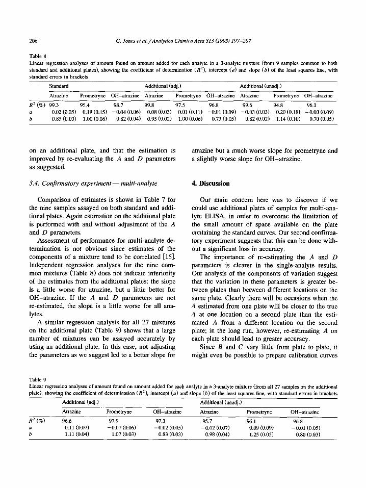
Table 8

Linear regression analyses of amount found on amount added for each analyte in a 3-analyte mixture (from 9 samples common to both

standard and additional plates), showing the coefficient of determination CR’), intercept (a) and slope (b) of the least squares line, with

standard errors in brackets

Standard

Atraxine

Additional (adj.) Additional (unadj.)

Prometryne OH-atrazine Atrazine Prometryne OH-atrazine Atrazine Prometryne OH-atrazine

R* (%) 99.3 95.4 98.7 99.8 97.5 96.8 99.6 94.8 96.1 a 0.02 (0.05) 0.19 (0.15) - 0.04 (0.06) 0.08 (0.03) 0.01 (0.11) - 0.01 (0.09) - 0.03 (0.03) 0.20 (0.18) - 0.00 (0.09)

b 0.85 (0.03) 1.00 (0.08) 0.82 (0.04) 0.95 (0.02) 1.00 (0.06) 0.73 (0.05) 0.82 (0.02) 1.14 (0.10) 0.70 (0.05)

on an additional plate, and that the estimation is improved by re-evaluating the A and D parameters as suggested.

3.4. Confirmatory experiment - multi-analyte

Comparison of estimates is shown in Table 7 for the nine samples assayed on both standard and additional plates. Again estimation on the additional plate is performed with and without adjustment of the A and D parameters.

Assessment of performance for multi-analyte determination is not obvious since estimates of the components of a mixture tend to be correlated [15]. Independent regression analyses for the nine common mixtures (Table 8) does not indicate inferiority of the estimates from the additional plates: the slope is a little worse for atrazine, but a little better for OH-atrazine. If the A and D parameters are not re-estimated, the slope is a little worse for all analytes.

A similar regression analysis for all 27 mixtures on the additional plate (Table 9) shows that a large number of mixtures can be assayed accurately by using an additional plate. In this case, not adjusting the parameters as we suggest led to a better slope for

atrazine but a much worse slope for prometryne and a slightly worse slope for OH-atrazine.

4. Discussion

Our main concern here was to discover if we could use additional plates of samples for multi-analyte ELISA, in order to overcome the limitation of the small amount of space available on the plate containing the standard curves. Our second confirmatory experiment suggests that this can be done without a significant loss in accuracy.

The importance of re-estimating the A and D parameters is clearer in the single-analyte results. Our analysis of the components of variation suggest that the variation in these parameters is greater between plates than between different locations on the same plate. Clearly there will be occasions when the A estimated from one plate will be closer to the true A at one location on a second plate than the estimated A from a different location on the second plate; in the long run, however, re-estimating A on each plate should lead to greater accuracy.

Since B and C vary little from plate to plate, it might even be possible to prepare calibration curves

Table 9 Linear regression analyses of amount found on amount added for each analyte in a 3-analyte mixture (from all 27 samples on the additional

plate), showing the coefficient of determination CR*), intercept (a) and slope (b) of the least squares line, with standard errors in brackets

Additional (adj.) Additional (unadj.)

Atrazine Prometryne OH-atrazine Atrazine Prometryne OH-atrazine

R2 (o/o) 96.6 97.9 97.3 95.7 96.1 96.8

0.11 (0.07) - 0.07 (0.06) - 0.02 (0.05) - 0.02 (0.07) 0.09 (0.09) - 0.01 (0.05)

1.11 (0.04) 1.07 (0.03) 0.83 (0.03) 0.98 (0.04) 1.25 (0.05) 0.80 (0.03)

G. Jones et al./Analytica Chimica Acta 313 (199.5) 197-207 207

just once per day per lab and to use these for subsequent assays. Alternatively Bayesian methods, in which plausible values for the parameters are

up-dated using observed data, could be used to get accurate estimates using fewer calibration points [28].

An important point of general concern in the use of microtiter plate-based immunoassay is the extent to which the relationship between the response and the analyte concentration varies from one location to

another on the same plate (see also [17]). Earlier generations of 96-well plates often showed high

variability of protein attachment when used in ELISA; this was especially true of the outer wells

usually on two of the four sides. The optical and adsorptive properties of plates have improved dra-

matically, although it is still advisable to check a shipment of plates for within-plate consistency. In

addition to the plates themselves there are experimental contributions to within-plate variation. There may be ways of reducing or accommodating this variation: some procedural, such as preventing a temperature gradient from developing across the

plates; some statistical, such as the judicious design of the plate template, or estimating and adjusting for spatial correlation. Such methods could lead to fur- ther improvement in what is already a sensitive and accurate technique.

Acknowledgements

Research supported by NIEHS Super-fund 2P42-

ES04699, NSF DMS 95-10511, US EPA CR 819047, USDA Forest Service NAPIAP R8-27, Center for Ecological Health Research CR 819658, NIEHS Center for Environmental Health Sciences IP30-

ES05707 and Water Resources Center grant No. W-840. B.D. Hammock is a Burroughs Wellcome

Toxicology Scholar. M. Wortberg is a fellow of the Deutsche Forschungsgemeinschaft.

References

[I] J.C. Hall, R.J.A. Deschamps and M.R. McDermott, Weed

Technol., 4 (1990) 226.

[2] B.D. Hammock, S.J. Gee, Y.K. Cheung, T. Miyamato, M.H.

Goodrow, J.M. Van Emon and J.N. Seiber, in R. Greenhalgh

and T.R. Roberts (Eds.), Pesticide Science and Biotechnol-

I31

[41

[Sl

[61

[71

[81

[91

[lOI

1111

I121 [131

[I41

[I51

I161

[I71

1181

[191

[201

l211

I221

1231

l241

I251

A.D. Lucas, H.K.M. Bekheit, M.H. Goodrow, A.D. Jones, S.

Kullman, F. Matsumura, J.E. Woodrow, J.E. Seiber and B.D.

Hammock, J. Agric. Food Chem., 41 (1993) 1523.

M.H. Goodrow, R.O. Harrison and B.D. Hammock. J. Agric.

Food Chem.. 38 (1990) 990.

P. Tijssen. in R.H. Burdon and P.H. van Knippenberg (Eds.),

Laboratory Techniques in Biochemistry and Molecular Biol-

ogy, Elsevier, Amsterdam, 1990.

D.S. Bunch, D.M. Gay and R.E. Welsch, ACM Transactions

on Mathematical Software, 19 (1993) 109-130.

M.A. O’C’onnell, B.A. Belanger and P.D. Haaland, Chemom.

Intell. Lab. Syst., 20 (1992) 97.

1261 S.R. Searle, Linear Models, Wiley, New York, 1971.

1271 SAS Institute Inc., SAS/STAT User’s Guide, version 6, 4th

edn., volume 2, SAS Institute Inc., Cary, NC.

[28] J.D. Unadkat, S.L. Beal and L.B. Sheiner, Anal. Chim. Acta, 181 (1986) 27.

ogy, Symposium Proceedings of the International Union of

Pure and Applied Chemistry, Blackwell. London, 1987, p.

309.

E. Ishikawa, S. Hashida, T. Kohno and K. Hirato, J. Clin.

Lab. Anal.. V7 N6 (1993) 376.

E. lshikawa and T. Kohno, 1. Clin. Lah. Anal., V3 N4 (198Y)

252.

F. Jung, S.J. Gee, R.Q. Harrison, M.H. Goodrow, A.E. Karu,

A.L. Braun, Q.X. Li. and B.D. Hammock, Pestic. Sci., 26

(1989) 303.

M. Vanderlaan, B.E. Watkins and L. Stanker, Environ. Sci.

Technol., 22 (1988) 247.

J.M. Van Emon, J.M. Seiber and B.D. Hammock, Anal.

Methods Pestic. Plant Growth Regul., 17 (1989) 217.

D. Rodbard, in S. Natelson, A.J. Pescc and A.A. Dietz

(Eds.), Clinical Immunochemistry, American Association for

Clinical Chemistry, Washington, DC, 1978. p. 477.

D.J. Finney, Statistical Methods in Biological Assay, 3rd

edn., Griffin, High Wycombe, 1978.

A. De Lean. P.J. Munson and D. Rodbard, Am. J. Phys.

Endocrinol. Metab. Gastrointest. Physiol.. 4 (1978) E97.

D. Rodbard, in J. Langan and J.J. Clapp (Eds.), Ligand

Assay: Analysis of International Developments on Isotopic

and Nonisotopic Immunoassay. Masson, New York, 1981.

D.J. Finney, Clin. Chem., 29 (1983) 1762.

G.M. Raab, Clin. Chem., 29 (1983) 1757.

G. Jones, M. Wortberg, S.B. Kreissig, D.S. Bunch, S.J. Gee,

B.D. Hammock and D.M. Rocke, J. Immunol. Methods, in

press.

M. Wortberg, S.B. Kreissig, G. Jones, D.M. Rocke and B.D.

Hammock, 304 (1995) 339..

S.B. Kreissig, M. Wortberg, G. Jones, D.M. Rocke, S.G.

Gee, P.V. Choudary and B.D. Hammock, in preparation.

I.C. Shekarchi, J.L. Sever, Y.J. Lee, G. Castellano and D.L.

Madden, J. Clin. Microbial., 19 (1984) 89.

A.E. Karu, R.O. Harrison, D.J. Schmidt. C.E. Clarkson, J.

Grassmann, M.H. Goodrow, A.D. Lucas, B.D. Hammock,

J.M. Van Emon and R.J. White, ACS Symp. Ser., 451 (1991)

59.

T. Giersch and B. Hock, Food Agric. Immunol., 2 (1990) 85.

R.O. Harrison, M.H. Goodrow and B.D. Hammock, J. Agric.

Food Chem., 39 (1991) 123.

Sources of experimental variation in calibration curves for enzyme-linked immunosorbent assay

Documents

Transcript of Sources of experimental variation in calibration curves for enzyme-linked immunosorbent assay