SãoPauloJournalofMathematicalSciences …spjm/articlepdf/505.pdf · associated to the Tent and...

São Paulo Journal of Mathematical Sciences 8, 2 (2014), 241–263

Copulas, Chaotic Processes and Time Series: aSurvey

Guilherme PumiMathematics Institute - Federal University of Rio Grande do SulE-mail address: [email protected]

Sílvia R.C. LopesMathematics Institute - Federal University of Rio Grande do SulE-mail address: [email protected]

Abstract. In this work we summarize some of recent and classical re-sults on the role played by copulas in the analysis of chaotic processesand univariate time series. We review some aspects of the copulasrelated to chaotic process, its properties and applications. We alsopresent a review on classical and modern approaches to understandthe relationship among random variables in Markov processes as wellas short and long memory time series as well as ergodic properties ofcopula-based Markov processes.

Keywords. Chaotic Processes, Copulas, Interval Maps, InvariantMeasures, Parametric Estimation.

1. IntroductionThis paper aims to present a brief survey on the study of copulas

and its relationship with chaotic process and univariate time series. Thiswork does not intend to be complete or in-depth, but rather to reflect thepreferences and the research conducted by the authors on these subjects.

For any set of random variables X1, · · · , Xn with joint distributionfunction H and marginals F1, · · · , Fn, respectively, copulas are a veryhelpful tool for understanding statistical properties of these family ofdistributions and, consequently, of the vector (X1, · · · , Xn)′.

The name “copula” dates back to the work of Sklar (1959), where thecelebrated Sklar’s theorem was first proven. The use of such functions,however, predates Sklar’s work. Sklar’s theorem is considered the most

241

242 G. Pumi and S. R. C. Lopes

important theorem in the theory because it elucidates the role playedby copulas on “coupling”, that is, tieing together any multivariate dis-tribution with its marginals. Sklar’s theorem is also the base of most,if not all, applications of copulas in statistics and stochastic processes.The reader interested on the history of copulas is referred to Schweizer(1991), Schweizer and Sklar (2005), Nelsen (2006) and references therein.

The interest on copulas in late 1950’s to early 1980’s was motivated bythe development of the theory of probabilistic metric spaces. Althoughmost of the crucial theorems on the theory of copulas dates back to thatepoch, the theory of copulas became dormant for almost a decade whenin late 1980’s to early 1990’s, the discovery of new applications of copulasin finances and statistics, renewed the interest on them. After late 1990’sthe theory and application of copulas and its ramifications to stochasticprocesses grew enormously. For an account of these developments seeNelsen (2006) and Cherubini et al. (2004). More details on copulas willbe provided in Section 2.

Consider a smooth function T : I → I, where I := [0, 1], and assumeµT is a T -invariant probability measure. Let U0 be a random variabledistributed as µT . We can define a stochastic process by setting

Xt := ϕ(T t(U0)

), t ∈ N, (1.1)

for a given µT -integrable function ϕ : [0, 1] → R. This is often calleda (pure) chaotic process. In the literature, however, sometimes a signalplus noise type of process where the signal is the process defined in (1.1)plus a random noise is considered. In this work we shall call a chaoticprocess such the one defined in (1.1).

From the definition of chaotic process, we observe that, for a givenfixed ω, Xt(ω) = ϕ

(T t(U0(ω))

)and, from setting w0 := U0(ω), we see

that the trajectory {Xt(ω)}t∈N is the avaliation of ϕ in the t-th iterationof T in the initial point w0. This means that a realization of {Xt}t∈Ncan be seen as a deterministically generated sequence. Nevertheless, arealization of such process present a complex/chaotic dynamics, withvery unstable and erratic behavior and instability with respect to theinitial point w0 = U0(ω). This type of process has been applied on avariety of problems from rock drilling to the study of intermittency onhuman cardiac rate (see Zebrowsky, 2001, Lasota and Mackey, 1994 andreferences therein). As an illustration, Figure 1 shows two sample pathsof the Manneville-Pomeau process for two initial points distant 0.0001of one another. Notice that after 10 steps or so the two sample pathsbecome far apart.

São Paulo J.Math.Sci. 8, 2 (2014), 241–263

Copulas, Chaotic Processes and Time Series: a Survey 243

Figure 1. Two realizations of the Manneville-Pomeau pro-cess for 2 distinct initial points distant 10−3 from each other.

Although the literature on dynamical system and ergodic theory relatedto these type of processes is vast (see Lasota and Mackey, 1994, Pollicottand Yuri, 1998 and references therein), the statistics aspects related tosuch processes is still in its infancy and has seen grown attention in the lastdecade (see, for instance, Chazottes et al., 2005 and references therein).Olbermann et al. (2007), Lopes and Pumi (2013) and Pumi and Lopes(2013a) discuss parameter estimation on chaotic process while parameterestimation on a signal plus noise setting is discussed in Lopes and Lopes(1998).

The connection between copulas and dynamical systems/ergodic theoryis also a subject not very much explored. Some works on this direction areKolesárová et al. (2008), Lopes and Pumi (2013), Pumi and Lopes (2013a)and Schmidl et al. (2013).

The interest in the connections between copulas and stochastic pro-cess/time series has also seem a grown of attention in the last years. Mostof the literature is based on the seminal paper on copula-based Markov pro-cesses by Darsow et al. (1992) and later development by Ibragimov (2009)on copula-based higher order Markov processes. See also Pumi and Lopes(2013b) and references therein.

Our paper is organized as follows: in the next section we consider somepreliminaries results necessary to the work. Section 3 presents some nomen-clature and review some facts on chaotic process while in Section 4 we dis-cuss the copulas related to certain chaotic processes, approximations andapplications in parameter estimation in these processes. In Section 5 wereview the literature on copula-based Markov process as well as considersome extensions to time series with non-Markovian dependence, includinglong-range dependent ones. In Section 6 we present an application andSection 7 concludes the paper.



2. Preliminaries

We start by recalling some facts on copulas. An n-dimensional copula isa distribution function for which the marginals are uniformly distributedon I and whose support is contained in the hypercube In. We recall thatthe support is the whole hypercube In only when the independence copulais considered. The usefulness of copulas in applications lies on its capabilityto allow the manipulation of the joint and marginal dependence structureseparately from each other, leading to great flexibility.

Copulas have been successfully applied and widely spread in several ar-eas. In finances, copulas have been applied, and become standard tools, inmajor topics such as asset pricing, risk management and credit risk analysisamong many others (see the books by Cherubini et al., 2004 and McNeilet al., 2005 for details). In hydrology, the modeling of rainfalls and stormsoften employ copulas to describe joint features among variables in the mod-els (see, for instance, Palynchuk and Guo, 2011 and references therein). Ineconometrics, copulas have been widely employed in constructing multidi-mensional extensions of complex models (see, for instance Lee and Long,2009, Wang et al., 2009 and references therein). In statistics, copulas havebeen applied in all sort of problems, such as development of dependencemeasures, modeling, testing, just to cite a few (see Mari and Kotz, 2001,Nelsen, 2006 and references therein). It has also been successfully appliedas a tool in simulation of time series and stochastic processes for which itis desired to compare different marginal structure under exactly the samejoint structure and vice-versa. See, for instance, Lopes et al. (2013).

The main result in the theory of copulas is the celebrated Sklar’s theorem,which we recall below. Sklar’s theorem unravel the role played by copulason coupling a multivariate distribution to its marginals and vice-versa. Theoriginal proof is due to Sklar (1959), but see Rüschendorf (2009) for aconsiderably simpler proof in the n-dimensional case and Nelsen (2006) fora more detailed proof in the bidimensional case on the lines of Sklar (1959).Theorem 2.1 (Sklar’s Theorem). Let X1, · · · , Xn be random variables withjoint distribution function H and marginals F1, · · · , Fn, respectively. Then,there exists a copula C such that

H(x1, · · · , xn) = C(F1(x1), · · · , Fn(xn)

), for all (x1, · · · , xn) ∈ Rn.

If the Fi’s are continuous, then C is unique. Otherwise, C is uniquelydetermined on Ran(F1)× · · · × Ran(Fn), where Ran(F ) denotes the rangeof the function F . The converse also holds. Furthermore,C(u1, · · · , un) = H

(F

(−1)1 (u1), · · · , F (−1)

n (un)), for all (u1, · · · , un) ∈ In,

where for a function F , F (−1) denotes its pseudo-inverse given by F (−1)(x):= inf

{u ∈ Ran(F ) : F (u) ≥ x

}.



For more details on the theory of copulas and its applications we referto the books by Joe (1997), Cherubini et a. (2004), McNeil et al. (2005)and Nelsen (2006).

3. Chaotic Processes

Before proceeding further we need to establish some notation and somenomenclature, on the lines of Pumi and Lopes (2013a). We consider piece-wise monotone maps with finitely many branches T : I → I for whicheach branch is of class C1+α, for α ∈ (0, 1) (the class of differentiable func-tions whose derivatives are α-Hölder continuous). Each branch is definedin Ik which is assumed to be of the form Ik := [ak−1, ak), k = 1, · · · , swhere {a0, · · · , as} are the discontinuity points of T . We assume T (Ik) =T ([ak−1, ak)) = [0, 1) is a bijection for each k = 1, · · · , s. Also, without lossof generality, T will be assumed to be right continuous, except at 1, whereit will be taken as left continuous. A map T satisfying these conditionsis called finitely piecewise monotone C1+α function. We shall denote theset of finitely piecewise monotone C1+α functions for which there exists anabsolutely continuous invariant probability measure µT by T .

Examples of piecewise monotone maps of such functions T are the fol-lowing:

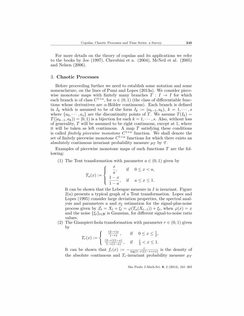
(1) The Tent transformation with parameter a ∈ (0, 1) given by

Ta(x) :=

x

a, if 0 ≤ x < a,

1− x1− a , if a ≤ x ≤ 1.

It can be shown that the Lebesgue measure in I is invariant. Figure2(a) presents a typical graph of a Tent transformation. Lopes andLopes (1995) consider large deviation properties, the spectral anal-ysis and parameters a and σξ estimation for the signal-plus-noiseprocess given by Zt = Xt + ξt = ϕ(Ta(Xt−1)) + ξt, when ϕ(x) = xand the noise {ξt}t∈N is Gaussian, for different signal-to-noise ratiovalues.

(2) The Giampieri-Isola transformation with parameter r ∈ (0, 1) givenby

Tr(x) :=

(2−r)x1−rx , if 0 ≤ x ≤ 1

2 ,

(2−r)(1−x)1−r(1−x) , if 1

2 < x ≤ 1.It can be shown that fr(x) := − r

log(1−r)(1−r+rx) is the density ofthe absolute continuous and Tr-invariant probability measure µT



(cf. Giampieri and Isola, 2005). Figure 2(b) presents a typicalgraph of a Giampieri-Isola transformation.

Recall that, the T -invariant probability measure considered here is ab-solutely continuous with respect to the Lebesgue measure on I. Underdifferent hypothesis one can show the existence of such kind of probabil-ity measure. The literature in the subject is vast, see for instance Réinyi(1957), Lasota and Yorke (1973), Bowen (1979), Pianigiani (1980, 1981),Inoue and Ishitani (1991) and references therein, just to cite a few.

We observe that if T has s ≥ 1 full branches, then T h will have sh fullbranches. For T ∈ T with s > 1 full branches, we shall denoteK↑t := {k : T t|Ik

is increasing} and K↓t := {k : T t|Ikis decreasing}.

(3.2)We formally define the class of chaotic process we are interested here.Definition 3.1. Let T ∈ T and let µT be the corresponding T -invariantprobability measure. Let U0 be a random variable distributed according toµT and ϕ : I → R be a function in L1(µT ). The stochastic process givenby

Xt := (ϕ ◦ T t)(U0), for all t ∈ N, (3.3)is called a Tϕ-induced process (or Tϕ process, for short).

Figures 2(d) and 2(e) present a typical realization of the Tϕ processassociated to the Tent and Giampieri-Isola transformation, respectively.Figure 2(c) presents the graph of the transformation given by

Ta,b(x) :=

a+ (1−a)xb , if 0 ≤ x < b,

a(x−b)1−b , if b ≤ x < 1,

(3.4)

where a, b ∈ (0, 1). It can be shown that there exists an absolutely contin-uous Ta,b-invariant probability measure (cf. Coelho et al., 1995), but sincethe transformation does not have full branches, it follows that Ta,b /∈ T .Figure 2(f) presents a typical realization of the process given by (3.3) asso-ciated to Ta,b(·), given by (3.4). Notice the contrast with the other cases.Lopes and Lopes (1998) consider large deviation properties, the spectralanalysis and parameters α, β and σξ estimation for the signal-plus-noiseprocess given by Zt = Xt + ξt = ϕ(T ta,b(X0)) + ξt, when ϕ(x) = x andthe noise is Gaussian, for different signal-to-noise ratio values. The valuesα and β are related to the values a and b of the Ta,b(·) transform by therelationship α = T ′a,b(x) = 1−a

b , if 0 ≤ x < b and β = T ′a,b(x) = a1−b , if

b ≤ x ≤ 1.Given T ∈ T , without further mention we shall consider that an ab-

solutely continuous T -invariant probability measure has been fixed which



(a) (b) (c)

(d) (e) (f)

Figure 2. Typical graph of the (a) Tent transformation;(b) Giampieri-Isola transformation and (c) transformation(3.4). Typical sample from (3.3) with T as (d) Tent transfor-mation with parameter a = 0.8; (e) Giampieri-Isola trans-formation with parameter r = 0.8; (f) transformation (3.4)with parameters a = 0.8 and b = 0.6. In all cases ϕ(x) = xand x0 =

√2(mod 1).

shall be denoted by µT , except otherwise explicitly said. Now let ϕ ∈L1(µT ) be an almost surely increasing function and consider {Xt}t∈N theTϕ process associated to T . For all t ∈ N, let Ft(·) be the distributionfunction of Xt. The T -invariance of µT , implies that, for any t ∈ N, t > 0,and x ∈ I,

Ft(x) := P(T t(U0) ≤ x

)= µT

((T t)−1([0, x]

))= µT

([0, x]

)= F0(x). (3.5)

Hence, a Tϕ process is always strongly stationary. Also, µT � λ impliesthat µT is non-atomic and therefore, Ft is continuous, increasing and itsinverse is well defined.



We need to further introduce a notation for the inverse image of a single-ton y ∈ I by a transformation T ∈ T . For T ∈ T with s > 1 full branches,the restriction of T h to each branch Ik defines a bijective map for which theinverse is well-defined. This inverse, denoted by Th,k(y) := (T h)−1|Ik

(y),can be then written as a vector

(T t)−1(y) =((T t)−1|I1(y), · · · , (T t)−1|Ist (y)

)=(Tt,1(y), · · · , Tt,st(y)

).

4. Copulas Related to Chaotic Processes

In this section we shall review some of the results in the literature oncopulas and chaotic process of the form (3.3). The main idea in this case isto study the copulas related to vectors coming from {Xt}t∈N. In Lopes andPumi (2013) the authors study the chaotic process induced by the so-calledManneville-Pomeau transformation (MP transformation, for short) givenby

Ts(x) = x+ x1+s(mod 1),for s > 0. When s ∈ (0, 1), there exists a Ts-invariant probability measureso that Ts ∈ T when s ∈ (0, 1). The induced chaotic process is called theManneville-Pomeau process (MP process for short) and the copulas relatedto any vector of an MP process are called Manneville-Pomeau copulas (MPcopulas for short). Figure 3 show the graph of the Manneville-Pomeautransformation and a typical sample path of the MP process. In Lopes andPumi (2013) the authors derive the MP copulas in the bidimensional andmultidimensional cases, when ϕ is a monotone function. These copulasare shown to be singular with respect to the two-dimensional Lebesguemeasure and their support, on the bidimensional case, is shown to be thelines connecting the discontinuity points of the MP transformation. Weshall refrain from presenting the explicit formulas for the MP copulas here,as they are a particular case of what will be presented in the subsequent.

Lopes and Pumi (2013) also consider some computational issues, ap-proximations and random variate generation problems related to the MPprocesses. In this work the authors also derive a fast procedure to estimatethe underlying parameter in Manneville-Pomeau processes. In Pumi andLopes (2013a), the authors derive the copulas related to any transforma-tion T ∈ T . Let T ∈ T , µT be the T -invariant probability measure and{Xt}t∈N be the associated Tϕ process for ϕ ∈ L1(µT ) an almost everywhereincreasing function. For simplicity, let Fh,k : I → [F0(ah,k−1), F0(ah,k)] bethe functions defined by

Fh,k(x) := F0

(Th,k

(F−1

0 (x))), (4.6)

for h > 0 and k ∈ {1, · · · , sh}. For a given set S, we also define δS(u)as being 1, if u ∈ S, and 0, otherwise. If we let {ah,k}s

h

k=0 denote the



(a) (b)

Figure 3. (a) Graph of the Manneville-Pomeau transfor-mation for s ∈ {0.1, 0.5, 0.9}; (b) a typical sample path ofan MP process.

discontinuity points of T h, then the copula related to (Xt, Xt+h) is givenbyCXt,Xt+h

(u, v) =∑

k∈n↑0

[Fh,k(v)− F0(ah,k−1)

]+

+[

min{u,Fh,n0(v)

}− F0(ah,n0−1)

]δ

K↑h

(n0) +

+∑

k∈n↓0

[F0(ah,k)−Fh,k(v)

]+ max

{0, u−Fh,n0(v)

}δ

K↓h

(n0),

(4.7)

where n0 := n0(u;h) ={k : u ∈

[F0(ah,k−1), F0(ah,k)

)}, and, with K↑h and

K↓h as in (3.2),

n↑0 :=

{1, · · · , n0 − 1}⋂K↑h, if n0 > 1;

∅, if n0 = 1;and

n↓0 :=

{1, · · · , n0 − 1}⋂K↓h, if n0 > 1;

∅, if n0 = 1.We notice that if T is taken to be the MP transformation for s ∈ (0, 1),then n↓0 = ∅ and we obtain the MP copula of (Xt, Xt+h) upon the obvioussubstitution on (4.7) (Lopes and Pumi, 2013 applies a slightly differentindexing for the sets involved). In Pumi and Lopes (2013a) it is shownthat the copulas related to any bidimensional vector (Xt, Xt+h) from a Tϕ



process is singular with respect to the Lebesgue measure and its supportcomprehend the graph of the lines joining the consecutive discontinuitypoints of T h. In Figure 4 we show the three dimensional plots of the lag2 MP copula, the level plots and 500 sample points obtained with theapproximations presented.

Figure 4. From left to right, upper panel, three dimen-sional plots of the lag 2 MP copula for s ∈ {0.1, 0.4} andrespective level sets obtained using approximations. On thebottom panel, 500 approximated sample points from a lag2 MP copula for s ∈ {0.1, 0.4}

The copulas related to n-dimensional vectors from a Tϕ process can alsobe shown to be singular with respect to the Lebesgue measure, but itssupport is much harder to describe. In the multivariate case, the formulaof the copulas related to Tϕ processes are involved and we shall refrainfrom showing them here, but they are explicitly derived in Pumi and Lopes(2013a) (and so is the multivariate MP copula in Lopes and Pumi, 2013).

4.1. The Need of Approximations. For concrete applications it is nec-essary to have a closed form for the copula. In order to calculate copulasof random variables coming from chaotic processes related to a T map oneneeds an explicit form for the density of the T -invariant probability measureµT . In practice, however, finding a closed form of such probability mea-sure is usually a non-trivial task. In most cases when such a probabilitymeasure exists, it does not have a closed formula. But since the copulas de-pend on µT through F0 and F−1

0 , non-explicit formula for µT translates asnon-explicit formulas for the copulas. Another potentially complex task isdetermining precisely the discontinuity points of a map T , and if the exact



location of such points cannot be analytically determined, it means that thecopula cannot be explicitly determined either. So in practice there is a needto develop approximations for these (and other) elements to implement andanalyze the studied copulas.

More explicitly, the elements to be known in other to determine thecopulas related to bidimensional vectors coming from a Tϕ process are thedistribution function F0 and its inverse F−1

0 , the inverse of T h in eachbranch ({Th,k}s

h

k=1) and the discontinuity points {ah,k}sh

k=0 associated to T h.In the case where T ∈ T , an approximation to the T invariant measure µTbased on a sample of size n of the respective Tϕ process, say x0, · · · , xn−1,at a µT -continuity set A is

µn(A;T, x0) := 1n

n−1∑k=0

δxi(A).

An approximation F̂n to the distribution F0 is then obtained through theobvious relationship F̂n(x) := µn

([0, x];T, x0

). Notice that in this context,

F̂n is just the empirical distribution calculated on the data, so that theapproximation F̂−1

n for F−10 can be taken as the empirical quantile function,

or an interpolation method can be used to improve the local estimation ofF̂−1n based on the empirical quantile function.In the case where T is the Manneville-Pomeau transformations, Lopes

and Pumi (2013) present some empirical results on the convergence of theseapproximations, which were found to be satisfactory and well-behaved withrespect to x0 even though, as mentioned before, the process itself is not.The authors apply a linear interpolation over the values of the empiricalquantile function as approximation to F−1

0 .There is no general optimal way to approximate neither the inverse image

of T h nor its discontinuity points. In Lopes and Pumi (2013) a methodbased on the empirical inverse of T h and a linear interpolation step isused for the case of the Manneville-Pomeau transformation. A generaland relatively precise way to approximate {Th,k}s

h

k=1 and {ah,k}sh

k=0 in thecase T ∈ T is devised in Pumi and Lopes (2013a). The method is based onisolating the points on each branch. On each given branch, an interpolationon the point nearest to the end points of the branch and the closest one onthe adjacent branch±1, depending whether the transformation is increasingor decreasing on the branch, is performed. However, the authors presentexamples where simpler and faster ways to determine the inverse image anddiscontinuity points of a transformation exist in some specific cases.



The approximations devised in both papers are shown to be uniformlyconvergent to their targets. The approximation to the copula is then ob-tained by plugging-in these intermediate approximations directly into theformula of the copula. Lopes and Pumi (2013) show that the approximationto the copula, in the bidimensional case, converges to the true MP copulaas the sample size increases and the result holds uniformly in I2. Pumiand Lopes (2013a) show more: in the bidimensional case, as long as theintermediate approximations applied converge uniformly to their targets,the approximation to the copula will converge uniformly in I2 to the truecopula. These results are exemplified through Monte Carlo experiments inboth, Lopes and Pumi (2013) in the context of MP copulas and in Pumiand Lopes (2013a) in the more general case of Tϕ processes.

The problem of random variate generation in the bidimensional case isalso discussed in Lopes and Pumi (2013) and Pumi and Lopes (2013a).Given that the support of the copula of (Xt, Xt+h) is simply the line con-necting adjacent discontinuity points of T h, the following general simplemethod can be used: take u a random variate from an U(0, 1) distribution.This point will lie on a certain branch of T h, say the k-th branch. Set v asthe image of u by the linear function connecting the endpoints in the k-thbranch. The desired point is then (u, v).

4.2. Application to the Parameter Estimation in Chaotic Pro-cesses. Parametric estimation on a signal-plus-noise context was first con-sidered in Lopes and Lopes (1998). Through examples that generalize theclassical harmonic model, the authors present a method for obtaining thespectral distribution functions and large deviation properties of the esti-mated parameters of the model. Parametric estimation on Manneville-Pomeau processes was considered in Olbermann et al. (2007). The idea inthe paper is to apply classical spectral density based estimators from thetheory of long-range dependent time series in order to estimate the param-eter of the Mannevile-Pomeau transformation. This idea was motivated bythe fact that, on certain regions, the MP process presents slow decay ofcorrelation (see, for details, Olbermann et al., 2007 and references therein).

In Lopes and Pumi (2013) a method for parameter estimation on MPprocesses inspired by the theory developed is devised. The idea is to takeadvantage of the simple form of the support of the MP copula to makeinference on the parameter of the transformation. More specifically, givena sample x0, · · · , xn−1 from the MP process, the idea is to form a newsequence vi := (xi, xi+1), sort these vectors with respect to the branch theybelong to and them locally interpolate near the discontinuity points. Thiscan be achieved in several ways, see Lopes and Pumi (2013) for a leastsquare and a minimum-maximum type of interpolation as well as a MonteCarlo simulation study.



In Pumi and Lopes (2013a), three methods of estimation are discussed,but two of them (curiously, the more natural and straightforward ones) are,as the authors argue, computationally too expensive for practical applica-tions. The third method can be explained as follows. Let Tθ ∈ T , withs > 1 branches and θ := (θ1, · · · , θp) ∈ S ⊆ Rp, for 1 ≤ p ≤ s − 1. Let{ak}sk=0 denote the discontinuity points of Tθ. Suppose that θ is identifiablethrough the knowledge of the {ak}sk=0 alone, that is, θ := f(a0, · · · , as),where f : Is+1 → S is a known invertible function. Let {Xt}t∈N be the as-sociated Tϕ process and assume that ϕ is the identity map to fix the ideas.Let x1, · · · , xN be a sample from Xt. Since Tθ ∈ T , F0 is generally smoothso that, near each of its discontinuity points Tθ should behave close to alinear function. The procedure then is to identify the points that are closerto endpoints on a given branch and perform a linear interpolation betweenthese points and their respective images by Tθ (only one of then suffices).

This is a refinement of the minimum-maximum method in Lopes andPumi (2013). The authors present a Monte Carlo simulation study on thefinite sample performance of the estimator on certain chaotic process. Thesimulation results suggest that the procedure performs very well with smallbias and small variability. Also indicates that nuisance parameters do notaffect the parameter estimation.

5. Copulas and Univariate Time Series

In this section we present a brief survey about copula-based univariatetime series. This survey does not intend to be neither a thorough nor anin-depth work, but instead, it intends to reflect the author’s preferencesand their research on the subject.

Copulas are fundamentally a multivariate tool for understanding andmodeling joint dependence structure and marginal structure separately. Let{Xt}∞t=0 be a weakly stationary process.

From a strictly probabilistic/measure theoretical point of view, associ-ated to any time series, there is a sequence of distributions {Fn}∞n=0, andto every random vector (Xt1 , · · · , Xtn) from the process, there is an n di-mensional copula Ct1,··· ,tn associated to it. Describing how these copulasbehave starting from an univariate time series and how one can constructa time series starting from its copulas is the subject of many studies.

5.1. Markovian Framework. The seminal work of Darsow et al. (1992)provides a complete description of Markov processes in terms of copulas.More specifically, they studied how to translate the Chapman-Kolmogorovequations for transition probabilities into copulas framework. They alsostudy how to specify copulas for each pair (Xr, Xs) so that the resulting



process is a Markov process. This technique to construct copula-basedMarkov process is quite different from the usual ones in that one specifiescopulas and then the marginal distributions can be chosen at will. Givenits importance, we outline the methodology.

Fundamentally, the idea in Darsow et al. (1992) is to determine a certainproduct on the space of all bidimensional copulas and then to connect thisoperation to the theory of Markov processes. For any pair of bidimensionalcopulas C1 and C2, it is defined a product ∗ on the space of all copulas bysetting

(C1 ∗ C2)(u, v) :=∫I

∂C1(u, t)∂t

∂C2(t, v)∂t

dt.

In Darsow et al. (1992), several properties of the ∗ operation are dis-cussed. For instance, for two copulas C1, C2, C1 ∗ C2 is also a copula; asa binary operation in the space of copulas, ∗ is right and left distributiveover linear combinations, continuous in each place (but not jointly contin-uous), associative and the copulas M and Π are the identity and null ele-ments, respectively, with respect to ∗. All these properties together makethe set of all copulas with the operation ∗ and the transpose operation,CT (u, v) = C(v, u), a symmetric Markov algebra1.

If {Xt}t∈T , T ⊂ R, is a continuous time process for which we denote thecopula related to (Xs, Xt) by Cs,t. A necessary and sufficient conditionson the copulas in order to assure that {Xt}t∈T is a Markov process isgiven in Darsow et al. (1992). In particular they show that the transitionprobabilities of {Xt}t∈T satisfy the Chapman-Kolmogorov equations if andonly if Cs,t = Cs,u∗Cu,t for all s, t, u ∈ T , s < u < t. To specify a first orderMarkov chain in the simplest case where the marginal distributions do notvary over time (say F ), based on a single bidimensional copula C withdensity c, one observe that, from Sklar’s theorem, the conditional densityof Xt given Xt−1 (say fXt|Xt−1) can be written as

fXt|Xt−1(xt|xt−1) = c(F (xt−1), F (xt)

)f(xt−1).

More details can be found in Darsow et al. (1992) and in Section 6.4 ofNelsen (2006) and references therein. See also Lågeras (2010) which reportssome non-standard behavior of copula-based Markov chains.

Joe (1997) discusses how to construct short memory time series based onconditional copulas as well as a method of constructing short memory pro-cesses based on the parameterization of the distributions on a convolution

1In Darsow et al. (1992), a Markov algebra is defined as a compact convex subsetof a real Banach space on which a product is defined which is continuous in each place,associative, distributive over convex combinations and which possesses a null and unitelements. It is said to be symmetric if it possesses a continuous operation T such thatT(T (A)

)= A, T (AB) = T (B)T (A) and it is distributive under convex combinations.



closed family. Based on the well established theory of copula-based Markovprocesses constructed in Darsow et al. (1992), many works studied how tocharacterize short memory time series based on copulas, as well as how toapply these techniques on parameter estimation. One of the first rigorousapproach to this type of problem is given in Chen and Fan (2006) andlater augmented in Chen et al. (2009). These works study the problem ofsemiparametric estimation in a copula-based univariate strictly stationaryMarkov processes context.

The main idea is to notice that if one apply the integral probabilitytransform to a Markov process, the resulting process will still be a Markovprocess and the joint distributions are copulas. After that one can rewritethe original Markov process into a semiparametric generalized linear modeldepending on the copula and its parameter alone. Let {Xt}nt=1 be a samplefrom a stationary first order Markov process and let F be the true invariantdistribution. Suppose that F is absolutely continuous with respect to theLebesgue measure in R. Let Cθ be the true parametric copula associatedto the pair (Xt−1, Xt) up to an unknown parameter θ and suppose thatit is absolutely continuous with respect to the Lebesgue measure in I2.Also suppose that Cθ is neither of Fréchet-Hoeffding’s bounds. In thissetting, if one considers a new time series by setting Ut = F (Xt), t =1, · · · , n, the transformed process is still a stationary Markov process, thejoint distribution of (Ut−1, Ut) will be Cθ(u, v) and the conditional densityof Ut|Ut−1 = u0 will be fUt|Ut−1(u|u0) := cθ(u0, u). This implies that thissetting is consistent with the following semiparametric generalized linearmodel

ϕ(Ut) = ψ(Ut−1) + εt, E(εt|Yt−1) = 0,where ϕ is an increasing parametric function, ψ(·) is given by

ψ(u) = E(ϕ(Ut)

∣∣Ut−1 = u)

=∫ 1

0ϕ(v)cθ(u, v)du

and the conditional density of εt given Ut−1 = u0 is given by

fεt|Ut−1(x|u0) =cθ(u0, ϕ

−1(x+ ψ(u0)))

ddx

(ϕ(x+ ψ(u0)

)) .

To estimate the copula parameter, Chen and Fan (2006) apply a MLEmethod based on the rescaled empirical distribution while Chen et al.(2009) apply a sieve MLEmethodology. The authors argue that the method-ology is useful in certain financial and economic applications. A methodfor simulating such time series can be found in Pumi and Lopes (2010).

The study on copula-based Markov processes also includes some ergodictheoretical properties. Chen and Fan (2006) find sufficient conditions for



their copula-based Markov process to be β-mixing at (least) a polynomialrate. Beare (2010) derive a condition under which a copula-based Markovprocess presents geometric β-mixing. This condition translates into thecopula being absolutely continuous with square integrable density, a ratherstrong requirement that rules out, for instance, any copula presenting taildependence or asymmetry. Beare (2012) derive sufficient conditions on thegenerator of an Archimedean copula so that the related Markov processespresent geometric ergodicity. Chen et al. (2009) show the geometric ergod-icity of copula-based Markov processes obtained from some popular copulafamilies presenting tail dependence. Beare and Seo (2012) discuss in de-tail the property of time reversibility in copula-based Markov processes (inthis case the copula family must be exchangeable) and introduce a test fortime reversibility similar to the test of exchangeability for copulas in Nelsen(2007).

Recently the literature turned its focus to the study of higher order typesof dependence. Ibragimov (2009) extends the work of Darsow et al. (1992)to higher order Markov process. In particular, as intuitively expected,it is shown that a Markov process of order n is fully determined by itsn + 1-dimensional copula and its marginal distributions. Ibragimov andLentzas (2009) discuss the slow decay of some copula-based dependencemeasure which motivated the authors to define a non-standard definitionof “long-range dependence”. They present empirical evidences that, for theMarkov process based on the Clayton copula, the non-standard copula-based long-range dependence concept introduced points to the existenceof “long memory” on the simulated time series. However, the theoreticalresults in Chen et al. (2009) show that the Markov process based on theClayton copula actually presents short memory in the classical sense. Thisimplies that the copula-based long-memory concepts introduced in Ibragi-mov and Lentzas (2009) are not compatible with the classical definition oflong-range dependence.

5.2. Non-Markovian Framework. So far the works mentioned here onlyconsider Markovian processes. The main reason for that is that outside thewell-structured and well-developed theory of copula-based Markov process,it is hard to overcome the difficulties imposed by the so-called compatibilityproblem. In few words, the compatibility problem is an statement of thefact that given an arbitrary collection of

(n2)2-dimensional copulas, there

may not exist an n-dimensional copula whose bidimensional marginals arethe given copulas. This is probably the most important open problem inthe theory of copula to date.

Pumi and Lopes (2013b) present an alternative approach to deal withthe covariance decay based in copulas without relying on Markovian as-sumptions. For a process {Xt}∞t=0 with absolutely continuous marginal



distributions {Ft}∞t=0 and for a given parametric family of copulas {Cθ}θ∈Θsatisfying some minor regularity conditions, the authors investigate howto translate the covariance decay in the process into a parameterization{θn}∞n=1 for the respective copula family. The only joint assumption isthat the copulas related to a pair (Xr, Xs) belong to a predefined paramet-ric family, allowing the theory to cover (weakly and strongly) stationaryprocesses as well as non-stationary ones. This condition can be actuallyrelaxed to require that the pair (Xr, Xs) has a copula Cθr,s belonging to apredefined family for values of r and s such that |r − s| is large.

The main focus of Pumi and Lopes (2013b) is classical long-range de-pendent process, but the theory is developed in order to accommodate anytype of covariance decay, including convergence to a constant, which coversthe case when the variables Xt and Xt+h are asymptotically correlated.

The main advantage of the approach developed in Pumi and Lopes(2013b) is to be free from the compatibility problem. This is attainedby focusing on pairs (Xr, Xs) associating a copula Cθr,s and then studyingthe behavior of the covariance of the pair (Xr, Xs) as |r− s| increases. Thenon-standard results of Tiit (2002) on the compatibility problem providesthe necessary theoretical result to show the compatibility-free nature ofthis approach. The copula version of Hoeffding’s lemma, which connectsthe covariance between two random variables to its bidimensional copulaand marginal distribution, is also an important ingredient on the theory.

The conditions imposed on the particular chosen parametric family ofcopulas, say {Cθ}θ∈Θ, are the existence of a point {a ∈ Θ} such thatlimθ→aCθ(u, v) = Π(u, v) = uv, the independence copula, and, as a func-tion of its parameter, the copulas are twice differentiable in a neighborhoodof a. As shown in Pumi and Lopes (2013b), many widely applied familiesof copulas satisfy such requirements. Under these assumptions the authorsshow that, asymptotically, the covariance decay of (Xt, Xt+n) with copulaCθn behaves like the product of a certain function K(n) (depending onthe marginal distributions alone) and the behavior of the difference θn− a,as n increases. When the marginals of the process do not vary, K(n) isa constant and, hence, the behavior of θn − a dictates the long run co-variance behavior of the process. In the case where the copula family ismultiparametric, a similar result holds, with the decay being dominated bythe slowest decay among the parameter coordinates.

In Pumi and Lopes (2013b) a method for parameter estimation based onthe studied theory is proposed. The method is a multi-stage procedure. Let{Xt}t∈N be a process for which Xt is identically distributed with commonabsolutely continuous distribution F , for all t ∈ N and let {xt}nt=1 be asample from it. Assume that the bidimensional copulas related to theprocess belong to a predetermined parametric family {Cθ}θ∈Θ satisfying the



assumptions of the previous paragraph. We also assume that the covarianceof {Xt}t∈N at lag h is a known function R(h, γ) where γ is a parameter ofinterest identifiable from R(·). The first step in the procedure is to estimatethe marginal distribution based on the given sample, say F̂ , and then forma new time series yi := F̂ (xi), i = 1, · · · , n. From this new time serieswe construct a bidimensional process {u(s)

k }n−sk=1 by u

(s)i := (yi, yi+s), i =

1, · · · , n−s, where s ∈ N is a user-defined number called the starting lag ofestimation. Next an estimate of the copula parameter related to {u(s)

k }n−sk=1

is obtained, say θ̂s. In view of the developed theory, the quantity θ̂s − a isregarded as an estimate of the covariance decay at lag s. The procedure isrepeated until a sequence of estimates θ̂s, · · · θ̂s+m is obtained, where m > sis the maximum desired lag of estimation. Finally the estimated value ofγ is set to be the value that minimizes the distance between the observeddecay and the expected R(h, γ) one through some predetermined metric.

The authors discuss large sample properties of the proposed estimatorand prove its consistency under mild conditions. The authors also present aMonte Carlo study to determine the small sample properties of the proposedestimator. Simulation of stationary and non-stationary time series in thisframework is also discussed and an application to real data is presented. Inthe next section we show an application of the method to the S&P500.

6. Application

To exemplify the ideas presented on Section 5.2, we reproduce here theexample given in Pumi and Lopes (2013b). The methodology is appliedto the daily returns of the S&P500 US stock market index in the periodfrom January 01, 2000 to November 03, 2011 yielding a total sample sizeof n = 2, 980. Figure 5(a) to Figure 5(c) present the S&P500 time se-ries, the correspondent returns {rt}2979

t=1 and the absolute returns {|rt|}2979t=1 ,

respectively.It is commonly found that in financial time series related to stock market

indexes, the daily returns are uncorrelated while the absolute and squaredreturns present slow decay of covariance, usually proportional to n−β forβ ∈ [0.2, 0.4] (see Cont, 2001 and references therein and also Lopes andPrass, 2013 for the intradaily case). Our goal is to apply the methodologyin Pumi and Lopes (2013b) to estimate β. The study of the absolute andsquared returns in financial time series are of great importance since theycontain information about the (unobservable) volatility.

In order to do that we shall assume that the underlying process is stronglystationary and ergodic and that all underlying bivariate copulas belong to



(a) (b) (c)

Figure 5. S&P500 (a) original time series; (b) return timeseries; (c) absolute return time series.

the same one parameter copula family. The autocorrelation and the peri-odogram functions of the absolute return time series of the S&P500 indexis presented in Figure 6(a). The slow decay of the sample autocorrelationfunction and the pronounced peak at the zero frequency in the periodogramfunction are commonly found in this type of data and both suggest long-range dependence on the absolute return time series. Given the behaviorof the sample autocovariance function, it is often assumed that {|rt|}∞t=0follows an ARFIMA(p, d, q) model, so that estimation of d is of interest.

(a) (b) (c)

Figure 6. (a) Autocorrelation function; (b) periodogramfunction; (c) histogram of the S&P500 absolute return timeseries and the fitted exponential density.

The first step on the methodology is to estimate the underlying marginaldistribution of the data. As argue in Pumi and Lopes (2013b), an exponen-tial distribution seems to be a good fit for the data and, by using a MLEmethod, an Exp(10.688) distribution was found to be a good fit for thedata. Hence, we take F̂ ∼ Exp(10.688) as the estimator for the underlyingmarginals and set yi = F̂ (|rt|), t = 1, · · · , 2979.



Next step is to identify the underlying family of bidimensional copulasrelated to the process. Even though in the literature, the use of the Gauss-ian copula on financial data sets is often contested, the authors argue thatin this case it is perfectly reasonable to assume the bidimensional copulasto be Gaussian ones.

For the Gaussian copula with Exp(10.688) marginals, it can be showthat K1 ∼= 260.47 and K2 ∼= 40.53. The next step is to estimate the copulaparameter ρ from the pseudo samples {(yi, yi+s)}2979−s

i=1 . Figure 7 presentsthe estimated copula parameter obtained via maximum likelihood methodup to lag 400. Chosen a particular lag `, let ρ̂1, · · · , ρ̂` denote the estimatesobtained in the previous step. In Lopes and Pumi (2013b), three possibleestimators, based on different functions R(·, ·) are compared. For simplicitywe shall present one of the estimators. In this case we are assuming that theunderlying process is an ARFIMA(0, d, 0) process with exponentially dis-tributed marginals. In the literature, the correlation decay on the squaredreturns is observed to be proportional to n−β for β ∈ [0.2, 0.4] (see Cont,2001) and the relationship to the parameter d of an ARFIMA(0, d, 0) modelis β = 1− 2d. The estimator is defined through the following optimizationprocedure:

d̂ := argmind∈(−0.5,0.5)

{ 1m+ 1

s+m∑h=s

∣∣ρ̂h − Γ(d)−1h2d−1∣∣}, β̂ := 1− 2d̂.

For the data, d̂ = 0.3370 with 95% confidence interval (0.3320, 0.3432)which gives β̂ = 0.3260 with 95% confidence interval (0.3136, 0.3360), allcoherent with the findings reported on literature (see Cont, 2001 and refer-ences therein). These findings are also consistent with non-linear modelingof the S&P500 data as reported, for instance, in Prass and Lopes (2013)(see also references therein).

Figure 7. Copula parameter estimated values.



7. Conclusions

In this work we present a brief summary on the modern and classicalresults on the role played by copulas in the theory of chaotic processes andunivariate time series.

In Section 1 and 2 the problem is introduced and some results on copulasare briefly reviewed. In Section 3 we briefly review some facts on the the-ory of chaotic processes necessary to the work. We formally define chaoticprocesses, discuss some of its properties and introduce the class of trans-formations considered in the reviewed literature. We proceed in Section 4to review the connection between copulas and chaotic process and some ofits properties.

The copulas related to the class of chaotic processes considered hereusually do not present closed formulas so that the study and applicationof such copulas rely on approximations. Some ideas on the approximationspresented in the literature as well as applications to parameter estimationin chaotic process and random variate generation are also discussed.

In Section 5 we briefly review the connections between copulas and uni-variate time series through the copula lens. The section is divided in Mar-kovian and non-Markovian theory. In the Markovian case, we review someof the ideas in the seminal paper by Darsow et al. (1992) on the theory ofcopula-based Markov processes as well as some applications to the parame-ter estimation in copula-based (short memory) time series. We also brieflyreview some results on the ergodic properties of copula-based Markov pro-cesses. Some extensions are also discussed.

In the non-Markovian case we shortly discuss the compatibility-free ap-proach to general dependence in Pumi and Lopes (2013b), focusing on theideas behind the theory developed there and its applications. We also pro-vide an application of the methodology to real time series.

Acknowledgements. S.R.C. Lopes research was partially supported by CNPq-Brazil, byCAPES-Brazil, by Pronex Probabilidade e Processos Estocásticos - E-26/170.008/2008-APQ1 and also by INCT em Matemática.

References[1] Bowen, R. (1979). “Invariant Measures for Markov Maps of the Interval”. Com-

munications in Mathematical Physics, 69, 1-14.[2] Beare, B.K. (2010). “Copulas and temporal dependence”. Econometrica, 78(1),

395-410.[3] Beare, B.K. (2012). “Archimedean copulas and temporal dependence”. Econo-

metric Theory, 28(6), 1165-1185.[4] Beare, B.K. and Seo, J. (2012). “Time Irreversible Copula-Based Markov Models”.

University of California at San Diego, Economics Working Paper Series.



[5] Chazottes, J.-R., Collet, P. and Schmitt, B. (2005). “Statistical Consequences ofthe Devroye Inequality for Processes. Applications to a Class of Non-UniformlyHyperbolic Dynamical Systems”. Nonlinearity, 18(5), 2341-2364.

[6] Chen, X. and Fan, Y. (2006). “Estimation of Copula-Based Semiparametric TimeSeries Models”. Journal of Econometrics, 130, 307-335.

[7] Chen, X., Wu, W.B. and Yi, Y. (2009). “Efficient Estimation of Copula-BasedSemiparametric Markov Models”. Annals of Statistics, 37, 4214-4253.

[8] Cherubini, U., Luciano, E. and Vecchiato, W. (2004). Copula Methods in Finance.Chichester: Wiley.

[9] Coelho, Z., Lopes, A.O. and da Rocha, L.F. (1995). “Absolutely ContinuousInvariant Measures for a Class of Affine Interval Exchange Maps”. Proceedingsof the American Mathematical Society, 123(11), 3533-3542.

[10] Darsow, W.F., Nguyen, B. and Olsen, E.T. (1992). “Copulas and Markov pro-cesses”. Illinois Journal of Mathematics, 36(4), 600-642.

[11] Giampieri, M. and Isola, S. (2005). “A One-Parameter Family of Analytic MarkovMaps with an Intermittency Transition”. Discrete and Continuous DynamicalSystems, 12(1), 115-136.

[12] Ibragimov, R. (2009). “Copula-based characterizations for higher order Markovprocesses”. Econometric Theory, 25, 819-846.

[13] Ibragimov, R. and Lentzas, G. (2009). “Copulas and long memory”. HarvardInstitute of Economic Research. Discussion Paper No. 2160.

[14] Inoue, T. and Ishitani, H. (1991). “Asymptotic Periodicity of Densities and Er-godic Properties for Nonsingular Systems”. Hiroshima Mathematical Journal,21(3), 597 - 620.

[15] Joe, H. (1997). Multivariate Models and Dependence Concepts. New York: Chap-man & Hall.

[16] Kolesárová, A., Mesiar, R. and Sempi, C. (2008). “Measure-preserving Trans-formations, Copulæ and Compatibility”. Mediterranean Journal of Mathematics,5(3), 325-339.

[17] Lagerås, A.N (2010). “Copulas for Markovian Dependence”. Bernoulli, 16(2),331-342.

[18] Lasota, A. and Mackey, M.C. (1994). Chaos, Fractals, and Noise. StochasticAspects of Dynamics. New York: Springer-Verlag. 2nd. Edition.

[19] Lasota, A. and Yorke, J.A. (1973). “On the Existence of Invariant Measures forPiecewise Monotonic Transformations”. Transactions of the American Mathemat-ical Society, 186, 481-488.

[20] Lee, T-H. and Long, X. (2009). “Copula-based multivariate GARCH model withuncorrelated dependent errors”. Journal of Econometrics, 150(2), 207-218.

[21] Lopes, A. and Lopes, S.R.C. (1998). “Parametric Estimation and Spectral Anal-ysis of Piecewise Linear Maps of the Interval”. Advances in Applied Probability,30, 757-776.

[22] Lopes, S.R.C. and Prass, T.S. (2013). “Seasonal FIEGARCH Processes”. Com-putational Statistics and Data Analysis, 68, 262-295.

[23] Lopes, S.R.C. and Pumi, G. (2013). “Copulas Related to Manneville-PomeauProcesses”. Brazilian Journal of Probability and Statistics. 27(3), 322-356.

[24] Lopes, S.R.C., Pumi, G. and Zaniol, K. (2011). “Mallows distance inVARFIMA(0,d, 0) processes”. Communications in Statististics: Simulation andCompututation, 42(1), 24-51.

[25] Mari, D.D. and Kotz, S. (2001). Correlation and Dependence. London: ImperialCollege Press.



[26] McNeil, A.J., Frey, R. and Embrechts, P. (2005). Quantitative Risk Management:Concepts, Techniques and Tools. Princeton: Princeton University.

[27] Nelsen, R.B. (2006). An Introduction to Copulas. New York: Springer-Verlag.2nd. Edition.

[28] Nelsen, R.B. (2007). “Extremes of nonexchangeability”. Statistical Papers, 48,329-336.

[29] Olbermann, B.P, Lopes, S.R.C and Lopes, A.O. (2007). “Parameter Esti-mation in Manneville-Pomeau Processes”. Unpublished manuscript. Source:arXiv:0707.1600.

[30] Palynchuk, B.A. and Guo, Y. (2011). “A probabilistic description of rain stormsincorporating peak intensities”. Journal of Hydrology, 409(1-2), 71-80.

[31] Pianigiani, G. (1980). “First Return Map and Invariant Measures”. Israel Journalof Mathematics, 35, 32-48.

[32] Pianigiani, G. (1981). “Existence of Invariant Measures for Piecewise ContinuousTransformations”. Annales Polonici Mathematici, 40, 39-45.

[33] Pollicott, M. and Yuri, M. (1998). Dynamical Systems and Ergodic Theory. Cam-bridge: Cambridge University Press.

[34] Pumi, G. and Lopes, S.R.C. (2010). “Simulation of Univariate Time Series UsingCopulas”. In: Atas do 19o Simpósio Nacional de Probabilidade e Estatística.

[35] Pumi, G. and Lopes, S.R.C. (2013a). “Copulas Related to Piecewise MonotoneFunctions of the Interval and Associated Processes”. Under review.

[36] Pumi, G. and Lopes, S.R.C. (2013b). “Parameterization of Copulas and Covari-ance Decay of Stochastic Processes with Applications”. Under review. PreprintarXiv:1204.3339

[37] Rényi, A. (1957). “Representations for Real Numbers and their Ergodic Proper-ties”. Acta Mathematica Academiae Scientiarum Hungaricae, 8, 477-493.

[38] Rüschendorf, L. (2009). “On the Distributional Transform, Sklar’s Theorem, andthe Empirical Copula Process”. Journal of Statistical Planning and Inference,139(11), 3921-3927.

[39] Schmidl, D.; Czado, C.; Hug, S. and Thesis, F.J (2013). “A Vine-copula BasedAdaptive MCMC Sampler for Efficient Inference of Dynamical Systems”. BayesianAnalysis, 8(1), 1-22.

[40] Schweizer, B (1991). “Thirty years of copulas”. In Advances in probability distri-butions with given marginals (eds. Dall’Aglio, G.; Kotz, S.; and Salinetti, G.),13-50, Kluwer Acad. Publ., Dordrecht.

[41] Schweizer, B. and Sklar, A. (2005). Probabilistic Metric Spaces. Mineola: DoverPublications.

[42] Sklar, A. (1959). “Fonction de Repartition à n Dimensions et Leurs Marges".Publications of the Institute of Statistics of University of Paris, 8, 229-231.

[43] Tiit, E. (2002). “Existence of distributions with given marginals”. In DistributionsWith Given Marginals and Statistical Modeling (eds. Cuadras, C.M. , Fortiana,J. and Rodriguez-Lallena, J.A.), 229-242. Kluwer, Dordrecht.

[44] Wang, D., Rachev, S.T. and Fabozzi, F.J. (2009). “Pricing of Credit DefaultIndex Swap Tranches with One-Factor Heavy-Tailed Copula Models”. Journal ofEmpirical Finance, 16(2), 201-215.

[45] Zebrowsky, J.J. (2001). “Intermittency in Human Heart Rate Variability”. ActaPhysica Polonica B, 32, 1531-1540.


SãoPauloJournalofMathematicalSciences …spjm/articlepdf/505.pdf · associated to the Tent and...

Documents

Transcript of SãoPauloJournalofMathematicalSciences …spjm/articlepdf/505.pdf · associated to the Tent and...