Adaptive Temporal Encoding Leads to a Background- Insensitive Cortical Representation of Speech

SOME EXTENSIONS TO REPRESENTATION AND
ENCODING OF STRUCTURE IN MODELS OF
DISTRIBUTIONAL SEMANTICS
Lance De Vine
Submitted in fulfilment of the requirements for the degree of
Masters of Information Technology (Research)
Faculty of Science and Technology
Queensland University of Technology
Principal Supervisor: Laurianne Sitbon
Associate Supervisor: Peter Bruza
Associate Supervisor: Shlomo Geva
June 2013


Some Extensions to Representation and Encoding of Structure in Models of Distributional Semantics i
Keywords
Distributional Semantics, Vector Space Model, Semantic Space, Holographic
Reduced Representation, Random Indexing
ii Some Extensions to Representation and Encoding of Structure in Models of Distributional Semantics
Abstract
The last two decades have seen the emergence of a wide variety of
computational models for modelling the meaning of words based on the underlying
assumption of the distributional hypothesis, which states that words with similar
distributions in language have similar meanings. The relative meanings of words can
be quantified by comparing the distributional profile of words as contained in large
collections of textual data.
One of the traditional short comings of this approach has been the so called
“bag of words” limitation in which the order of words is not taken into account. In
2007, Jones and Mewhort introduced a new method called BEAGLE, for
constructing distributional semantic models which incorporate structural information.
This method makes use of Holographic Reduced Representations (Plate 1994), which
allow structural and logical relations between entities to be encoded within fully
distributed high dimensional vectors. The BEAGLE model has been demonstrated to
be able to account for empirical data from classic experiments studying the structure
of human semantic space and has often been described as psychologically and
neurologically plausible.
A weakness of the BEAGLE model, however, is its complexity and its lack of
scalability. This research project will investigate various approaches for constructing
BEAGLE-like models to scale to larger quantities of text and the effect that this has
in terms of their performance on various standard evaluation tasks in comparison to
other methods.
Some Extensions to Representation and Encoding of Structure in Models of Distributional Semantics iii
Table of Contents
Keywords .................................................................................................................................................i
Abstract .................................................................................................................................................. ii
Table of Contents .................................................................................................................................. iii
List of Figures ........................................................................................................................................vi
List of Tables ....................................................................................................................................... vii
Notation and Glossary ......................................................................................................................... viii
Statement of Original Authorship ..........................................................................................................ix
Acknowledgements ................................................................................................................................. x
CHAPTER 1: INTRODUCTION ....................................................................................................... 1
1.1 Statement of Research Problems .................................................................................................. 3
1.2 Limitations of Study .................................................................................................................... 4
1.3 Thesis Outline .............................................................................................................................. 5
CHAPTER 2: DISTRIBUTIONAL SEMANTICS ............................................................................ 7
2.1 A Simple Example ....................................................................................................................... 8
2.2 Paradigmatic versus syntagmatic ............................................................................................... 11
2.3 Parameters and definitions ......................................................................................................... 11
2.4 Hyperspace Analogue to Language ........................................................................................... 12
2.5 Latent Semantic Analysis........................................................................................................... 13
2.6 Random Indexing ....................................................................................................................... 13
2.7 PPMI Vectors ............................................................................................................................. 15
2.8 Big data, Hashing and Counting ................................................................................................ 16
2.9 Applications of Distributional Semantic Models ....................................................................... 17
CHAPTER 3: ENCODING STRUCTURE ...................................................................................... 19
3.1 Vector Space Embedding of Graphs .......................................................................................... 21
3.2 Vector Symbolic Architectures .................................................................................................. 22
3.3 BEAGLE .................................................................................................................................... 24
3.4 A Critique of BEAGLE ............................................................................................................. 27
3.5 Permutation for Encoding Word Order ...................................................................................... 28
3.6 Some Other Applications of Permutation Random Indexing ..................................................... 29
3.7 Other Applications Using Holographic Reduced Representations ............................................ 30
3.8 Resonance and Decoding ........................................................................................................... 30
3.9 BEAGLE versus Permutation Random Indexing ....................................................................... 31
3.10 Semantic Compositionality ........................................................................................................ 31
CHAPTER 4: EXTENSIONS TO EXISTING MODELS .............................................................. 33
4.1 Complex Vectors and Distributional Semantics ........................................................................ 33
4.2 Binary Vectors and Quantisation ............................................................................................... 37
iv Some Extensions to Representation and Encoding of Structure in Models of Distributional Semantics
4.3 Sparse Encoding of Structure and Structured Random Indexing ............................................... 40
4.4 Analysis of Bias in SRI Index Vectors ...................................................................................... 44
4.5 Retrieving Information with SRI ............................................................................................... 45
4.6 Encoding Structure in Distributional Semantics ........................................................................ 46
CHAPTER 5: EXPERIMENTAL SETUP ....................................................................................... 47
5.1 Evaluation Tasks ........................................................................................................................ 47 5.1.1 TOEFL ............................................................................................................................ 47 5.1.2 WordSim353................................................................................................................... 48 5.1.3 Semantic Space Overlap ................................................................................................. 49
5.2 Corpora ...................................................................................................................................... 49 5.2.1 TASA Corpus ................................................................................................................. 49 5.2.2 The British National Corpus (BNC) ............................................................................... 50 5.2.3 INEX Wikipedia Collection ........................................................................................... 50
5.3 Pre-Processing ........................................................................................................................... 51
5.4 Text Indexing ............................................................................................................................. 51
5.5 Base Terms and Evaluation Terms ............................................................................................ 51
5.6 The General Workflow for Building Models ............................................................................. 52
5.7 Term Weighting and Similarity Metric ...................................................................................... 52
5.8 Implementation .......................................................................................................................... 53 5.8.1 Software Design ............................................................................................................. 53 5.8.2 C++ Libraries ................................................................................................................. 54 5.8.3 Model Parameters ........................................................................................................... 55
5.9 Execution on Evaluation Tasks .................................................................................................. 56
CHAPTER 6: RESULTS AND DISCUSSION ................................................................................ 59
6.1 Complexity Analysis of Different Models ................................................................................. 61
6.2 PPMI Vectors on TOEFL AS a Benchmark .............................................................................. 64
6.3 Effect of Basic Parameters ......................................................................................................... 66 6.3.1 Effect of Vector Dimension ............................................................................................ 67 6.3.2 Effect of Sparsity ............................................................................................................ 67 6.3.3 Effect of Window Size ................................................................................................... 68
6.4 Mixing Models ........................................................................................................................... 69
6.5 Quantisation ............................................................................................................................... 70
6.6 Performance on WS353 ............................................................................................................. 72
6.7 Semantic Space Overlap ............................................................................................................ 73
6.8 TOEFL Analysis ........................................................................................................................ 74
6.9 Context Space and Structure Space ........................................................................................... 78
6.10 Visualizing Local Neighbourhoods In Context and Structure Space ......................................... 80
6.11 Structure Queries Using Quantised Structured Random Indexing ............................................. 84
6.12 General Discussion .................................................................................................................... 87 6.12.1 The Semantic Space Continuum ..................................................................................... 87 6.12.2 Semantic Space Topology .............................................................................................. 88 6.12.3 PPMI Co-occurrence Vectors versus RI and BEAGLE ................................................. 89 6.12.4 Weighting the Contribution of N-grams ......................................................................... 89 6.12.5 The Advantages of Quantisation .................................................................................... 90 6.12.6 Probabilistic Models ....................................................................................................... 90
CHAPTER 7: CONCLUSIONS ........................................................................................................ 93
Some Extensions to Representation and Encoding of Structure in Models of Distributional Semantics v
7.1 Summary of Outcomes .............................................................................................................. 93
7.2 Future Work ............................................................................................................................... 94
BIBLIOGRAPHY ............................................................................................................................... 97
APPENDICES ................................................................................................................................... 107 Appendix A - Refereed Papers by the Author.......................................................................... 107
vi Some Extensions to Representation and Encoding of Structure in Models of Distributional Semantics
List of Figures
Figure 2-2-1 Term-Term Random Indexing ......................................................................................... 15
Figure 3-1 An Example Parse Tree for a Short Phrase (Wallis 2008). ................................................. 20
Figure 3-2 The Circular Convolution of two vectors defined using paths traced across the outer
product of the two vectors x and y. ....................................................................................... 23
Figure 4-1 Representing Phase Angles with a Single Byte ................................................................... 35
Figure 4-2 Superposition of Complex Vector Elements (A + B) in Cartesian Mode ............................ 36
Figure 4-3 Binding by Circular Convolution - A * B in Polar Mode ................................................... 36
Figure 4-4 Permutation by Rotating One Place to the Left ................................................................... 36
Figure 4-5 Quantising to a Bit Vector ................................................................................................... 38
Figure 4-6 Relationship between CHRRs and Binary Spatter Codes (BSC) ........................................ 39
Figure 4-7 A 4 Bit Antipodal Gray Code .............................................................................................. 40
Figure 4-8 A Two Element Vector of Phase Angles Quantised Using an Antipodal Gray Code ......... 40
Figure 4-9 Storage Format for Sparse Index Vectors. Each element of the index vector is an
index (seed) into a larger memory or structure vector. ........................................................ 41
Figure 4-10 Creating Sparse Index Vectors by Composition – Commutative and Non-
Commutative ........................................................................................................................ 42
Figure 4-11 Creating Sparse Index Vector for “scans the _” ................................................................ 43
Figure 5-1 The Primary Classes of the C++ Implementation (Not fully conformant with UML) ........ 54
Figure 6-1 Run-time Performance for Various Methods on TASA Corpus .......................................... 64
Figure 6-2 PPMI Vectors on TOEFL Test ............................................................................................ 65
Figure 6-3 Different Models and Corpora on TOEFL Test .................................................................. 66
Figure 6-4 Effect of Vector Dimension of TOEFL Test ....................................................................... 67
Figure 6-5 Selection of Models with Vectors of Various Sparsity Levels ............................................ 68
Figure 6-6 Effect of Window Size on TOEFL Test .............................................................................. 69
Figure 6-7 Mixtures of Context (Memory) and Structure on TOEFL Test ........................................... 70
Figure 6-8 Effect of Quantisation on TOEFL Test ............................................................................... 71
Figure 6-9 Effect of Quantisation Levels on TOEFL Test .................................................................... 72
Figure 6-10 A Selection of Methods and Scores on WS353 ................................................................. 73
Figure 6-11 The Neighbourhood of “eat” in 100% Context Space ....................................................... 81
Figure 6-12 The Neighbourhood of “eat” in 50% Context / 50% Structure Space ............................... 82
Figure 6-13 The Neighbourhood of “eat” in 100% Structure Space ..................................................... 82
Figure 6-14 The Neighbourhood of “car” in 100% Context Space ....................................................... 83
Figure 6-15 The Neighbourhood of “car” in 50% Context / 50% Structure Space ............................... 83
Figure 6-16 The Neighbourhood of “car” in 100% Structure Space ..................................................... 84
Some Extensions to Representation and Encoding of Structure in Models of Distributional Semantics vii
List of Tables
Table 2-1 Example Term–Term Matrix (model 1) .................................................................................. 9
Table 2-2 Example Term–Sentence Matrix (model 2) ............................................................................ 9
Table 2-3 Distance Measures ................................................................................................................ 11
Table 3-1 – Features of BEAGLE ......................................................................................................... 25
Table 4-1 Respective Entities and Operations for HRRs and CHRRs .................................................. 34
Table 5-1 Example TOEFL Question ................................................................................................... 47
Table 5-2 Examples of Word Pairs and their Relatedness as Judged by Human Judges ...................... 48
Table 5-3 Primary Command Line Parameters of Implementation ...................................................... 55
Table 6-1 Time Complexity for Implemented Methods ........................................................................ 62
Table 6-2 Space Complexity for Implemented Methods ....................................................................... 63
Table 6-3 Semantic Space Overlap ....................................................................................................... 73
Table 6-4 Analysis of TOEFL Results for Different Methods and TASA Corpus ............................... 75
Table 6-5 Analysis of TOEFL Results for Different Methods and TASA Corpus. .............................. 76
Table 6-6 Analysis of TOEFL Results for Different Methods and Different Corpora .......................... 77
Table 6-7 Context, Structure and Mixture Space for “eat” ................................................................... 78
Table 6-8 Context, Structure and Mixture Space for “car” ................................................................... 79
Table 6-9 Context, Structure and Mixture Space for “slowly” ............................................................. 79
Table 6-10 Context, Structure and Mixture Space for “shape” ............................................................. 80
Table 6-11 Retrieving Words for Phrase Completion ........................................................................... 85
viii Some Extensions to Representation and Encoding of Structure in Models of Distributional Semantics
Notation and Glossary
RI Random Indexing
DRI Directional Random Indexing
PRI Permutation Random Indexing
SRI Structured Random Indexing
SVD Singular Value Decomposition
vc Context vector
vs Structure (order) vector
vi / ve Index vector / Environmental vector
ws Size of context window
TOEFL Test of English as a Foreign Language
WS353 WordSim353
Convolution operator
Correlation operator (inverse convolution)
Π Permutation operator
Index vector / environmental vector: the vectors which are generated randomly and
are used as features to be added to the memory vector.
Context vector / memory vector: the vector associated with a target term. This
vector is “learnt” during the model building process.
Structure vector (also called order vector): the vector associated with a target term
which stores structural information about the term as distinct to context information.
This vector is “learnt” during the model building process.
Base terms: the terms that are associated with the index/environmental vectors.
Target/evaluation terms: the terms that are associated with memory vectors and
structure vectors.

Statement of Original Authorship
The work contained in this thesis has not been previously submitted to meet
requirements for an award at this or any other higher education institution. To the
best of my knowledge and belief, the thesis contains no material previously
published or written by another person except where due reference is made.
Signature:
Date:
Some Extensions to Representation and Encoding of Structure in Models of Distributional Semantics ix
QUT Verified Signature
x Some Extensions to Representation and Encoding of Structure in Models of Distributional Semantics
Acknowledgements
I would like to thank my principal supervisor, Laurianne Sitbon, who has been
very patient and persevering in her encouragement. Her support has been invaluable
in helping me to complete this work. I also thank Peter Bruza for many supervisory
meetings and for first introducing me to many interesting ideas, including Semantic
Spaces and BEAGLE. Also thanks go to Peter for helping me to attend the QI 2010
conference. Thanks goes to Shlomo Geva and Chris De Vries, for many interesting
discussions and exchange of ideas, and for collaboration on several papers.
Discussions with fellow students are always very useful and interesting and I
thank all those from the QI group with whom I have interacted during the last several
years.
I also thank Dominic Widdows and Trevor Cohen for their conversations and
for their work with the SemanticVectors software package.
I also thank Sandor Daranyi for his very comprehensive and useful feedback on
this thesis.
I would also like to thank the researchers who contributed data sets, and in
particular, Tom Landauer for the TASA corpus.
I especially thank my mother for her continual help and support during these
last few years which has allowed me to pursue these studies.
Chapter 1: Introduction 1
Chapter 1: Introduction
Recent decades have seen an explosion in the amount of freely accessible data
and information as part of what is becoming increasingly an information rich society.
Peoples and cultures are quickly becoming part of a densely connected web of
information with dependencies and inter-dependencies with multiple levels of
information abstraction. A primary stimulus has been the proliferation of easily
accessible networked computing devices with accompanying network infrastructure
technologies, which allow for easy transmission and sharing of data in both
professional and personal spaces.
The flow of information within such a complex system begs questions
regarding the emergence of patterns, structure and “meaning.” How do information
“packets” relate to each other and to the people and cultures which produce and
consume them? Do two given packets have the same meaning and in what contexts
does this occur? How is the meaning mediated by context? In what external system is
the information grounded?
These sorts of questions will surely become increasingly important as the
world becomes more connected and the interaction between people and culture
becomes more mediated by information technologies. This is particularly true if one
takes into account the limited cognitive bandwidth of the average person who
generally has to filter and compress data to be able to effectively integrate it.
One of the research domains that has attempted to address the questions raised
above is that of “distributional semantics.” This domain has been primarily focussed
on the learning of computational representations for linguistic units of information
via the processing of large amounts of textual data. It is called distributional because
it is based on the distributional hypothesis (Harris 1954; Miller and Charles 1991),
which states that the degree of semantic similarity between two words (or other
linguistic units) can be modelled as a function of the degree of overlap among their
linguistic contexts. Conversely, the format of distributional representations can vary
greatly depending on the specific aspects of meaning they are designed to model.
Much work on the construction of distributional semantic models has taken place

2 Chapter 1: Introduction
within the computational linguistics community and also within the information
retrieval community.
Representing the distributional semantics of data is an important way of
dealing with the limitations that exist in the interaction between people and
information systems in general. This is particularly true when trying to make sense of
large amounts of information coming from many different sources and/or poorly
structured sources. Distributional semantics offer a way to construct simplified
(dimensionally reduced), and cognitively grounded models of semantic content.
Distributional Semantics is not limited to purely linguistic data. Many types of
data objects can be given a measure of semantic similarity based on the degree of the
overlap between the contexts in which they appear and those of other information
objects. As long as one is able to identify features and characterise the context in
some way, one is able to form a distributional representation which may be
compared to that of other data objects.
The distributional representation most commonly used in the distributional
semantics research community, up until the present, is the vector space
representation with one or more measures of semantic similarity defined on the
space. Other representations are possible however, including tensor models
(Smolensky 1990; Baroni & Lenci 2010; Symonds et al. 2012), graph/network
models (Collins & Loftus 1975; Resnik 1995), and probabilistic models (Blei et al.
2003; Wallach 2006; Griffiths et al. 2007). Probabilistic models in particular have
become increasingly popular in recent years.
Distributional semantic models are variously known as semantic spaces, word
spaces or corpus-based semantic models (Baroni & Lenci 2010). For this research we
will use the term “distributional semantic models” (DSMs).
Vector space models are attractive for modelling of the relative meanings of
words as they are mathematically well defined, are well understood and provide a
computationally tractable framework with which to compute the semantics of a given
textual corpus (Sahlgren 2006). Vector spaces also fit well with human cognition and
its grounding in spatial metaphors (Gärdenfors 2004). A metric defined on a vector
space provides a means for easily computing similarity between objects in that space.

Chapter 1: Introduction 3
One of the challenges for DSMs has been that they often do not capture the
structural relationships between words in texts. Such models are based on a “bag of
words” approach (Harris 1954; Salton & McGill 1983; Joachims 1998) in which
some linguistic unit is modelled as an unordered collection of words. Such an
approach makes sense in terms of simplicity of representation and computational
efficiency, but it is not very realistic. Word order certainly affects the meaning of
words. In DSMs word order is not captured due to the perceived difficulty of not
being able to effectively encode structural information within vectors. This difficulty
is the same as was found in the area of neural networks which have often been
accused of not being able to represent compositionality and systematicity (Plate
1994). These problems are grounded in the tension between localist (symbolic) and
distributed forms of representation.
Within the Distributional Semantics research community recent years have
seen the emergence of several methods that have been shown to be effective in
encoding structural information in high dimensional vectors. Jones, Kintsch and
Mewhort (2006) introduced the BEAGLE model which uses Holographic Reduced
Representations (HRR) (Plate 1994) to simultaneously encode word order and
context information within semantic vectors. More recently Sahlgren et al. (2008)
introduced another model for encoding word order based on Random Indexing and
permutations.
There is a high demand for computational models of meaning in different areas
such as databases, information retrieval, semantic web, social network analysis,
artificial intelligence and human-computer interaction. This demand and the
availability of mature distributional models creates the opportunity of leveraging
these models in a wide range of diverse fields (DiDaS 2012).
1.1 STATEMENT OF RESEARCH PROBLEMS
This thesis addresses research problems relating to the topic of representation
in vector space based semantic models and the encoding of structural relationships,
and in particular, that of word order. The bag-of-words problem, identified in
semantic models and document representation, is an outstanding research problem
that has not been definitively solved thus far, and will not be solved within this
4 Chapter 1: Introduction
thesis. It is hoped, however, that this thesis will make some interesting in-roads and
progress towards that goal.
A primary research question of this thesis is whether the encoding of word
order features helps in the construction of distributional semantic models, as
measured on several standard evaluation tasks. In relation to this, the question of
computational efficiency is also addressed as it widely believed that training a model
on more data, i.e. accumulating more statistics, will lead to better models. Encoding
structure may not be useful if it is not able to scale to larger quantities of data. Some
of the methods we describe and propose have more general application than that of
encoding word order in the sense that they are applicable to the encoding of other
types of structures such as syntactic dependencies, etc.
Some general questions regarding representation in general are also addressed
and some observations are made that seek to bring together work from several
separate research domains. More specifically the effect of sparsity of
environmental/index vectors is investigated and also the effect of scalar quantisation
applied to semantic vectors is investigated.
Some of the primary contributions of this work include the a) the introduction
of a new form of Random Indexing for very efficient encoding of arbitrary structural
relations, and b) that scalar quantisation of semantic vectors perform very well on
evaluation tasks while being a very space efficient representation.
1.2 LIMITATIONS OF STUDY
The literature surrounding distributional semantic models has become very
extensive and relates to a number of primary research areas including linguistics,
cognitive science and computer science. It has become quite difficult to be
adequately conversant with all aspects of this research domain.
This research has been primarily inspired by the BEAGLE model, but
necessarily includes ideas from other distributional semantic models. One of the
limitations of this thesis is that it will not utilise the “decoding” operation of
Holographic Reduced Representations (HRR), i.e. correlation or inverse convolution,
despite the fact that this is obviously an intrinsic part of what defines HRRs and
hence an important part of what defines BEAGLE. Attention will be limited to the
use of “resonance” when measuring the similarity between representations.

Chapter 1: Introduction 5
This thesis will also not include an analysis of the whole parameter space of
various distributional semantic models. Much of this work has been already
performed, for example see Bullinaria and Levy (2007) and Turney and Pantel
(2010).
1.3 THESIS OUTLINE
Chapter 2 introduces distributional semantic models and gives an overview of
the primary types of models that have been proposed and explored.
Chapter 3 presents an overview of relevant work in the area of encoding
structure in distributional semantic models. Connections are also made to work in
other domains which are formally very similar. The research area of linguistic and
semantic compositionality is also touched on because of its similarity to that of
encoding structure in semantic models.
Chapter 4 describes the extensions which are the main contribution of this
thesis.
Chapter 5 presents the experimental setup including the evaluation
methodology, datasets used and an overview of the software implementation.
Chapter 6 contains the evaluation results and discussion around these and some
broader issues pertaining to the research questions.
Chapter 7 contains directions for future work and the conclusion.


Chapter 2: Distributional Semantics 7
Chapter 2: Distributional Semantics
Distributional Semantics seeks to investigate the degree to which aspects of the
meaning of a word are reflected in its tendency to occur around certain other words.
There is much evidence to suggest that at least some aspects of word meaning can be
induced from the distributional profile of word co-occurrences (e.g., Lund &
Burgess, 1996; Landauer & Dumais, 1997; Patel, Bullinaria & Levy, 1997).
Distributional semantic models can be used for the construction of
representations that to some extent mirror aspects of lexical semantics. Such models
may be used to enhance the performance of other machine learning or computational
models. They may also be used to model various psychological processes such as
memory retrieval, reading and lexical decision.
Some make the further claim that the statistics of distributional semantic
models underlie cognitive processes themselves and that co-occurrence counts are to
some extent employed in the learning process itself (e.g., vocabulary acquisition
(Landauer & Dumais, 1997)).
Work in the area of Distributional Semantics has taken place within the
component disciplines of computational linguistics, neural networks, information
retrieval and the psychology of language. In the early 1950s Charles Osgood and his
colleagues developed a theory called “The Semantic Differential” (Osgood, 1952) in
which meaning is measured as a point in a semantic space, the dimensions of which
are associated with various factors or features measured on a seven point scale. The
scale of each factor is defined by a pair of polar terms. Each concept can be
positioned in the space as a feature vector. Later approaches, particularly in the
neural network community, used micro-features. A common limitation, however, of
the feature based vector approach, is that it is difficult to know in advance how many
features should be used and which ones. They were also quite laborious to construct
and depended on the elicitation of human judgements.
In the early 1990’s a number of approaches were proposed to automate the
building of vectors to represent meaning (Wilks et al. 1990; Gallant 1991; Schutze
1992; Pereira et al. 1993). These, and similar approaches, lead to the standard

8 Chapter 2: Distributional Semantics
practice of collecting co-occurrence counts of words and contexts from natural
language text within a co-occurrence matrix. The feature vector, or context vector,
for a word would be defined as the row or column of the matrix. The later half of the
1990’s saw the development of two very influential methods called Latent Semantic
Analysis (LSA) (Landauer & Dumais 1997) and Hyperspace Analogue to Language
(HAL) (Lund & Burgess 1996) for automatically constructing vectors to represent
meaning. These and other more recent developments will be described later in this
chapter.
One of the advantages of distributional semantics, as embodied by such
methods as LSA and HAL, is that the representations can be computed automatically
from a large volume of given text. There is no necessity to manually annotate text or
otherwise include pre-encoded knowledge. There is, however, the issue of what
method is best, and what parameters are best, for constructing a model for a
particular task. Methods vary in terms of their computational efficiency, their
sensitivity to different linguistic features, the range of meanings that can be learnt
and their complexity.
2.1 A SIMPLE EXAMPLE
We will use a simple example to illustrate a distributional semantic model
(DSM) and then make some observations that will be relevant when discussing
different approaches for building them.
One approach to building a distributional semantic model is to take a large text
corpus and to count the number of times that each word co-occurs with target words
within a window of some size, say 5 words either side of the target word. The result
would be a vector of counts for each target word and would indicate the type of
context that it typically occurs in. The vectors for target words could be compared to
each other to assess how similar one target word is to another.
Consider the example below which consists of three sentences:
S1 “Sally could not find her library book”
S2 “The paper of this book is mostly cellulose”
S3 “In the library there are many books”
Chapter 2: Distributional Semantics 9
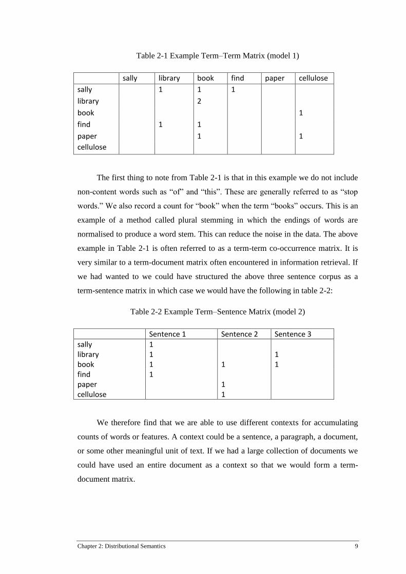
Table 2-1 Example Term–Term Matrix (model 1)
sally library book find paper cellulose
sally 1 1 1
library 2
book 1
find 1 1
paper 1 1
cellulose
The first thing to note from Table 2-1 is that in this example we do not include
non-content words such as “of” and “this”. These are generally referred to as “stop
words.” We also record a count for “book” when the term “books” occurs. This is an
example of a method called plural stemming in which the endings of words are
normalised to produce a word stem. This can reduce the noise in the data. The above
example in Table 2-1 is often referred to as a term-term co-occurrence matrix. It is
very similar to a term-document matrix often encountered in information retrieval. If
we had wanted to we could have structured the above three sentence corpus as a
term-sentence matrix in which case we would have the following in table 2-2:
Table 2-2 Example Term–Sentence Matrix (model 2)
Sentence 1 Sentence 2 Sentence 3
sally 1 library 1 1 book 1 1 1 find 1 paper 1 cellulose 1
We therefore find that we are able to use different contexts for accumulating
counts of words or features. A context could be a sentence, a paragraph, a document,
or some other meaningful unit of text. If we had a large collection of documents we
could have used an entire document as a context so that we would form a term-
document matrix.
10 Chapter 2: Distributional Semantics
One may also make the observation that if there are very many unique words
then the matrix from Table 2-1 will become very large. Likewise, if there are very
many sentences or documents then the matrix from Table 2-2 will become very
large. For millions of unique words, or millions of documents, computing the
semantic model may consume a very large amount of memory. There may also be a
lot of noise contained within the matrix that actually hinders our ability to make good
comparisons between words. This observation leads us to the realization that some
sort of dimensional reduction may be required that will allow us to compress the
information into a smaller space, hopefully retaining the most important information.
The “important” information would obviously be something that would need to be
determined. One approach would be to retain the information which is most
discriminatory, that is, the information that is most useful for identifying differences
in the distributional profile of words.
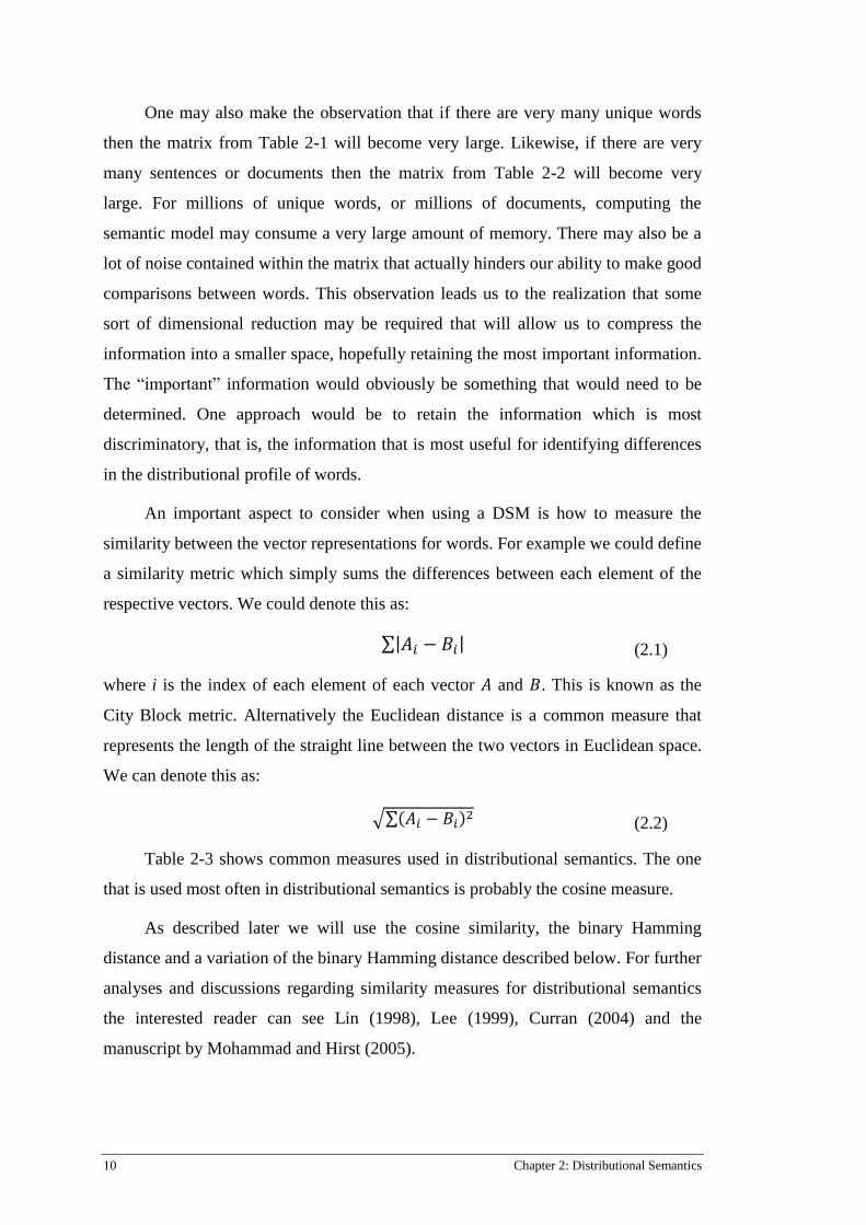
An important aspect to consider when using a DSM is how to measure the
similarity between the vector representations for words. For example we could define
a similarity metric which simply sums the differences between each element of the
respective vectors. We could denote this as:
∑| |
where i is the index of each element of each vector and . This is known as the
City Block metric. Alternatively the Euclidean distance is a common measure that
represents the length of the straight line between the two vectors in Euclidean space.
We can denote this as:
√∑( )
Table 2-3 shows common measures used in distributional semantics. The one
that is used most often in distributional semantics is probably the cosine measure.
As described later we will use the cosine similarity, the binary Hamming
distance and a variation of the binary Hamming distance described below. For further
analyses and discussions regarding similarity measures for distributional semantics
the interested reader can see Lin (1998), Lee (1999), Curran (2004) and the
manuscript by Mohammad and Hirst (2005).
(2.1)
(2.2)

Chapter 2: Distributional Semantics 11
Table 2-3 Distance Measures
Euclidean √∑( ) City Block ∑| |
Cosine
∑
√∑ ∑
Kullback-Leibler
Divergence ∑ (
)
Binary Hamming popCount
(A XOR B) Hellinger ∑(√ √ )
In the definition for the binary Hamming distance given in Table 2-3,
“popCount” refers to a function which counts the number of bits set to “1”.
2.2 PARADIGMATIC VERSUS SYNTAGMATIC
There is an important distinction that we can make between the similarity
relations that we can build from the previous model in Table 2-1 (model 1) and those
that we can build from the previous model in Table 2-2 (model 2). If we take vectors
from model 1, and compare them, we find words that are similar to each other in
such a way that they are able to be substituted for each other. They can be substituted
for each other because they typically occur in similar contexts to each other. They do
not necessarily, however, co-occur together. This type of semantic relation is called
paradigmatic.
Another type of semantics is exemplified in model 2 in which words that have
vectors that are similar to each other are words that often co-occur within the same
context, such as a sentence. This type of semantics is called syntagmatic.
In this thesis we will be focusing on paradigmatic relations between words, i.e.
term-term matrices. For comprehensive analyses of the distinction between
syntagmatic and paradigmatic and its use within DSMs see Rapp (2002) and
Sahlgren (2006).
2.3 PARAMETERS AND DEFINITIONS
The parameters space for distributional semantic models is quite large. We
have highlighted some of these above, such as, window size, choice of context, to

12 Chapter 2: Distributional Semantics
use stop words or not etc. Many options have been explored. Amongst the best
summaries and analyses of the different options in terms of parameters are the papers
by Bullinaria and Levy (2007) and Bullinaria and Levy (2012).
If we were to accumulate all of the parameters for a distributional semantic
model that we have identified up till now in our simple model we would have the
following list:
o Window size (e.g. 5 words either side of target word) for
paradygmatic relations.
o Choice of Context – sentence, document etc. for paradigmatic
relations.
o Include or not include stop words.
o Stemming or lemmatization, e.g. Plural stemming.
o Dimensionality reduction or compression of the resultant statistics.
o Different ways of measuring the distance between vectors.
2.4 HYPERSPACE ANALOGUE TO LANGUAGE
In 1996, Lund and Burgess described a framework (Lund & Burgess 1996) in
which the occurrence of words in a window of 10 words surrounding each target
word are counted and weighted in a way which is inversely proportional to its
distance from the target word. By moving the window over the corpus in one word
increments, and counting co-occurrence statistics, a co-occurrence matrix can be
formed. The matrix actually records words that appear before and after the target
word and in so doing introduces some degree of order information. Various types of
dimensional reduction or feature selection may then be performed and various
measures of similarity used.
HAL was shown to be able to demonstrate semantic categorization,
grammatical categorization such as between different parts of speech, as well as
various semantic priming effects (Burgess, 1998).
The HAL model is actually presented as a high dimensional memory model
which is theoretically not limited to linguistic data but has more general applicability.

Chapter 2: Distributional Semantics 13
2.5 LATENT SEMANTIC ANALYSIS
In an important paper in the field Landauer & Dumais (Landauer & Dumais
1997), demonstrated, using a method called Latent Semantic Analysis (LSA), how
simple word co-occurrence data was sufficient to simulate the growth in a
developing child’s vocabulary. Using 30,473 articles designed for children from
Grolier’s Academic American Encyclopaedia they measured context statistics using
a context window with size of the length of each article or of its first 2,000
characters. The statistics were weighted using an entropy weighting scheme and the
300 most significant dimensions were extracted using Singular Value Decomposition
(SVD). SVD decomposes the co-occurrence matrix into the product of three
matrices where and is a diagonal matrix of singular
values. If we let be the diagonal matrix formed by the top k singular values and
and be the matrices produced from choosing the corresponding columns of
and , then the matrix is the matrix of rank k that best approximates the
original matrix according to the Frobenius norm.
Taking only the most significant dimensions of the SVD is called truncated
SVD. Landauer and Dumais describe truncated SVD as a method for discovering
higher-order co-occurrence. Higher-order co-occurrence terms are terms that do not
necessarily appear together but appear within similar contexts.
Landauer and Dumais demonstrated their model by using it on the synonym
portion of a Test of English as a Foreign Language (TOEFL). The computational
complexity of LSA is heavily dominated by the SVD operation and is difficult to
scale to large corpora but has been one of the benchmarks in distributional semantics.
2.6 RANDOM INDEXING
Random Indexing (Kanerva, Kristofersson and Holst 2000) (RI) introduced an
effective and scalable method for constructing DSMs from large volumes of text.
The method descends from work by Kanerva on Sparse Distributed Representations
(Kanerva 88, 2000). The method is scalable because it performs a type of implicit
dimensional reduction and it performs this in an incremental fashion. It is one of a
number of dimensionality reduction techniques that are based on the observation that
there are many more nearly orthogonal than truly orthogonal directions in high
dimensional space (Hecht-Nielsen 1994) so that if we project points in a vector space
14 Chapter 2: Distributional Semantics
into a randomly selected subspace of sufficiently high dimensionality, the distances
between the points are approximately preserved (Johnson and Lindenstrauss 1984).
Similar methods include Random Projection (Papadimitriou et al., 1998) and
Random Mapping (Kaski, 1999). Papadimitriou et al., (1998) make the first link
between LSA and Random Projections, with Random Indexing being a form of
Random Projections.
We can express Random Projections in the following way:
where the given matrix M is projected by the random matrix R onto a smaller space
M’ where k < d.
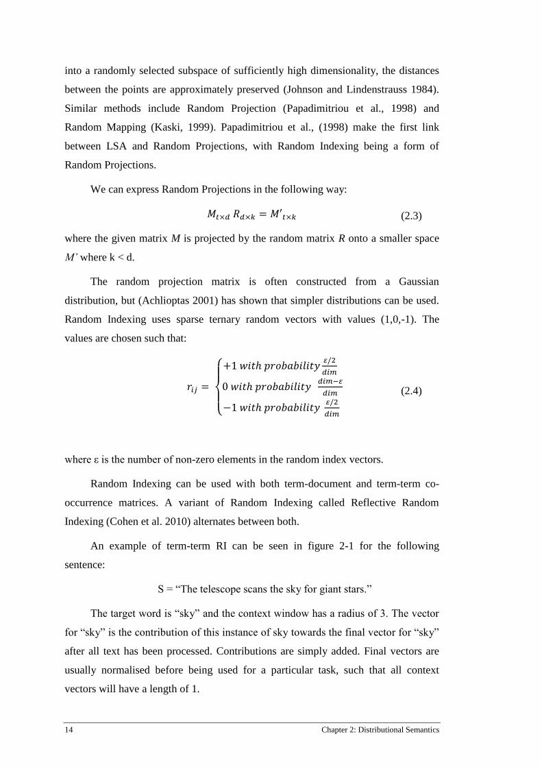
The random projection matrix is often constructed from a Gaussian
distribution, but (Achlioptas 2001) has shown that simpler distributions can be used.
Random Indexing uses sparse ternary random vectors with values (1,0,-1). The
values are chosen such that:
{
where ε is the number of non-zero elements in the random index vectors.
Random Indexing can be used with both term-document and term-term co-
occurrence matrices. A variant of Random Indexing called Reflective Random
Indexing (Cohen et al. 2010) alternates between both.
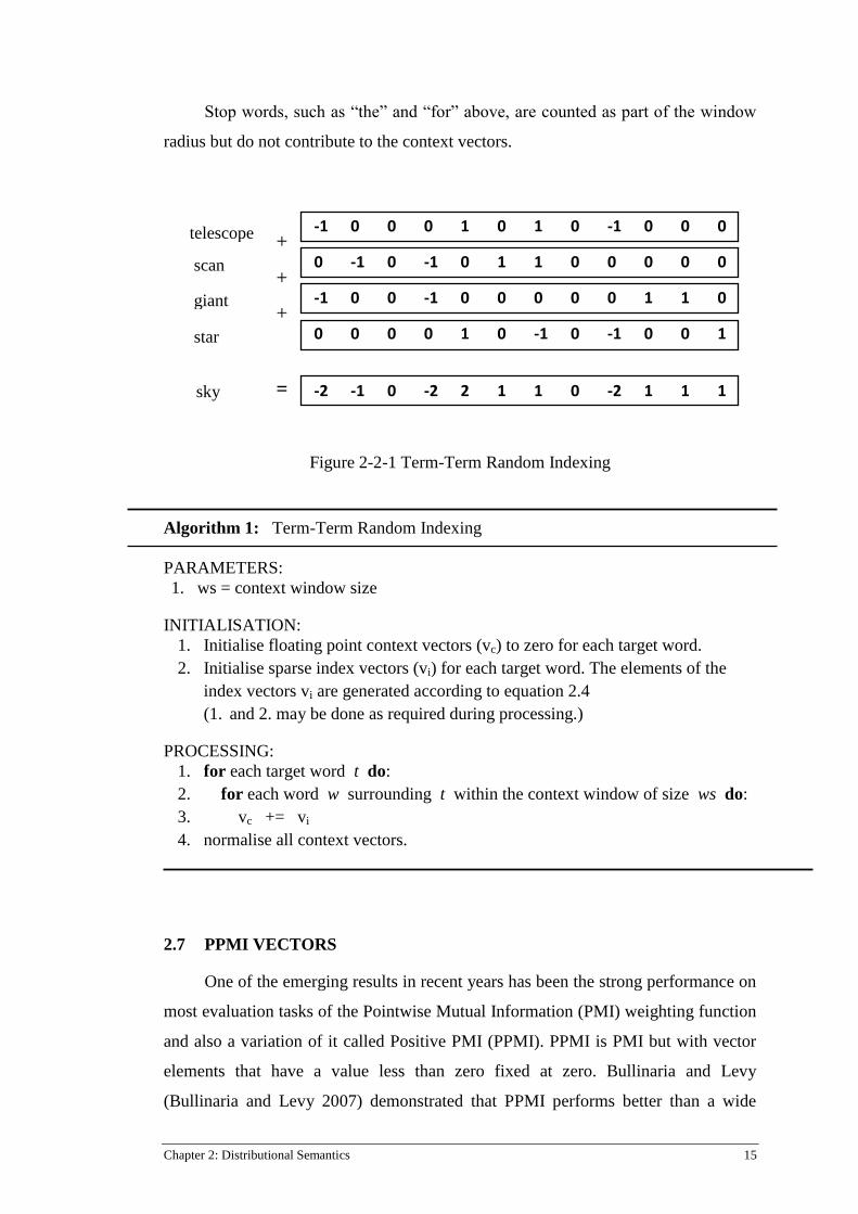
An example of term-term RI can be seen in figure 2-1 for the following
sentence:
S = “The telescope scans the sky for giant stars.”
The target word is “sky” and the context window has a radius of 3. The vector
for “sky” is the contribution of this instance of sky towards the final vector for “sky”
after all text has been processed. Contributions are simply added. Final vectors are
usually normalised before being used for a particular task, such that all context
vectors will have a length of 1.
(2.4)
(2.3)
Chapter 2: Distributional Semantics 15
Stop words, such as “the” and “for” above, are counted as part of the window
radius but do not contribute to the context vectors.
-1 0 0 0 1 0 1 0 -1 0 0 0
0 -1 0 -1 0 1 1 0 0 0 0 0
-1 0 0 -1 0 0 0 0 0 1 1 0
0 0 0 0 1 0 -1 0 -1 0 0 1
-2 -1 0 -2 2 1 1 0 -2 1 1 1
Figure 2-2-1 Term-Term Random Indexing
Algorithm 1: Term-Term Random Indexing
PARAMETERS:
1. ws = context window size
INITIALISATION:
1. Initialise floating point context vectors (vc) to zero for each target word.
2. Initialise sparse index vectors (vi) for each target word. The elements of the
index vectors vi are generated according to equation 2.4
(1. and 2. may be done as required during processing.)
PROCESSING:
1. for each target word t do:
2. for each word w surrounding t within the context window of size ws do:
3. vc += vi
4. normalise all context vectors.
2.7 PPMI VECTORS
One of the emerging results in recent years has been the strong performance on
most evaluation tasks of the Pointwise Mutual Information (PMI) weighting function
and also a variation of it called Positive PMI (PPMI). PPMI is PMI but with vector
elements that have a value less than zero fixed at zero. Bullinaria and Levy
(Bullinaria and Levy 2007) demonstrated that PPMI performs better than a wide
telescope
scan
s giant
star
teles
cop
e
+
+
+
sky =
16 Chapter 2: Distributional Semantics
variety of other weighting approaches when measuring semantic similarity with word
context matrices. PMI is an association measure used extensively in the
psycholinguistic literature and can be traced back to at least Church and Hanks
(1990) who used it for estimating word association norms.
The PMI for a target word t given a context word c is given by:
The context can be a document, sentence or word window. PPMI, as used by
Bullinaria and Levy, is applied to the components of the term vector so that it
becomes a vector of PPMI values indicating the association between the target term
and each of the terms associated with each of the dimensions of the vector.
2.8 BIG DATA, HASHING AND COUNTING
It seems to be generally accepted that having more data to work with in
training a computational model is a good thing, if for no other reason than that one
hopefully has better statistics for the problem domain. Indeed it is also said that more
data beats cleverer algorithms (Recchia & Jones 2009; Domingos 2012). There is a
general trend in scientific research towards greater production and consumption of
data and a consequence of this is that computational methods are required to scale,
both in terms of compute as well as memory resources.
One of the fundamental requirements of distributional semantics is simply to
count the occurrence of features as one processes a given data set. This may seem
like a trivial thing to do until one starts dealing with data sets that no longer fit into
the main memory of one’s computer or that need to be processed in real time. Many
datasets do not match this description, but there are an increasing number that do.
Random Indexing mentioned above is an algorithm that is motivated by the need to
not have to perform large matrix decomposition operations after the statistics have
been collected. It is also incremental and can be updated when more data arrives.
A number of algorithms have been developed in recent years to deal with
scenarios of constrained resources and the need to scale. Some of these are oriented
towards streaming data. Cormode and Muthukrishnan (2005) introduced “Count Min
(𝑐, ) (𝑐 | )
(𝑐) (2.5)
Chapter 2: Distributional Semantics 17
Sketch” for summarizing data streams which allows a number of statistics to be
efficiently calculated on a stream of data without explicitly storing the data. The
method is lossy but has usable accuracy guarantees. This method was later exploited
by Goyal et al. (2010) to accumulate and store statistics for word-context pairs from
90 GB web data in 8 GB of main memory. The word-context pairs are used to
calculate distributional similarity and are applied to a range of word similarity
evaluations. Talbot and Osborne (2007) use a variant of a Bloom Filters (Bloom
1970) to efficiently store corpus statistics and smoothed language models for use in
statistical machine translation. Van Durne and Lall (2009) use a similar approach to
calculate online Pointwise Mutual Information (PMI) scores between verbs in a text
corpus.
Another method called Locality Sensitive Hashing (LSH) (Broder 1997, Indyk
and Motwani 1998) has been used to provide an efficient means to approximate
cosine similarity between high dimensional vectors and has been used for natural
language processing tasks. LSH generates a fingerprint or bit signature which is
much smaller than the original vector but which approximately preserves distance
between the original high dimensional vectors. Ravichandran et al. (2005) use LSH
to generate similarity lists for nouns extracted from a 70 million page web corpus.
Van Durne and Lall (2010) develop a streaming online version of LSH which they
use to calculate distributional similarity across a large text corpus.
2.9 APPLICATIONS OF DISTRIBUTIONAL SEMANTIC MODELS
There are various motivations for wanting to collect statistical information
about language and its use and to encapsulate that information in easy to manipulate
representations. One line of motivation is that such representations are of direct use
in other information technology applications.
Some applications of distributional semantic models in information science
include:
o Information retrieval - The limitations of exact-match keyword-based
information retrieval systems has prompted the use of DSMs for query
expansion and in particular the use of Latent Semantic Indexing (LSI),
with various degrees of success. (Deerwester et al. 1990; Dumais et al.
1995)

18 Chapter 2: Distributional Semantics
o Automatic thesaurus building (Curran & Moens 2002; Grefenstette
1994; Kilgarriff et al. 2004; Lin 1998; Rapp 2004)
o Ontology Learning from text (Buitelaar et al. 2005)
o Application to synonymy tests. (Landauer & Dumais 1997)
o Word sense disambiguation. (Schutze 1998; Yarowsky 1995)
o Bilingual information extraction. (Widdows et al. 2003)
o Information navigation and visualization. (Chen 1999; Widdows
2003; Cohen 2008)
o Entity set expansion – extracting entities from text based on seed
entities. (Pantel et al. 2009)
o Logical inference and applications in Literature Based Discovery
(LBD) (Cole & Bruza 2005; Bruza & Weeber 2008)
.

Chapter 3: Encoding Structure 19
Chapter 3: Encoding Structure
Distributional semantics has often been charged with the failure to incorporate
structured information into its representations of terms. A term – term co-occurrence
matrix, in its simplest form, records statistics about what terms co-occur with what
other terms. It does not take into account the relationship between terms such as their
grammatical relationship or their position with respect to each other in terms of word
order nor the occurrence of bigrams or trigrams etc.
By “structure” we refer to features that are present in the source data and which
are composed of two or more sub-features often with some ordering relationship
defined on them. Structure within a document could be the identification of separate
paragraphs as separate ordered contexts, for example. In lexical semantics it could
the identification of n-grams.
The most common approach in distributional semantics and information
retrieval is to not consider structure. This approach is known as “bag-of-words”
(Harris 1954; Salton & McGill 1983; Joachims 1998). While much of the
information that is available on the World Wide Web is in the form of unstructured
text, there is an increasing trend to tag, annotate and more generally mark-up the
information. This is particularly true with the use of XML and also Semantic Web
technologies which are gradually making inroads into different knowledge domains.
There has been much research in the area of retrieving documents that are
structurally similar or structurally contained within each other, usually in the area of
XML retrieval. Butler (2004) and Tekli et al. (2009) give good summaries. Often a
combination of semantic similarity and structural similarity is used to decide on the
similarity of the given documents.
There is also some history within the Information Retrieval field of trying to
find better representations for documents based on the use of n-grams (particularly
bi-grams) or phrases but there do not seem to be consistent results that convincingly
demonstrate significant improvements as compared to unigram models (Lewis &
Croft, 1990; Bekkerman & Allan 2003); although it depends to some extent on what
the reported baselines are and what the task is. A lot of the work in this area has been
20 Chapter 3: Encoding Structure
applied to text categorization (Fürnkranz 1998; Tan et al. 2004; Bekkerman & Allan,
2004).
Within the field of computational linguistics there has been much work done in
the construction of automated parsers for identifying parts of speech, identifying
dependency relationships between terms, and constructing entire parse trees. This is
in fact a very mature field of research. There has been less work, however, in
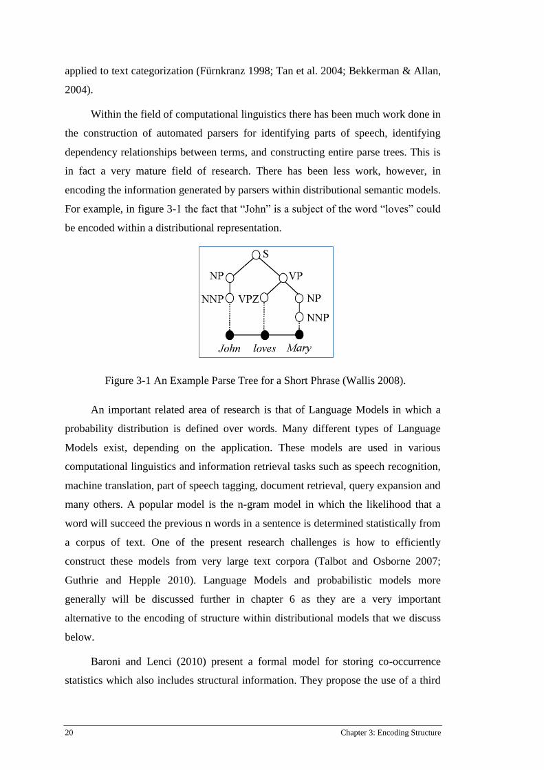
encoding the information generated by parsers within distributional semantic models.
For example, in figure 3-1 the fact that “John” is a subject of the word “loves” could
be encoded within a distributional representation.
Figure 3-1 An Example Parse Tree for a Short Phrase (Wallis 2008).
An important related area of research is that of Language Models in which a
probability distribution is defined over words. Many different types of Language
Models exist, depending on the application. These models are used in various
computational linguistics and information retrieval tasks such as speech recognition,
machine translation, part of speech tagging, document retrieval, query expansion and
many others. A popular model is the n-gram model in which the likelihood that a
word will succeed the previous n words in a sentence is determined statistically from
a corpus of text. One of the present research challenges is how to efficiently
construct these models from very large text corpora (Talbot and Osborne 2007;
Guthrie and Hepple 2010). Language Models and probabilistic models more
generally will be discussed further in chapter 6 as they are a very important
alternative to the encoding of structure within distributional models that we discuss
below.
Baroni and Lenci (2010) present a formal model for storing co-occurrence
statistics which also includes structural information. They propose the use of a third
Chapter 3: Encoding Structure 21
order co-occurrence tensor instead of a co-occurrence matrix. Word-link-word tuples
are stored instead of simply word-word statistics. Baroni and Lenci refer to this
model as a Distributional Memory and as a Structured DSM (distributional semantic
model) as distinct to an unstructured DSM.
Choosing to use “bag-of-words” versus non bag-of-words is basically an issue
of feature selection and/or feature generation.
Bekkerman and Allan (2003) make the observation that feature generation falls
into one of two categories – a) feature combination using disjunction, and b) feature
generation using conjunction. With the first category, features are combined using
disjunctions, such that features are grouped into subsets, then each subset is
considered a new feature. With the second category, features are combined using
only conjunction, for example by grouping close proximity words into phrases. The
use of n-grams as features is an example of this second category. The basic
difference between these two methods is that disjunction decreases statistical
sparseness while conjunction only increases it. This is significant for distributional
semantic models as statistical sparseness often results in noise and is detrimental to
the signal that differentiates one item of interest from another.
3.1 VECTOR SPACE EMBEDDING OF GRAPHS
An area of research that is related to encoding structure within Distributional
Semantic Models is that of vector space embedding of graphs. Graphs can be
embedded within vector spaces to allow more efficient processing, particularly for
graph matching (Riesen et al. 2007). If a target term is represented as a graph with
nodes representing terms and edges representing relationships between terms then
such a model would provide an intuitive means of comparing the similarity of terms.
The similarity measure, however, would generally be computationally demanding.
One approach to reduce the computational complexity is to identify recurring
features and embed the statistics associated with such features within a vector space
for more convenient calculation. This is a complex description of what is done in a
simple way in some of the methods which are described below. The primary
difference between a general graph-based approach and the approach taken in this
thesis is that this thesis is primarily concerned with rather simple structural features,
such as ordered sequences of words, as distinct to the many different complex

22 Chapter 3: Encoding Structure
structures that may be represented using a graph. Graph matching and retrieval is a
very large topic of research and is outside the scope of this thesis. See Luo et al.
(2003) and Spillman et al. (2006) for further work on vector space embedding of
graphs.
3.2 VECTOR SYMBOLIC ARCHITECTURES
The term “Vector Symbolic Architectures” was coined by Gayler (Gayler
2003) to cover a family of related approaches that have grown out of the neural
networks community. These approaches share the property of having algebraic
operations defined on distributed representations over high dimensional vectors.
VSAs originated from Smolenksy’s tensor-product based approach (Smolensky
1990), but differ from it in that they use vector operations that produce products
having the same dimensionality as the component vectors. They can directly
implement functions usually taken to form the kernel of symbolic processing
(Gayler, 1998; Kanerva, 1997; Plate, 1994; Rachkovskij & Kussul 2001). They are
an attempt to incorporate recursive structure into distributed representations and to
provide a link between symbolic and sub-symbolic approaches to representation.
VSA’s differ from other methods of embedding structure within vectors by also
defining an inverse operation which may be used to retrieve noisy versions of object
representations that have been bound into the combined representation. A related
method is that of “Matrix Models” which have been used to model ordered word
associations in human memory (e.g., Humphreys, Bain, & Pike 1989).
Holographic Reduced Representations (HRR) (Plate 1994) is a type of VSA
which is used in the BEAGLE model, described below, to encode word order in a
fully distributed vector representation. They can be used to bind vectors together
without increasing the dimensionality of the resultant vector. This is accomplished
by compressing the outer product of the two bound vectors into a third vector via the
operation of circular convolution. In figure 3-2 below we see the outer product of the
two vectors x and y. The outer product forms a square matrix given that x and y have
the same dimensionality. The circular convolution of x and y is formed by adding all
the elements along a circular path traced over the outer product matrix. For example,
the result of the circular convolution of x and y is z where:

Chapter 3: Encoding Structure 23
z0 = x1y2 + x2y1 + x0y0
z1 = x2y2 + x1y0 + x0y1
z2 = x2y0 + x1y1 + x0y2
Figure 3-2 The Circular Convolution of two vectors defined using paths traced across
the outer product of the two vectors x and y.
Circular convolution is both commutative and associative (equations 3.1, 3.2).
As the operation is commutative it does not record the ordering of the two vector
operands. If non-commutativity is required then one of the vectors may be permuted
before being bound.
( ) ( )
In equations 3.1 and 3.2, indicates circular convolution.
Circular convolution also has an inverse operation called correlation, indicated
by , which can be used to reconstruct a noisy version of one of the convolved
vectors.
𝑐 𝑐
Plate describes many different ways that HRRs can be used to encode
sequences, frames and role/filler structures, including sentences.
HRRs offer several advantages over other representations. They have fixed size
dimensions which do not grow, they degrade gracefully, and they accommodate
arbitrary variable binding (Plate 1994).
It is also claimed that HRRs are neurologically plausible and are used as the
basis for several models of human cognition (Eliasmith & Thagard 2001). A readily
available source for learning about HRRs is Plate’s 2003 book “Holographic
Reduced Representation” (Plate 2003).
(3.1)
(3.3)
Commutativity
Associativity (3.2)
24 Chapter 3: Encoding Structure
3.3 BEAGLE
In language understanding, syntax and semantics play complementary roles.
One generally needs to identify the relations between words in order to understand a
given sentence. The relations may be obvious from the meanings of the words in
some cases, but in other cases the relative positions of the words are important.
BEAGLE (Jones & Mewhort 2006), or Bound Encoding of the Aggregate
Language Environment, is one of the more recent examples of a computational
model of word meaning which seeks to incorporate a notion of structure or syntax.
The major advance offered by BEAGLE is that word representations include both a
consideration of word order information in addition to word context information.
Word order is encoded via the construction and superposition of n-grams.
Given a sequence of symbols S = (s1, s2, s3, …) an n-gram is a n-long
subsequence. The interpretation of the symbols depends on the application area. N-
grams find most application in the areas of computational linguistics, probability
theory and computational biology. Within computational linguistics an n-gram may
be a sequence of letters, a sequence of phonemes or a sequence of words.
In BEAGLE, representations for n-grams are constructed using HRRs. By way
of illustration, assume that the word “old” is represented by a vector and the word
“house” is be represented by the vector . The association between these words,
“old house”, can be represented as a third vector which is the result of the circular
convolution of and , as in Figure 3-2 above. The vectors and are randomly
initialised environmental vectors which fulfil the same role as the index vectors of
Random Indexing. The key difference is that environmental vectors are dense, not
sparse. The environmental vectors are randomly initialised at the start of the
program.
Because the circular convolution operation is commutative (equation 3.1), a
permutation of the elements of one of the bound vectors is employed so that
information about the ordering of words within an n-gram is retained. The
permutation operator is defined randomly at the start of the program. This scheme
can be generalized into representing arbitrarily long sequences of words. Jones &
Mewhort’s original BEAGLE model generates all n-grams up to 7-grams which
overlap the target word. A random placeholder vector Ф is defined to stand in for the
Chapter 3: Encoding Structure 25
target word when the vectors for words are bound together. All the vectors
constructed for n-grams overlapping the target word are accumulated into the
structure (order) vector for the target word. The structure memory for each target
word is thereby constructed as text is processed.
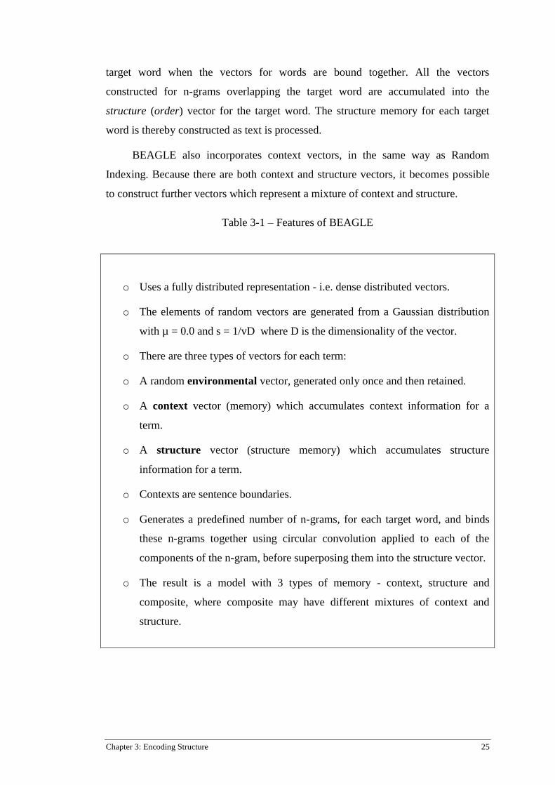
BEAGLE also incorporates context vectors, in the same way as Random
Indexing. Because there are both context and structure vectors, it becomes possible
to construct further vectors which represent a mixture of context and structure.
Table 3-1 – Features of BEAGLE
o Uses a fully distributed representation - i.e. dense distributed vectors.
o The elements of random vectors are generated from a Gaussian distribution
with µ = 0.0 and s = 1/vD where D is the dimensionality of the vector.
o There are three types of vectors for each term:
o A random environmental vector, generated only once and then retained.
o A context vector (memory) which accumulates context information for a
term.
o A structure vector (structure memory) which accumulates structure
information for a term.
o Contexts are sentence boundaries.
o Generates a predefined number of n-grams, for each target word, and binds
these n-grams together using circular convolution applied to each of the
components of the n-gram, before superposing them into the structure vector.
o The result is a model with 3 types of memory - context, structure and
composite, where composite may have different mixtures of context and
structure.

26 Chapter 3: Encoding Structure
For example:
To generate the structure vector for B in the sentence A B C D:
Where:
Π1 is permutation operator 1
Π2 is permutation operator 2
circular convolution
Ф = placeholder random vector for the target word. This vector takes the place
of “__” in the examples below.
We form n-grams and bind them as follows:
BindB,1 = Π1(A) Π2(Ф) A __
BindB,2 = Π1(Ф) Π2(C) __ C
BindB,3 = Π1( Π1(A) Π2(Ф) ) Π2(C) A __ C
BindB,4 = Π1( Π1(Ф) Π2(C) ) Π2(D) __ C D
BindB,5 = Π1( Π1( Π1(A) Π2(Ф)) Π2(C)) Π2(D) A __ C D
We then accumulate the bound n-grams into the structure vector for B.
Algorithm 2: BEAGLE
PARAMETERS:
1. dim = dimension of context vectors
2. nc = maximum number of n-grams to encode.
INITIALIZATION:
1. Randomly initialise dense floating point environmental vectors for each unique
word.
2. Initialise dense floating point context vectors for each unique target word to 0.
3. Initialise dense floating point structure vectors for each unique target word to 0.
(1, 2 and 3 may be done as required during processing.)
Chapter 3: Encoding Structure 27
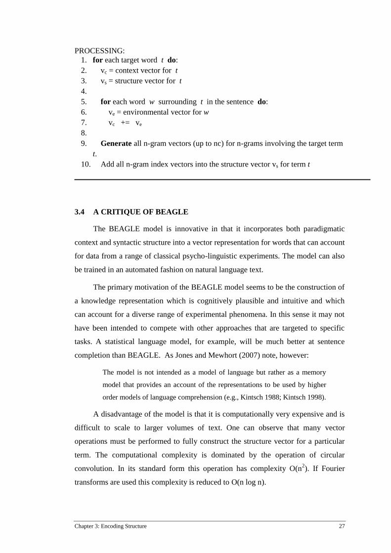
PROCESSING:
1. for each target word t do:
2. vc = context vector for t
3. vs = structure vector for t
4.
5. for each word w surrounding t in the sentence do:
6. ve = environmental vector for w
7. vc += ve
8.
9. Generate all n-gram vectors (up to nc) for n-grams involving the target term
t.
10. Add all n-gram index vectors into the structure vector vs for term t
3.4 A CRITIQUE OF BEAGLE
The BEAGLE model is innovative in that it incorporates both paradigmatic
context and syntactic structure into a vector representation for words that can account
for data from a range of classical psycho-linguistic experiments. The model can also
be trained in an automated fashion on natural language text.
The primary motivation of the BEAGLE model seems to be the construction of
a knowledge representation which is cognitively plausible and intuitive and which
can account for a diverse range of experimental phenomena. In this sense it may not
have been intended to compete with other approaches that are targeted to specific
tasks. A statistical language model, for example, will be much better at sentence
completion than BEAGLE. As Jones and Mewhort (2007) note, however:
The model is not intended as a model of language but rather as a memory
model that provides an account of the representations to be used by higher
order models of language comprehension (e.g., Kintsch 1988; Kintsch 1998).
A disadvantage of the model is that it is computationally very expensive and is
difficult to scale to larger volumes of text. One can observe that many vector
operations must be performed to fully construct the structure vector for a particular
term. The computational complexity is dominated by the operation of circular
convolution. In its standard form this operation has complexity O(n2). If Fourier
transforms are used this complexity is reduced to O(n log n).
28 Chapter 3: Encoding Structure
Results from BEAGLE demonstrate that in some circumstances some
improvement is attained by including order information on evaluation tasks such as
TOEFL.
Because of its use of the binding operation to bind constituent terms together,
BEAGLE has also had some impact on the research area of semantic composition.
Mitchell and Lapata (2008) empirically evaluate a wide range of models for semantic
compositionality, including the use of circular convolution as used in BEAGLE.
3.5 PERMUTATION FOR ENCODING WORD ORDER
In 2008 Sahlgren et al. (2008) introduced a simple and efficient method
inspired by BEAGLE for encoding word order in text which combines Random
Indexing and the use of permutation operators. A permutation is defined for each
word position relative to a target word. Rotations of vector elements are sufficient for
such permutations. For example, a word one place to the left of the target word
would have its index vector rotated to the left one place and then added into the
context vector for the target word. This in effect binds the index word to the position
one place to the left of the target word.
Sahlgren et al. (2008) do not add the representations for stop words into the
structure vector. The stop words tend to add unwanted noise to the representation.
The stop words could be included if desired however.
Let us revisit our example from chapter 2:
S = “The telescope scans the sky for giant stars.”
Becomes: telescope scans sky giant stars (without stop words)
Context vector for sky = Π-2
(telescope) + Π-1
(scan) + Π1 (giant) + Π
2 (star)
where Π-n
indicates a rotation n places.
This method is very efficient and scales very well as the method uses sparse
vectors and does not explicitly generate representations for n-grams. Because index
terms are bound to their position before or after the target term, and are not bound
together to form n-grams, a less specific type of information is added into the context
vectors, as compared with the n-gram binding approach used in BEAGLE.
Chapter 3: Encoding Structure 29
Permutation can also be used to create direction vectors in which case all index
terms before the target term have their vectors permuted (rotated) one way and all
index terms after the target term have their vectors rotated another way. This method
records information about whether a term occurs before or after the target term, but
not in which position it occurred.
Sahlgren et al. use a frequency threshold of 15 000 occurrences of a term for
defining stop words and apply their method to the TOEFL test using a
morphologically normalized form of the TASA corpus. They found that direction
vectors performed best, even better than order and the combined context and
direction vectors.
In this thesis we will refer to this method as Permutation Random Indexing
(PRI).
3.6 SOME OTHER APPLICATIONS OF PERMUTATION RANDOM
INDEXING
In (Cohen et al. 2009), a method called predication-based Semantic Indexing
(PSI) is introduced which encodes semantic predications derived from MEDLINE by
the SemRep system into a vector space representation. Each predicate is assigned a
permutation which is used to permute the elements of the vector for the predicate’s
object. The vector is then superposed into the vector of the subject. Such a method
can be used to encode and add all the predicate object pairs of a subject. The
encoding is reversible, albeit in a lossy manner. This method is an adaptation of
Sahlgren et al’s permutation model for encoding word order in a term-term semantic
space.
Basile et al. 2011 use Random Indexing with permutation to encode syntactic
dependencies obtained using the MINIPAR (Lin 2003) parser. A permutation
operator is assigned to each type of syntactic dependency and the dependency
relation is encoded into the vector for a term in a similar way to PSI above. This
method is evaluated by performing dependency queries and also by execution on a
semantic compositionality task.

30 Chapter 3: Encoding Structure
3.7 OTHER APPLICATIONS USING HOLOGRAPHIC REDUCED
REPRESENTATIONS
There have been several other uses of HRRs within the distributional semantics
and information retrieval domains. Fishbein and Eliasmith (2008) use HRRs to bind
term context vectors with part of speech (POS) information before adding the
resultant vectors into a document representation, using tf-idf weighting. The concept
vectors were generated by Random Indexing. They show that their document
representation improves text classification results as compared to a bag-of-concepts
representation.
Cox et al. (2011) use HRRs to build vector representations for word forms and
integrate these into BEAGLE as part of a unified model. They build on work by
Hannagan et al. (2011) by implementing and evaluating a number of previously
proposed word form encodings but using HRRs as the implementation method. By
word form encodings we mean how words are written and spelt. The representations
are evaluated by comparing representation similarities to human response latency
data produced from lexical decision and word naming experiments.
3.8 RESONANCE AND DECODING
Jones and Mewhort (2007) describe two methods by which information may be
retrieved from representations generated by BEAGLE. The first called “decoding”
retrieves an item instance from the learned memory vector for a word and matches it
with all stored environmental vectors. The item retrieved is a noisy version of one of
the environmental vectors and is thus “cleaned up” by equating it with its closest
match. The item is retrieved using the inverse (or approximate inverse) of the
operation that was used to encode it, namely correlation (inverse convolution).
The other method by which information can be retrieved from a representation
is via “resonance”. It is simply stated as the similarity between the representation for
a word and the representation for another word or some combination of
environmental vectors. This is simply the cosine similarity. It is conceptually and
computationally more simple than the “decoding” method.
Each method has its bias in terms of which representations it is more likely to
retrieve and so Jones and Mewhort suggest that both be used together. To the best of
Chapter 3: Encoding Structure 31
our knowledge there is no existing work which systematically analyses and compares
the respective contributions made by “decoding” and “resonance”.
One aspect of the decoding operation which is not used in the context of
distributional semantics but which is used in various models of human memory and
analogical processing is the ability to perform certain global operations on fully
distributed representations, for example see Plate (2000) ,Kanerva (2010), Cohen
(2012).
For this work we only use the “resonance” method.
3.9 BEAGLE VERSUS PERMUTATION RANDOM INDEXING
BEAGLE represents both context and order information in a composite
representation giving a higher fidelity representation to word meaning. Recchia et al.
(2010) compare BEAGLE with Permutation Random Indexing (PRI) as methods to
encode sequential information in vector space models of semantics. The primary
difference between the models is the way in which items are bound together to
encode order information. BEAGLE uses circular convolution to bind very many
term instances together to form n-grams while PRI binds term index/environmental
vectors to term positions before and after the target term using permutation only.
BEAGLE is computationally expensive which is its primary disadvantage. Recchia et
al. (2010) found that PRI had a better information carrying capacity than BEAGLE
when treating both systems as non-recursive associative memories. By non-recursive
we mean that only one structural level of association is encoded. When both systems
were evaluated on the TOEFL test using a Wikipedia subset for training both
performed comparably well. However, because it was not possible to scale BEAGLE
to the entire Wikipedia corpus, it was not possible to compare the two systems on the
larger corpus. With the larger corpus PRI shows a significant performance
improvement, in line with previous studies indicating that more data gives better
results.
3.10 SEMANTIC COMPOSITIONALITY
Although semantic compositionality is not within the scope of this thesis we
wish to make note of some similarities between semantic compositionality and the
different methods of encoding word order in distributional semantics. The overlap
32 Chapter 3: Encoding Structure
between the two lies in the fact that both use operators and various algebras to
construct representations for larger linguistic units from representations for smaller
linguistic units. The motivation for encoding word order within models of
distributional semantics is to capture information that is missed by simply encoding a
“bag of words.” It is hoped that this extra information is then found to be
advantageous on various tasks as compared to using a “bag of words” representation.
Semantic compositionality, however, is more ambitious than this. It seeks to
build representations and operators for working on them that can be used to directly
construct meaningful representations of complex linguistic statements. See Mitchell
and Lapata (2008), Clark and Pulman (2007), Erk and Padó (2008) and Grefenstette,
Sadrzadeh, Clark, Coecke, and Pulman (2010).

Chapter 4: Extensions to Existing Models 33
Chapter 4: Extensions to Existing Models
In this chapter we present several contributions to the representation and
encoding of structure for distributional semantic models, with specific attention on
word order, and which will be evaluated in chapter 6.
The contributions are as follows:
o Application of Tony Plate’s Holographic Reduced Representations in
the frequency (complex) domain to distributional semantic models.
Some of this work has been published in De Vine and Bruza (2010).
o Experiments with quantisation of real and complex vectors for
distributional semantics.
o The introduction of a variation of random indexing which we call
Structured Random Indexing (SRI) in which a method is defined for
creating sparse index vectors for composed features such as n-grams.
4.1 COMPLEX VECTORS AND DISTRIBUTIONAL SEMANTICS
As previously noted, one of the disadvantages of BEAGLE is its computational
complexity. There are several reasons for this complexity:
o Structure is encoded within vectors using circular convolution which,
with Fourier Transforms, is an O(n log n) operation.
o The vectors used by BEAGLE are dense.
o In the standard BEAGLE model, very many convolution operations
are required per target term, particularly when up to 7-grams are
encoded.
Using Holographic Reduced Representations (HRR) in the frequency domain
(complex plane) is one method to reduce the compute time of BEAGLE. It reduces
the compute time of the binding operation from O(n log n) to O(n). This makes a
difference for high dimensional vectors. In chapter four of his thesis (Plate 1994)
Plate describes how one may compute and use HRRS in the frequency domain. He
refers to this system also as the circular system. We will refer to them in this thesis as

34 Chapter 4: Extensions to Existing Models
Circular Holographic Reduced Representations (CHRR). CHRRs have the same
important properties as HRRs with a few differences relating to less important
properties such as the absence of a zero vector (see Table 4-1 below).
Complex valued vectors have predominantly found application in signal
processing and electronics, physics (esp. electromagnetism and quantum mechanics),
and to a lesser extent in machine learning (complex valued neural networks). The
primary reason that complex numbers are relevant for this thesis is that complex
numbers provide an efficient way to compute the circular convolution of two vectors.
They are also of conceptual interest as they can provide a unifying model for the
different types of Vector Symbolic Architectures previously mentioned (Kanerva
2009; Aerts 2009).
Although complex numbers can be represented as an ordered pair of real
numbers, they gain their unique character by virtue of the way that complex
multiplication is defined.
We can represent a complex number z as z ≡ (x,y) where x and y are real
numbers. Addition and multiplication of z1 and z2 are defined as:
(x1,y1)+(x2,y2) ≡ (x1+x2, y1+y2)
(x1,y1).(x2,y2) ≡ (x1x2 – y1y2, x1y2 + y1x2)
Complex multiplication has a rotational component in which points in the
complex plane are rotated with respect to each other when multiplied together. When
points lie on the complex unit circle multiplication is equivalent to the addition of the
phase angles of each of the two operands.
Table 4-1 Respective Entities and Operations for HRRs and CHRRs (Based on
the table from Plate 1994)
Entity/Operation HRRs CHRRs
Random vector Elements iid as
N( , ) Elements iid as U( , )
Zero vector , , , , , No corresponding object
Superposition Vector addition Angle of sum ( )
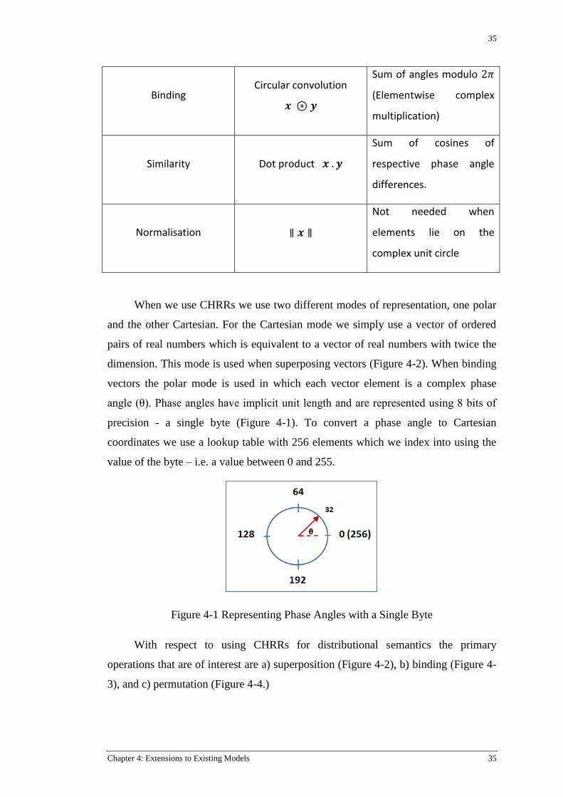
35
Chapter 4: Extensions to Existing Models 35
Binding Circular convolution
Sum of angles modulo
(Elementwise complex
multiplication)
Similarity Dot product
Sum of cosines of
respective phase angle
differences.
Normalisation
Not needed when
elements lie on the
complex unit circle
When we use CHRRs we use two different modes of representation, one polar
and the other Cartesian. For the Cartesian mode we simply use a vector of ordered
pairs of real numbers which is equivalent to a vector of real numbers with twice the
dimension. This mode is used when superposing vectors (Figure 4-2). When binding
vectors the polar mode is used in which each vector element is a complex phase
angle (θ). Phase angles have implicit unit length and are represented using 8 bits of
precision - a single byte (Figure 4-1). To convert a phase angle to Cartesian
coordinates we use a lookup table with 256 elements which we index into using the
value of the byte – i.e. a value between 0 and 255.
Figure 4-1 Representing Phase Angles with a Single Byte
With respect to using CHRRs for distributional semantics the primary
operations that are of interest are a) superposition (Figure 4-2), b) binding (Figure 4-
3), and c) permutation (Figure 4-4.)

36 Chapter 4: Extensions to Existing Models
Figure 4-2 Superposition of Complex
Vector Elements (A + B) in Cartesian
Mode
Figure 4-3 Binding by Circular
Convolution - A * B in Polar Mode
Figure 4-4 Permutation by Rotating One Place to the Left
In CHRRs information is encoded in phase angles. During model training the
phase angles become strongly aligned in different directions as determined by the
random initialization of the environmental/index vectors and the information
contained in the distributional profile of words. When used with BEAGLE the
elements of the memory and structure CHRR vectors are initialised with small
random perturbations from 0 in Cartesian form. These perturbations are quickly
dominated by the superposition of environmental/index vectors, and should an
element not be touched during the learning process, the element will take on the
random phase angle determined by the initial random perturbation.

37
Chapter 4: Extensions to Existing Models 37
At the conclusion of the training session all elements are converted from
Cartesian to Polar representation. In practice this means that a vector of dimension
2n is transformed into a vector of dimension n.
Similarity between vectors is calculated by calculating the average cosine of
the difference between respective phase angles as represented in polar form (Table 4-
1) (See also Plate 1994, chapter 4). A simpler way to calculate similarity is to simply
calculate the average difference between phase angles.
Encoding information in phase angles is a common technique used in
engineering and particularly signal processing. Phase-Shift Keying (PSK) (Bateman
1999) is a well-known method for encoding digital data in an analogue wave.
For more information about the respective merits of CHRRs and HRRs see
chapter four of Plate (1994).
The above work involving the encoding of distributional semantics in complex
vectors has been implemented in both Java and C++. The Java code uses 16 bits to
represent phase angles whereas the C++ version uses 8 bits. The Java version has
been incorporated into the SemanticVectors Java package (Widdows & Ferraro
2008).
4.2 BINARY VECTORS AND QUANTISATION
Binary vectors provide a very compact and efficient representation for many
applications because of the hardware support provided for bitwise operations in
modern computers. Kanerva (2009) gives a very good overview of some of the
possibilities and advantages of computing with very high dimensional bit vectors.
One way to produce binary vectors, or bit vectors, is to simply perform scalar
quantisation on real valued vectors (Figure 4-5). Quantisation is the procedure of
mapping something from a large or continuous set of values to a relatively small set
of discrete values. It is a method that is used extensively in coding theory,
information retrieval and signal processing. Quantisation was recently used by (Geva
& De Vries 2011) in a method called TOPSIG to produce bit vector representations
of real valued vectors obtained by random indexing of text documents. Quantisation
of real valued vectors to bit vectors is also often called binarisation. Quantisation

38 Chapter 4: Extensions to Existing Models
may be used to digitize an analogue signal or compress a signal in which case it has
an associated information loss.
Figure 4-5 Quantising to a Bit Vector
When real valued vectors are quantised we use the Hamming distance as the
similarity metric. Quantisation of semantic vectors is one of the options that we
evaluate in this thesis for two reasons: a) we are not aware of other reported results
that do exactly this, i.e. binarise real valued vectors for term representation, although
there are a number of similar methods that use bit vectors which we mention below;
b) there are a number of useful methods for efficiently retrieving nearest neighbour
bit vectors as distinct to real valued bit vectors. We do not evaluate b) as this is an
extensive topic and is outside the scope of this thesis.
As a quick comment on the efficiency of bit vector representations, if one takes
a real valued vector represented with 32 bit floating point precision and quantises
each element (scalar quantisation) to a single bit, the resultant representation is only
1/32 the size of the original. This is a significant savings but obviously raises the
question regarding what information is lost.
Ravichandran (2005) uses Locality Sensitive Hashing (LSH) (Broder (1997),
Indyk and Motwani, 1998) to map vectors representing nouns into binary fingerprints
which are then used to generate noun similarity lists.
An important work related to quantised vectors is the Binary Spatter Code
(Kanerva 1996) representation which we mention below in relation to HRRs. When
computing with BSCs, bit vectors are superposed and the number of 1s and 0s
accumulated in each dimension are counted and a majority rule is used to set the
resultant bit in each dimension to either a 1 or 0. A tricky aspect of this
representation is how to keep count of the 1s and 0s in each dimension. Cohen et al.
(2012) make innovative use of Lucene’s bitset class to construct an optimised voting
record for implementing the majority rule when working with BSCs. Widdows et al.
(2012) gives a good description of how complex, binary and real valued vectors were
integrated within the SemanticVectors package to form “typed” vectors.
< 0.2, 0.4, -0.2, 0.2, 0.5, -0.3, -0.2, -0.2 > 1 1 0 1 1 0 0 0
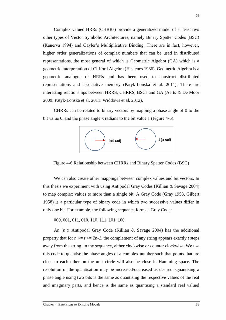
39
Chapter 4: Extensions to Existing Models 39
Complex valued HRRs (CHRRs) provide a generalized model of at least two
other types of Vector Symbolic Architectures, namely Binary Spatter Codes (BSC)
(Kanerva 1994) and Gayler’s Multiplicative Binding. There are in fact, however,
higher order generalizations of complex numbers that can be used in distributed
representations, the most general of which is Geometric Algebra (GA) which is a
geometric interpretation of Clifford Algebra (Hestenes 1986). Geometric Algebra is a
geometric analogue of HRRs and has been used to construct distributed
representations and associative memory (Patyk-Lonska et al. 2011). There are
interesting relationships between HRRS, CHRRS, BSCs and GA (Aerts & De Moor
2009; Patyk-Lonska et al. 2011; Widdows et al. 2012).
CHRRs can be related to binary vectors by mapping a phase angle of 0 to the
bit value 0, and the phase angle π radians to the bit value 1 (Figure 4-6).
Figure 4-6 Relationship between CHRRs and Binary Spatter Codes (BSC)
We can also create other mappings between complex values and bit vectors. In
this thesis we experiment with using Antipodal Gray Codes (Killian & Savage 2004)
to map complex values to more than a single bit. A Gray Code (Gray 1953, Gilbert
1958) is a particular type of binary code in which two successive values differ in
only one bit. For example, the following sequence forms a Gray Code:
000, 001, 011, 010, 110, 111, 101, 100
An (n,t) Antipodal Gray Code (Killian & Savage 2004) has the additional
property that for n <= t <= 2n-1, the complement of any string appears exactly t steps
away from the string, in the sequence, either clockwise or counter clockwise. We use
this code to quantise the phase angles of a complex number such that points that are
close to each other on the unit circle will also be close in Hamming space. The
resolution of the quantisation may be increased/decreased as desired. Quantising a
phase angle using two bits is the same as quantising the respective values of the real
and imaginary parts, and hence is the same as quantising a standard real valued

40 Chapter 4: Extensions to Existing Models
vector. The ability to easily adjust the level of quantisation allows for easily
experimenting with the trade-off between representation size and information
content.
For example, using 4 bits, we can quantise phase angles using the mapping in
figure 4-7. A quantised result is shown in figure 4-8.
Figure 4-7 A 4 Bit Antipodal Gray Code
Figure 4-8 A Two Element Vector of Phase Angles Quantised Using an Antipodal
Gray Code
4.3 SPARSE ENCODING OF STRUCTURE AND STRUCTURED
RANDOM INDEXING
We would like to be able to construct a model for encoding structure in
distributional semantics which is simpler than BEAGLE but retains the ability to
encode specific information about n-grams. We now propose a method which we call
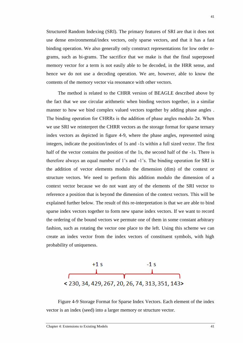
41
Chapter 4: Extensions to Existing Models 41
Structured Random Indexing (SRI). The primary features of SRI are that it does not
use dense environmental/index vectors, only sparse vectors, and that it has a fast
binding operation. We also generally only construct representations for low order n-
grams, such as bi-grams. The sacrifice that we make is that the final superposed
memory vector for a term is not easily able to be decoded, in the HRR sense, and
hence we do not use a decoding operation. We are, however, able to know the
contents of the memory vector via resonance with other vectors.
The method is related to the CHRR version of BEAGLE described above by
the fact that we use circular arithmetic when binding vectors together, in a similar
manner to how we bind complex valued vectors together by adding phase angles .
The binding operation for CHRRs is the addition of phase angles modulo 2π. When
we use SRI we reinterpret the CHRR vectors as the storage format for sparse ternary
index vectors as depicted in figure 4-9, where the phase angles, represented using
integers, indicate the position/index of 1s and -1s within a full sized vector. The first
half of the vector contains the position of the 1s, the second half of the -1s. There is
therefore always an equal number of 1’s and -1’s. The binding operation for SRI is
the addition of vector elements modulo the dimension (dim) of the context or
structure vectors. We need to perform this addition modulo the dimension of a
context vector because we do not want any of the elements of the SRI vector to
reference a position that is beyond the dimension of the context vectors. This will be
explained further below. The result of this re-interpretation is that we are able to bind
sparse index vectors together to form new sparse index vectors. If we want to record
the ordering of the bound vectors we permute one of them in some constant arbitrary
fashion, such as rotating the vector one place to the left. Using this scheme we can
create an index vector from the index vectors of constituent symbols, with high
probability of uniqueness.
Figure 4-9 Storage Format for Sparse Index Vectors. Each element of the index
vector is an index (seed) into a larger memory or structure vector.

42 Chapter 4: Extensions to Existing Models
Each compressed SRI index vector associated with a base word is randomly
generated (just like RI), while making sure that no element value is duplicated.
Duplication is avoided so that there is no collision of 1s or -1s.
Because each element of an index vector is independent of all other elements,
and no checks are made for duplication during the binding process, it is possible for
two elements to have the same value, depending on the sparsity of the index vectors.
This may lead to a +1 or -1 being added to the same location in the full memory
vector as another +1 or -1. We are forced to accept this as an inherent side-effect of
our method and our observations are that it does not significantly affect results. If
desired, however, corrections can be made to the bi-gram index vector to remove
duplications, with some effect on performance. We investigate the bias that this side-
effect introduces in section 4.4.
Figure 4-10 shows an example of operations on the vectors A and B. Line 4
shows A B which is the element-wise addition modulo 512 of A and B. We take
512 to be the dimensionality of the full context vector. Line 5 shows A bound with a
permuted B in which case the binding operation becomes non-commutative.
(1) A = < 230, 34, 429, 267, 20, 26, 74, 313, 351, 143 >
(2) B = < 42, 129, 312, 211, 30, 505, 303, 198, 15, 7 >
(3) Π-1
(B) = < 129, 312, 211, 30, 505, 303, 198, 15, 7, 42>
(4) A B = < 272, 163, 229, 478, 50, 19, 377, 511, 366, 150 > = B A
(5) A Π-1
(B) = < 359, 346, 128, 297, 13, 329, 272, 328, 358, 185 > ≠ B A
Figure 4-10 Creating Sparse Index Vectors by Composition – Commutative
and Non-Commutative
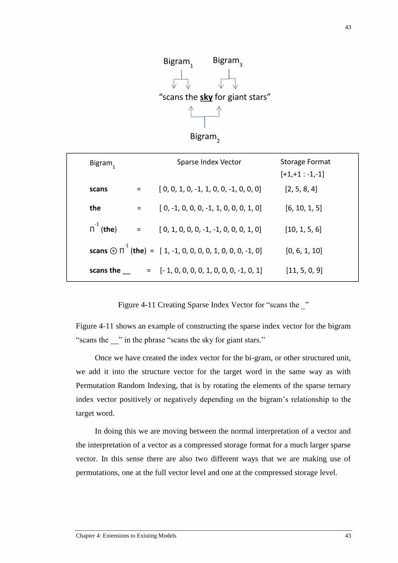
43
Chapter 4: Extensions to Existing Models 43
Figure 4-11 Creating Sparse Index Vector for “scans the _”
Figure 4-11 shows an example of constructing the sparse index vector for the bigram
“scans the __” in the phrase “scans the sky for giant stars.”
Once we have created the index vector for the bi-gram, or other structured unit,
we add it into the structure vector for the target word in the same way as with
Permutation Random Indexing, that is by rotating the elements of the sparse ternary
index vector positively or negatively depending on the bigram’s relationship to the
target word.
In doing this we are moving between the normal interpretation of a vector and
the interpretation of a vector as a compressed storage format for a much larger sparse
vector. In this sense there are also two different ways that we are making use of
permutations, one at the full vector level and one at the compressed storage level.
Bigram1 Bigram
3
scans = [ 0, 0, 1, 0, -1, 1, 0, 0, -1, 0, 0, 0] [2, 5, 8, 4] the = [ 0, -1, 0, 0, 0, -1, 1, 0, 0, 0, 1, 0] [6, 10, 1, 5]
Π-1
(the) = [ 0, 1, 0, 0, 0, -1, -1, 0, 0, 0, 1, 0] [10, 1, 5, 6]
scans Π-1
(the) = [ 1, -1, 0, 0, 0, 0, 1, 0, 0, 0, -1, 0] [0, 6, 1, 10] scans the __ = [- 1, 0, 0, 0, 0, 1, 0, 0, 0, -1, 0, 1] [11, 5, 0, 9]
Sparse Index Vector Storage Format
[+1,+1 : -1,-1]
“scans the sky for giant stars”
Bigram2
Bigram1
44 Chapter 4: Extensions to Existing Models
Using this method we can create sparse index vectors for arbitrary structural
elements. In this thesis we construct index vectors for bi-grams, both ordered and
unordered, but other types of structured information could easily be encoded.
The primary advantage of this method is efficiency. We can encode very
specific information very quickly because we only use sparse index vectors. There is
also no problem of encoding frequently occurring words as part of the n-gram, such
as stop-words, as these will not dominate the memory vector as in the case with PRI.
Another, but very different, method that defines a binding operation on sparse
vectors is Context Dependent Thinning (Rachkovskij and Kussul 2001). It defines a
binding operation on sparse binary vectors while also retaining sparsity. It has
different properties from SRI, however, in that it tries to maintain similarity between
the resultant vector and the composed vectors.
4.4 ANALYSIS OF BIAS IN SRI INDEX VECTORS
We remember that a seed is the value of an element in a compressed storage
index vector which represents a position in the expanded sparse vector. The number
of seeds determines the sparsity of the sparse index vector which it encodes. We can
determine the average number of seeds that will collide per vector when using the
SRI method, assuming uniform random placement, using the following:
dim = dimension of memory vector
ns = number of seeds
( )
The average number of seeds colliding when ns seeds are allocated values in
[1, dim] is approximately the probability that the first seed will collide (0), plus the
probability that the second seed will collide, plus the probability that the third seed
will collide, etc.
For simplicity we approximate this as:
For example if we have dim = 4096 and ns = 32, then
(4.1)
(4.2)
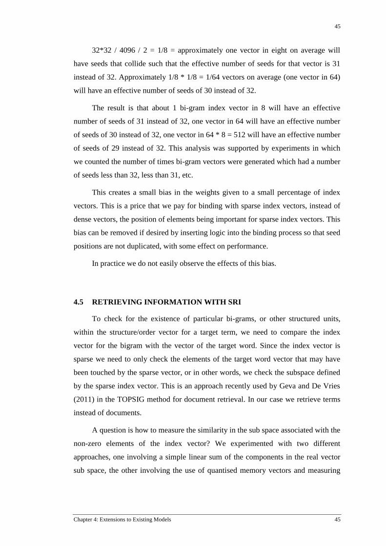
45
Chapter 4: Extensions to Existing Models 45
32*32 / 4096 / 2 = 1/8 = approximately one vector in eight on average will
have seeds that collide such that the effective number of seeds for that vector is 31
instead of 32. Approximately 1/8 * 1/8 = 1/64 vectors on average (one vector in 64)
will have an effective number of seeds of 30 instead of 32.
The result is that about 1 bi-gram index vector in 8 will have an effective
number of seeds of 31 instead of 32, one vector in 64 will have an effective number
of seeds of 30 instead of 32, one vector in 64 * 8 = 512 will have an effective number
of seeds of 29 instead of 32. This analysis was supported by experiments in which
we counted the number of times bi-gram vectors were generated which had a number
of seeds less than 32, less than 31, etc.
This creates a small bias in the weights given to a small percentage of index
vectors. This is a price that we pay for binding with sparse index vectors, instead of
dense vectors, the position of elements being important for sparse index vectors. This
bias can be removed if desired by inserting logic into the binding process so that seed
positions are not duplicated, with some effect on performance.
In practice we do not easily observe the effects of this bias.
4.5 RETRIEVING INFORMATION WITH SRI
To check for the existence of particular bi-grams, or other structured units,
within the structure/order vector for a target term, we need to compare the index
vector for the bigram with the vector of the target word. Since the index vector is
sparse we need to only check the elements of the target word vector that may have
been touched by the sparse vector, or in other words, we check the subspace defined
by the sparse index vector. This is an approach recently used by Geva and De Vries
(2011) in the TOPSIG method for document retrieval. In our case we retrieve terms
instead of documents.
A question is how to measure the similarity in the sub space associated with the
non-zero elements of the index vector? We experimented with two different
approaches, one involving a simple linear sum of the components in the real vector
sub space, the other involving the use of quantised memory vectors and measuring

46 Chapter 4: Extensions to Existing Models
the agreement between the index vector and memory vector in the Hamming sub
space. We show results of the second approach in chapter 6 for completing phrases.
4.6 ENCODING STRUCTURE IN DISTRIBUTIONAL SEMANTICS
When encoding word order in distributional semantics we need to decide on
what order n-grams to limit our model to. A basic observation is that the higher the
order of the n-gram the more specific the information is that is being contributed by
the n-gram. In this thesis we limit the order to two such that only bi-grams are
encoded. The rationale for this is that it allows us to test the usefulness of encoding
structure without adding unnecessary complication. If encoding bi-grams is found to
be useful then higher order n-grams can then be tested.
We therefore limit our implementation of BEAGLE to bi-grams, although we
will still refer to the model as a BEAGLE model since we are still using circular
convolution to bind vectors.
For example, with the phrase “A B _ D E” where “_” indicates the target word,
we will generally construct the bigrams:
Bigram1 A B, Bigram2 B D, Bigram3 D E,
although the C++ implementation is such that a larger variety of bigrams may be
considered.
We do not include unigrams as we incorporate the contribution of unigrams via
mixing a structured model with a non-structured model.
Chapter 5: Experimental Setup 47
Chapter 5: Experimental Setup
Our experimental setup consists of three elements, a) the evaluation tasks and
experiments, b) the text corpora for training, and c) our implementation of the
various computational models.
5.1 EVALUATION TASKS
To evaluate the various contributions we use several evaluation tasks including
the TOEFL test, the WS353 semantic relatedness test, and a semantic space overlap
test. The primary test that we use is the TOEFL. We also use several auxiliary
experiments to better examine the abilities and effectiveness of the different models.
These auxiliary experiments include several methods for examining the nearest
neighbours of a term in a model and also the retrieval of structured information from
a model. These latter auxiliary test are described in more detail in the results section
in chapter 6.
5.1.1 TOEFL
A common evaluation task for semantic models is the synonym section of the
Test of English as a Foreign Language - TOEFL (Landauer & Dumais, 1996, 1997;
Turney, 2001). Each item consists of a target word and four alternative words; the
task is to select the alternative that is most similar in meaning to the target. Accuracy
on a set of 80 items was originally used by Landauer and Dumais (1997) as the
criterion for dimensionality selection in LSA, and the TOEFL has since become a
benchmark for measuring performance of semantic models.
Table 5-1 Example TOEFL Question
1. enormously
a) appropriately
b) uniquely
c) tremendously
d) decidedly

48 Chapter 5: Experimental Setup
Given the extent to which TOEFL is used as an evaluation tool within
distribution semantics the TOEFL will be our primary evaluation task. We will also
analyse the “error profile” on this task for different models to learn more about the
differences between models. To this end we have chosen a subset of 20 questions
which by manual inspection seem to be “problem” questions for different models. As
far as we are aware this is the first time that the error profile has been analysed on the
TOEFL test.
5.1.2 WordSim353
The WordSim353 dataset (WS-353) has been used extensively in recent work
in distributional semantics. Originally collected by Finkelstein et al. (2001), the
dataset consists of 353 word pairs. The degree of relatedness of each pair is assessed
on a 0-10 scale by 13-16 human judges where the average is used as the final score.
Agirre et al. (2009) further split this dataset into similar pairs (WS-sim) and related
pairs (WS-rel), where the former contains synonyms, antonyms, identical words and
hyponyms/hypernyms and the latter captures other word relations.
We use the Spearman correlation to measure the correlation between the
ranked similarities as computed by the semantic model, and the similarities as
elicited from the human judges. The Spearman correlation is preferred over the
Pearson correlation as it can be used to effectively measure the correlation for
variables that have a non-linear relationship.
Table 5-2 Examples of Word Pairs and their Relatedness as Judged by Human
Judges
bread butter 6.19
king cabbage 0.23
journey car 5.85
This task is quite difficult for vector space models as it is not immediately clear
how one should rank the similarity of one pair of words with another pair of words,
given that the significance of the similarity measure may be quite different in
different parts of the vector space, depending on the local geometry of the space. For
example, if the words “red” and “blue” have a cosine similarity of 0.7, is this better
49
Chapter 5: Experimental Setup 49
than a cosine similarity of 0.6 for the terms “bus” and “car”? Nevertheless for this
task we use the raw cosine similarities. Better semantic models generally perform
better on this task.
5.1.3 Semantic Space Overlap
In (Sahlgren 2006) a method is presented to measure the amount of overlap
between two semantic spaces. Sahlgren defines the overlap as the number of shared
words between neighbourhoods in the two spaces. The neighbourhood can be
defined in an absolute sense such as all the words that are within 0.5 cosine
similarity, for example, of a given word are defined as being part of the
neighbourhood of that word, or the neighbourhood can be defined in a relative sense
such that the 10 closest words are considered part of the neighbourhood. Sahlgren
uses the second approach. The given words can be all of the words for which
memory vectors have been generated or a random sample can be taken.
For this task we use the BNC corpus and randomly choose 1000 words from
the target words that we have constructed memory vectors for. We use the nearest 50
words of each given term as the neighbourhood. We found that for constant n nearest
neighbours the computed overlap was quite stable irrespective of which 1000 random
words were chosen.
5.2 CORPORA
To train the various models which we have described previously we make use
of several corpora:
1. Touchstone Applied Science Associates (TASA) corpus.
2. British National Corpus (BNC).
3. Wikipedia INEX 2009. (INEX)
5.2.1 TASA Corpus
The TASA corpus is a collection of text representative of the reading material
that a person is supposed to have been exposed to by their first year in an American
college (Zeno, Ivens, Millard, & Duvvuri, 1995; Landauer, Foltz, & Laham 1998).
It contains short samples from textbooks, works of literature, and popular
works of fiction and nonfiction and contains approximately 10 million words. It has

50 Chapter 5: Experimental Setup
been used extensively to train distributional models in computational linguistics and
cognitive science research (Griffiths et al., 2007; Jones & Mewhort, 2007; Landauer
& Dumais, 1997).
5.2.2 The British National Corpus (BNC)
The British National Corpus (BNC) (BNC XML Edition, 2007) is a 100-
million-word text corpus of samples of written and spoken English. It covers British
English of the late 20th century including a wide variety of genres with the intention
that it be a representative sample of spoken and written British English of that time.
It has been taken from a wide range of sources with approximately 90% being
samples of written language use. Written language was extracted from regional and
national newspapers, published research journals or periodicals from various
academic fields, both fiction and non-fiction books, both published and unpublished
material such as leaflets, brochures, letters, essays written by students of differing
academic levels, speeches, scripts and other types of texts. The spoken samples
making up 10% were presented and recorded in the form of transcriptions. They
consist of a “demographic” part, which represents different age groups, social
classes, etc., and a “context-governed” part which contains transcriptions of
recordings made at specific types of meeting and event.
The BNC corpus has been tagged for grammatical information (part of speech).
The CLAWS4 system was used for tagging the BNC. The tags were not used for the
experiments reported in this thesis.
The BNC has been used extensively for research in computational linguistics
and also for the construction of distributional models of word meaning.
5.2.3 INEX Wikipedia Collection
The INEX Wikipedia collection consists of 50.7 GB of Wikipedia articles in
XML form and contains more than 2.6 million documents.
The documents are enhanced with semantic mark-up of articles and outgoing
links, based on the semantic knowledge base YAGO (Suchanek, Kasneci & Weikum,
2007), which explicitly labels more than 5,800 classes of entities like persons,
movies, cities, and many more. The collection was created from the October 8, 2008
dump of the English Wikipedia. The semantic mark-up is not used in this work but
may be an interesting task for future work.

51
Chapter 5: Experimental Setup 51
After pre-processing there were approximately 750 million terms remaining.
5.3 PRE-PROCESSING
The pre-processing of the corpus text was performed using Java. Each
document was split into a sequence of sentences using the Apache OpenNLP Tools
Java library (Apache OpenNLP. (n.d.)). This library uses a maximum entropy model
and a selection of text for learning how to recognise sentence boundaries. This
library seems to produce good results. All terms were lowercased. Terms containing
numeric characters were replaced with the standard term “nn”. Terms were not
lemmatized and no stemming was used.
The INEX Wikipedia collection required special attention as it contains
elements that do not represent full sentences, such as lists of entities, titles, times and
dates etc. The XML was parsed and only elements matching certain criteria were
extracted so as to produce well-formed sentences. The final INEX corpus contained
approximately 750 million terms.
5.4 TEXT INDEXING
The pre-processed corpora were indexed using the open source C++ search
engine Indri. Indri is a component of the Lemur project (The Lemur Project 2013)
and is a state-of-the-art search engine often used in IR research. Indri is primarily
developed and maintained by the University of Massachusetts and Carnegie Mellon
University.
The idea of using a search engine such as Indri instead of simply processing
plain text files comes from experience with the SemanticVectors package (Widdows
& Ferraro 2008) which is built on top of Lucene. Using a text indexer such as Indri
provides some additional functionality at no extra developmental cost.
A separate index was created for each of the three corpora.
5.5 BASE TERMS AND EVALUATION TERMS
The list of base terms, that is the terms associated with an index or
environmental vector, was generated by taking the terms that occur at least 5 times in
the TASA corpus, and at least 10 times in the BNC corpus. All of the terms that are

52 Chapter 5: Experimental Setup
required for evaluation tasks are then also merged into this list of base terms. This
final list of base terms contained approximately 86 000 terms.
The list of evaluation terms is comprised of all the terms that occur in the
TOEFL task, the WS353 task and some additional terms that occur in a semantic
clustering task which is not reported on in this thesis.
5.6 THE GENERAL WORKFLOW FOR BUILDING MODELS
The general workflow that is used for building vectors from a text corpus is
as follows:
1) Initialise the required vector spaces by allocating memory and initialising
vectors. Process the documents from the Indri index, accumulating
information into the vectors according to the chosen method.
2) Post-process the vectors. This may include one or more of the following:
a) Transformation of vector elements, such as applying PPMI weighting to
full co-occurrence vectors.
b) Normalisation of vectors to unit length.
c) Quantisation of vectors to a bit vector representation.
3) Save the vectors to disk.
5.7 TERM WEIGHTING AND SIMILARITY METRIC
Three different weighting schemes are used for weighting the contribution of
terms to the memory vector:
a) Constant weighting: each vector has weight 1.0.
b) Entropy weighting: ( ∑ ( ))
where n is the number of documents and is the probability of the term i
appearing in the document j. This is a global weighting scheme that is often
used with LSA (Berry & Browne 2005).
53
Chapter 5: Experimental Setup 53
c) Positive Pointwise Mutual Information (PPMI). This is only used when
building full co-occurrence vectors, and not Random Indexing or BEAGLE
type vectors which are directly dimensional reduced.
PPMI is PMI with all negative values clamped to 0.0.
For BEAGLE and Random Indexing we have found that the entropy weighting
scheme works well.
For measuring the similarity of real vectors we used the cosine similarity.
For measuring the similarity of full binary vectors we use the Hamming
distance. For comparing sparse index vectors with quantised bit vectors we check for
agreement with the 1’s (binary 1) and -1s (binary 0) in the subspace defined by the
index vector. Like the Hamming distance this measure is returned as a number of
bits.
5.8 IMPLEMENTATION
The various computational models described in this paper, and associated
software support structures, such as code for orchestrating batch execution etc. have
been implemented in a mixture of C++, Java and Groovy. Early versions of the
CHRR code were written in Java and incorporated into version 3 of the
SemanticVectors package (Widdows et al. 2012). SRI is contained in the C++ code.
The code on which the experiments of this thesis are based was written in C++
using Visual Studio 10.0. The code makes use of the Indri search engine, amongst
several other libraries.
5.8.1 Software Design
An important design decision of the C++ implementation was that it allowed
various models and parameters to be mixed and matched as easily as possible for the
purposes of experimentation. Vector spaces of different storage type can be created
and associated with different term lists and different Indri indices. An abstract
𝑃 (𝑐 | )
(𝑐)

54 Chapter 5: Experimental Setup
“DocProcessor” class was written, methods of which are overwritten by sub-classes
which contain logic specific to the construction of a particular semantic model. A
“SimModel” interface was defined which is implemented by different similarity
models which are passed to evaluation classes which evaluate different models
against different evaluation tasks. The constructed vector spaces can be written and
read to and from disk as binary objects.
The “DocProcessor” class can be easily extended to support other Semantic
Space type models, such as HAL. It can also be extended to support term-document
type vectors. As stated earlier we have focused on paradigmatic (term-term) type
relationships between words for this thesis.
Figure 5-1 The Primary Classes of the C++ Implementation (Not fully conformant
with UML)
5.8.2 C++ Libraries
The C++ implementation was written on the Windows operating system but
was designed to be cross-platform such that it should compile in a Unix based
environment. The following C++ libraries were used:

55
Chapter 5: Experimental Setup 55
1. Indri search engine – Text Indexing http://www.lemurproject.org/indri/
2. Boost (algorithm, tokenizer, lexical_cast, numeric, graph)
http://www.boost.org/
3. Poco C++ Libraries http://pocoproject.org/
4. Agner - Random number generation - http://www.agner.org/random/
FFTW – Fast Fourier Transforms - http://www.fftw.org/
5.8.3 Model Parameters
The core implementation of the computational models is in C++ with most of
the functionality being exposed via a command line interface. The command line
interface was useful for setting up the batch execution of experiments. Experiments
were orchestrated by invoking the natively compiled executable from Groovy scripts
and passing in command line parameters. Groovy is a high level scripting language
that runs on the Java Virtual Machine and is very useful for quickly developing
scripts for many commonly required tasks. Table 5-1 lists the primary command line
arguments of the software..
Table 5-3 Primary Command Line Parameters of Implementation
--repo The path to the Indri full text index. It is assumed that the index
contains the positional information of terms.
--baseTerms The path to a file containing the list of terms to use as the “feature
set” for semantic spaces. These are the terms that are associated
with the “environmental” vectors of BEAGLE and the “index”
vectors of Random Indexing.
--evalTerms The path to a file containing the list of the target terms.
--ent The path to a file containing the entropy weighting values of the
base terms. When performing many repetitive experiments it was
found useful to pre-calculate these. These weighting values, in fact,
need not be “entropy” values but may be any sort of term weight.
--out The path to a file where output from the program will be written.
--task The evaluation task to run, such as TOEFL, or WS353.

56 Chapter 5: Experimental Setup
--modIn1/2 The path to load a previously built model.
--modOut1/2 The path to save a built model.
--method1/2 The model building method, such as “RI”, “BEAGLE” etc.
--wt1/2 The weighting function to use when adding index vectors into
memory vectors.
--ws1/2 The size of the term window. This is in fact the window radius.
--dim1/2 The dimensionality of the memory vectors.
--seeds1/2 The number of seeds to use for sparse indexing methods such as
Random Indexing.
--coef1/2 The coefficients to use when mixing models for execution on
evaluation tasks.
--q1/q2 The level of quantisation to use.
--nov The number of term memory vectors to use when computing the
semantic space overlap between models.
--ncl The number of nearest neighbours to use when computing the
semantic space overlap between models.
A number of functionalities have not been exposed to the command line
interface, e.g. semantic network generation.
With regards to code optimisation the implementation does not include the use
of SIMD instructions nor multithreading but it was found that multiple processes
may be profitably run in parallel with almost linear speedup, providing that separate
Indri indices exist for each process.
5.9 EXECUTION ON EVALUATION TASKS
We found that the results produced by Random Indexing and similar methods
can fluctuate, particularly for small corpora. This is because of the use of randomly
57
Chapter 5: Experimental Setup 57
initialised index/environmental vectors. The results from the evaluation tasks are
therefore averaged over a number of runs:
TASA – averaged over 20 runs, except for BEAGLE and BEAGLE-CHRR
where it is 10 runs.
BNC – averaged over 10 runs, except for BEAGLE and BEAGLE-CHRR
where it is 5 runs.
INEX 2009 – averaged over 5 runs. Sometimes the results for INEX were
averaged over 10 runs, as for example in the TOEFL analysis of section 6.8.
BEAGLE was not used on the INEX corpus.

Chapter 6: Results and Discussion 59
Chapter 6: Results and Discussion
In the previous chapter we outlined our experimental setup. We now report on
and discuss the results. In describing the different models that are evaluated we
remember that the “base terms” are those terms that are recognised as tokens or
features within the text corpora. These are referred to by some authors as index
terms. “Target terms” are those terms for which we wish to generate representations
using the base terms as features. A full co-occurrence term-term matrix has
dimensions |target terms| x |base terms|. The base terms and target terms may be the
same. We refer to a target terms as t, and a base term as b. The vector for target term
t we refer to as .
We also remember that the terms “memory vector” (as in BEAGLE memory
vector) and “context vector” are synonymous.
In the results that we present below we use abbreviated notation to refer to
models. We now give a very brief description of the vector building process of each
method along with its abbreviation. For more detail regarding the methods refer to
chapters two and three.
1. Full Co-occurrence vectors (abbreviation: Full)
The full co-occurrence vector for a target term t is created by counting
the number of times that each base term b is encountered within a sliding
window centred on each instance of t in the corpus. The full co-occurrence
vectors were generated as part of the generation of PPMI vectors.
2. PPMI vectors (abbreviation: PPMI)
The PPMI vector for a target term t is the full co-occurrence vector for t
with each element weighted by the Positive Pointwise Mutual Information
between t and b, where b is the base term associated with each element of
.
3. Random Indexing (abbreviation: RI)
60 Chapter 6: Results and Discussion
Random Indexing vectors (context vectors) are created for each target term
by adding the index vector for each encountered base term within a target
term’s context window, into the context vector for that term.
The index vectors for stop words are not added into the context vectors.
4. Permutation Random Indexing (PRI)
This is the same as Random Indexing except that the index vectors are
permuted before they are added into the context vector, depending on
where the context term is positioned relative to the target term.
Permutations are mapped to each unique position.
The index vectors for stop words are not added into the context vectors.
5. Directional Random Indexing (abbreviation: DRI)
This is the same as Permutation Random Indexing except that a single
permutation is used when adding the index vectors for terms before the
target term, and a different permutation is used when adding the index
vectors for terms after the target term.
The index vectors for stop words are not added into the context vectors.
6. Structured Random Indexing (abbreviation: SRI)
Sparse index vectors for bi-grams surrounding the target term are
constructed and added into the context vector for the target term. The bi-
gram index vectors are also permuted, like PRI above, depending on their
position relative to the target term. A window radius of one refers to the
skip bi-gram formed by binding the terms to either side of the target term.
Only bi-grams are encoded.
The index vectors for stop words are included when encoding n-grams.
7. BEAGLE (abbreviation: BEAGLE)
The BEAGLE as implemented in this thesis is a hybrid of the original
BEAGLE by Jones and Mewhort (2006) as we only encode bi-grams.
BEAGLE contains both context and structure vectors. All vectors are fully
distributed. Bi-grams are encoded using the method described in chapter 3.
Only bi-grams are encoded.

61
Chapter 6: Results and Discussion 61
Stop words are included in the encoding of bi-grams.
8. BEAGLE-CHRR (abbreviation: BEAGLE-CHRR / B-C)
This is Beagle implemented using CHRRs or complex vectors. Otherwise
it is the same as BEAGLE described above. We sometimes refer to
BEAGLE-CHRR as B-C.
BEAGLE-CHRR may be quantised using 1, 2, 4 or 8 bits per phase angle.
We often want to indicate the context window radius that we use with a
particular model. We do this by putting a hyphen “-” after the model name and then
the window radius. For example, RI-2 is Random Indexing with a window radius of
2.
We may also want to refer to the corpus on which the model was trained. We
do this by appending a hyphen and then the abbreviation of the corpus. For example,
RI-2-TASA is Random Indexing with a window size of 2 trained on the TASA
corpus.
6.1 COMPLEXITY ANALYSIS OF DIFFERENT MODELS
The performance of the respective methods above can be considered in terms
of both time and space complexity.
We consider the time complexity in terms of the number of arithmetic
operations per target term instance. We present the analysis based on how the
methods would generally be implemented in the code rather than on the linear
algebra. Overall the methods are very simple consisting mostly of weighted vector
additions. The exception is BEAGLE which relies on the Fourier transform to
perform circular convolution. We use the following abbreviations:
dim = dimensionality of RI, PRI, DRI, SRI, BEAGLE and BEAGLE-CHRR
vectors.
ns = number of seeds in index vector
ws = window size (radius)
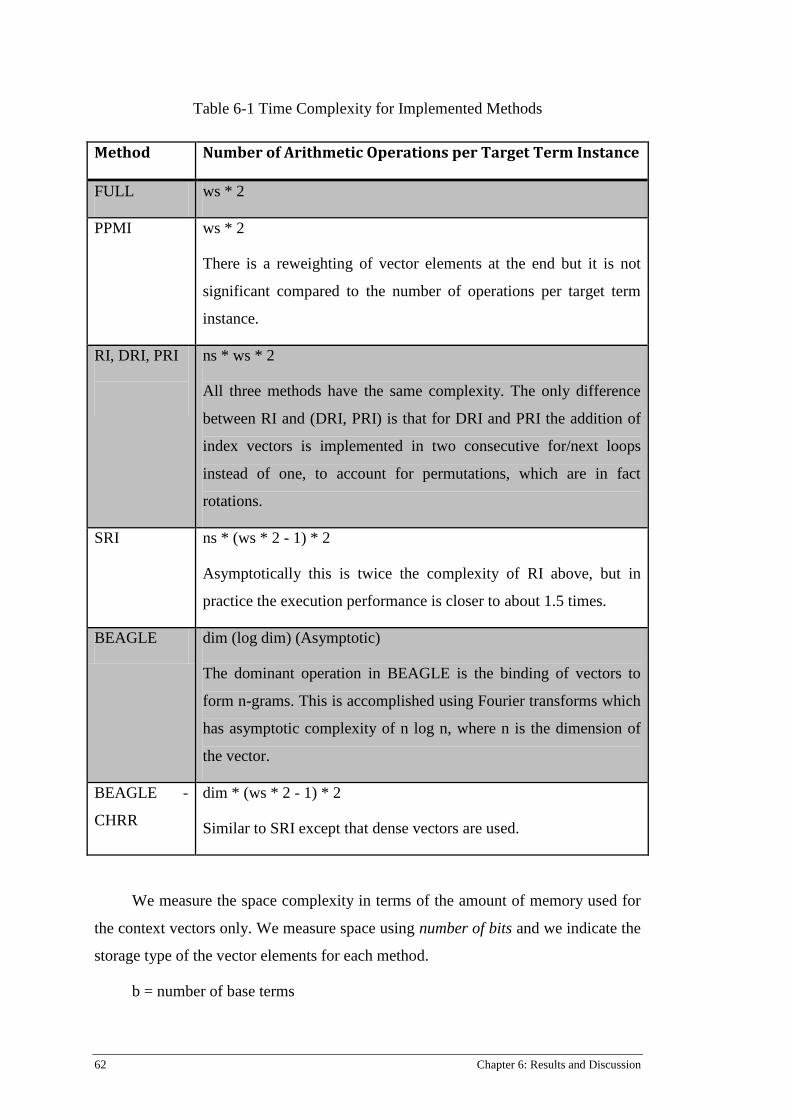
62 Chapter 6: Results and Discussion
Table 6-1 Time Complexity for Implemented Methods
Method Number of Arithmetic Operations per Target Term Instance
FULL ws * 2
PPMI ws * 2
There is a reweighting of vector elements at the end but it is not
significant compared to the number of operations per target term
instance.
RI, DRI, PRI
ns * ws * 2
All three methods have the same complexity. The only difference
between RI and (DRI, PRI) is that for DRI and PRI the addition of
index vectors is implemented in two consecutive for/next loops
instead of one, to account for permutations, which are in fact
rotations.
SRI ns * (ws * 2 - 1) * 2
Asymptotically this is twice the complexity of RI above, but in
practice the execution performance is closer to about 1.5 times.
BEAGLE dim (log dim) (Asymptotic)
The dominant operation in BEAGLE is the binding of vectors to
form n-grams. This is accomplished using Fourier transforms which
has asymptotic complexity of n log n, where n is the dimension of
the vector.
BEAGLE -
CHRR
dim * (ws * 2 - 1) * 2
Similar to SRI except that dense vectors are used.
We measure the space complexity in terms of the amount of memory used for
the context vectors only. We measure space using number of bits and we indicate the
storage type of the vector elements for each method.
b = number of base terms
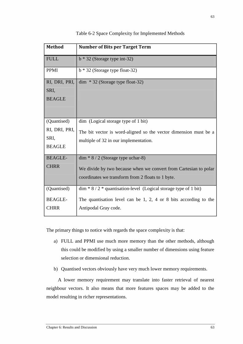
63
Chapter 6: Results and Discussion 63
Table 6-2 Space Complexity for Implemented Methods
Method Number of Bits per Target Term
FULL b * 32 (Storage type int-32)
PPMI b * 32 (Storage type float-32)
RI, DRI, PRI,
SRI,
BEAGLE
dim * 32 (Storage type float-32)
(Quantised)
RI, DRI, PRI,
SRI,
BEAGLE
dim (Logical storage type of 1 bit)
The bit vector is word-aligned so the vector dimension must be a
multiple of 32 in our implementation.
BEAGLE-
CHRR
dim * 8 / 2 (Storage type uchar-8)
We divide by two because when we convert from Cartesian to polar
coordinates we transform from 2 floats to 1 byte.
(Quantised)
BEAGLE-
CHRR
dim * 8 / 2 * quantisation-level (Logical storage type of 1 bit)
The quantisation level can be 1, 2, 4 or 8 bits according to the
Antipodal Gray code.
The primary things to notice with regards the space complexity is that:
a) FULL and PPMI use much more memory than the other methods, although
this could be modified by using a smaller number of dimensions using feature
selection or dimensional reduction.
b) Quantised vectors obviously have very much lower memory requirements.
A lower memory requirement may translate into faster retrieval of nearest
neighbour vectors. It also means that more features spaces may be added to the
model resulting in richer representations.
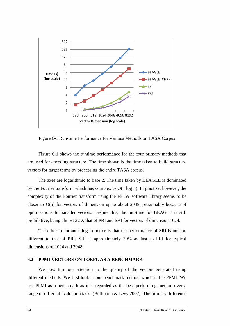
64 Chapter 6: Results and Discussion
Figure 6-1 Run-time Performance for Various Methods on TASA Corpus
Figure 6-1 shows the runtime performance for the four primary methods that
are used for encoding structure. The time shown is the time taken to build structure
vectors for target terms by processing the entire TASA corpus.
The axes are logarithmic to base 2. The time taken by BEAGLE is dominated
by the Fourier transform which has complexity O(n log n). In practise, however, the
complexity of the Fourier transform using the FFTW software library seems to be
closer to O(n) for vectors of dimension up to about 2048, presumably because of
optimisations for smaller vectors. Despite this, the run-time for BEAGLE is still
prohibitive, being almost 32 X that of PRI and SRI for vectors of dimension 1024.
The other important thing to notice is that the performance of SRI is not too
different to that of PRI. SRI is approximately 70% as fast as PRI for typical
dimensions of 1024 and 2048.
6.2 PPMI VECTORS ON TOEFL AS A BENCHMARK
We now turn our attention to the quality of the vectors generated using
different methods. We first look at our benchmark method which is the PPMI. We
use PPMI as a benchmark as it is regarded as the best performing method over a
range of different evaluation tasks (Bullinaria & Levy 2007). The primary difference
1
2
4
8
16
32
64
128
256
512
128 256 512 1024 2048 4096 8192
Time (s) (log scale)
Vector Dimension (log scale)
BEAGLE
BEAGLE_CHRR
SRI
PRI

65
Chapter 6: Results and Discussion 65
between PPMI and the random projection type methods that we have described
above, is that standard PPMI does not use any dimensional reduction, whereas the
random projection type methods, including RI, PRI, SRI and BEAGLE, do online
dimensional reduction. PPMI may use frequency thresholding of words, such that
words that occur very frequently or infrequently are removed. The random projection
methods are therefore useful in some contexts, such as when there are memory or
storage constraints, and PPMI vectors will be useful in other contexts, where such
constraints do not exist.
When encoding structure, e.g. n-grams, the number of possible features
explodes dramatically and it is not feasible to record statistics relating to all features.
In this instance random projection methods become very useful.
We use the PPMI benchmark as an indication of the best possible result that we
may expect from any method. We do not show results for the FULL method (full co-
occurrence vectors) as these vectors almost always give worse results than the PPMI
vectors. The PPMI vectors are the full vectors with PPMI weighting applied to the
elements.
Figure 6-2 PPMI Vectors on TOEFL Test
Our results support the findings of Bullinaria and Levy (2007) regarding the
performance of PPMI vectors on TOEFL. We obtained a score of 87.5% using PPMI
vectors with the INEX corpus and using vector dimensions of approximately 28 000.
0
10
20
30
40
50
60
70
80
90
100
TOEFL Score (%)
PPMI Vectors
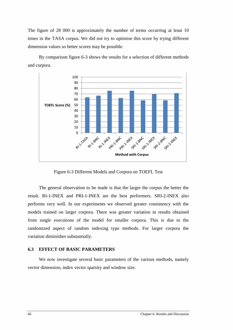
66 Chapter 6: Results and Discussion
The figure of 28 000 is approximately the number of terms occurring at least 10
times in the TASA corpus. We did not try to optimise this score by trying different
dimension values so better scores may be possible.
By comparison figure 6-3 shows the results for a selection of different methods
and corpora.
Figure 6-3 Different Models and Corpora on TOEFL Test
The general observation to be made is that the larger the corpus the better the
result. RI-1-INEX and PRI-1-INEX are the best performers. SRI-2-INEX also
performs very well. In our experiments we observed greater consistency with the
models trained on larger corpora. There was greater variation in results obtained
from single executions of the model for smaller corpora. This is due to the
randomized aspect of random indexing type methods. For larger corpora the
variation diminishes substantially.
6.3 EFFECT OF BASIC PARAMETERS
We now investigate several basic parameters of the various methods, namely
vector dimension, index vector sparsity and window size.
0
10
20
30
40
50
60
70
80
90
100
TOEFL Score (%)
Method with Corpus

67
Chapter 6: Results and Discussion 67
6.3.1 Effect of Vector Dimension
As expected the performance on the TOEFL test increases as we increase the
vector dimension. We decided to use a dimension of 1024 for the remaining
experiments.
Figure 6-4 Effect of Vector Dimension of TOEFL Test
6.3.2 Effect of Sparsity
We chose several different Random Indexing type methods to evaluate the
effect of sparsity on performance with the TOEFL test. The window radius for each
method was kept at 1. The vector dimension was 1024 and log entropy weighting
was used.
30
35
40
45
50
55
60
65
70
75
80
64 128 256 512 1024 2048 4096 8192
TOEFL Score (%)
Context Vector Dimension
RI-TASA
PRI-TASA
SRI-TASA
BEAGLE-TASA
RI-BNC

68 Chapter 6: Results and Discussion
Figure 6-5 Selection of Models with Vectors of Various Sparsity Levels
The primary finding of this experiment is that performance as measured on the
TOEFL task is a little erratic in terms of the number of seeds that are used. On the
other hand it also shows that using fewer seeds (more sparse index vectors) does not
give predictably worse performance, contrary to what one may expect. This is an
interesting result in that more sparse index vectors gives faster run times.
In the rest of the experiments we use 32 seeds with a vector dimension of 1024.
6.3.3 Effect of Window Size
As has been reported in most published work a small window size is best for
Random Indexing methods. We confirm Sahlgren (2006) that a window radius size
of 1 is best. The BEAGLE type methods on the other hand seem to perform better
with larger window sizes. We consistently found that SRI is best with a window size
of 2, which is equivalent to encoding the n-grams A-B, B-C, C-D in the context “A B
_ C D” where “_” indicates the target word.
B-CHRR-4 refers to BEAGLE-CHRR quantised using 4 bits per phase angle.
45
50
55
60
65
70
75
8 32 56 80 104 128 152 176 200
TOEFL Score (%)
Number of Seeds
RI-TASA
PRI-TASA
RI-BNC
PRI-BNC
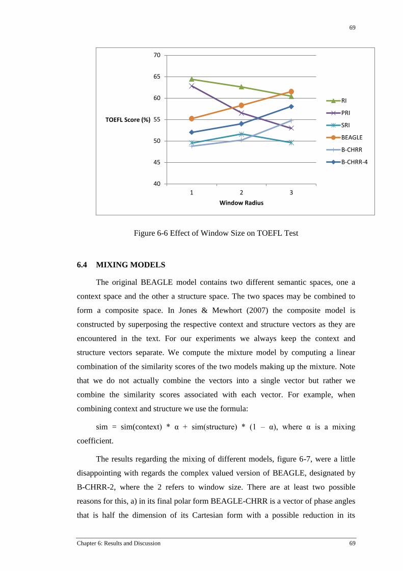
69
Chapter 6: Results and Discussion 69
Figure 6-6 Effect of Window Size on TOEFL Test
6.4 MIXING MODELS
The original BEAGLE model contains two different semantic spaces, one a
context space and the other a structure space. The two spaces may be combined to
form a composite space. In Jones & Mewhort (2007) the composite model is
constructed by superposing the respective context and structure vectors as they are
encountered in the text. For our experiments we always keep the context and
structure vectors separate. We compute the mixture model by computing a linear
combination of the similarity scores of the two models making up the mixture. Note
that we do not actually combine the vectors into a single vector but rather we
combine the similarity scores associated with each vector. For example, when
combining context and structure we use the formula:
sim = sim(context) * α + sim(structure) * (1 – α), where α is a mixing
coefficient.
The results regarding the mixing of different models, figure 6-7, were a little
disappointing with regards the complex valued version of BEAGLE, designated by
B-CHRR-2, where the 2 refers to window size. There are at least two possible
reasons for this, a) in its final polar form BEAGLE-CHRR is a vector of phase angles
that is half the dimension of its Cartesian form with a possible reduction in its
40
45
50
55
60
65
70
1 2 3
TOEFL Score (%)
Window Radius
RI
PRI
SRI
BEAGLE
B-CHRR
B-CHRR-4
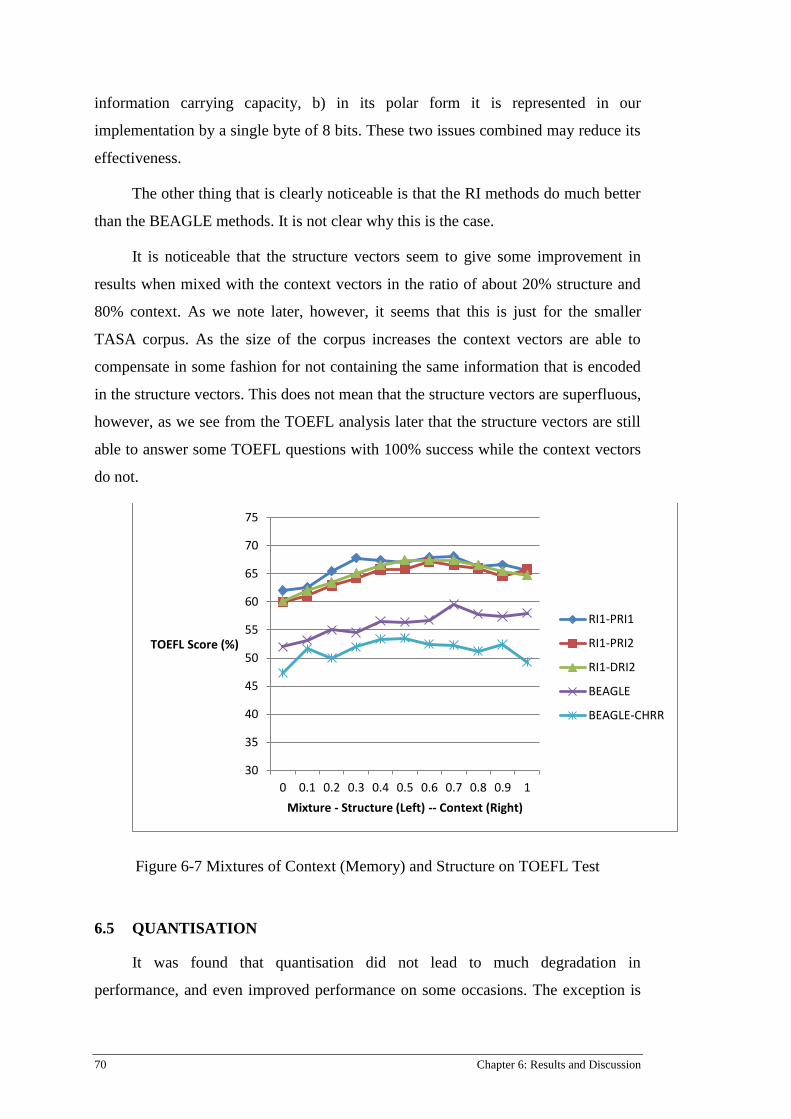
70 Chapter 6: Results and Discussion
information carrying capacity, b) in its polar form it is represented in our
implementation by a single byte of 8 bits. These two issues combined may reduce its
effectiveness.
The other thing that is clearly noticeable is that the RI methods do much better
than the BEAGLE methods. It is not clear why this is the case.
It is noticeable that the structure vectors seem to give some improvement in
results when mixed with the context vectors in the ratio of about 20% structure and
80% context. As we note later, however, it seems that this is just for the smaller
TASA corpus. As the size of the corpus increases the context vectors are able to
compensate in some fashion for not containing the same information that is encoded
in the structure vectors. This does not mean that the structure vectors are superfluous,
however, as we see from the TOEFL analysis later that the structure vectors are still
able to answer some TOEFL questions with 100% success while the context vectors
do not.
Figure 6-7 Mixtures of Context (Memory) and Structure on TOEFL Test
6.5 QUANTISATION
It was found that quantisation did not lead to much degradation in
performance, and even improved performance on some occasions. The exception is
30
35
40
45
50
55
60
65
70
75
0 0.1 0.2 0.3 0.4 0.5 0.6 0.7 0.8 0.9 1
TOEFL Score (%)
Mixture - Structure (Left) -- Context (Right)
RI1-PRI1
RI1-PRI2
RI1-DRI2
BEAGLE
BEAGLE-CHRR
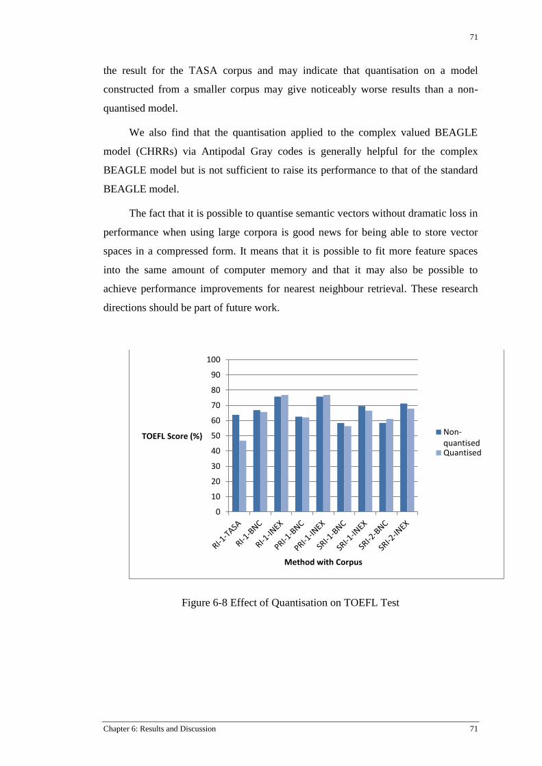
71
Chapter 6: Results and Discussion 71
the result for the TASA corpus and may indicate that quantisation on a model
constructed from a smaller corpus may give noticeably worse results than a non-
quantised model.
We also find that the quantisation applied to the complex valued BEAGLE
model (CHRRs) via Antipodal Gray codes is generally helpful for the complex
BEAGLE model but is not sufficient to raise its performance to that of the standard
BEAGLE model.
The fact that it is possible to quantise semantic vectors without dramatic loss in
performance when using large corpora is good news for being able to store vector
spaces in a compressed form. It means that it is possible to fit more feature spaces
into the same amount of computer memory and that it may also be possible to
achieve performance improvements for nearest neighbour retrieval. These research
directions should be part of future work.
Figure 6-8 Effect of Quantisation on TOEFL Test
0
10
20
30
40
50
60
70
80
90
100
TOEFL Score (%)
Method with Corpus
Non-quantisedQuantised

72 Chapter 6: Results and Discussion
Figure 6-9 Effect of Quantisation Levels on TOEFL Test
6.6 PERFORMANCE ON WS353
As noted previously in the description for this task (5.1.2), success on this task
seems to be determined to some extent by how terms are clustered in the space.
Cosine similarity gives an indication of semantic relatedness in the vicinity of a
target term but is not an absolute measure of semantic relatedness for the whole
space. A different similarity metric that could somehow capture the ranking of
semantic relatedness at a global level is sure to perform better on this task. Various
ideas suggest themselves but are outside the scope of this thesis.
PPMI vectors are clearly best on WS353 and DRI-2-INEX performs
surprisingly well. The methods which incorporate purely structural information were
found to perform very poorly. Something that is not shown in Figure 6-10 is the
effect of quantisation. This was found to always give a slight improvement in
performance.
From the results it seems that very specific structural information, such as that
captured by SRI, does not help greatly in this task, while a small amount of more
general structural information, such as that is captured by DRI, does help quite a lot.
48
50
52
54
56
58
60
62
64
Q0 Q1 Q2 Q4 Q8
TOEFL Score (%)
Quantisation Levels
BEAGLE-3
BEAGLE-CHRR-3

73
Chapter 6: Results and Discussion 73
Figure 6-10 A Selection of Methods and Scores on WS353
6.7 SEMANTIC SPACE OVERLAP
The Semantic Space Overlap task is basically an attempt to discover how much
information is shared between two different spaces. As described in chapter 5 we use
the 50 nearest neighbours as the neighbourhood of a target word and we sample 1000
random words to compute the overlap of two semantic spaces. The results reported
below in Table 6-3 are from the TASA corpus. “B_C-1” and “B_S-1” indicate
BEAGLE context vectors and BEAGLE structure vectors respectively, with a
window radius of one. “BC_C-1” and “BC_S-1” indicate BEAGLE-CHRR context
vectors and BEAGLE-CHRR structure vectors respectively, with a window radius of
one.
Table 6-3 Semantic Space Overlap
RI-1 RI-2 PRI-1 SRI-1 B_C-1 B_S-1 BC_C-1 BC_S-1
RI-1 54% 28% 22% 4% 24% 3% 14% 3%
RI-2 30% 42% 25% 4% 14% 3% 11% 3%
PRI-1 22% 25% 30% 4% 15% 3% 12% 3%
SRI-1 4% 4% 4% 50% 4% 41% 4% 31%
B_C-1 23% 14% 16% 5% 63% 4% 24% 3%
B_S-1 4% 3% 4% 43% 4% 48% 3% 28%
BC_C-1 14% 11% 11% 3% 23% 3% 24% 2%
BC_S-1 3% 2% 2% 33% 3% 29% 2% 26%
0
0.1
0.2
0.3
0.4
0.5
0.6
WS353 Score (cor.)
Method and Corpus

74 Chapter 6: Results and Discussion
We generate two separate models for each method. One model is associated
with the columns and the other with the rows.
The first thing that one notices is that the greatest degrees of overlap occur
when a model of the same type is tested for overlap with another model of the same
type, as we might expect. By “type” we mean the same method and same parameters.
It might be a little surprising, however, to see that the greatest degree of overlap is
63% which occurs for BEAGLE context vectors. It indicates that there is a fair
degree of variability in the spaces constructed using randomised methods such as
BEAGLE and Random Indexing, at least when constructed from the TASA corpus.
It is interesting that SRI shows greater overlap with BEAGLE structure vectors
than the BEAGLE-CHRR structure vectors.
The overlap of 28/30% for RI-1 and RI-2 is surprising in that changing the
window radius by one makes such a large difference, as compared to 54% for RI-1
and RI-1.
A good result from this test is that the overlap for SRI-1 and B_S-1 is 43% as
compared to 48% for B_S-1 and B_S-1. It indicates a very large degree of overlap
between the space created by the BEAGLE structure vectors and the space created by
SRI. This is a good result as the intention had been to find a more efficient method
for encoding the information contained in BEAGLE structure vectors, which we
have done with SRI.
6.8 TOEFL ANALYSIS
Many studies have used the TOEFL test as a way of assessing the quality of
semantic relatedness models. One thing that would be useful, however, in better
understanding the difference between models, is to analyse what TOEFL questions
different models have difficulty with. To this end we have collected statistics from
many TOEFL evaluations and have chosen a subset of questions that, from manual
inspection, seem to be good differentiators of performance by different models. The
statistics are interesting in that they cast some light on the differences between
models.
In Table 6-4 we show the performance of 7 different models. These results are
based on models trained using TASA. Table 6-5 includes the performance of some

75
Chapter 6: Results and Discussion 75
models from Table 6-4, for comparison purposes, also trained on TASA, but
augments these with results for BEAGLE context and structure methods.
Table 6-4 Analysis of TOEFL Results for Different Methods and TASA Corpus
Qs RI-1 RI-2 RI-3 PRI-1 PRI-2 SRI-1 SRI-2
1 10 15 25 35 25 0 0
2 20 30 35 25 30 15 25
3 100 100 90 75 40 60 100
4 0 75 45 60 50 15 0
7 100 85 5 45 55 35 0
9 35 15 100 30 20 0 0
15 30 35 35 50 30 15 100
16 0 0 5 50 15 100 100
17 45 35 40 70 50 5 90
18 75 95 80 85 75 0 0
24 15 10 30 15 35 100 65
25 0 0 25 20 15 70 95
35 25 75 35 10 15 15 55
38 35 25 15 40 50 45 60
41 100 100 100 100 100 95 0
46 95 100 100 95 70 70 100
54 15 0 15 10 20 0 0
67 55 45 60 30 40 0 15
72 0 10 0 15 10 75 0
78 15 5 40 10 25 100 100
The percentage of times that a model answered the given question correctly is
indicated in the corresponding cell. So, for example, RI answered correctly only 20%
of the time for question 2, whereas RI-2 answered 85% of the time for question 7.
We have used the arbitrary figures of 25% and 75% as cut off values to assign
colours to the extreme counts - the colour “red” to poor results and the colour
“green” to good results. Note also that the numbering of questions starts at 0.
Question 0, however, is not part of the selected subset of questions.
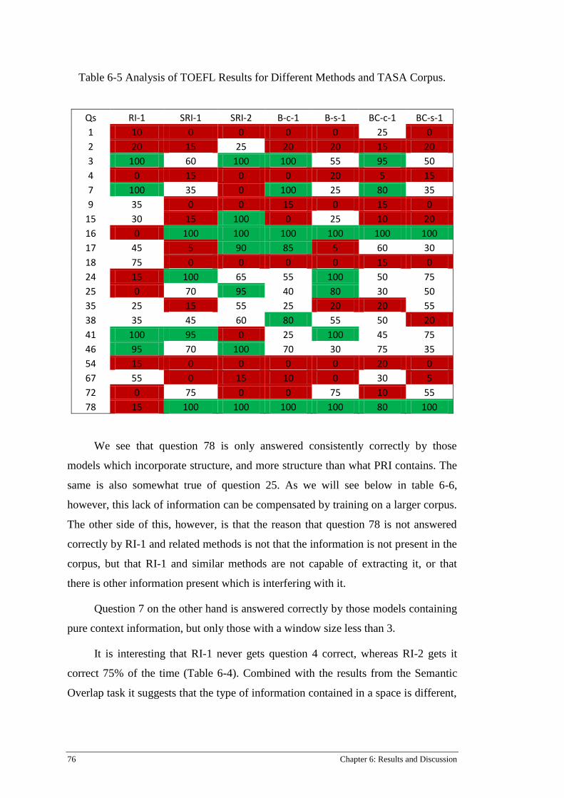
76 Chapter 6: Results and Discussion
Table 6-5 Analysis of TOEFL Results for Different Methods and TASA Corpus.
Qs RI-1 SRI-1 SRI-2 B-c-1 B-s-1 BC-c-1 BC-s-1
1 10 0 0 0 0 25 0
2 20 15 25 20 20 15 20
3 100 60 100 100 55 95 50
4 0 15 0 0 20 5 15
7 100 35 0 100 25 80 35
9 35 0 0 15 0 15 0
15 30 15 100 0 25 10 20
16 0 100 100 100 100 100 100
17 45 5 90 85 5 60 30
18 75 0 0 0 0 15 0
24 15 100 65 55 100 50 75
25 0 70 95 40 80 30 50
35 25 15 55 25 20 20 55
38 35 45 60 80 55 50 20
41 100 95 0 25 100 45 75
46 95 70 100 70 30 75 35
54 15 0 0 0 0 20 0
67 55 0 15 10 0 30 5
72 0 75 0 0 75 10 55
78 15 100 100 100 100 80 100
We see that question 78 is only answered consistently correctly by those
models which incorporate structure, and more structure than what PRI contains. The
same is also somewhat true of question 25. As we will see below in table 6-6,
however, this lack of information can be compensated by training on a larger corpus.
The other side of this, however, is that the reason that question 78 is not answered
correctly by RI-1 and related methods is not that the information is not present in the
corpus, but that RI-1 and similar methods are not capable of extracting it, or that
there is other information present which is interfering with it.
Question 7 on the other hand is answered correctly by those models containing
pure context information, but only those with a window size less than 3.
It is interesting that RI-1 never gets question 4 correct, whereas RI-2 gets it
correct 75% of the time (Table 6-4). Combined with the results from the Semantic
Overlap task it suggests that the type of information contained in a space is different,

77
Chapter 6: Results and Discussion 77
even when comparing models that only differ by 1 in the size of the context window
used to generate them.
Table 6-5 supports the results of Table 6-4 with regard to question 25 but not
with regards to question 78, in that BEAGLE context vectors are able to answer
correctly where RI context vectors were not.
Table 6-6 Analysis of TOEFL Results for Different Methods and Different Corpora
Qs RI-1-TASA
RI-1-BNC
RI-1-INEX
PRI-1-BNC
PRI-1-INEX
SRI-1-BNC
SRI-1-INEX
SRI-2-BNC
SRI-2-INEX
1 10 0 100 0 100 0 100 0 100
2 20 100 90 30 70 20 20 60 70
3 100 90 0 60 0 100 10 100 80
4 0 100 50 100 100 100 100 100 100
7 100 10 100 10 100 0 100 0 100
9 35 100 100 60 100 50 100 60 100
15 30 0 100 10 100 100 100 100 100
16 0 100 100 100 100 100 100 100 100
17 45 0 10 10 5 30 100 100 100
18 75 0 0 30 0 0 0 0 0
24 15 90 100 80 100 20 90 30 100
25 0 90 100 100 100 10 0 0 0
35 25 0 100 0 100 0 100 0 100
38 35 0 60 0 45 50 60 40 90
41 100 20 100 0 100 40 100 0 100
46 95 0 50 0 0 0 10 0 0
54 15 80 90 20 50 100 100 100 100
67 55 100 100 100 95 0 0 0 0
72 0 10 0 10 0 0 0 0 0
78 15 90 100 90 100 100 100 100 100
63.81 66.86 75.75 62.63 75.75 58.38 69.63 58.5 71.25
In Table 6-6 it is interesting that RI-1 trained on TASA answers question 46
correctly 95% of the time while all other methods, except RI-1 trained on INEX, fail.
The above TOEFL analysis is a first step in a more in depth analysis of
performance on the TOEFL test by different models. Future work should include an
investigation of what sorts of questions each model performs well on and should also
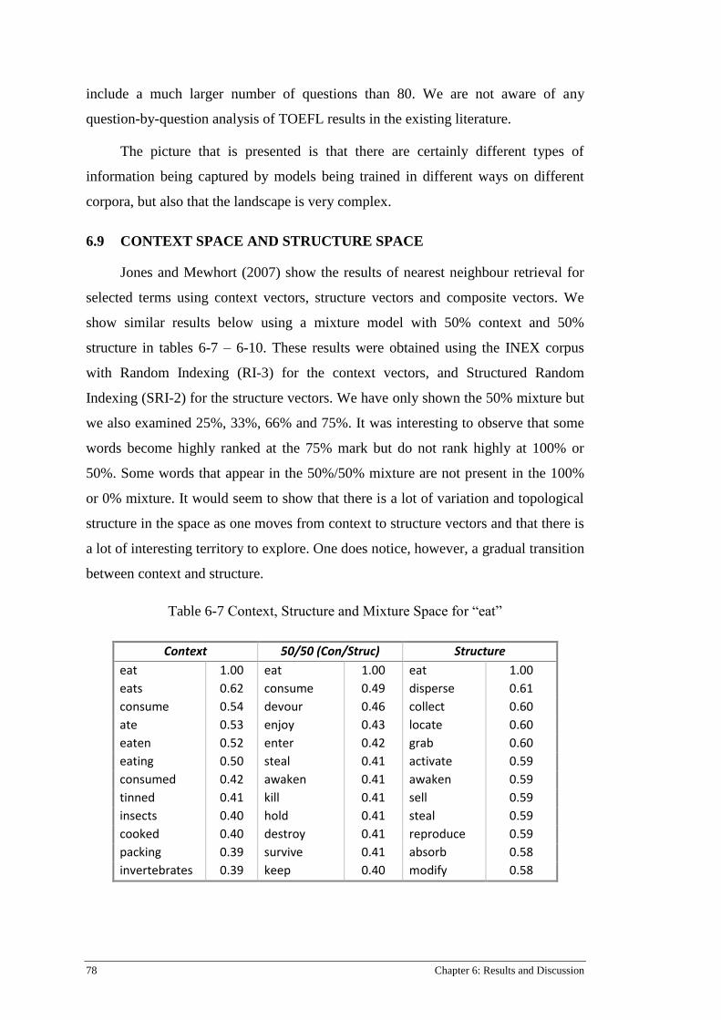
78 Chapter 6: Results and Discussion
include a much larger number of questions than 80. We are not aware of any
question-by-question analysis of TOEFL results in the existing literature.
The picture that is presented is that there are certainly different types of
information being captured by models being trained in different ways on different
corpora, but also that the landscape is very complex.
6.9 CONTEXT SPACE AND STRUCTURE SPACE
Jones and Mewhort (2007) show the results of nearest neighbour retrieval for
selected terms using context vectors, structure vectors and composite vectors. We
show similar results below using a mixture model with 50% context and 50%
structure in tables 6-7 – 6-10. These results were obtained using the INEX corpus
with Random Indexing (RI-3) for the context vectors, and Structured Random
Indexing (SRI-2) for the structure vectors. We have only shown the 50% mixture but
we also examined 25%, 33%, 66% and 75%. It was interesting to observe that some
words become highly ranked at the 75% mark but do not rank highly at 100% or
50%. Some words that appear in the 50%/50% mixture are not present in the 100%
or 0% mixture. It would seem to show that there is a lot of variation and topological
structure in the space as one moves from context to structure vectors and that there is
a lot of interesting territory to explore. One does notice, however, a gradual transition
between context and structure.
Table 6-7 Context, Structure and Mixture Space for “eat”
Context 50/50 (Con/Struc) Structure
eat 1.00 eat 1.00 eat 1.00
eats 0.62 consume 0.49 disperse 0.61
consume 0.54 devour 0.46 collect 0.60
ate 0.53 enjoy 0.43 locate 0.60
eaten 0.52 enter 0.42 grab 0.60
eating 0.50 steal 0.41 activate 0.59
consumed 0.42 awaken 0.41 awaken 0.59
tinned 0.41 kill 0.41 sell 0.59
insects 0.40 hold 0.41 steal 0.59
cooked 0.40 destroy 0.41 reproduce 0.59
packing 0.39 survive 0.41 absorb 0.58
invertebrates 0.39 keep 0.40 modify 0.58
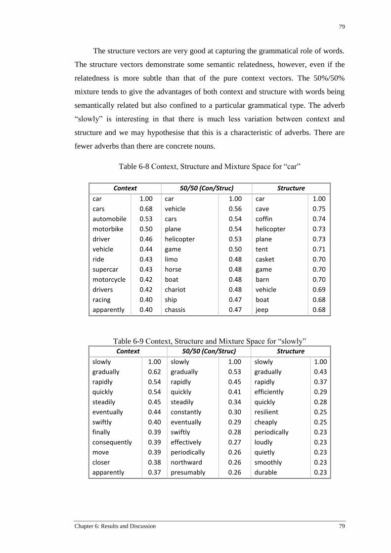
79
Chapter 6: Results and Discussion 79
The structure vectors are very good at capturing the grammatical role of words.
The structure vectors demonstrate some semantic relatedness, however, even if the
relatedness is more subtle than that of the pure context vectors. The 50%/50%
mixture tends to give the advantages of both context and structure with words being
semantically related but also confined to a particular grammatical type. The adverb
“slowly” is interesting in that there is much less variation between context and
structure and we may hypothesise that this is a characteristic of adverbs. There are
fewer adverbs than there are concrete nouns.
Table 6-8 Context, Structure and Mixture Space for “car”
Context 50/50 (Con/Struc) Structure
car 1.00 car 1.00 car 1.00
cars 0.68 vehicle 0.56 cave 0.75
automobile 0.53 cars 0.54 coffin 0.74
motorbike 0.50 plane 0.54 helicopter 0.73
driver 0.46 helicopter 0.53 plane 0.73
vehicle 0.44 game 0.50 tent 0.71
ride 0.43 limo 0.48 casket 0.70
supercar 0.43 horse 0.48 game 0.70
motorcycle 0.42 boat 0.48 barn 0.70
drivers 0.42 chariot 0.48 vehicle 0.69
racing 0.40 ship 0.47 boat 0.68
apparently 0.40 chassis 0.47 jeep 0.68
Table 6-9 Context, Structure and Mixture Space for “slowly”
Context 50/50 (Con/Struc) Structure
slowly 1.00 slowly 1.00 slowly 1.00
gradually 0.62 gradually 0.53 gradually 0.43
rapidly 0.54 rapidly 0.45 rapidly 0.37
quickly 0.54 quickly 0.41 efficiently 0.29
steadily 0.45 steadily 0.34 quickly 0.28
eventually 0.44 constantly 0.30 resilient 0.25
swiftly 0.40 eventually 0.29 cheaply 0.25
finally 0.39 swiftly 0.28 periodically 0.23
consequently 0.39 effectively 0.27 loudly 0.23
move 0.39 periodically 0.26 quietly 0.23
closer 0.38 northward 0.26 smoothly 0.23
apparently 0.37 presumably 0.26 durable 0.23
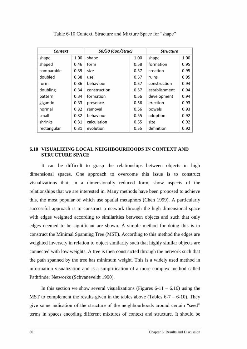
80 Chapter 6: Results and Discussion
Table 6-10 Context, Structure and Mixture Space for “shape”
Context 50/50 (Con/Struc) Structure
shape 1.00 shape 1.00 shape 1.00
shaped 0.46 form 0.58 formation 0.95
comparable 0.39 size 0.57 creation 0.95
doubled 0.38 use 0.57 ruins 0.95
form 0.36 behaviour 0.57 construction 0.94
doubling 0.34 construction 0.57 establishment 0.94
pattern 0.34 formation 0.56 development 0.94
gigantic 0.33 presence 0.56 erection 0.93
normal 0.32 removal 0.56 bowels 0.93
small 0.32 behaviour 0.55 adoption 0.92
shrinks 0.31 calculation 0.55 size 0.92
rectangular 0.31 evolution 0.55 definition 0.92
6.10 VISUALIZING LOCAL NEIGHBOURHOODS IN CONTEXT AND
STRUCTURE SPACE
It can be difficult to grasp the relationships between objects in high
dimensional spaces. One approach to overcome this issue is to construct
visualizations that, in a dimensionally reduced form, show aspects of the
relationships that we are interested in. Many methods have been proposed to achieve
this, the most popular of which use spatial metaphors (Chen 1999). A particularly
successful approach is to construct a network through the high dimensional space
with edges weighted according to similarities between objects and such that only
edges deemed to be significant are shown. A simple method for doing this is to
construct the Minimal Spanning Tree (MST). According to this method the edges are
weighted inversely in relation to object similarity such that highly similar objects are
connected with low weights. A tree is then constructed through the network such that
the path spanned by the tree has minimum weight. This is a widely used method in
information visualization and is a simplification of a more complex method called
Pathfinder Networks (Schvaneveldt 1990).
In this section we show several visualizations (Figures 6-11 – 6.16) using the
MST to complement the results given in the tables above (Tables 6-7 – 6-10). They
give some indication of the structure of the neighbourhoods around certain “seed”
terms in spaces encoding different mixtures of context and structure. It should be
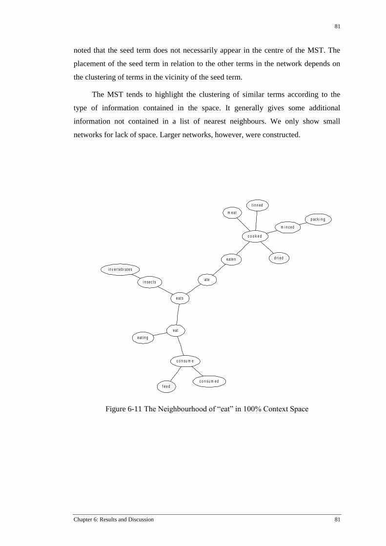
81
Chapter 6: Results and Discussion 81
noted that the seed term does not necessarily appear in the centre of the MST. The
placement of the seed term in relation to the other terms in the network depends on
the clustering of terms in the vicinity of the seed term.
The MST tends to highlight the clustering of similar terms according to the
type of information contained in the space. It generally gives some additional
information not contained in a list of nearest neighbours. We only show small
networks for lack of space. Larger networks, however, were constructed.
Figure 6-11 The Neighbourhood of “eat” in 100% Context Space
e a t
e a t s
c o n su m e
e at i n g
i n v e r t e b r a t e s
i n se c t sa t e
c o n s u m e df e e d
t i n n ed
c o o k e d
e a t e n d r i e d
m i n c e d
m e a t
p a c k i n g

82 Chapter 6: Results and Discussion
Figure 6-12 The Neighbourhood of “eat” in 50% Context / 50% Structure Space
Figure 6-13 The Neighbourhood of “eat” in 100% Structure Space
s u r v i v e
e n t e r
d e s t r o y
h o l d
e n j o y
o b s e r v e
c o l l e c t
e a t
c o n s u m e
d e v o u r
s t e a l
a w a k e n
k e e p
a c t i v a t e
k i l l
s e l l
s e l l s t e a l
e a t
d i s p e r s e
c o l l e c t
l o c a t e
a w a k e n
t e a c h
a c t i v a t e
r e p r o d u c e
i n t e r c e p t
d i s a r m
g r a b
m o d i f y
e n j o y
a b s o r b
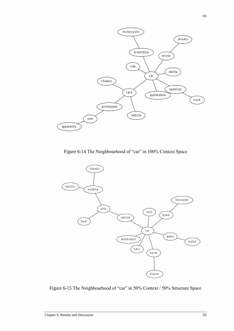
83
Chapter 6: Results and Discussion 83
Figure 6-14 The Neighbourhood of “car” in 100% Context Space
Figure 6-15 The Neighbourhood of “car” in 50% Context / 50% Structure Space
c ar
su p erc arc ar s
autom obi l e
m o to rb i k e
r i de
raci ng
dr i v er
t ruck
v ehi cl e
ch assi s
p ro to ty p es
m o to rcy c l e
o n e
apparentl y
dr i v ers
h e l i c o p t e r
p l an e
c a r
g am e
v eh i c l e
c a r s
h o r se
l i m o
au t o m o b i l e
b o a t
s h i p
c h a s s i s
b u i l d i n g
m a t c h
c h a r i o t
f a c t o r y

84 Chapter 6: Results and Discussion
Figure 6-16 The Neighbourhood of “car” in 100% Structure Space
Once we move to the 100% structure space the semantic relations between the
terms becomes less clear, but not altogether missing, and the shared grammatical
function of the terms becomes very clear.
6.11 STRUCTURE QUERIES USING QUANTISED STRUCTURED
RANDOM INDEXING
Jones and Mewhort (2007), and subsequent related publications, show
examples of models applied to phrase completion tasks demonstrating the ability of
the model to fill in the blanks of various phrases. In the same spirit we present some
exemplary results here using quantised SRI. Because we are using the quantised form
of SRI the similarities are returned as “number of bits”. In the tables below we show
the similarity in number of bits out of a total possible 64 bits. All results were
obtained using the BNC with a vector dimension of 4096 and sparse index vectors of
length 64. SRI-2 was used which means that for each target word we record the
bigrams to the left, centre and right of the target word.
p l an ec av e
h el i co p ter
c ar
j eep
b ar n
c o f f i n
t en t
g am ec ask et
d o c u m en t
tu r r et
sh i p
b o at
v eh i c l e
b ar rel
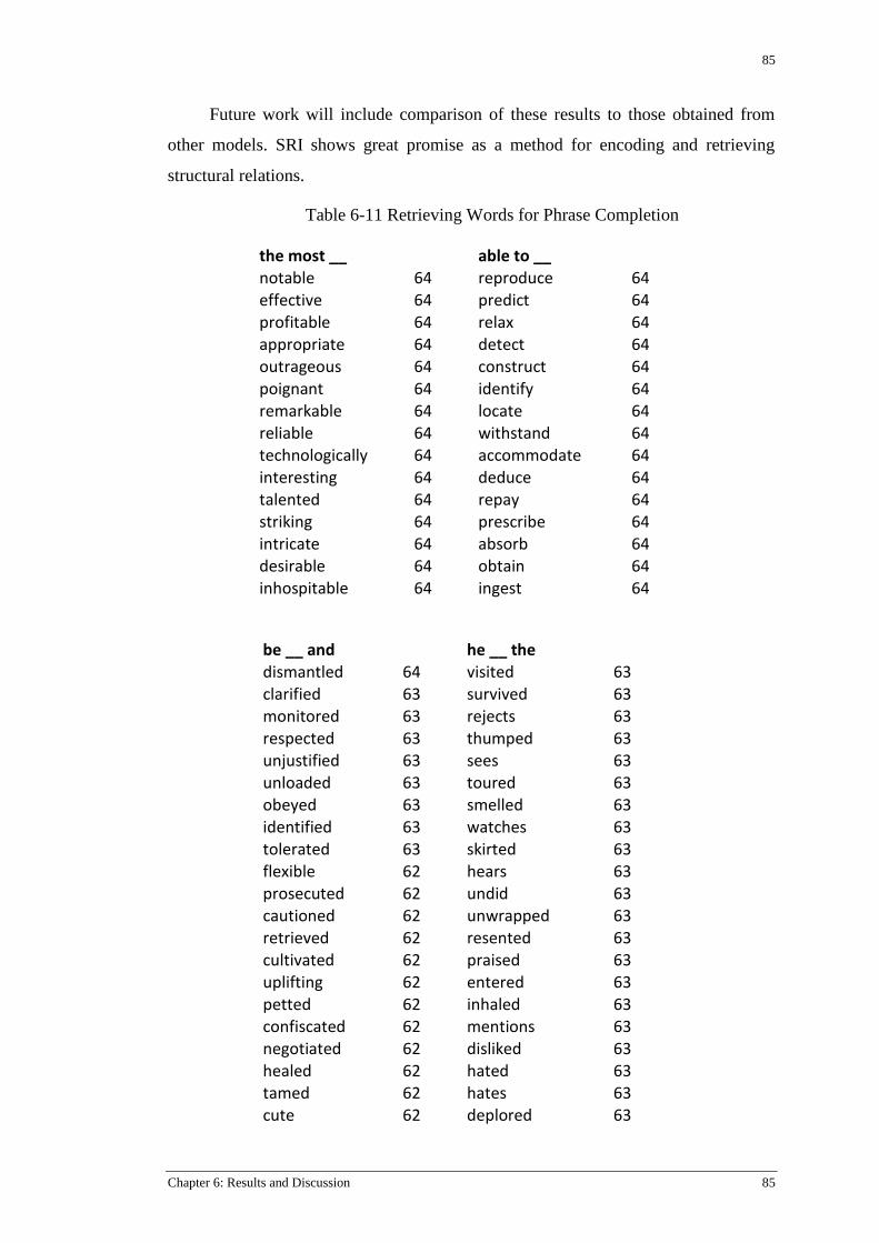
85
Chapter 6: Results and Discussion 85
Future work will include comparison of these results to those obtained from
other models. SRI shows great promise as a method for encoding and retrieving
structural relations.
Table 6-11 Retrieving Words for Phrase Completion
the most __
able to __ notable 64 reproduce 64
effective 64 predict 64 profitable 64 relax 64 appropriate 64 detect 64 outrageous 64 construct 64
poignant 64 identify 64 remarkable 64 locate 64 reliable 64 withstand 64 technologically 64 accommodate 64 interesting 64 deduce 64 talented 64 repay 64 striking 64 prescribe 64 intricate 64 absorb 64 desirable 64 obtain 64 inhospitable 64 ingest 64
be __ and
he __ the dismantled 64 visited 63
clarified 63 survived 63 monitored 63 rejects 63 respected 63 thumped 63 unjustified 63 sees 63 unloaded 63 toured 63 obeyed 63 smelled 63 identified 63 watches 63 tolerated 63 skirted 63 flexible 62 hears 63
prosecuted 62 undid 63 cautioned 62 unwrapped 63 retrieved 62 resented 63 cultivated 62 praised 63 uplifting 62 entered 63 petted 62 inhaled 63 confiscated 62 mentions 63 negotiated 62 disliked 63 healed 62 hated 63 tamed 62 hates 63 cute 62 deplored 63
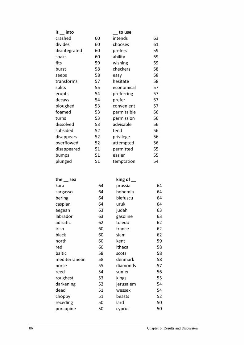
86 Chapter 6: Results and Discussion
it __ into
__ to use crashed 60 intends 63
divides 60 chooses 61 disintegrated 60 prefers 59 soaks 60 ability 59 fits 59 wishing 59 burst 58 checkers 58 seeps 58 easy 58 transforms 57 hesitate 58 splits 55 economical 57 erupts 54 preferring 57 decays 54 prefer 57
ploughed 53 convenient 57 foamed 53 permissible 56 turns 53 permission 56 dissolved 53 advisable 56 subsided 52 tend 56 disappears 52 privilege 56 overflowed 52 attempted 56 disappeared 51 permitted 55 bumps 51 easier 55 plunged 51 temptation 54
the __ sea
king of __ kara 64 prussia 64
sargasso 64 bohemia 64 bering 64 blefuscu 64 caspian 64 uruk 64 aegean 63 judah 63 labrador 63 gasoline 63 adriatic 62 toledo 62 irish 60 france 62 black 60 siam 62 north 60 kent 59
red 60 ithaca 58 baltic 58 scots 58 mediterranean 58 denmark 58 norse 55 diamonds 57 reed 54 sumer 56 roughest 53 kings 55 darkening 52 jerusalem 54 dead 51 wessex 54 choppy 51 beasts 52 receding 50 lard 50 porcupine 50 cyprus 50
87
Chapter 6: Results and Discussion 87
6.12 GENERAL DISCUSSION
We now move onto some general discussion regarding the contributions of this
thesis and the experimental results.
One of the points that this research has highlighted is the difficulty in assessing
the relative merits of different semantic models. Different models can contain
different types of information even when constructed using the same underlying
method but with a single parameter perturbation.
For small to medium sized corpora (TASA), structure information seems to
help on the TOEFL evaluation task, with the correct mix of context and structure.
For larger corpora (BNC, INEX) the contribution of structure as providing something
that non-structure does not, is less clear, at least for the TOEFL test. It would be
useful to have a larger TOEFL test. From the results one has the feeling that there are
sharp transitions in the space of the terms appearing in the TOEFL test such that a
model may flip from being correct to incorrect with a small adjustment, at least when
trained on smaller corpora such as TASA. The results tend to be more robust with
larger corpora.
6.12.1 The Semantic Space Continuum
Amongst the different methods we can identify the following spectrum in
terms of contribution of specific structure:
1) RI and BEAGLE Context : no structure, only context
2) DRI: structure in terms of before and after target word
3) PRI: structure in terms of words being bound to positions relative to the
target term.
4) SRI and BEAGLE Structure: n-grams encoded and positioned relative to
the target term.
As pointed out by Sahlgren (2006) when referring to the difference between
syntagmatic and paradigmatic word spaces, “the difference between word spaces
produced with different types of contexts is more like a semantic continuum, where
syntagmatic and paradigmatic relations represent the extremities.” We have found
throughout our experiments that the same can be said for the difference between
context/memory vectors and structure vectors. Structure vectors clearly have a
88 Chapter 6: Results and Discussion
tendency to cluster words that have the same grammatical role. The structure vectors
still retain some semantic relatedness, however. Occasionally it was noticed that the
neighbourhoods of pure context vectors encoded information that one would usually
associate with structure vectors, such as clustering people’s proper names. The
degree of variation between context and structure vectors is dependent on the
grammatical role of the target term. It was found that the nearest neighbours of
adverbs did not vary greatly between context and structure.
A semantic continuum can definitely be observed when moving between
context and structure. Besides the few observations that we have made here, a more
detailed analysis is required to identify the general patterns in the different spaces for
different words.
There is clearly a need for methods to be able to identify, characterise and
quantify the contribution of different semantic spaces. The information captured by
RI-1 is different to that of RI-2, and likewise for SRI-1 and SRI-2. Although we have
not addressed it in this thesis, the information captured by different methods also
depends on the base (index) terms used as features. For example, if one was to only
use prepositions and postpositions as features, very different information would be
captured compared to using all grammatical types.
6.12.2 Semantic Space Topology
Our experiments have shown that the topological structure of the semantic spaces is
quite rich. It would seem useful to explore this topology in more detail, so as to
return more informed results for tasks. A particular point in space could be highly
dense with term vectors but with term clusters formed in different subspaces. On the
other hand terms in a particular part of space may have a more filamentary structure
as described in Karlgren, Holst, & Sahlgren (2008). It is clear that spaces constructed
in different ways have different general properties such as prevalence of clusters,
degree of coverage of the entire space, fractal dimension etc. The similarity metric is
obviously an important part of defining the topology and yet most similarity metrics
are quite simple.
It is not within the scope of this thesis to comment further but these
considerations arose because of the obvious differences that we observe in the
89
Chapter 6: Results and Discussion 89
topology of the spaces as we move between context and structure information and
thoughts about how this information could be more usefully employed.
6.12.3 PPMI Co-occurrence Vectors versus RI and BEAGLE
The performance of the RI and BEAGLE type methods is clearly less than that
of PPMI vectors. A relevant question then is when is it best to use a directly
dimensionally reduced method such as RI or BEAGLE as distinct to a method which
explicitly stores all feature statistics such as with full PPMI co-occurrence vectors?
One approach is to store all feature statistics and then produce dimensionally
reduced forms of the model as required. This is what is done for example when using
SVD in LSA. Similar in spirit is the proposal of Distributional Memory by Baroni &
Lenci (2010) in which corpus statistics are stored in a rank three tensor and from
which other models may be derived as required. What does one do, however, if one
wants to record word order as well? The size of the feature space increases
dramatically. It seems that one must choose whether all statistics are to be collected,
in which case the number of features that one includes is necessarily limited, or that
one accepts that one’s statistics will not be perfect and then select the method that
gives the best trade-off between model complexity and model effectiveness.
Permutation Random Indexing, Structured Random Indexing and BEAGLE present
methods by which statistics relating to structure can be directly recorded in a
dimensionally reduced form.
6.12.4 Weighting the Contribution of N-grams
In this thesis we have implemented the adding of bi-gram vectors into the
structure vector for a target term using a constant weighting of 1.0, as distinct to the
situation in the construction of context vectors where we generally use the term
entropy as the weight. A natural question is can we improve upon the weighting
scheme for bi-grams? Perhaps the entropy of the individual terms in the n-gram can
be used to create an approximate entropy measure for the bi-gram as a whole.
Related to this is whether it is useful to only use a relatively small subset of n-grams
which results in a situation in which many n-grams would be implicitly given a
weight of zero. These questions are all questions pertaining to feature selection and
engineering and provide interesting avenues for future work.

90 Chapter 6: Results and Discussion
6.12.5 The Advantages of Quantisation
If real valued semantic vectors can be quantised to bit vectors while still
retaining much of their effectiveness then this opens the door to a more compact
representation that will allow multiple feature spaces to be stored in the same amount
of computer memory. Exact nearest neighbour retrieval using bit vectors is also very
fast, although much faster methods exist for approximate nearest neighbour retrieval
(Andoni & Indyk 2006).
Using Antipodal Gray codes for the quantisation of phase angles was an
interesting experiment. There were some positive results in that they improved the
performance of BEAGLE-CHRR on the TOEFL test but it is not clear if they provide
significant advantages over simple scalar quantisation. They do provide a principled
way of quantising into Hamming space with multiple levels of refinement, even
when not using the phase angle representation. For example, standard real valued
vectors can be quantised using Antipodal Gray codes by taking each pair of real
valued elements, mapping them onto the unit circle in the 2D subspace formed by
them, and then applying the Antipodal Gray code transformation into Hamming
space. An obvious drawback to this is that a dependency is created between each of
the dimensions within each real valued pair. In any case, more investigation is
required to evaluate the effectiveness of this approach.
6.12.6 Probabilistic Models
As noted in chapter 3, this thesis is primarily concerned with vector space
models of semantics and the encoding of structure within vector spaces. It would be
remiss, however, to not briefly mention another important approach to semantic
representation which is that which makes use of probabilistic models. Two types of
probabilistic models that are particularly relevant to semantic representation are
Topic Models (Blei, Ng, & Jordan, 2003) and Language Models (Manning &
Schütze 1999). Topic Models capture long range dependencies between words via
latent topic variables. Language Models generally capture short range dependencies
between words in a sentence via n-gram statistics.
A probabilistic analogue of the encoding of both context and structure in
distributional semantic models is the composite model proposed by Griffiths,
Steyvers, Blei, & Tenenbaum (2005). In this approach a Hidden Markov Model

91
Chapter 6: Results and Discussion 91
(Language Model) is used to model syntactic dependencies and a Topic Model is
used for modelling semantic dependencies. The composite model defines a
generative process which can be used to generate phrases.
Griffiths et al. (2007) critique the use of vector space models for semantics as
compared to probabilistic models. A definite target for future research is to more
carefully examine the relationship between the two types of models.

92 Chapter 6: Results and Discussion

Chapter 7: Conclusions 93
Chapter 7: Conclusions
This thesis has addressed the question of how best to encode structure within
models of distributional semantics and how effective this is as measured on several
standard evaluation tasks. In relation to this, the question of computational efficiency
was also addressed as it widely believed that training a model on more data, i.e.
accumulating more statistics, will lead to better models. Encoding structure may not
be useful if it is not able to scale to larger quantities of data.
It seems that, when constructing semantic models, it is important to be clear
about what the model is intended to represent and for what purpose the model is to
be used. Some broad motivations for semantic models may include:
a) Classification and clustering of terms and relations.
b) Retrieval of structured relations.
c) Inference – inductive and abductive for example.
d) A memory model to approximate empirical psycholinguistic phenomena.
The motivation for the semantic model will determine what properties are
required of the model and also impose some constraints. The aspect of distributional
semantic models that makes them appealing is that they are generally quite simple
and can be automatically trained on large text corpora. The ability to easily encode
structural relations enhances the usefulness of semantic models even further.
7.1 SUMMARY OF OUTCOMES
A simplified version of the original BEAGLE model has been proposed in
which only bi-grams are encoded. Holographic Reduced Representations (HRRs) in
the frequency domain were used as a way to reduce the complexity of the standard
BEAGLE model. These “circular” HRRs (CHRRs) encode information in the phase
angles of complex valued vectors. While being much more scalable than the original
BEAGLE model, the quality of the representations as implemented in this thesis
seem to be less than the original. We do not think that CHRRs should be dismissed,
however, as there are still parts of the parameter space that are in need of
investigation.

94 Chapter 7: Conclusions
A new variant of Random Indexing has also been introduced which we have
called “Structured Random Indexing”. It originated from considering CHRRs as the
storage format for larger sparse vectors. It allows sparse index vectors to be easily
constructed for composed linguistic units such as bi-grams. It has excellent
computational efficiency and easily scales to large collections such as the INEX
collection. It also seems to capture the same information that the BEAGLE structure
vectors capture. More work is required, however, to confirm the quality of its results
for different sets of parameters and conditions.
The effectiveness of quantisation as a means of producing more compact
representations has also been investigated. We found that the vectors produced by
Random Indexing and BEAGLE may be quantised to bit vectors while often still
retaining their general performance on evaluation tasks such as TOEFL.
There is definitely a need for larger evaluation tasks to test distributional
models. Ideally such tasks could be used to characterise and quantify the type of
information contained within models. It is clear that different semantic spaces
constructed using different methods contain different information, however, the
topology of the spaces seem to be quite complex.
This work brings together ideas from a number of different domains such as
computational linguistics, cognitive science, computer science and information
retrieval. Such cross-pollination promises the opportunity for much future work.
7.2 FUTURE WORK
There exist many avenues for future work. One of the easier things that can be
done to improve upon the models is to use syntactic dependency information
obtained using a dependency parser over the text. As mentioned above, previous
research has shown an improvement on various tasks by incorporating syntactic
dependency information. Related to this is the use of a more sophisticated approach
to feature selection and weighting. Analysis of the statistical occurrence of bi-grams
and how they may be weighted for distributional models may be a profitable
direction for research.
As regards efficiency of computation there is much room for improvement by
making use of the techniques of vectorization and multi-threading. Although these
were investigated they were not implemented as part of this thesis.
95
Chapter 6: Conclusions 95
The good results obtained using SRI suggests that SRI may be useful for other
representation tasks such as word form encoding, phoneme encoding and more
generally, tree and graph encoding. This would be a very interesting topic for future
research. SRI is very promising but more investigation is required to ensure its
quality under different conditions.
The good quantisation results suggest that there is the possibility of
constructing more economical and efficient representations for word meaning. The
specifics of how best to do this would also be a good future topic of research.
Lastly, more detailed examination of the relationship between probabilistic
models and vector space models as they relate to semantic representation would be a
very good longer term avenue for future work.

96 Chapter 7: Conclusions

Bibliography 97
Bibliography
Aerts, D., Czachor, M., & De Moor, B. (2009). Geometric analogue of holographic
reduced representation. Journal of Mathematical Psychology, 53(5), 389–398.
Achlioptas, D., (2001), Database-Friendly Random Projections. Symposium on
principles of database systems.
Agirre, E., Alfonseca, E., Hall, K., Kravalova, J., Pa\csca, M., & Soroa, A. (2009). A
study on similarity and relatedness using distributional and wordnet-based
approaches. In Proceedings of Human Language Technologies: The 2009
Annual Conference of the North American Chapter of the Association for
Computational Linguistics (pp. 19–27).
Andoni, A., & Indyk, P. (2006). Near-optimal hashing algorithms for approximate
nearest neighbor in high dimensions. In Foundations of Computer Science,
2006. FOCS’06. 47th Annual IEEE Symposium on (pp. 459–468).
Apache OpenNLP. (n.d.). Retrieved from http://opennlp.apache.org/
Baroni, M., & Lenci, A. (2010). Distributional memory: A general framework for
corpus-based semantics. Computational Linguistics, 36(4), 673–721.
Basile, P., Caputo, A., & Semeraro, G. (2011). Encoding syntactic dependencies by
vector permutation. In Proceedings of the EMNLP 2011 Workshop on
Geometrical Models of Natural Language Semantics, GEMS (Vol. 11, pp. 43–
51).
Bateman, A. (1999). Digital communications: Design for the Real World. Reading,
Mass: Addison-Wesley.
Bekkerman, R., & Allan, J. (2004). Using Bigrams in Text Categorization.
Department of Computer Science, University of Massachusetts, Amherst, 1003.
Berry, M. W., & Browne, M. (2005). Understanding Search Engines: Mathematical
Modeling and Text Retrieval (Software, Environments, Tools), Second Edition
(2nd ed.). SIAM, Society for Industrial and Applied Mathematics.
Blei, D. M., Ng, A. Y., & Jordan, M. I. (2003). Latent Dirichlet Allocation. The
Journal of Machine Learning Research, 3, 993–1022.
Bloom, B. H. (1970). Space/time trade-offs in hash coding with allowable errors.
Communications of the ACM, 13(7), 422–426.
Broder, A. Z. (1997). On the resemblance and containment of documents. In
Compression and Complexity of Sequences 1997. Proceedings (pp. 21–29).
Buitelaar, P., Cimiano, P., & Magnini, B. (2005). Ontology learning from text: An
overview. Ontology Learning from Text: Methods, Evaluation and Applications,
123, 3–12.
98 Bibliography
Bullinaria, J. A., & Levy, J. P. (2007). Extracting semantic representations from
word co-occurrence statistics: A computational study. Behavior Research
Methods, 39(3), 510–526.
Bullinaria, J. A., & Levy, J. P. (2012). Extracting semantic representations from
word co-occurrence statistics: stop-lists, stemming, and SVD. Behavior
Research Methods, 44(3), 890–907.
Burgess, C. (1998). From simple associations to the building blocks of language:
Modeling meaning in memory with the HAL model. Behavior Research
Methods, Instruments, & Computers, 30(2), 188–198.
Bruza, P., & Weeber, M. (2008). Literature-Based Discovery (Vol. 15). Springer.
Chen, C. (1999). Visualising semantic spaces and author co-citation networks in
digital libraries. Information Processing & Management, 35(3), 401–420.
Chen, C., & Morris, S. (2003). Visualizing evolving networks: Minimum spanning
trees versus pathfinder networks. In Information Visualization, 2003. INFOVIS
2003. IEEE Symposium On (pp. 67–74).
Church, K. W., & Hanks, P. (1990). Word association norms, mutual information,
and lexicography. Computational Linguistics, 16(1), 22–29.
Clark, S., & Pulman, S. (2007). Combining symbolic and distributional models of
meaning. In Proceedings of the AAAI Spring Symposium on Quantum
Interaction (pp. 52–55).
Cohen, T. (2008). Exploring MEDLINE space with random indexing and pathfinder
networks. In AMIA Annual Symposium Proceedings (Vol. 2008, p. 126).
Cohen, T., Schvaneveldt, R. W., & Rindflesch, T. C. (2009). Predication-based
semantic indexing: Permutations as a means to encode predications in semantic
space. In AMIA Annual Symposium Proceedings (Vol. 2009, p. 114).
Cohen, T., Schvaneveldt, R., & Widdows, D. (2010). Reflective Random Indexing
and indirect inference: A scalable method for discovery of implicit connections.
Journal of Biomedical Informatics, 43(2), 240–256.
Cohen, Trevor, Widdows, Dominic, De Vine, Lance, Schvaneveldt, Roger, &
Rindflesch, Thomas (2012) Many paths lead to discovery : analogical retrieval
of cancer therapies. In Quantum Interaction 2012, 27 - 29 June 2012, Paris
School of Economics, Paris.
Cole, R., & Bruza, P. (2005). A bare bones approach to literature-based discovery: an
analysis of the Raynaud’s/fish-oil and migraine-magnesium discoveries in
semantic space. In Discovery Science (pp. 84–98).
Collins, A. M., & Loftus, E. F. (1975). A spreading-activation theory of semantic
processing. Psychological Review, 82(6), 407–428.
Cox, G. E., Kachergis, G., Recchia, G., & Jones, M. N. (2011). Toward a scalable
holographic word-form representation. Behavior Research Methods, 43(3), 602–
615.

99
Bibliography 99
Curran, J. R., & Moens, M. (2002). Improvements in automatic thesaurus extraction.
In Proceedings of the ACL-02 Workshop on Unsupervised Lexical acquisition-
Volume 9 (pp. 59–66).
Curran, J. R. (2004). PhD Thesis. From Distributional to Semantic Similarity.
University of Edinburgh, UK.
Deerwester, S., Dumais, S. T., Furnas, G. W., Landauer, T. K., & Harshman, R.
(1990). Indexing by latent semantic analysis. Journal of the American society
for information science, 41(6), 391–407.
De Vine, L., & Bruza, P. (2010). Semantic oscillations: Encoding context and
structure in complex valued holographic vectors. Quantum Informatics for
Cognitive, Social, and Semantic Processes, QI.
DiDaS (2012). 1st Workshop on Distributional Data Semantics. Retrieved June 6,
2013, from http://libbn.org/.
Domingos, P. (2012). A few useful things to know about machine learning. Commun.
ACM, 55(10), 78–87.
Dumais, S. T., Furnas, G. W., Landauer, T. K., Deerwester, S., & Deerwester, S. C.
(1995). Latent Semantic Indexing. In Proceedings of the Text Retrieval
Conference.
Eliasmith, C., & Thagard, P. (2001). Integrating structure and meaning: A distributed
model of analogical mapping. Cognitive Science, 25(2), 245–286.
Erk, K., & Padó, S. (2008). A structured vector space model for word meaning in
context. In Proceedings of the Conference on Empirical Methods in Natural
Language Processing (pp. 897–906).
Finkelstein, L., Gabrilovich, E., Matias, Y., Rivlin, E., Solan, Z., Wolfman, G., &
Ruppin, E. (2001). Placing search in context: the concept revisited. In
Proceedings of the 10th international conference on World Wide Web (pp. 406–
414).
Fishbein, J., & Eliasmith, C. (2008). Integrating structure and meaning: A new
method for encoding structure for text classification. Advances in Information
Retrieval, 514–521.
Fürnkranz, J. (1998). A Study Using N-gram Features for Text Categorization.
Austrian Research Institute for Artifical Intelligence, 3(1998), 1–10.
Gallant, S. I. (1991). A practical approach for representing context and for
performing word sense disambiguation using neural networks. Neural
Computation, 3(3), 293–309.
Gärdenfors, P. (2004). Conceptual spaces: The geometry of Thought. MIT press.
Gayler, R. W., & Wales, R. (1998). Connections, binding, unification and analogical
promiscuity.

100 Bibliography
Gayler, R. W. (2003) Vector symbolic architectures answer Jackendoff’s challenges
for cognitive neuroscience. In: Proceedings of the Joint International
Conference on Cognitive Science, ed. P. P. Slezak.
Geva, S., and De Vries, C. M. (2011). TOPSIG: topology preserving document
signatures. In Proceedings of the 20th ACM International Conference on
Information and Knowledge Management (pp. 333–338).
Gilbert, E. N. (1958). Gray Codes and Paths on the n-Cube. Bell System Technical
Journal.
Goyal, A., Jagarlamudi, J., Daumé III, H., & Venkatasubramanian, S. (2010). Sketch
techniques for scaling distributional similarity to the web. In Proceedings of the
2010 Workshop on Geometrical Models of Natural Language Semantics (pp.
51–56).
Gray, F. (1953, March). Pulse code communication.
Grefenstette, G. (1994). Explorations in Automatic Thesaurus Discovery. Springer.
Grefenstette, E., Sadrzadeh, M., Clark, S., Coecke, B., & Pulman, S. (2010).
Concrete Sentence Spaces for Compositional Distributional Models of Meaning.
arXiv preprint arXiv:1101.0309.
Griffiths, T. L., Steyvers, M., Blei, D. M., & Tenenbaum, J. B. (2005). Integrating
topics and syntax. Advances in Neural Information Processing Systems, 17,
537–544.
Griffiths, T. L., Steyvers, M., & Tenenbaum, J. B. (2007). Topics in semantic
representation. Psychological Review, 114(2), 211.
Guthrie, D., & Hepple, M. (2010). Storing the web in memory: space efficient
language models with constant time retrieval. In Proceedings of the 2010
Conference on Empirical Methods in Natural Language Processing (pp. 262–
272).
Hannagan, T., Dupoux, E., & Christophe, A. (2011). Holographic string encoding.
Cognitive Science, 35(1), 79–118.
Harris, Z. S. (1954). Distributional Structure. Word 10 (2/3): 146–62.
Hecht-Nielsen, R. (1994). Context vectors: general purpose approximate meaning
representations self-organized from raw data. Computational Intelligence:
Imitating Life, 43–56.
Hestenes, D. (1986). A Unified Language for Mathematics and Physics. In Clifford
Algebras and their Applications in Mathematical Physics (pp. 1–23). Springer.
Humphreys M.S., Bain, J.D., & Pike, R. (1989). Different ways to cue a coherent
memory system: A theory for episodic, semantic, and procedural tasks.
Psychological Review, 96(2), 208-233.
Indyk, P., & Motwani, R. (1998). Approximate nearest neighbors: towards removing
the curse of dimensionality. In Proceedings of the Thirtieth Annual ACM
Symposium on Theory of Computing (pp. 604–613).
101
Bibliography 101
Joachims, T. (1998). Text categorization with support vector machines: Learning
with many relevant features. Springer.
Johnson, & Lindenstrauss, (1984) Extensions to Lipshitz mapping into Hilbert space.
Contemporary Mathematics. 26, 1984.
Jones, M. N., Kintsch, W., & Mewhort, D. J. K. (2006). High-dimensional semantic
space accounts of priming. Journal of Memory and Language, 55(4), 534–552.
Jones, M. N., & Mewhort, D. J. K. (2007). Representing word meaning and order
information in a composite holographic lexicon. Psychological Review, 114(1),
1.
Kanerva, P. (1988). Sparse distributed memory. The MIT Press.
Kanerva, P. (1994). The spatter code for encoding concepts at many levels. In
ICANN’94 (pp. 226–229). Springer.
Kanerva, P. (1996). Binary spatter-coding of ordered K-tuples. Artificial Neural
Networks—ICANN 96, 869–873.
Kanerva, P. (1997). Fully distributed representation. In Proceedings of 1997 Real
World Computing Symposium (RWC'97, Tokyo). Tsukuba-city, Japan: Real
World Computing Partnership.
Kanerva, P., Kristofersson, J., & Holst, A. (2000). Random indexing of text samples
for latent semantic analysis. In Proceedings of the 22nd Annual Conference of
the Cognitive Science Society (Vol. 1036).
Kanerva, P. (2009). Hyperdimensional Computing: An Introduction to Computing in
Distributed Representation with High-Dimensional Random Vectors. Cognitive
Computation, 1(2), 139–159.
Kanerva, P. (2010). What We Mean When We Say “What’s the Dollar of Mexico?”:
Prototypes and Mapping in Concept Space. In 2010 AAAI Fall Symposium
Series.
Karlgren, J., Holst, A., & Sahlgren, M. (2008). Filaments of meaning in word space.
Advances in Information Retrieval, 531–538.
Kilgarriff, A., Rychly, P., Smrz, P., & Tugwell, D. (2004). The Sketch Engine. In
Proceedings of EURALEX.
Killian, C. E., & Savage, C. D. (2004). Antipodal gray codes. Discrete Mathematics,
281(1), 221–236.
Kintsch, W. (1988). The role of knowledge in discourse comprehension: a
construction-integration model. Psychological Review, 95(2), 163.
Kintsch, W. (1998). Comprehension: A Paradigm for Cognition. Cambridge
University Press.
Landauer, T. K., & Dumais, S. T. (1996). How come you know so much? From
practical problem to theory. Basic and applied memory: Memory in context.
Mahwah, NJ: Erlbaum, 105–126.
102 Bibliography
Landauer, T. K., & Dumais, S. T. (1997). A solution to Plato’s problem: The latent
semantic analysis theory of acquisition, induction, and representation of
knowledge. Psychological Review, 104(2), 211.
Landauer, T. K., Foltz, P. W., & Laham, D. (1998). Introduction to Latent Semantic
Analysis. Discourse Processes, 25, 259-284.
Lee, L. (1999). Measures of distributional similarity. In Proceedings of the 37th
Annual Meeting of the Association for Computational Linguistics on
Computational Linguistics (pp. 25–32).
Lewis, D. D., & Croft, W. B. (1989). Term clustering of syntactic phrases. In
Proceedings of the 13th Annual International ACM SIGIR Conference on
Research and Development in Information Retrieval (pp. 385–404).
Lin, D. (1998). Automatic retrieval and clustering of similar words. In Proceedings
of the 17th International Conference on Computational linguistics-Volume 2
(pp. 768–774).
Lin, D. (2003). Dependency-based evaluation of MINIPAR. Treebanks, 317–329.
Lund, K., & Burgess, C. (1996). Producing high-dimensional semantic spaces from
lexical co-occurrence. Behavior Research Methods, Instruments, & Computers,
28(2), 203–208.
Luo, B., C Wilson, R., & Hancock, E. R. (2003). Spectral embedding of graphs.
Pattern recognition, 36(10), 2213–2230.
Manning, C. & Schütze, H. (1999). Foundations of Statistical Natural Language
Processing. MIT Press.
Miller, G. A., & Charles, W. G. (1991). Contextual correlates of semantic similarity.
Language and cognitive processes, 6(1), 1–28.
Mitchell, J., & Lapata, M. (2008). Vector-based Models of Semantic Composition.
Proceedings of ACL-08: HLT, 236–244.
Mohammad, S. M., & Hirst, G. (2005). Distributional Measures as Proxies for
Semantic Relatedness.
Osgood, C. (1952). The nature and measurement of meaning. Psychological Bulletin,
49, 197-237.
Pantel, P., Crestan, E., Borkovsky, A., Popescu, A. M., & Vyas, V. (2009). Web-
scale distributional similarity and entity set expansion. In Proceedings of the
2009 Conference on Empirical Methods in Natural Language Processing:
Volume 2-Volume 2 (pp. 938–947).
Papadimitriou, C. H., Tamaki, H., Raghavan, P., & Vempala, S. (1998). Latent
semantic indexing: A probabilistic analysis. In Proceedings of the seventeenth
ACM SIGACT-SIGMOD-SIGART Symposium on Principles of Database
Systems (pp. 159–168).
Patel, M., Bullinaria, J. A. & Levy, J. (1997) Extracting semantic representations
from large text corpora, In J. A. Bullinaria, D. W. Glasspool & G. Houghton
103
Bibliography 103
(eds), Fourth Neural Computation and Psychology Workshop: Connectionist
Representations, 199-212. London: Springer.
Patyk-Lonska, A., Czachor, M., & Aerts, D. (2011). Distributed Representations
based on Geometric Algebra: The Continuous Model. Informatica, 35, 407–417.
Pereira, F., Tishby, N., & Lee, L. (1993). Distributional clustering of English words.
In Proceedings of the 31st Annual Meeting on Association for Computational
Linguistics (pp. 183–190).
Plate, T. A. (1994). Distributed representations and nested compositional structure.
Citeseer.
Plate, T. A. (2000). Analogy retrieval and processing with distributed vector
representations. Expert systems, 17(1), 29–40.
Plate, T. A. (2003). Holographic Reduced Representation: Distributed
Representation for Cognitive Structures. CSLI Publications.
Rachkovskij, D. A., & Kussul, E. M. (2001). Binding and normalization of binary
sparse distributed representations by context-dependent thinning. Neural
Computation, 13(2), 411–452.
Rapp, R. (2002). The computation of word associations: comparing syntagmatic and
paradigmatic approaches. In Proceedings of the 19th international conference
on Computational linguistics-Volume 1 (pp. 1–7).
Rapp, R. (2004). A freely available automatically generated thesaurus of related
words. In Proceedings of the Forth Language Resources and Evaluation
Conference, LREC 2004 (pp. 395–398).
Ravichandran, D., Pantel, P., & Hovy, E. (2005). Randomized algorithms and nlp:
using locality sensitive hash function for high speed noun clustering. In
Proceedings of the 43rd Annual Meeting on Association for Computational
Linguistics (pp. 622–629).
Recchia, G., & Jones, M. (2009). More data trumps smarter algorithms: Comparing
pointwise mutual information with latent semantic analysis. Behavior Research
Methods, 41(3), 647–656.
Recchia, G., Jones, M., Sahlgren, M., & Kanerva, P. (2010). Encoding Sequential
Information in Vector Space Models of Semantics: Comparing Holographic
Reduced Representation and Random Permutation.
Resnik, P. (1995). Using Information Content to Evaluate Semantic Similarity in a
Taxonomy. arXiv preprint cmp-lg/9511007.
Riesen, K., Neuhaus, M., & Bunke, H. (2007). Graph embedding in vector spaces by
means of prototype selection. In Graph-Based Representations in Pattern
Recognition (pp. 383–393). Springer.
Sahlgren, M. (2006). The Word-Space Model: Using Distributional Analysis to
Represent Syntagmatic and Paradigmatic Relations Between Words in High-
Dimensional Vector Spaces. PhD thesis, Stockholm.
104 Bibliography
Sahlgren, M., Holst, A., & Kanerva, P. (2008). Permutations as a Means to Encode
Order in Word Space.
Salton, G., & McGill, M. J. (1983). Introduction to Moderm Information Retrieval.
McGraw-Hill.
Schutze, H. (1992). Dimensions of meaning. In Supercomputing’92. Proceedings
(pp. 787–796).
Schütze, H. (1998). Automatic word sense discrimination. Computational linguistics,
24(1), 97–123.
Schvaneveldt, R. W. (1990). Pathfinder Associative Networks: Studies in Knowledge
Organization. Ablex Publishing.
Smolensky, P. (1990). Tensor product variable binding and the representation of
symbolic structures in connectionist systems. Artificial Intelligence, 46(1), 159–
216.
Spillmann, B., Neuhaus, M., Bunke, H., P\kekalska, E., & Duin, R. (2006).
Transforming strings to vector spaces using prototype selection. Structural,
Syntactic, and Statistical Pattern Recognition, 287–296.
Suchanek, F., Kasneci, G., Weikum, G. (2007). YAGO: A Core of Semantic
Knowledge Unifying WordNet and Wikipedia. In: WWW 2007.
Symonds, M., Bruza, P., Sitbon, L., & Turner, I. (2012) A tensor encoding model for
semantic processing. In The 21st ACM International Conference on Information
and Knowledge Management, ACM Digital Library, Sheraton, Maui, Hawaii.
Talbot, D., & Osborne, M. (2007). Smoothed Bloom filter language models: Tera-
scale LMs on the cheap. In Proceedings of the 2007 Joint Conference on
Empirical Methods in Natural Language Processing and Computational
Natural Language Learning (EMNLP-CoNLL) (pp. 468–476).
Tan, C.-M., Wang, Y.-F., & Lee, C.-D. (2002). The use of bigrams to enhance text
categorization. Information Processing & Management, 38(4), 529–546.
Tekli, J., Chbeir, R., & Yetongnon, K. (2009). An overview on XML similarity:
background, current trends and future directions. Computer Science Review,
3(3), 151–173.
The British National Corpus, version 3 (BNC XML Edition). (2007). Distributed by
Oxford University Computing Services on behalf of the BNC Consortium. URL:
http://www.natcorp.ox.ac.uk/
The Lemur Project (2013). Retrieved from http://www.lemurproject.org/
Turney, P. (2001). Mining the Web for Synonyms: PMI-IR versus LSA on TOEFL.
Turney, P., & Pantel, P. (2010). From frequency to meaning: Vector space models of
semantics. Journal of Artificial Intelligence Research, 37(1), 141–188.
Turney, P., (2012). Domain and Function: A Dual-Space Model of Semantic
Relations and Compositions. Journal of Artificial Intelligence Research, 44,
533–585.

105
Bibliography 105
Van Durme, B., & Lall, A. (2009). Streaming pointwise mutual information.
Advances in Neural Information Processing Systems, 22.
Van Durme, B., & Lall, A. (2010). Online generation of locality sensitive hash
signatures. In Proceedings of the ACL 2010 Conference Short Papers (pp. 231–
235).
Wallach, H. M. (2006). Topic modeling: beyond bag-of-words. In Proceedings of the
23rd international conference on Machine learning (pp. 977–984).
Wallis, S., (2008), Example tree for John loves Mary. Retrieved 2 June, 2013, from
Wikipedia. http://en.wikipedia.org/wiki/Treebank
Widdows, D., & Cederberg, S. (2003). Monolingual and bilingual concept
visualization from corpora. In Proceedings of the 2003 Conference of the North
American Chapter of the Association for Computational Linguistics on Human
Language Technology: Demonstrations-Volume 4 (pp. 31–32).
Widdows, D., Peters, S., Cederberg, S., Chan, C. K., Steffen, D., & Buitelaar, P.
(2003). Unsupervised monolingual and bilingual word-sense disambiguation of
medical documents using UMLS. In Proceedings of the ACL 2003 Workshop on
Natural Language Processing in biomedicine-Volume 13 (pp. 9–16).
Widdows, D., & Ferraro, K. (2008). Semantic vectors: a scalable open source
package and online technology management application. Proceedings of the
Sixth International Language Resources and Evaluation (LREC’08), 1183–
1190.
Widdows, Dominic, Cohen, Trevor, De Vine, L., (2012) Real, complex, and binary
semantic vectors. In Quantum Interaction 2012, 27 - 29 June 2012, Paris School
of Economics, Paris.
Wilks, Yorick A., Dan C. Fass, Cheng Ming Guo, James E. McDonald, Tony Plate,
and Brian M. Slator. 1990. Providing machine tractable dictionary tools. Journal
of Computers and Translation, 2.
Yarowsky, D. (1995). Unsupervised word sense disambiguation rivaling supervised
methods. In Proceedings of the 33rd Annual Meeting on Association for
Computational Linguistics (pp. 189–196).
Zeno, S., Ivens, S., Millard, R., & Duvvuri, R. (1995). The educator’s word
frequency guide/Touchstone Applied Science Associates. Inc, Brewster, NY.

106 Bibliography

Appendices 107
Appendices
Appendix A - Refereed Papers by the Author
Cohen, T., Widdows, D., De Vine, L., Schvaneveldt, R., & Rindflesch, T. (2012)
Many paths lead to discovery : analogical retrieval of cancer therapies. In
Quantum Interaction 2012, 27 - 29 June 2012, Paris School of Economics, Paris.
De Vine, L., & Bruza, P. (2010). Semantic oscillations: Encoding context and
structure in complex valued holographic vectors. Quantum Informatics for
Cognitive, Social, and Semantic Processes, QI.
De Vries, C., De Vine, L., & Geva, S (2009) Random Indexing K-tree. In Kay, Judy,
Thomas, Paul, & Trotman, Andrew (Eds.) ADCS 2009 : Proceedings of the
Fourteenth Australasian Document Computing Symposium, School of
Information Technologies, University of Sydney, University of New South
Wales, Sydney.
De Vries, C., Geva, S., & De Vine, L. (2010) Clustering with random indexing K-
tree and XML structure. In Focused Retrieval and Evaluation : Proceedings of
8th International Workshop of the Initiative for the Evaluation of XML
Retrieval, INEX 2009, Springer, Brisbane, Queensland, pp. 407-415.
Widdows, D., Cohen, T., De Vine, L. (2012) Real, complex, and binary semantic
vectors. In Quantum Interaction 2012, 27 - 29 June 2012, Paris School of
Economics, Paris.


![[MS-RTPRADEX]: RTP Payload for Redundant Audio Data Extensions · 2018-08-28 · The RTP Payload for Redundant Audio Data Extensions Protocol is a set of extensions for encoding redundant](https://static.fdocuments.in/doc/165x107/5f3c53f2d9544a3aa0744f44/ms-rtpradex-rtp-payload-for-redundant-audio-data-extensions-2018-08-28-the.jpg)