SOME DETERMINANTS OF COMMERCIALBANK BEHAVIOR

A Dissertation

Presented to the Faculty of the Graduate School

of Cornell University

in Partial Fulfillment of the Requirements for the Degree of

Doctor of Philosophy

by

Judit Temesvary

August 2011

c© 2011 Judit Temesvary

ALL RIGHTS RESERVED

SOME DETERMINANTS OF COMMERCIAL BANK BEHAVIOR

Judit Temesvary, Ph.D.

Cornell University 2011

The central theme of this dissertation is commercial bank behavior. Following

the introduction in Chapter 1, Chapter 2 examines U.S. banks’ choices of for-

eign activities. Chapter 3 analyzes Hungarian commercial banks’ branch net-

work and interest rate choices. Specifically, Chapter 2 relies on a theoretical

model and estimation to examine how banks’ scope of operations and size, and

various host market characteristics, determine banks’ choices of foreign market

entry/exit, and foreign loan/deposit quantities. Applying the Bajari, Benkard,

and Levin (2007) two–step estimation method, the determinants of the optimal

foreign loan and deposit choices are estimated in the first stage. The results (1)

confirm the presence of and correct for significant selection bias arising from the

correlation in banks’ entry and loan volume choices; (2) show different sensitiv-

ities of cross–border and affiliate loans to market and bank traits, and (3) char-

acterize the role of bank scope in bank behavior. In the second stage, forward

simulation is used to estimate banks’ and regulators’ risk aversion parameters,

the fixed foreign market entry costs and scrap (liquidation) values. Results show

that entry costs are higher in inefficient and profitable markets with greater en-

try barriers and stronger government presence in banking. Scrap values move

together with entry costs, and regulators are more risk averse than banks. Reg-

ulatory risk aversion is greater in inefficient markets with stricter regulations

and lower enforcement power. The chapter concludes with simulation exer-

cises that describe the strong discouraging impact of regulations on U.S. banks’

foreign participation.

Chapter 3 examines the dynamic behavior of imperfectly competitive Hun-

garian banks. The chapter consists of a theoretical model and empirical analysis.

A simulation–based estimation method is applied to bank–level data to estimate

the impact of bank and market traits on optimal interest rate and branch net-

work expansion choices. Estimation results confirm the importance of branch

network competition. Furthermore, branch setup cost and scrap value estimates

are high, and strongly positively correlated with each other and with relevant

producer price indices. Chapter 3 concludes with various simulation exercises,

finding a strong impact of competitors’ branch network size on bank behavior.

BIOGRAPHICAL SKETCH

Judit Temesvary was born and raised in Szentes, Hungary. After getting her

high school diploma in Szentes, she moved to the United States to attend Wells

College in Aurora, New York. She earned her Bachelor of Arts degree from

Wells College in May 2004. Judit began her graduate studies in the Economics

Ph.D. program at Cornell University in the Fall of 2004. Prior to the completion

of her Ph.D. work, Judit obtained a Master of Arts in Economics degree from

Cornell in May 2009. Judit is starting as an Assistant Professor of Economics at

Hamilton College in the Fall of 2011.

iii

To My Mother Erzsebet and My Friend Tom

iv

ACKNOWLEDGEMENTS

I would like to thank the Members of my Special Committee for their contin-

ued advice and support throughout this dissertation. I would like to express

my gratitude to Professor Karl Shell, Chair of my Special Committee, for his

invaluable advice and guidance, as well as the numerous discussions we have

had throughout the course of the past years. I greatly appreciate the attention,

professionalism, dependability and responsibility with which Professor Shell

has always turned towards me — I am very fortunate that he has been my Ad-

visor. I am also much obliged to Professor Nicholas Kiefer for his advice and

comments, the discussions about these chapters and the great courses on bank-

ing. Professor Kiefer has taught me a great share of what I know about banks. I

would like to thank Professor George Jakubson for his very helpful and insight-

ful comments, and all the time he has spent with me talking through the empir-

ical results. I am grateful for the fact that Professor Jakubson always made sure

to find time to meet with me when I asked for advice, and provided me with

invaluable encouragement and support. In addition, I would like to express

my gratitude to Professor Assaf Razin for the guidance and advice I received

from him for years. I am also grateful for the valuable discussions with Pro-

fessor Lawrence Blume about the chapters in this dissertation, as well as all the

encouragement and support. I also greatly appreciate Professor Blume’s format-

ting and typesetting help and advice. I would like to thank Professor Jennifer

Wissink for her support throughout the past years. I am thankful for the men-

torship I have received from my undergraduate Advisor Professor Tukumbi

Lumumba–Kasongo, reaching well beyond Wells and continuing throughout

graduate school.

v

I would like to thank the Research Department at the Magyar Nemzeti Bank

for providing the dataset used in Chapter 3 of this dissertation, and for the re-

sources they made available for the completion of the project. I am also much

obliged to my friends: Jamie Rubenstein, Asia Sikora, Romita Mukherjee, Ko-

ralai Kirabaeva, Ram Dubey, Francois Foucart, Emily Gunawan and Tom Howarth

in Ithaca, and Miklos and Gyorgyi Gyulassy in New York. I am grateful for

the love and support of my family, Erzsebet Cseresnyes, Andor Papp, Zsolt

Temesvary and my favorite cousin and best friend Agnes Cseresnyes.

vi

TABLE OF CONTENTS

Biographical Sketch . . . . . . . . . . . . . . . . . . . . . . . . . . . . . . iiiDedication . . . . . . . . . . . . . . . . . . . . . . . . . . . . . . . . . . . ivAcknowledgements . . . . . . . . . . . . . . . . . . . . . . . . . . . . . . vTable of Contents . . . . . . . . . . . . . . . . . . . . . . . . . . . . . . . viiList of Tables . . . . . . . . . . . . . . . . . . . . . . . . . . . . . . . . . . ixList of Figures . . . . . . . . . . . . . . . . . . . . . . . . . . . . . . . . . x

1 Introduction 11.1 U.S. Commercial Banking on a Global Scale . . . . . . . . . . . . . 21.2 Hungarian Banks and Branch Networks . . . . . . . . . . . . . . . 4

2 The Determinants of U.S. Banks’ International Activities 72.1 Introduction . . . . . . . . . . . . . . . . . . . . . . . . . . . . . . . 72.2 Motivation and Related Literature . . . . . . . . . . . . . . . . . . 132.3 Model . . . . . . . . . . . . . . . . . . . . . . . . . . . . . . . . . . . 19

2.3.1 Setup and Notation . . . . . . . . . . . . . . . . . . . . . . . 192.3.2 Optimal Choices . . . . . . . . . . . . . . . . . . . . . . . . 26

2.4 Estimation . . . . . . . . . . . . . . . . . . . . . . . . . . . . . . . . 272.4.1 First Step: Policy Functions and Transition Probabilities . . 292.4.2 Second Step: Structural Parameter Estimates . . . . . . . . 312.4.3 Data . . . . . . . . . . . . . . . . . . . . . . . . . . . . . . . 34

2.5 Estimation Results . . . . . . . . . . . . . . . . . . . . . . . . . . . 352.5.1 Market Entry/Exit Choices and Loan/Deposit Quantities 352.5.2 Risk Aversion, Market Entry Costs and Scrap Values . . . 39

2.6 Simulation Exercises . . . . . . . . . . . . . . . . . . . . . . . . . . 462.6.1 Increasing Bank Risk Aversion . . . . . . . . . . . . . . . . 472.6.2 Increasing Foreign Regulatory Risk Aversion . . . . . . . . 512.6.3 Increasing U.S. Regulatory Risk Aversion . . . . . . . . . . 54

2.7 Summary . . . . . . . . . . . . . . . . . . . . . . . . . . . . . . . . . 56

3 Branch Network and Interest Rate Choices of Hungarian CommercialBanks 603.1 Introduction . . . . . . . . . . . . . . . . . . . . . . . . . . . . . . . 60

3.1.1 Overview of the Hungarian Commercial Banking Market 633.2 Motivation and Related Literature . . . . . . . . . . . . . . . . . . 69

3.2.1 Commercial Bank Competition . . . . . . . . . . . . . . . . 693.2.2 Estimation Method . . . . . . . . . . . . . . . . . . . . . . . 733.2.3 Evolution of Hungarian Commercial Banking . . . . . . . 74

3.3 Model . . . . . . . . . . . . . . . . . . . . . . . . . . . . . . . . . . . 763.3.1 Retail Sector — Households . . . . . . . . . . . . . . . . . . 773.3.2 Firms . . . . . . . . . . . . . . . . . . . . . . . . . . . . . . . 813.3.3 Banks . . . . . . . . . . . . . . . . . . . . . . . . . . . . . . . 83

vii

3.3.4 Price Competition . . . . . . . . . . . . . . . . . . . . . . . 843.3.5 Branch Network Choice . . . . . . . . . . . . . . . . . . . . 86

3.4 Estimation . . . . . . . . . . . . . . . . . . . . . . . . . . . . . . . . 893.4.1 First Step: Policy Functions and Transition Probabilities . . 903.4.2 Second Step: Structural Parameter Estimates . . . . . . . . 943.4.3 Data . . . . . . . . . . . . . . . . . . . . . . . . . . . . . . . 96

3.5 Estimation Results . . . . . . . . . . . . . . . . . . . . . . . . . . . 973.5.1 Interest Rates and Branch Network Choices . . . . . . . . . 973.5.2 Branch Setup Costs and Scrap Values . . . . . . . . . . . . 101

3.6 Simulation Exercises . . . . . . . . . . . . . . . . . . . . . . . . . . 1063.6.1 Increasing Branch Setup Costs . . . . . . . . . . . . . . . . 1063.6.2 Increasing Consumer Income . . . . . . . . . . . . . . . . . 1073.6.3 Increasing Competitors’ Branch Network Size . . . . . . . 109

3.7 Summary . . . . . . . . . . . . . . . . . . . . . . . . . . . . . . . . . 111

A Chapter 2 114A.1 Data Appendix . . . . . . . . . . . . . . . . . . . . . . . . . . . . . 114

B Chapter 3 120B.1 Model Appendix . . . . . . . . . . . . . . . . . . . . . . . . . . . . 120B.2 Data Appendix . . . . . . . . . . . . . . . . . . . . . . . . . . . . . 122B.3 Simulation Exercises . . . . . . . . . . . . . . . . . . . . . . . . . . 130

viii

LIST OF TABLES

2.1 Foreign Market Entry & Exit Probabilities: Elasticities. . . . . . . 382.2 Loan & Deposit Quantity Choices: Elasticities. . . . . . . . . . . . 392.3 Estimates of Entry Costs, Scrap Values (Millions of 2004 Q4 USD)

and Risk Aversions. . . . . . . . . . . . . . . . . . . . . . . . . . . 412.3 (Continued) . . . . . . . . . . . . . . . . . . . . . . . . . . . . . . . 422.3 (Continued) . . . . . . . . . . . . . . . . . . . . . . . . . . . . . . . 432.4 Correlations with Economic and Regulatory Measures. . . . . . . 442.4 (Continued) . . . . . . . . . . . . . . . . . . . . . . . . . . . . . . . 452.5 Summary Statistics For Estimation Results. . . . . . . . . . . . . . 462.6 Effects of Changes in Risk Aversion from 0.001 to 4 (Percent). . . 59

3.1 Description of Interest Rate Types. . . . . . . . . . . . . . . . . . . 913.2 Retail Loan Interest Rates: Elasticities. . . . . . . . . . . . . . . . . 983.3 Deposit Rates and Corporate Loan Interest Rates: Elasticities. . . 993.4 Mortgage Interest Rates: Elasticities. . . . . . . . . . . . . . . . . . 1003.5 Branch Network Expansion Probability: Elasticities. . . . . . . . . 1003.6 Summary Statistics (Millions of HUF). . . . . . . . . . . . . . . . . 1023.7 Branch Setup Cost and Scrap Value Estimates (Millions of HUF). 1023.7 (Continued) . . . . . . . . . . . . . . . . . . . . . . . . . . . . . . . 1033.7 (Continued) . . . . . . . . . . . . . . . . . . . . . . . . . . . . . . . 1043.7 (Continued) . . . . . . . . . . . . . . . . . . . . . . . . . . . . . . . 1053.8 Correlations. . . . . . . . . . . . . . . . . . . . . . . . . . . . . . . 105

A.1 Loan & Deposit Averages by Country Over Time (log millions of2005 Q4 USD). . . . . . . . . . . . . . . . . . . . . . . . . . . . . . 115

A.2 Loan & Deposit Averages by Time Period Across Countries (logmillions of 2005 Q4 USD). . . . . . . . . . . . . . . . . . . . . . . . 116

A.3 Summary of Explanatory Variables. . . . . . . . . . . . . . . . . . 117A.4 Summary Statistics of Variables. . . . . . . . . . . . . . . . . . . . 119

B.1 Summary Statistics. . . . . . . . . . . . . . . . . . . . . . . . . . . 123B.1 (Continued) . . . . . . . . . . . . . . . . . . . . . . . . . . . . . . . 124B.2 Summary of Interest Rates by Time Period. . . . . . . . . . . . . . 124B.2 (Continued) . . . . . . . . . . . . . . . . . . . . . . . . . . . . . . . 125B.2 (Continued) . . . . . . . . . . . . . . . . . . . . . . . . . . . . . . . 126B.3 Averages of Branch Network Sizes (A) and Branch Network Ex-

pansion Choices (B). . . . . . . . . . . . . . . . . . . . . . . . . . . 127B.4 Summary of Model Variables and Empirical Measures. . . . . . . 127B.4 (Continued) . . . . . . . . . . . . . . . . . . . . . . . . . . . . . . . 128

ix

LIST OF FIGURES

2.1 Value of Banks’Global Portfolio as Function of Bank Risk Aversion. 472.2 Values of Bank’s U.S. Operations (Left Scale) and Average For-

eign Country Operations (Right Scale) as Function of Bank RiskAversion. . . . . . . . . . . . . . . . . . . . . . . . . . . . . . . . . 48

2.3 Share of Foreign Assets in Bank’s Portfolio as Function of BankRisk Aversion. . . . . . . . . . . . . . . . . . . . . . . . . . . . . . 49

2.4 Ratio of Affiliate Loans to Cross-border Loans in Bank’s Portfolioas Function of Bank Risk Aversion. . . . . . . . . . . . . . . . . . . 50

2.5 Average Estimated Fixed Entry Costs and Scrap Values as Func-tion of Bank Risk Aversion. . . . . . . . . . . . . . . . . . . . . . . 50

2.6 Value of Banks’ Global Portfolio as Function of Foreign Regula-tory Risk Aversion. . . . . . . . . . . . . . . . . . . . . . . . . . . . 51

2.7 Values of Banks’ U.S. Operations (Right Scale) and Average For-eign Country Operations (Right Scale). . . . . . . . . . . . . . . . 52

2.8 Share of Foreign Assets in Banks’ Portfolio as Function of For-eign Regulatory Risk Aversion. . . . . . . . . . . . . . . . . . . . . 53

2.9 Ratio of Affiliate Loans to Cross-border Loans in Banks’ Portfolioas Function of Foreign Regulatory Risk Aversion. . . . . . . . . . 53

2.10 Value of Banks’ Global Portfolio as Function of U.S. RegulatoryRisk Aversion. . . . . . . . . . . . . . . . . . . . . . . . . . . . . . 54

2.11 Value of Banks’ U.S. Operations (Left Scale) and Average ForeignCountry Operations (Right Scale). . . . . . . . . . . . . . . . . . . 55

2.12 Share of Foreign Assets in Banks’ Portfolio as Function of U.S.Regulatory Risk Aversion. . . . . . . . . . . . . . . . . . . . . . . . 56

3.1 Average Retail Loan Rates by Currency Over Time. . . . . . . . . 643.2 Average Retail Deposit Rates by Currency Over Time. . . . . . . 643.3 Average Mortgage Rates by Currency Over Time. . . . . . . . . . 653.4 Average Corporate Lending Rates by Currency Over Time. . . . 653.5 Average Branch Network Size Over Time. . . . . . . . . . . . . . 683.6 Frequency of Branch Network Size Expansion. . . . . . . . . . . . 683.7 Illustration of Model Structure. . . . . . . . . . . . . . . . . . . . . 783.8 Estimated Branch Setup Costs and Scrap Values Over Time. . . . 1023.9 Elasticity of Branch Opening Probability w.r.t. Setup Cost. . . . . 1063.10 Elasticity of Net Interest Income w.r.t. Per Capita Consumer In-

come. . . . . . . . . . . . . . . . . . . . . . . . . . . . . . . . . . . . 1073.11 Elasticity of Branch Network Size w.r.t. Per Capita Consumer

Income. . . . . . . . . . . . . . . . . . . . . . . . . . . . . . . . . . 1083.12 Elasticities of Interest Rates w.r.t. Per Capita Consumer Income. . 1083.13 Elasticity of Net Interest Income w.r.t. Competitors’ Branch Net-

work Size. . . . . . . . . . . . . . . . . . . . . . . . . . . . . . . . . 110

x

3.14 Elasticity of Branch Network Size w.r.t. Competitors’ BranchNetwork Size. . . . . . . . . . . . . . . . . . . . . . . . . . . . . . . 110

3.15 Elasticity of Interest Rates w.r.t. Competitors’ Branch NetworkSize. . . . . . . . . . . . . . . . . . . . . . . . . . . . . . . . . . . . 111

B.1 Lending Rates Adjusted for Currency Appreciation and Inflation. 129B.2 Deposit Rates Adjusted for Currency Appreciation and Inflation. 129B.3 Average Expansion of Branch Network Size Over Time. . . . . . 130B.4 Branch Network Size and Increases in Branch Setup Costs. . . . . 130B.5 Net Interest Income and Increases in Per Capita Consumer Income.131B.6 Branch Network Size and Increases in Per Capita Consumer In-

come. . . . . . . . . . . . . . . . . . . . . . . . . . . . . . . . . . . . 131B.7 Retail Lending Rates and Increases in Per Capita Consumer In-

come. . . . . . . . . . . . . . . . . . . . . . . . . . . . . . . . . . . . 132B.8 Deposit Rates and Increases in Per Capita Consumer Income. . . 132B.9 Mortgage Rates and Increases in Per Capita Consumer Income. . 133B.10 Net Interest Income and Increases in Competitors’ Branch Net-

work Size. . . . . . . . . . . . . . . . . . . . . . . . . . . . . . . . . 133B.11 Branch Network Size and Increases in Competitors’ Branch Net-

work Size. . . . . . . . . . . . . . . . . . . . . . . . . . . . . . . . . 134B.12 Retail Lending Rates and Increases in Competitors’ Branch Net-

work Size. . . . . . . . . . . . . . . . . . . . . . . . . . . . . . . . . 134B.13 Deposit Rates and Increases in Competitors’ Branch Network Size.135B.14 Mortgage Rates and Increases in Competitors’ Branch Network

Size. . . . . . . . . . . . . . . . . . . . . . . . . . . . . . . . . . . . 135

xi

CHAPTER 1

INTRODUCTION

The central theme of this dissertation is commercial bank behavior. Understand-

ing the determinants of commercial banks’ behavior — more specifically, their

decisions regarding lending, deposit–taking and branch-networking — is cru-

cial from both national and international perspectives. At the national level, de-

cisions of banks regarding the quality and quantity of their services are impor-

tant for consumer welfare as well as for effective bank regulation. At the inter-

national level, the types and magnitudes of cross–country commercial bank ac-

tivities have significant implications for the development prospects of the gen-

erally less prosperous host country, as well as macroeconomic consequences for

the source country. In light of the importance of commercial banking, the pur-

pose of this dissertation is to analyze how banks make their choices. Chapter 2

examines how U.S. banks make decisions about their foreign operations. Chap-

ter 3 studies the competitive behavior of Hungarian commercial banks.

There are numerous empirical studies of bank behavior within particular

national markets, and some studies of the determinants of international cross–

border lending. However, there are several unexamined issues relating to the

role of imperfect competition, the importance of entry barriers as deterrents of

market expansion and regulations. The study of these issues makes this dis-

sertation a contribution. By studying the international activities of U.S. banks,

Chapter 2 of this dissertation contributes by using a dynamic framework for (1)

getting estimates of the entry costs and scrap values, as well as the stringency of

the regulatory environment that banks consider in their decision to expand into

new markets; (2) taking account of the role of imperfect competition in banks’

1

location choices; (3) simultaneously examining the determinants of banks’ mar-

ket choices as well as their lending decisions; (4) addressing how banks’ scope

(a measure of the rate at which banks can trade return for risk) affects portfo-

lio decisions in a context where returns are correlated across markets, and (5)

examining the impact of bank and regulatory risk aversion changes on bank be-

havior. Looking at branch network competition in the Hungarian banking con-

text, Chapter 3 contributes by using a dynamic framework to (a) get estimates

of the branch setup costs and scrap values that banks consider in their choices of

branch network size; (b) take account of branch network size as a strategic tool

of monopolistically competitive commercial banks; (c) simultaneously examine

banks’ choices of interest rates and branch network size, and (d) analyze how

competition in branch networks impacts bank profitability and behavior.

1.1 U.S. Commercial Banking on a Global Scale

Chapter 2 focuses on the determinants of the international activities of the largest

U.S. commercial banks. The chapter provides a dynamic estimation of U.S.

banks’ foreign market entry/exit decisions, as well as their foreign loan and

deposit choices. The analysis addresses how banks’ scope of operations (mea-

sured by the lagged Sharpe ratio) and size (measured by total assets), together

with various host market characteristics, determine banks’ optimal choices of

two types: which foreign markets to enter/exit, and the foreign loan/deposit

volumes. These workings of determinants are studied with a dynamic model of

foreign bank activity, where mean–variance utility maximizing banks can reach

foreign markets both via cross–border loans (originating from the U.S.), and

through foreign affiliate operations (after paying the setup costs).

2

Forward simulation using the Bajari, Benkard, and Levin (2007) two–step es-

timation method is applied to estimate the model on a panel data set constructed

from 46 countries’ market traits and the Federal Financial Institution Examina-

tion Council (1997-2005)’s Country Exposure Survey quarterly U.S. bank activi-

ties data. In the first stage of the estimation, maximum likelihood methods with

the Heckman selection correction are used to analyze the determinants of the

optimal foreign loan and deposit choices, and banks’s choices of foreign market

entry/exit. The first stage results confirm the importance of correcting for the se-

lection bias in quantity choices emanating from foreign market entry/exit deci-

sions. Furthermore, in both the entry/exit choice and the loan/deposit quantity

choice estimates, bank scope (measured via the lagged Sharpe ratio) has over

three times as great an impact as bank size (measured by total assets). There

are also great differences in the sensitivities of cross-border and affiliate loans to

bank and market traits.

Fixed setup costs and scrap (liquidation) values for a sample of foreign coun-

tries U.S. banks invest in are estimated in the second stage. In order to obtain

estimates of the truly fixed costs that do not depend on banks’ planned scale of

operations, branch network costs and other scale–dependent operating costs

are controlled for. The estimation results suggest that foreign markets with

greater entry costs also have higher scrap values. Furthermore, the estimates

are greater in foreign markets that are less efficient and competitive, more prof-

itable and have greater government presence. In addition, bank regulators tend

to be more risk averse in inefficient markets with stricter regulations and low

prompt regulatory corrective power.

Simulation exercises with the estimated structural parameters are used to

3

analyze the impact on U.S. banks’ foreign activities of (1) raising bank risk aver-

sion; (2) increases in the risk aversion of foreign country bank regulators, and

(3) more risk averse U.S. bank regulators. The results suggest that greater bank

and U.S. regulatory risk aversions reduce the value of U.S. banks’ operations,

and discourage bank activity. Greater bank and U.S. regulatory risk aversions

divert U.S. bank assets abroad. On the other hand, more risk averse foreign reg-

ulators reduce the share of foreign assets, and within that, the share of affiliate

loans relative to cross-border loans in banks’ portfolio. These results are rele-

vant for bank regulatory policy considerations. Overall, Chapter 2 contributes

by formulating a dynamic estimation of U.S. commercial banks’ optimal behav-

ior in a global setting.

1.2 Hungarian Banks and Branch Networks

Chapter 3 of this dissertation focuses on the Hungarian commercial banking

market. More specifically, the chapter examines the dynamic behavior of imper-

fectly competitive Hungarian banks. Understanding how Hungarian commer-

cial banks make their choices on interest rates and branch networks is important

for the policy–makers of a country where banks enjoy a large degree of market

power. Chapter 3 presents a model where banks make interest rate and dy-

namic branch network expansion choices in imperfectly competitive markets. In

the Salop–style spatial competition model, monopolistically competitive banks

make simultaneous static interest rate and dynamic branch network size deci-

sions to attract retail clients. In the corporate market, banks choose their interest

rates according to perfect competition. A Markov perfect equilibrium that char-

acterizes banks’ optimal behavior over time is described.

4

After characterizing the optimal behavior of banks, Chapter 3 estimates the

model using bank–level regulatory data on five large commercial banks oper-

ating in Hungary. A version of the Bajari, Benkard, and Levin (2007) method

is applied to the panel data set to estimate banks’ dynamic choices. The data

set covers the period between January 2004 and November 2007. The first

stage of this method yields estimates of the optimal interest rate and branch

network choices as functions of bank and market traits. The detailed data set

makes possible the estimation of interest rate choices by loan and currency type.

The choices of branch network expansion/contraction are estimated with an or-

dered probit formulation. The policy function estimation results strongly con-

firm the importance of branch network competition, and its impact on banks’

interest rate choices. Accordingly, banks are more likely to add new branches,

and offer lower lending and higher deposit rates if competitors operate with

bigger branch networks. Furthermore, banks with more branches charge higher

lending rates and offer lower deposit rates.

The second stage estimation uses the predicted interest rates and branch net-

work sizes to estimate the fixed setup costs and scrap values of branch network

expansion. The estimated per–bank setup cost (with an average of 150 mil-

lion HUF, or nearly 0.75 million USD) is 2.48 times greater than the mean scrap

value (with an average of 110 million HUF, or approximately 0.55 million USD).

These values are high by Hungarian measure, but still much lower than the sur-

vey estimates of 1 to 2 million USD presented in the previous literature for U.S.

commercial banks. Setup costs and scrap values are strongly positively corre-

lated, and move closely with indices of construction costs. Simulation exercises

examine the impact of various parameters on banks’ optimal behavior. Specifi-

cally, the impact of exogenous increases in fixed setup costs on branch network

5

size and net interest income is examined, as well as the impact of increases in

per capita consumer income and competitors’ branch network size over time.

These simulations confirm the importance of setup costs and branch network

competition in bank behavior. The results presented in Chapter 3 can have im-

portant policy implications from the perspective of Hungarian bank regulators.

This dissertation gives insight into the determinants of the lending and loca-

tion choices of monopolistically competitive commercial banks in the presence

of diverse activities in imperfectly correlated markets. The results of Chapter 2

of this dissertation provide a more detailed view of U.S. banks’ global activities.

This has welfare as well as regulatory implications. The results in Chapter 3

underline the importance of accounting for branch networks in addition to in-

terest rates as channels of intra-national bank competition. This too is relevant

to forming effective regulations.

6

CHAPTER 2

THE DETERMINANTS OF U.S. BANKS’ INTERNATIONAL ACTIVITIES

2.1 Introduction

Understanding the determinants of U.S. commercial banks’ international activ-

ities is important from the perspectives of both the host countries and banks’

countries of origin. The types and magnitudes of cross–country commercial

bank activities have significant implications for the development prospects of

the generally less prosperous host countries, as well as macroeconomic conse-

quences for the source countries. Foreign banks are often beneficial for the host

economies (Focarelli and Pozzolo, 2005; Goldberg, 2007). The benefits are most

felt in the host financial sectors, as foreign banks help to improve the efficiency

of host country banks (Bayraktar and Wang, 2005; Claessens, Demirguc-Kunt,

and Huizinga, 2000, 2001; Claessens and Lee, 2002). Since financial sector devel-

opment promotes economic growth, foreign bank entry is likely to be welfare

enhancing (Bayraktar and Wang, 2006). In addition to the development bene-

fits, foreign banks also promote host country financial stability. On one hand,

the presence of foreign banks reduces the probability of banking crises (Asli

Demirguc-Kunt, Levine, and Min, 1998; Levine, 1999). On the other hand, for-

eign banks are less sensitive to host market fluctuations, and therefore provide

a buffer against financial shocks (Goldberg, 2007).

The internationalization of commercial banking has important consequences

from the perspective of the generally more developed source countries as well.

On one hand, domestic banks’ foreign activities open a potential channel for the

transmission of outside financial shocks. On the other hand, the increasingly

7

foreign focus of banks can have significant consequences for the availability of

domestic credit. In fact, the outflow of financial resources from domestic credit

markets has increased to unprecedented levels during the past two decades.

Looking at the United States, foreign assets of U.S. banks amounted to 900 bil-

lion USD by 2002, constituting about 18 percent of total U.S. bank assets and

approximately 10 percent of total global bank lending. The foreign exposure

of U.S. banks has declined in the past decade, mostly due to banks building up

their domestic capital in response to stricter domestic capital rules (Ruud, 2002).

This paper examines the determinants of the international commercial bank-

ing activities of the largest U.S. banks. A thorough understanding of these oper-

ations is greatly complicated by the fact that there are various channels through

which U.S. banks can participate in foreign markets — all with different macroe-

conomic consequences. In addition to domestic operations, U.S. banks can lend

to foreign markets via cross–border loans, originating directly from the U.S.

They can also participate in foreign retail loan and deposit markets by building

foreign affiliates after paying the setup costs. This paper develops a modeling

and dynamic estimation framework to examine how bank size, bank scope and

host market traits (such as expected returns, costs and regulations) affect banks’

choice of these foreign activities.

In a dynamic framework of foreign market entry and exit, greater bank

size (total assets) encourages broader foreign operations by providing more re-

sources for banks to incur the setup costs of foreign market entry. While previ-

ous literature has taken bank size as the sole measure of bank heterogeneity, this

study is unique in that it examines the additional role of bank scope in banks’

international activities. The lagged Sharpe ratio on banks’ global portfolio mea-

8

sures bank scope. In a context where returns across markets are correlated, us-

ing the Sharpe ratio as the scope measure allows for the capture of the risk–

return tradeoff improvement that results from entering new markets. Beyond

size and scope, the impacts of market–specific capital and liquidity regulations,

and proportional costs and taxes are also studied in this chapter. In particular,

the question of interest is how these determinants contribute to two types of

bank portfolio decisions: (1) the choice of which foreign markets to participate

in (entry/exit decision), and (2) banks’ choices of the volumes of cross–border

loans, affiliate loans and deposits in these host markets (quantity choices).

This chapter moves beyond the existing literature by presenting a theoretical

model, a contribution towards building the theoretical micro–foundations of a

so–far purely empirical literature. This contribution takes the form of a monop-

olistic competition model where mean–variance utility maximizing banks make

foreign market entry/exit decisions, and cross–border loan, foreign affiliate loan

and deposit choices given their existing size, scope and the host market traits.

Banks’ goal is to weigh expected returns against portfolio risk in a dynamic

framework where entry/exit choices have long-term consequences. The model

focuses on interest rate (or market) risk as the only source of portfolio risk. Mar-

kets are subject to macro shocks in each country. Portfolio risk originates from

the variance caused by fluctuations of the random country-specific interest rates

which are globally correlated. However, macro–shocks move together across

borders — therefore, banks can also rely on potentially variance–reducing cor-

relations. Overall, banks’ goal is to find the optimal risk-return tradeoff on their

global portfolio subject to financing and regulatory constraints in each country.

This chapter also contributes by formulating a dynamic framework for es-

9

timating the presented theoretical model. Foreign banking is characterized by

imperfect competition and frequent market entry/exit, which necessitate the

incorporation of dynamics into the analysis. However, previous papers used

static econometric methods, which have only very limited ability to address the

issues at hand. Furthermore, such static methods do not allow for the analysis

of the multi–period effects that policy changes have. The estimation method

used in this chapter is due to Bajari, Benkard, and Levin (2007). The dynamic

estimation method is applied to a panel data set constructed from 46 host coun-

tries’ market characteristics and the Federal Financial Institution Examination

Council’s Country Exposure Survey quarterly U.S. bank activities data between

1997 and 2005.

In the first stage of the two–step dynamic estimation method, foreign mar-

ket entry/exit probabilities and loan/deposit quantity choices are estimated as

functions of bank size, bank scope and foreign market traits in each period sep-

arately. This first stage is equivalent to getting estimates of the policy functions

based on all the state variables. Furthermore, this first stage allows for the es-

timation of transition probabilities for the endogenous states (such as foreign

presence), as well as the exogenous states (such as bank size). The second stage

of the estimation then uses these first–stage estimates to simulate bank’s op-

timal discounted sum of utilities forward. The second stage is based on two

pillars: the simulation of the values of many alternate paths of action, and the

assertion that banks’ observed actions reflect optimal choices. The second step

consists of getting estimates of structural parameters that ensure the optimality

of banks’ observed actions compared to alternate policy paths. The structural

parameters of interest are banks’ and regulators’ risk aversion parameters, the

country specific entry costs, as well as the scrap values.

10

The estimation method is novel in that it examines the determinants of the

major types of banks’ foreign portfolio choices — the entry/exit decision, as

well as the cross–border loan, affiliate loan and deposit quantity choices — si-

multaneously. This is new in the related literature, since so far there have only

been papers (1) examining the type of foreign market participation, treating

cross–border loans and foreign affiliates as the two dichotomous alternatives;

and (2) focusing exclusively on the quantities of foreign loans, and their deter-

minants.

First stage estimates of banks’ entry/exit and loan/deposit quantity choices

show that it is very important to examine these two types of decisions simul-

taneously. Banks’ decisions of market entry/exit are strongly positively corre-

lated with their choices of loan and deposit volumes – therefore they cannot be

examined in isolation. The Heckman selection correction method in fact yields a

correlation coefficient of 0.31 between the unobservable terms in the market en-

try and volume choices. Such strong correlation has major implications for the

estimation of the policy functions. For instance, previous literature — which

did not control for the role of entry barriers — found that bank size has a strong

positive impact on the quantity of foreign affiliate loans banks make. However,

controlling for market selection shows that bank size affects foreign lending sig-

nificantly through the market entry decision as well — large banks are much

more likely to acquire affiliates. The impact of bank size on the choice of affiliate

volumes, conditional on market entry, is much smaller. The strong correlation

of the market presence and loan/deposit quantity equations also indicates the

important role of unobserved entry costs in the allocation of foreign activities

— an issue that the second stage of the estimation addresses.

11

Furthermore, the first stage estimates prove that looking at the various types

of foreign activities (cross–border loans, affiliate loans and deposits) one by one

in a unified framework is important. The results below show that bank reg-

ulations, costs and returns have very different effects on cross–border loans,

affiliate loans and deposits. These differences — which would be missed by

grouping all types of foreign bank loans into one category — can have impor-

tant policy consequences. Finally, the policy function estimates show that bank

scope (captured by the Sharpe ratio) has significant explanatory power, in ad-

dition to the well–studied role of bank size. The results indicate that the scope

effect is on average over three times as large as the effect of bank size.

The second step of the estimation relies on using the first–step policy func-

tion estimates to forward–simulate banks’ optimal discounted sum of expected

utility. Structural parameter estimates are obtained so as to ensure the opti-

mality of the observed path of actions in comparison to alternate sub-optimal

paths. In particular, this method yields estimates of banks’ and regulators’ risk

aversion parameters, as well as the fixed entry costs and scrap values. The esti-

mation controls for total operating (variable) costs (including costs proportional

to branch network size). This is important to ensure that the estimates are truly

reflective of the fixed entry costs and scrap values only. Accordingly, the cost

estimates are moderate with a mean of 1.12 for entry costs and 0.56 for scrap

values across countries. The entry cost estimates appear significantly higher

in markets that are inefficient, profitable and have a strong government pres-

ence in banking. Scrap value estimates move closely together with entry costs.

The second stage of the estimation also yields bank and regulatory risk aver-

sion estimates. Getting an estimate of the bank risk aversion parameter is very

important in the mean–variance framework, as it determine the rate at which

12

banks trade risk for return, and hence the role of scope. The estimated bank

risk aversion is 0.34, slightly higher than estimates in previous papers. There is

great variation in regulatory risk aversion parameters across foreign markets —

which are generally higher than bank risk aversion with a cross–country aver-

age of 0.52. Regulatory risk aversion appears higher in inefficient markets with

a stricter bank–regulatory environment, which nonetheless have low enforce-

ment power.

The chapter proceeds as follows. Section 2.2 provides motivation for the

theoretical model’s formulation in the context of related literature. Section 2.3

presents the model and characterizes the optimal foreign portfolio choices (en-

try/exit as well as loan/deposit quantities) as a Markov perfect equilibrium.

Section 2.4 describes the econometric and simulation methods used for the es-

timation, and discusses the data. Section 2.5 presents the estimation results.

Section 2.6 consists of simulation exercises. Section 2.7 concludes.

2.2 Motivation and Related Literature

Banks’ motives for going abroad have several sources. Yannopoulos (1983),

applying the eclectic paradigm of Dunning (1977) to multi–national banks, at-

tributes the development and patterns of international bank activities to own-

ership, locational, and internationalization advantages. Ownership advantages

are bank-specific characteristics, such as bank size and bank scope (degree of

diversification across markets), which enable a particular bank to move be-

yond the domestic border. Locational advantages are host–country specific

traits, such as profitability, regulatory and cost allowances, which attract for-

13

eign banks. In a context where international financial market returns are im-

perfectly correlated, banks which are diversified across foreign markets can en-

joy better risk–return tradeoff on their portfolios than their domestic counter-

parts (Hymer, 1976). Internationalization advantage is the portfolio risk–return

tradeoff improvement that multi–national banks can achieve as a result of the

co–movement of international financial market returns. This chapter analyzes

the roles of the ownership, locational and internationalization advantages si-

multaneously in banks’ location and loan/deposit quantity choices.

The inclusion of initial (existing) bank size and bank scope among the deter-

minants of banks’ foreign portfolio choice captures the ownership advantage.

As shown by Focarelli and Pozzolo (2000) and others, bank size, bank scope

and efficiency are indeed the most important sources of bank ownership ad-

vantage. Furthermore, bank scope and bank size together sufficiently proxy for

bank efficiency. Bank scope is the rate at which banks trade portfolio risk for

return, and is measured using the lagged Sharpe ratio in this study. Bank scope

is an ownership advantage since it is a bank–specific trait that enables banks

to move beyond the domestic market. Furthermore, bank scope is also an in-

ternationalization advantage as it captures the extent to which banks can take

advantage of the co–movement of returns across markets. An important — so

far neglected — ownership advantage is bank risk aversion, which this analysis

provides structural estimates for.

Initial bank size is defined as the total existing assets of a given bank. Bank

size is an ownership advantage for several reasons. Demsetz and Strahan (1995)

and Goldberg and Cetorelli (2008) show that greater size increases banks’ pro-

pensity to enter new markets. On one hand, greater size enables banks to pay

14

the fixed setup costs of expansion (Ursacki and Vertinsky., 1999). On the other

hand, larger banks have an increased need for variance reduction (Pozzolo,

2008). In addition, bank size determines the amount of capitalization parent

banks channel to their affiliates via internal capital markets (Goldberg and Ce-

torelli, 2009) — thereby having an impact on the quantities of banks’ loan and

deposit choices. The analysis of this chapter in unique in that it examines the

roles of bank size and bank scope in banks’ entry/exit and loan/deposit quan-

tity choices simultaneously.

The mean–variance modeling framework employed in this study is in line

with the conclusion of Focarelli and Pozzolo (2005) that the most promising

context for examining international bank activities is one with portfolio opti-

mization in the presence of fixed costs. In addition, the mean–variance portfo-

lio choice framework (Markowitz, 1987) is useful because it factors the interna-

tional correlation of market returns into banks’ optimal decisions. Bank scope

(defined as the lagged Sharpe ratio on banks’ global portfolio) captures the ex-

tent to which banks can take advantage of these correlations to obtain a better

risk–return tradeoff. Therefore, it is the mean–variance framework that allows

the examination of bank scope as an internationalization advantage. Further-

more, the mean–variance portfolio choice formulation in this chapter is realis-

tic, since past empirical research has verified that banks consider both portfolio

mean and variance in their foreign activities. With respect to the role of ex-

pected returns (mean) in foreign banking, Demirguc-Kunt and Levine (1996)

and Miller and Parkhe (1998) show that host country financial sector profitabil-

ity is positively correlated with foreign bank operations there. Regarding the

role of portfolio variance, Buch, Driscoll, and Ostergaard (2005) have shown

that greater variance of asset returns is indeed a significant deterrent of banks’

15

foreign activities.

The locational advantages of foreign banking are captured by including char-

acteristics of host markets in the set of variables. These are measures of expected

market return indices, competitiveness, entry barriers, regulations and costs.

The importance of locational advantages has been well established in the lit-

erature. Looking at foreign banking activity within the United States, several

studies (Grosse and Goldberg, 1991; Heinkel and Levi, 1992) have identified the

significance of economic and regulatory factors. Papaioannou (2005) confirms

the roles of legal and institutional factors in foreign bank activity. Miller and

Parkhe (1998) claim that more stringent host country regulations deter foreign

bank operations. Beyond regulations and costs, entry restrictions discourage

foreign bank operations by acting as a type of fixed setup cost. Barth, Nolle, and

Rice (1996) argue that host market entry restrictions limit the international flow

of bank assets by eliminating diversification advantages. Buch, Driscoll, and

Ostergaard (2005) show that capital controls in fact significantly reduce banks’

ability to diversify into foreign markets. Furthermore, entry barriers put new

entrants at a disadvantage compared to banks already present in the host mar-

ket (Caves, 1987). This study contributes to the analysis of locational advantages

in two ways. First, the analysis in this chapter presents structural estimates of

each country’s regulator’s risk aversion parameter. Second, banks’ observed be-

havior are used to estimate country–specific fixed entry costs and scrap values.

Foreign bank market competition is assumed to be monopolistically com-

petitive. This choice is motivated by the fact that relationship banking is an

important source of market power for banks. Relationships that banks develop

with customers (Gray and Gray, 1981) provide them with informational capi-

16

tal, which translates into differentiated services (relationship banking) and mar-

ket power. Greater market power is likely to affect both banks’ entry/exit and

loan/deposit quantity choices. Indeed, Focarelli and Pozzolo (2005) show that

banks tend to expand into less competitive foreign markets. In addition to look-

ing at the effect of market power in the foreign market entry choice, this study

contributes to the existing research by examining the role of market power in

banks’ loan/deposit quantity choices as well.

The first type of decision this chapter addresses is banks’ choices of foreign

market entry/exit. Banks’ dynamic foreign market entry/exit decisions shape

the pattern of their global operations. As such, there has been extensive lit-

erature looking at the discrete entry (and more rarely, exit) choices, albeit in

isolation from the volume decisions. In static probit analysis, past research has

established the importance of locational factors (Cerutti, Dell’Ariccia, and Peria,

2006; Ferri and Pozzolo, 2008; Houpt, 1999; Miller and Parkhe, 1998; Nigh, Cho,

and Krishnan, 1986; Sabi, 1988). Empirical studies have found that banks choose

to build foreign affiliates because doing so gives them access to retail markets

(Focarelli and Pozzolo, 2005) and hedge them against transfer risk (Cetorelli

and Goldberg, 2009). However, previous literature has neglected the fact that

static analysis is not adequate to analyze banks’ inherently dynamic entry/exit

choices. The analysis in this chapter examines these choices in a dynamic set-

ting.

Careful study of the entry/exit decisions is especially important in light of

recent global banking trends, showing that foreign operations via affiliates has

been on the rise for the past two decades. During the 1990s, the rise in foreign

affiliate banking via cross–border mergers and acquisitions was a global phe-

17

nomenon (Berger, DeYoung, Genay, and Udell, 2001). During this period, U.S.

banks’ foreign affiliate assets also increased dramatically, rising from just 7 bil-

lion USD in 1970 to 718 billion USD by 1998. The increasing tendency of multi–

national banks towards affiliate operations has had significant consequences for

the financial structure of many host economies. In some Latin American and

Eastern European countries, over 50 percent of banking assets are now foreign–

controlled (Pozzolo, 2008).

The second type of decision under consideration here is banks’ choice of

the volumes of cross–border loans (generally flowing to sovereigns and multi–

national corporations) and foreign affiliate loans (to retail clients). Both types

have their advantages. On one hand, cross–border loans are advantageous in

that they can draw on parent banks’ capital base, and protect parent banks

from foreign market political risk. Furthermore, Cerutti, Dell’Ariccia, and Peria

(2006) show that banks prefer to make cross–border loans in foreign wholesale

markets, and also to markets where corporate taxes are high. On the other hand,

affiliate lending also has many advantages. Foreign affiliates provide limited li-

ability to parent institutions. Cetorelli and Goldberg (2009) show that operating

via foreign affiliates allows the activation of internal capital markets between

parent banks and affiliates, which insulate banks from liquidity shocks in ei-

ther the home or host countries. Affiliate activities also allow deposit–taking in

foreign markets, which is not possible if lending is via cross–border loans (Saun-

ders and Walter, 1994). Finally, foreign affiliate operations provide banks with

potential tax advantages by delaying income repatriation Scholes and Wolfson

(1992). Data show that U.S. banks have exhibited a striking tendency to move

towards lending via affiliates. The largest U.S. banks’ portfolio share of affiliate

to cross–border loans had risen from 0.78 in 1997 to 1.35 by 2005.

18

2.3 Model

2.3.1 Setup and Notation

This section describes the model of banks’ foreign market entry/exit and loan/

deposit quantity choices. Let j = 1...J denote bank j. Each bank j is owned by

shareholders, whose goal is to maximize the lifetime discounted sum of mean–

variance utilities on the bank portfolio. Shareholders make foreign market en-

try/exit, as well as loan/deposit quantity choices at the beginning of each pe-

riod t. There are a total of T periods such that t = 1....T, and I countries such

that i = 1...I. In what follows, the time indices are suppressed. Each bank j

maintains presence in the domestic market, and chooses the composition of its

foreign operations period by period.

Let subscript m index each market bank j participates in. In addition to lend-

ing and taking deposits in the domestic market, there are three markets in each

foreign country i that bank j can engage in. These are the cross–border loan

market, the affiliate loan market and the affiliate deposit market. Banks can

make direct cross–border loans to any foreign country i, at the expense of a fixed

cost Γicb. The cross–border loan market m = cb consists of public and corporate

borrowers. Cross–border loans come out of bank j’s domestic budget, and are

subject to domestic laws and regulations. Banks can also make loans and take

deposits in country i’s retail market m = (al; ad) by building a foreign affiliate in

the country, at the expense of a fixed setup cost Γia. Foreign affiliate operations

are financed out of each affiliate’s separate budget, and are bound by country

i’s laws are regulations. The three available markets per country i are therefore

(al; ad; cb). Since there is no cross–border lending in the domestic market, there

19

are a total of 3 − 1 markets available.

The market specific setup costs are constant across banks and over time.

Banks can recover the scrap values Ψim < Γi

m if they decide to exit market m

in country i. In the beginning of each period, bank j allocates its initial capi-

talization K j across all markets it participates in. Since cross-border loans come

out of the domestic budget, we can index initial allocated capital by country.

Therefore, we have K j =∑

i Kij.

Banking clients in each market m demand a composite bundle of banking

services from banks of all nationalities. Therefore, banking markets in each

market m are monopolistically competitive, such that ε im is the market–specific

loan demand elasticity and ηim is the deposit supply elasticity. Banking clients

in market m demand loans lim and rate ri

lm, and supply deposits dim at rate ri

dm1.

Loan and deposit markets are subject to random and market–specific aggregate

shocks. These shocks are captured by the market–specific composite lending

and deposit rate indices, denoted by αim and βi

m respectively. These rate indices

are composites of all banks’ rates operating in market m, and are exogenous and

random from bank j’s perspective. Let bars above parameters denote period–

by–period expectations, and V is the known and constant variance–covariance

matrix of return indices2. Then αim

βim

− N

αim

βim

; V

(2.1)

Loan demand and deposit supply functions have the Dixit–Stiglitz type mo-

1Recall that no deposit-taking is possible in the cross–border market.2These random variables are indices of all bank rates in market m, given by αm =

Am

[∫n

(rlmn)1−εn ∂n]−1

with εm > 1 and βm = Bm

[∫n

(rdmn)1+ωn ∂n], where Am and Bm are market–

specific constants. The aggregation is over all banks of all nationalities operating in market m.Note that the U.S. bank takes these market indices as given.

20

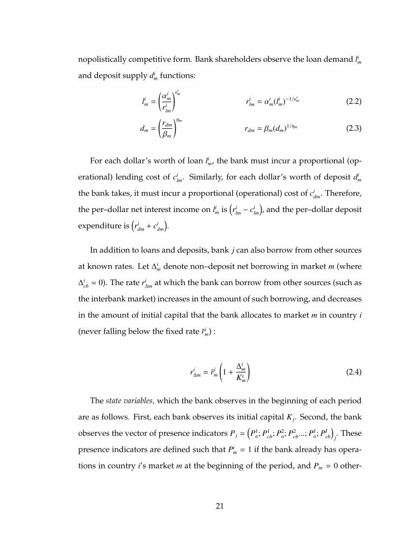
nopolistically competitive form. Bank shareholders observe the loan demand lim

and deposit supply dim functions:

lim =

(αi

m

rilm

)εim

rilm = αi

m(lim)−1/εi

m (2.2)

dm =

(rdm

βm

)ηm

rdm = βm(dm)1/ηm (2.3)

For each dollar’s worth of loan lim, the bank must incur a proportional (op-

erational) lending cost of cilm. Similarly, for each dollar’s worth of deposit di

m

the bank takes, it must incur a proportional (operational) cost of cidm. Therefore,

the per–dollar net interest income on lim is

(ri

lm − cilm

), and the per–dollar deposit

expenditure is(ri

dm + cidm

).

In addition to loans and deposits, bank j can also borrow from other sources

at known rates. Let ∆im denote non–deposit net borrowing in market m (where

∆icb = 0). The rate ri

∆m at which the bank can borrow from other sources (such as

the interbank market) increases in the amount of such borrowing, and decreases

in the amount of initial capital that the bank allocates to market m in country i

(never falling below the fixed rate rim) :

ri∆m = ri

m

(1 +

∆im

Kim

)(2.4)

The state variables, which the bank observes in the beginning of each period

are as follows. First, each bank observes its initial capital K j. Second, the bank

observes the vector of presence indicators P j =(P1

a; P1cb; P2

a; P2cb...; PI

a; PIcb

)j. These

presence indicators are defined such that Pim = 1 if the bank already has opera-

tions in country i’s market m at the beginning of the period, and Pm = 0 other-

21

wise 3. In addition to size and presence, the bank also brings its existing scope

of operations into the current period, which results from its optimal actions in

the preceding periods. This scope measures the extent to which the bank is able

to trade return for risk, and is captured by the lagged Sharpe ratio S j. Since

loan and deposit return indices are random and correlated across markets, this

scope measure S j captures the extent to which the bank can benefit from any

new entry/exit and investment choice.

The state variables(P j; S j

)depend on bank j’s previous entry/exit and quan-

tity choices. Since it is assumed that profits are re–distributed to shareholders

at the end of each period t, total asset size K j is taken to be exogenous from the

bank’s perspective. Further exogenous and known state variables of the model

are: the vectors of proportional lending and deposit taking costs; the vector of

taxes, capital and liquidity regulations (described below); the joint normal dis-

tribution of the return indices; the distribution of banks’ private shocks, and the

vectors of entry costs and scrap values, denoted by Γ and Ψ, respectively. Let Π

denote the set of all state variables.

Shareholders’ goal is to choose bank j’s portfolio so as to maximize mean–

variance utility over its end–period capital, denoted by K j. Let Kij denote the

end–period capital in country i. Due to the random shocks affecting the loan de-

mand and deposit supply functions, the country–specific Kij’s are also random

variables. In each country i, Kij is composed of the initial market capitalization

Kij, plus net loan interest income, minus deposit and non-deposit borrowing

expenditures, adjusted for the country–specific income tax ti.

Recall that cross-border loans come out of bank j’s domestic operations.

3Note that the subscript a refers to both affiliate loan and deposit markets

22

Fixed entry costs and scrap values appear in each affiliate’s end–period capi-

tal. These fixed costs are relevant only if bank j enters or exits market m in the

given period. Let eim j (Π) = 1 denote bank j’s decision to enter market m this pe-

riod, and em j (Π) = −1 is the decision to exit, conditional on all the state variables.

Then the domestic end–period capital is

Kusj = Kus

j + (1 − tus) · (rla − cla)usj · (l

usa j) − (rd + cd) · dus

j −

(r∆a · ∆a)usj +

∑i

(1 − ti

)· (rlcb − clcb)i

j ·(licb j

)−

∑i

Γicb

(1 : ei

cb j = 1)

+∑

i

Υicb

(1 : ei

cb j = −1)

(2.5)

Foreign affiliate income is repatriated to the bank’s domestic headquarters at

the repatriation tax rate of ωi. Then the country i foreign affiliate’s end–period

capital is4

Kij = Ki

j +(1 − ti

)·(1 − ωi

) (rla − cla)i

j · lia

− (rd + cd)ij · d

ij − (r∆a · ∆a)i

j

−Γi

a

(1 : ei

a j = 1)

+ Υia

(1 : ei

a j = −1)

(2.6)

After all foreign income is repatriated, bank j’s end–period aggregate capital is

K j =∑

i Kij.

Bank j’s activities are subject to minimum reserve and risk–weighted capital

requirements. Domestic and cross–border lending come out of the domestic

budget, and are therefore bound by domestic (U.S.) regulations. Foreign affiliate

operations are financed out of the budget of each foreign affiliate separately.

Therefore, foreign affiliate operations are bound by each foreign country i’s laws

4The loan revenue and deposit expenditure functions take the forms rilm · l

im =

(αi

m

)·(lim

) ε im−1ε i

m

and ridm · d

im =

(βi

m

)·(di

m

) ηim+1ηi

m respectively.

23

and regulations. Bank j can only operate (make loans and take deposits) in

market i if it starts with positive initial capitalization Kij > 0. Let δi denotes the

required reserve ratio, and ki denote the fixed minimum capital ratio in market

i. The budget constraints on bank j’s domestic and foreign affiliate operations

are

lusa j +

∑i

licb j ≤ Kus

j + ∆usa j + (1 − δus) · dus

j (2.7)

lia j ≤ Ki

j +(1 − δi

)· di

j + ∆ia j (2.8)

The bank regulator in country i considers banks’ risk–weighted capitalization in

its capital requirement. Let θi denote country i’s bank regulator’s risk aversion

parameter5, and V i is the variance–covariance matrix of the return indices in

country i alone.6 The risk–weighted capital requirements in the U.S. and coun-

try i are then

E[Kus

j

]−θus

2·(Kus′

j VusKusj

)≥ kus ·

lusa j +

∑i

licb j

(2.9)

E[Ki

j

]−θi

2·(Kus′

j VusKusj

)≥ ki ·

(lia j

)(2.10)

The budget and regulatory constraints must hold in each period and each

country. At this point it is useful to introduce time notation t.

Given the state Πt ∈ Π, banks choose actions simultaneously. The two types

of actions are the static loan/deposit quantity choices, and the dynamic foreign

market entry/exit choices. Recall that E j =(e j1...e jT

)denotes bank j’s actions,

and let Et = (e1t...eJt) denote the vector of time t actions. Then E = (E1...EJ).5This risk aversion parameter denotes the weight that the regulator puts on the market risk

on bank j’s portfolio6Note that the country–specific variance–covariance matrix of return indices V i is not the

same as the overall variance–covariance matrix on the bank’s portfolio, denoted by V in Equa-tion (2.15).

24

Before choosing its actions, each bank j receives a private shock ν jt, drawn inde-

pendently across banks and over time from a distribution G j (· | Πt) with support

ν j. The private shock might derive from variability in managerial drive for inter-

national portfolio diversification. Let the vector νt = (ν1t, ..., νJt) denote private

shocks of all banks.

Given its private shock, the entry/exit decision vector e j and the set of state

variables Πt, bank j’s utility takes the mean–variance form in each period t:

u(e j,Π, ν j

)t= E

(K j

)t−λ

2·(K′jVK j

)t

(2.11)

λ is the bank’s constant risk aversion, common across all banks. Letting γ < 1

denote the constant discount factor, we can write bank j’s discounted sum of

utilities over time as:

E

T∑t=0

γtu j

(e j,Π, ν j

)t| Πt

(2.12)

The expectation is over bank j’s private shock in the current period, as well as

future values of the state variables, actions, and private shocks. The final aspect

of the model is the transition between states. The state vector at date t + 1 is

denoted by Πt+1, and is drawn from a probability distribution Λ (Πt+1 | et,Πt).

The dependence of this function on et means that time t entry/exit decisions

affect the future strategic environment. However, not all states are influenced

by past actions.

The analysis of equilibrium behavior focuses on pure strategy Markov perfect

equilibria (MPE). In a MPE, each bank’s behavior depends only on the current

state. Formally, a Markov strategy for bank j is a functionω j: Π×ν j 7→ E j. A pro-

file of Markov strategies is a vector ω = (ω1, . . . , ωJ) where ω : (Π, ν1, . . . , νJ) 7→ E.

If behavior is given by a Markov strategy profileω, bank j’s expected utility over

25

time, given a state Π can be written recursively:

V j (Π, ω) = Eν

[u j

(ω (Π, ν) ,Πt, ν jt

)+ γ

∫V j

(Π′;ω

)dΛ

(Π′ | ω (Π, ν) ,Π

)| Π

](2.13)

In (2.13), V j is bank j’s ex ante value function in that it reflects expected prof-

its at the beginning of a period before private shocks are realized. The profile

ω is a Markov perfect equilibrium if, given the opponent profile ω− j, each bank

j prefers its strategy ω j to all alternative Markov strategies ω′j.That is, ω is a

Markov perfect equilibrium if for all banks j, states Π, and Markov strategies ω′j,

V j (Π, ω) ≥ V j

(Π;ω′j;ω− j

)(2.14)

It is assumed that all the conditions for the existence of such a MPE are satisfied.

2.3.2 Optimal Choices

Income from lending activities is redistributed to shareholders at the end of each

period. Therefore, bank j’s loan and deposit quantity choices can be analyzed in

a static, period by period setting. Accordingly, in each period t bank j chooses

its loan and deposit quantities to solve

maxlia j;l

icb j;d

ij∆

ij;K

ij

u(e j,Π, ν j

)t= E

(K j

)t−λ

2·(K′jVK j

)t

(2.15)

subject to the budget and regulatory constraints described in Equations (2.7)

through (2.10). Banks make optimal foreign market entry and exit decisions

that solve

maxe1 j,...,eM j

E

T∑t=0

γtu j

(e j,Π, ν j

)t| Πt

(2.16)

26

Given the vector of fixed entry costs Γ and scrap values Υ, the optimal mar-

ket entry and exit choices for a bank not in market i are as follows:Enter if V j

(ai

m j = 1; ai−m j,Π, ω

)− Γi

m ≥ V j

(ai

m j = 0; ai−m j,Π, ω

);

Stay out if otherwise.(2.17)

For a bank present in market i, the optimal decision rule is:Exit if V j

(ai

m j = −1; ai−m j,Π, ω

)+ Υi

m ≥ V j

(ai

m j = 0; ai−m j,Π, ω

);

Stay otherwise.(2.18)

This concludes the characterization of bank j’s optimal behavior. The next

section describes how to use the structure presented above to estimate the de-

terminants of banks’ optimal decisions.

2.4 Estimation

The purpose of this section is to use the model described above to estimate how

banks’ choices of foreign loans, as well as their market entry/exit decisions de-

pend on bank and market–specific characteristics. The goal is to recover the

model’s structural parameters. These parameters are: the utility function u (·),

the discount factor γ, the transition probabilities Λ (·), the regulatory and bank

risk aversion parameters (λ, θ), the tax rates and return indices (t,R), and the

proportional and fixed costs/scrap values (c,Γ,Υ).

In what follows, it is assumed that the unknown structural parameters are

the risk aversion parameters (λ, θ) and the fixed entry costs/scrap values (Γ,Υ).

Let Θ denote the set of unknown structural parameters such that Θ = (Γ,Υ, λ, θ).

27

The goal of the following estimation is to recover these structural parameters

from the model. The estimation strategy follows the Bajari, Benkard, and Levin

(2007) (BBL) method of estimating dynamic games of imperfect competition.

This method can estimate banks’ dynamic strategic choices in this model with-

out having to solve the dynamic optimization problem. The BBL method is

based on two underlying assumptions. First is the assumption that the model

described above represents banks’ true behavior. Second, it is conjectured that

the loan quantity and entry choices observed in the data result from banks’

utility–maximizing actions, given the bank and country–specific characteristics

(the state variables).

The estimation method consists of two parts. The first stage estimates bank

j’s optimal loan, deposit and entry/exit choices (the policy functions) as func-

tions of the set of time t state variables. That is, the first stage estimates:

(l∗; d∗; e∗) jt = f (Πt) (2.19)

where the ∗ superscript denotes observed optimal choices, and Πt is the set

of state variables as of time t. The regression in Equation (2.19) yields policy

function estimates(l; d; e

)for any state variable Πt. Plugging these estimates

into ut (·) produces the period by period value function. Transition probabilities

for the state variables are also needed. The entry/exit estimate e is in fact the

transition probability for bank j’s presence vector P. Transition probabilities of

the exogenous state variables can be estimated using observed data. As a result,

state transition probability function estimates Λ (Πt+1 | Πt) are obtained.

The second step uses the policy function estimates(l; d; e

)together with the

transition probability estimates Λ (Πt+1 | Πt) to forward-simulate values for the

discounted sum of utilities in (2.12). Recall that these estimates correspond to

28

banks’ optimal choices. Therefore, the resulting simulated value function cor-

responds to the value of banks’ optimal behavior. Importantly, the resulting

simulated values are still functions of the model’s unknown structural parame-

ters, such that V j (Π;ω;Θ).

Given(l; d; e

)together with Λ (Πt+1 | Πt), forward simulation can also be used

to evaluate any other (alternate) bank strategy ω′j, with corresponding simulated

values V j (Π;ω′;Θ). Based on the assertion that strategy ω j is bank j’s optimal

behavior (described in Equation (2.14) above), the following inequality must

hold at the true values of the structural parameters.

V j (Π;ω;Θ0) ≥ V j(Π;ω′;Θ0

)(2.20)

The second stage of the estimation then aims to find structural parameter

estimates Θ that minimize deviations from Equation (2.20). The detailed pro-

cess of getting the policy function estimates(l; d; e

)and the structural parameter

estimates Θ is described in the following subsections.

2.4.1 First Step: Policy Functions and Transition Probabilities

As described above, the first step consists of estimating banks’ policy functions

as functions of the period–specific state variables. The policy functions of in-

terest are the discrete entry/exit choices, and the continuous loan and deposit

quantity choices. Substituting estimates of these policy functions into the utility

function reflects on how the value of bank operations depend on state variables.

Estimation of the loan/deposit quantity choices and the foreign market en-

try/exit decisions can be achieved in one step, via the Heckman selection-bias-cor-

29

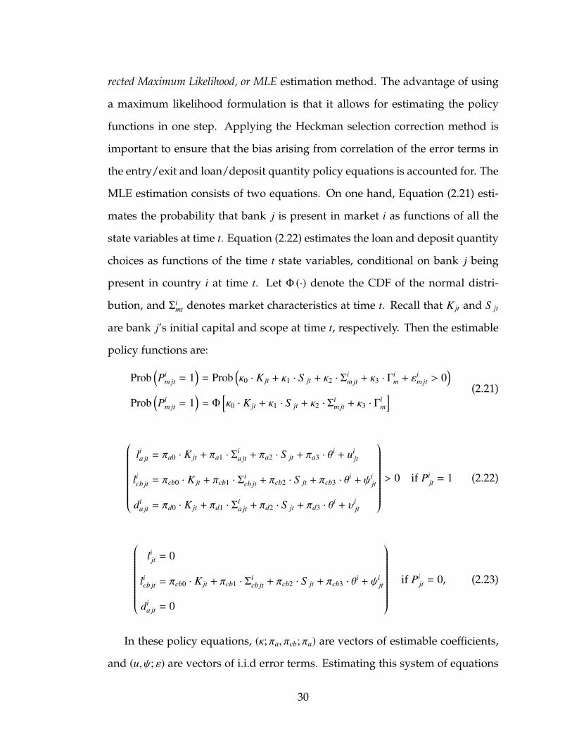
rected Maximum Likelihood, or MLE estimation method. The advantage of using

a maximum likelihood formulation is that it allows for estimating the policy

functions in one step. Applying the Heckman selection correction method is

important to ensure that the bias arising from correlation of the error terms in

the entry/exit and loan/deposit quantity policy equations is accounted for. The

MLE estimation consists of two equations. On one hand, Equation (2.21) esti-

mates the probability that bank j is present in market i as functions of all the

state variables at time t. Equation (2.22) estimates the loan and deposit quantity

choices as functions of the time t state variables, conditional on bank j being

present in country i at time t. Let Φ (·) denote the CDF of the normal distri-

bution, and Σimt denotes market characteristics at time t. Recall that K jt and S jt

are bank j’s initial capital and scope at time t, respectively. Then the estimable

policy functions are:

Prob(Pi

m jt = 1)

= Prob(κ0 · K jt + κ1 · S jt + κ2 · Σ

im jt + κ3 · Γ

im + εi

m jt > 0)

Prob(Pi

m jt = 1)

= Φ[κ0 · K jt + κ1 · S jt + κ2 · Σ

im jt + κ3 · Γ

im

] (2.21)

lia jt = πa0 · K jt + πa1 · Σ

ia jt + πa2 · S jt + πa3 · θ

i + uijt

licb jt = πcb0 · K jt + πcb1 · Σ

icb jt + πcb2 · S jt + πcb3 · θ

i + ψijt

dia jt = πd0 · K jt + πd1 · Σ

ia jt + πd2 · S jt + πd3 · θ

i + υijt

> 0 if Pi

jt = 1 (2.22)

li

jt = 0

licb jt = πcb0 · K jt + πcb1 · Σ

icb jt + πcb2 · S jt + πcb3 · θ

i + ψijt

dia jt = 0

if Pi

jt = 0, (2.23)

In these policy equations, (κ; πa, πcb; πa) are vectors of estimable coefficients,

and (u, ψ; ε) are vectors of i.i.d error terms. Estimating this system of equations

30

yields coefficient estimates φ = (κ; πa, πcb; πd). These estimates can be used to

derive predicted optimal entry/exit, loan and deposit quantity choices for any

combination of state variables Π. This is equivalent to obtaining estimates of the

optimal strategies ω (Πt; νt).

Estimation of the transition probabilities of the state variables in Π still re-

mains. Recall from above the eijt = 1 and ei

jt = −1 denote bank j’s decision to

enter and exit market i at time t, respectively. From Equation (2.21), it is straight-

forward to get transition probability estimates such that

Prob(ei

m jt = 1)

= Prob(Pi

m jt = 1 | Pim jt−1 = 0

)= Φ

(· | Pi

m jt−1 = 0)

Prob(ei

m jt = −1)

= Prob(Pi

m jt = 0 | Pim jt−1 = 1

)= 1 − Φ

(· | Pi

m jt−1 = 1) (2.24)

Estimates for the exogenous transition probabilities of bank capital K j can also

be obtained from the empirical distribution. The distribution of K j is normal.

Therefore, Monte Carlo simulation with a normal target distribution can simu-

late values for initial capital K.

The next section describes how to get estimates of the unknown structural

parameters Θ using the second step.

2.4.2 Second Step: Structural Parameter Estimates

Recall from above that the unknown structural parameters of interest are Θ =

(Γ,Υ, λ, θ). Estimates Θ are obtained from the second step of the estimation

method. The process of recovering these structural parameters goes as follows.

Using the estimated optimal strategies ω (Πt; νt) from the first step:

V j (Π;ω;Θ) = E

T∑t=0

γtu j

(ω (Πt; νt) ,Πt, ν jt; Θ

)| Π0 = Π; Θ

. (2.25)

31

Estimate V j (Π;ω;Θ) of the optimal value function can be obtained by forward–

simulation using the estimated transition probabilities Λ (·) as follows. Let N

denote the total number of simulations. Based on the first–stage policy function

estimates, bank j’s corresponding estimated optimal entry/exit decisions and

loan and deposit quantity choices — denoted by(l; d; e

)— are calculated and

plugged into u jt (·). These steps are repeated for each of T periods, using the es-

timated transition probabilities to govern state transitions. Bank j’s discounted

sum of utilities is then averaged over the many simulated paths (n = 1...N) to

yield the optimal value estimate V j (Π;ω;Θ).

The same process can simulate values for a number of sub–optimal strategy

paths ω′. Let V j (Π;ω′;Θ) denote the value estimates corresponding to these al-

ternate strategies. The final step is to use the value estimates V j (Π;ω;Θ) and

V j (Π;ω′;Θ) to set up inequalities which ensure that the observed bank actions

have the highest value. From Equation (2.20), it follows that

V j

(Π;ω j;ω− j;Θ0

)≥ V j

(Π;ω′;ω− j;Θ0

)(2.26)

The goal is to obtain estimates Θ to minimize violations of this set of inequalities.

It is assumed that all conditions ensuring point identification are satisfied. If the

set of inequalities characterizing the optimal choices is large enough and letting

x denote the equilibrium conditions, the following function captures deviations

from the set of inequalities in Equation (2.26):

g(x; Θ; φ

)= V j

(Π;ω j;ω− j;Θ; φ

)− V j

(Π;ω′;ω− j;Θ; φ

)(2.27)

Let gn

(x; Θ; φ

)be the value of this difference for the n’th simulation, when the

first–stage policy function parameter estimates are φ. Let nI denote the number

of sub–optimal policy paths examined (i.e. the number of inequalities) for each

32

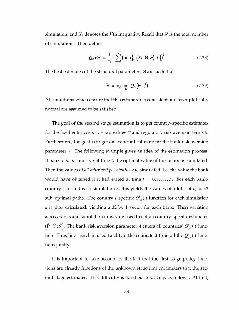
simulation, and Xk denotes the k’th inequality. Recall that N is the total number

of simulations. Then define

Qn (Θ) =1nI·

nI∑k=1

(min

g(Xk; Θ; φ

), 0

)2(2.28)

The best estimates of the structural parameters Θ are such that

Θ := arg minΘ

Qn

(Θ; φ

)(2.29)

All conditions which ensure that this estimator is consistent and asymptotically

normal are assumed to be satisfied.

The goal of the second stage estimation is to get country–specific estimates

for the fixed entry costs Γ, scrap values Υ and regulatory risk aversion terms θ.

Furthermore, the goal is to get one constant estimate for the bank risk aversion

parameter λ. The following example gives an idea of the estimation process.

If bank j exits country i at time t, the optimal value of this action is simulated.

Then the values of all other exit possibilities are simulated, i.e. the value the bank

would have obtained if it had exited at time t = 0, 1, . . . ,T . For each bank-

country pair and each simulation n, this yields the values of a total of nI = 32

sub–optimal paths. The country i–specific Qijn (·) function for each simulation

n is then calculated, yielding a 32 by 1 vector for each bank. Then variation

across banks and simulation draws are used to obtain country-specific estimates(Γi; Υi; θi

). The bank risk aversion parameter λ enters all countries’ Qi

jn (·) func-

tion. Thus line search is used to obtain the estimate λ from all the Qijn (·) func-

tions jointly.

It is important to take account of the fact that the first–stage policy func-

tions are already functions of the unknown structural parameters that the sec-

ond stage estimates. This difficulty is handled iteratively, as follows. At first,

33

the second–stage set of inequalities are solved using the observed loan and de-

posit quantities and entry/exit decisions as inputs (as opposed to first–stage

estimates). The resulting preliminary estimates of the structural parameters are

then used as explanatory variables in the first–stage policy function regressions.

The resulting policy function estimates are then used in the second stage to re–

estimate the structural parameters. The process is repeated until the parameter

estimates converge.

2.4.3 Data

The model’s equations are estimated on a panel data set constructed from quar-

terly data on activities of U.S. banks in 46 foreign markets. The data cover

the period between 1997 Q4 to 2005 Q4, a total of 33 quarters. Data on U.S.

Banks’ foreign claims and liabilities are from the Federal Financial Institutions

Examination Council (FFIEC) Country Exposure Surveys. This quarterly sur-

vey reports on the foreign activities of U.S. banks with foreign exposure over

30 million USD broken down by host country. Data are reported separately

for three bank size groups: Money Center Banks (large); Other Large Banks

(medium) and All Other Banks (small). Data were collected from these surveys

on U.S. banks’ (1) domestic (U.S.) claims; and for each host country separately:

(2) cross–border claims; (3) foreign affiliate claims, and (4) foreign affiliate lia-

bilities.7 The data are reported on an immediate counter–party basis, i.e. they

do not take account of cross–country risk transfers. For each bank size category,

the reported total claims and liabilities were divided by the number of banks to

obtain the averageloan and deposit quantities. This is necessary since the num-7The reported survey data were converted into millions of USD, using 2005 Q4 as the base

for inflation adjustment.

34

ber and total asset size of reporting banks change significantly over time within

the panel.

With respect to the model parameters, data were collected on bank size (total

assets) from the FFIEC Surveys described above. Data on the market–specific

model parameters for the 46 host markets were gathered from various sources,

including the International Monetary Fund (1997-2005)’s International Finan-

cial Statistics, Organisation for Economic Co-operation and Development (1997-

2005)’s Statistics, the Economist Intelligence Unit (1997-2005)’s Country Data

and the World Bank (1997-2005)’s Bank Regulation and Supervision database.

Initial values of the second stage estimation described in the earlier sections

use bank and regulatory risk aversion parameter value estimates from the re-

lated literature. Previous papers have reported banks’ risk aversion parameter

(captured by λ) to be in the 0.20 (Nishiyama, 2007) to 0.29 (Kuhn, 2006) range.

For the entry costs, starting values come from regressing total costs on the total

volume of activities for each country. The constant term from this regression

provides a good initial value of the entry cost.

2.5 Estimation Results

2.5.1 Market Entry/Exit Choices and Loan/Deposit Quantities

This section describes the results of the static policy function estimations, which

correspond to the first stage described above. The policy choices of interest are

the affiliate loans, cross–border loans and deposits, as well as the entry and exit

35

decisions in each country. The results of the Maximum Likelihood policy func-

tion estimation with the Heckman selection correction are presented in Tables

2.1 and 2.2.

The foreign market entry and exit results in Table 2.1. show that higher ex-

pected returns encourage entry and discourage exit. Furthermore, higher taxes,

costs and stricter foreign market regulations discourage entry and increase the

probability that banks leave the market. Both bank size and bank scope have

strong positive impacts on the probability of entry, and significantly discourage

exit. However, it is interesting to note that the scope effect is more than twice as

large as the size effect. Regulatory risk aversions only have small and insignifi-

cant impacts on the entry/exit choices of banks. Higher entry costs significantly

discourage entry, and greater scrap values increase the probability that banks

exit the market.

The policy function estimates corresponding to the first stage of the estima-

tion give strong confirmation of the importance of the selection bias in banks

foreign activities. The correlation of the error terms of the selection and volume

(quantity) equations is significant and positive with ρ = 0.31∗∗∗(.02). This result

implies that on average, banks lend 32.98 percent more in selected markets, compared

to a random sample of countries. This significant and positive correlation, together

with the fact that most explanatory variables impact both the entry/exit, as well

as the volume choices, implies that the coefficient estimates suffer from serious

upward bias. Specifically, running ordinary least squares regressions on the

loan and deposit volumes (ignoring the selection bias) would lead us to over-

state the impact of model variables. For instance, greater bank size makes banks

more likely to enter a new market, and also increases the loan and deposit vol-

36

umes, once there. OLS regression would therefore assign bank size a large coef-

ficient, combining the impacts of size on entry and volume, conditional on entry.

For comparison, the OLS coefficient estimate for the impact of bank size on affil-

iate loan volumes is 1.42, which is 12.7 percent higher than the true coefficient of

1.26 shown in Table 2.1. On average, affiliate loan volume coefficient estimates

suffer from an upward selection bias of 12.72 percent, while the average bias in

deposit coefficients is 12.47 percent.

Table 2.2 shows the bias-corrected coefficient estimates for banks’ choices of

cross–border loan, foreign affiliate loan and deposit volumes. Higher expected

returns encourage banks to increase their loan volumes. Higher deposit financ-

ing costs have strong negative effects on deposit and affiliate loan volumes.

This latter result confirms the importance of deposit–financing for affiliate loans.

Stricter capital regulations have significant negative impacts on all foreign ac-

tivities, with the strongest discouraging effect on affiliate loans. As expected,

more competitive loan markets tend to increase loan volumes. It is surprising

that deposit volume decreases as banks face more elastic deposit supply curves.

Both bank size and bank scope have strong positive impacts on loan and deposit

volumes. It is interesting that bank scope has over three times as large an impact

as bank size. This difference is most expressed for cross–border loan volumes,

where the scope effect is over eight times the size of the bank size effect.

In what follows, the transition probabilities for the presence vector P are

constructed using coefficient estimates from Table 2.1. The paths for bank asset

size K j are constructed using Monte Carlo draws from the empirical normal

distribution with the following bank size–specific moments. For small banks,

the empirical distribution is characterized by N (10, 0.07). For the medium-size

37

Table 2.1: Foreign Market Entry & Exit Probabilities: Elasticities.

Explanatory Variables Entry Probability Exit Probability

Exp Affil Loan Rate 0.86∗(.49) −0.03∗(.02)

Exp Deposit Rate −0.32 (1.01) 0.01 (.04)

Income Tax Rate −2.57∗∗∗(.49) 0.10∗∗∗(.02)

Lending Cost −0.08∗∗(0.04) 0.01∗∗(.00)

Minimum Capital Ratio −1.44∗∗∗(.31) 0.05∗∗∗(.01)

Required Reserve Ratio −0.01 (.04) 0.01 (.00)

Lagged Bank Size 0.73∗∗∗(.04) −0.03∗∗∗(.00)

Affil Loan Demand Elast 0.28∗∗∗(.05) −0.01∗(.00)

Deposit Supply Elast −0.08∗∗(.04) 0.01∗∗(.00)

Lagged Sharpe Ratio 1.70∗∗(.78) −0.06∗∗(.03)

Regulatory Risk Aversion −0.01 (.05) 0.01 (.00)

Fixed Entry Cost −0.20∗∗(.09) 0.01∗∗(.00)

Fixed Scrap Value 0.06∗(.04) 0.01∗∗∗(.00)

38

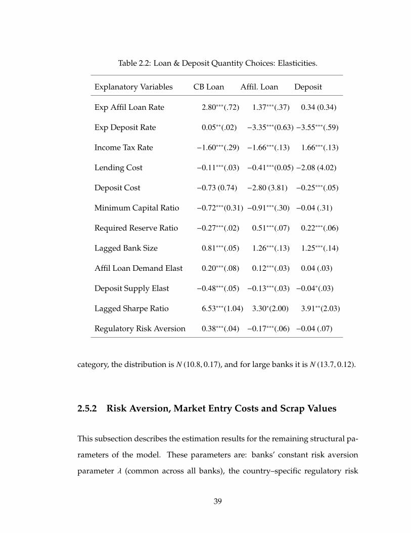
Table 2.2: Loan & Deposit Quantity Choices: Elasticities.

Explanatory Variables CB Loan Affil. Loan Deposit

Exp Affil Loan Rate 2.80∗∗∗(.72) 1.37∗∗∗(.37) 0.34 (0.34)

Exp Deposit Rate 0.05∗∗(.02) −3.35∗∗∗(0.63) −3.55∗∗∗(.59)

Income Tax Rate −1.60∗∗∗(.29) −1.66∗∗∗(.13) 1.66∗∗∗(.13)

Lending Cost −0.11∗∗∗(.03) −0.41∗∗∗(0.05) −2.08 (4.02)

Deposit Cost −0.73 (0.74) −2.80 (3.81) −0.25∗∗∗(.05)

Minimum Capital Ratio −0.72∗∗∗(0.31) −0.91∗∗∗(.30) −0.04 (.31)

Required Reserve Ratio −0.27∗∗∗(.02) 0.51∗∗∗(.07) 0.22∗∗∗(.06)

Lagged Bank Size 0.81∗∗∗(.05) 1.26∗∗∗(.13) 1.25∗∗∗(.14)

Affil Loan Demand Elast 0.20∗∗∗(.08) 0.12∗∗∗(.03) 0.04 (.03)

Deposit Supply Elast −0.48∗∗∗(.05) −0.13∗∗∗(.03) −0.04∗(.03)

Lagged Sharpe Ratio 6.53∗∗∗(1.04) 3.30∗(2.00) 3.91∗∗(2.03)

Regulatory Risk Aversion 0.38∗∗∗(.04) −0.17∗∗∗(.06) −0.04 (.07)

category, the distribution is N (10.8, 0.17), and for large banks it is N (13.7, 0.12).

2.5.2 Risk Aversion, Market Entry Costs and Scrap Values

This subsection describes the estimation results for the remaining structural pa-

rameters of the model. These parameters are: banks’ constant risk aversion

parameter λ (common across all banks), the country–specific regulatory risk

39

aversion parameters θi, and the country–specific entry costs Γi and scrap val-

ues Υi (which are common across banks and constant over time). The estimates

presented in the following tables result from the second stage of the estimation.

It is important to emphasize that the estimation aims to capture entry costs

and scrap values that are fixed — i.e. fundamentally independent of the scope

and scale of banks’ activities in each market. However, costs associated with

branch network building are inherently proportional to the scale of banks’ ac-

tivities. Therefore, proportional total operating costs (including branch network costs)

are subtracted from interest revenue, in order to make the fixed cost estimates

scale–independent. The estimate for the bank risk aversion parameter is λ =

0.34∗∗∗(.00). Table 2.3 presents the fixed entry cost, scrap value and regulatory

risk aversion parameter estimates for each country in the sample, and Table 2.4

examines how estimates correlate with economic and regulatory measures.

As shown in Table 2.5, scale–independent entry costs and scrap values are

moderate with averages of 1.12 and 0.56 million USD, respectively. Entry costs

and scrap values show clear regional patterns. Table 2.3 shows that entry costs

appear to be the highest in the Eastern European countries — notably in Hun-

gary, the Czech Republic and Russia. These costs are also above average in the

South–East Asian economies, and appear low in most European countries and

the rest of the developed world. The scrap values are consistently lower than

the entry cost estimates, as expected. Scrap values are positively correlated with

entry costs in the OECD states. In developing countries, however, higher en-

try costs are accompanied by average scrap values. Scrap values are generally

higher in markets where market exit was observed, highlighting the positive re-

lationship between scrap values and market exit (also documented in Table 2.1).

40

Table 2.3 also presents the estimated regulatory risk aversion parameters. Table

2.5 shows that with a mean risk aversion parameter estimate of 0.52, regulators

are generally more risk averse than banks. Regulatory risk aversion estimates

are the highest in the South American states, while European and North Amer-

ican regulators appear to have risk aversions below average.

Table 2.3 shows that for the South American countries in the sample, vari-

ation in the simulated data was not sufficient to provide entry cost estimates.

The forward simulation was successful in getting estimates for most countries’

regulatory risk aversion and scrap values.

Table 2.3: Estimates of Entry Costs, Scrap Values (Millions of 2004 Q4USD) and Risk Aversions.

Country Entry Cost Scrap Value Reg. Risk Aversion

Argentina − 0.94∗∗∗(.03) 1.19∗∗∗(0.29)

Australia 0.87∗∗∗(.03) 0.09∗∗∗(.01) 0.31∗∗∗(.11)

Austria 0.29∗∗∗(.01) − 0.35∗∗∗(.06)

Belgium 0.77∗∗∗(.10) 0.44∗(.23) 0.25∗∗(.14)

Brazil − 1.29∗∗∗(.42) 0.40(.43)

Bulgaria 0.70∗∗∗(.03) 0.60∗∗∗(.02) 0.78∗∗∗(.18)

Canada 0.85∗∗∗(.10) 0.31(.57) 0.24(.41)

Chile − 0.79(.74) 0.70∗∗∗(.22)

China 0.43∗∗∗(.03) 0.04(.03) 0.75(.56)

41

Table 2.3: (Continued)

Country Entry Cost Scrap Value Reg. Risk Aversion

Columbia − 0.41∗∗∗(.01) 0.79(.71)

Czech Rep. 4.23∗∗∗(.10) 0.64∗∗∗(.06) 0.01∗∗∗(.00)

Denmark 0.90∗∗∗(.03) − 0.51∗∗∗(.06)

Finland 0.93∗∗∗(.03) 0.12∗∗∗(.01) 0.50∗∗∗(.06)

France 0.85∗∗∗(.05) 0.77∗∗∗(.02) 0.70∗∗∗(.14)

Germany 1.12∗∗∗(.08) 0.11∗∗∗(.02) 0.43∗∗∗(.12)

Greece − 0.88∗∗∗(.14) 0.52∗(.30)

Hungary 2.05∗∗∗(.16) 0.65∗∗∗(.02) 0.03(.24)

Iceland − 1.60∗∗∗(.08) 0.59(.63)

India 1.59∗∗∗(.17) 1.20∗∗∗(.14) 0.20∗∗∗(.07)

Indonesia − 1.12∗∗∗(.24) 0.42∗(.28)

Ireland 0.93∗∗∗(.04) 0.26∗∗∗(.01) 0.45∗∗∗(.06)

Israel − 0.71∗∗∗(.04) 0.49(.58)

Italy 0.87∗∗∗(.03) 0.83∗∗∗(.03) 0.52∗∗∗(.06)

Japan 0.94∗∗∗(0.08) 0.13∗∗∗(.03) 0.40∗∗∗(.12)

Luxembourg 1.01∗∗∗(.09) 0.11∗∗∗(.02)) 0.33∗∗∗(.10)

Malaysia 0.30∗∗∗(.01) 0.02∗∗∗(.01) 0.90 (.60)

Mexico 0.85∗∗∗(.04) 0.12∗∗∗(.01) 0.68∗∗∗(.12)

Netherlands 0.30∗∗∗(.01) 0.03∗∗∗(.01) 0.63 (.68)

42

Table 2.3: (Continued)

Country Entry Cost Scrap Value Reg. Risk Aversion

New Zealand 0.98∗∗∗(.06) 0.11∗∗∗(.01) 0.42∗∗∗(.09)

Norway 0.89∗∗∗(.03) 0.13∗∗∗(.01) 0.49∗∗∗(.06)

Philippines − 1.19∗∗∗(.06) 0.64∗∗∗(.10)

Poland − 0.98∗∗∗(.05) 0.56∗∗∗(.13)

Portugal − 1.10∗∗∗(.30) 0.42 (.39)

Romania − 0.96∗∗∗(.09) 0.60∗∗∗(.19)

Russia 5.16∗∗∗(.39) 0.89∗∗(.29) 1.06 (1.21)

Slovakia − 0.97∗∗∗(.08) 0.64∗∗∗(.19)

South Africa − 0.88∗∗∗(.15) 0.57∗(.33)

South Korea 1.05∗∗∗(.08) 0.11∗∗∗(.02) 0.36∗∗∗(.10)

Spain 0.87∗∗∗(.03) 0.10 (.01) 0.46∗∗∗(.06)

Sweden 0.88∗∗∗(.04) 0.13∗∗∗(.00) 0.48∗∗∗(.06)

Switzerland 0.80∗∗∗(.02) 0.09∗∗∗(.00) 0.54 (.38)

Thailand 0.17∗∗∗(.01) 0.04∗∗∗(.01) 0.71 (1.14)

Turkey − 1.12∗∗∗(.22) 0.43 (.31)

United Kingdom 0.86∗∗∗(.07) 0.14∗∗∗(.03) 0.50∗∗∗(.14)

United States − − 3.91 (13.6)

Table 2.4 correlates the parameter estimates with numerous empirical indi-

cators of bank profitability, efficiency, economic openness and political and reg-

43

ulatory background. Estimated entry costs are significantly higher in markets

that are inefficient, profitable, risky, have a greater share of government own-

ership, and where the banking sector is less developed. Scrap values show the

same pattern. It is interesting that the gap between entry costs and scrap values

is greater in markets that are more profitable with less developed banking sec-

tors. The regulatory risk aversion estimates are significantly higher in markets

that are inefficient and less developed. Higher overhead costs in markets with

more risk averse regulators might be due to a greater burden of compliance.

Furthermore, regulatory risk aversion estimates are strongly positively corre-

lated with other measures of bank regulations, such as minimum capital ratios

and liquidity regulations. Regulators appear more risk averse in markets where

they have less corrective power with respect to existing regulations.

Table 2.4: Correlations with Economic and Regulatory Measures.

Measures Entry Cost Scrap Value Entry-Scrap Reg. Risk A.

Entry Cost 1.00

Scrap Value 0.55 1.00

Entry Minus Scrap 0.96∗∗∗ 0.29 1.00

Reg. Risk Aversion −0.07 0.06 −0.05 1.00

Cap-Acct Open-Index −0.22 −0.35∗∗ 0.01

Distance from U.S. −0.04 −0.06 −0.03 −0.02

44

Table 2.4: (Continued)

Measures Entry Cost Scrap Value Entry-Scrap Reg. Risk A.

Common Language −0.05 −0.07 −0.10 −0.22

Average Total Costs 0.40∗∗ 0.05 0.42∗∗ −0.28∗

Avg Overhead Costs 0.52∗∗∗ 0.47∗∗∗ 0.53∗∗∗ 0.43∗∗∗

Total Banking Cost −0.14 −0.13 −0.16 −0.13

ICRG Comp Risk −0.36∗∗ −0.60∗∗∗ −0.21 −0.28∗

ICRG Fin. Risk −0.12 −0.55∗∗∗ −0.07 −0.16

Govt ownship Share 0.49∗∗∗ 0.52∗∗∗ 0.37∗ 0.12

Bank Development −0.45∗∗∗ −0.62∗∗∗ −0.35∗ −0.07

Net Interest Margin 0.55∗∗∗ 0.61∗∗∗ 0.53∗∗∗ 0.14

Nonperf. Loan Share 0.43∗∗∗ 0.17 0.37 0.15

Socialist Legal Origin 0.70∗∗∗ 0.18 0.70∗∗∗ −0.02

OECD Member −0.16 −0.37∗∗ −0.11 −0.47∗∗∗

Corrective Power −0.11 0.26 −0.12 −0.52∗∗∗

Min. Capital Ratio 0.24 0.46∗∗ 0.17 0.28∗

Req. Reserve Ratio 0.07 0.19 −0.02 0.32∗∗

45

Table 2.5: Summary Statistics For Estimation Results.

Estimates Min 25p 50p 75p Max Mean Std Dev

Reg. Risk Aversion 0.01 0.42 0.50 0.64 1.19 0.52 0.23

Entry Cost 0.17 0.80 0.88 1.01 5.16 1.12 1.05

Scrap Value 0.02 0.11 0.44 0.94 1.91 0.56 0.49

2.6 Simulation Exercises

This section conducts four types of exercises. Subsection 2.6.1.examines the ef-

fect on banks’ optimal behavior of gradually increasing the bank risk aversion

parameter λ, while holding all countries’ regulatory risk aversion parameters

constant at their estimated values. Subsection 2.6.2 examines the effects of in-

creasing all foreign countries’ risk aversion parameters simultaneously, holding

the bank risk aversion λ and the U.S. regulatory risk aversion constant at their

estimated values. Subsection 2.6.3 analyzes the impact of gradual increases in

the U.S. regulator’s risk aversion parameter, while holding λ and all other mar-

kets’ regulatory risk aversion constant. Recall that bank risk aversion is the

weight banks put on the variance of their global portfolios. Furthermore, for-

eign regulatory risk aversion is the weight each country’s bank regulator puts

on the variance of banks’ country–specific portfolios. Finally, U.S. regulatory

risk aversion is the weight the U.S. bank regulator attaches to the variance of

U.S. banks’ domestic portfolios.

46

2.6.1 Increasing Bank Risk Aversion

Figures 2.1 through 2.4 show the effects of raising the bank risk aversion param-

eter λ from 0.001 to 4, holding all regulatory risk aversion parameters constant at

their estimated values. For each λ, the value of the banks’ problem is evaluated

0 1 2 3 44.2

4.3

4.4

4.5

4.6

4.7

4.8

4.9x 106

Bank Risk Aversion.

Val

ue o

f Glo

bal O

ps.

Avg. Value ofGlobal Ops.

Figure 2.1: Value of Banks’Global Portfolio as Function of Bank Risk Aver-sion.

at the corresponding fixed entry costs and scrap values.

Figure 2.1 shows that λ has a strong negative impact on the value of the

bank’s global operations. As λ increases from 0.001 to 4, the bank’s simulated

value falls 12 percent. Figure 2.2 depicts the effect of increases in λ at the aver-

age country level. Figure 2.2 shows that both the value of banks’ U.S. operations,

and the average value of foreign country–specific operations are negatively af-

fected. As λ increases from 0.001 to 4, the value of U.S. operations falls 5.1

percent, while the average value of foreign country operations falls 5 percent. It

47

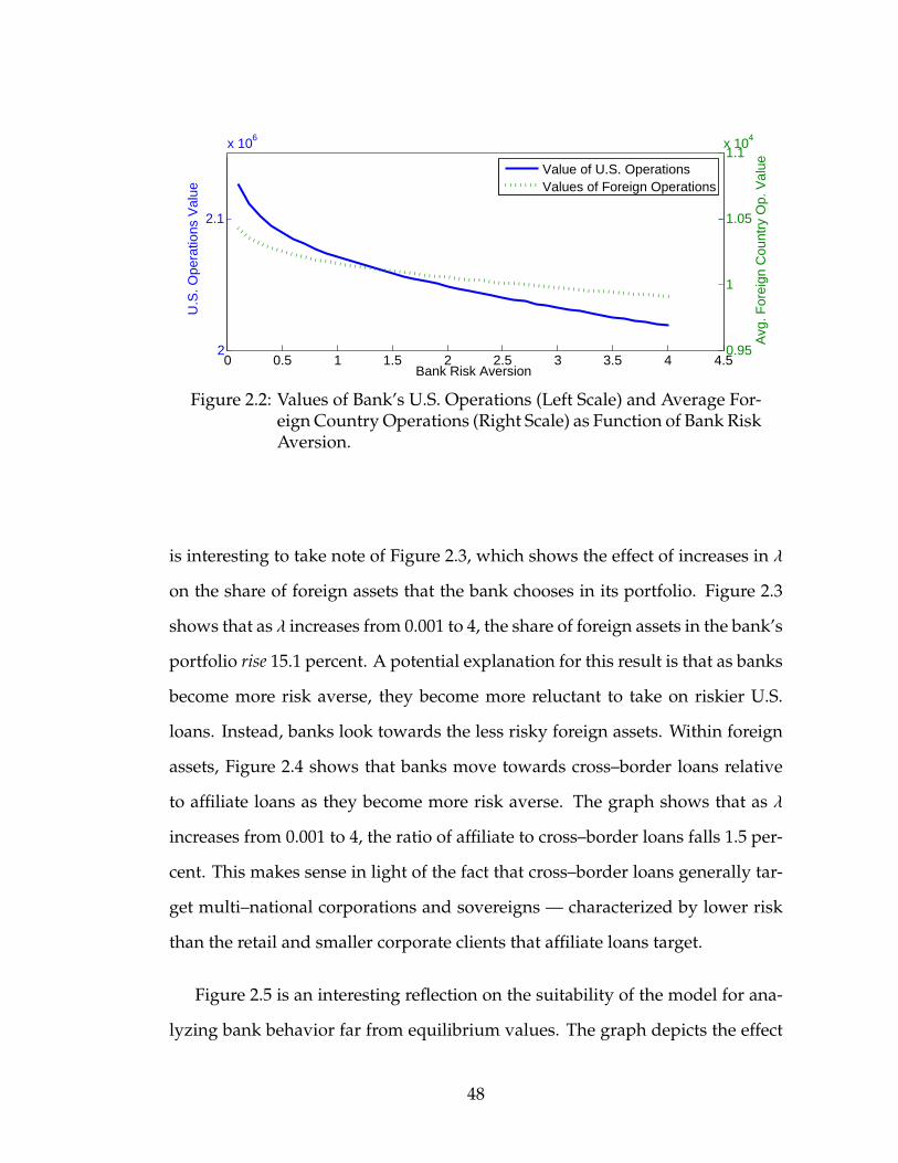
0 0.5 1 1.5 2 2.5 3 3.5 4 4.52

2.1

x 106

Bank Risk Aversion

U.S

. Ope

ratio

ns V

alue

0 0.5 1 1.5 2 2.5 3 3.5 4 4.50.95

1

1.05

1.1x 104

Avg

. For

eign

Cou

ntry

Op.

Val

ueValue of U.S. OperationsValues of Foreign Operations

Figure 2.2: Values of Bank’s U.S. Operations (Left Scale) and Average For-eign Country Operations (Right Scale) as Function of Bank RiskAversion.

is interesting to take note of Figure 2.3, which shows the effect of increases in λ

on the share of foreign assets that the bank chooses in its portfolio. Figure 2.3

shows that as λ increases from 0.001 to 4, the share of foreign assets in the bank’s

portfolio rise 15.1 percent. A potential explanation for this result is that as banks

become more risk averse, they become more reluctant to take on riskier U.S.

loans. Instead, banks look towards the less risky foreign assets. Within foreign

assets, Figure 2.4 shows that banks move towards cross–border loans relative

to affiliate loans as they become more risk averse. The graph shows that as λ

increases from 0.001 to 4, the ratio of affiliate to cross–border loans falls 1.5 per-

cent. This makes sense in light of the fact that cross–border loans generally tar-

get multi–national corporations and sovereigns — characterized by lower risk

than the retail and smaller corporate clients that affiliate loans target.

Figure 2.5 is an interesting reflection on the suitability of the model for ana-

lyzing bank behavior far from equilibrium values. The graph depicts the effect

48

0 1 2 3 40.125

0.13

0.135

0.14

0.145

0.15

Bank Risk Aversion

For

eign

Ass

ets

Sha

re

Avg. Share ofForeign Assets

Figure 2.3: Share of Foreign Assets in Bank’s Portfolio as Function of BankRisk Aversion.

of increases in λ on the estimated average fixed costs of entry and scrap values.

The graph shows that these estimated costs and scrap values remain constant

until λ reaches 2.4, and increase sharply thereafter. As λ increases from 2.4 to

4, average estimated fixed entry costs rise 23 percent, and scrap values increase

by 65 percent. In light of the fact that there is no reason to expect fixed costs

and scrap values to vary with λ, Figure 2.5 shows that the model behaves well

up to approximately eight times the equilibrium value of λ = 0.34. Beyond that,

however, the model produces unreliable results.

49

0 0.5 1 1.5 2 2.5 3 3.5 4 4.50.518

0.52

0.522

0.524

0.526

0.528

0.53

0.532

Bank Risk Aversion

Affi

liate

Loa

n to

CB

Loa

n R

atio

Aff Loan to CB LoanRatio − All Banks

Figure 2.4: Ratio of Affiliate Loans to Cross-border Loans in Bank’s Port-folio as Function of Bank Risk Aversion.

0 0.5 1 1.5 2 2.5 3 3.5 4 4.51

1.2

1.4

1.6

Bank Risk Aversion

Fix

ed E

ntry

Cos

t

0 0.5 1 1.5 2 2.5 3 3.5 4 4.50.4

0.6

0.8

1

Fix

ed S

crap

Val

ue

Avg. Scrap ValueAvg Entry Cost

Figure 2.5: Average Estimated Fixed Entry Costs and Scrap Values asFunction of Bank Risk Aversion.

50

2.6.2 Increasing Foreign Regulatory Risk Aversion

Regulatory and bank risk aversion work through different channels; bank risk

aversion through the objective function and regulatory risk aversion through a

constraint. This subsection explores the effects of varying all foreign markets’

regulatory risk aversions simultaneously, while keeping the bank risk aversion

and U.S. regulatory risk aversion parameters constant at their estimated values.

0 0.5 1 1.5 2 2.5 3 3.5 4 4.54.67

4.68

4.69

4.7

4.71

4.72

4.73

4.74x 106

Foreign Regulatory Risk Aversion

Val

ue o

f Glo

bal O

pera

tions

Avg. Value ofGlobal Operations

Figure 2.6: Value of Banks’ Global Portfolio as Function of Foreign Regu-latory Risk Aversion.

Figure 2.6 shows that as all foreign markets’ regulatory risk aversions in-

crease from 0.001 to 4, the value of global operations increases moderately by 1.3

percent. Figure 2.7 shows that a similar increase in foreign θ causes the value of

the bank’s U.S. operations to increase slightly by 1.9 percent, and the value of

the average foreign country operation to fall by 3.6 percent. Figure 2.8 depicts

51

the strong negative relationship between foreign θ and the share of foreign as-

sets in the bank’s portfolio. As foreign θ increases from 0.001 to 4, the share of

foreign assets falls by 21.4 percent. Therefore, stricter foreign bank regulations

cause U.S. banks to adopt a much more domestic focus.

0 0.5 1 1.5 2 2.5 3 3.5 4 4.52

2.05

2.1

2.15

2.2x 106

Foreign Regulatory Risk Aversion

U.S

. Ope

ratio

ns V

alue

0 0.5 1 1.5 2 2.5 3 3.5 4 4.51

1.02

1.04

1.06

1.08

1.1x 104

Ave

rage

For

eign

Cou

ntry

Op.

Val

ue

Value of U.S. OperationsAvg. Value of ForeignCountry Operations

Figure 2.7: Values of Banks’ U.S. Operations (Right Scale) and AverageForeign Country Operations (Right Scale).

Figure 2.9 depicts the effect of increases in foreign θ on the ratio of affiliate

loans to cross–border loans in the bank’s portfolio. As foreign θ rises up to

4, this ratio decreases significantly by 40.3 percent. Therefore, while stricter

foreign regulations lower foreign participation of U.S. banks altogether, foreign

affiliate assets take a much greater hit relative to cross–border loans. This result

is likely due to the fact that affiliate loans are generally under foreign regulators’

supervision, while the regulation of cross–border loans is often shared by the

U.S. and foreign regulators. Therefore, a stricter foreign regulatory framework

affects affiliate assets to a greater extent.

52

0 0.5 1 1.5 2 2.5 3 3.5 4 4.50.12

0.125

0.13

0.135

0.14

0.145

0.15

0.155

0.16

0.165

Foreign Regulatory Risk Aversion

For

eign

Ass

et S

hare

Avg Share of Foreign Assets

Figure 2.8: Share of Foreign Assets in Banks’ Portfolio as Function of For-eign Regulatory Risk Aversion.

0 0.5 1 1.5 2 2.5 3 3.5 4 4.50.35

0.4

0.45

0.5

0.55

0.6

0.65

0.7

Foreign Regulatory Risk Aversion

Affi

liate

Loa

n to

CB

Loa

n R

atio

Avg. Ratio of Affil toCB Loans

Figure 2.9: Ratio of Affiliate Loans to Cross-border Loans in Banks’ Port-folio as Function of Foreign Regulatory Risk Aversion.

53

2.6.3 Increasing U.S. Regulatory Risk Aversion

This chapter focuses on the behavior of U.S. banks exclusively. Therefore, it

is particularly interesting to analyze how banks’ optimal behavior changes, as

the U.S. regulators become more risk-averse. This subsection explores the ef-

fects of increasing the risk aversion of U.S. regulators on banks’ optimal behav-

ior. In this exercise, bank risk aversion and all other markets’s regulatory risk

0 0.5 1 1.5 2 2.5 3 3.5 4 4.54.05

4.1

4.15

4.2

4.25

4.3

4.35x 106

U.S. Regulatory Risk Aversion

Val

ue o

f Glo

bal

Ope

ratio

ns

Avg. Value ofGlobal Operations

Figure 2.10: Value of Banks’ Global Portfolio as Function of U.S. Regula-tory Risk Aversion.

aversions are held constant at their estimated values. Figure 2.10 shows the re-

lationship between the simulated value of the bank’s global operations as the

U.S. regulatory risk aversion θ increases from 0.001 to 4. This increase in U.S.

θ causes the value of the bank’s global operations to fall by 5.5 percent. Figure

2.11 focuses on the country–specific effects of the increase in U.S. θ, depicting

the results for the value of U.S. operations and the value of the average foreign

54

0 0.5 1 1.5 2 2.5 3 3.5 4 4.51.5

1.55

1.6

1.65x 106

U.S. Regulatory Risk Aversion

U.S

. Ope

ratio

ns V

alue

0 0.5 1 1.5 2 2.5 3 3.5 4 4.56500

7000

7500

8000

For

eign

Cou

ntry

Op.

Val

ue

Avg Value of ForeignCountry OperationsValue of U.S. Operations

Figure 2.11: Value of Banks’ U.S. Operations (Left Scale) and Average For-eign Country Operations (Right Scale).

country operations. The increase in U.S. θ from 0.001 to 4 causes the value of U.S.

operations to fall by 8.2 percent, and the value of the average foreign country

operation rises by 7.9 percent.

It is interesting to note Figure 2.12’s depiction of the strong positive relation-

ship between the share of foreign assets in the bank’s portfolio and U.S. θ. As

U.S. θ increases from 0.001 to 4, the share of foreign assets in the bank’s global

portfolio increases by 38 percent. Therefore, a stricter U.S. bank regulatory en-

vironment causes U.S. banks to take a more international focus. An increase in

U.S. θ from 0.001 to 4 does not have a notable impact on the ratio of affiliate

loans to cross–border loans in the bank’s global portfolio.

It is also insightful to compare and contrast how U.S. banks’ foreign focus re-

sponds to changes in U.S. versus foreign regulatory strictness. Based on the last

two simulation exercises, it appears that stricter U.S. regulations encourage U.S.

55

0 0.5 1 1.5 2 2.5 3 3.5 4 4.50.105

0.11

0.115

0.12

0.125

0.13

0.135

0.14

0.145

0.15

U.S. Regulatory Risk Aversion

For

eign

Ass

et S

hare

Share of Foreign Assetsin Portfolio

Figure 2.12: Share of Foreign Assets in Banks’ Portfolio as Function of U.S.Regulatory Risk Aversion.

banks’ foreign participation to a greater extent than stricter foreign regulations

discourage them. However, foreign regulations have a very strong impact on

the composition of U.S. banks’ foreign portfolio (greatly discouraging affiliate

lending), while U.S. regulations play only a very small role in these considera-

tions.

2.7 Summary

This chapter examines the determinants of U.S. banks’ international portfolio

choices, with the goal of recovering the underlying structural parameters that

shape these decisions. It presents a dynamic model of mean–variance utility

maximizing monopolistically competitive bank behavior. Banks make period–

by–period choices of optimal domestic, cross–border and foreign affiliate loan

and deposit quantities. In addition, banks make foreign market entry/exit deci-

56

sions considering their lifetime utility. All these decisions are bound by budget

and regulatory constraints, and depend on period–specific state variables such

as bank characteristics (initial size and scope) and market traits (return indices,

correlations, proportional costs, taxes, regulations,etc.).

The model is estimated with the two–step Bajari, Benkard, and Levin (2007)

estimation method for dynamic models of imperfect competition. The first stage

of this method consists of estimating the optimal loan/deposit quantity and en-

try/exit choices period by period. The second stage then relies on these esti-

mates to simulate the value of banks’ optimal actions forward, as well as the

values of alternate policy paths. Setting up inequalities using these simulated

policy functions makes possible the estimation of the unknown structural pa-

rameters. These estimable parameters are country–specific fixed entry costs and

scrap values, and the weights that capital regulators assign to the risk on bank

portfolios. In addition, an estimate of banks’ constant risk aversion parameter

is obtained.

The estimation uses U.S. regulatory data spanning 3 bank size categories,

33 time periods between 1997 Q4 and 2005 Q4, and 46 countries. The estima-

tion results for the policy functions (corresponding to the first step) show that

controlling for selection bias in lending choices is important: banks lend on av-

erage 32.98 percent more to selected markets compared to a random sample of

markets (corresponding to a correlation coefficient of 0.31 between the market

presence and loan/deposit quantity equations). Selection causes upward bias

in the coefficient estimates of over 12 percent. Furthermore, bank size (defined

as total assets) and bank scope (defined as the lagged Sharpe ratio) have strong

explanatory power in U.S. banks’ foreign lending behavior, while market char-

57

acteristics appear much less important. Scope has a stronger impact relative to

size: results show that bank scope’s effect is over three times as large as the

size effect in the market entry and exit, as well as the loan and deposit quantity

choices. In addition, cross–border loans and affiliate loans are shown to have

very different sensitivities to bank and market traits — underlining the impor-

tance of examining them separately.

Estimation of the unknown structural parameters (corresponding to the sec-

ond stage of the estimation) yields strongly significant estimates for the entry

costs, scrap values and risk aversion parameters. In order to avoid estimates

that depend on the scale of banks’ operations in each country, banks’ net interest

income is adjusted for the scale–dependent operating costs (including branch

network expenses). Simulated estimation results show that banks’ constant,

common absolute risk aversion parameter λ is 0.34 — somewhat higher than

the previously estimated risk aversion parameters (e.g. Nishiyama 2007). Fur-

thermore, estimates of regulators’ risk aversion parameters vary greatly across

countries. Bank regulators are generally more risk averse than banks, with an

average risk aversion parameter of 0.52.

Correlations show that there is a strong positive relationship between es-

timates of entry costs and scrap values — indicating that countries which are

more costly to enter also offer the possibility of greater scrap values. Correla-

tion of the parameter estimates with empirical measures of location, economic

strength and regulatory strictness (such as risk ratings, etc) reveals strong pat-

terns. In particular, estimated entry costs appear higher in foreign markets that

are inefficient, have greater government ownership in banks and are more prof-

itable. Entry costs appear significantly higher in the Eastern European coun-

58

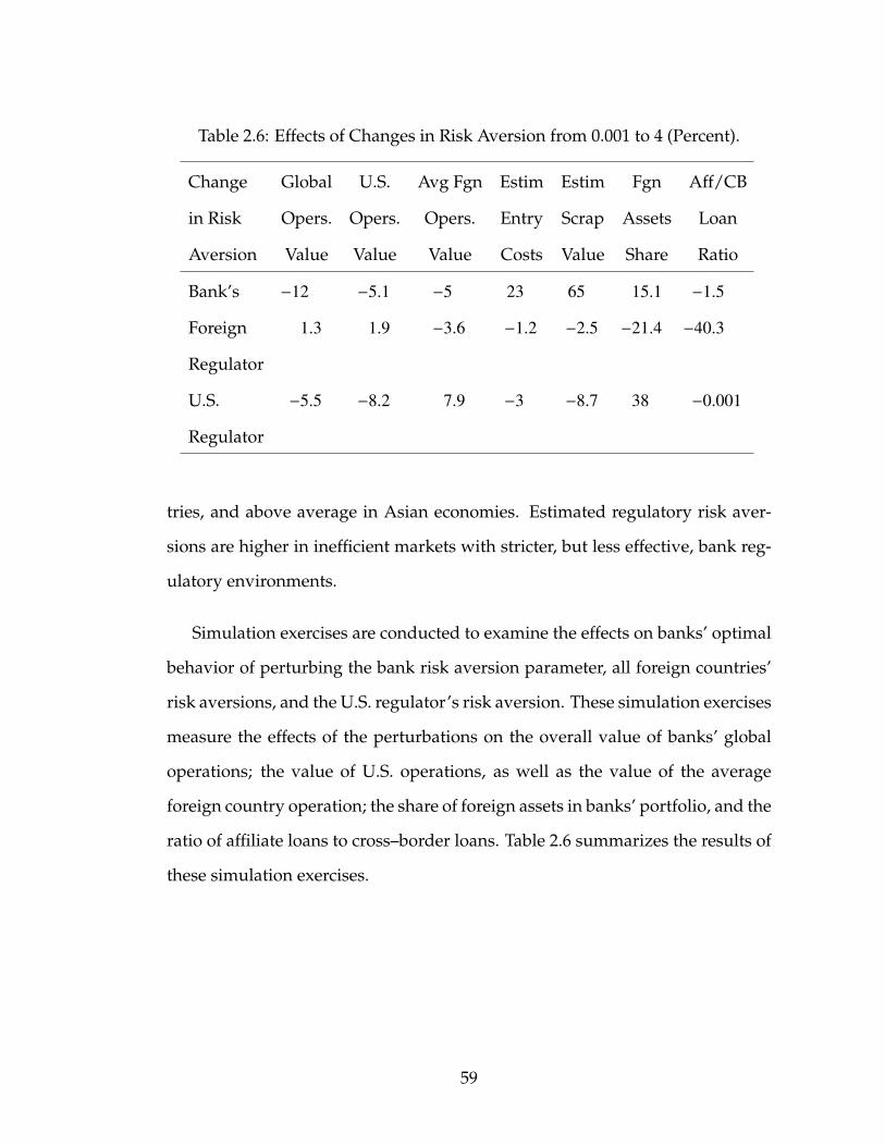
Table 2.6: Effects of Changes in Risk Aversion from 0.001 to 4 (Percent).

Change Global U.S. Avg Fgn Estim Estim Fgn Aff/CB

in Risk Opers. Opers. Opers. Entry Scrap Assets Loan

Aversion Value Value Value Costs Value Share Ratio

Bank’s −12 −5.1 −5 23 65 15.1 −1.5

Foreign 1.3 1.9 −3.6 −1.2 −2.5 −21.4 −40.3

Regulator

U.S. −5.5 −8.2 7.9 −3 −8.7 38 −0.001

Regulator

tries, and above average in Asian economies. Estimated regulatory risk aver-

sions are higher in inefficient markets with stricter, but less effective, bank reg-

ulatory environments.

Simulation exercises are conducted to examine the effects on banks’ optimal

behavior of perturbing the bank risk aversion parameter, all foreign countries’

risk aversions, and the U.S. regulator’s risk aversion. These simulation exercises

measure the effects of the perturbations on the overall value of banks’ global

operations; the value of U.S. operations, as well as the value of the average

foreign country operation; the share of foreign assets in banks’ portfolio, and the

ratio of affiliate loans to cross–border loans. Table 2.6 summarizes the results of

these simulation exercises.

59

CHAPTER 3

BRANCH NETWORK AND INTEREST RATE CHOICES OF HUNGARIAN

COMMERCIAL BANKS

3.1 Introduction

Numerous studies and bank surveys (Bancography, 2003; Spieker, 2004) show

that branch networks are an important strategic tool of commercial banks, in ad-

dition to the choices of interest rates. While building new branches is a power-

ful method of expanding market share, doing so is also very expensive. Surveys

measured the fixed setup cost of a new branch to range from 1 million U.S. Dol-

lars (Sheffield, 2006) to upward of 2 million U.S. Dollars (Spieker, 2004) in the

U.S., which does not even include associated operating expenditures (Bancog-

raphy, 2003). 1. In light of the non–trivial benefits of branch network expansion,

the purpose of this chapter is to examine imperfectly competitive Hungarian

commercial banks’s strategic choices of interest rates and branch network size

in a dynamic setting. The chapter formulates a comprehensive model of bank

behavior that captures branch network competition. Using bank–level Hun-

garian commercial banking data, the determinants of interest rate and branch

network size choices, as well as the fixed branch setup costs and scrap values

are estimated based on the modeling framework.

Branch network decisions are very closely tied to client location and socioe-

conomic status. Looking at the U.S. commercial banking market, surveys of the

Federal Reserve Board suggest that the single most important factor influencing

1In the case of U.S. commercial banks, it has been documented that average total costs actu-ally increase with branch network size (Spieker, 2004)

60

customers’ choice of banks is the location of bank’s branches (Governor Mark

W. Olson, 2004). Furthermore, MarkeTech International assessed that traits re-

lated to location may account for 45 to 55 percent of deposit formation (Hopson

and Rymers, 2003). Banks indeed take account of these factors in their branch-

ing decisions: per capita income and population density have been shown to be

significant drivers of branch network expansion. These observations on bank

and client behavior are the motivation behind this chapter’s modeling of com-

mercial bank branch network size choice as a game of spatial competition.

This chapter presents a dynamic Salop–style spatial competition model of

profit maximizing commercial banks. Banks participate in retail and corpo-

rate banking markets. In the retail banking market, banks make loans in a

variety of currencies, and compete in lending, mortgage and deposit rates, as

well as their branch network size. Banks derive market power from the loca-

tion of their branches, which they can influence by expanding or contracting

their branch network. The corporate banking market is modeled as perfectly

competitive, motivated by the discussions of Hungarian commercial banking in

Molnar, Horvath, and Nagy (2007) and More and Nagy (2004). Therefore, banks

take the corporate lending rates of all currencies as given.

Banks’ dynamic profit maximization problem consists of two types of deci-

sions. On one hand, banks make interest rate choices period by period. Interest

rate choices only influence current profits and are therefore static.2 On the other

hand, banks choose the size of their branch network. Branch setup and closing

decisions have–long term consequences, as the resulting branch network size

will impact market share and interest rate choices for periods to come. In this

2That is, banks reassess the interest rates they charge on loans and pay on deposits eachperiod.

61

chapter’s modeling of branch opening and closing decisions, banks take these

long–term consequences into account.

A version of the Bajari, Benkard, and Levin (2007) simulation–based estima-

tion method is fitted to the framework of the theoretical model. Banks’ opti-

mal choices are estimated in two stages. The first stage examines the impact

of current state variables (such as competitors’ branch network size, consumer

income, etc.) on banks’ choices of interest rates. This stage also yields esti-

mates of the determinants of banks’ choices of how many new branches to open

or close (constituting the transition probabilities for branch network size). Re-

sults show that banks charge a premium for greater branch network size in their

lending rates, and offer lower deposit rates accordingly. Furthermore, greater

branch network size of competitors induces banks to ask lower rates on loans,

and offer higher deposit rates. A similar competitive pattern is observed in the

branch network expansion and contraction choices: more branches of competi-

tors make banks more likely to expand. Furthermore, banks with bigger branch

networks are less likely to add new branches.

The second stage of the estimation uses the first–stage policy function esti-

mates to construct banks’ discounted expected sum of profits via forward sim-

ulation. Using the structure fitted to bank behavior, the values of numerous

alternate policy paths are simulated. Estimates of branch setup costs and scrap

values are then chosen to ensure that banks’ observed (optimal) actions yield

the highest bank value. Monthly estimates of branch setup costs show that with

an average cost of 148.81 million HUF (approximately 0.75 million USD), set-

ting up branches is considerably cheaper in Hungary than the U.S.3. With a

mean of 109.48 million HUF, scrap values are approximately 75 percent of setup

3Much of this difference is likely be explained by deviations from price parity

62

costs. Setup costs and scrap values are very strongly positively correlated. Fur-

thermore, they move closely with producer price indices capturing the cost of

manufacturing and construction. Various simulation exercises are presented

following the estimation, confirming the important role of branch network com-

petition in bank behavior.

The chapter proceeds as follows. Subsection 3.1.1 provides an overview of

Hungarian commercial banks’ behavior during the sample period of January

2004 to November 2007. Section 3.2 motivates the modeling framework in the

context of the related literature. Section 3.3 presents the model and character-

izes banks’ optimal behavior. Section 3.4 covers the estimation method and de-

scribes the data. Section 3.5 presents and discusses the estimation results, and

Section 3.6 describes the simulation exercises. Section 3.7 summarizes and con-

cludes the chapter.

3.1.1 Overview of the Hungarian Commercial Banking Market

The time period under examination in this paper is January 2004 to November

2007. During this time, the Hungarian retail banking sector is characterized

by a high degree of market power, and active branch network expansion and

contraction. The overview in this subsection focuses on two strategic tools of

competition: choices of interest rates and branch network size.

An interesting and unique characteristic of the former Communist Central

and Eastern European economies is the high share of foreign currency lend-

ing and deposit–taking relative to the local currency. During the period un-

der examination, an average of 70 percent of Hungarian bank lending took

63

place in foreign currencies, mostly in Euros (EUR), the Swiss Franc (CHF) and

the Japanese Yen (YEN). Various foreign currencies appear within sub–types of

loans (mortgages, retail, corporate), i.e. there is no specialization of loan types

by currency.

Aug2003 Feb2004 Sep2004 Mar2005 Oct2005 May2006 Nov2006 Jun2007 Dec20070

5

10

15

20

25

30

Time Period

Ret

ail L

endi

ng R

ates

by

Cur

renc

y

HUF Lending Rates EUR Lending Rates CHF Lending Rates

Figure 3.1: Average Retail Loan Rates by Currency Over Time.

Aug2003 Feb2004 Sep2004 Mar2005 Oct2005 May2006 Nov2006 Jun2007 Dec20070

5

10

15

20

25

30

Time Period

Dep

osit

Rat

es b

y C

urre

ncy

HUF Deposit RateEUR Deposit Rate

Figure 3.2: Average Retail Deposit Rates by Currency Over Time.

64

Aug2003 Feb2004 Sep2004 Mar2005 Oct2005 May2006 Nov2006 Jun2007 Dec20070

5

10

15

20

25

30

Time Period

Mor

tgag

e R

ates

by

Cur

renc

y

HUF Mortgage RatesEUR Mortgage RatesCHF Mortgage Rates

Figure 3.3: Average Mortgage Rates by Currency Over Time.

Aug2003 Feb2004 Sep2004 Mar2005 Oct2005 May2006 Nov2006 Jun2007 Dec20070

5

10

15

20

25

30

Time Period

Cor

pora

te L

endi

ng R

ates

by

Cur

renc

y

HUF Firm Lending RatesEUR Firm Lending Rates

Figure 3.4: Average Corporate Lending Rates by Currency Over Time.

It is interesting to explore the reasons underlying the use of multiple curren-

cies by banks: Ize and Yeyati (2003) show that risk averse banks are more prone

to foreign currency holdings in the presence of lower exchange rate volatility

and high price volatility. Pellenyi and Bilek (2009) argue that both these factors

were present in Hungary during the 2004–2007 period: inflation was relatively

high compared to the EUR and CHF. At the same time, the Gyurcsany Admin-

65

istration promised to reduce exchange rate volatility by keeping the HUF fluc-

tuations against the EUR within a 15 percent band (according to ERM-II). This

latter action also contributed to the fact that consumers treated loans of various

currencies as near perfect substitutes, vastly underestimating currency risk in

pursuit of the significantly lower interest rates on foreign currency loans.4

Figures 3.1 and 3.3 and 3.4 show that the lending rates on different currency

denominations vary widely. Most notable is the large spread between the retail

lending rates on EUR and CHF loans, compared to the the HUF rate. Adjust-

ing for expectations in currency appreciation (as well as inflation) does not ex-

plain away the large observed interest rate spreads between HUF and foreign

currency–denominated loans.5 The interest rate gap that remains between HUF

and foreign currency loans after adjustments is large at around 10 percent. Per-

sistent deviations from UIP have been well documented in the literature (Froot

and Thaler, 1990). What might explain the empirical failure of UIP in the Hun-

garian case?

There is a clear and solid explanation for the low cost of foreign currency

borrowing in Hungary. Basso, Calvo-Gonzales, and Jurgilas (2007) argue that

banks which are headquartered abroad (characterizing the majority of Hungar-

ian commercial banks) have easy access to foreign currency, at a low cost.6 In

the presence of monopolistic competition, they can use this advantage to com-

pete for consumers via lower rates on foreign currency loans. Furthermore, it

4Pellenyi and Bilek (2009) also present evidence that socioeconomic characteristics (such aseducation, income, etc.) fail to explain borrowers’ choice of currency denominations.

5While Uncovered Interest Parity (UIP) does not explain the difference between HUF andforeign currency lending rates — as shown in Figure B.1 — it is in fact able to account fordifferences between observed EUR and CHF loan rates. It also explains differences in HUF andEUR deposit rates as shown by Figure B.2.

6Most foreign banks operating in Hungary are from Euro–zone countries. Therefore, theempirical fact that appreciation and inflation–adjusted EUR rates are consistently the lowest isin line with this argument on lower cost of foreign currency access.

66

has been argued that the very high cost of HUF borrowing is due to the uncer-

tainty banks face in light of the unpredictable and imprudent fiscal policy of the

Hungarian government (Ewing, May 6 2010). The time period under consider-

ation between 2004 and 2007 was indeed characterized by a lot of uncertainty

about fiscal policy, culminating in Prime Minister Gyurcsany’s admission (on

September 18, 2006) of having lied about fiscal actions and outcomes for several

consecutive years (Condon, September 19 2006).

In light of the apparent gap between HUF and foreign currency borrow-

ing rates, it is important to address the issue of arbitrage. For banks, the arbi-

trage opportunity would be to borrow from their Euro–zone parents at a low

rate, change foreign currency into HUF, and make HUF loans at the higher rate.

However, the lack of demand for loans at high rates greatly limits this opportu-

nity. From consumers’ perspective, the arbitrage opportunity would be to take

out EUR and CHF loans at low rates, then re–lend the money at the higher rates

after conversion into HUF. However, this opportunity is again limited by the ap-

parent and persistent lack of demand for HUF loans at the high rates (Holland,

Cochrane, and Penz, October 30 2008).

An important goal of this chapter is to address the role of branch networks

in competition. Branch network size is an important source of market power

in Hungary. According to Cottarelli (1998), ”[the persistent market power of

commercial banks is] largely reflecting their continued branch monopoly in re-

gions of the country. The factor behind the continued dominance of these banks

is the relatively high cost of establishing a branch network”. It is indeed proof

of the continued use of branch networks as a strategic tool that the time pe-

riod under examination is very active in terms of branch network expansion

67

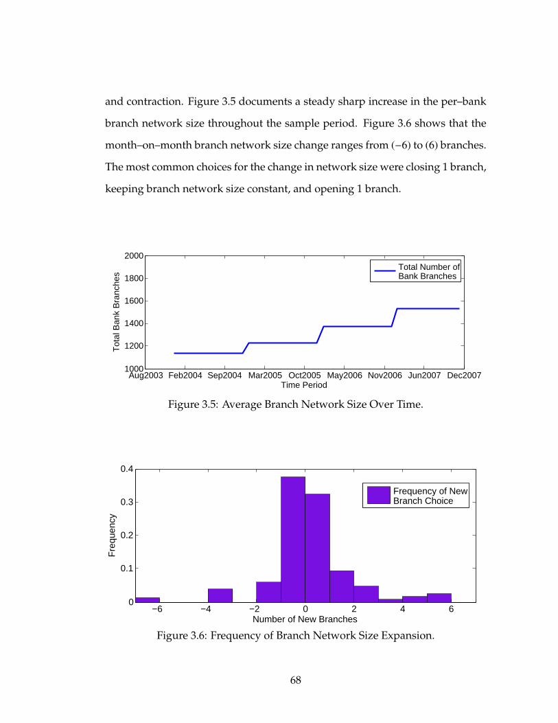
and contraction. Figure 3.5 documents a steady sharp increase in the per–bank

branch network size throughout the sample period. Figure 3.6 shows that the

month–on–month branch network size change ranges from (−6) to (6) branches.

The most common choices for the change in network size were closing 1 branch,

keeping branch network size constant, and opening 1 branch.

Aug2003 Feb2004 Sep2004 Mar2005 Oct2005 May2006 Nov2006 Jun2007 Dec20071000

1200

1400

1600

1800

2000

Time Period

Tot

al B

ank

Bra

nche

s

Total Number ofBank Branches

Figure 3.5: Average Branch Network Size Over Time.

−6 −4 −2 0 2 4 60

0.1

0.2

0.3

0.4

Number of New Branches

Fre

quen

cy

Frequency of NewBranch Choice

Figure 3.6: Frequency of Branch Network Size Expansion.

68

3.2 Motivation and Related Literature

This section gives summaries of the three strands of relevant literature. These

strands are: (1) modeling imperfect and spatial competition in commercial bank-

ing; (2) dynamic estimation techniques for models of imperfect competition,

and (3) evolution of Hungarian commercial banking.

3.2.1 Commercial Bank Competition

There have been numerous, mostly empirical papers, addressing spatial (branch

network) competition in commercial banking markets. Most of the previous

studies have focused on only one of the areas of deposit rate, lending rate or

branch network competition. As an early example, Barros (1999) develops a

spatial competition model to explain price differences across banks in the de-

posit market. His model separates two sources of market power: collusion in

banking services, and location (taking branch networks as given). The paper

examines whether banks’ profitability is a result of conduct or market structure

(location). He finds that location–based market power is the more important

explanation for high margins in deposits. The applicability of Barros’ work to

the current framework is limited in that (1) he takes loan markets and branch

networks as given — examining deposit rates as the only strategic tool, and (2)

he abstracts away from any dynamic considerations.

Dell’Ariccia (2001) paints a more complete picture of strategic bank behav-

ior by presenting a multi–period model of spatial competition, where banks’

entry/exit decisions are endogenously determined. The paper shows that un-

69

der asymmetric information and learning by lending, in equilibrium there is a

finite number of competitors even in the absence of exogenous fixed costs. Even

though the theoretical model (a multi–period extension of the Salop spatial com-

petition model) is similar to the one presented in this chapter, Dell’Ariccia ex-

cludes branch banking as a strategic decision (the strategic choice of banks is

whether to exist or not).

The work of Calem and Nakamura (1998) is one step closer to the frame-

work of this chapter in that they explicitly include branch network competition.

They build a model to show that branch banking broadens the geographic scope

of competition among banks, and that banking services at peripheral locations

will be priced more competitively when those locales are served by branch net-

works. Their theoretical model contains a central location with multiple bank-

ing outlets, and outlying locations with few banking outlets. Calem and Naka-

mura find that branching restrictions are associated with larger price differen-

tials across banks. While their paper depicts branch banking, their main focus

is to model a Bertrand pricing game between two banks that are competitors at

the central location, but also have outlying branches.

Another step closer to the formulation of this chapter is Chiappori, Perez-

Castrillo, and Verdier (1995). They analyze a spatial competition model of the

banking sector, where banks offer loan and deposit services — though in a static

setting. The goal of their paper is to investigate the consequences of the regu-

lation of rates paid on deposits. The authors find that regulation first increases

network size beyond social optimum, and in the long run result in lower equi-

librium credit rates because of increased competition. They also show that reg-

ulation leads to tied services — as a result, an upper limit on deposit rates also

70

restricts lending rates. They consider a one–period imperfect price competition

model. The paper also incorporates spatial competition in the Salop framework.

The applicability of their approach to this chapter is limited in that the authors

exclude multi–branch banking by considering each branch to be an independent

entity.

Kim and Vale (2001) build a bank branching model, where they consider the

role of the size of the branch network in the provision of loans. The authors

estimate a model of branching decisions where banks explicitly take account of

both their own existing network and their expectation of rivals’ choices. The

paper tests whether there exist external informational spill–overs among banks

due to branch network proliferation. They want to see whether branch net-

works have a market size effect, or only a market share effect. The paper sets

up a non–price oligopolistic model of bank behavior in the loan market. The

authors derive and estimate a simultaneous equations system of bank–level op-

timization rules for branching choice and loan equations. The predictions of

the model are tested on Norwegian bank–level panel data. The paper’s multi–

period spatial competition model is relevant for this chapter, since it explicitly

incorporates bank branching choices. However, in their model there is no price

(interest rate) competition — banks treat loan quantities as their choice variable

instead.

Estrada and Rozo’s (2006) model incorporates competition in interest rates

as well. They present a multi–market spatial competition oligopoly structure

for the Colombian deposit market. In their model, banks use price and non–

price strategies to compete in two periods. In the first period, banks choose

the optimal loan and deposit rates for the whole country, according to Bertrand

71

competition. In the second period, banks select the number of branches they

plan to open in each region, given the optimal interest rates. While the strategic

variables and the multi–period setup is relevant, their two–step optimization

approach diverges from this chapter’s goal. This is because the current chapter

aims to model banks’ lending and deposit rate, as well as bank network size

choices simultaneously.

The modeling approach presented in this chapter is in agreement with that of

Cerasi, Chizzolini, and Ivaldi (2002), who argue that branch network and price

competition are closely tied together, and must be simultaneously modeled.

They do this using a static non–cooperative two–stage game, where branching

decisions are taken in the first stage, and monopolistically competitive interest

rates are set in the second stage. The authors derive structural equations in or-

der to measure branching costs and degree of competition in banking services,

and fit the model’s equations to bank–level European panel data.

Closest to this chapter is the work of Kim, Lozano-Vivas, and Morales (2007),

who present a multi–strategic, multi–market and multi–output oligopolistic spa-

tial model of a monopolistically competitive banking sector. In their model,

banks take explicit account of the impact of their strategies on their existing

branch network and market share, as well as the reaction of their competitors.

The three strategic variables of each bank are: deposit interest rates, loan inter-

est rates and the number of branches in a given region. Kim, Vivas and Morales

present a static model, whose parameters are estimated using Spanish data. This

chapter takes a similar modeling framework and extends it to a more realistic

dynamic setting.

A closely related paper by Berger and Mester (2003) examines the relation-

72

ship between commercial bank efficiency and branch network size. They find

that greater branch network size does not provide cost efficiencies — but there

are indeed revenue improvements. The authors explain banks’ continued drive

to expand their branch network size and improve services by the assertion that

the corresponding growth in revenues outpaces cost increases.

An important part of this chapter’s analysis is to account for how consumers

respond to changes in the attributes of banking services (albeit in a spatial com-

petition framework). This approach is motivated by Dick (2007), who estimates

the demand for deposit services in the U.S. commercial banking industry. Her

goal is to assess the effect on consumers of the significant changes in banking

services throughout the 1990s. Dick’s model accommodates the various changes

that have taken place in banking markets, as well as the elimination of branch-

ing restrictions on U.S. banks. The author estimates a multinomial discrete

choice nested logit model of demand. This is a structural model which incor-

porates product differentiation. The results show that consumers respond to

various bank attributes, beyond prices. The results also suggest that consumers

have benefited from nationwide branching in the United States.

3.2.2 Estimation Method

The main contribution of this chapter compared to previous literature is the pre-

sentation of spatial bank competition in a dynamic framework. Taking account

of dynamics is especially important when looking at branch network competi-

tion, where branch building and closing decisions have consequences that last

well beyond a single period. However, solving a full–fledged dynamic opti-

73

mization problem has a very high computational cost. The problem is made

tractable by formulating a version of the Bajari, Benkard, and Levin (2007) two–

step estimation method (motivated by Hotz and Miller (1993)) for the current

framework.

The first stage of the two–step estimation consists of a reduced–form regres-

sion of banks’ policy functions on all the current state variables. Using these

estimates, it is possible to get a form of banks’ discounted sum of expected prof-

its as functions of the state variables and the model’s structural parameters only.

Furthermore, data can be used to estimate the transition probabilities of all the

relevant state variables. The second stage consists of forward simulation of the

values of bank’s optimal choices. Best estimates of the structural parameters

are then chosen to ensure the optimality of observed actions compared to any

other sub–optimal policy paths. Further relevant papers — discussing estima-

tion methods which avoid solving the full–blown dynamic optimization prob-

lem — are Ericson and Pakes (1995), Berry, Levinsohn, and Pakes (1995), Olley

and Pakes (1996) and Pakes, Ostrovsky, and Berry. (2007).

3.2.3 Evolution of Hungarian Commercial Banking

There have been numerous papers examining the conditions of the Hungar-

ian commercial retail banking market starting with the first years of privati-

zation in the early 1990s (Abel and Bonin, 2000; Abel and Siklos, 2004; Kiraly

and Varhegyi, 2004; Majnoni, Shankar, and Varhegyi, 2003). Notably, Varhegyi

(2004) describes the competitive evolution of the Hungarian banking sector. She

examines bank competition in Hungary using a structural approach. This ap-

74

proach assumes that the best way to influence competition is by affecting the

market structure. The study first examines bank competition in Hungary since

1990, and then uses behavioral models to describe bank competition in the pe-

riod 1995–2002. The paper argues that during this period, banks had a price–

setting role in loan markets, and a price–accepting role in deposit markets. The

author uses various empirical I.O. models to test market structure and market

power. The modeling formulation of this chapter is partly motivated by the fol-

lowing findings of Varhegyi (2004): (1) while the corporate loan market is com-

petitive, the retail market is still characterized by considerable market power of

banks, and (2) price competition is the best description of strategic choices in

the Hungarian banking market — while collusion can be ruled out.

In a related paper, More and Nagy (2004) investigate the degree of bank com-

petition in Hungary in various sub–markets. The authors conjecture that there

is a high degree of market power in consumer lending, and that competitive

pricing prevails in the corporate lending market (in line with Varhegyi (2004)).

More and Nagy (2004) use a non–structural model of competition to test their

hypotheses of competition, using bank–level panel data. After estimating con-

jectural variation for each sub–market, they show that the degree of competi-

tion in both the loan and deposit markets falls between perfect competition and

the Cournot equilibrium. The consumer credit sub–market, however, is charac-

terized by a much lower degree of competition: between Cournot equilibrium

and perfect collusion. Low level of competition and inelastic demand allows

banks to receive large oligopolistic rents in the consumer credit sub–market. Es-

timating the loss of consumer surplus resulting from imperfect competition, the

authors find these losses to be small.

75

The model of this chapter is informed by Molnar, Horvath, and Nagy (2007),

who build a structural model of the Hungarian retail banking industry. In this

static model, the authors estimate residual demand and supply functions of

household loan and deposit services. For the supply side, the authors consider

two models of the banking industry: a static, differentiated–product Nash–

Bertrand oligopoly and a cartel. For each supply model, the pricing decisions of

the bank depend on the individual bank–level demands. The authors estimate a

discrete choice multinomial logit model of demand for consumers’ loan demand

and deposit services. The results show that the observed price–cost margins are

very high for overdrafts, higher purchase loans, personal loans and demand

deposits, and lower for short–term and long–term deposits. In order to iden-

tify the structure of competition, the authors compare the estimated price–cost

margins implied by the Nash–Bertrand and cartel models to the observed val-

ues. The results suggest that in the overdraft, hire purchase loan, personal loan,

demand deposit, and short–term deposit markets, the degree of competition

is low. Long-term deposit markets can be characterized as fairly competitive.

When the authors control for consumer default risks and inflation, the observed

margins are even closer to competitive values.

3.3 Model

This section describes the theoretical modeling framework. The economy con-

sists of households, firms and commercial banks. There is a large number of

utility–maximizing households. The corporate sector consists of a fixed number

of profit–maximizing firms f = 1 . . . F. There is a total number of T periods, with

t indexing the individual period. The time subscript is suppressed throughout

76

the description of the model. There are a total of J commercial banks in the

economy, with j = 1 . . . J indexing the individual bank. Commercial banks pro-

vide deposit and loan services to retail customers, and loan services to corporate

customers. Banks’ goal is to maximize the discounted sum of expected profits

over time. They do so by choosing lending rates, deposit rates and their branch

network size in the retail sector. Banks choose their optimal lending rates in the

corporate sector (where there is no spatial competition, and network size plays

no role).

The economy consists of a single location, which has a circular shape in ac-

cordance with the Salop spatial competition model as described in Salop (1979)

and Freixas and Rochet (2008). The circular economy has circumference A. Each

bank j has one headquarter, and a number n of bank branches, denoted by n j.

Then the total number of branches in the economy is N =∑

j n j. Bank branches

are uniformly distributed along the Salop circle, so that the distance between

each branch is AN . Households are also uniformly distributed along the Salop

circle, with a total mass of A. As banks increase their branch network size, N

changes over time. However, A changes at the same rate as N, so that the ra-

tio A/N (and hence the location of each existing branch) is independent of new

branching decisions. Figure 3.7 describes the locational structure of the model.

3.3.1 Retail Sector — Households

Households live for two periods, and consume the single consumption good c

in each period. Households form overlapping generations, so that some house-

holds are in their first period of life, while others are in their second (last) period

77

Bank Headquarters

Uniformly distributed Bank Branches Distance between

branches is A/N

Branch Y

Branch Z

Distance x

Location of Marginal

Household Client

Indifferent between

Branches Y and Z

Distance A/N-x

Figure 3.7: Illustration of Model Structure.

of life in each period t. Given their income I, each household’s goal is to choose

consumption ct so as to maximize the sum of its discounted expected utility

over the two periods of its lifetime. Households are identical except for their

discount factor βh, which defines each household’s ‘type’. The discount factor

is known and is drawn from a uniform distribution U[0, 1]. This distribution is

constant over time, and the βh draws are independent across periods.

Households can save (and deposit at the bank) some of their income in the

first period of their life, that is, when they are young. A negative saving sh < 0

implies borrowing. Households deposit their saving and obtain their borrowing

at the nearest bank branch along the circle. The nearest branch charges rate rhl

on loans and pays rate rhd on deposits.

The retail banking market (both lending and deposit–taking) is monopolisti-

cally competitive. This is because households are constrained by their location,

and can only choose between the two nearest branches. This serves as a source

of market power for banks. Each household takes(I; βh; rh

d; rhl

)as given. Let x

78

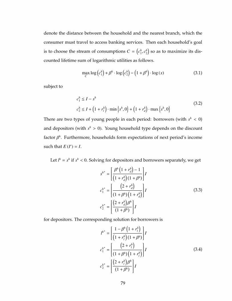
denote the distance between the household and the nearest branch, which the

consumer must travel to access banking services. Then each household’s goal

is to choose the stream of consumptions C =(ch

1, ch2

)so as to maximize its dis-

counted lifetime sum of logarithmic utilities as follows.

maxC

log(ch

1

)+ βh · log

(ch

2

)−

(1 + βh

)· log (x) (3.1)

subject to

ch1 ≤ I − sh

ch2 ≤ I +

(1 + rh

l

)·min

sh, 0

+

(1 + rh

d

)·max

sh, 0

(3.2)

There are two types of young people in each period: borrowers (with sh < 0)

and depositors (with sh > 0). Young household type depends on the discount

factor βh. Furthermore, households form expectations of next period’s income

such that E (I′) = I.

Let lh = sh if sh < 0. Solving for depositors and borrowers separately, we get

sh∗ =

βh(1 + rh

d

)− 1(

1 + rhd

) (1 + βh)

I

ch1∗

=

(2 + rh

d

)(1 + βh) (1 + rh

d

) I

ch2∗

=

(2 + rh

d

)βh(

1 + βh) I

(3.3)

for depositors. The corresponding solution for borrowers is

lh∗ =

1 − βh(1 + rh

l

)(1 + rh

l

) (1 + βh)

I

ch1∗

=

(2 + rh

l

)(1 + βh) (1 + rh

l

) I

ch2∗

=

(2 + rh

l

)βh(

1 + βh) I

(3.4)

79

It follows that the effect of βh on whether the household is a depositor or

borrower is as follows:

Depositor if1

1 + rhd

< βh

No banking if1

1 + rhl

< βh <1

1 + rhd

Borrower if βh <1

1 + rhl

(3.5)

Given the known uniform distribution of βh and the total mass of consumers A,

we can integrate over the ranges defined in (3.5) to get the approximate market

supply of deposits and market demand for loans as follows.

Deposit Supply:

Dh =

∫ 1

(1+rhd)−1

(sh

)∗dβh · A =

(3.2rh

d + 0.4 + rh2d

)· I · A

Loan Demand:

Lh =

∫ (1+rhl )−1

0

(lh)∗

dβh · A =(1 − 1.5rh

l − rh2l

)· I · A

(3.6)

Banks observe the market supply of deposits and the market demand for loans.

Substitution of the optimal solutions from Equations (3.3) and (3.4) yields the

young household’s lifetime indirect utility Vh. Letting subscript m = (d, l) for

deposits and loans, this indirect utility is given by

Vh(βh, I, x, rh

m

)= u

(ch

1

)∗+ βh · u

(ch

2

)∗−

(1 + βh

)· log (x) =

log

(2 + rh

m

)· I(

1 + βh) (1 + rhm) + βh · log

βh ·

(2 + rh

m

)· I

1 + βh

− (1 + βh

)· log (x) (3.7)

Given that households are uniformly distributed along the Salop circle, they

can choose to bank at either of the two nearest bank branches, depending on the

offered interest rates rhm and the distance x. Let j and j + 1 index two branches

owned by bank j and j + 1, respectively. The location of the marginal household

80

is characterized by the critical value of x, denoted by x, such that the household

is indifferent between going to branch j and branch j + 1. Let rhj and rh

j+1 denote

the rates offered at branches j and j + 1, respectively. Using a first–order Taylor

expansion and (3.7), the approximate location of the marginal household is7

x =A ·

(2 +

(rh

j − rhj+1

)·(βh ·

(1 + rh

j

)− 1

))4N ·

(1 + βh) (3.8)

From (3.8) it follows that a higher x means more customers for branch j. There-

fore, (3.8) implies that branch j’s borrower customer base shrinks with higher

lending rates, and its depositor base increases in higher rates. Similarly, higher

lending rates of competitors increase branch j’s client base, while higher deposit

rates of competitors mean fewer depositors at branch j8. Furthermore, rhj = rh

j+1

implies that the marginal client is halfway between the two nearest branches.

Banks observe the location of the marginal household, and take x into account

in their deposit/lending rate and branch network size decisions. In the follow-

ing analysis, the values of β are fixed such that βh = 0 for those who borrow, and

βh = 1 for depositors.

3.3.2 Firms

There are F firms in the economy, with subscript f denoting the individual firm.

Firms are owned by shareholders, who provide starting capital b in each period.

Shareholders’ goal is to maximize profits over the course of two periods. Profits

are distributed to shareholders at the end of the second period. Each firm pro-

duces a single good yt that is identical across all firms. Let superscript c denote

7This critical value x is obtained by solving V(βh, I, x, rh

j

)= V

(βh, I,

(AN − x

), rh

j+1

).

8This follows directly from the characterization described in (3.5).

81

corporate. Capital K =(kc

1; kc2

)is the only input in the production of the iden-

tical good. The production function is concave and given by y = f (kc). The

production technology is identical across all firms and over time.

Banks lend to firms in perfectly competitive loan markets. Each firm can obtain

corporate loan lc from banks at the perfectly competitive corporate lending rate

rcl . Corporate loan lc borrowed in the first period must be repaid in the second

period. Firms sell their output to households for consumption. Households

pay a price of one (unity) for the output in both periods of the firm’s life. Let βc

denote the firm’s known discount factor, whose uniform distribution U [0, 1] is

constant over time (with the βc draws also independent over time). Then firm

f ’s two–period profit-maximization problem is to choose K =(kc

1; kc2

)so as to

maxK

√kc

1 + βc ·

√kc

2

subject tokc

1 ≤ b + lc

kc2 ≤ b −

(1 + rc

l)· lc

(3.9)

The corresponding optimal solutions are

(kc

1)∗

=

(2 + rc

l

)· b(

1 + rcl

) (1 + βc2

(1 + rc

l

))(kc

2)∗

=βc2

(1 + rc

l

) (2 + rc

l

)· b

1 + βc2(1 + rc

l

)l∗ct =

(1 − βc2

(1 + rc

l

)2)· b(

1 + rcl

) (1 + βc2

(1 + rc

l

))(3.10)

It follows that each firm borrows a non–negative amount only if its discount

factor βc is sufficiently low, i.e. if βc ≤(1 + rc

l

)−1. Since there are F identical firms

82

in the economy, firms’ market demand function for bank loans is given by

(Lc)∗ =

(1 − βc2

(1 + rc

l

))· F · b(

1 + rcl

) (1 + βc2

(1 + rc

l

)) (3.11)

Each bank observes this market demand function for loans.

3.3.3 Banks

Bank Services to Households

Each bank j provides lending and deposit services to households after choosing

its optimal retail lending rate(rh

l j

)∗, retail deposit rate

(rh

d j

)∗and branch network

size(n j

)∗. Recall that each bank can operate multiple branches. Suppose bank

j operates the j’th branch. The quantities of deposits supplied and loans de-

manded depend on whether the neighboring branches — denoted by j − 1 and

j + 1 — belong the bank j or not. Given the characterization in (3.8) of the

location of the marginal household, the expected volume of loans and deposits

attracted by bank j is

E(Lh

j

)= n j ·

Lh

4·

AN·

[Prob ( j − 1 = j) · Prob ( j + 1 = j) · (4)

+ Prob ( j − 1 , j) · Prob ( j + 1 , j) ·(4 + rh

l j+1 + rhl j−1 − 2rh

l j

)+ Prob ( j − 1 = j) · Prob ( j + 1 , j) ·

(4 + 2

(2 + rh

l j+1 − rhl j

))](3.12)

In (3.12), the first line within the curly brackets shows the expected branch–

specific loan demand if both neighboring branches belong to bank j. The second

line shows the expected demand if none of the neighboring branches belong

to bank j. The last line shows the expected branch–level demand if only one

83

of the neighboring branches belongs to bank j. The per–branch expected loan

demand is then multiplied by the number of branches bank j owns. The similar

expression for the quantity of deposits supplied that bank j expects to attract is:

E(Dh

j

)= n j ·

A8N·

Dh

A·

[Prob ( j − 1 = j) · Prob ( j + 1 = j) · (4)

+ Prob ( j − 1 , j) · Prob ( j + 1 , j) ·(4 + rh

d j ·(2rh

d j − rhd j+1 − rh

d j−1

))+ Prob ( j − 1 = j) · Prob ( j + 1 , j) ·

(8 + 2rh

d j ·(rh

d j−hd j+1

))](3.13)

Note that Equations (3.12) and (3.13) are constant in the term AN . This implies that

new branches bring new customers, and the location of each existing branch

is independent of new branching decisions. A further implication is that new

branches do not cause consumers to regroup. Therefore, for given interest rates

there are two ways branch network size n j impacts the expected loan and de-

posit volumes of bank j. First, adding a new branch expands the loan and de-

posit volumes by the per–branch amounts shown in (3.12) and (3.13) in curly

brackets. Second, n j affects the probabilities that the neighboring branches also

belong to bank j. The following subsections describe banks’ optimal choices of

the interest rates and branch network size.

3.3.4 Price Competition

Banks choose their interest rates period by period, in an imperfect competition

setting. The interest rate choices are static because profits are redistributed to

bank shareholders at the end of each period. Therefore, chosen interest rates in-

fluence current profits, but have no impact on future profits. Let Ψ =(ch

l ; chd; cc

l

)denote the proportional costs of household lending, deposit taking and corpo-

rate lending, respectively. Furthermore, φ is the required reserve ratio, r de-

84

notes the interest paid on interbank loans and cn j is the per–branch operational

cost. In price competition, each bank’s goal is to choose the optimal values of

R∗j =(rh∗

l j ; rh∗d j; rc∗

l j

)so as to maximize the price–relevant part of its profit function

in each period, taking its network size n j as given.

maxR j

E(π j

)=

(rh

l j − r − chl j

)· E

(Lh

j

)+

(r · (1 − φ) − rh

d j − chd j

)· E

(Dh

j

)+

(rc

l j − r − ccl j

)· Lc

j − cn j · n j (3.14)

Since the corporate sector is monopolistically competitive, the lending rate

there is equal to the marginal cost of lending. Furthermore, the corporate market

is equally divided among all banks lending to firms. The following first–order

optimality conditions characterize the optimal choices of retail lending, retail

deposit and corporate lending rates, respectively.

E(Lh

j

)+

(rh

l j − r − chl j

)·∂E

(Lh

j

)∂rh

l j

= 0 (3.15)

−E(Dh

j

)+

(r · (1 − φ) − rh

d j − chd j

)·∂E

(Dh

j

)∂rh

d j

= 0 (3.16)

rcl j = cc

l j + r (3.17)

In this model there are multiple equilibria, so that the equilibrium charac-

terized by (3.15) through (3.17) is not unique. In what follows, the equilibrium

yielding the highest price (interest rate) is selected, in order to underline the role

of market power and deviation from perfect competition. Recall that N =∑

j n j

denotes the total number of bank branches across all banks. Then let n− j de-

note the total number of competitors’ (other banks’) branches. Expressions (3.15)

85

through (3.17) imply the following comparative statics results:∂rh∗l j

∂chl j

;∂rh∗

l j

∂r;∂rh∗

l j

∂n j;∂rh∗

l j

∂I

> 0 (3.18) ∂rh∗l j

∂n− j;

< 0 (3.19)∂rh∗d j

∂r;∂rh∗

d j

∂n− j;∂rc∗

l j

∂ccl j

;∂rc∗

l j

∂r

> 0 (3.20)∂rh∗d j

∂n j;∂rh∗

d j

∂cdd j

;∂rh∗

d j

∂φ;∂rh∗

d j

∂I

< 0 (3.21)

Let the variable cost vector Ψ evolve over time according to a discrete Mar-

kov process. Let ∆ denote the discrete set of Ψ’s. Let the monetary policy pa-

rameters (r; φ) evolve over time according to a discrete Markov process with Ω

denoting their discrete set. Based on the symmetric price equilibrium described

above, the value of each bank’s variable profit function is:9

π∗j(R∗j; n j; ∆; Ω

)=(

rh∗l j − r − ch

l j

)· E

(Lh∗

j

)+

(r · (1 − φ) − rh∗

d j − chd j

)· E

(Dh∗

j

)+

(rc∗

l j − r − ccl j

)· Lc∗

j − cn j · n j (3.22)

Equation (3.22)is used to analyze banks’ optimal choice of branch network size

in a dynamic setting.

3.3.5 Branch Network Choice

Banks simultaneously choose by how much to increase or decrease the size of

their branch network. Let a j = n′

j − n j denote bank j’s choice of network size

9Note that the variable profit function does not contain the fixed branch network expansioncosts and scrap values.

86

expansion, such that n j + a j = n′j (note that a j < 0 implies a reduction in bank

j’s branch network size). Banks choose a j with the understanding that n′j will

affect their variable profits at future periods. Let n = (n1; ...; nJ) denote the vector

of bank–specific network sizes at time t. Let Θ = (∆; Ω) denote the set of known

state variables. Then each bank’s current total profit function is

Π j (Θ; n; Ξ; ε) = π∗j (Θ; n) − z(a j

)− E

(a j

)(3.23)

In (3.23), z(a j

)is the entry cost of opening a new branch and E

(a j

)is the

scrap value of closing an existing branch. Both these values depend on bank–

specific idiosyncratic shocks as follows:

z(a j

)= f ·

(a j

)+ ε j

E(a j

)= e ·

(a j

)+ ε j

(3.24)

In (3.24), Ξ = ( f ; e) are the estimable time–varying parameters. Let ε =

(ε1; . . . ; εJ) denote the vector of idiosyncratic shocks of all banks. It is assumed

that this vector is independent of the elements of Θ, and independently dis-

tributed across banks and over time. Independence across banks implies that a

bank cannot learn about other banks’ ε’s by using its own private information.

Independence over time means that a bank cannot use other banks’ histories of

previous decisions to infer their current shocks. It is also assumed that the ε’s

have support over the entire real line with a cumulative distribution increasing

with respect to every argument.

The profit function in (3.23) depends on Ξ, and hence bank j’s optimal choice

of branch network size expansion a∗j is also a function of the set of unknown

structural parameters.

87

Markov Perfect Equilibrium

It is assumed that bank j’s strategy depends only on its payoff–relevant state

variables (Θ; n; ε; Ξ). Let α ≡ α (Θ; n; ε; Ξ) be a set of strategy functions, one for

each bank, such that α : nJ × Θ × R2 → A where A = (a1; . . . ; aJ). Let ψ j denote

each bank’s value such that

ψ j (Θ; n; ε;α; Ξ) = E[Π j

(Θ; n j; ε; a j; Ξ

)+ υαj

(Θ; n j; a j; Ξ

)](3.25)

where υαj is the expected future profits of each bank if its current decision is a j

and all the other banks, including itself, behave in the future according to their

respective strategy functions in α. That is,

υαj(Θ; n j; a j; Ξ

)=

∞∑s=1

γsEs

Πs j

[Θs;αs

(Θs; nαs ; εs

), nαs ; εs

]| Θ; a j; n j; Ξ

(3.26)

where the expectation is taken over all the possible future paths of Θ; ε. The

super–index α is used in nαs to emphasize that the evolution of future networks

of bank branches depends on the strategy functions in α. A Markov Perfect Equi-

librium (MPE) in this game is a set of strategy functions α such that each bank’s

strategy maximizes the value of the bank for each possible(Θ; n j; ε; Ξ

)and tak-

ing other banks’ strategies as given. That is, α is a MPE if for all banks, states(Θ; n j; ε

), structural parameters Ξ and Markov strategies α′,

ψ j

(Θ; n j; ε;α; Ξ

)≥ ψ j

(Θ; n j; ε;α′j;α− j; Ξ

)(3.27)

Given (3.23) and (3.27), it is now possible to describe the form of bank j’s branch

network choices as follows:

Change branch network size by a j = m j if, for m j , m j,

− z(m j

) (1 : m j > 0

)− E

(m j

) (1 : m j < 0

)+ υαj

(Θ; a j = m j; n j; Ξ

)≥ −z

(m j

) (1 : m j > 0

)− E

(m j

) (1 : m j < 0

)+ υαj

(Θ; a j = m j; n j; Ξ

)(3.28)

88

The expression in (3.28) indicates that expanding (or contracting, if m j < 0)

bank j’s network size by m j branches has greater value than choosing any other

m j. Similar to the static price competition equilibrium characterized in (3.15)

through (3.17), this branch network size choice can also have multiple equilibria.

Recall that in the price competition, the equilibrium yielding the highest price

was selected, in order to underline the role of market power and deviation from

perfect competition. In the dynamic network game, the selected equilibrium is

the one that the model converges to by iterating from the initial set of values

υαj = 0 (which are the values corresponding to the γ j = 0 case). It is important to

emphasize again that from (3.28), the optimal network size choice depends on

the set of unknown structural parameters in Ξ.

3.4 Estimation

The model’s structural parameters of interest are the profit function, the dis-

count factor γ, the transition probabilities, the distribution of bank–specific pri-

vate shocks, the time–specific branch network expansion costs and scrap values.

The form of the profit function is assumed to be linear, as described above. The

constant discount factor γ is derived from lending rates over time. The distri-

bution of bank–specific private shocks is assumed to be known. Therefore, the

structural parameters that remain to be estimated are the transition probabili-

ties, the fixed branch network expansion costs and the scrap values.

The estimation method follows the two–step procedure developed in Bajari,

Benkard, and Levin (2007) along the lines of Hotz and Miller (1993). In the

first stage, the optimal interest rates and the branch network expansion choices

89

are estimated as functions of all the state variables. These first–stage estimates

provide predictions for the policy functions10.

Using the policy function predictions, each bank’s value can be written as

a function of the state variables and the unknown structural parameters only.

The goal of the second stage of the estimation is to use these value functions to

find the set of structural parameters that rationalize the observed policy choices

compared to the values of multiple sub–optimal policy paths.

3.4.1 First Step: Policy Functions and Transition Probabilities

The goal of the first step of the estimation is to write each bank’s discounted sum

of profits in (3.25)) as functions of the state variables and structural parameters

only. In order to do so, it is first important to establish a mapping between

these variables and banks’ policy choices. Second, empirical estimates of the

transition probabilities of the exogenous state variables are needed.

The interest rate choices are estimated based on Equations (3.15) through

(3.17). The rates associated with each currency denomination and loan/deposit

type are estimated separately as shown in Table 3.1.

Recall from the model description that retail interest rates originate from im-

perfect spatial competition, and corporate rates are chosen in a perfectly com-

petitive market. Let m =(Retail, Mortgage) denote the type of the interest rate

10Since banks’ branching decisions depend on the setup costs and scrap values, these first–stage policy estimates are already functions of the unknown structural parameters. This is han-dled with an iterative formulation in the estimation.

90

Table 3.1: Description of Interest Rate Types.

Retail Loan Interest Rates Mortgage Interest Rates

Hungarian Forint (HUF) Hungarian Forint (HUF)

Euro (EUR) Euro (EUR)

Swiss Franc (CHF) Swiss Franc (CHF)

Retail Deposit Rates Corporate Loan Interest Rates

Hungarian Forint (HUF) Hungarian Forint (HUF)

Euro (EUR) Euro (EUR)

offered to households. The following linear equations are estimated.

(rh

l

)m

jt= λm

0 + λm1 ·

(ch

l

)m

t+ λm

2 · (r)t + λm3 ·

∑k, j

(n)kt + λm4 · (n) jt + λm

5 · (I)t + νmjt (3.29)

where(λm

1 ; λm2 ; λm

4 ; λm5

)> 0 and

(λm

3

)< 0,

(rh

d

)m

jt= ωm

0 + ωm1 ·

(ch

d

)m

t+ ωm

2 · (r (1 − φ))mt + ωm

3 ·∑k, j

(n)kt + ωm4 · (n) jt

+ ωm5 · (I)t + ϕm

jt (3.30)

where(ωm

2 ;ωm3

)> 0 and

(ωm

1 ;ωm4 ;ωm

5

)< 0,

(rc

l)

jt = ρ0 + ρ1 ·(cc

l)

t + ρ2 · (r)t + ψ jt (3.31)

where (ρ1; ρ2) > 0.

The proportional costs Ψ =(ch

l ; chd; cc

l

)are common across banks and vary

over time. The elements of Ψ consist of three parts. The first part is the actual,

monetary cost associated with making loans and taking deposits. The second

term captures the currency risk associated with the given loan or deposit, and

91

the third term represents expected currency appreciation. The first term (the

monetary cost) is calculated by regressing the bank-specific loan and deposit

quantities on each bank’s Total Variable Costs each period as follows:

TVC jt = %0t +∑

m

%m1t (l)m

jt +∑

m

%m2t (d)m

jt + %3t (n) jt + µ jt (3.32)

Equation (3.32) can be estimated by generalized least squares (GLS) with ap-

propriate adjustments for the panel setting. In (3.32), the coefficients %m1t and %m

2t

capture the proportional monetary costs of making one unit’s worth of loan of

and deposit of type m. The currency risk term of the elements of Ψ is included

with the purpose of capturing the riskiness of lending in any given currency

(HUF, EUR or CHF). This currency risk is measured by calculating the volatility

of each currency against the U.S. Dollar (USD) over the six months preceding

each period t. The third term is measured as the average appreciation of the

currency of the loan/deposit against the USD six months ahead of each period

t.

Estimation of equations (3.29) through (3.31) by GLS for panel data yields

parameter vector estimates(λ; ω; ρ

). The next step is then to get estimates of

the optimal branch network size choice a∗jt as a function of the state variables

and structural parameters. The observed values of a jt range from −6 to 6. This

means that at most 6 branches are closed per period, and at most 6 branches are

opened in each period. Assuming that the error term ε has the standard normal

distribution, the probability that bank j chooses to open m jt branches at time t

can be expressed using the following ordered probit formulation. Let L jt denote

92

the linear equation such that11

L jt = κ0 + κ1 · (cn)t + κ2 ·∑k, j

(n)kt + κ3 · (I)t

+ κ4 · (n) jt + +κ5 · ( ft) + κ6 · (et) + ε jt = κ · Θ jt (3.33)

Then for the M jt possible choices of how many new branches to add (in the

present case, M jt = 10), we have M jt − 1 cutoff values κ(m jt

)such that

Prob(a jt = m jt

)= Prob

[κ(m jt − 1

)≤ L jt ≤ κ

(m jt

)]= Φ

[κ(m jt

)− κ · Θ jt

]− Φ

[κ(m jt − 1

)− κ · Θ jt

](3.34)

where Φ (·) denotes the normal CDF of the error term ε jt, and Θ jt is the set of

bank j–relevant period t state variables listed in Equation (3.33). It is apparent

that the structural parameters ( f ; e)t already enter the first–stage policy func-

tions. This problem is handled by solving the model iteratively. First, the ob-

served interest rates and branch network size are used at the simulated second

stage of the estimation, in order to get initial estimates of ( f ; e)t. Then these

initial estimates are used in the estimation of Equation (3.34). These steps are

repeated until the structural parameter estimates converge.

The estimates κ from (3.34), together with the interest rate coefficient esti-

mates(λ; ω; ρ

), can be used to construct the predicted branch network sizes and

interest rates. The predicted policy functions are then used to write each bank’s

discounted sum of profits as functions of the model’s state variables and the

structural parameters only. However, a good understanding of the evolution

of the model’s exogenous state variables is also needed before constructing the

discounted sum of expected profits. The transition probabilities of these state

11The coefficient estimate %3t from Equation (3.32) serves as data for the branch operationalcost cnt in (3.33).

93

variables in Θ can be estimated directly from their observed realizations over

time.

3.4.2 Second Step: Structural Parameter Estimates

The unknown structural parameters to be estimated are the period–specific val-

ues of Ξt = ( ft; et). The structural parameters are assumed to be common across

banks, and vary over time. Let σ =(λ; ω; ρ; κ

)denote the vector of coefficient

estimates from the first stage. Recall that α denotes the strategy set. The dis-

counted sum of expected profits is described in (3.35) as the estimated counter-

part of (3.25).

ψ j (Θ; n; ε; σ;α; Ξ) = E[Π j

(Θ; n j; ε; σ;α; Ξ

)+ υσj

(Θ; n j; σ;α; Ξ

)](3.35)

Given the estimated transition probabilities, forward simulation is used to obtain

the value function ψ j (Θ; n; ε; α; Ξ). For each simulation, first private shocks for

each bank j are drawn. These are used together with the simulated paths of

state variables to construct bank j’s corresponding optimal branch network size

and interest rate choices. The predicted policy functions yield Π j (·). Averag-

ing bank j’s discounted sum of profits over many simulated paths yields an

estimate of ψ j (·), denoted by ψ j (·). Comparing these simulated profit estimates

(corresponding to banks’ observed optimal choices, denoted by α) to the simu-

lated values of many alternate paths of action (denoted by α′) can then by used

to recover the branch setup costs and scrap values as follows.

The MPE characterization above implies that at the true values of the struc-

tural parameters, denoted by Ξ0, bank j’s observed actions are optimal:

ψ j

(n j; ε j;α; σ; Θ; Ξ0

)≥ ψ j

(n j; ε j;α′j;α− j; σ; Θ; Ξ0

)(3.36)

94

The goal is to obtain estimates Ξ that minimize deviations from this set of in-

equalities. It is assumed that (1) all conditions for the point identification of

the model are satisfied, and (2) the set of inequalities characterizing the optimal

choices is large. Let x denote the equilibrium conditions. The function g (x; Ξ) in

(3.37) is defined based on (3.36) as follows:

g (x; Ξ;α;σ) = ψ j

(n j; ε j;α;σ; Ξ

)− ψ j

(n j; ε j;α′j;α− j;σ; Ξ

)(3.37)

Let gk (x; Ξ;α;σ) denote the value of this difference for the k’th simulation, with

empirical counterpart gk (x; Ξ;α;σ). Let S denote the number of alternate policy

paths examined for each simulation, and K the total number of simulations.

The following Qk (Ξ) function captures deviations from the set of inequalities

described in (3.36).

Qk (σ; Ξ) =1S

S∑s=1

[min (gk (x; Ξ;α;σ) , 0)

]2 (3.38)

Then the best estimates of the structural parameters are such that

Ξ := arg minΞ

Qk (Ξ; σk) (3.39)

It is assumed that all conditions which ensure that this estimator is consistent

and asymptotically normal are satisfied. The values of S − 1 alternate paths of

action are simulated for each bank j and each simulation k. These sub–optimal

paths are chosen to represent close deviations from the optimal (observed) path

of actions. For instance, suppose that bank j opens m branches in period t. Then

the second stage of the estimation consists of simulating the value associated

with opening z + h branches instead(−S

2 < h < S2 ; h , 0

). For J banks, this yields

J · (S − 1) data points per time period and simulation. Variation across sim-

ulation draws is then used to obtain the best structural parameter estimates

according to (3.39).

95

3.4.3 Data

Detailed, regulatory balance sheet and interest rate data are collected by the

Penzugyi Szervezetek Allami Felugyelete (2004-2007) — the Hungarian Finan-

cial Supervisory Authority. Data are collected monthly on the activities of all

Hungarian commercial banks. From this database, this chapter utilizes data on

the five largest commercial banks operating in Hungary. The sample period is

January 2004 through November 2007. Therefore, there are 47 · 5 = 235 data

points in the panel for each type of bank activity.

Data on the choice (dependent) variables of the model (such as the inter-

est rates and the branch network sizes) are directly available from the regu-

latory data set. Data on the state (explanatory) variables come from various

sources. Data for marginal costs are estimated from the Total Variable Cost re-

gression described in Equation (3.32) using confidential data on costs. Data on

interbank lending rates, as well as required reserve ratios and other macro–

level bank data, were collected from the Magyar Nemzeti Bank (2004-2007).

Data on income, population, and market characteristics come from the Kozponti

Statisztikai Hivatal (2004-2007). All quantities are reported in millions of HUF,

which are converted to real terms using the GDP deflator. All the estimates are

converted to elasticities, which are reported in Section 3.5.

96

3.5 Estimation Results

3.5.1 Interest Rates and Branch Network Choices

The following tables show the estimation results for the policy functions — cor-

responding to the first stage of the estimation. The results for the choices of

optimal interest rates are described first, by type of interest rate.

Table 3.2 confirms that the retail lending rate estimation results are generally

in line with the model’s predictions. Accordingly, the interbank lending rate,

marginal costs and the size of the own branch network have strong positive ef-

fects, and competitors’ branch network size has a significant negative impact

on banks’ choice of retail lending rates. The results are the strongest for the

HUF retail rates, and weaker for the EUR and CHF rates. It is interesting to

note that per capita income — which the model predicts would be positively

related to the choice of retail loan rates — appears with a negative sign for HUF

and EUR loans. Furthermore, results show that as the currency of lending ap-

preciates against the U.S. dollar, retail lending rates fall. The sign of this ef-

fect is in line with the predictions of Uncovered Interest Parity (UIP). However,

UIP would imply that the coefficients on ”E–R Appreciation” (against the USD)

should equal one — which is clearly not the case.

Table 3.3 shows that the interbank lending and borrowing rates enter strongly

and positively for both the deposit rates and the corporate lending rates. This

is in line with the model’s predictions. The predicted effect of branch network

size is strongly confirmed by the data — banks with more branches set lower de-

posit rates. Greater branch network of competitors cause banks to offer higher

97

Table 3.2: Retail Loan Interest Rates: Elasticities.

Explanatory HUF Loan EUR Loan CHF Loan

Variables Rate Elast Rate Elast Rate Elast

Interbank Loan Rate 0.25∗∗(0.06) 0.12 (.27) 0.22 (.17)

Per Capita Income −0.64∗(.31) −0.59 (.67) 0.30 (78)

Currency Volatility −0.01 (0.04) 0.04 (.09) 0.16∗∗(.07)

E-R Appreciation −0.33∗∗∗(.14) −0.04 (.12) −0.21∗∗(.10)

Own Branch Number 0.08∗∗∗(.03) 0.12∗(.06) 0.47∗∗∗(.61)

Competitors’ Branches −0.37∗∗∗(.10) −0.12 (.27) −0.06 (.84)

MC of Lending 0.12∗(.07) −0.66 (.76) 0.45 (.75)

deposit rates. Marginal costs have strong impacts on both the deposit and cor-

porate rates. Currency volatility increases the lending rates that banks charge

to firms. As expected, deposit rates decrease as the currency of deposits ap-

preciates (in line with UIP), limiting arbitrage opportunities for banking clients.

However, UIP fails again in that the estimated coefficients are far from unity. It

is surprising that currency appreciation causes banks to charge higher rates to

corporate customers.

Table 3.4 shows that a higher interbank rate has a strong positive impact

on banks’ mortgage rate choices, regardless of the currency. Per capita income

appears to have a positive impact on mortgage rates. Having more branches

allows banks to charge higher mortgage rates, while more branches of competi-

tors cause them to charge lower rates. The marginal cost of lending increases

98

Table 3.3: Deposit Rates and Corporate Loan Interest Rates: Elasticities.

Explanatory HUF Dep EUR Dep HUF Firm EUR Firm

Variables Rate Elast Rate Elast Rate Elast Rate Elast

Interbank Loan Rate − − 0.70∗∗∗(.00) 0.60∗∗∗(.12)

Interbank Deposit Rate 0.95∗∗∗(.03) 0.62∗∗(.26) − −

Per Capita Income 0.34∗(.19) −0.13 (.42) − −

Currency Volatility −0.01 (.02) −0.02 (.08) 0.01∗∗∗(.00) 0.25∗∗∗(.04)

E-R Appreciation −0.41∗∗∗(.14)−1.19∗(.75) 0.08∗∗∗(.02) 1.10∗∗∗(.27)

Own Branch Number −0.02∗∗(.01) −0.08∗(.04) − −

Competitors’ Branches 0.50∗∗∗(.10)−0.02 (.18) − −

MC of Lending − − 0.48∗∗∗(.03) 0.08 (.07)

MC of Deposits −0.99 (.36) −0.24 (.22) − −

mortgage rates of all currencies significantly. As expected, currency appreci-

ation enters the choice of all mortgage rates with a negative sign (in line with

UIP). However, none of the coefficients on currency appreciation are significant.

Section 3.4 describes the ordered probit estimation of banks’ choice of branch

network expansion. Instead of reporting the elasticities of each branch expan-

sion choice one by one, it is more informative to separate banks’ branch network

decisions into two categories: the decision to open or close branches. Table 3.5

presents the results of the probit estimation — the effects of the model’s state

variables on the probability of branch network expansion.

99

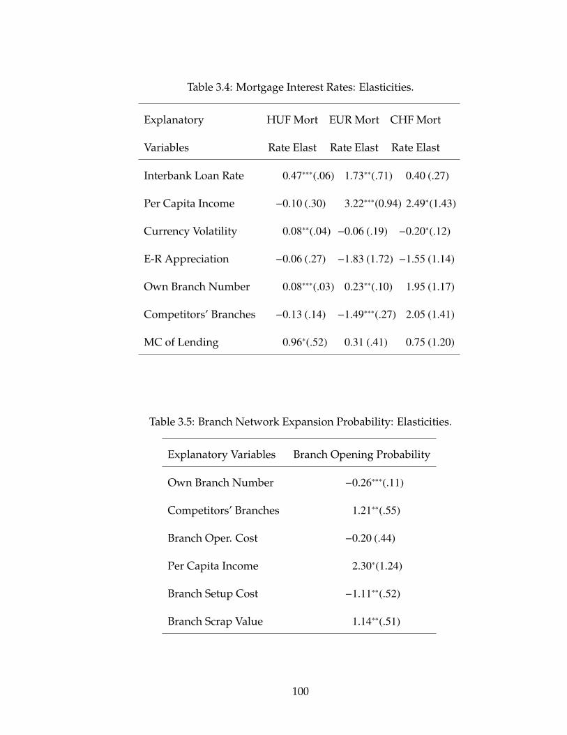
Table 3.4: Mortgage Interest Rates: Elasticities.

Explanatory HUF Mort EUR Mort CHF Mort

Variables Rate Elast Rate Elast Rate Elast

Interbank Loan Rate 0.47∗∗∗(.06) 1.73∗∗(.71) 0.40 (.27)

Per Capita Income −0.10 (.30) 3.22∗∗∗(0.94) 2.49∗(1.43)

Currency Volatility 0.08∗∗(.04) −0.06 (.19) −0.20∗(.12)

E-R Appreciation −0.06 (.27) −1.83 (1.72) −1.55 (1.14)

Own Branch Number 0.08∗∗∗(.03) 0.23∗∗(.10) 1.95 (1.17)

Competitors’ Branches −0.13 (.14) −1.49∗∗∗(.27) 2.05 (1.41)

MC of Lending 0.96∗(.52) 0.31 (.41) 0.75 (1.20)

Table 3.5: Branch Network Expansion Probability: Elasticities.

Explanatory Variables Branch Opening Probability

Own Branch Number −0.26∗∗∗(.11)

Competitors’ Branches 1.21∗∗(.55)

Branch Oper. Cost −0.20 (.44)

Per Capita Income 2.30∗(1.24)

Branch Setup Cost −1.11∗∗(.52)

Branch Scrap Value 1.14∗∗(.51)

100

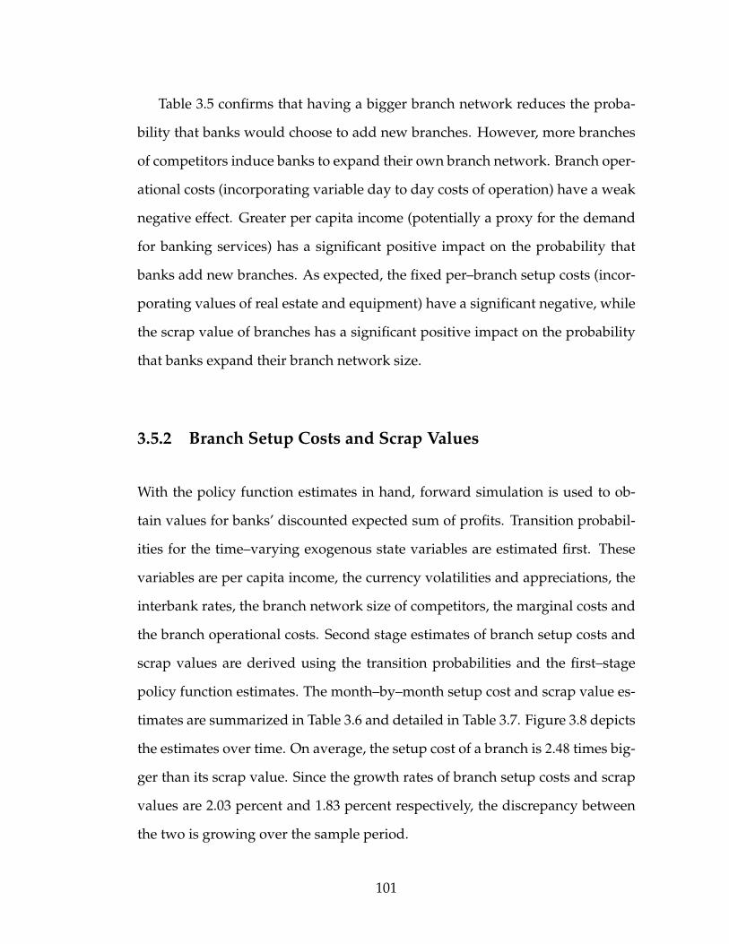
Table 3.5 confirms that having a bigger branch network reduces the proba-

bility that banks would choose to add new branches. However, more branches

of competitors induce banks to expand their own branch network. Branch oper-

ational costs (incorporating variable day to day costs of operation) have a weak

negative effect. Greater per capita income (potentially a proxy for the demand

for banking services) has a significant positive impact on the probability that

banks add new branches. As expected, the fixed per–branch setup costs (incor-

porating values of real estate and equipment) have a significant negative, while

the scrap value of branches has a significant positive impact on the probability

that banks expand their branch network size.

3.5.2 Branch Setup Costs and Scrap Values

With the policy function estimates in hand, forward simulation is used to ob-

tain values for banks’ discounted expected sum of profits. Transition probabil-

ities for the time–varying exogenous state variables are estimated first. These

variables are per capita income, the currency volatilities and appreciations, the

interbank rates, the branch network size of competitors, the marginal costs and

the branch operational costs. Second stage estimates of branch setup costs and

scrap values are derived using the transition probabilities and the first–stage

policy function estimates. The month–by–month setup cost and scrap value es-

timates are summarized in Table 3.6 and detailed in Table 3.7. Figure 3.8 depicts

the estimates over time. On average, the setup cost of a branch is 2.48 times big-

ger than its scrap value. Since the growth rates of branch setup costs and scrap

values are 2.03 percent and 1.83 percent respectively, the discrepancy between

the two is growing over the sample period.

101

Feb2004 Sep2004 Mar2005 Oct2005 May2006 Nov2006 Jun2007 Dec20070

50

100

150

200

250

300

Time Period

Est

imat

es (

Mill

ions

of H

UF

)

Est. Branch Setup CostEst. Branch Scrap Value

Figure 3.8: Estimated Branch Setup Costs and Scrap Values Over Time.

Table 3.6: Summary Statistics (Millions of HUF).

Parameter Min 25p 50p 75p Max Mean Std Dev

Setup Cost 80.00 107.86 147.23 182.03 218.43 148.81 41.92

Scrap Value 60.00 83.70 110.43 129.63 149.54 109.48 25.37

Table 3.7: Branch Setup Cost and Scrap Value Estimates (Millions of HUF).

Time Period Branch Setup Cost Branch Scrap Value

Jan 04 80.00∗∗∗(.18) 60.00∗∗∗(1.53)

Feb 04 100.51∗∗∗(.27) 80.01∗∗(37.97)

Mar 04 101.68∗∗∗(.44) 80.86∗∗∗(18.63)

102

Table 3.7: (Continued)

Time Period Branch Setup Cost Branch Scrap Value

Apr 04 103.07∗∗∗(.54) 80.51 (212.51)

May 04 104.60∗∗∗(.48) 81.03 (155.75)

June 04 106.00∗∗∗(.59) 81.78 (123.38)

July 04 107.39∗∗∗(.70) 82.64 (122.52)

Aug 04 107.86∗∗∗(1.18) 83.16∗∗∗(23.76)

Sept 04 107.86∗∗∗(1.43) 83.13∗∗∗(30.25)

Oct 04 107.86∗∗∗(1.18) 84.58∗∗∗(22.02)

Nov 04 107.86∗∗∗(1.17) 83.70∗∗∗(21.34)

Dec 04 107.86∗∗∗(1.28) 82.83∗∗∗(19.37)

Jan 05 107.40∗∗∗(3.08) 84.39∗∗∗(31.97)

Feb 05 106.48∗∗∗(6.12) 83.90 (95.76)

Mar 05 105.10∗∗∗(4.63) 83.14∗∗∗(13.28)

Apr 05 109.29∗∗∗(3.19) 86.15∗∗∗(19.62)

May 05 116.75∗∗∗(1.19) 88.52∗∗∗(15.38)

June 05 126.38∗∗∗(1.38) 97.43 (81.12)

July 05 137.09∗∗∗(3.64) 102.94∗∗∗(13.72)

Aug 05 147.23∗∗∗(1.96) 110.43∗∗∗(16.91)

Sept 05 155.13∗∗∗(4.56) 115.86 (156.58)

Oct 05 158.86∗∗∗(5.79) 118.06 (152.53)

103

Table 3.7: (Continued)

Time Period Branch Setup Cost Branch Scrap Value

Nov 05 158.86∗∗∗(6.01) 118.06 (100.93)

Dec 05 158.86∗∗∗(6.78) 118.06 (86.94)

Jan 06 158.86∗∗∗(8.70) 118.06 (151.06)

Feb 06 158.86∗∗∗(10.28) 118.06 (332.71)

Mar 06 157.67∗∗∗(8.87) 117.12 (195.01)

Apr 06 151.56∗∗∗(8.94) 113.03∗(67.60)

May 06 142.90∗∗∗(14.68) 107.31 (138.27)

June 06 133.52∗∗∗(8.73) 101.16 (139.56)

July 06 137.70∗∗∗(8.17) 102.34 (111.63)

Aug 06 123.25∗∗∗(13.60) 108.70 (100.37)

Sept 06 158.82∗∗∗(12.53) 115.12 (88.44)

Oct 06 167.93∗∗∗(13.27) 120.52 (92.76)

Nov 06 175.26∗∗∗(16.26) 125.27 (81.22)

Dec 06 182.03∗∗∗(4.91) 129.63 (70.28)

Jan 07 188.98∗∗∗(9.77) 133.95 (135.63)

Feb 07 196.59∗∗∗(11.76) 138.54 (85.84)

Mar 07 204.79∗∗∗(25.50) 143.35∗∗∗(14.86)

Apr 07 214.48∗∗∗(11.14) 148.21∗∗∗(18.59)

May 07 218.42∗∗∗(13.17) 149.54∗∗∗(23.56)

104

Table 3.7: (Continued)

Time Period Branch Setup Cost Branch Scrap Value

June 07 218.42∗∗∗(8.08) 149.54∗∗∗(25.72)

July 07 218.42∗∗∗(11.26) 149.54∗∗∗(18.77)

Aug 07 218.42∗∗∗(9.67) 149.54∗∗∗(27.01)

Sept 07 218.42∗∗∗(9.94) 149.54∗∗∗(54.88)

Oct 07 214.94∗∗∗(8.15) 146.68∗∗(69.74)

Nov 07 203.65∗∗∗(9.46) 139.44∗(76.19)

Table 3.8 shows the relationship between measures of the cost of construc-

tion, and estimates of the branch setup costs and scrap values. Setup cost and

scrap value estimates are strongly positively correlated, and both move closely

with relevant producer price indices.

Table 3.8: Correlations.

Measures Setup Cost Scrap Value

Scrap Value 0.99∗∗∗

Manufacturing PPI 0.89∗∗∗ 0.90∗∗∗

Industrial PPI 0.92∗∗∗ 0.93∗∗∗

Investment PPI 0.88∗∗∗ 0.90∗∗∗

105

3.6 Simulation Exercises

This section explores the impact of increasing various model parameters on

banks’ optimal behavior. In particular, arc elasticities of bank interest rate and

branch network size choices with respect to setup costs, consumer income, and

competitors’ branch network size are reported.

3.6.1 Increasing Branch Setup Costs

This subsection examines the effect of a one–time increase in the initial value of

branch setup cost on the behavior of the average bank throughout the course

of the sample period. Figure 3.9 displays the negative relationship between

setup cost increases and the arc elasticity of the probability of branch network

expansion. The arc elasticity is small, and decreasing in magnitude – implying

that expansion probabilities are concave in setup costs.

0 10 20 30 40 50 60 70 80 90 100−0.018

−0.017

−0.016

−0.015

−0.014

−0.013

−0.012

Percent Increase In Initial Setup Cost

Ela

stic

ity

Elast. of Avg. Prob. ofOpening Branches

Figure 3.9: Elasticity of Branch Opening Probability w.r.t. Setup Cost.

106

3.6.2 Increasing Consumer Income

This exercise explores the effects of gradual percent increases in per capita con-

sumer income on indicators of bank profitability and bank behavior. Increases

in income impact the choices of all interest rates, as well the the size of the

branch network. Figure 3.10 explores the impact of increases in per capita in-

come on the average bank’s Net Interest Income (NII), a common measure of

profitability. It shows that at low levels of initial income, a 1 percent increase in

income raises NII by 2.5 percent over the length of the sample period (strongly

elastic). However, this arc elasticity decreases with income, to a steady level of

0.25 in the inelastic range – implying that NII is increasing concave in consumer

income.

0 10 20 30 40 50 60 70 80 90 1000

0.5

1

1.5

2

2.5

3

Percent Increase in Per Capita Income

Ela

stic

ity

Elast. of Bank Net InterestIncome w.r.t Consumer Inc.

Figure 3.10: Elasticity of Net Interest Income w.r.t. Per Capita ConsumerIncome.

Figure 3.11 explores the effect of increases in income on the elasticity of the

107

average bank’s own branch network size. The depicted positive relationship is

in line with the results presented in Table 3.5. The per capita income arc elas-

ticity of branch network size increases from 0.31 to 0.35 as income increases

(consistently in the inelastic range) — implying that branch network size is in-

creasing convex in consumer income.

0 10 20 30 40 50 60 70 80 90 1000.305

0.31

0.315

0.32

0.325

0.33

0.335

0.34

0.345

Percent Increase in Per Capita Income

Ela

stic

ity

Elast. of Avg. Branch NetworkSize w.r.t. Per Capita Income

Figure 3.11: Elasticity of Branch Network Size w.r.t. Per Capita ConsumerIncome.

0 10 20 30 40 50 60 70 80 90 100−0.4

−0.2

0

Percent Increase in Per Capita Income

Ela

stic

ity

0 10 20 30 40 50 60 70 80 90 1000

5

10

Ela

stic

ity

Lending Rate Elast Deposit Rate Elast Mortgage Rate Elast

Figure 3.12: Elasticities of Interest Rates w.r.t. Per Capita Consumer In-come.

108

Figure 3.12 shows the impact of income increases on banks’ choices of inter-

est rates. Both the average retail lending and deposit rates respond negatively to

rises in income, depicting a negative concave relationship. Mortgage rates, on

the other hand, are strongly elastic and increasing convex in consumer income.

These results are in line with the estimates presented in Section 3.5.

3.6.3 Increasing Competitors’ Branch Network Size

This simulation exercise explores the impact of increases in competitors’ branch

network size on the average bank’s optimal behavior. Figure 3.13 shows how

the average bank’s Net Interest Income (NII) responds to increases in the branch

network size of competitors. At the observed numbers of competitors’ branches,

a 1 percent increase in their network size causes average bank NII to fall by

over 8 percent. However, this negative impact dampens quickly as competitors’

network size rises. In fact, at numbers twice as big as the observed values,

the response of average bank NII to rises in competitors’ branch network size

becomes positive.

Figure 3.14 shows the impact of competitors’ branch network size on the

own network size of the average bank. This effect is weakly positive, and

greater at higher levels of competitors’ network size (in the 0.23 to 0.25 range) —

implying an increasing convex relationship in line with Table 3.5. It appears that

branch network competition becomes more intense when the overall branch

network is greater.

Figure 3.15 depicts the impact of rises in competitors’ branch network size

109

0 10 20 30 40 50 60 70 80 90 100

−8

−6

−4

−2

0

2

Percent Increase in Competitors’ Branch Network Size

Ela

stic

ity

Elast. of Net Interes Incomew.r.t. Competitors’ BranchNetwork Size

Figure 3.13: Elasticity of Net Interest Income w.r.t. Competitors’ BranchNetwork Size.

0 10 20 30 40 50 60 70 80 90 100

0.23

0.235

0.24

0.245

Percent Increase in Competitors’ Branch Network Size

Ela

stic

ity

Elast. of Bank’s Own BranchNetwork w.r.t. Competitors’ Branch Network Size

Figure 3.14: Elasticity of Branch Network Size w.r.t. Competitors’ BranchNetwork Size.

on the average bank’s choices of interest rates. As expected, the average bank

offers higher deposit rates and demands lower loan rates as the number of com-

petitors’ branches increases. Mortgage rates, however, respond positively on

average. This is due to the strong positive elasticity of CHF mortgages which

outweighs the negative response of HUF and EUR mortgages, as described in

110

Section 3.5 above.

0 10 20 30 40 50 60 70 80 90 100−0.2

0

0.2

Percent Increase in Competitors’ Branch Network Size

Ela

stic

ities

0 10 20 30 40 50 60 70 80 90 1000

0.5

1

Ela

stic

ities

Elast. of Avg. Retail Loan RatesElast. of Avg. Deposit RatesElast. of Avg. Mortgage Rates

Figure 3.15: Elasticity of Interest Rates w.r.t. Competitors’ Branch Net-work Size.

Comparing the effects of increases in per capita consumer income and com-

petitors’ branch network size, it is interesting to note that the signs of the im-

pacts are very similar (with the notable exception of the response of retail lend-

ing rates). However, the magnitudes are rather different. The effects of per

capita consumer income increases are consistently greater than the impacts of

increases in competitors’ branch network size.

3.7 Summary

The purpose of this chapter is to provide a thorough examination of the com-

petitive behavior of Hungarian commercial banks in a dynamic framework. The

study presented in this chapter contributes to the previous literature by incorpo-

rating branch network competition (in addition to interest rate competition) of

imperfectly competitive commercial banks in a dynamic setting. Furthermore,a

111

model–based approach is used to estimate structural parameters (branch setup

costs and scrap values) that so far have been only approximated by ad hoc em-

pirical measures.

The chapter develops a model of branch network and interest rate competi-

tion, where banks simultaneously make retail lending, mortgage, deposit inter-

est rate, as well as branch network size decisions. Banks take into account the

impact of their choices on their future profits. Banks’ optimal interest rate and

branch network size choices are characterized in the Salop competition frame-

work. Comparative statics predictions about the impact of the model’s state

variables (such as marginal costs, branch operational costs, interbank rates) on

banks’ optimal choices are derived. A version of the Bajari, Benkard, and Levin

(2007) two–stage estimation method is developed to estimate the policy equa-

tions, and to obtain estimates of the branch setup costs and scrap values.

Results corresponding to the first stage of the estimation (the static policy

function estimates) show that own and competitors’ branch network sizes have

a strong impact on banks’ interest rate choices. This finding confirms the con-

clusions of the previous literature (Dick, 2007; Spieker, 2004) that consumers

care much about the proximity and availability of bank branches (which banks

charge a premium for). When competitors have more branches, the average

bank compensates by lowering its lending rates and paying higher rates on

deposits. Furthermore, banks’ propensity to build new branches decreases in

the size of their existing network. Competition in bank branch network size is

confirmed by the result that greater branch network size of competitors induce

banks to expand their own network as well. Furthermore, banks add fewer new

branches if their operation is more expensive, and if branches cost more to build.

112

Banks are more likely to add new branches if the scrap values are high.

The second stage of the dynamic estimation obtains estimates of the fixed

setup costs (and scrap values) of bank branch network expansion (and contrac-

tion). The per–bank setup cost (with an average of approximately 150 million

HUF, or about 0.75 million USD) is 2.48 times greater than the mean scrap value

(with an average of 110 million HUF, or approximately 0.55 million USD). As

branch setup costs grow faster than scrap values, the discrepancy between the

two is growing over the sample period.

Simulation exercises are conducted to examine the impacts of rises in branch

setup costs, per capita consumer income and competitors’ branch network size

on the optimal behavior of the average bank. Branch setup costs only have a

very small negative impact on bank profitability (as measured by Net Interest

Income), and negligible effect on interest rates. The choice of branch network

size has a negative response, as expected. Rising per capita consumer income

and competitors’ branch network size have strong effects on bank behavior —

confirming the important roles of consumer traits (the demand side) and com-

petitive behavior (the supply side). This chapter provides a careful study of the

credit supply side — a contribution to a literature that focuses heavily on the

demand (consumer) side of banking in Hungary. The results presented in this

paper can therefore have important policy implications from the perspective of

bank regulators.

113

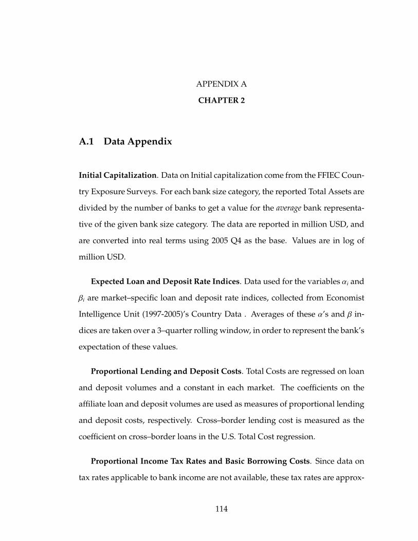
APPENDIX A

CHAPTER 2

A.1 Data Appendix

Initial Capitalization. Data on Initial capitalization come from the FFIEC Coun-

try Exposure Surveys. For each bank size category, the reported Total Assets are

divided by the number of banks to get a value for the average bank representa-

tive of the given bank size category. The data are reported in million USD, and

are converted into real terms using 2005 Q4 as the base. Values are in log of

million USD.

Expected Loan and Deposit Rate Indices. Data used for the variables αi and

βi are market–specific loan and deposit rate indices, collected from Economist

Intelligence Unit (1997-2005)’s Country Data . Averages of these α’s and β in-

dices are taken over a 3–quarter rolling window, in order to represent the bank’s

expectation of these values.

Proportional Lending and Deposit Costs. Total Costs are regressed on loan

and deposit volumes and a constant in each market. The coefficients on the

affiliate loan and deposit volumes are used as measures of proportional lending

and deposit costs, respectively. Cross–border lending cost is measured as the

coefficient on cross–border loans in the U.S. Total Cost regression.

Proportional Income Tax Rates and Basic Borrowing Costs. Since data on

tax rates applicable to bank income are not available, these tax rates are approx-

114

Table A.1: Loan & Deposit Averages by Country Over Time (log millionsof 2005 Q4 USD).

Code Aff. Loan CB Loan Dep. Code Aff. Loan CB Loan Dep.

AR 4.79 4.80 5.20 JA 4.87 5.45 4.58

AU 4.92 4.90 5.00 LU 2.50 3.86 4.38

AT 1.57 4.63 1.68 MY 2.87 2.79 2.72

BE 2.01 5.18 3.00 MX 4.77 5.88 4.47

BR 6.78 5.72 6.89 NL 2.16 6.08 3.02

BG 2.52 0.85 2.96 NZ 3.85 2.56 3.12

CA 6.30 5.80 6.05 NO 1.99 3.86 1.12

CL 5.86 4.19 5.85 PH 5.43 3.88 5.41

CN 4.21 3.29 3.33 PL 6.38 1.71 6.28

CO 4.51 3.73 4.23 PT 4.55 3.31 4.68

CZ 5.22 1.22 5.59 RO 3.85 0.51 3.93

DK 1.13 4.73 0.81 RU 4.39 2.81 4.26

FI −0.34 3.11 −0.05 SG 3.51 4.34 4.64

FR 2.54 5.99 2.41 SK 4.44 1.14 4.38

DE 4.02 6.50 4.25 ZA 5.64 3.09 5.96

GR 6.14 3.21 6.46 KR 4.22 5.11 2.95

HU 5.00 1.11 5.18 ES 4.30 4.47 3.62

IS −1.29 0.98 −1.15 SE 2.14 4.65 1.52

IN 6.44 3.59 6.83 CH. 2.66 5.08 2.28

ID 5.35 3.06 5.69 TH 2.02 2.74 1.86

IE 3.15 4.60 3.42 TR 5.17 4.20 5.04

IL 4.38 3.69 3.91 UK 7.13 7.21 7.46

IT 4.02 5.05 2.98 US 11.57 − 11.57

115

Table A.2: Loan & Deposit Averages by Time Period Across Countries (logmillions of 2005 Q4 USD).

Time Aff Loans CB Loans Deps Time Aff Loans CB Loans Deps

97/12 4.38 3.59 4.42 02/03 4.15 3.98 4.21

98/03 4.29 3.65 4.43 02/06 4.13 3.96 4.42

98/06 4.18 3.74 4.13 02/09 4.16 3.95 4.31

98/09 4.27 3.69 4.40 02/12 4.35 3.91 4.31

98/12 4.31 3.67 4.44 03/12 4.45 3.92 4.36

99/12 4.36 3.66 4.22 03/06 4.43 3.96 4.37

99/06 4.24 3.71 4.45 03/09 4.35 4.00 4.37

99/12 4.39 3.73 4.60 03/12 4.38 4.09 4.41

99/12 4.47 3.67 4.51 04/03 4.29 4.11 4.26

00/03 3.83 3.66 4.16 04/06 4.46 4.15 4.33

00/06 4.52 3.08 4.09 04/09 4.77 4.24 4.06

00/09 4.12 3.80 3.81 04/12 4.66 4.17 4.46

00/12 4.31 3.69 3.94 05/12 4.54 4.26 4.48

01/03 4.31 3.80 3.99 05/06 4.25 4.20 4.41

01/06 4.27 3.95 4.43 05/09 4.51 4.31 4.54

01/09 4.10 3.92 4.22 05/12 4.45 4.30 4.86

01/12 3.19 3.98 3.11

116

Table A.3: Summary of Explanatory Variables.

Variable Name Note Empirical Measure

Cross-Border Loan in i licb j Bank’s CB claims in i, mill 2005 USD

Affiliate Loan in i lia j Bank’s claims in i, mill 2005 USD

Foreign Aff Dep’ in i dij Bank’s FA liabs in i, mill 2005 USD

Bank Scope S j Lagged Sharpe Ratio

Initial Bank Capital K j Bank’s Total Assets, mill 2005 USD

Expected Aff αia Mean of predicted aff loan

Loan market return in i mkt return in i over 3-qtr window

Expected Deposit βia Mean of predicted deposit

market return in i mkt return in i over 3-qtr window

Expected CB Loan αicb Mean of predicted CB loan

market return in i mkt return in i over 3-qtr window

Lending Cost cil j Stock mkt Return in i - ROA

Deposit-taking cost cid Deposit rate - money mkt rate

Income Tax Rate ti Corporate Tax Rate in i

Req. Reserve Ratio in i δi Required Reserve Ratio in i

Bank’s Risk Aversion λ j Estimated from Model

Capital Adequacy ki Minimum Cap. Ratio in i

Basic Cost of Other ri∆

Basic ’riskless’ interest rate set by

Borrowing in i the monetary authority in i

Loan Deman Elast. ε im Estimated Coefficient

Deposit S. Elast in Deposit ηi Estimated Coefficient

Regulator’s Risk Avers. in i θi Estimated from Model

Entry Cost & Scrap Value in i Γi Estimated from Model

117

imated with corporate income tax rates taken from the Organisation for Eco-

nomic Co-operation and Development (1997-2005)’s database. The basic cost

of non–deposit borrowing is measured using the country–specific equivalent of

the federal funds rate, set by the monetary authority in market i (the equivalent

of the federal funds rate). Data on these interest rates are collected from the

International Monetary Fund (1997-2005)’s International Financial Statistics.

Required Reserve Ratio and Minimum Capital Ratio. Data on market–

specific required reserve ratios and minimum capital ratios are collected from

the World Bank (1997-2005)’s Bank Regulation and Supervision database. Where

not available, the ratios are directly taken from national central banks’ websites.

Data on Loan Demand and Deposit Supply Elasticities. Taking logs of the

Dixit-Stiglitz form of the loan demand equation yields: log lim = logαi

m − εi · ri

lm

where rilm is the lending rate in market m. The coefficient ε i

m from this regres-

sion is used as loan demand elasticity. Similarly, the deposit supply equation is

log di = log βi + ηi · rid

, from which the deposit supply elasticity in country i is

measured as the coefficient ηi.

Bank Scope. Initial bank scope is measured as the lagged Sharpe ratio.

Loan & Deposit Volumes. Tables A.1 and A.2 present averages of the loans

& deposits by country and by time period, respectively. Table A.3 summarizes

notation and empirical measures used for the explanatory variables in this chap-

ter.

Summary Statistics. Table A.4 presents summary statistics.

118

Table A.4: Summary Statistics of Variables.

Name Min 25p 50p 75p Max Std Dev

Log of CB Loans −4.25 1.85 4.25 6.13 9.06 2.85

Log of Affil Loans −4.44 1.58 4.99 6.70 13.58 3.52

Log of Affil Dep’s −4.44 1.37 5.11 6.71 13.61 3.59

Log of Bank Capital 9.60 9.99 10.39 12.99 13.84 1.47

Exp. Loan market 1.38 5.60 8.30 13.30 97.7 15.21

return in i

Exp. Deposit 0.06 2.25 3.67 7.75 87.36 10.64

return in i

Exp. CB Loan 0.02 2.7 4.59 7.67 174.72 12.80

return in i

Proportional Cost 0.09 0.38 0.72 1.79 30.21 2.76

Income Tax Rate 10 28 33 35.70 57.5 7.38

Req Reserve Ratio 0 2 4 10 34 7.51

Min Capital Ratio 8 8 8 8 16 1.45

Nondep Borrow Cost 0 4.24 5.40 8.26 105.72 12.87

Affil Loan Elast in i 0 .05 0.27 0.55 8.68 1.27

Dep Supply Elast 0 0.06 0.30 1.15 2.96 0.78

CB Loan Elast 0 0.05 0.09 0.19 1.99 0.32

Lag Sharpe Ratio 2.78 3.23 3.32 3.70 3.78 0.27

Sharpe Ratio

119

APPENDIX B

CHAPTER 3

B.1 Model Appendix

Using the optimality condition in (3.15), the Implicit Function Theorem implies

∂rhl j

∂n j= −

∂E

(Lh

j

)∂n j

+(rh

l j − r − chl j

) ∂2E(Lh

j

)∂rh

l j∂n j

2∂E

(Lh

j

)∂rh

l j+

(rh

l j − r − chl j

) ∂2E(Lh

j

)∂rh2

l j

> 0

∂rhl j

∂r=∂rh

l j

∂chl j

= −

−∂E

(Lh

j

)∂rh

l j

2∂E

(Lh

j

)∂rh

l j+

(rh

l j − r − chl j

) ∂2E(Lh

j

)∂rh2

l j

> 0

∂rhl j

∂n− j= −

∂E

(Lh

j

)∂n− j

+(rh

l j − r − chl j

) ∂2E(Lh

j

)∂rh

l j∂n− j

2∂E

(Lh

j

)∂rh

l j+

(rh

l j − r − chl j

) ∂2E(Lh

j

)∂rh2

l j

< 0

∂rhl j

∂I= −

∂E

(Lh

j

)∂I +

(rh

l j − r − chl j

) ∂2E(Lh

j

)∂rh

l j∂I

2∂E

(Lh

j

)∂rh

l j+

(rh

l j − r − chl j

) ∂2E(Lh

j

)∂rh2

l j

> 0

(B.1)

In all of the derivatives in Equation (B.1), the denominators are negative due

to the second–order condition for a maximum holding. Equation (3.12) implies

that the numerator in the top row of (B.1) is positive. Therefore, bank j’s own

rate increases in the number of branches it operates. By the law of demand, the

numerator in the second row of (B.1) is positive — therefore, the optimal retail

lending rate increases in both the interbank lending rate and the marginal cost

of retail lending. Equation (3.12) implies that the numerator in the third row of

(B.1) is negative — therefore, larger branch network size by other banks causes

bank j to lower its optimal choice of the retail lending rate. In the bottom row

120

of Equation (B.1), the sign of the numerator is positive — therefore, higher per

capita income leads to higher lending rates.

∂rhd j

∂n j= −

−∂E

(Dh

j

)∂n j

+(r (1 − φ) − rh

d j − chd j

) ∂2E(Dh

j

)∂rh

d j∂n j

−2∂E

(Dh

j

)∂rh

d j+

(r (1 − φ) − rh

d j − chd j

) ∂2E(Dh

j

)∂rh2

d j

< 0

∂rhd j

∂r= −

(1 − φ)

∂E(Dh

j

)∂rh

d j

−2∂E

(Dh

j

)∂rh

d j+

(r (1 − φ) − rh

d j − chd j

) ∂2E(Dh

j

)∂rh2

d j

> 0

∂rhd j

∂chl j

= −

−∂E

(Dh

j

)∂rh

d j

−2∂E

(Dh

j

)∂rh

d j+

(r (1 − φ) − rh

d j − chd j

) ∂2E(Dh

j

)∂rh2

d j

< 0

∂rhd j

∂n− j= −

−∂E

(Dh

j

)∂n− j

+(r (1 − φ) − rh

d j − chd j

) ∂2E(Dh

j

)∂rh

d j∂n− j

−2∂E

(Dh

j

)∂rh

d j+

(r (1 − φ) − rh

d j − chd j

) ∂2E(Dh

j

)∂rh2

d j

> 0

∂rhd j

∂I= −

−∂E

(Dh

j

)∂I +

(r (1 − φ) − rh

d j − chd j

) ∂2E(Dh

j

)∂rh

d j∂I

−2∂E

(Dh

j

)∂rh

d j+

(r (1 − φ) − rh

d j − chd j

) ∂2E(Dh

j

)∂rh2

d j

< 0

(B.2)

In all the derivatives in Equation (B.2), the denominators are negative due

to the second-order condition for a maximum holding. Equation (3.13) implies

that the numerator in the top row of Equation (B.2) is negative. Therefore, bank

j’s own deposit rate decreases in the number of branches it operates. By the law

of supply, the numerator in the second row is positive — therefore, the optimal

deposit rate increases in the interbank rate. By the same reasoning, the numer-

ator in the third row of Equation (B.2) is negative — implying that the opti-

mal deposit rate decreases in the marginal cost of retail lending. Equation(3.13)

implies that the numerator in the fourth row of Equation (B.2) is positive —

therefore, larger branch network size of competitors causes bank j to increase

121

its optimal choice of the retail deposit rate. Finally, the numerator in the bottom

row of Equation (B.2) is negative, implying that an increase in per capita income

causes bank j to lower its optimal retail deposit rate.

B.2 Data Appendix

This section gives a detailed description of the data used in the estimation of the

model.

Interest Rates. Bank–level data on interest rates come from the PSzAF regu-

latory database. Interest rates are measured by the Effective Annual Percentage

Rate (APR) for loans, and Effective Annual Percentage Yield (APY) for deposits.

These measures are calculated on an annual basis, and also account for fees.

Bank Branch Network Size. Bank–level data come from the PSzAF regula-

tory database. Data on the total number of bank branches in Hungary comes

from the online database of Magyar Nemzeti Bank (2004-2007). Data on com-

petitors’ branch network size are calculated using both these sources.

Interbank Rates and Reserve Requirements. Data come from the MNB.

Currency Volatilities and Appreciation. Volatilities of the Hungarian Forint,

the Swiss Franc and the Euro are measured as the standard deviation of the ex-

change rate between these currencies and the U.S. Dollar over the six months

preceding the period. Exchange rate data come from the MNB.

Per Capita Income. Data come from the Hungarian KSH’s online database.

Bank Discount Factor and Proportional Costs. Bank–specific discount fac-

122

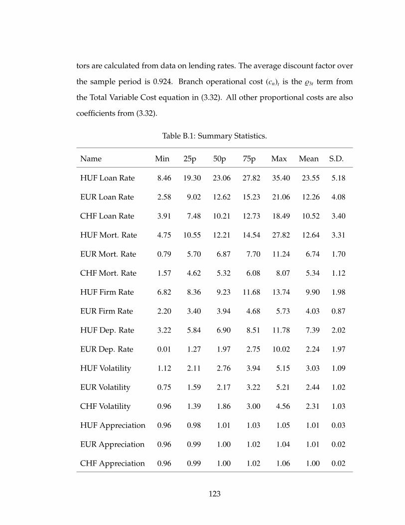
tors are calculated from data on lending rates. The average discount factor over

the sample period is 0.924. Branch operational cost (cn)t is the %3t term from

the Total Variable Cost equation in (3.32). All other proportional costs are also

coefficients from (3.32).

Table B.1: Summary Statistics.

Name Min 25p 50p 75p Max Mean S.D.

HUF Loan Rate 8.46 19.30 23.06 27.82 35.40 23.55 5.18

EUR Loan Rate 2.58 9.02 12.62 15.23 21.06 12.26 4.08

CHF Loan Rate 3.91 7.48 10.21 12.73 18.49 10.52 3.40

HUF Mort. Rate 4.75 10.55 12.21 14.54 27.82 12.64 3.31

EUR Mort. Rate 0.79 5.70 6.87 7.70 11.24 6.74 1.70

CHF Mort. Rate 1.57 4.62 5.32 6.08 8.07 5.34 1.12

HUF Firm Rate 6.82 8.36 9.23 11.68 13.74 9.90 1.98

EUR Firm Rate 2.20 3.40 3.94 4.68 5.73 4.03 0.87

HUF Dep. Rate 3.22 5.84 6.90 8.51 11.78 7.39 2.02

EUR Dep. Rate 0.01 1.27 1.97 2.75 10.02 2.24 1.97

HUF Volatility 1.12 2.11 2.76 3.94 5.15 3.03 1.09

EUR Volatility 0.75 1.59 2.17 3.22 5.21 2.44 1.02

CHF Volatility 0.96 1.39 1.86 3.00 4.56 2.31 1.03

HUF Appreciation 0.96 0.98 1.01 1.03 1.05 1.01 0.03

EUR Appreciation 0.96 0.99 1.00 1.02 1.04 1.01 0.02

CHF Appreciation 0.96 0.99 1.00 1.02 1.06 1.00 0.02

123

Table B.1: (Continued)

Name Min 25p 50p 75p Max Mean S.D.

MC of Retail Loans 19.61 21.03 22.41 23.20 24.00 21.99 1.25

MC of Mortgages 8.17 8.76 9.34 9.67 10 9.16 0.52

MC of Deposits 1.63 1.75 1.86 1.93 2.00 1.83 0.10

Own Branch (100’s) 0.32 0.68 1.53 1.82 4.33 1.72 1.30

Competitors’ 7.06 10.57 11.26 12.96 14.66 11.42 18.84

Branches (100’s)

Per capita Income 0.06 0.06 0.06 0.06 0.07 0.06 0.01

Branch Oper. Cost 12.76 17.50 19.54 21.24 32.37 19.51 3.53

Branch Expansion −6 0 1 1 6 0.67 1.74

Table B.2: Summary of Interest Rates by Time Period.

Time HUF EUR CHF HUF EUR HUF EUR CHF HUF EUR

Loan Loan Loan Firm Firm Mor Mor Mor Dep Dep

04/01 22.43 − − 11.68 − 13.90 − − 9.03 −

04/02 24.64 − − 12.91 − 15.76 − − 10.01 −

04/03 25.39 − − 13.68 − 19.81 − − 11.07 −

04/04 26.85 − − 13.74 − 17.45 − − 10.61 −

04/05 26.12 − − 12.84 − 15.83 − − 10.09 −

04/06 26.45 − − 13.45 − 16.82 − − 10.50 −

124

Table B.2: (Continued)

Time HUF EUR CHF HUF EUR HUF EUR CHF HUF EUR

Loan Loan Loan Firm Firm Mor Mor Mor Dep Dep

04/07 26.73 − − 13.48 − 16.39 − − 10.56 −

04/08 27.32 − − 13.63 − 16.62 − − 10.86 −

04/09 27.61 − − 13.15 − 14.24 − − 9.90 −

04/10 26.86 − − 12.45 − 14.23 − − 9.35 −

04/11 26.89 − − 12.44 − 14.53 − − 9.25 −

04/12 29.21 − − 12.07 − 14.05 − − 9.21 −

05/01 26.15 10.54 9.37 10.86 2.85 13.40 6.58 5.66 8.12 0.61

05/02 24.74 11.23 10.19 10.67 3.15 13.10 6.35 5.39 7.67 0.93

05/03 24.16 13.91 10.21 9.77 2.87 12.67 6.53 5.48 7.22 2.51

05/04 22.61 10.85 10.23 9.23 2.80 12.05 8.46 5.16 6.37 0.67

05/05 22.68 10.08 11.44 9.13 2.98 13.18 6.53 4.85 6.53 0.90

05/06 23.00 12.18 10.62 9.2 3.31 13.26 6.64 5.51 6.43 1.14

05/07 20.39 10.93 11.11 9.2 3.57 15.38 6.97 5.82 6.13 1.56

05/08 20.88 13.12 10.62 9.26 4.00 14.50 7.53 6.18 6.44 1.88

05/09 23.93 11.46 10.30 8.27 3.40 12.64 7.04 5.65 5.47 2.29

05/10 21.36 11.55 10.13 8.32 3.76 12.09 7.19 6.28 5.18 1.46

05/11 22.73 11.91 9.7 8.09 3.51 10.81 5.95 5.77 6.22 1.35

05/12 22.63 10.67 10.14 8.23 3.90 10.83 6.57 5.88 5.70 1.72

06/01 21.92 11.42 10.20 8.08 3.82 10.96 7.27 5.77 5.56 1.68

06/02 23.10 11.53 10.82 7.95 3.74 10.86 7.42 5.66 5.42 1.53

06/03 22.58 13.21 10.97 7.55 3.50 11.05 7.06 5.31 5.08 1.20

125

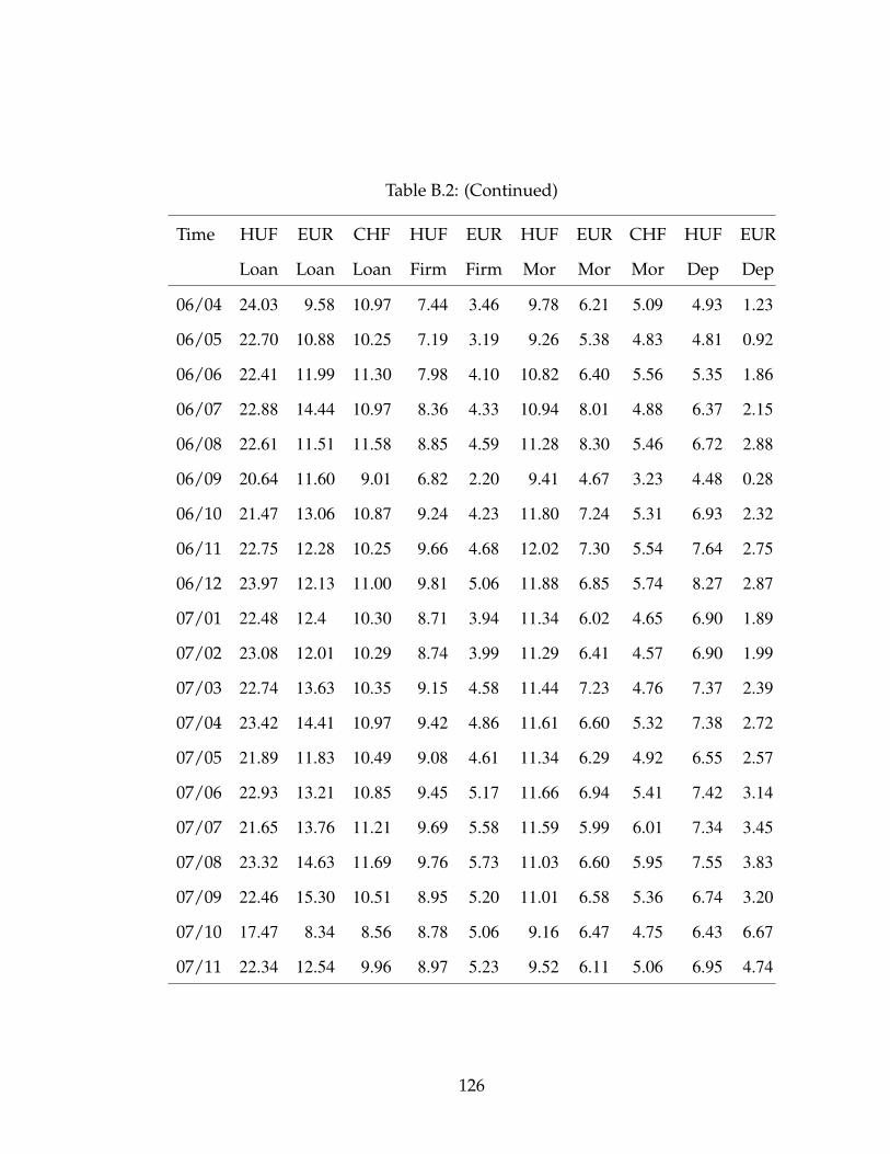
Table B.2: (Continued)

Time HUF EUR CHF HUF EUR HUF EUR CHF HUF EUR

Loan Loan Loan Firm Firm Mor Mor Mor Dep Dep

06/04 24.03 9.58 10.97 7.44 3.46 9.78 6.21 5.09 4.93 1.23

06/05 22.70 10.88 10.25 7.19 3.19 9.26 5.38 4.83 4.81 0.92

06/06 22.41 11.99 11.30 7.98 4.10 10.82 6.40 5.56 5.35 1.86

06/07 22.88 14.44 10.97 8.36 4.33 10.94 8.01 4.88 6.37 2.15

06/08 22.61 11.51 11.58 8.85 4.59 11.28 8.30 5.46 6.72 2.88

06/09 20.64 11.60 9.01 6.82 2.20 9.41 4.67 3.23 4.48 0.28

06/10 21.47 13.06 10.87 9.24 4.23 11.80 7.24 5.31 6.93 2.32

06/11 22.75 12.28 10.25 9.66 4.68 12.02 7.30 5.54 7.64 2.75

06/12 23.97 12.13 11.00 9.81 5.06 11.88 6.85 5.74 8.27 2.87

07/01 22.48 12.4 10.30 8.71 3.94 11.34 6.02 4.65 6.90 1.89

07/02 23.08 12.01 10.29 8.74 3.99 11.29 6.41 4.57 6.90 1.99

07/03 22.74 13.63 10.35 9.15 4.58 11.44 7.23 4.76 7.37 2.39

07/04 23.42 14.41 10.97 9.42 4.86 11.61 6.60 5.32 7.38 2.72

07/05 21.89 11.83 10.49 9.08 4.61 11.34 6.29 4.92 6.55 2.57

07/06 22.93 13.21 10.85 9.45 5.17 11.66 6.94 5.41 7.42 3.14

07/07 21.65 13.76 11.21 9.69 5.58 11.59 5.99 6.01 7.34 3.45

07/08 23.32 14.63 11.69 9.76 5.73 11.03 6.60 5.95 7.55 3.83

07/09 22.46 15.30 10.51 8.95 5.20 11.01 6.58 5.36 6.74 3.20

07/10 17.47 8.34 8.56 8.78 5.06 9.16 6.47 4.75 6.43 6.67

07/11 22.34 12.54 9.96 8.97 5.23 9.52 6.11 5.06 6.95 4.74

126

Table B.3: Averages of Branch Network Sizes (A) and Branch Network Ex-pansion Choices (B).

Yr A B Yr A B Yr A B Yr A B

04 05 06 07

J 148.8 0 J 166 0.60 J 172.4 0.40 J 185 0.80

F 148.8 0.20 F 166.6 0.20 F 172.8 0 F 185.8 0.40

M 149 0.20 M 166.8 −0.40 M 172.8 1.40 M 186.2 0.60

A 149.2 −0.20 A 166.4 −0.20 A 174.2 1.20 A 186.8 0

M 149 0.20 M 166.2 −0.40 M 175.2 1.20 M 186.8 0.60

J 149.2 1.60 J 165.8 0.40 J 176.6 1.20 J 187.4 0.80

J 154.2 1.60 J 166.2 0.80 J 177.8 1.40 J 188.2 0.20

A 159 1.60 A 167 0.40 A 179.2 1.20 A 188.4 0.80

S 164 0.80 S 167.4 1.80 S 180.4 1.40 S 189.2 0.80

O 164.8 0.20 O 169.2 1.40 O 181.8 1.40 O 190.4 0.40

N 165 0.80 N 170.6 1.80 N 183.2 1.40 N 190.4 0

D 165.8 0.20 D 172.4 0 D 184.6 0.40

Table B.4: Summary of Model Variables and Empirical Measures.

Variable Name Note Empirical Measure

Retail Loan Rate rhl Monthly Bank Rate

Retail Deposit Rate rhd Monthly Bank Rate

Firm Loan Rate rcl Monthly Market-Average Rate

Own Branch Network n j Monthly Bank Network Size

Hhold’s Discount Factor βh N/A

127

Table B.4: (Continued)

Variable Name Note Empirical Measure

Firm’s Discount Factor βc N/A

Total Number of Branches N Monthly total Branch Network

Per-capita Income I Monthly Per-capita Income

Total Deposit Supply Dh Monthly Aggregate Sum

Total Retail Loan Demand Lh Monthly Aggregate Sum

Total Firm Loan Demand Lc Monthly Aggregate Sum

Retail per-capita Savings sh N/A

Retail per-capita Loan & Firm Loan(lh; lc

)N/A

Retail per-capita Deposits dh N/A

Total Number of Firms F N/A

Required Reserve Ratio φ Monthly RRR from MNB

Interbank Rate r Monthly Interbank Rate

Hhold Distance to branch x N/A

Per-capita Lifetime Consumption C N/A

Firm’s Capital Input k N/A

Proportional Costs(ch

l ; chd

)Estimated from TVC equation(

cn; ccl

)Entry Costs & Scrap Value ( f ; e) Estimated from Model

Branch Network Expansion a j Change in Network Size

State & Structural Variables (Θ; Ξ) N/A

Firm’s Variable & Total Profit (π; Π) Functional Forms as in Model

Firm Output & Equity (y, b) N/A

Private Shock ε j Draws from Std. Normal Dist.

128

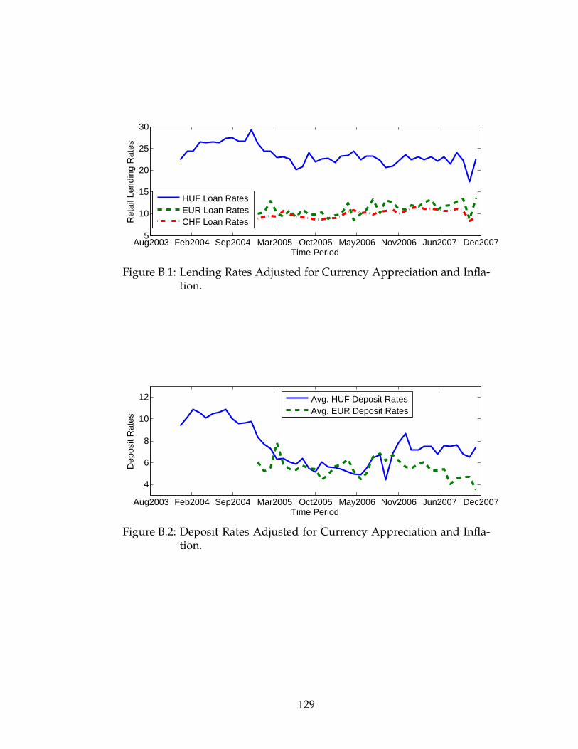
Aug2003 Feb2004 Sep2004 Mar2005 Oct2005 May2006 Nov2006 Jun2007 Dec20075

10

15

20

25

30

Time Period

Ret

ail L

endi

ng R

ates

HUF Loan RatesEUR Loan Rates CHF Loan Rates

Figure B.1: Lending Rates Adjusted for Currency Appreciation and Infla-tion.

Aug2003 Feb2004 Sep2004 Mar2005 Oct2005 May2006 Nov2006 Jun2007 Dec2007

4

6

8

10

12

Time Period

Dep

osit

Rat

es

Avg. HUF Deposit RatesAvg. EUR Deposit Rates

Figure B.2: Deposit Rates Adjusted for Currency Appreciation and Infla-tion.

129

Aug2003 Feb2004 Sep2004 Mar2005 Oct2005 May2006 Nov2006 Jun2007 Dec2007−0.5

0

0.5

1

1.5

2

Time Period

Num

ber

of N

ew B

ranc

hes

Avg. Number ofNew Bank Branches

Figure B.3: Average Expansion of Branch Network Size Over Time.

B.3 Simulation Exercises

Feb2004 Sep2004 Mar2005 Oct2005 May2006 Nov2006 Jun2007 Dec2007145

150

155

160

165

170

Time Period

Num

ber

of O

wn

Bra

nche

s

Avg. Number of Own BranchesAvg. Number of Own Branchesat 100% Initial Rise in Setup Costs

Figure B.4: Branch Network Size and Increases in Branch Setup Costs.

130

Feb2004 Sep2004 Mar2005 Oct2005 May2006 Nov2006 Jun2007 Dec20078.2

8.3

8.4

8.5

8.6

8.7

8.8

8.9

Time Period

Net

Inte

rest

Inco

me

(Log

of M

illio

n H

UF

)

Log of Avg. Net InterestIncomeLog of Avg. NII with 100%Initial Income Increase

Figure B.5: Net Interest Income and Increases in Per Capita Consumer In-come.

Feb2004 Sep2004 Mar2005 Oct2005 May2006 Nov2006 Jun2007 Dec2007140

160

180

200

220

240

260

280

Time Period

Ow

n B

ranc

h N

etw

ork

Siz

e

Avg. Branch Network SizeAvg. Branch Network Sizewith 100% Initial Income Rise

Figure B.6: Branch Network Size and Increases in Per Capita ConsumerIncome.

131

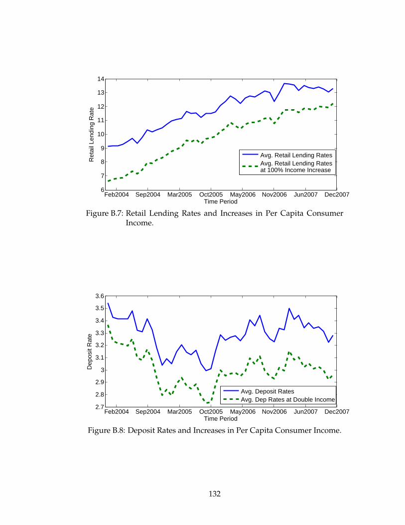
Feb2004 Sep2004 Mar2005 Oct2005 May2006 Nov2006 Jun2007 Dec20076

7

8

9

10

11

12

13

14

Time Period

Ret

ail L

endi

ng R

ate

Avg. Retail Lending RatesAvg. Retail Lending Ratesat 100% Income Increase

Figure B.7: Retail Lending Rates and Increases in Per Capita ConsumerIncome.

Feb2004 Sep2004 Mar2005 Oct2005 May2006 Nov2006 Jun2007 Dec20072.7

2.8

2.9

3

3.1

3.2

3.3

3.4

3.5

3.6

Time Period

Dep

osit

Rat

e

Avg. Deposit RatesAvg. Dep Rates at Double Income

Figure B.8: Deposit Rates and Increases in Per Capita Consumer Income.

132

Feb2004 Sep2004 Mar2005 Oct2005 May2006 Nov2006 Jun2007 Dec20070

5

10

15

20

25

30

35

40

Time Period

Mor

tgag

e R

ate

Avg. Mortgage RatesAvg. Mortgage Ratesat 100% Iinitial RiseIn Per Capita Income

Figure B.9: Mortgage Rates and Increases in Per Capita Consumer Income.

Feb2004 Sep2004 Mar2005 Oct2005 May2006 Nov2006 Jun2007 Dec20078

8.5

9

9.5

10

10.5

Time Period

Net

Inte

rest

Inco

me

(Log

Mill

ion

HU

F)

Log of Avg. Net Interest IncomeLog of Avg. NII at Double InitialCompetitors’ Branch Network Size

Figure B.10: Net Interest Income and Increases in Competitors’ BranchNetwork Size.

133

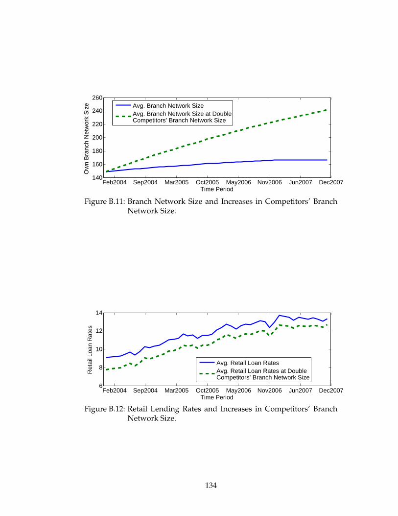
Feb2004 Sep2004 Mar2005 Oct2005 May2006 Nov2006 Jun2007 Dec2007140

160

180

200

220

240

260

Time Period

Ow

n B

ranc

h N

etw

ork

Siz

e

Avg. Branch Network SizeAvg. Branch Network Size at DoubleCompetitors’ Branch Network Size

Figure B.11: Branch Network Size and Increases in Competitors’ BranchNetwork Size.

Feb2004 Sep2004 Mar2005 Oct2005 May2006 Nov2006 Jun2007 Dec20076

8

10

12

14

Time Period

Ret

ail L

oan

Rat

es

Avg. Retail Loan RatesAvg. Retail Loan Rates at DoubleCompetitors’ Branch Network Size

Figure B.12: Retail Lending Rates and Increases in Competitors’ BranchNetwork Size.

134

Feb2004 Sep2004 Mar2005 Oct2005 May2006 Nov2006 Jun2007 Dec20072.8

3

3.2

3.4

3.6

3.8

4

Time Period

Dep

osit

Rat

e

Avg. Deposit Rates

Avg. Deposit Rates at Double InitialInitial Competitors’ Branch Network Size

Figure B.13: Deposit Rates and Increases in Competitors’ Branch NetworkSize.

Feb2004 Sep2004 Mar2005 Oct2005 May2006 Nov2006 Jun2007 Dec20070

5

10

15

20

25

Time Period

Mor

tgag

e R

ate

Avg. Mortgage RatesAvg. Mortgage Rates at Double InitialCompetitors’ Branch Network Size

Figure B.14: Mortgage Rates and Increases in Competitors’ Branch Net-work Size.

135

BIBLIOGRAPHY

ABEL, I., AND J. BONIN (2000): “Retail Banking in Hungary: A Foreign Affair?,”

William Davidson Institute Working Paper No. 356.

ABEL, I., AND P. SIKLOS (2004): “Secrets to the Successful Hungarian Bank

Privatization: The Benefits of Foreign Ownership through Strategic Partner-

ships,” Economic Systems, 28(2), 111–23.

ASLI DEMIRGUC-KUNT, A., R. LEVINE, AND H.-G. MIN (1998): “Opening to

foreign banks: Issues of stability, efficiency and growth,” in The Implications of

Globalization of World Financial Markets, ed. by S. Lee. Bank of Korea.

BAJARI, P., C. L. BENKARD, AND J. LEVIN (2007): “Estimating Dynamic Models

of Imperfect Competition,” Econometrica, 75(5), 1331–70.

BANCOGRAPHY (2003): “New Branch Survey Finds Costs Approaching $2 Mil-

lion,” Discussion Paper 8, Bancology.

BARROS, P. P. (1999): “Multimarket Competition in Banking, with an Example

from the Poruguese Market,” International Journal of Industrial Organization,

17(3), 335–52.

BARTH, J., D. E. NOLLE, AND T. N. RICE (1996): “Commercial banking struc-

ture, regulation and performance: An international comparison,” Office of

the Comptroller of the Currency Working Paper, Washington, D.C.

BASSO, H. S., O. CALVO-GONZALES, AND M. JURGILAS (2007): “Financial Dol-

larization: The Role of Banks and Interest Rates,” European Central Bank

Working Paper No. 748.

136

BAYRAKTAR, N., AND Y. WANG (2005): “Foreign bank entry and domestic

banks’ performance: evidence using bank-level data,” Penn State University

and The World Bank.

(2006): “Foreign bank entry, performance of domestic banks and the

sequence of financial liberalization,” World Bank Policy Research Working

Paper 4019.

BERGER, A., AND L. J. MESTER (2003): “Explaining the dramatic changes in

performance of US banks: technological change, deregulation, and dynamic

changes in competition,” Journal of Financial Intermediation, 12, 57–95.

BERGER, A. N., R. DEYOUNG, H. GENAY, AND G. F. UDELL (2001): “The Glob-

alization of financial institutions: Evidence from Cross-border banking per-

formance,” Federal Reserve Bank of Chicago Working Paper No. 1999–25.

BERRY, S. T., J. LEVINSOHN, AND A. PAKES (1995): “Automobile Prices in Mar-

ket Equilibrium,” Econometrica, 63, 841–90.

BUCH, C., J. C. DRISCOLL, AND C. OSTERGAARD (2005): “Cross-Border Diver-

sification in Bank Asset Portfolios,” European Central Bank Working Paper

No. 429.

CALEM, P. S., AND L. NAKAMURA (1998): “Branch Banking and the Geography

of Bank Pricing,” The Review of Economics and Statistics, 80(4), 600–10.

CAVES, R. (1987): American Industry Structure, conduct, performance. Prentice

Hall, Inc, Englewood Cliffs, NJ, 6 edn.

CERASI, V., B. CHIZZOLINI, AND M. IVALDI (2002): “Branching and Competi-

tion in the European Banking Industry,” Applied Economics, 34(17), 2213–25.

137

CERUTTI, E., G. DELL’ARICCIA, AND M. S. M. PERIA (2006): “How Banks Go

Abroad: Branches or Subsidiaries,” Journal of Banking and Finance, 31, 1669–92.

CETORELLI, N., AND L. GOLDBERG (2009): “Banking Globalization and Mone-

tary Transmission,” Federal Reserve Bank of New York Working Paper (forth-

coming in the Journal of Finance).

CHIAPPORI, P.-A., D. PEREZ-CASTRILLO, AND T. VERDIER (1995): “Spatial

Competition in the Banking System: Localization, Cross Subsidies and the

Regulation and Deposit Rates,” European Economic Review, 39(5), 889–918.

CLAESSENS, S., A. DEMIRGUC-KUNT, AND H. HUIZINGA (2000): “The Role of

foreign banks in domestic banking systems,” in The Internationalization of Fi-

nancial Services: Issues and Lessons for Developing Countries, ed. by S. Claessens,

and M. Jansen. Kluwer Academic Press, Boston, MA.

(2001): “How does foreign entry affect domestic credit markets?,” Jour-

nal of Banking and Finance, 25, 891–911.

CLAESSENS, S., AND J. LEE (2002): “Foreign banks in low income countries:

recent developments and impacts,” The World Bank.

CONDON, C. (September 19 2006): “Hungary’s PM Defies Calls to Quit,” Finan-

cial Times.

COTTARELLI, C. (1998): Hungary: Economic Policies for Sustainable Growth. . In-

ternational Monetary Fund, Washington, D.C.

DELL’ARICCIA, G. (2001): “Asymmetric Information and the Structure of the

Banking Industry,” European Economic Review, 45(10), 1957–80.

138

DEMIRGUC-KUNT, A. A., AND R. LEVINE (1996): “Stock market development

and financial intermediation,” The World Bank Economic Review, 10, 291–321.

DEMSETZ, R. S., AND P. E. STRAHAN (1995): “Diversification, Size and Risk

at Bank Holding Companies,” Federal Reserve Bank of New York Research

Paper No. 9506.

DICK, A. (2007): “Demand Estimation and Consumer Welfare in the Banking

Industry,” Journal of Banking & Finance, 32(8), 1661–76.

DUNNING, J. H. (1977): “Trade, location of economic activity and the MNE: A

search for an eclectic approach,” in The international allocation of economic activ-

ity, ed. by B. Ohlin, P. O. Hesselborn, and P. M. Wijkman, p. 395418. Macmil-

lan, London.

ECONOMIST INTELLIGENCE UNIT (1997-2005): “Country Data,”

http://www.eiu.com.

ERICSON, R., AND A. PAKES (1995): “Markov-Perfect Industry Dynamics: A

Framework for Empirical Work,” Review of Economic Studies, 62, 53–83.

ESTRADA, D., AND S. ROZO (2006): “Multimarket Spatial Competition in the

Colombian Deposit Market,” Banco de la Republica de Colombia Borradores

de Economia 413.

EWING, J. (May 6 2010): “Risky Loans In Foreign Currencies Persist In Eastern

Europe,” The New York Times.

FEDERAL FINANCIAL INSTITUTION EXAMINATION COUNCIL (1997-2005):

“Electronic Survey Data,” http://www.ffiec.gov/e16.htm.

139

FERRI, G., AND A. F. POZZOLO (2008): “Bank internationalization and trade:

What comes first?,” MoFiR Working Paper No. 11.

FOCARELLI, D., AND A. F. POZZOLO (2000): “The Determinants of Cross-Border

Bank Shareholdings: An Analysis with Bank-level Data from OECD Coun-

tries,” Bank of Italy Temi di Discussione No. 381.

(2005): “Where Do Banks Expand Abroad? An Empirical Analysis,”

Journal of Business, 78(6), 2435–64.

FREIXAS, X., AND J.-C. ROCHET (2008): Microeconomics of Banking. MIT Press,

Cambridge, MA.

FROOT, K., AND R. THALER (1990): “Anomalies: Foreign Exchange,” Journal of

Economic Perspectives, 4, 179–92.

GOLDBERG, L. (2007): “Financial Sector Foreign Direct Investment and Host

Countries: New and Old Lessons,” Economic Policy Review, 13(1), 1–17.

GOLDBERG, L., AND N. CETORELLI (2008): “Risks in U.S. Bank International

Exposures,” in Cross-Border Banking: Regulatory Challenges, ed. by G. Caprio,

D. Evanoff, and G. Kaufman. World Scientific Publishing Company, Federal

Reserve Bank of Chicago and The World Bank, Singapore.

(2009): “Globalized banks: lending to emerging markets in the crisis,”

Federal Reserve Bank of New York Staff Reports, No. 377.

GOVERNOR MARK W. OLSON, . . (2004): “Remarks at the Fortieth Annual Con-

ference on Bank Structure and Competition, Chicago, ILL.,” Sponsored by the

Federal Reserve Bank of Chicago.

140

GRAY, J. M., AND H. P. GRAY (1981): “The Multinational Bank: A Financial

MNC?,” Journal of Banking and Finance, 5(1), 33–63.

GROSSE, R., AND L. G. GOLDBERG (1991): “Foreign bank activity in the United

States: An analysis by country of origin,” Journal of Banking and Finance, 15,

1093–112.

HEINKEL, R., AND M. D. LEVI (1992): “The structure of Banking,” Journal of

International Money and Finance, 11, 251–72.

HOLLAND, B., L. COCHRANE, AND B. PENZ (October 30 2008): “’Panic’ Strikes

East Europe Borrowers as Banks Cut Franc Loans,” Bloomberg.

HOPSON, H., AND S. RYMERS (2003): “Predicting Branch Performance,” Banking

Strategies, 79(5), NA.

HOTZ, V., AND R. MILLER (1993): “Conditional Choice Probabilities and the

Estimation of Dynamic Models,” Review of Economic Studies, 60, 479–529.

HOUPT, J. V. (1999): “International Activities of U.S. Banks and in U.S. Banking

Markets,” Federal Reserve Bulletin.

HYMER, S. (1976): The International Operations of National Firms: A Study of Direct

Foreign Investment. MIT Press, Cambridge MA.

INTERNATIONAL MONETARY FUND (1997-2005): “International Financial Statis-

tics,” http://www.imfstatistics.org/imf.

IZE, A., AND E. L. YEYATI (2003): “Financial Dollarization,” Journal of Interna-

tional Economics, 59(2), 324–47.

141

KIM, M., A. LOZANO-VIVAS, AND A. MORALES (2007): “Multistrategic Spa-

tial Competition in Banking,” International Journal of the Economics of Business,

14(3), 351–66.

KIM, M., AND B. VALE (2001): “Non-pricing Strategic Behavior: The Case of

Bank Branches,” International Journal of Industrial Organization, 19(10), 1583–

1602.

KIRALY, J., AND E. VARHEGYI (2004): “Avoiding a Permanent Banking Crisis:

The Hungarian Banking Sector in the 1990s,” in Too Big To Fail: The Hazards of

Bank Bailouts, ed. by G. H. Stern, and R. Feldman. Brookings Institutions Press.

KOZPONTI STATISZTIKAI HIVATAL (2004-2007): “Statistics,”

http://www.ksh.hu.

KUHN, J. (2006): Optimal Risk-Return Trade-Offs of Commercial Banks. Springer

Verlag, Berlin.

LEVINE, R. (1999): “Foreign Bank Entry and Capital Control Liberalization: Ef-

fects on Growth and Stability,” University of Minnessota.

MAGYAR NEMZETI BANK (2004-2007): “Statistics,”

http://www.english.mnb.hu/Statisztika.

MAJNONI, G., R. SHANKAR, AND E. VARHEGYI (2003): “The Dynamics of For-

eign Bank Ownership: Evidence from Hungary,” World Bank Policy Research

Working Paper No. 3114.

MARKOWITZ, H. M. (1987): Mean-Variance Analysis in Portfolio Choice and Capital

Markets. Blackwell, New York.

142

MILLER, S., AND A. PARKHE (1998): “Patterns in the Expansion of U.S. Banks’

Foreign Operations,” Journal of International Business Studies, 29(2), 359–89.

MOLNAR, J., C. HORVATH, AND M. NAGY (2007): “A Structural Empirical

Analysis of Retail Banking Competition: the Case of Hungary,” Magyar

Nemzeti Bank Working Paper 2007 No. 1.

MORE, C., AND M. NAGY (2004): “Competition in the Hungarian Banking Mar-

ket,” Magyar Nemzeti Bank Working Paper 2004 No. 9.

NIGH, D., K. CHO, AND S. KRISHNAN (1986): “The Role of Location-related

Factors in U.S. Banking Involvement Abroad: An Empirical Examination,”

Journal of International Business Studies, Fall, 59–72.

NISHIYAMA, Y. (2007): “Are Banks Risk-averse?,” Eastern Economic Journal,

33(4), 471.

OLLEY, G. S., AND A. PAKES (1996): “The Dynamics of Productivity in the

Telecommunications Equipment Industry,” Econometrica, 64, 1263–98.

ORGANISATION FOR ECONOMIC CO-OPERATION AND DEVELOPMENT (1997-

2005): “Statistics,” http://www.stats.oecd.org.

PAKES, A., M. OSTROVSKY, AND S. BERRY. (2007): “Simple Estimators for the

Parameters of Discrete Dynamic Games (with Entry/Exit Examples),” Rand

Journal of Economics, 38, 373–99.

PAPAIOANNOU, E. (2005): “What Drives International Bank Flows? Politics, In-

stitutions, and Other Determinants,” European Central Bank Working Paper

No. 437.

143

PELLENYI, G., AND P. BILEK (2009): “Foreign Currency Borrowing: The Case of

Hungary,” Discussion paper, European Commission FINESS, FINESS Work-

ing Paper D.5.4.

PENZUGYI SZERVEZETEK ALLAMI FELUGYELETE (2004-2007): “Regulatory

Data,” http://www.pszaf.hu.

POZZOLO, F. (2008): “Bank cross-border mergers and acquisitions (Causes, con-

sequences and recent trends),” University of Molise Economics & Statistics

Discussion Paper No. 08/48.

RUUD, J. S. (2002): “U.S. Banks’ exposure to foreign financial losses,” Discus-

sion paper, Congressional Budget Office.

SABI, M. (1988): “An application of the theory of foreign direct investment to

multinational banking in LDCs,” Journal of International Business Studies, 19,

433–47.

SALOP, S. C. (1979): “Monopolistic Competition with Outside Goods,” The Bell

Journal of Economics, 10(1), 141–56.

SAUNDERS, A., AND I. WALTER (1994): Universal banking in the United States.

Oxford University Press, New York, NY.

SCHOLES, M., AND M. WOLFSON (1992): Taxes and Business Strategy: A planning

approach. Prentice Hall, Englewood Cliffs, NJ.

SHEFFIELD, C. (2006): “Branch Construction on the Upswing as Banks Counter

Growing Competition,” Memphis Business Journal.

SPIEKER, R. R. (2004): “Bank Branch Growth Has Been Steady - Will It Con-

tinue?,” Draft fob-2004-08.1., FDIC Future of Banking Study.

144

URSACKI, T., AND I. VERTINSKY. (1999): “Choice of Entry timing and scale by

foreign banks in Japan and Korea,” Journal of Banking and Finance, 16, 405–21.

VARHEGYI, E. (2004): “Bank Competition in Hungary,” Acta Oeconomica, 54(4),

403–24.

WORLD BANK (1997-2005): “Bank Regulation and Supervision,”

http://www.econ.worldbank.org.

YANNOPOULOS, G. (1983): “The growth of transnational banking,” in The

growth of international business, ed. by M. Casson. George Allen and Irwin,

London.

145