Solving disjunctive optimization

problems by generalized semi-infinite

optimization techniques∗

Peter Kirst# Oliver Stein‡

February 27, 2015

Abstract

We describe a new possibility to model disjunctive optimizationproblems as generalized semi-infinite programs. In contrast to exist-ing methods, for our approach neither a conjunctive nor a disjunctivenormal form is expected. Applying existing lower level reformulationsfor the corresponding semi-infinite program we derive conjunctive non-linear problems without any logical expressions, which can be locallysolved by standard nonlinear solvers. Our preliminary numerical re-sults on some small-scale examples indicate that our reformulationprocedure is a reasonable method to solve disjunctive optimizationproblems.

Keywords: Disjunctive optimization, generalized semi-infinite optimiza-tion, lower level duality, mathematical program with complementarity con-straints, smoothing.

AMS subject classifications: 90C34, 90C30.

Preliminary citation: Optimization Online, Preprint ID 2015-02-4795,2015.

∗This research was partially supported by the DFG (Deutsche Forschungsgemeinschaft)under grant STE 772/14-1

#Institute of Operations Research, Karlsruhe Institute of Technology (KIT), Germany,kirst@kit.edu

‡Institute of Operations Research, Karlsruhe Institute of Technology (KIT), Germany,stein@kit.edu

1

1 Introduction

In this article we describe how techniques from generalized semi-infinite op-timization may be employed to solve disjunctive optimization problems. Ageneralized semi-infinite optimization problem is defined by

GSIP : minx∈Rn

f(x) s.t. x ∈MGSIP

with the feasible set

MGSIP = x ∈ Rn| gi(x, yi) ≤ 0 for all yi ∈ Yi(x), i ∈ I.

Hence, for each index i from the finite index set I = 1, . . . , p (with p ∈ N)a set-valued mapping Yi : Rn ⇒ R

mi (with mi ∈ N, i ∈ I) describes theindex set of inequality constraints. With the so-called lower level optimalvalue functions

ϕi(x) := supyi∈Yi(x)

gi(x, yi), i ∈ I,

an obvious reformulation of the feasible set is

MGSIP = x ∈ Rn| max

i∈Iϕi(x) ≤ 0.

The functions f and gi, i ∈ I, are assumed to be at least continuous on theirrespective domains. In this article we shall assume that also the index setmappings are given in functional form as

Yi(x) = yi ∈ Rmi | vi(x, yi) ≤ 0

with at least continuous functions vi : Rn × Rmi → R

si for si ∈ N, i ∈ I.

If all set-valued mappings Yi, i ∈ I, are constant, the resulting problemis called a standard semi-infinite optimization problem (SIP). As basic ref-erences we mention [16] for an introduction to semi-infinite optimization,[17, 28] for numerical methods in SIP, and the monographs [12] for linearsemi-infinite optimization as well as [25] for algorithmic aspects. The mono-graph [31] contains a detailed study of generalized semi-infinite optimiza-tion. The most recent comprehensive reviews on theory, applications andnumerical methods of standard and generalized semi-infinite optimizationare [15, 23, 32].

Generalized semi-infinite programs turn out to be much harder to solve thanstandard semi-infinite programs although they seem to be only a slight ex-tension of the standard semi-infinite case at first glance. This is mainly due

2

to two stable properties that are neither known from finite nor from standardsemi-infinite optimization. Firstly, the feasible set of a GSIP does not needto be closed although all defining functions are continuous. Secondly, thefeasible set of a GSIP may possess so-called re-entrant corner points, that is,the feasible set may locally be expressed as the union of finitely many setswith smooth boundaries. The main idea of the present article is to exploitthis intrinsic disjunctive structure of GSIPs for the solution of disjunctiveoptimization problems.

By a disjunctive optimization problem we mean a problem of the type

DP : minx∈Rn

f(x) s.t. x ∈MDP

whose feasible set MDP is described by finitely many constraints of the formGℓ(x) ≤ 0, 1 ≤ ℓ ≤ m (with m ∈ N), which are connected by finitely manyconjunctions and disjunctions, and where the functions Gℓ, 1 ≤ ℓ ≤ m, areat least continuous. More precisely, we put

MDP = x ∈ Rn| Ω(G1(x) ≤ 0, . . . , Gm(x) ≤ 0 ) = true .

with a logical expression Ω : true, falsem → true, false consisting of onlyconjunctions and disjunctions. Due to the associativity of both, conjunctionand disjunction, we may assume that each node of the expression tree TΩ ofΩ either corresponds to

• a conjunction∧

j∈J Aj where the Aj, j ∈ J , are either disjunctions orsimple terms of the form Gℓ(x) ≤ 0 for some ℓ ∈ 1, . . . ,m, or

• a disjunction∨

j∈J Aj where the Aj, j ∈ J , are either conjunctions orsimple terms of the form Gℓ(x) ≤ 0 for some ℓ ∈ 1, . . . ,m.

For convenience, conjunctions and disjunctions of length |J | shall be called|J |−conjunctions and |J |−disjunctions, respectively. For formal reasons whichwill become apparent below, we allow 1−conjunctions and 1−disjunctions inΩ, that is, we put

∧j∈1Aj = A1 and

∨j∈1Aj = A1. Depending on

whether the root node of TΩ is a conjunction or a disjunction, we shall callTΩ a conjunction tree or a disjunction tree, respectively. Note that the levelsof TΩ alternatingly correspond to conjunctions and disjunctions, and thatthe simple terms of the form Gℓ(x) ≤ 0, ℓ ∈ 1, . . . ,m, correspond to theleafs of TΩ. By the height hΩ of TΩ we shall mean the number of edges onthe longest downward path between the root and a leaf.

3

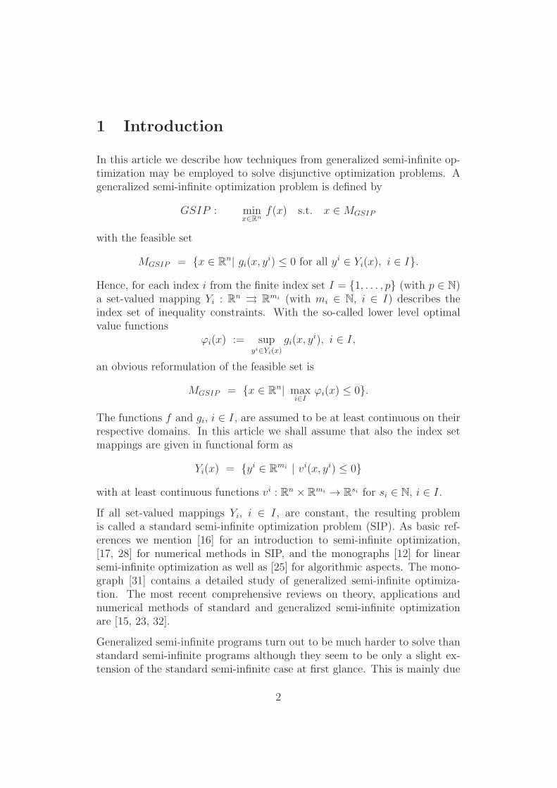
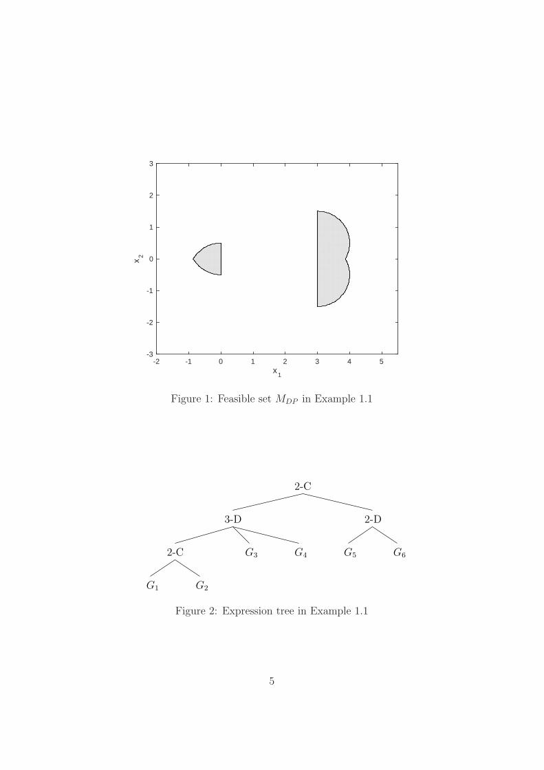
Example 1.1. Consider the problem

DP : minx∈R2

f(x) s.t. x ∈MDP

with

MDP =x ∈ R

2∣∣∣((G1(x) ≤ 0 ∧G2(x) ≤ 0

)∨G3(x) ≤ 0 ∨G4(x) ≤ 0

)

∧(G5(x) ≤ 0 ∨G6(x) ≤ 0)

)

and

f(x) := −x1G1(x) := x21 + (x2 −

1

2)2 − 1

G2(x) := x21 + (x2 +1

2)2 − 1

G3(x) := (x1 − 3)2 + (x2 −1

2)2 − 1

G4(x) := (x1 − 3)2 + (x2 +1

2)2 − 1

G5(x) := x1

G6(x) := −x1 + 3.

The set MDP is illustrated in Figure 1.

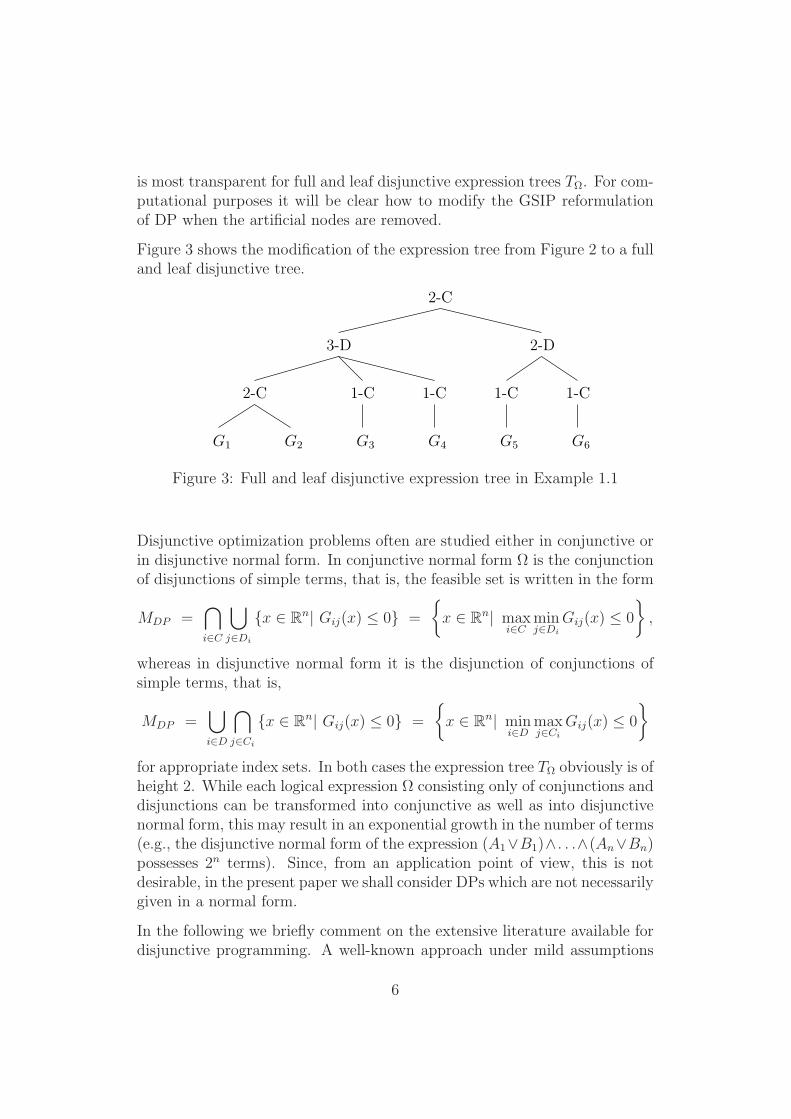
The expression tree TΩ of Ω, a conjunction tree of height hΩ = 3, is de-picted in Figure 2, where k-C stands for a k−conjunction, and k-D for ak−disjunction.

Since our proposal for a GSIP reformulation of DP in Section 2 will hingeon the structure of the expression tree for Ω, ‘nicely structured’ expressiontrees will result in a clear structure of the GSIP. For this clarity reason, wewill assume that the expression tree TΩ is full in the sense that all its leafnodes possess the same depth, that is, the number of edges between the rootand each leaf node equals the tree height hΩ. We also assume that TΩ isleaf disjunctive, by which we mean that the level of leafs corresponds to adisjunction level in TΩ.

These two assumptions may always be achieved by artificially introducing1−conjunctions and 1−disjunctions into Ω. We emphasize that, from a com-putational point of view, this is not desirable, but that our modeling approach

4

x1

-2 -1 0 1 2 3 4 5

x2

-3

-2

-1

0

1

2

3

Figure 1: Feasible set MDP in Example 1.1

G1 G2

2-C G3 G4 G5 G6

2-D3-D

2-C

Figure 2: Expression tree in Example 1.1

5

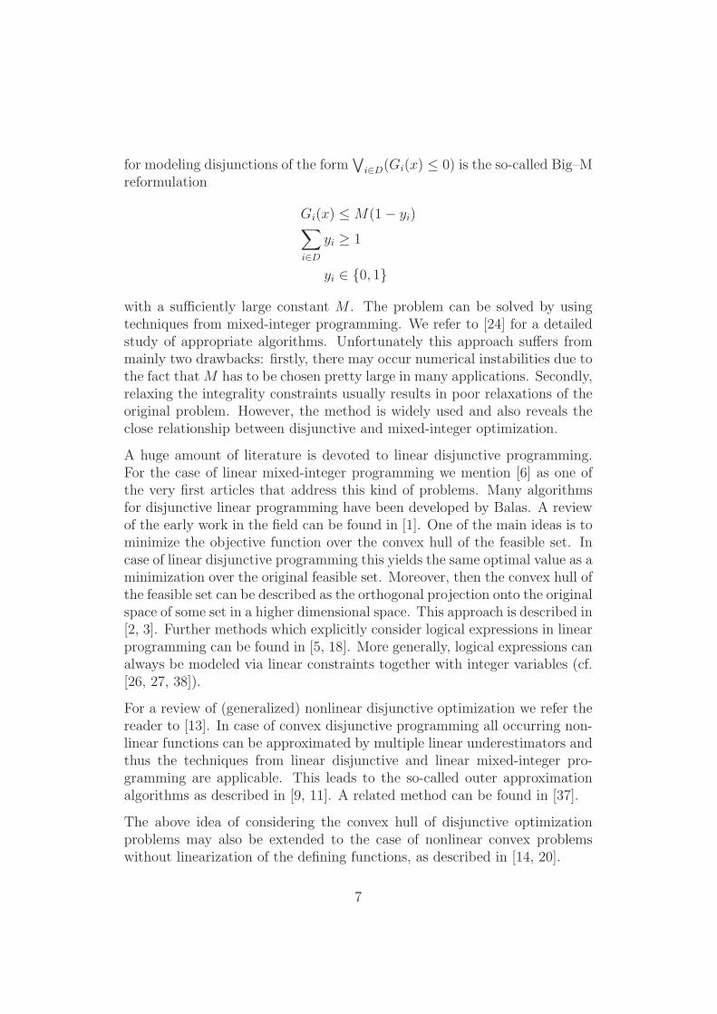
is most transparent for full and leaf disjunctive expression trees TΩ. For com-putational purposes it will be clear how to modify the GSIP reformulationof DP when the artificial nodes are removed.

Figure 3 shows the modification of the expression tree from Figure 2 to a fulland leaf disjunctive tree.

G1 G2

2-C

2-D3-D

2-C

G3 G4 G5 G6

1-C 1-C 1-C 1-C

Figure 3: Full and leaf disjunctive expression tree in Example 1.1

Disjunctive optimization problems often are studied either in conjunctive orin disjunctive normal form. In conjunctive normal form Ω is the conjunctionof disjunctions of simple terms, that is, the feasible set is written in the form

MDP =⋂

i∈C

⋃

j∈Di

x ∈ Rn| Gij(x) ≤ 0 =

x ∈ R

n| maxi∈C

minj∈Di

Gij(x) ≤ 0

,

whereas in disjunctive normal form it is the disjunction of conjunctions ofsimple terms, that is,

MDP =⋃

i∈D

⋂

j∈Ci

x ∈ Rn| Gij(x) ≤ 0 =

x ∈ R

n| mini∈D

maxj∈Ci

Gij(x) ≤ 0

for appropriate index sets. In both cases the expression tree TΩ obviously is ofheight 2. While each logical expression Ω consisting only of conjunctions anddisjunctions can be transformed into conjunctive as well as into disjunctivenormal form, this may result in an exponential growth in the number of terms(e.g., the disjunctive normal form of the expression (A1∨B1)∧ . . .∧(An∨Bn)possesses 2n terms). Since, from an application point of view, this is notdesirable, in the present paper we shall consider DPs which are not necessarilygiven in a normal form.

In the following we briefly comment on the extensive literature available fordisjunctive programming. A well-known approach under mild assumptions

6

for modeling disjunctions of the form∨

i∈D(Gi(x) ≤ 0) is the so-called Big–Mreformulation

Gi(x) ≤M(1− yi)∑

i∈Dyi ≥ 1

yi ∈ 0, 1

with a sufficiently large constant M . The problem can be solved by usingtechniques from mixed-integer programming. We refer to [24] for a detailedstudy of appropriate algorithms. Unfortunately this approach suffers frommainly two drawbacks: firstly, there may occur numerical instabilities due tothe fact thatM has to be chosen pretty large in many applications. Secondly,relaxing the integrality constraints usually results in poor relaxations of theoriginal problem. However, the method is widely used and also reveals theclose relationship between disjunctive and mixed-integer optimization.

A huge amount of literature is devoted to linear disjunctive programming.For the case of linear mixed-integer programming we mention [6] as one ofthe very first articles that address this kind of problems. Many algorithmsfor disjunctive linear programming have been developed by Balas. A reviewof the early work in the field can be found in [1]. One of the main ideas is tominimize the objective function over the convex hull of the feasible set. Incase of linear disjunctive programming this yields the same optimal value as aminimization over the original feasible set. Moreover, then the convex hull ofthe feasible set can be described as the orthogonal projection onto the originalspace of some set in a higher dimensional space. This approach is described in[2, 3]. Further methods which explicitly consider logical expressions in linearprogramming can be found in [5, 18]. More generally, logical expressions canalways be modeled via linear constraints together with integer variables (cf.[26, 27, 38]).

For a review of (generalized) nonlinear disjunctive optimization we refer thereader to [13]. In case of convex disjunctive programming all occurring non-linear functions can be approximated by multiple linear underestimators andthus the techniques from linear disjunctive and linear mixed-integer pro-gramming are applicable. This leads to the so-called outer approximationalgorithms as described in [9, 11]. A related method can be found in [37].

The above idea of considering the convex hull of disjunctive optimizationproblems may also be extended to the case of nonlinear convex problemswithout linearization of the defining functions, as described in [14, 20].

7

A critical point theory for nonlinear disjunctive optimization problems inconjunctive normal form with differentiable but not necessarily convex defin-ing functions was developed in [19].

In case of nonconvex problems in principle all branch-and-bound algorithmsfrom global optimization are applicable via the mixed-integer reformulation.We mention [21] as an example because in this branch-and-bound algorithmlogical expressions are considered explicitly.

The present article is structured as follows. Section 2 describes how disjunc-tive problems can be reformulated as generalized semi-infinite optimizationproblems. We start by considering problems in disjunctive and conjunctivenormal form. Then the ideas are extended to handle disjunctive problemswith arbitrary logical expressions. The resulting GSIPs are treated by twosolution techniques: the lower level duality reformulation in Section 3.1, andreplacing the lower level problem by its Karush-Kuhn-Tucker optimality con-ditions combined with smoothing of the resulting mathematical program withcomplementarity constraints in Section 3.2. In any case we obtain standardnonlinear optimization problems without any logical expressions, which canbe solved at least locally by common NLP-solvers. In Section 4 we performcomputational tests on some small examples. Section 5 concludes the articlewith final remarks.

2 GSIP reformulations of DPs

For disjunctive optimization problems in conjunctive normal form a GSIPreformulation is well-known from [31]. In fact, for

MDP =⋂

i∈C

⋃

j∈Di

x ∈ Rn| Gij(x) ≤ 0

with finite index sets C and Di, i ∈ C, we put p = |C|, mi = 1, gi(x, yi) = yi,

and vi(x, yi) = (yi −Gi1(x), . . . , yi −Gi,|Di|(x))

⊺, i ∈ C. Then for each i ∈ Cand x ∈ R

n the index set Yi(x) is one-dimensional and can explicitly bewritten as

Yi(x) = (−∞,minj∈Di

Gij(x) ].

Hence we obtain ϕi(x) = minj∈DiGij(x),

MGSIP = x ∈ Rn| 0 ≥ max

i∈Cϕi(x) = max

i∈Cminj∈Di

Gij(x)

and, thus, the following result.

8

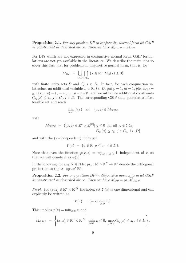
Proposition 2.1. For any problem DP in conjunctive normal form let GSIPbe constructed as described above. Then we have MGSIP =MDP .

For DPs which are not expressed in conjunctive normal form, GSIP formu-lations are not yet available in the literature. We describe the main idea tocover this case first for problems in disjunctive normal form, that is, for

MDP =⋃

i∈D

⋂

j∈Ci

x ∈ Rn| Gij(x) ≤ 0

with finite index sets D and Ci, i ∈ D. In fact, for each conjunction weintroduce an additional variable zi ∈ R, i ∈ D, put p = 1, m = 1, g(x, z, y) =y, v(x, z, y) = (y− z1, . . . , y− z|D|)

⊺, and we introduce additional constraintsGij(x) ≤ zi, j ∈ Ci, i ∈ D. The corresponding GSIP then possesses a liftedfeasible set and reads

minx,z

f(x) s.t. (x, z) ∈ MGSIP

with

MGSIP = (x, z) ∈ Rn × R

|D|| y ≤ 0 for all y ∈ Y (z)

Gij(x) ≤ zi, j ∈ Ci, i ∈ D

and with the (x−independent) index set

Y (z) = y ∈ R| y ≤ zi, i ∈ D.

Note that even the function ϕ(x, z) = supy∈Y (z) y is independent of x, sothat we will denote it as ϕ(z).

In the following, for any N ∈ N let prx : Rn×RN → R

n denote the orthogonalprojection to the ‘x−space’ Rn.

Proposition 2.2. For any problem DP in disjunctive normal form let GSIPbe constructed as described above. Then we have MDP = prxMGSIP .

Proof. For (x, z) ∈ Rn ×R

|D| the index set Y (z) is one-dimensional and canexplicitly be written as

Y (z) = (−∞,mini∈D

zi ].

This implies ϕ(z) = mini∈D zi and

MGSIP =

(x, z) ∈ R

n × R|D|

∣∣∣∣∣ mini∈D

zi ≤ 0, maxj∈Ci

Gij(x) ≤ zi , i ∈ D

.

9

Hence, for each x ∈ prxMGSIP there exist some z ∈ R|D| and some i ∈ D

with zi ≤ 0 and maxj∈CiGij(x) ≤ zi. This implies mini∈D maxj∈Ci

Gij(x) ≤ 0

and, thus, prxMGSIP ⊆MDP .

On the other hand, for each x ∈MDP we may set zi = maxj∈CiGij(x), i ∈ D,

and immediately obtain (x, z) ∈ MGSIP and, thus, MDP ⊆ prxMGSIP .

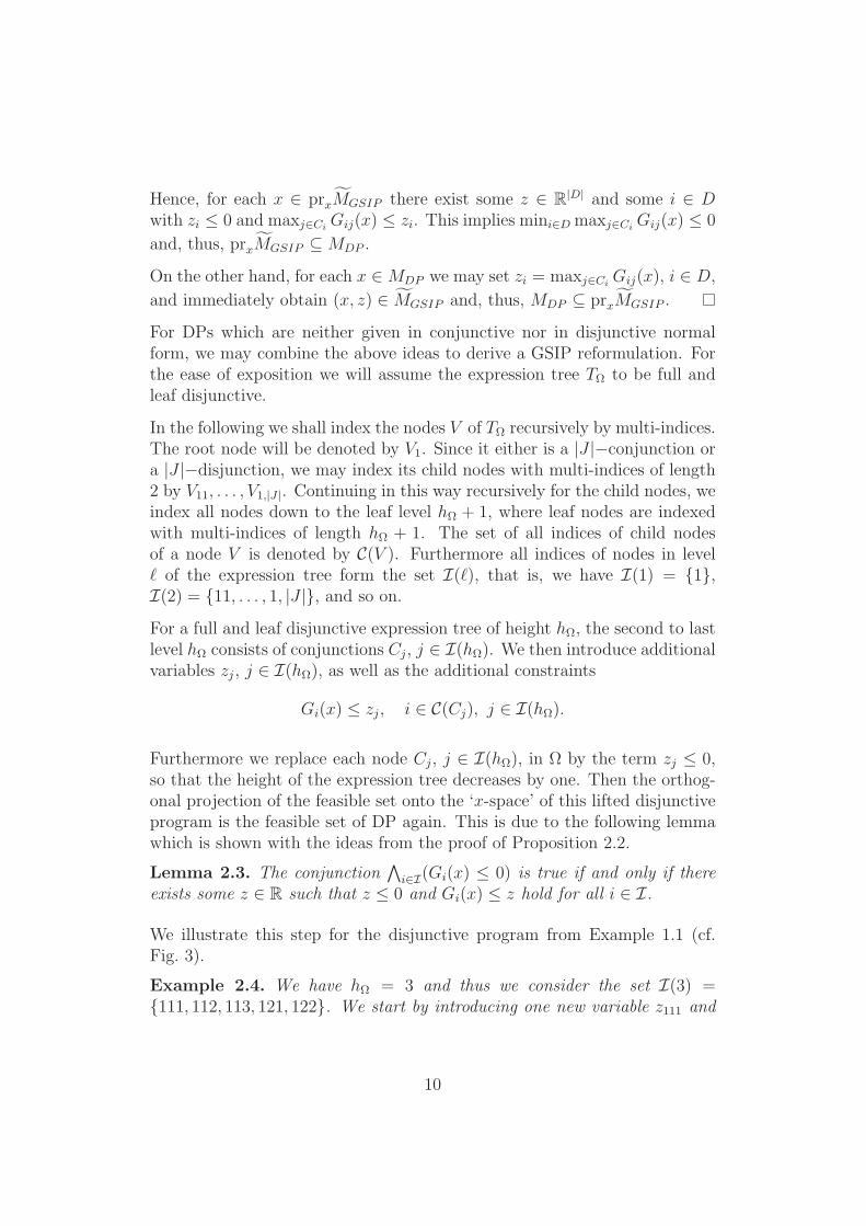
For DPs which are neither given in conjunctive nor in disjunctive normalform, we may combine the above ideas to derive a GSIP reformulation. Forthe ease of exposition we will assume the expression tree TΩ to be full andleaf disjunctive.

In the following we shall index the nodes V of TΩ recursively by multi-indices.The root node will be denoted by V1. Since it either is a |J |−conjunction ora |J |−disjunction, we may index its child nodes with multi-indices of length2 by V11, . . . , V1,|J |. Continuing in this way recursively for the child nodes, weindex all nodes down to the leaf level hΩ + 1, where leaf nodes are indexedwith multi-indices of length hΩ + 1. The set of all indices of child nodesof a node V is denoted by C(V ). Furthermore all indices of nodes in levelℓ of the expression tree form the set I(ℓ), that is, we have I(1) = 1,I(2) = 11, . . . , 1, |J |, and so on.

For a full and leaf disjunctive expression tree of height hΩ, the second to lastlevel hΩ consists of conjunctions Cj, j ∈ I(hΩ). We then introduce additionalvariables zj, j ∈ I(hΩ), as well as the additional constraints

Gi(x) ≤ zj, i ∈ C(Cj), j ∈ I(hΩ).

Furthermore we replace each node Cj, j ∈ I(hΩ), in Ω by the term zj ≤ 0,so that the height of the expression tree decreases by one. Then the orthog-onal projection of the feasible set onto the ‘x-space’ of this lifted disjunctiveprogram is the feasible set of DP again. This is due to the following lemmawhich is shown with the ideas from the proof of Proposition 2.2.

Lemma 2.3. The conjunction∧

i∈I(Gi(x) ≤ 0) is true if and only if thereexists some z ∈ R such that z ≤ 0 and Gi(x) ≤ z hold for all i ∈ I.

We illustrate this step for the disjunctive program from Example 1.1 (cf.Fig. 3).

Example 2.4. We have hΩ = 3 and thus we consider the set I(3) =111, 112, 113, 121, 122. We start by introducing one new variable z111 and

10

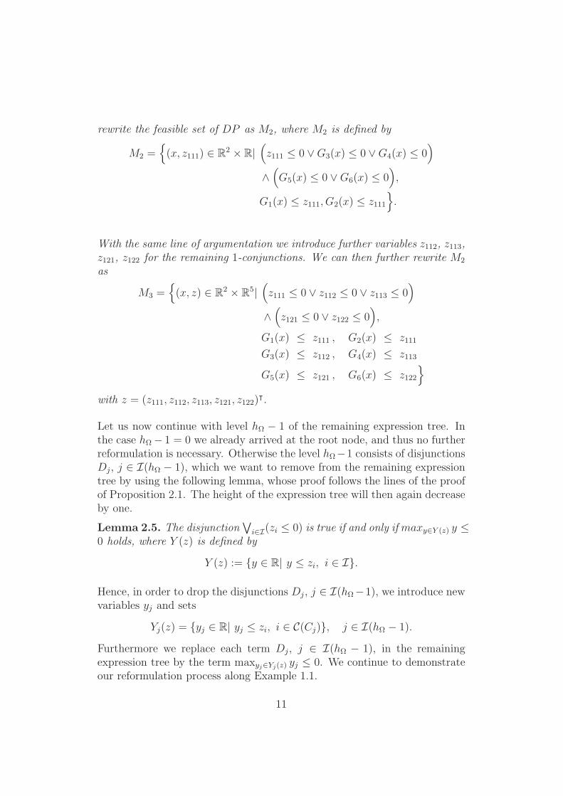
rewrite the feasible set of DP as M2, where M2 is defined by

M2 =(x, z111) ∈ R

2 × R|(z111 ≤ 0 ∨G3(x) ≤ 0 ∨G4(x) ≤ 0

)

∧(G5(x) ≤ 0 ∨G6(x) ≤ 0

),

G1(x) ≤ z111, G2(x) ≤ z111

.

With the same line of argumentation we introduce further variables z112, z113,z121, z122 for the remaining 1-conjunctions. We can then further rewrite M2

as

M3 =(x, z) ∈ R

2 × R5|(z111 ≤ 0 ∨ z112 ≤ 0 ∨ z113 ≤ 0

)

∧(z121 ≤ 0 ∨ z122 ≤ 0

),

G1(x) ≤ z111 , G2(x) ≤ z111

G3(x) ≤ z112 , G4(x) ≤ z113

G5(x) ≤ z121 , G6(x) ≤ z122

with z = (z111, z112, z113, z121, z122)⊺.

Let us now continue with level hΩ − 1 of the remaining expression tree. Inthe case hΩ − 1 = 0 we already arrived at the root node, and thus no furtherreformulation is necessary. Otherwise the level hΩ−1 consists of disjunctionsDj, j ∈ I(hΩ − 1), which we want to remove from the remaining expressiontree by using the following lemma, whose proof follows the lines of the proofof Proposition 2.1. The height of the expression tree will then again decreaseby one.

Lemma 2.5. The disjunction∨

i∈I(zi ≤ 0) is true if and only ifmaxy∈Y (z) y ≤0 holds, where Y (z) is defined by

Y (z) := y ∈ R| y ≤ zi, i ∈ I.

Hence, in order to drop the disjunctions Dj, j ∈ I(hΩ−1), we introduce newvariables yj and sets

Yj(z) = yj ∈ R| yj ≤ zi, i ∈ C(Cj), j ∈ I(hΩ − 1).

Furthermore we replace each term Dj, j ∈ I(hΩ − 1), in the remainingexpression tree by the term maxyj∈Yj(z) yj ≤ 0. We continue to demonstrateour reformulation process along Example 1.1.

11

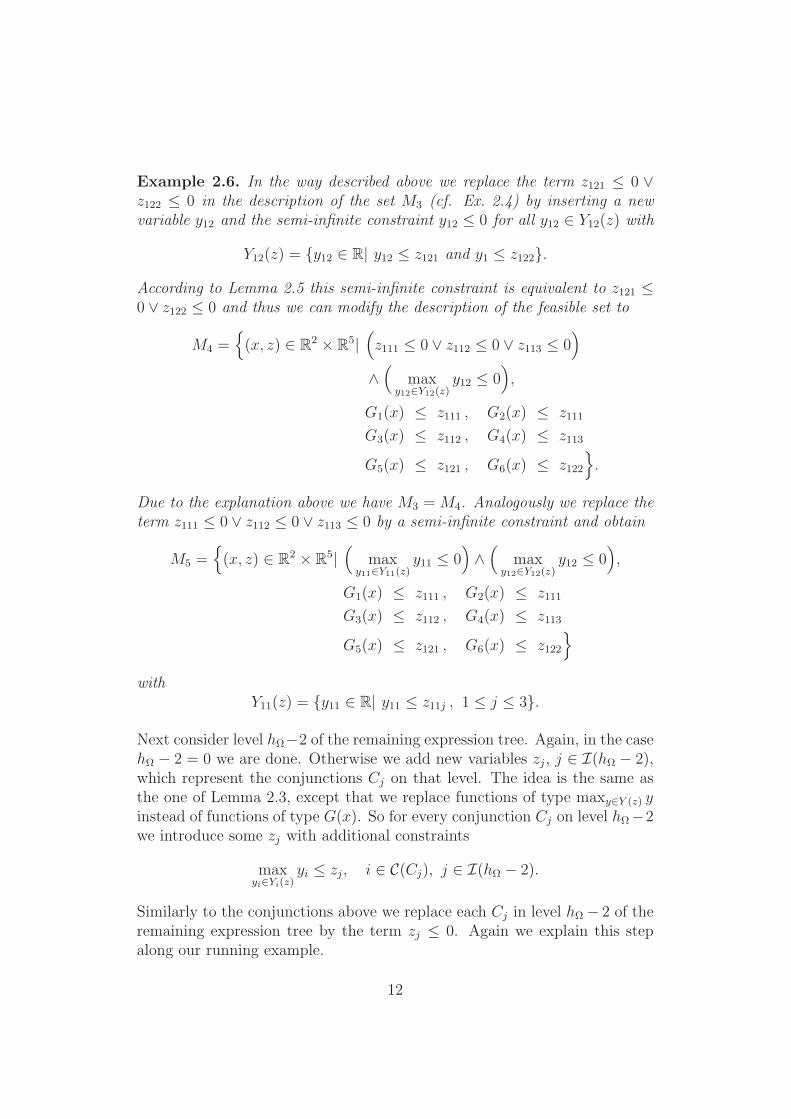
Example 2.6. In the way described above we replace the term z121 ≤ 0 ∨z122 ≤ 0 in the description of the set M3 (cf. Ex. 2.4) by inserting a newvariable y12 and the semi-infinite constraint y12 ≤ 0 for all y12 ∈ Y12(z) with

Y12(z) = y12 ∈ R| y12 ≤ z121 and y1 ≤ z122.

According to Lemma 2.5 this semi-infinite constraint is equivalent to z121 ≤0 ∨ z122 ≤ 0 and thus we can modify the description of the feasible set to

M4 =(x, z) ∈ R

2 × R5|(z111 ≤ 0 ∨ z112 ≤ 0 ∨ z113 ≤ 0

)

∧(

maxy12∈Y12(z)

y12 ≤ 0),

G1(x) ≤ z111 , G2(x) ≤ z111

G3(x) ≤ z112 , G4(x) ≤ z113

G5(x) ≤ z121 , G6(x) ≤ z122

.

Due to the explanation above we have M3 =M4. Analogously we replace theterm z111 ≤ 0 ∨ z112 ≤ 0 ∨ z113 ≤ 0 by a semi-infinite constraint and obtain

M5 =(x, z) ∈ R

2 × R5|(

maxy11∈Y11(z)

y11 ≤ 0)∧(

maxy12∈Y12(z)

y12 ≤ 0),

G1(x) ≤ z111 , G2(x) ≤ z111

G3(x) ≤ z112 , G4(x) ≤ z113

G5(x) ≤ z121 , G6(x) ≤ z122

withY11(z) = y11 ∈ R| y11 ≤ z11j , 1 ≤ j ≤ 3.

Next consider level hΩ−2 of the remaining expression tree. Again, in the casehΩ − 2 = 0 we are done. Otherwise we add new variables zj, j ∈ I(hΩ − 2),which represent the conjunctions Cj on that level. The idea is the same asthe one of Lemma 2.3, except that we replace functions of type maxy∈Y (z) yinstead of functions of type G(x). So for every conjunction Cj on level hΩ−2we introduce some zj with additional constraints

maxyi∈Yi(z)

yi ≤ zj, i ∈ C(Cj), j ∈ I(hΩ − 2).

Similarly to the conjunctions above we replace each Cj in level hΩ − 2 of theremaining expression tree by the term zj ≤ 0. Again we explain this stepalong our running example.

12

Example 2.7. We replace the term

(max

y11∈Y11(z)y11 ≤ 0

)∧(

maxy12∈Y12(z)

y12 ≤ 0)

in the description of the set M5 (cf. Ex. 2.6) by

maxy11∈Y11(z)

y11 ≤ z1 , maxy12∈Y12(z)

y12 ≤ z1 , z1 ≤ 0.

Altogether, the GSIP reformulation of this DP turns out to be

GSIP : minx,z

f(x) s.t. z1 ≤ 0, maxy11∈Y11(z)

y11 ≤ z1 , maxy12∈Y12(z)

y12 ≤ z1

G1(x) ≤ z111 , G2(x) ≤ z111

G3(x) ≤ z112 , G4(x) ≤ z113

G5(x) ≤ z121 , G6(x) ≤ z122

with the vector z = (z1, z111, z112, z113, z121, z122)⊺ and the sets Y11(z), Y12(z)

as defined above.

In this way for both, conjunctive and disjunctive, expression trees TΩ weobtain GSIP reformulations after finitely many steps. We will denote the(lifted) feasible set of the resulting GSIP by MGSIP .

Note that the variable z1 appearing in the reformulation of a conjunctivetree (as in the above example) is a mere dummy variable which may beeliminated in computations. As mentioned earlier, also variables which areonly introduced since TΩ has to be given in full and leaf disjunctive form, maybe eliminated. For example, our construction requires a tree of height three(i.e., with four levels), to model a logical expression Ω given in conjunctivenormal form. Here, not only the variable corresponding to the root node,but also all variables corresponding to 1−conjunctions in the third level maybe eliminated. In the following we shall omit further discussions of theseelimination options.

The next theorem is proved by recursively applying the Lemmata 2.3 and2.5.

Theorem 2.8. For any problem DP whose expression tree TΩ is full andleaf disjunctive, let GSIP be constructed as described above. Then we haveMDP = prxMGSIP .

13

3 GSIP solution techniques for DPs

The GSIP reformulation of DPs from Section 2 generates generalized semi-infinite constraints which all share the simple structure

ϕ(z) ≤ ζ

withϕ(z) = max

y∈Y (z)y

andY (z) = y ∈ R| y ≤ zk, 1 ≤ k ≤ s,

where the variable ζ ∈ R does not belong to the auxiliary variables listed inthe vector z ∈ R

s. Note that the original decision vector x ∈ Rn does not

explicitly appear in these generalized semi-infinite constraints, but enters viathe simple coupling constraints between the entries of z and the functionsG1, . . . , Gm (see Sec. 2).

In the following we shall describe different approaches to handle a constraintof the form ϕ(z) ≤ ζ algorithmically. The application of the respectiveapproaches to all appearing generalized semi-infinite constraints then leadsto a solution method for the original DP. We will briefly describe the mainideas of the methods before applying them to the problem at hand. For moredetails we refer to [32] and the references therein.

All subsequent approaches rely on the bilevel structure of generalized semi-infinite constraints, that is, the function ϕ is interpreted as the optimal valuefunction of the so-called lower level problem

Q(z) : maxy∈R

y s.t. y ≤ zk , 1 ≤ k ≤ s.

Since the problem Q(z) is a one-dimensional linear optimization problem, onemay expect that sophisticated GSIP techniques collapse to rather obviousapproaches. We shall see, however, that this is only partly the case.

3.1 The lower level duality reformulation

For convex lower level problems in generalized semi-infinite optimization,the idea to employ duality arguments goes back at least to [22] (for convex-quadratic problems). Similar approaches have been used in robust optimiza-tion and lead to a systematic treatment of GSIPs with smooth convex lower

14

level problems in [8]. There, the function ϕ is rewritten as the optimal valuefunction of the corresponding Wolfe dual of the lower level problem, and theadditional dual variables are included by lifting the feasible set.

In the present setting of the above problem Q(z), this approach of coursecollapses to standard linear programming duality. The dual problem is

D(z) : minγ∈Rs

γ⊺z s.t. γ ∈ Σ

with the standard simplex

Σ = γ ∈ Rs| γ ≥ 0, e⊺γ = 1

and the all-ones vector e. In view of strong duality we may rewrite the GSIPconstraint as

ζ ≥ ϕ(z) = minγ∈Σ

γ⊺z,

or, equivalently, as

∃ γ ∈ Rs : γ ≥ 0, e⊺γ = 1, γ⊺z ≤ ζ.

Replacing each generalized semi-infinite constraint by this construction andlifting the feasible set to the corresponding set MP transforms the GSIP re-formulation of DP into a finite and purely conjunctive optimization problem.

Example 3.1. The lower level duality reformulation for the GSIP formula-tion of the DP from Example 1.1 in Example 2.7 is constructed as follows.Since the index set

Y11(z) = y11 ∈ R| y11 ≤ z11j , 1 ≤ j ≤ 3

is described by three constraints, we introduce the vector ~γ11 = (γ111, γ112, γ113)⊺ ∈

R3 and may rewrite the constraint

maxy11∈Y11(z)

y11 ≤ z1

as

∃~γ11 ∈ R3 : ~γ11 ≥ 0, e⊺~γ11 = 1, γ111 z111 + γ112 z112 + γ113 z113 ≤ z1.

Analogously, we replace the constraint

maxy12∈Y12(z)

y12 ≤ z1

15

by∃~γ12 ∈ R

2 : ~γ12 ≥ 0, e⊺~γ12 = 1, γ121 z121 + γ122 z122 ≤ z1.

This results in the finite conjunctive optimization problem

P : minx,z,γ

f(x) s.t. z1 ≤ 0,

~γ11 ≥ 0, e⊺~γ11 = 1, γ111 z111 + γ112 z112 + γ113 z113 ≤ z1

~γ12 ≥ 0, e⊺~γ12 = 1, γ121 z121 + γ122 z122 ≤ z1

G1(x) ≤ z111 , G2(x) ≤ z111

G3(x) ≤ z112 , G4(x) ≤ z113

G5(x) ≤ z121 , G6(x) ≤ z122

with the vector z defined as in Example 2.7, and γ = (γ111, γ112, γ113, γ121, γ122)⊺.

The subsequent result follows from our above discussions.

Theorem 3.2. For any problem DP whose expression tree TΩ is full and leafdisjunctive, let the purely conjunctive problem P be constructed as describedabove. Then we have MDP = prxMP .

We emphasize that resorting to GSIP techniques would actually not be nec-essary to come up with this reformulation of DP. In fact, the vertex theo-rem of linear programming immediately implies that the discrete minimummin1≤k≤s zk may be rewritten as the continuous minimum minγ∈Σ γ

⊺z, fromwhich the presented lifting approach follows along the lines sketched above.

Either way, this reformulation approach possesses the drawback that it mayproduce spurious Karush-Kuhn-Tucker points, in which an NLP solver forthe problem P may terminate without identifying a locally minimal point ofDP . We shall illustrate this effect for a so-called re-entrant corner point ofthe disjunctive program

DP : min f(x) s.t. G1(x) ≤ 0 ∨ . . . ∨ Gn(x) ≤ 0

with continuously differentiable functions f , G1, . . . , Gn and n ≥ 2. Infact, x ∈ R

n is called a re-entrant corner point of MDP if Gi(x) = 0 holdsfor all i = 1, . . . , n, and if the gradients ∇Gi(x), i = 1, . . . , n, are linearlyindependent. In Example 1.1 the point (3 +

√3/2, 0) is a re-entrant corner

point.

After the deletion of auxiliary variables, the lifted problem P correspondingto DP is

P : minx,γ

f(x) s.t. γ⊺G(x) ≤ 0, γ⊺e = 1, γ ≥ 0.

16

Proposition 3.3. For a re-entrant corner point x of DP let there existmultipliers ¯i > 0, i = 1, . . . , n, with

∇f(x) +n∑

i=1

¯i∇Gi(x) = 0.

Then there exists a vector γ ∈ Σ such that (x, γ) is a Karush-Kuhn-Tuckerpoint of P at which the linear independence constraint qualification as wellas strict complementary slackness are satisfied.

Proof. The vector γ := ¯/‖ ¯‖1 lies in γ ∈ Σ and satisfies γ > 0, that is, noneof the constraints γi ≥ 0, i = 1, . . . , n, in P is active at (x, γ). In view ofG(x) = 0, on the other hand, the constraint γ⊺G(x) ≤ 0 is active at (x, γ).

The gradients, with respect to (x, γ), of the two active constraints are lin-early independent as the nontrivial linear combination ∇G(x)γ of the gradi-ents ∇Gi(x), i = 1, . . . , n, cannot vanish under the linear independence as-sumption at re-entrant corner points. Furthermore, the Karush-Kuhn-Tuckercondition (

∇f(x)0

)+ λ

(∇G(x)γ

0

)+ µ

(0e

)=

(00

)

of P at (x, γ) possesses the unique solution λ = ‖ ¯‖1 > 0 and µ = 0. Inparticular, also strict complementary slackness holds.

The following result shows, at least, that algorithms using second order in-formation when solving P should not terminate in a spurious Karush-Kuhn-Tucker point from Proposition 3.3, since a second order descent directionalways exists.

Proposition 3.4. In addition to the assumptions of Proposition 3.3, let thefunctions f , Gi, i = 1, . . . , n, be twice continuously differentiable. Then asecond order descent direction for P exists at (x, γ).

Proof. With the notation from the proof of Proposition 3.3 recall the relationsγ > 0 and λ > 0. Let us define the vectors

δ :=

(1, . . . , 1,−

(n−1∑

i=1

γi

)/γn

)⊺

,

d(c) := c(∇G(x))−⊺δ with c > 0,

as well asη := (−1, . . . ,−1, n− 1)⊺.

17

Then, for any c > 0, the vector (d(c), η) lies in the tangent space to thefeasible set of P at (x, γ), since we have

⟨(∇G(x)γ

0

),

(d(c)η

)⟩= c〈γ, δ〉 = 0

and ⟨(0e

),

(d(c)η

)⟩= 〈e, η〉 = 0.

Moreover, the Hessian with respect to (x, γ) of the corresponding Lagrangianof P ,

L(x, γ, λ, µ) = f(x) + λγ⊺G(x) + µ(γ⊺e− 1)

at (x, γ, λ, µ) is

D2(x,γ)L(x, γ, λ, µ) =

(D2f(x) + λ

∑n

i=1 γiD2Gi(x) λ∇G(x)

λ∇G(x)⊺ 0

),

and we obtain(d(c)η

)⊺

D2(x,γ)L(x, γ, λ, µ)

(d(c)η

)

= d(c)⊺

(D2f(x) +

n∑

i=1

¯iD2Gi(x)

)d(c) + 2λd(c)⊺∇G(x)η

= c2δ⊺∇G(x)−1

(D2f(x) +

n∑

i=1

¯iD2Gi(x)

)(∇G(x))−⊺δ

+2λcδ⊺η.

Due to λ > 0 and

δ⊺η = −(n− 1)− n− 1

γn

n−1∑

i=1

γi < 0

the latter is negative for a sufficiently small value c > 0, so that (d(c), η) isthe asserted second order descent direction.

3.2 The outer and inner smoothing reformulations

From an algorithmic point of view it is often useful to know outer and in-ner approximations of the feasible set of an optimization problem. For the

18

set MDP this section shows how smoothing methods from generalized semi-infinite optimization may be employed to this end.

In fact, for any generalized semi-infinite optimization problem of the generalform

GSIP : minx∈Rn

f(x) s.t. x ∈MGSIP

with the feasible set

MGSIP = x ∈ Rn| gi(x, yi) ≤ 0 for all yi ∈ Yi(x), i ∈ I

andYi(x) = yi ∈ R

mi | vi(x, yi) ≤ 0, i ∈ I,

in [33] the equivalence of GSIP with the problem

SG : minx,y1,...,yp

f(x) s.t. g(x, yi) ≤ 0, yi is a solution of Qi(x), i ∈ I

is shown, as long as Yi(x) is nonempty for all x ∈ Rn and i ∈ I. Here, the

lower level problem of the constraint indexed with i ∈ I is denoted by

Qi(x) : maxyi∈Yi(x)

gi(x, yi) s.t. vi(x, yi) ≤ 0.

Note that the former index variables yi, i ∈ I, are treated as additionaldecision variables in SG, so that already this step of the reformulation isa lifting approach. Since a part of the decision variables is constrained tosolve an optimization problem depending on the other decision variables, thisproblem has the structure of a Stackelberg game ([4, 7]).

In a next step, for each i ∈ I the fact that yi solves Qi(x) is equivalentlyreplaced by an optimality condition. If the problems Qi(x), i ∈ I, are convex,the Slater condition holds in each set Yi(x), x ∈ R

n, i ∈ I, and all functionsgi, v

i, i ∈ I, are continuously differentiable on their respective domains, thismay be achieved by the Karush-Kuhn-Tucker conditions

∃ γi ∈ Rsi : ∇ygi(x, y

i)−∇yvi(x, yi) γi = 0,

0 ≤ γi ⊥ −vi(x, yi) ≥ 0

for each i ∈ I, where the second line stands for a complementarity condition.The introduction of the additional variables γi, i ∈ I, leads to another lift-ing of the feasible set whose description, however, contains complementarity

19

constraints. The resulting problem is, thus, the mathematical program withcomplementarity constraints

MPCC : minx,y1,...,yp,γ1,...,γp

f(x) s.t. g(x, yi) ≤ 0,

∇ygi(x, yi)−∇yv

i(x, yi) γi = 0,

0 ≤ γi ⊥ −vi(x, yi) ≥ 0, i ∈ I.

MPCCs turn out to be numerically challenging, since the so-called Mangasa-rian-Fromovitz constraint qualification (MFCQ) is violated everywhere intheir feasible set ([30]).

A first numerical approach to the MPCC reformulation of a general GSIP wasgiven in [31, 34] by applying the smoothing procedure for MPCCs from [10].In fact, each scalar complementarity constraint 0 ≤ γik ⊥ −vik(x, yi) ≥ 0,1 ≤ k ≤ si, i ∈ I, is first replaced by the equation ψ(γik,−vik(x, yi)) = 0 witha complementarity function ψ like the natural residual function ψNR(a, b) =min(a, b) or the Fischer-Burmeister function ψFB(a, b) = a + b −

√a2 + b2.

The nonsmooth function ψ is then equipped with a smoothing parameterτ > 0, for example

ψNRτ (a, b) =

1

2

(a+ b−

√(a− b)2 + 4τ 2

)

orψFBτ (a, b) = a+ b−

√a2 + b2 + 2τ 2,

so that ψτ is smooth and ψ0 coincides with ψ. This gives rise to the familyof smoothed problems

Pτ : minx,y1,...,yp,γ1,...,γp

f(x) s.t. g(x, yi) ≤ 0,

∇ygi(x, yi)−∇yv

i(x, yi) γi = 0,

ψτ (γi,−vi(x, yi)) = 0, i ∈ I

with τ > 0, where ψτ is extended to vector arguments componentwise. Undermild assumptions, in [31, 34] it is shown that Pτ is numerically tractable, andthat stationary points of Pτ tend to a stationary point of GSIP for τ → 0.

While MPCC still is an equivalent formulation of GSIP, the smoothed prob-lem Pτ only is an approximation. In [31] it is shown that its feasible set Mτ

at least satisfies prxMτ ⊇ MGSIP , that is, it constitutes an outer approxi-mation of MGSIP for τ > 0. This means, unfortunately, that the x−parts ofoptimal points of Pτ must be expected to be infeasible for GSIP.

20

However, in [35] it could be shown that a simple modification of Pτ leads toinner approximations of MGSIP and, thus, to feasible optimal points of theapproximating problems. In fact, an error analysis for the approximation ofthe lower level optimal value proves that the feasible set M

τ of

P τ : min

x,y1,...,yp,γ1,...,γpf(x) s.t. g(x, yi) + siτ

2 ≤ 0,

∇ygi(x, yi)−∇yv

i(x, yi) γi = 0,

ψτ (γi,−vi(x, yi)) = 0, i ∈ I

satisfies prxMτ ⊆MGSIP (where si denotes the number of lower level inequal-

ity constraints). A combination of the outer and inner smoothing approachesleads to ‘sandwiching’ procedures for MGSIP (cf. [35]).

For each lower level problem of the form

Q(z) : maxy∈R

y s.t. y ≤ zk , 1 ≤ k ≤ s

appearing in the GSIP reformulation of DPs, the convexity and differentia-bility assumptions as well as the Slater condition are obviously satisfied, sothat outer smoothing is achieved by the constraints

y ≤ 0, e⊺γ = 1, ψτ (γk , zk − y) = 0, 1 ≤ k ≤ s,

whereas inner smoothing results from

y + sτ 2 ≤ 0, e⊺γ = 1, ψτ (γk , zk − y) = 0, 1 ≤ k ≤ s.

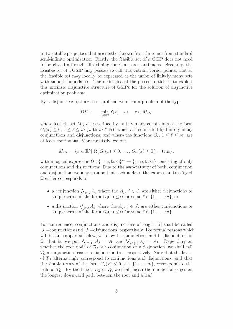
Example 3.5. We construct the outer smoothing reformulation for the GSIPformulation of the DP from Example 1.1 in Example 2.7 as follows. For theindex set

Y11(z) = y11 ∈ R| y11 ≤ z11j , 1 ≤ j ≤ 3we again introduce the vector ~γ11 ∈ R

3, but now subject to the constraints

y11 ≤ z1, e⊺~γ11 = 1, ψτ (γ11j , z11j − y11) = 0, 1 ≤ j ≤ 3

with some τ > 0. An analogous construction for the second generalized semi-infinite constraint leads to the finite conjunctive optimization problem

Pτ : minx,y,z,γ

f(x) s.t. z1 ≤ 0

y11 ≤ z1, e⊺~γ11 = 1, ψτ (γ11j, z11j − y11) = 0, 1 ≤ j ≤ 3

y12 ≤ z1, e⊺~γ12 = 1, ψτ (γ12j, z12j − y12) = 0, 1 ≤ j ≤ 2

G1(x) ≤ z111 , G2(x) ≤ z111

G3(x) ≤ z112 , G4(x) ≤ z113

G5(x) ≤ z121 , G6(x) ≤ z122

21

with y = (y11, y12)⊺ and the vectors z and γ defined as in Examples 2.7 and

3.1.

The inner smoothing problem, on the other hand, is given by

P τ : min

x,y,z,γf(x) s.t. z1 ≤ 0

y11 + 3τ 2 ≤ z1, e⊺~γ11 = 1, ψτ (γ11j, z11j − y11) = 0, 1 ≤ j ≤ 3

y12 + 2τ 2 ≤ z1, e⊺~γ12 = 1, ψτ (γ12j, z12j − y12) = 0, 1 ≤ j ≤ 2

G1(x) ≤ z111 , G2(x) ≤ z111

G3(x) ≤ z112 , G4(x) ≤ z113

G5(x) ≤ z121 , G6(x) ≤ z122 .

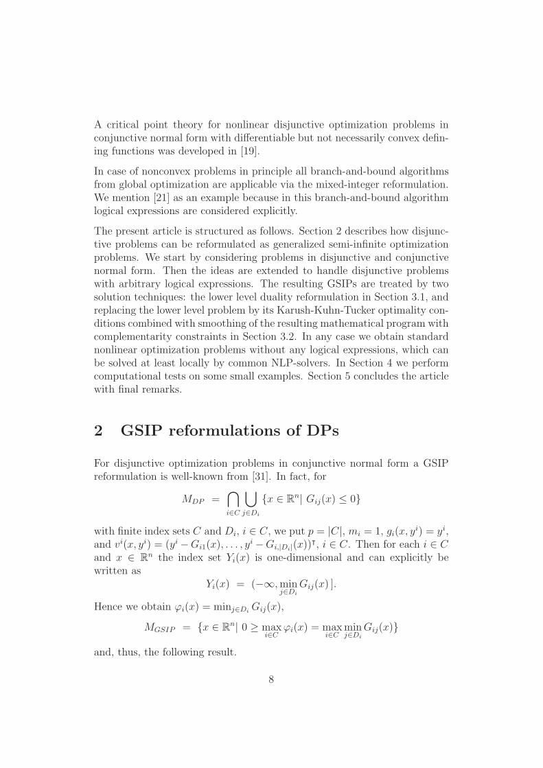
Figure 4 shows the projected feasible sets resulting from outer and innersmoothings for the set MDP from Figure 1, for several values of τ .

x1

-2 -1 0 1 2 3 4 5

x2

-3

-2

-1

0

1

2

3

Figure 4: Outer and inner smoothings from Example 3.5

We summarize our discussion in the following result.

Theorem 3.6. For any problem DP whose expression tree TΩ is full andleaf disjunctive, let the purely conjunctive smoothing problems Pτ and P

τ be

constructed as described above. Then we have prxMτ ⊆MDP ⊆ prxMτ .

22

Unfortunately, smoothing does not prevent the appearance of the spuri-ous Karush-Kuhn-Tucker points from Section 3.1. This is a consequenceof typical nondegeneracy of spurious Karush-Kuhn-Tucker points in the un-perturbed problem P and the implicit function theorem. In fact, theseKarush-Kuhn-Tucker points then prevail under small perturbations, andsmall smoothing parameters τ > 0 may be interpreted as such perturba-tions. We omit the details of this analysis for space reasons.

4 Preliminary numerical results

In this section we present our numerical results. Our computational tests areperformed on a Intel Pentium CPU 987, 1.5 GHz with 4 GB of RAM runningLinux. As a solver for the occurring nonlinear problems we used Ipopt [36],version 3.11.7. The termination tolerance is set to 10−6. The algorithm isimplemented in C++ and compiled with GNU g++, version 4.7.

In the largest part of our implementation we make heavy use of operatoroverloading to construct the conjunctive optimization problem based on thegiven disjunctive problem. This makes it is pretty convenient to model evencomplex logical expressions since both, the lower level duality reformulationas well as the outer and inner smoothing reformulations, can be constructedautomatically.

However, no automatic or numerical differentiation is implemented and thusthe first derivatives have to be entered manually so far. All Hessians areapproximated using a feature of Ipopt.

For the test problem

DP : minx∈R2

f(x) s.t. x ∈MDP

withMDP =

x ∈ R

2∣∣∣(G1(x) ≤ 0 ∨G2(x) ≤ 0

)∧G3(x) ≤ 0

and

f(x) := −x2G1(x) := x21 + x22 − 1

G2(x) := (x1 − 1)2 + x22 − 1

G3(x) := −x2

23

the feasible set can be described as the union of two semi discs, both withradius 1. Their midpoints are the origin and (1, 0)⊺, respectively, and theglobally minimal points of the problem are (0, 1)⊺ and (1, 1)⊺. There are nofurther locally minimal points, while we do have a re-entrant corner point at(0.5,

√32)⊺ that leads to a spurious Karush-Kuhn-Tucker point in the lower

level duality reformulation as described in Section 3.

Using the lower level duality reformulation and starting Ipopt from the point(x01, x

02, 0, . . . , 0)

⊺ with (x01, x02) = (0, 0), the algorithm converges to a point

with first components (x∗1, x∗2)

⊺ = (0.00000, 1.00000)⊺, which corresponds toone of the globally minimal points of the original problem, within 10 itera-tions. We obtained very similar results for various different starting points ofthe form (x01, x

02, 0, . . . , 0)

⊺ where x01 and x02 are chosen from the set −1, 0, 1.

The algorithm then always converges to one of the globally minimal points.The results are presented in the upper part of Table 1 where (x01, x

02) denotes

the first to coordinates for the initial point, (x∗1, x∗2) denotes the first coordi-

nates of the limit point computed by the nonlinear solver and v∗ is the valueof the objective function at that point.

There seems to be one notable exception to this observation that we showin the lower part of Table 1. If in the initial point we set x01 = 0.5, x02 ∈ R,and the remaining variables to zero, the algorithm is likely to converge tothe spurious Karush-Kuhn-Tucker point mentioned above. This even holdsfor more points with x01 = 0.5, but not for all as can be seen from the verylast row. This is in accordance with Proposition 3.4 which guarantees theexistence of a second order descent direction at the spurious KKT pointand, thus, convergence to this point at most along some lower dimensionalmanifold.

In principle the numerical observations from the paragraph above remaintrue if we switch from the lower level duality reformulation to the smoothedmathematical program with complementarity constraints. This can be seenfrom Table 2 and Table 3. With τ = 0.1 the smoothing parameter is chosenpretty large to demonstrate the effects from the outer and inner approxima-tion. Starting from (0, 0, 0 . . . , 0)⊺ the algorithm converges to a point with(x∗1, x

∗2)

⊺ = (0.00010, 1.00504)⊺ within 15 iterations. For the inner approxi-mation with the same value of τ it takes 14 iterations to approximate a pointwith the first two components (x∗1, x

∗2)

⊺ = (0.00010, 0.99504)⊺. Thus, in bothcases we generate a point close to one of the globally minimal points of theoriginal problem.

There are two test runs in Table 2 and Table 3, respectively, that do not work

24

(x01, x02) (x∗1, x

∗2) v∗

(−1.0,−1.0) (0.000000, 1.000000) −1.000000(−1.0, 0.0) (0.000000, 1.000000) −1.000000(−1.0, 1.0) (0.000000, 1.000000) −1.000000(0.0,−1.0) (1.000000, 1.000000) −1.000000(0.0, 0.0) (0.000001, 1.000000) −1.000000(0.0, 1.0) (0.000000, 1.000000) −1.000000(1.0,−1.0) (0.000000, 1.000000) −1.000000(1.0, 0.0) (0.999999, 1.000000) −1.000000(1.0, 1.0) (1.000000, 1.000000) −1.000000(0.5,−2.0) (0.500000, 0.866025) −0.866025(0.5,−1.0) (0.500000, 0.866025) −0.866025(0.5, 0.0) (0.500000, 0.866025) −0.866025(0.5, 1.0) (0.500000, 0.866025) −0.866025(0.5, 2.0) (0.000000, 1.000000) −1.000000

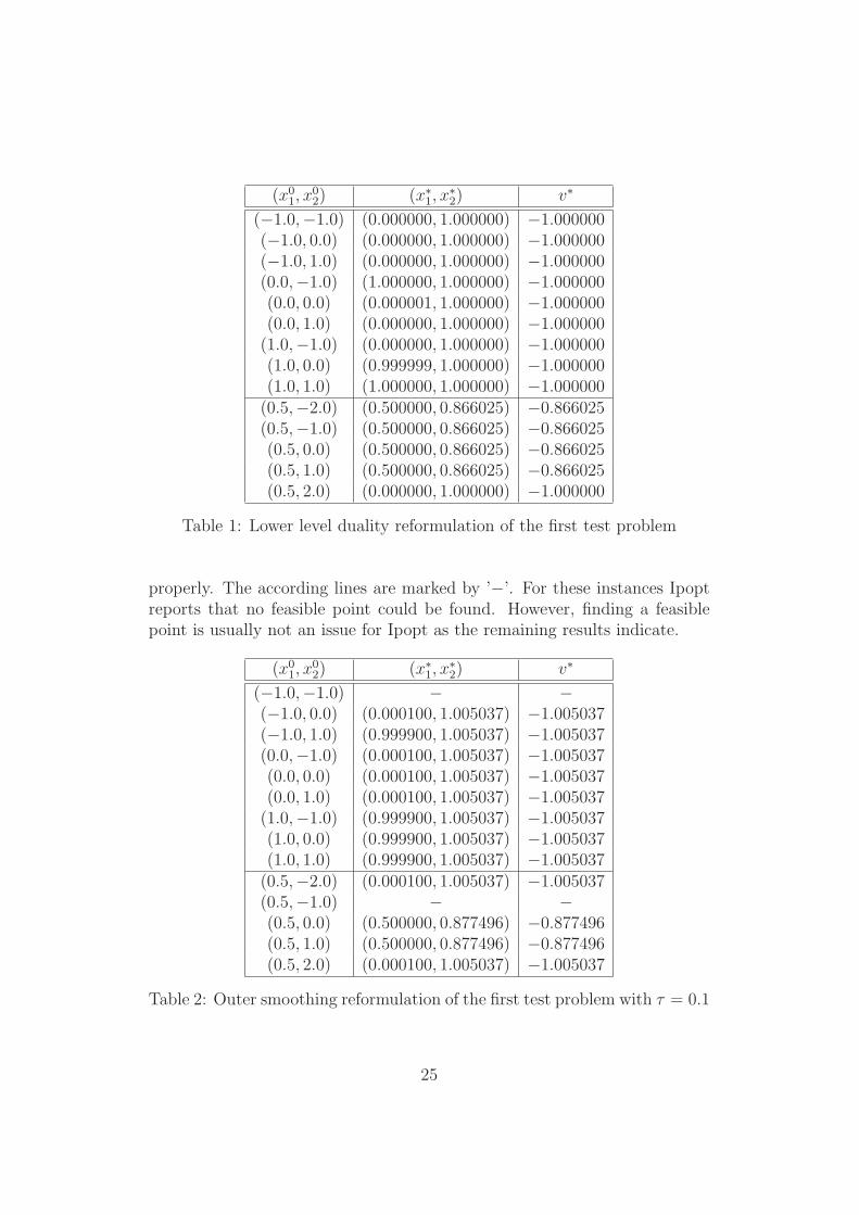
Table 1: Lower level duality reformulation of the first test problem

properly. The according lines are marked by ’−’. For these instances Ipoptreports that no feasible point could be found. However, finding a feasiblepoint is usually not an issue for Ipopt as the remaining results indicate.

(x01, x02) (x∗1, x

∗2) v∗

(−1.0,−1.0) − −(−1.0, 0.0) (0.000100, 1.005037) −1.005037(−1.0, 1.0) (0.999900, 1.005037) −1.005037(0.0,−1.0) (0.000100, 1.005037) −1.005037(0.0, 0.0) (0.000100, 1.005037) −1.005037(0.0, 1.0) (0.000100, 1.005037) −1.005037(1.0,−1.0) (0.999900, 1.005037) −1.005037(1.0, 0.0) (0.999900, 1.005037) −1.005037(1.0, 1.0) (0.999900, 1.005037) −1.005037(0.5,−2.0) (0.000100, 1.005037) −1.005037(0.5,−1.0) − −(0.5, 0.0) (0.500000, 0.877496) −0.877496(0.5, 1.0) (0.500000, 0.877496) −0.877496(0.5, 2.0) (0.000100, 1.005037) −1.005037

Table 2: Outer smoothing reformulation of the first test problem with τ = 0.1

25

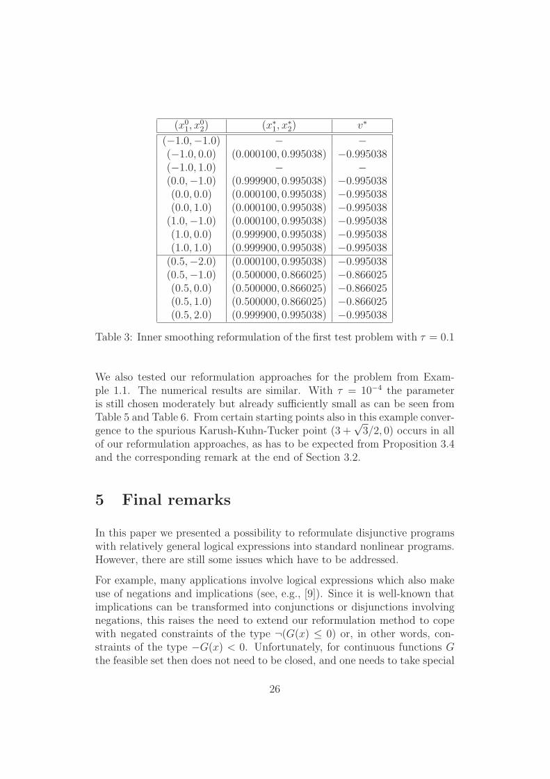
(x01, x02) (x∗1, x

∗2) v∗

(−1.0,−1.0) − −(−1.0, 0.0) (0.000100, 0.995038) −0.995038(−1.0, 1.0) − −(0.0,−1.0) (0.999900, 0.995038) −0.995038(0.0, 0.0) (0.000100, 0.995038) −0.995038(0.0, 1.0) (0.000100, 0.995038) −0.995038(1.0,−1.0) (0.000100, 0.995038) −0.995038(1.0, 0.0) (0.999900, 0.995038) −0.995038(1.0, 1.0) (0.999900, 0.995038) −0.995038(0.5,−2.0) (0.000100, 0.995038) −0.995038(0.5,−1.0) (0.500000, 0.866025) −0.866025(0.5, 0.0) (0.500000, 0.866025) −0.866025(0.5, 1.0) (0.500000, 0.866025) −0.866025(0.5, 2.0) (0.999900, 0.995038) −0.995038

Table 3: Inner smoothing reformulation of the first test problem with τ = 0.1

We also tested our reformulation approaches for the problem from Exam-ple 1.1. The numerical results are similar. With τ = 10−4 the parameteris still chosen moderately but already sufficiently small as can be seen fromTable 5 and Table 6. From certain starting points also in this example conver-gence to the spurious Karush-Kuhn-Tucker point (3 +

√3/2, 0) occurs in all

of our reformulation approaches, as has to be expected from Proposition 3.4and the corresponding remark at the end of Section 3.2.

5 Final remarks

In this paper we presented a possibility to reformulate disjunctive programswith relatively general logical expressions into standard nonlinear programs.However, there are still some issues which have to be addressed.

For example, many applications involve logical expressions which also makeuse of negations and implications (see, e.g., [9]). Since it is well-known thatimplications can be transformed into conjunctions or disjunctions involvingnegations, this raises the need to extend our reformulation method to copewith negated constraints of the type ¬(G(x) ≤ 0) or, in other words, con-straints of the type −G(x) < 0. Unfortunately, for continuous functions Gthe feasible set then does not need to be closed, and one needs to take special

26

(x01, x02) (x∗1, x

∗2) v∗

(−1.0,−1.0) (0.000000,−0.088129) 0.000000(−1.0, 0.0) (0.000000, 0.000000) 0.000000(−1.0, 1.0) (0.000000, 0.088129) 0.000000(0.0,−1.0) (0.000000, 0.001944) 0.000000(0.0, 0.0) (0.000000, 0.000000) 0.000000(0.0, 1.0) (0.000000,−0.001944) 0.000000(1.0,−1.0) (0.000000,−0.038948) 0.000000(1.0, 0.0) (0.000000, 0.000000) 0.000000(1.0, 1.0) (0.000000, 0.038948) 0.000000(2.0,−1.0) (4.000000, 0.500000) −4.000000(2.0, 0.0) (3.866026, 0.000001) −3.866026(2.0, 1.0) (4.000000,−0.500000) −4.000000(3.0,−1.0) (4.000000, 0.500000) −4.000000(3.0, 0.0) (4.000000, 0.500000) −4.000000(3.0, 1.0) (4.000000,−0.500000) −4.000000(4.0,−1.0) (0.000000,−0.041141) 0.000000(4.0, 0.0) (0.000000, 0.000000) 0.000000(4.0, 1.0) (0.000000, 0.041143) 0.000000

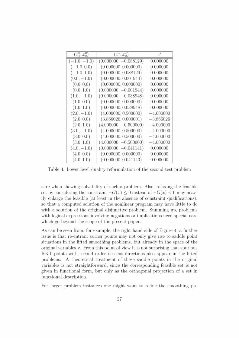
Table 4: Lower level duality reformulation of the second test problem

care when showing solvability of such a problem. Also, relaxing the feasibleset by considering the constraint −G(x) ≤ 0 instead of −G(x) < 0 may heav-ily enlarge the feasible (at least in the absence of constraint qualifications),so that a computed solution of the nonlinear program may have little to dowith a solution of the original disjunctive problem. Summing up, problemswith logical expressions involving negations or implications need special carewhich go beyond the scope of the present paper.

As can be seen from, for example, the right hand side of Figure 4, a furtherissue is that re-entrant corner points may not only give rise to saddle pointsituations in the lifted smoothing problems, but already in the space of theoriginal variables x. From this point of view it is not surprising that spuriousKKT points with second order descent directions also appear in the liftedproblems. A theoretical treatment of these saddle points in the originalvariables is not straightforward, since the corresponding feasible set is notgiven in functional form, but only as the orthogonal projection of a set infunctional description.

For larger problem instances one might want to refine the smoothing pa-

27

(x01, x02) (x∗1, x

∗2) v∗

(−1.0,−1.0) (0.000000,−0.240750) 0.000000(−1.0, 0.0) (0.000000, 0.000000) 0.000000(−1.0, 1.0) (0.000000, 0.240750) 0.000000(0.0,−1.0) (0.000000, 0.195208) 0.000000(0.0, 0.0) (0.000000, 0.000000) 0.000000(0.0, 1.0) (0.000000,−0.195208) 0.000000(1.0,−1.0) (0.000000, 0.020345) 0.000000(1.0, 0.0) (0.000000, 0.000000) 0.000000(1.0, 1.0) (0.000000,−0.020345) 0.000000(2.0,−1.0) (4.000000,−0.500000) −4.000000(2.0, 0.0) (0.000000, 0.000000) 0.000000(2.0, 1.0) (4.000000, 0.500000) −4.000000(3.0,−1.0) (4.000000,−0.500000) −4.000000(3.0, 0.0) (3.866025, 0.000000) −3.866025(3.0, 1.0) (4.000000, 0.500000) −4.000000(4.0,−1.0) (4.000000,−0.499999) −4.000000(4.0, 0.0) (3.866025, 0.000000) −3.866025(4.0, 1.0) (4.000000, 0.499999) −4.000000

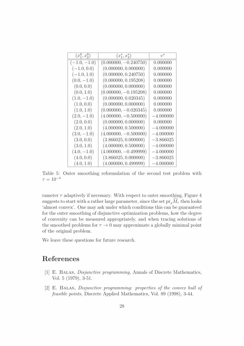
Table 5: Outer smoothing reformulation of the second test problem withτ = 10−4

rameter τ adaptively if necessary. With respect to outer smoothing, Figure 4suggests to start with a rather large parameter, since the set prxMτ then looks‘almost convex’. One may ask under which conditions this can be guaranteedfor the outer smoothing of disjunctive optimization problems, how the degreeof convexity can be measured appropriately, and when tracing solutions ofthe smoothed problems for τ → 0 may approximate a globally minimal pointof the original problem.

We leave these questions for future research.

References

[1] E. Balas, Disjunctive programming, Annals of Discrete Mathematics,Vol. 5 (1979), 3-51.

[2] E. Balas, Disjunctive programming: properties of the convex hull offeasible points, Discrete Applied Mathematics, Vol. 89 (1998), 3-44.

28

(x01, x02) (x∗1, x

∗2) v∗

(−1.0,−1.0) (0.000000,−0.240750) 0.000000(−1.0, 0.0) (0.000000, 0.000000) 0.000000(−1.0, 1.0) (0.000000, 0.240750) 0.000000(0.0,−1.0) (0.000000, 0.195205) 0.000000(0.0, 0.0) (0.000000, 0.000000) 0.000000(0.0, 1.0) (0.000000,−0.195205) 0.000000(1.0,−1.0) (0.000000, 0.020345) 0.000000(1.0, 0.0) (0.000000, 0.000000) 0.000000(1.0, 1.0) (0.000000,−0.020345) 0.000000(2.0,−1.0) (4.000000,−0.500000) −4.000000(2.0, 0.0) (0.000000, 0.000000) 0.000000(2.0, 1.0) (4.000000, 0.499999) −4.000000(3.0,−1.0) (4.000000,−0.500000) −4.000000(3.0, 0.0) (3.866025, 0.000000) −3.866025(3.0, 1.0) (4.000000, 0.500000) −4.000000(4.0,−1.0) (4.000000, 0.500000) −4.000000(4.0, 0.0) (3.866025, 0.000000) −3.866025(4.0, 1.0) (4.000000,−0.500000) −4.000000

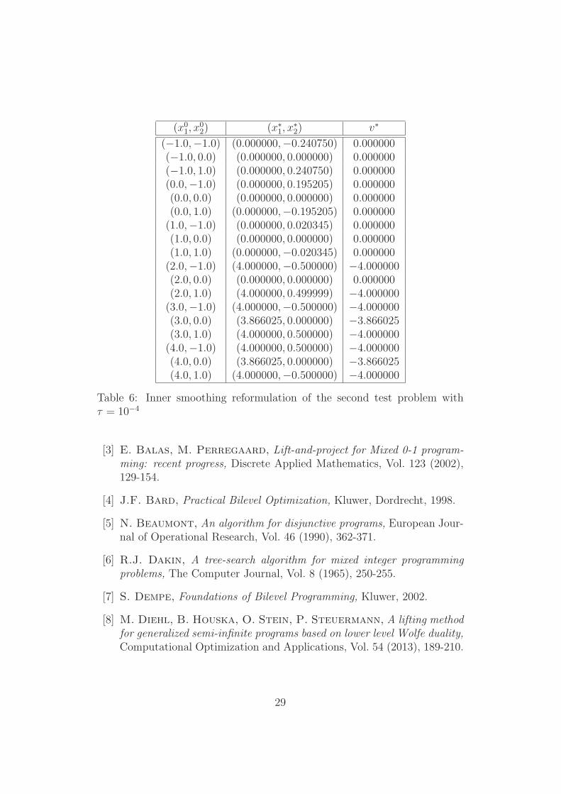
Table 6: Inner smoothing reformulation of the second test problem withτ = 10−4

[3] E. Balas, M. Perregaard, Lift-and-project for Mixed 0-1 program-ming: recent progress, Discrete Applied Mathematics, Vol. 123 (2002),129-154.

[4] J.F. Bard, Practical Bilevel Optimization, Kluwer, Dordrecht, 1998.

[5] N. Beaumont, An algorithm for disjunctive programs, European Jour-nal of Operational Research, Vol. 46 (1990), 362-371.

[6] R.J. Dakin, A tree-search algorithm for mixed integer programmingproblems, The Computer Journal, Vol. 8 (1965), 250-255.

[7] S. Dempe, Foundations of Bilevel Programming, Kluwer, 2002.

[8] M. Diehl, B. Houska, O. Stein, P. Steuermann, A lifting methodfor generalized semi-infinite programs based on lower level Wolfe duality,Computational Optimization and Applications, Vol. 54 (2013), 189-210.

29

[9] M.A. Duran, I.E. Grossmann, An outer-approximation algorithmfor a class of mixed-integer nonlinear programs, Mathematical Program-ming, Vol. 36 (1986), 307-339.

[10] F. Facchinei, H. Jiang, L. Qi, A smoothing method for mathemati-cal programs with equilibrium constraints, Mathematical Programming,Vol. 85 (1999), 107-134.

[11] R. Fletcher, S. Leyffer, Solving mixed integer nonlinear programsby outer approximation, Mathematical Programming, Vol. 66 (1994),327-349.

[12] M.A. Goberna, M.A. Lopez, Linear Semi-infinite Optimization,Wi-ley, Chichester, 1998.

[13] I.E. Grossmann, Review of nonlinear mixed-integer and disjunctiveprogramming techniques, Optimization and Engineering, Vol. 3 (2002),227-252.

[14] I.E. Grossmann, S. Lee, Generalized convex disjunctive program-ming: nonlinear convex hull relaxation, Computational Optimizationand Applications, Vol. 26 (2003), 83-100.

[15] F. Guerra Vazquez, J.-J. Ruckmann, O. Stein, G. Still, Gen-eralized semi-infinite programming: a tutorial, Journal of Computa-tional and Applied Mathematics, Vol. 217 (2008), 394-419.

[16] R. Hettich, K.O. Kortanek, Semi-infinite programming: theory,methods, and applications, SIAM Review, Vol. 35 (1993), 380-429.

[17] R. Hettich, P. Zencke, Numerische Methoden der Approximationund semi-infiniten Optimierung, Teubner, Stuttgart, 1982.

[18] J.N. Hooker, M.A. Osorio, Mixed logical-linear programming, Dis-crete Applied Mathematics, Vol. 96-97 (1999), 395-442.

[19] H.Th. Jongen, J.-J. Ruckmann, O. Stein, Disjunctive optimiza-tion: critical point theory, Journal of Optimization Theory and Appli-cations, Vol. 93 (1997), 321-336.

[20] S. Lee, I.E. Grossmann, New algorithms for nonlinear generalizeddisjunctive programming, Computers and Chemical Engineering, Vol. 24(2000), 2125-2141.

30

[21] S. Lee, I.E. Grossmann, A global optimization algorithm for non-convex generalized disjunctive programming and applications to processsystems, Computers and Chemical Engineering, Vol. 25 (2001), 1675-1697.

[22] E. Levitin, R. Tichatschke, A branch-and-bound approach for solv-ing a class of generalized semi-infinite programming problems, Journalof Global Optimization, Vol. 13 (1998), 299-315.

[23] M. Lopez, G. Still, Semi-infinite Programming, European Journalof Operational Research, Vol. 180 (2007), 491-518.

[24] G.L. Nemhauser, L.A. Wolsey, Integer and Combinatorial Opti-mization, John Wiley & Sons, New York, 1988.

[25] E. Polak, Optimization. Algorithms and Consistent Approximations,Springer, Berlin, 1997.

[26] R. Raman, I.E. Grossmann, Relations between MILP modelling andlogical inference for chemical process synthesis, Computers and Chemi-cal Engineering, Vol. 15 (1991), 73-84.

[27] R. Raman, I.E. Grossmann, Symbolic integration of logic in mixed-integer linear programming techniques for process synthesis, Computersand Chemical Engineering, Vol. 17 (1993), 909-927.

[28] R. Reemtsen, S. Gorner, Numerical methods for semi-infinite pro-gramming: a survey, in [29], 195-275.

[29] R. Reemtsen, J.-J. Ruckmann (eds), Semi-Infinite Programming,Kluwer, Boston, 1998.

[30] H. Scheel, S. Scholtes, Mathematical programs with complementar-ity constraints: Stationarity, optimality, and sensitivity, Mathematicsof Operations Research, Vol. 25 (2000), 1-22.

[31] O. Stein, Bi-level Strategies in Semi-infinite Programming, Kluwer,Boston, 2003.

[32] O. Stein, How to solve a semi-infinite optimization problem, EuropeanJournal of Operational Research, Vol. 223 (2012), 312-320.

[33] O. Stein, G. Still, On generalized semi-infinite optimization andbilevel optimization, European Journal of Operational Research, Vol. 142(2002), 444-462.

31

[34] O. Stein, G. Still, Solving semi-infinite optimization problems withinterior point techniques, SIAM Journal on Control and Optimization,Vol. 42 (2003), 769-788.

[35] O. Stein, A. Winterfeld, A feasible method for generalized semi-infinite programming, Journal of Optimization Theory and Applications,Vol. 146 (2010), 419-443.

[36] A. Wachter, L.T. Biegler, On the implementation of an interior-point filter line-search algorithm for large-scale nonlinear programming,Mathematical Programming, Vol. 106 (2006), 25-57.

[37] T. Westerlund, F. Pettersson, An extended cutting plane methodfor solving convex MINLP problems, Computers and Chemical Engi-neering, Vol. 19 (1995), 131-136.

[38] H.P. Williams, Model Building in Mathematical Programming, JohnWiley & Sons, Chichester, 1978.

32